FastDiagP: An Algorithm for Parallelized Direct Diagnosis

Abstract

Constraint-based applications attempt to identify a solution that meets all defined user requirements. If the requirements are inconsistent with the underlying constraint set, algorithms that compute diagnoses for inconsistent constraints should be implemented to help users resolve the “no solution could be found” dilemma. FastDiag is a typical direct diagnosis algorithm that supports diagnosis calculation without predetermining conflicts. However, this approach faces runtime performance issues, especially when analyzing complex and large-scale knowledge bases. In this paper, we propose a novel algorithm, so-called FastDiagP, which is based on the idea of speculative programming. This algorithm extends FastDiag by integrating a parallelization mechanism that anticipates and pre-calculates consistency checks requested by FastDiag. This mechanism helps to provide consistency checks with fast answers and boosts the algorithm’s runtime performance. The performance improvements of our proposed algorithm have been shown through empirical results using the Linux-2.6.3.33 configuration knowledge base.

Introduction

In many applications of constraint-based representations such as knowledge-based configuration (Stumptner 1997), recommendation (Felfernig and Burke 2008), automated analysis of feature models (Benavides, Segura, and Ruiz-Cortés 2010), and scheduling (Castillo et al. 2005), there exist some scenarios where over-constrained formulations occur in the underlying constraint sets (Felfernig et al. 2010; Jannach, Schmitz, and Shchekotykhin 2015). Some examples thereof are inconsistencies between the knowledge base and a set of test cases (Felfernig et al. 2004; Le et al. 2021), or inconsistencies between user requirements and the knowledge base (Felfernig et al. 2009). In such scenarios, diagnosis detection mechanisms are essential to identify preferred minimal sets of constraints (i.e., diagnoses) that are less important (from the user’s point of view) and can be adapted or deleted to restore consistency in the knowledge base (Reiter 1987; Felfernig, Schubert, and Zehentner 2012).

Direct diagnosis techniques have been recognized as efficient solutions in identifying faulty constraints without predetermining the corresponding conflict sets (Felfernig, Schubert, and Zehentner 2012; Felfernig et al. 2018). FastDiag (Felfernig, Schubert, and Zehentner 2012) is a typical example of these techniques, designed to find one preferred minimal diagnosis at a time within a given set of constraints ($C$). The algorithm divides $C$ into two subsets. If a subset is consistent, then diagnosis detection must not be applied to this subset since no diagnosis elements can be found in it. This way, $C$ can be reduced by half, and the algorithm returns one preferred minimal diagnosis at a time. Although FastDiag works efficiently in many scenarios, there exist cases where it faces runtime issues, especially in interactive settings, where users are interacting with a configurator with a huge and complex knowledge base and expect to receive instant responses (Felfernig et al. 2018).

Consistency checking is an expensive computational task that makes up most of FastDiag’s execution time (Felfernig et al. 2014). A practical solution for this issue is to pre-calculate in parallel consistency checks potentially required by FastDiag. This solution provides fast answers for consistency checks (via simple lookup in a list of already-calculated consistency checks instead of a direct solver call), which helps to accelerate the algorithm’s execution. Based on this idea, we propose in this paper a novel diagnosis detection algorithm, so-called FastDiagP, dealing with FastDiag’s run-time limitation. FastDiagP is a parallelized version of FastDiag, adopting the speculative programming principle (Burton 1985) to pre-calculate consistency checks. Although this principle is not new, modern CPUs with integrated parallel computation capabilities now make it possible to implement some speculative approaches.

The contributions of our paper are three-fold. First, we show how to parallelize direct diagnosis based on a flexible look-ahead strategy to scale its performance depending on the number of available computing cores. Second, we show how to integrate the proposed approach into FastDiag, which is applicable to interactive constraint-based applications. Third, using the inconsistent Linux-2.6.33.3 feature model taken from Diverso Lab’s benchmark (Heradio et al. 2022), we show the performance improvements of FastDiagP when working with large-scale configuration knowledge bases. Particularly, this algorithm improves the performance of diagnosis detection tasks scaling with available CPU cores, making it possible to efficiently solve more complex diagnosis problems.

Related Work

Solution Search. The increasing size and complexity of knowledge bases have led to the need of improving search solutions (Bordeaux, Hamadi, and Samulowitz 2009; Gent et al. 2018). Such solutions have been implemented as parallelization algorithms in different contexts. For example, (Bordeaux, Hamadi, and Samulowitz 2009) propose a parallelization approach to determine solutions for sub-problems independent of available cores. Due to the development of multi-core CPU architectures, parallelization approaches have become increasingly popular to exploit computing resources better and obtain expected results more efficiently.

Conflict Detection. Determining more efficiently minimal conflicts is a core requirement in many application settings (Jannach, Schmitz, and Shchekotykhin 2015). In constraint-based reasoning scenarios, the QuickXplan algorithm (Junker 2004) is applied to identify minimal conflict sets following the divide-and-conquer-based strategy. Although this algorithm helps to reduce the number of needed consistency checks significantly and supports interactive settings, it faces runtime performance issues. In this context, (Vidal et al. 2021) proposes a conflict detection approach based on speculative programming, called the so-called parallelized QuickXPlain. The empirical results show that this approach helps to significantly improve the runtime performance of QuickXplan.

Conflict Resolution. Conflict detection is the basis of conflict resolution that attempts to identify sets of minimal diagnoses (Reiter 1987; Marques-Silva et al. 2013). For instance, (Jannach, Schmitz, and Shchekotykhin 2015, 2016) propose approaches to parallelize the computation of hitting sets (diagnoses). In these studies, a level-wise expansion of a breadth-first search tree is adopted to parallelize model-based diagnosis (Reiter 1987) and compute minimal cardinality diagnoses. However, the determination of individual conflict sets is still a sequential process (based on QuickXPlain (Junker 2004)). In another study, (Jannach, Schmitz, and Shchekotykhin 2016) replace the level-wise expansion with a full hitting set parallelization and take into account additional mechanisms to ensure diagnosis minimality. Although the mentioned approaches focus on the parallelization of conflict resolution, they do not offer solutions to increase the efficiency of conflict detection. In this paper, based on the speculative programming principle (Burton 1985), we propose an algorithm integrating a parallelized conflict resolution mechanism that helps to significantly improve the runtime performance of direct diagnosis processes.

Example Configuration Knowledge Base

For demonstration purposes, we introduce a working example with a configuration knowledge base from the smartwatch domain. A Smartwatch must have at least one type of Connector and Screen. The connector can be one or more out of the following: GPS, Cellular, Wifi, or Bluetooth. The screen can be either Analog, High Resolution, or E-ink. A Smartwatch may include a Camera and a Compass. Besides, Compass requires GPS and Camera requires High Resolution. Finally, Cellular and Analog exclude each other.

Our simplified configuration knowledge base can be represented as a configuration task which is defined as a constraint satisfaction problem (CSP) (Rossi, van Beek, and Walsh 2006). A configuration task and its configuration (solution) are defined as follows (Hotz et al. 2014):

Definition 1 (Configuration task).

A configuration task can be defined as a CSP $(V,D,C)$ where $V=\{v_{1},v_{2}\mathrel{{.}\,{.}}\nobreak v_{n}\}$ is a set of variables, $D=\{dom(v_{1}),dom(v_{2})\mathrel{{.}\,{.}}\nobreak dom(v_{n})\}$ is a set of domains for each of the variables in $V$, and $C=C_{KB}\cup C_{R}$ is a set of constraints restricting possible solutions for a configuration task. $C_{KB}$ represents the configuration knowledge base (the configuration model) and $C_{R}$ represents a set of user requirements.

Definition 2 (Configuration).

A configuration (solution) $S$ for a given configuration task $(V,D,C)$ is an assignment $A=\{v_{1}=a_{1}\mathrel{{.}\,{.}}\nobreak v_{n}=a_{n}\}$, $a_{i}\in dom(v_{i})$. $S$ is valid if it is complete (i.e., each variable in $V$ has a value) and consistent (i.e., $S$ fulfills the constraints in $C$).

Example 1 (CSP-based representation of a Smartwatch configuration task).

A CSP-based representation of a configuration task $(V,D,C=C_{KB}\cup C_{R})$ that can be generated from our simplified configuration knowledge base is the following (see Table 1 for constraints in $C_{KB}$ and $C_{R}$):

• $V=\{Smartwatch$, $Connector$, $Screen$, $Camera$, $Compass$, $GPS$, $Cellular$, $Wifi$, $Bluetooth$, $Analog$, $High$ $Resolution$, $E$-$ink\}$,

• $D=\{dom(Smartwatch)\mathrel{{.}\,{.}}\nobreak dom(E$-$ink)\}$, where $dom(v_{i})$ $=\{(t)rue,(f)alse\}$,

• $C_{KB}=\{c_{0}\mathrel{{.}\,{.}}\nobreak c_{9}$}, $C_{R}=\{c_{10}\mathrel{{.}\,{.}}\nobreak c_{13}\}$.

According to Table 1, we can observe that some constraints in $C_{R}$ are inconsistent with the constraints in $C_{KB}$. For instance, $c_{10}$ and $c_{11}$ in $C_{R}$ are inconsistent with $c_{9}$ in $C_{KB}$. Therefore, no solution can be found for this configuration task. For related faulty constraints, see Example 2.∎

	CSP representation
	Constraints in the knowledge base - $C_{KB}$
$c_{0}$	$Smartwatch=t$
$c_{1}$	$Smartwatch\leftrightarrow Connector$
$c_{2}$	$Smartwatch\leftrightarrow Screen$
$c_{3}$	$Camera\rightarrow Smartwatch$
$c_{4}$	$Compass\rightarrow Smartwatch$
$c_{5}$	$Connector\leftrightarrow(GPS\vee Cellular\vee Wifi\vee Bluetooth)$
$c_{6}$	$Screen\leftrightarrow xor(Analog,High$ $Resolution,E$-$ink)$
$c_{7}$	$Camera\rightarrow High$ $Resolution$
$c_{8}$	$Compass\rightarrow GPS$
$c_{9}$	$\neg(Cellular\wedge Analog)$
	User requirements - $C_{R}$
$c_{10}$	$Cellular=t$	$c_{12}$	$Compass=t$
$c_{11}$	$Analog=t$	$c_{13}$	$GPS=f$

Table 1: Constraints in $C_{KB}=\{c_{0}\mathrel{{.}\,{.}}\nobreak c_{9}\}$ derived from our simplified configuration knowledge base, $C_{R}=\{c_{10}\mathrel{{.}\,{.}}\nobreak c_{13}\}$ is a set of user requirements.

Due to inconsistent constraints in the knowledge base/user requirements, the reasoning engine (e.g., constraint solver) cannot determine a solution. In this context, identifying explanations (in terms of diagnoses) is extremely important to help users adapt their requirements and thus restore consistency. In the next section, we introduce basic concepts regarding diagnoses and preferred minimal diagnoses. Also, we revisit the FastDiag algorithm (Felfernig, Schubert, and Zehentner 2012) and show how a preferred minimal diagnosis can be determined using this algorithm.

Determination of Preferred Diagnoses

Since the notions of a (minimal) conflict and a (minimal) diagnosis will be used in the following sections, we provide the corresponding definitions here. We use consistent($C$) to denote that the constraint set $C$ is consistent, and inconsistent($C$) to denote that the constraint set $C$ is inconsistent.

A conflict set can be defined as a minimal set of constraints that is responsible for an inconsistency, i.e., a situation in which no solution can be found for a given set of constraints $C$ (see Definition 3).

Definition 3 (Conflict set).

A conflict set is a set $CS\subseteq C:$ inconsistent($CS$). $CS$ is minimal iff $\nexists CS^{\prime}:CS^{\prime}\subset CS$.

Example 2 (Minimal conflict sets).

We are able to identify the following minimal conflict sets: $CS_{1}=\{c_{10},c_{11}\}$ and $CS_{2}=\{c_{12},c_{13}\}$. The minimality property is fulfilled since $\nexists CS_{3}:CS_{3}\subset CS_{1}$ and $\nexists CS_{4}:CS_{4}\subset CS_{2}$.∎

In order to resolve all conflicts, we need to determine corresponding hitting sets (also denoted as diagnoses (Reiter 1987)) that have to be adapted or deleted to make the user requirements consistent with the knowledge base. Based on the definition of a conflict set, we now introduce the definition of a diagnosis task and a corresponding diagnosis.

Definition 4 (Diagnosis task).

A diagnosis task can be defined by a tuple $(C_{R},C_{KB})$, where $C_{R}$ is a set of user requirements to be analyzed and $C_{KB}$ is a set of constraints specifying the configuration knowledge base.

Definition 5 (Diagnosis and Maximal Satisfiable Subset).

A diagnosis $\Delta$ of a diagnosis task $(C_{R},C_{KB})$ is a set $\Delta\subseteq C_{R}:$ consistent($C_{R}\setminus\Delta\cup C_{KB}$). $\Delta$ is minimal iff $\nexists\Delta^{\prime}:\Delta^{\prime}\subset\Delta$. A complement of $\Delta$ (i.e., $C_{R}\setminus\Delta$) is denoted as Maximal Satisfiable Subset (MSS) $\Omega$.

Example 3 (Minimal diagnoses).

Applying conflict-directed diagnosis approaches (Reiter 1987) to the diagnosis task $(C_{R}=\{c_{10}\mathrel{{.}\,{.}}\nobreak c_{13}\},C_{KB}=\{c_{0}\mathrel{{.}\,{.}}\nobreak c_{9}\})$ presented in Examples 1 and 2, the corresponding minimal diagnoses are the following: $\Delta_{1}=\{c_{10},c_{12}\}$, $\Delta_{2}=\{c_{10},c_{13}\}$, $\Delta_{3}=\{c_{11},c_{12}\}$, and $\Delta_{4}=\{c_{11},c_{13}\}$.∎

Preferred Diagnosis

To resolve given inconsistencies, a user has to choose a diagnosis consisting the constraints that need to be adapted/deleted. In this context, a diagnosis less important to the user is chosen first (Junker 2004). Such a diagnosis is a so-called “preferred diagnosis” (Marques-Silva and Previti 2014) (defined in Definition 8 based on Definitions 6 and 7).

Definition 6 (Strict total order).

Let $<$ be a strict total order over the constraints in $C=\{c_{1}\mathrel{{.}\,{.}}\nobreak c_{m}\}$ which is represented as $\langle c_{1}<c_{2}<\mathrel{{.}\,{.}}\nobreak<c_{m}\rangle$, i.e., $c_{i}$ is preferred over $c_{i+1}$.

Definition 7 (Anti-lexicographic preference, A-Preference).

Given a strict total order $<$ over $C$, a set $X\subseteq C$ is anti-lexicographically preferred over another set $Y\subseteq C$ (denoted $X<_{antilex}Y$) iff $\exists_{i\leq k\leq m}:c_{k}\in Y\setminus X$ and $X\cap\{c_{k+1}\mathrel{{.}\,{.}}\nobreak c_{m}\}=Y\cap\{c_{k+1}\mathrel{{.}\,{.}}\nobreak c_{m}\}$.

Definition 8 (Preferred diagnosis).

A minimal diagnosis $\Delta$ for a given diagnosis task $(C_{R},C_{KB})$ is a preferred diagnosis for $(C_{R},C_{KB})$ iff $\forall\Delta^{\prime}:\Delta^{\prime}<_{antilex}\Delta$.

Given a strict total order $<$ over a set of constraints, there exists a unique preferred diagnosis.

Example 4 (A preferred diagnosis).

Given two minimal diagnoses $\Delta_{3}=\{c_{11},c_{12}\}$, $\Delta_{4}=\{c_{11},c_{13}\}$ and the strict total order $\langle c_{11}<c_{12}<c_{13}\rangle$, we can say:

• $\Delta_{3}$ is anti-lexicographically preferred over $\Delta_{4}$ since $c_{13}\in\Delta_{4}\setminus\Delta_{3}$ with $\Delta_{4}\cap\emptyset$ = $\Delta_{3}\cap\emptyset$.

• $\Delta_{4}$ is a preferred diagnosis since it contains $c_{13}$ that is less important than $c_{12}$ presented in $\Delta_{3}$.∎

FastDiag

FastDiag (Felfernig, Schubert, and Zehentner 2012) determines a diagnosis without the need of conflict detection and a related derivation of hitting sets (Reiter 1987). Algorithms 1 and 2 below show a variant of FastDiag, where Algorithm 2 - FD determines a maximal satisfiable subset $\Omega$ instead of a minimal correction subset as in the original version presented in (Felfernig, Schubert, and Zehentner 2012).

Algorithm 1 FastDiag$(C,B):\Delta$

1:  if $C=\emptyset$ or Consistent$(B\cup C)$ then

2:     return($\emptyset$)

3:  else

4:     return($C\setminus\textsc{FD}(C,B,\emptyset)$)

5:  end if

Algorithm 1 - FastDiag includes two variables $C$ and $B$, where $C$ consists of potentially faulty constraints in $C_{R}$ and $B$ contains correct constraints in $C_{KB}$. The constraint ordering in $C$ conforms to the definition of the strict total order (see Definition 6). If inconsistent($B\cup C$), then Algorithm 2 - FD is activated to identify constraints in $C$ that are responsible for the inconsistency. FD determines an MSS $\Omega$, from which the corresponding minimal diagnosis can be derived ($\Delta=C\setminus\Omega$). In FD, if consistent($B\cup C$), then $C$ is returned since no diagnosis elements can be found and $C$ becomes part of the MSS. If there is only one constraint $c_{i}$ in $C$, then $c_{i}$ is an element of a conflict since inconsistent($B\cup C$). This element is removed from $C$ (by returning an empty set) to guarantee that $C$ is an MSS. If inconsistent($B\cup C$) and $C$ has more than one element, the Split function is called to divide $C$ into two subsets $C_{l}=\{c_{1}\mathrel{{.}\,{.}}\nobreak c_{k}\}$ and $C_{r}=\{c_{k+1}\mathrel{{.}\,{.}}\nobreak c_{n}\}$, where $k=\lfloor\frac{n}{2}\rfloor$. Finally, FastDiag returns an MSS and the corresponding minimal diagnosis $\Delta$.

Algorithm 2 $\textsc{FD}(C=\{c_{1}\mathrel{{.}\,{.}}\nobreak c_{n}\},B,\rho):\Omega$

1:  if $\rho\neq\emptyset$ and $\textsc{Consistent}(B\cup C)$ then

2:     return($C$)

3:  end if

4:  if $|C|=1$ then

5:     return($\emptyset$)

6:  end if

7:  Split$(C,C_{l},C_{r})$

8:  $\Omega_{2}\leftarrow\textsc{FD}(C_{l},B,C_{r})$

9:  $\Omega_{1}\leftarrow\textsc{FD}(C_{r},B\cup\Omega_{2},C_{l}\setminus\Omega_{2})$

10:  return($\Omega_{1}\cup\Omega_{2}$)

The parameter $\rho$ in the FD algorithm plays an important role in avoiding redundant consistency checks. Assigning $C_{r}$ to $\rho$ (see line 8) triggers a consistency check for $B\cup C_{l}$. If consistent($B\cup C_{l}$), $C_{l}$ will be returned by the FD call at line 2. The FD call at line 9 does not trigger a consistency check in line 1 since $C_{l}\setminus\Omega_{2}=\emptyset$, i.e., $B\cup C_{r}\cup\Omega_{2}$ = $B\cup C_{r}\cup C_{l}$ = $B\cup C$ has been already checked. The details of how FastDiag works are shown in Figure 1 on the basis of our working example.

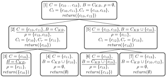
Figure 1: FD execution trace for $C=\{c_{10}\mathrel{{.}\,{.}}\nobreak c_{13}\}$ and $B=C_{KB}$. FD determines a MSS $\Omega=\{c_{10},c_{12}\}$ and the corresponding diagnosis $\Delta=\{c_{11},c_{13}\}$. The underlined $C$ and $B$ instances denote FD consistency checks.

FastDiagP - Parallelized FastDiag

General idea. FastDiagP is the parallelized version of FastDiag, in which we integrate a look-ahead mechanism adopting the speculative programming principle (Burton 1985) into the Consistent function. The look-ahead mechanism performs two tasks: (1) anticipating potential consistency checks that FastDiag might need in the near future, and (2) scheduling the asynchronous execution of anticipated consistency checks.

To ensure correct and useful anticipated consistency checks (i.e., FD will request consistency checks’ results in its next calls), the anticipation of the look-ahead mechanism complies with the two following principles P1 and P2:

- P1 (Following two assumptions concerning the consistency of $B\cup C$): In each recursive step of FD, the decision for the next recursive call depends on the consistency of the current $B\cup C$. If inconsistent($B\cup C$), FD applies the divide-and-conquer strategy to $C$. Otherwise, a strategy for $\rho$ is used, holding the sibling half of $C$. Thus, an inconsistency assumption helps to discover the next level of the FD execution tree, while a consistency one helps to exploit the sibling of the current call. This way, the look-ahead mechanism can generate all needed consistency checks without redundancy.

- P2 (Complying with the divide-and-conquer strategy of FastDiag): In each recursive step of FD, when inconsistent($B\cup C$) and $C$ is not a singleton, consistency checks for the two halves of $C$ are triggered by FD. Thus, regarding the look-ahead mechanism, when the current consideration set is not a singleton, the divide-and-conquer strategy is applied to both consistency and inconsistency assumption branches to obtain the same effect as FD can make. The current consideration set could be $C$ or $\rho$.

Besides, the anticipation considers the computer resources in terms of available CPU cores ($\#cores$) in order to generate adequate consistency checks. For instance, the current FD execution needs the consistency check for $C=\{c_{1},c_{2}\}$. The algorithm also knows that $B=\emptyset$, $\rho=\{c_{3},c_{4}\}$, i.e., the remaining constraints will be checked if $C$ is consistent, and the system has a 4-cores CPU. In this context, the look-ahead mechanism can generate and execute in parallel three consistency checks:

1. $C_{1}=\{c_{1},c_{2}\}$ - the consistency check, which is being required by FD.

2. $C_{2}=\{c_{1}\}$ - the first half of $C$, which will be checked in the next FD call if $\{c_{1},c_{2}\}$ is inconsistent.

3. $C_{3}=\{c_{1},c_{2},c_{3}\}$ - a union of $C$ and the first half of $\rho$, which will be checked if $\{c_{1},c_{2}\}$ is consistent.

Since the look-ahead mechanism runs on one CPU core, only three future consistency checks are generated in our example. Each generated consistency check is asynchronously executed in one core.

LookUp table. Consistency checks generated by the look-ahead mechanism are stored in a global LookUp table (see Table 2). If FD needs to know the consistency of a given set of constraints, a simple lookup is triggered to get the corresponding consistency check’s result. Assume that there is no consistency check for the requested set in the LookUp table. In that case, the algorithm runs the look-ahead mechanism to generate and execute in parallel anticipated consistency checks. Consistency checks in the LookUp table can also be exploited to restrict the generation of the consistency checks that have already been created in the previous steps of the look-ahead mechanism. This way, all anticipated consistency checks can be done only once and will not waste computer resources.

node-id	constraint set	consistent
$1$	$\{C_{KB}\cup\{c_{10}\mathrel{{.}\,{.}}\nobreak c_{13}\}\}$	$false$
$1.2$	$\{C_{KB}\cup\{c_{10},c_{11}\}\}$	$false$
$1.2.1$	$\{C_{KB}\cup\{c_{10},c_{11},c_{12}\}\}$	–
$1.2.1.2$	$\{C_{KB}\cup\{c_{10},c_{11},c_{13}\}\}$	–
$1.2.2$	$\{C_{KB}\cup\{c_{10}\}\}$	$true$

Table 2: A LookUp table created in our working example, including part of consistency checks generated by AddCC in the LookAhead function (see Figure 2) and executed in parallel. The ‘–’ entries indicate that the corresponding consistency checks are still ongoing or have not been started.

Consistent function. FastDiagP uses the Consistent function (see Algorithm 3) that requires three inputs: a consideration set $C$, a background knowledge $B$, and a set of constraints $\rho$ that has not been checked yet. Different from the Consistent function in FastDiag, the additional parameter $\rho$ is needed to help the look-ahead mechanism conduct inferences about future needed consistency checks. Since these sets are FD’s inputs at each recursive step, no additional computations are required.

The Consistent function checks the existence of a consistency check for $B\cup C$ in the LookUp table. If this is the case, the function returns the consistency check’s outcome. Otherwise, it activates the LookAhead function (see Algorithm 4) to generate further consistency checks that might be relevant in upcoming FD recursive calls.

Algorithm 3 Consistent$(C,B,\rho):Boolean$

1:  if $\neg\textsc{ExistCC}(B\cup C)$ then

2:     LookAhead$(C,B,\{\rho\})$

3:  end if

4:  return LookUp$(B\cup C)$

LookAhead function. The look-ahead mechanism is implemented in the recursive LookAhead function (Algorithm 4), requiring three parameters: (1) a consideration set $C$, (2) a background set $B$ holding the already-considered and assumed consistent constraints, and (3) an ordered set $\phi$ in which each item is a set of constraints to be considered when $C$ is a singleton or assumed to be consistent.

The first constraint set $\phi_{1}$ of $\phi$ is always the most recent second subset divided from $C$ in the last recursive call. $\phi_{1}$ has to be considered first when LookAhead takes into account sets of $\phi$. With the structure of $\phi$, the order of consistency checks generated by LookAhead matches the order of consistency checks requested by FastDiag. For instance, in node [1.2.2] of the LookAhead execution trace (see Figure 2), $\phi$ contains two sets: $\phi_{1}=\{c_{11}\}$ and $\phi_{2}=\{c_{12},c_{13}\}$. The set $\phi_{2}=\{c_{12},c_{13}\}$, which is added to $\phi$ in node [1], is the second half of $C=\{c_{10}\mathrel{{.}\,{.}}\nobreak c_{13}\}$. The set $\phi_{1}=\{c_{11}\}$ separated from $C=\{c_{10},c_{11}\}$ is added to $\phi$ in node [1.2]. Since $\phi_{1}$ is added later on, it will be considered first in the next LookAhead call. In particular, it is considered in node [1.2.2.2] before taking into account $\phi_{2}$ in node [1.2.2.2.1]. This mechanism works in a similar fashion as FastDiag.

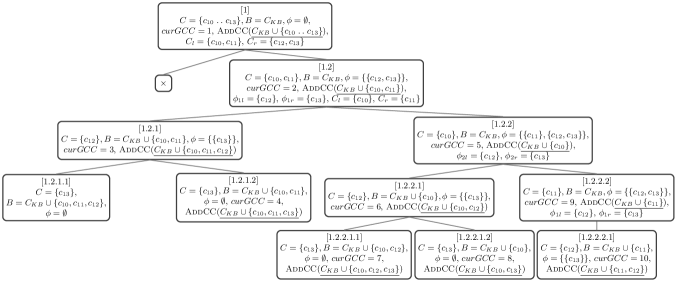
Figure 2: LookAhead execution trace for $C=\{c_{10}\mathrel{{.}\,{.}}\nobreak c_{13}\}$, $B=C_{KB}$, $\phi=\emptyset$, and $maxGCC=10$. The consistency checks $\{C_{KB}\cup\{c_{10},c_{11}\}\}$, $\{C_{KB}\cup\{c_{10}\}\}$, $\{C_{KB}\cup\{c_{10},c_{12}\}\}$, and $\{C_{KB}\cup\{c_{10},c_{12},c_{13}\}\}$ generated by LookAhead, can be used by the FastDiag execution trace illustrated in Figure 1.

Algorithm 4
LookAhead$(C,B,\phi=\{\{\phi_{1}\}\mathrel{{.}\,{.}}\nobreak\{\phi_{p}\}\})$

1:  if $curGCC<maxGCC$ then

2:     if $\neg\textsc{ExistCC}(B\cup C)$ then

3:        $curGCC\leftarrow curGCC+1$

4:        AddCC($B\cup C$)

5:     end if

6:     {$B\cup C$ assumed consistent}

7:     if $|\phi|>1\land|\phi_{1}|=1\land\textsc{ExistCC}(B\cup C\cup\phi_{1})$ then {case 1.1}

8:        Split$(\phi_{2},\phi_{2l},\phi_{2r})$

9:        LookAhead$(\phi_{2l},B\cup C,\phi_{2r}\cup(\phi\setminus\{\phi_{1},\phi_{2}\}))$

10:     else if $\phi\neq\emptyset\land|\phi_{1}|=1$ then {case 1.2}

11:        LookAhead$(\phi_{1},B\cup C,\phi\setminus\phi_{1})$

12:     else if $\phi\neq\emptyset\land|\phi_{1}|>1$ then {case 1.3}

13:        Split$(\phi_{1},\phi_{1l},\phi_{1r})$

14:        LookAhead$(\phi_{1l},B\cup C,\phi_{1r}\cup(\phi\setminus\phi_{1}))$

15:     end if

16:     {$B\cup C$ assumed inconsistent}

17:     if $|C|>1$ then {case 2.1}

18:        Split$(C,C_{l},C_{r})$

19:        LookAhead$(C_{l},B,C_{r}\cup\phi)$

20:     else if $|C|=1\land|\phi_{1}|=1$ then {case 2.2}

21:        LookAhead$(\phi_{1},B,\phi\setminus\phi_{1})$

22:     else if $|C|=1\land|\phi_{1}|>1$ then {case 2.3}

23:        Split$(\phi_{1},\phi_{1l},\phi_{1r})$

24:        LookAhead$(\phi_{1l},B,\phi_{1r}\cup(\phi\setminus\phi_{1}))$

25:     end if

26:  end if

In each LookAhead call, two global parameters $curGCC$ (initialized by zero) and $maxGCC$ (initialized by $\#cores$) are used to restrict the maximum number of generated speculative consistency checks. LookAhead checks the available space for further consistency checks and examines if any consistency check exists for $B\cup C$ so far. If not, then the $AddCC$ function is called to activate a consistency check for $B\cup C$ asynchronously and adds an entry of $B\cup C$ to the LookUp table. Next, LookAhead predicts potentially relevant consistency checks needed by FD based on two assumptions: (1) $B\cup C$ is consistent and (2) $B\cup C$ is inconsistent (see the details in the next paragraphs). The order of two assumptions is opposite to this in FastDiag since consistency checks with larger cardinality should be executed in advance, which helps reduce the waiting time in case the corresponding consistency checks are still ongoing.

Assumption 1 ($B\cup C$ is consistent): The function further checks the sets of $\phi$ when $B\cup C$ is consistent, i.e., all LookAhead calls will have $B\cup C$ as the background set.

• If there is a consistency check for $B\cup C\cup\phi_{1}$ in the LookUp table (see case 1.1 in Algorithm 4), LookAhead omits $\phi_{1}$ and further checks $\phi_{2}$. The function considers the first half of $\phi_{2}$ ($\phi_{2l}$) as the consideration set. $\{\phi_{1},\phi_{2}\}$ in $\phi$ are replaced with the second half of $\phi_{2}$ (i.e., $\phi_{2r}\cup(\phi\setminus\{\phi_{1},\phi_{2}\}$)). Let’s have a look at an example in Figure 2. In node [1.2.2], the consistency check for $C_{KB}\cup\{c_{10},c_{11}\}$ has already been generated. Hence, in node [1.2.2.1], the function omits $\phi_{1}=\{c_{11}\}$ and proceeds with a further look ahead for $\phi_{2}$.

• If $|\phi_{1}|=1$ (see case 1.2 in Algorithm 4), the input parameters of the function are $\phi_{1}$, $B\cup C$, and $\phi\setminus\phi_{1}$. In our example (Figure 2), this case will be applied to expand the consistent branch of node [1.2.2.1].

• If $|\phi_{1}|>1$ (see case 1.3 in Algorithm 4), $\phi_{1}$ is divided into two halves $\phi_{1l}$ and $\phi_{1r}$. LookAhead is called where $C$ is replaced with the first half $\phi_{1l}$ and $\phi_{1}$ in $\phi$ is replaced with the second half $\phi_{1r}$ (i.e., $\phi_{1r}\cup(\phi\setminus\phi_{1})$). One example is shown in node [1.2] of Figure 2.

Assumption 2 ($B\cup C$ is inconsistent): Consistency checks for the halves of $C$ are necessary to identify elements of $C$ responsible for the inconsistency.

• If the cardinality of $C$ is greater than 1 (see case 2.1 in Algorithm 4), $C$ is divided into two halves $C_{l}$ and $C_{r}$. Thereafter, LookAhead for $C_{l}$ is called, where $B\cup C_{l}$ becomes the next consistency check, and $C_{r}$ is stored in $\phi$ to be considered when $B\cup C_{l}$ is assumed to be consistent or $C_{l}$ is a singleton. Note that $C_{r}$ is added to the head of $\phi$ to be considered first when the function takes into account the sets of $\phi$. Examples of this case are shown in nodes [1] and [1.2] of Figure 2.

• If $|C|=1$, the function further checks the sets of $\phi$ with the inconsistency assumption:

  • If the first set of $\phi$ is a singleton ($|\phi_{1}|=1$) (see case 2.2 in Algorithm 4), LookAhead is called, where $C$ is replaced with $\phi_{1}$ and $\phi_{1}$ is removed from $\phi$. The execution of LookAhead according to this case can be found in nodes [1.2.1] and [1.2.2] of Figure 2.

  • If $\phi_{1}$ consists of several constraints to be considered ($|\phi_{1}|>1$) (see case 2.3 in Algorithm 4), $\phi_{1}$ is divided into two halves $\phi_{1l}$ and $\phi_{1r}$. The function LookAhead is called, where the first half $\phi_{1l}$ is the consideration set, $\phi_{1}$ in $\phi$ is replaced with $\phi_{1r}$ (i.e., $\phi_{1r}\cup(\phi\setminus\phi_{1})$). In Figure 2, the inconsistent branch of node [1.2.2.2] is created based on this case.

Theoretical Analysis of FastDiagP

Soundness and Completeness of FastDiagP. FastDiagP preserves the soundness and completeness properties of FastDiag. FastDiagP does not change the FD function but integrates the look-ahead mechanism, where some consistency checks requested by FD are pre-calculated. Besides, FD performs simple lookups instead of expensive solver calls. Therefore, FastDiagP obtains better performance, and the returned diagnosis is minimal and preferred.

Soundness and Completeness of LookAhead. LookAhead generates correct consistency checks for subsets of the consideration set $C$. Assuming that $C^{\prime}$ is a set generated by LookAhead, but $C^{\prime}\not\subseteq(C\cup\phi)$. We can say that $\exists c_{k}:c_{k}\in C^{\prime}\land c_{k}\not\in(C\cup\phi)$. Since LookAhead does not exploit constraints outside of $C\cup\phi$, $C^{\prime}$ is not a set generated by LookAhead. Besides, by following two principles P1 and P2, LookAhead can generate all possible combinations of constraints in $C$.

Uniqueness of anticipated consistency checks. LookAhead exploits $\phi$ in both assumption branches, which leads to redundant consistency checks when exploiting $\phi$ according to the consistency assumption. The checks in lines 2 and 7 (Algorithm 4) assure that generated consistency checks are unique.

Complexity analysis. FD complexity. The worst-case complexity of FD in terms of the number of needed consistency checks for determining MSS $\Omega$ and the corresponding diagnosis $\Delta=C-\Omega$ is $2d\times log_{2}(\frac{n}{d})+2d$, where $d$ is the set size of the minimal diagnosis, $n$ is the number of constraints in $C$, and $2d$ represents the branching factor and the number of leaf-node consistency checks. The best-case complexity is $log_{2}(\frac{n}{d})+2d$. In the worst case, each diagnosis element is located in a different path of the search tree. The factor $log_{2}(\frac{n}{d})$ represents the depth of a path of the FD search tree. In the best case, all constraints part of a diagnosis are included in a single path of the search tree.

LookAhead complexity. Assuming that $\phi=\emptyset$, the number of consistency checks ($N$) generated by LookAhead is the sum of all possible combinations of $n$ constraints in the consideration set $C$. It means that $N=\sum_{i=1}^{n}{{n}\choose{i}}=2^{n}-1$. Due to the uniqueness of LookAhead, the upper bound of its space complexity in terms of the number of LookAhead calls is $2^{n}-1$.

Termination of LookAhead. If $maxGCC\leq 2^{n}-1$, recursive calls of LookAhead stop when $maxGCC$ consistency checks are generated. Otherwise, LookAhead terminates if $C$ and $\phi$ are empty.

Empirical Evaluation

Experiment design. In this study, we compared the performance of FastDiagP and FastDiag according to three aspects: (1) run-time $R$ needed to determine the preferred diagnosis, (2) speedup $S$ that tells us the gain we get through the parallelization, and (3) efficiency $E$ representing the ratio between the speedup and the number of processes in which we run the algorithm. In particular, speedup $S_{p}$ is computed as $=T_{1}/T_{p}$, where $T_{1}$ is the wall time when using 1 core (FastDiag) and $T_{p}$ is the wall time when $p$ cores are used. The efficiency $E_{p}$ is defined as $S_{p}/p$. These aspects were analyzed in two dimensions: the diagnosis cardinality and the available computing cores ($\#cores$).

Dataset and Procedure. The basis for these evaluations was the Linux-2.6.33.3 configuration knowledge base taken from Diverso Lab’s benchmark (Heradio et al. 2022). The characteristics of this knowledge base are the following: $\#$features = 6,467; $\#$relationships = 6,322; and $\#$cross-tree constraints = 7,650. For this knowledge base, we randomly synthesized and collected 20,976 inconsistent sets of requirements, whose cardinality ranges from 5 to 250. We applied systematic sampling technique (Mostafa and Ahmad 2018) to select 10 inconsistent requirements with diagnosis cardinalities of 1, 2, 4, 8, and 16.

The diagnosis algorithms were implemented in Python using Sat4j (Le Berre and Parrain 2010) as a reasoning solver. We used the CNF class of PySAT (Ignatiev, Morgado, and Marques-Silva 2018) for representing constraints and the Python multiprocessing package for running parallel tasks. All experiments reported in the paper were conducted with an Amazon EC2 instance of the type c5a.8xlarge, offering 32 vCPUs with 64-GB RAM.

			$\#cores$
			1	4	8	16	32
$|diag|$	1	$R$	4.56	3.08	2.77	2.63	3.29
		$S$		1.48	1.65	1.74	1.39
		$E$		0.49	0.24	0.12	0.05
	2	$R$	5.60	4.00	3.69	3.71	5.05
		$S$		1.40	1.52	1.51	1.11
		$E$		0.47	0.22	0.10	0.04
	4	$R$	8.13	5.95	5.76	6.43	10.11
		$S$		1.37	1.41	1.26	0.80
		$E$		0.46	0.20	0.08	0.03
	8	$R$	11.96	9.06	8.74	9.63	14.52
		$S$		1.32	1.37	1.24	0.82
		$E$		0.44	0.20	0.08	0.03
	16	$R$	20.95	16.80	16.38	19.02	29.28
		$S$		1.25	1.28	1.10	0.72
		$E$		0.42	0.18	0.07	0.02

Table 3: Average runtime $R$ (in $sec$), speedup $S$, and efficiency $E$ of FastDiagP ($\#cores>1$) versus FastDiag ($\#cores=1$) needed for determining the preferred diagnosis with a repetition rate of 3 per setting and $maxGCC=\#cores-1$. $|diag|$ denotes the cardinality of the diagnosis.

		$\#cores$
		1	8	16	32
$|diag|$	1	4.56	2.78	2.79	2.81
	2	5.60	3.69	3.70	3.72
	4	8.13	5.76	5.80	5.87
	8	11.96	8.74	8.78	8.84
	16	20.95	16.38	16.41	16.64

Table 4: Average runtime (in $sec$) of FastDiagP ($\#cores>1$) versus FastDiag ($\#cores=1$) needed for determining the preferred diagnosis with a repetition rate of 3 per setting and $maxGCC=7$. $|diag|$ denotes the cardinality of the preferred diagnosis. The bold values prove the optimal number of CPU cores ($\#cores=8$).

Results. The experimental results show that FastDiagP outperforms the sequential direct diagnosis approach in almost all scenarios (see the bold values in Table 3). Besides, in Tables 3 and 4, the optimal number of CPU cores is 8 and the corresponding speedup values range from 1.28 to 1.65, showing the runtime deduction up to 40%. The $\#cores$ higher than 8 becomes less efficient for boosting the performance. Particularly, in Table 3, the increase of $\#cores$ (that also triggers the increase of $maxGCC$ ($maxGCC=\#cores-1$)) leads to gradual runtime increase (i.e., lower performance). A parallelization mechanism with more than 8 cores is not so much helpful in such a scenario. This manifests when $\#cores=32$, $maxGCC=31$, and $|diag|=4,8,16$. The reason is that the LookAhead function applies a sequential mechanism. When $maxGCC$ gets higher, the runtime of LookAhead increases exponentially, leading to a significant increase of FastDiagP’s runtime. Besides, Table 4 confirms that the utilization of more than 8 CPU cores becomes less efficient. In this evaluation, our idea was to fix the $maxGCC$ value ($maxGCC=7$) to see how the performance of FastDiagP is when $\#cores$ is higher than 8.

Conclusion

In this paper, we have proposed a parallelized variant of the FastDiag algorithm to diagnose over-constrained problems. Our parallelized approach helps to exploit multi-core architectures and provides an efficient preferred diagnosis detection mechanism. Furthermore, our approach is helpful for dealing with complex over-constrained problems, boosting the performance of various knowledge-based applications, and making these systems more accessible, especially in the context of interactive settings. Open topics for future research are the following: (1) performing more in-depth evaluations on the basis of industrial configuration knowledge bases (in this context, we plan to analyze the different look-ahead search approaches, e.g. breadth-first search, in further detail), and (2) applying speculative reasoning for supporting anytime diagnosis tasks.

References

- Benavides, Segura, and Ruiz-Cortés (2010) Benavides, D.; Segura, S.; and Ruiz-Cortés, A. 2010. Automated Analysis of Feature Models 20 Years Later: A Literature Review. Information Systems, 35(6): 615–636.
- Bordeaux, Hamadi, and Samulowitz (2009) Bordeaux, L.; Hamadi, Y.; and Samulowitz, H. 2009. Experiments with Massively Parallel Constraint Solving. In 21st International Joint Conference on Artifical Intelligence, 443–448. California, USA: Morgan Kaufmann.
- Burton (1985) Burton, F. W. 1985. Speculative computation, parallelism, and functional programming. IEEE Transactions on Computers, C-34(12): 1190–1193.
- Castillo et al. (2005) Castillo, L.; Borrajo, D.; Salido, M.; and Oddi, A. 2005. Planning, Scheduling and Constraint Satisfaction: From Theory to Practice, volume 117 of Frontiers in Artificial Intelligence and Applications. IOPress.
- Felfernig and Burke (2008) Felfernig, A.; and Burke, R. 2008. Constraint-based Recommender Systems: Technologies and Research Issues. In ACM International Conference on Electronic Commerce (ICEC’08), 17–26. Innsbruck, Austria.
- Felfernig et al. (2004) Felfernig, A.; Friedrich, G.; Jannach, D.; and Stumptner, M. 2004. Consistency-based diagnosis of configuration knowledge bases. Artificial Intelligence, 152: 213–234.
- Felfernig et al. (2009) Felfernig, A.; Friedrich, G.; Schubert, M.; Mandl, M.; Mairitsch, M.; and Teppan, E. 2009. Plausible Repairs for Inconsistent Requirements. In Proceedings of the 21st International Jont Conference on Artifical Intelligence (IJCAI’09), 791–796. California, USA: Morgan Kaufmann.
- Felfernig et al. (2014) Felfernig, A.; Hotz, L.; Bagley, C.; and Tiihonen, J. 2014. Knowledge-based Configuration: From Research to Business Cases. San Francisco, CA, USA: Morgan Kaufmann Publishers Inc., 1 edition. ISBN 012415817X, 9780124158177.
- Felfernig et al. (2010) Felfernig, A.; Schubert, M.; Mandl, M.; Friedrich, G.; and Teppan, E. 2010. Efficient Explanations for Inconsistent Constraint Sets. In ECAI 2010 - 19th European Conference on Artificial Intelligence, Lisbon, Portugal, August 16-20, 2010, 1043–1044. IOS Press.
- Felfernig, Schubert, and Zehentner (2012) Felfernig, A.; Schubert, M.; and Zehentner, C. 2012. An Efficient Diagnosis Algorithm for Inconsistent Constraint Sets. Artif. Intell. Eng. Des. Anal. Manuf., 26(1): 53–62.
- Felfernig et al. (2018) Felfernig, A.; Walter, R.; Galindo, J. A.; Benavides, D.; Erdeniz, S. P.; Atas, M.; and Reiterer, S. 2018. Anytime diagnosis for reconfiguration. J. Intell. Inf. Syst., 51(1): 161–182.
- Gent et al. (2018) Gent, I.; Miguel, I.; Nightingale, P.; McCreesh, C.; Prosser, P.; Nooore, N.; and Unsworth, C. 2018. A Review of Literature on Parallel Constraint Solving. Theory and Practice of Logic Programming, 18(5–6): 725–758.
- Heradio et al. (2022) Heradio, R.; Fernandez-Amoros, D.; Galindo, J. A.; Benavides, D.; and Batory, D. 2022. Uniform and scalable sampling of highly configurable systems. Empirical Software Engineering, 27(2): 44.
- Hotz et al. (2014) Hotz, L.; Felfernig, A.; Stumptner, M.; Ryabokon, A.; Bagley, C.; and Wolter, K. 2014. Configuration Knowledge Representation and Reasoning. In Felfernig, A.; Hotz, L.; Bagley, C.; and Tiihonen, J., eds., Knowledge-based Configuration – From Research to Business Cases, 41 – 72. Boston: Morgan Kaufmann.
- Ignatiev, Morgado, and Marques-Silva (2018) Ignatiev, A.; Morgado, A.; and Marques-Silva, J. 2018. PySAT: A Python Toolkit for Prototyping with SAT Oracles. In SAT, 428–437.
- Jannach, Schmitz, and Shchekotykhin (2015) Jannach, D.; Schmitz, T.; and Shchekotykhin, K. 2015. Parallelized Hitting Set Computation for Model-Based Diagnosis. In 29th AAAI Conference on Artificial Intelligence, 1503–1510. Austin, Texas: AAAI Press.
- Jannach, Schmitz, and Shchekotykhin (2016) Jannach, D.; Schmitz, T.; and Shchekotykhin, K. 2016. Parallel Model-Based Diagnosis on Multi-Core Computers. Journal of Artificial Intelligence Research, 55: 835–887.
- Junker (2004) Junker, U. 2004. QuickXPlain: Preferred Explanations and Relaxations for over-Constrained Problems. In Proceedings of the 19th National Conference on Artifical Intelligence, AAAI’04, 167–172. AAAI Press.
- Le et al. (2021) Le, V.-M.; Felfernig, A.; Uta, M.; Benavides, D.; Galindo, J.; and Tran, T. N. T. 2021. DirectDebug: Automated Testing and Debugging of Feature Models. In 2021 IEEE/ACM 43rd International Conference on Software Engineering: New Ideas and Emerging Results (ICSE-NIER), 81–85.
- Le Berre and Parrain (2010) Le Berre, D.; and Parrain, A. 2010. The Sat4j library, release 2.2. Journal on Satisfiability, Boolean Modeling and Computation, 7(2-3): 59–64.
- Marques-Silva et al. (2013) Marques-Silva, J.; Heras, F.; Janota, M.; Previti, A.; and Belov, A. 2013. On Computing Minimal Correction Subsets. In 23rd International Joint Conference on Artificial Intelligence, 615–622. Beijing, China.
- Marques-Silva and Previti (2014) Marques-Silva, J.; and Previti, A. 2014. On Computing Preferred MUSes and MCSes. In Theory and Applications of Satisfiability Testing – SAT 2014, 58–74. Cham: Springer.
- Mostafa and Ahmad (2018) Mostafa, S. A.; and Ahmad, I. A. 2018. Recent developments in systematic sampling: A review. Journal of Statistical Theory and Practice, 12(2): 290–310.
- Reiter (1987) Reiter, R. 1987. A Theory of Diagnosis from First Principles. Artif. Intell., 32(1): 57–95.
- Rossi, van Beek, and Walsh (2006) Rossi, F.; van Beek, P.; and Walsh, T. 2006. Handbook of Constraint Programming. Elsevier.
- Stumptner (1997) Stumptner, M. 1997. An Overview of Knowledge‐based Configuration. Ai Communications, 10(2): 111–125.
- Vidal et al. (2021) Vidal, C.; Felfernig, A.; Galindo, J.; Atas, M.; and Benavides, D. 2021. Explanations for over-constrained problems using QuickXPlain with speculative executions. Journal of Intelligent Information Systems, 57(3): 491–508.