An Information-Spectrum Approach to Distributed Hypothesis Testing for General Sources

Abstract

This paper investigates Distributed Hypothesis testing (DHT), in which a source $\mathbf{X}$ is encoded given that side information $\mathbf{Y}$ is available at the decoder only. Based on the received coded data, the receiver aims to decide on the two hypotheses $H_{0}$ or $H_{1}$ related to the joint distribution of $\mathbf{X}$ and $\mathbf{Y}$. While most existing contributions in the literature on DHT consider i.i.d. assumptions, this paper assumes more generic, non-i.i.d., non-stationary, and non-ergodic sources models. It relies on information-spectrum tools to provide general formulas on the achievable Type-II error exponent under a constraint on the Type-I error. The achievability proof is based on a quantize-and-binning scheme. It is shown that with the quantize-and-binning approach, the error exponent boils down to a trade-off between a binning error and a decision error, as already observed for the i.i.d. sources. The last part of the paper provides error exponents for particular source models, e.g., Gaussian, stationary, and ergodic models.

I Introduction

In distributed communication networks, data is gathered from various remote nodes and then sent to a server for further processing. Often, the primary objective of the server is not to reconstruct the data, but instead to make a decision based on the collected data. This type of setup is known as distributed hypothesis testing (DHT), and it was first investigated from an information-theoretic perspective in [1, 2].

In DHT, a source $\mathbf{X}$ is encoded using side information $\mathbf{Y}$ available only to the decoder, as shown in Figure 1. The receiver aims to make a decision between two hypothesis: $H_{0}$, where the joint probability distribution of $(\mathbf{X},\mathbf{Y})$ is $P_{\mathbf{X}\mathbf{Y}}$, and $H_{1}$, where the joint distribution is $P_{\overline{\mathbf{X}}\overline{\mathbf{Y}}}$. Hypothesis testing involves two types of errors, called the Type-I error and the Type-II error [3]. The information-theoretic analysis of DHT aims to determine the achievable error exponent for the Type-II error, while keeping the Type-I error below a fixed threshold [1, 2].

Previous contributions on DHT typically assume that the sources $\mathbf{X}$ and $\mathbf{Y}$ generate independent and identically distributed (i.i.d.) pairs of symbols $(X_{t},Y_{t})$ [4, 5, 6, 7, 8]. For example, [7] and [8] provide the error exponent achieved by a quantize-and-binning scheme for i.i.d. sources. Some more complex source models have been investigated in [9, 10], which assume that the sources $\mathbf{X}$ and $\mathbf{Y}$ generate pairs of Gaussian vectors $(\mathbf{X}_{t}^{M},\mathbf{Y}_{t}^{N})$ with auto-correlations embedded in each vector $\mathbf{X}_{t}^{M}$ and $\mathbf{Y}_{t}^{N}$, as well as cross-correlation between them. However, the models of [9, 10] are block-i.i.d. in the sense that the successive pairs $(\mathbf{X}_{t}^{M},\mathbf{Y}_{t}^{N})$ are assumed to be i.i.d. with $t$.

However, i.i.d. and block-i.i.d. models are often inadequate for capturing the statistics of signals like time series or videos, which cannot be decomposed into fixed-length independent blocks and are frequently non-stationary and/or non-ergodic. As a result, the objective of this paper is to consider a more general source model that is non-i.i.d. and can account for non-stationary and non-ergodic signals, while still encompassing the previous models as particular instances. To investigate DHT under these conditions, we utilize information spectrum tools, which were first introduced in [11] and generally provide information theory results that are applicable to a broad range of source models. It should be noted that information spectrum has been previously used for hypothesis testing in [12], but only for the encoding of a source $\mathbf{X}$ alone, without the use of side information $\mathbf{Y}$.

In this paper, we investigate DHT using general source models for $\mathbf{X}$ and $\mathbf{Y}$ and provide an achievability scheme that yields a general expression for the Type-II error exponent. Our approach to the achievability scheme builds upon the quantize-and-binning techniques presented in [8], while taking into account the use of side information for more complex source models. As in [8], the resulting error exponent consists of two terms: one for the binning error and the other for the decision error. We then specialize our error-exponent to specific source models of interest, including (i) i.i.d. sources, for which we recover the error exponent reported in [8]; (ii) non-i.i.d. stationary and ergodic sources in general; and (iii) non-i.i.d. Gaussian stationary and ergodic sources.

The outline of the paper is as follows. Section II describes the general sources model and restates the DHT problem. Section III provides the achievable error exponent for general sources, and Section IV derives the proof. Section V considers some examples of source models.

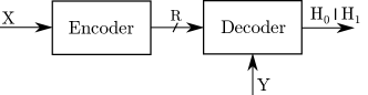
Figure 1: Distributed Hypothesis Testing coding scheme

II Problem statement

In the DHT problem shown in Fig.1, the encoder observes a source sequence $\mathbf{X}$, and the decoder receives a coded version of $\mathbf{X}$ as well as a side information sequence $\mathbf{Y}$, where $\mathbf{X}$ and $\mathbf{Y}$ are correlated. In what follows, $\llbracket 1,n\rrbracket$ denotes the set of integers between $1$ and $n$.

II-A General Sources

We consider that the sequences $\mathbf{X}$ and $\mathbf{Y}$ are produced from two general sources which are not necessarily i.i.d., and not even stationary or ergodic. As in [12], we define general sources $\mathbf{X}$ and $\mathbf{Y}$ as two infinite sequences :

$$\mathbf{X} =\left\{\mathbf{X}^{n}=\left(X_{1},X_{2},\cdots,X_{n}\right)\right\}_{n=1}^{\infty},$$

$$\mathbf{Y} =\left\{\mathbf{Y}^{n}=\left(Y_{1},Y_{2},\cdots,Y_{n}\right)\right\}_{n=1}^{\infty}$$ (1)

of $n$-dimensional random variables $\mathbf{X}^{n},\mathbf{Y}^{n}$, respectively. Each component random variable $X_{i},Y_{i}$, $i\in\llbracket 1,n\rrbracket$, takes values in a finite source alphabet $\mathcal{X},\mathcal{Y}$, respectively. In what follows, $P_{\mathbf{X}^{n}}$ is the probability distribution of the length-n vector $\mathbf{X}^{n}$, and $P_{\mathbf{X}}=\left\{P_{\mathbf{X}^{n}}\right\}_{n=1}^{\infty}$ is the collection of all probability distributions $P_{\mathbf{X}^{n}}$. The same holds for the source $\mathbf{Y}$.

We now describe two particular cases of (1). The first one consists of a scalar i.i.d. model in which the sequences $\mathbf{X}^{n}$ and $\mathbf{Y}^{n}$ come from two i.i.d. sources, i.e., the successive pairs of symbols $\left(X_{n},Y_{n}\right)$ are independent and distributed according to the same joint distribution $P_{XY}$. This model was considered for DHT in [7, 8]. The second case still relies on an i.i.d. model but for source vectors. In this case, the source sequences $\mathbf{X}^{n}$ and $\mathbf{Y}^{n}$ are defined as

$$\mathbf{X}^{n}=\left\{\mathbf{X}_{t}^{M}\right\}_{t=1}^{n},\leavevmode\nobreak\ \mathbf{Y}^{n}=\left\{\mathbf{Y}_{t}^{N}\right\}_{t=1}^{n},$$ (2)

where $\{\mathbf{X}_{t}^{M}\}_{t=1}^{n}$ and $\{\mathbf{Y}_{t}^{N}\}_{t=1}^{n}$ are sequences of i.i.d. M-dimensional and N-dimensional random vectors, respectively. This means that successive pairs of $\left(\mathbf{X}_{t}^{M},\mathbf{Y}_{t}^{N}\right)$ are independent and distributed according to the same joint distribution $P_{\mathbf{X}^{M}\mathbf{Y}^{N}}$. The i.i.d. property of the successive M-length and N-length vectors simplifies the DHT analysis by allowing for an orthogonal transform to be applied onto the successive independent blocks $\mathbf{X}_{t}^{M}$ and $\mathbf{Y}_{t}^{N}$ [9, 10]. Our model described in (1) is more general since it considers infinite sequences without the i.i.d. assumption.

II-B Distributed Hypothesis Testing

In what follows, we consider that the joint distribution of the sequence pair $\left\{\left(\mathbf{X}^{n},\mathbf{Y}^{n}\right)\right\}_{n=1}^{\infty}$ depends on the underlying hypotheses $H_{0}$ and $H_{1}$ defined as

$$H_{0}:\left(\mathbf{X}^{n},\mathbf{Y}^{n}\right)\sim P_{\mathbf{X}^{n}\mathbf{Y}^{n}},$$ (3)

$$H_{1}:\left(\mathbf{X}^{n},\mathbf{Y}^{n}\right)\sim P_{\overline{\mathbf{X}}^{n}\overline{\mathbf{Y}}^{n}}.$$ (4)

where the marginal probability distributions $P_{\mathbf{X}^{n}}$ and $P_{\mathbf{Y}^{n}}$ do not depend on the hypothesis.

We consider the following usual coding scheme defined in the literature on DHT [1, 8].

Definition 1

The encoding function $f^{(n)}$ and decoding function $g^{(n)}$ are defined as

$$f^{(n)} :\mathcal{X}^{n}\longrightarrow\mathcal{M}_{n}=\llbracket 1,M_{2}\rrbracket,$$ (5)

$$g^{(n)} :\mathcal{M}_{n}\times\mathcal{Y}^{n}\longrightarrow\mathcal{H}=\{H_{0},H_{1}\},$$ (6)

such that

$$\limsup_{n\rightarrow\infty}\frac{1}{n}\log\text{M}_{2}\leq\text{R},$$ (7)

where $R$ is the rate and $\text{M}_{2}$ is the cardinality of the alphabet set $\mathcal{M}_{n}$.

Definition 2

The Type-I and Type-II error probabilities $\alpha_{n}$ and $\beta_{n}$ are defined as

$$\alpha_{n} =\mathbb{P}\left[g^{(n)}\left(f^{(n)}\left(\mathbf{X}^{n}\right),\mathbf{Y}^{n}\right)=H_{1}\mid H_{0}\ \text{is true}\right],$$ (8)

$$\beta_{n} =\mathbb{P}\left[g^{(n)}\left(f^{(n)}\left(\mathbf{X}^{n}\right),\mathbf{Y}^{n}\right)=H_{0}\mid H_{1}\ \text{is true}\right].$$ (9)

Definition 3

The Type-II error exponent $\theta$ is said to be achievable for a given rate $R$, if for large blocklength $n$, there exists encoding and decoding functions $\left(f^{(n)},g^{(n)}\right)$ such that the Type-I and Type-II error probabilities $\alpha_{n}$ and $\beta_{n}$ satisfy

$$\alpha_{n}\leq\epsilon,$$ (10)

and

$$\limsup_{n\rightarrow\infty}\frac{1}{n}\log\frac{1}{\beta_{n}}\geq\theta$$ (11)

for any $\epsilon>0$.

In the following, we aim to determine the achievable Type-II error exponent $\theta$ for general sources.

III Main result: Error exponent

III-A Definitions

We first provide some definitions which will be useful to express our main result. The $\limsup$ and $\liminf$ in probability of a sequence $\left\{Z_{n}\right\}_{n=1}^{\infty}$ are, respectively, defined as [11]

$$\mathrm{p}-\limsup_{n\rightarrow\infty}Z_{n} =\inf\left\{\alpha\mid\lim_{n\rightarrow+\infty}\mathbb{P}\left(Z_{n}>\alpha\right)=0\right\},$$ (12)

$$\mathrm{p}-\liminf_{n\rightarrow\infty}Z_{n} =\sup\left\{\alpha\mid\lim_{n\rightarrow+\infty}\mathbb{P}\left(Z_{n}<\alpha\right)=0\right\}.$$ (13)

The spectral sup-mutual information $\overline{I}(\mathbf{X};\mathbf{U})$, the spectral inf-mutual information $\underline{I}(\mathbf{U};\mathbf{Y})$, the spectral inf-divergence rate $\underline{D}\left(P_{\mathbf{U}\mathbf{Y}}\|P_{\overline{\mathbf{U}}\overline{\mathbf{Y}}}\right)$, and the spectral sup-divergence rate $\overline{D}\left(P_{\mathbf{U}\mathbf{Y}}\|P_{\overline{\mathbf{U}}\overline{\mathbf{Y}}}\right)$ are, respectively, defined as [11]

$$\bar{I}(\mathbf{X};\mathbf{U})=\mathrm{p}-\limsup_{n\rightarrow\infty}\frac{1}{n}\log\frac{P_{\mathbf{U}^{n}\mid\mathbf{X}^{n}}\left(\mathbf{U}^{n}\mid\mathbf{X}^{n}\right)}{P_{\mathbf{U}^{n}}\left(\mathbf{U}^{n}\right)},$$ (14)

$$\underline{I}(\mathbf{U};\mathbf{Y})=\mathrm{p}-\liminf_{n\rightarrow\infty}\frac{1}{n}\log\frac{P_{\mathbf{U}^{n}\mid\mathbf{Y}^{n}}\left(\mathbf{U}^{n}\mid\mathbf{Y}^{n}\right)}{P_{\mathbf{U}^{n}}\left(\mathbf{U}^{n}\right)},$$ (15)

$$\underline{D}\left(P_{\mathbf{U}\mathbf{Y}}\|P_{\overline{\mathbf{U}}\overline{\mathbf{Y}}}\right)=\mathrm{p}-\liminf_{n\rightarrow\infty}\frac{1}{n}\log\frac{P_{\mathbf{U}^{n}\mathbf{Y}^{n}}\left(\mathbf{U}^{n},\mathbf{Y}^{n}\right)}{P_{\overline{\mathbf{U}}^{n}\overline{\mathbf{Y}}^{n}}\left(\mathbf{U}^{n},\mathbf{Y}^{n}\right)},$$ (16)

$$\overline{D}\left(P_{\mathbf{U}\mathbf{Y}}\|P_{\overline{\mathbf{U}}\overline{\mathbf{Y}}}\right)=\mathrm{p}-\limsup_{n\rightarrow\infty}\frac{1}{n}\log\frac{P_{\mathbf{U}^{n}\mathbf{Y}^{n}}\left(\mathbf{U}^{n},\mathbf{Y}^{n}\right)}{P_{\overline{\mathbf{U}}^{n}\overline{\mathbf{Y}}^{n}}\left(\mathbf{U}^{n},\mathbf{Y}^{n}\right)}.$$ (17)

III-B Achievable error-exponent for general sources

Theorem 1

For the coding scheme of Definition 1, the following error exponent $\theta$ is achievable for general sources defined by (1):

$$\theta\leq\min \left\{r-\left(\overline{I}(\mathbf{X};\mathbf{U})-\underline{I}(\mathbf{U};\mathbf{Y})\right),\right.$$

$$\left.\underline{D}\left(P_{\mathbf{U}\mathbf{Y}}\|P_{\overline{\mathbf{U}}\overline{\mathbf{Y}}}\right)+\left(\underline{I}(\mathbf{X};\mathbf{U})-\overline{I}(\mathbf{X};\mathbf{U})\right)\right\},$$ (18)

where $\mathbf{U}$ is an auxiliary random variable with same conditional distribution $P_{\mathbf{U}|\mathbf{X}}=P_{\mathbf{\overline{U}}|\mathbf{\overline{X}}}$ under $H_{0}$ and $H_{1}$ and such that the Markov chain $\mathbf{U}\rightarrow\mathbf{X}\rightarrow\mathbf{Y}$ is satisfied under both $H_{0}$ and $H_{1}$. In addition, $P_{\mathbf{U}\mathbf{Y}}$, and $P_{\overline{\mathbf{U}}\overline{\mathbf{Y}}}$ are the joint distributions of $\left(\mathbf{U}^{n},\mathbf{Y}^{n}\right)$ under $H_{0}$ and $H_{1}$, respectively, and $r\leq\text{R}$.

The error exponent (18) is achieved by a quantize-and-binning strategy in which the decoder works in two steps. First, it looks for a sequence in the bin according to the joint distribution $P_{\mathbf{U}^{n}\mathbf{Y}^{n}}$ under $H_{0}$. Then, it declares $H_{0}$ by checking that if the sequence extracted from the bin belongs to a certain acceptance region $\mathcal{A}_{n}$ defined in (23); if otherwise, it declares $H_{1}$. The binning strategy introduces a new type of error event which does not appear in the DHT scheme without binning for general sources of [12]. Therefore, the error exponent in (18) is the result of a trade-off between the binning error and the decision error, as in the i.i.d. case [8, 7]. In addition, the decision error, e.g., the second term in (18), not only contains a divergence term that appears in [8, 7] and related works, but also the difference $\underline{I}(\mathbf{X};\mathbf{U})-\overline{I}(\mathbf{X};\mathbf{U})$ between the spectral inf-mutual information and the spectral sup-mutual information of $\mathbf{X}$ and $\mathbf{U}$. Especially, if the term $\frac{1}{n}\log\frac{P_{\mathbf{U}^{n}\mid\mathbf{X}^{n}}\left(\mathbf{U}^{n}\mid\mathbf{X}^{n}\right)}{P_{\mathbf{U}^{n}}\left(\mathbf{U}^{n}\right)}$ does not converge in probability, then the two mutual information terms differ, inducing a penalty in the error exponent. For stationary and ergodic sources, this term converges and there is no penalty.

IV Proof of Theorem 1

We first restate the following lemma from [13], which will be useful in the proof.

Lemma 1 ([13])

Let $\mathbf{Z}^{n},\mathbf{X}^{n}$, $\mathbf{U}^{n}$, be random sequences which take values in finite sets $\mathcal{Z}^{n},\mathcal{X}^{n}$, $\mathcal{U}^{n}$, respectively, and satisfy the Markov condition $\mathbf{U}^{n}\rightarrow\mathbf{X}^{n}\rightarrow\mathbf{Z}^{n}$. Let $\left\{\Psi_{n}\right\}_{n=1}^{\infty}$ be a sequence of mappings such that $\Psi_{n}:\mathcal{Z}^{n}\times\mathcal{U}^{n}\rightarrow\{0,1\}$, and

$$\lim_{n\rightarrow\infty}\mathbb{P}\left(\Psi_{n}(\mathbf{Z}^{n},\mathbf{U}^{n})=1\right)=0.$$ (19)

Then, $\forall\varepsilon>0$, there exists a sequence $\left\{f_{n}\right\}_{n=1}^{\infty}$ of mappings $f_{n}:\mathcal{X}^{n}\rightarrow\left\{\mathbf{u}_{i}^{n}\right\}_{i=1}^{\text{M}}\subset\mathcal{U}^{n}$ such that $\text{M}=\lceil e^{n(\overline{I}(\mathbf{U};\mathbf{X})+\varepsilon)}\rceil$ and

$$\lim_{n\rightarrow\infty}\mathbb{P}\left(\Psi_{n}(\mathbf{Z}^{n},f_{n}(\mathbf{X}^{n}))=1\right)=0.$$ (20)

IV-A Coding scheme

Random codebook generation: Generate $\text{M}{{}_{1}}=e^{n\overline{r}_{0}}$ sequences $\mathbf{u}_{i}^{n}$ randomly according to a fixed distribution $P_{\mathbf{U}^{n}\mid\mathbf{X}^{n}}$. Assign randomly each $\mathbf{u}_{i}^{n}$ to one of $\text{M}_{2}=e^{nr}$ bins according to a uniform distribution over $\llbracket 1,\text{M}_{2}\rrbracket$. Let $\boldsymbol{B}(\mathbf{u}_{i}^{n})\in\llbracket 1,\text{M}_{2}\rrbracket$ denote the index of the bin to which $\mathbf{u}_{i}^{n}$ belongs to.

Encoder : Given the sequence $\mathbf{x^{n}}$, the encoder uses a pre-defined mapping $f_{n}:\mathcal{X}^{n}\rightarrow\left\{\mathbf{u}_{i}^{n}\right\}_{i=1}^{\text{M}_{1}}$ to output a certain sequence $\mathbf{u}_{i}^{n}=f_{n}(\mathbf{x}^{n})$ and checks if the condition $(\mathbf{x^{n}},\mathbf{u_{i}^{n}})\in T_{n}^{(1)}$ is satisfied, where

$$T_{n}^{(1)}=$$ (21)

$$\left\{\left(\mathbf{x}^{n},\mathbf{u}^{n}\right)\text{ s.t. }\underline{r}_{0}-\epsilon<\frac{1}{n}\log\frac{P_{\mathbf{U}^{n}\mid\mathbf{X}^{n}}\left(\mathbf{u}^{n}\mid\mathbf{x}^{n}\right)}{P_{\mathbf{U}^{n}}\left(\mathbf{u}^{n}\right)}<\overline{r}_{0}+\epsilon\right\}.$$

If such a sequence is found, the encoder sends the bin index $\boldsymbol{B}(\mathbf{u}_{i}^{n})$. Otherwise, it sends an error message.

Decoder : The decoder first looks for a sequence in the bin according to the joint distribution $P_{\mathbf{U}^{n}\mathbf{Y}^{n}}$ under $H_{0}$. Given the received bin index and the side information $\mathbf{y}^{n}$, going over the sequences $\mathbf{u}^{n}$ in the bin one by one, the decoder checks whether $(\mathbf{y^{n}},\mathbf{u^{n}})\in T_{n}^{(2)}$ with

$$T_{n}^{(2)}=\left\{\left(\mathbf{y}^{n},\mathbf{u}^{n}\right)\text{ s.t. }\frac{1}{n}\log\frac{P_{\mathbf{U}^{n}\mid\mathbf{Y}^{n}}\left(\mathbf{u}^{n}\mid\mathbf{y}^{n}\right)}{P_{\mathbf{U}^{n}}\left(\mathbf{u}^{n}\right)}>r^{{}^{\prime}}-\epsilon\right\}.$$ (22)

The decoder declares $H_{1}$ if no such sequence is found in the bin or if it receives an error message from the encoder. Otherwise, it declares $H_{0}$ if the sequence $\mathbf{u}^{n}$ extracted from the bin belongs to the acceptance region $\mathcal{A}_{n}$ defined as

$$\mathcal{A}_{n}=\left\{\left(\mathbf{y}^{n},\mathbf{u}^{n}\right)\text{ s.t.}\ \ \frac{1}{n}\log\frac{P_{\mathbf{U}^{n}\mathbf{Y}^{n}}\left(\mathbf{u}^{n},\mathbf{y}^{n}\right)}{P_{\overline{\mathbf{U}}^{n}\overline{\mathbf{Y}}^{n}}\left(\mathbf{u}^{n},\mathbf{y}^{n}\right)}>S-\epsilon\right\},$$ (23)

where $S$ is the decision threshold; if otherwise, it declares $H_{1}$.

IV-B Error probability analysis

Type-I error $\alpha_{n}$ : The error events with which the decoder declares $H_{1}$ under $H_{0}$ are as follows:

$$E_{11} =\left\{\nexists\mathbf{u}^{n}\text{ s.t. }\left(\mathbf{X}^{n},\mathbf{u}^{n}\right)\in T_{n}^{(1)},\left(\mathbf{Y}^{n},\mathbf{u}^{n}\right)\in T_{n}^{(2)},\right.$$

$$\left.\left(\mathbf{Y}^{n},\mathbf{u}^{n}\right)\in\mathcal{A}_{n}\right\},$$ (24)

$$E_{12} =\left\{\exists\mathbf{u^{\prime}}^{n}\neq\mathbf{u}^{n}\text{ s.t. }\boldsymbol{B}(\mathbf{u^{\prime}}^{n})=\boldsymbol{B}(\mathbf{u}^{n}),\left(\mathbf{Y}^{n},\mathbf{u^{\prime}}^{n}\right)\in T_{n}^{(2)},\right.$$

$$\text{but}\left.\ (\mathbf{Y}^{n},\mathbf{u^{\prime}}^{n})\notin\mathcal{A}_{n}\right\}.$$ (25)

The first event $E_{11}$ is when there is an error either in the encoding, during debinning, or when taking the decision. The second event $E_{12}$ corresponds to a debinning error, where a wrong sequence is extracted from the bin. By the union-bound, the Type-I error probability $\alpha_{n}$ can be upper bounded as

$$\alpha_{n}\leq\mathbb{P}\left(E_{11}\right)+\mathbb{P}\left(E_{12}\right).$$ (26)

Regarding the first error event, for $\underline{r}_{0}=\underline{I}(\mathbf{X};\mathbf{U})$, $\overline{r}_{0}=\overline{I}(\mathbf{X};\mathbf{U})$, and from the definitions of $\underline{I}(\mathbf{X};\mathbf{U})$ and $\overline{I}(\mathbf{X};\mathbf{U})$ in (14) and (15), we have

$$\lim_{n\rightarrow\infty}\mathbb{P}\left(\left(\mathbf{X}^{n},\mathbf{U}^{n}\right)\notin T_{n}^{(1)}\right)=0.$$

In addition, according to the definition of $\underline{I}(\mathbf{Y};\mathbf{U})$ in (15), and setting $r^{{}^{\prime}}=\underline{I}(\mathbf{Y};\mathbf{U})$, we also have

$$\lim_{n\rightarrow\infty}\mathbb{P}\left(\left(\mathbf{Y}^{n},\mathbf{U}^{n}\right)\notin T_{n}^{(2)}\right)=0.$$ (27)

Finally, when $S=\underline{D}\left(P_{\mathbf{U}\mathbf{Y}}\|P_{\overline{\mathbf{U}}\overline{\mathbf{Y}}}\right)$ and from the definition of $\underline{D}\left(P_{\mathbf{U}\mathbf{Y}}\|P_{\overline{\mathbf{U}}\overline{\mathbf{Y}}}\right)$, we have

$$\lim_{n\rightarrow\infty}\mathbb{P}\left(\left(\mathbf{Y}^{n},\mathbf{U}^{n}\right)\notin\mathcal{A}_{n}\right)=0.$$

Thus, by defining

$$\Psi_{n}(\mathbf{x}^{n},\mathbf{y}^{n},\mathbf{u}^{n})=$$ (28)

$$\left\{\begin{array}[]{ll}0,&\text{ if }(\mathbf{x}^{n},\mathbf{u}^{n})\in T_{n}^{(1)},(\mathbf{y}^{n},\mathbf{u}^{n})\in T_{n}^{(2)}\text{ and }\\ &(\mathbf{y}^{n},\mathbf{u}^{n})\in\mathcal{A}_{n},\\ 1,&\text{otherwise.}\end{array}\right.$$ (32)

we get that $\mathbb{P}(\Psi_{n}(\mathbf{X}^{n},\mathbf{Y}^{n},\mathbf{U}^{n})=1)\rightarrow 0$ as $n\rightarrow\infty$. Then, given that $\mathbf{U}^{n}\rightarrow\mathbf{X}^{n}\rightarrow\mathbf{Y}^{n}$ forms a Markov chain, applying Lemma $1$ allows to show that there exists a sequence of functions $f_{n}$ such that $\mathbb{P}(E_{11})\rightarrow 0$ as $n\rightarrow\infty$.

Then, the error probability $\mathbb{P}\left(E_{12}\right)$ can be expressed as

$$\mathbb{P}\left(E_{12}\right) \leq\sum_{\mathbf{y}^{n}}P_{\mathbf{Y}^{n}}\left(\mathbf{y}^{n}\right)\sum_{\begin{subarray}{c}\mathbf{u^{\prime}}^{n}:\mathbf{u^{\prime}}^{n}\neq\mathbf{u}^{n}\\ (\mathbf{y}^{n},\mathbf{u^{\prime}}^{n})\in\mathcal{T}_{n}^{(2)}\cap{\overline{\mathcal{A}_{n}}}\end{subarray}}\mathbb{P}\left(\boldsymbol{B}(\mathbf{u^{\prime}}^{n})=\boldsymbol{B}(\mathbf{u}^{n})\right)$$

$$\leq\sum_{\mathbf{y}^{n}}P_{\mathbf{Y}^{n}}\left(\mathbf{y}^{n}\right)\sum_{\begin{subarray}{c}\mathbf{u^{\prime}}^{n}:\mathbf{u^{\prime}}^{n}\neq\mathbf{u}^{n}\\ (\mathbf{y}^{n},\mathbf{u^{\prime}}^{n})\in\mathcal{T}_{n}^{(2)}\end{subarray}}e^{-nr}$$ (33)

From (22), for $\left(\mathbf{y}^{n},\mathbf{u^{\prime}}^{n}\right)\in T_{n}^{(2)}$ we get

$$P_{\mathbf{Y}^{n}}\left(\mathbf{y}^{n}\right)<P_{\mathbf{Y}^{n}\mid\mathbf{U}^{n}}\left(\mathbf{y}^{n}\mid\mathbf{u^{\prime}}^{n}\right)e^{-n(r^{\prime}-\epsilon)},$$

which allows us to write

$$\mathbb{P}\left(E_{12}\right) \leq\sum_{\mathbf{u^{\prime}}^{n}}\sum_{\mathbf{y}^{n}:(\mathbf{y}^{n},\mathbf{u^{\prime}}^{n})\in\mathcal{T}_{n}^{(2)}}P_{\mathbf{Y}^{n}\mid\mathbf{U}^{n}}\left(\mathbf{y}^{n}\mid\mathbf{u^{\prime}}^{n}\right)e^{-n(r+r^{\prime}-\epsilon)}$$

$$\leq e^{-n(r+r^{\prime}-\overline{r}_{0}-\epsilon)}$$ (34)

Therefore, from the condition $r\geq\overline{r}_{0}-r^{\prime}+\epsilon=\overline{I}(\mathbf{X};\mathbf{U})-\underline{I}(\mathbf{Y};\mathbf{U})+\epsilon$, we get that $\mathbb{P}\left(E_{21}\right)\rightarrow 0$ as $n\rightarrow\infty$.

Type-II error $\beta_{n}$ : A Type-II error occurs when the decoder declares $H_{0}$ although $H_{1}$ is the true hypothesis. The corresponding error events are:

$$E_{21}= \left\{\exists\tilde{\mathbf{u}}^{n}\neq\mathbf{u}^{n}:\boldsymbol{B}(\tilde{\mathbf{u}}^{n})=\boldsymbol{B}(\mathbf{u}^{n}),\left(\overline{\mathbf{Y}}^{n},\tilde{\mathbf{u}}^{n}\right)\in T_{n}^{(2)},\right.$$

$$\left.\text{ and}\left(\overline{\mathbf{Y}}^{n},\tilde{\mathbf{u}}^{n}\right)\in\mathcal{A}_{n}\right\},$$

$$E_{22}= \left\{(\overline{\mathbf{Y}}^{n},\mathbf{u}^{n})\in T_{n}^{(2)},(\overline{\mathbf{Y}}^{n},\mathbf{u}^{n})\in\mathcal{A}_{n}\right\}.$$ (35)

The first event $E_{21}$ is a debinning error and the second event $E_{22}$ is the testing error. By the union bound, we get

$$\beta_{n}\leq\mathbb{P}\left(E_{21}\right)+\mathbb{P}\left(E_{22}\right).$$ (36)

Since the marginal probability distribution $P_{\mathbf{Y}^{n}}$ does not depend on the hypothesis, the probability $\mathbb{P}\left(E_{21}\right)$ can be expressed by following the same steps as for $\mathbb{P}\left(E_{12}\right)$. Given that $\overline{r}_{0}=\overline{I}(\mathbf{X};\mathbf{U})$ and $r^{{}^{\prime}}=\underline{I}(\mathbf{Y};\mathbf{U})$ , we get

$$\mathbb{P}\left(E_{21}\right)\leq e^{-n\left(r-\left(\overline{I}(\mathbf{X};\mathbf{U})-\underline{I}(\mathbf{Y};\mathbf{U})\right)-\varepsilon\right)}.$$ (37)

Next, the probability $\mathbb{P}\left(E_{22}\right)$ can be expressed as

$$\mathbb{P}\left(E_{22}\right) \leq\sum_{(\mathbf{x}^{n},\mathbf{y}^{n})}P_{\overline{\mathbf{X}}^{n}\overline{\mathbf{Y}}^{n}}\left(\mathbf{x}^{n},\mathbf{y}^{n}\right)\sum_{\begin{subarray}{c}\mathbf{u}^{n}\in\llbracket 1,\text{M}_{1}\rrbracket,\\ (\mathbf{x}^{n},\mathbf{u}^{n})\in\mathcal{T}_{n}^{(1)}\end{subarray}}\mathbb{P}\left((\mathbf{y}^{n},\mathbf{u}^{n})\in\mathcal{A}_{n}\right)$$

$$\leq e^{n\overline{r}_{0}}\sum_{(\mathbf{x}^{n},\mathbf{y}^{n})}P_{\overline{\mathbf{X}}^{n}\overline{\mathbf{Y}}^{n}}\left(\mathbf{x}^{n},\mathbf{y}^{n}\right)\sum_{\begin{subarray}{c}\mathbf{u}^{n}:\\ (\mathbf{x}^{n},\mathbf{u}^{n})\in\mathcal{T}_{n}^{(1)}\\ (\mathbf{y}^{n},\mathbf{u}^{n})\in\mathcal{A}_{n}\end{subarray}}P_{\mathbf{U}^{n}}(\mathbf{u}^{n})$$

Since $(\mathbf{x}^{n},\mathbf{u}^{n})\in\mathcal{T}_{n}^{(1)}$,

$$P_{\mathbf{U}^{n}}(\mathbf{u}^{n})<P_{\mathbf{U}^{n}\mid\mathbf{X}^{n}}(\mathbf{u}^{n}\mid\mathbf{x}^{n})e^{-n(\underline{r}_{0}-\epsilon)}.$$

In addition, the conditional distributions $P_{\mathbf{U}^{n}\mid\mathbf{X}^{n}}$ and $P_{\overline{\mathbf{U}}^{n}\mid\overline{\mathbf{X}}^{n}}$ are the same, and the Markov chain $\mathbf{U}^{n}\rightarrow\mathbf{X}^{n}\rightarrow\mathbf{Y}^{n}$ is satisfied. Thus, $P_{\mathbf{U}^{n}\mid\mathbf{X}^{n}}=P_{\mathbf{\overline{U}}^{n}\mid\mathbf{\overline{X}}^{n},\overline{Y}^{n}}$, and

$$\mathbb{P}\left(E_{22}\right) \leq e^{n(\overline{r}_{0}-\underline{r_{0}}+\epsilon)}\sum_{\mathbf{u}^{n}:(\mathbf{y}^{n},\mathbf{u}^{n})\in\mathcal{A}_{n}}P_{\overline{\mathbf{U}}^{n}\overline{\mathbf{Y}}^{n}}\left(\mathbf{u}^{n},\mathbf{y}^{n}\right).$$ (38)

For $\left(\mathbf{y}^{n},\mathbf{u}^{n}\right)\in\mathcal{A}_{n}$, we have

$$P_{\overline{\mathbf{U}}^{n}\overline{\mathbf{Y}}^{n}}\left(\mathbf{u}^{n},\mathbf{y}^{n}\right)<P_{\mathbf{U}^{n}\mathbf{Y}^{n}}\left(\mathbf{u}^{n},\mathbf{y}^{n}\right)e^{-n(S-\epsilon)}.$$ (39)

Combining this with (38) gives that

$$\mathbb{P}\left(E_{22}\right)\leq e^{-n(\underline{r}_{0}-\overline{r_{0}}+S-2\epsilon)}$$ (40)

Now, substituting (37) and (40) into (36), with $S=\underline{D}\left(P_{\mathbf{U}\mathbf{Y}}\|P_{\overline{\mathbf{U}}\overline{\mathbf{Y}}}\right)$, the Type-II error is upper-bounded as

$$\beta_{n}\leq e^{-n\left(r-\left(\overline{I}(\mathbf{X};\mathbf{U})-\underline{I}(\mathbf{Y};\mathbf{U})\right)-\epsilon\right)}$$

$$+e^{-n\left(\underline{I}(\mathbf{X};\mathbf{U})-\overline{I}(\mathbf{X};\mathbf{U})+\underline{D}\left(P_{\mathbf{U}\mathbf{Y}}\|P_{\overline{\mathbf{U}}\overline{\mathbf{Y}}}\right)-2\epsilon\right)}.$$ (41)

Finally, from the definition of the error exponent $\theta$ given by (11), we show that (18) is achievable, which proves Theorem 1.

V Examples

We now apply Theorem 1 to some source models of interest.

V-A i.i.d. sources

We first consider i.i.d. sources $\mathbf{X}$ and $\mathbf{Y}$ in order to check the consistency of Theorem 1 with respect to existing results in the literature. We here assume that the pairs $(\mathbf{U}^{n},\mathbf{X}^{n})$ and $(\mathbf{U}^{n},\mathbf{Y}^{n})$ are i.i.d. according to the joint distributions $P_{UX}$ and $P_{UY}$, respectively. In this case, according to [11, Page 18], the spectral terms involved in (18) are equal to their conventional counterparts, and hence (18) becomes

$$\theta\leq\operatorname{min}\left\{r-\left(I(X;U)-I(Y;U)\right),D\left(P_{UY}\|P_{\overline{U}\overline{Y}}\right)\right\}.$$

As expected, we find that our error exponent is consistent with that shown in [8] for the i.i.d. case. On the other hand, our error-exponent differs from the Shimokawa-Han-Amari error-exponent obtained in [14]. This comes from the fact that our achievability scheme performs two steps at the decoder: debinning and testing, while the scheme of [14] performs only one step.

V-B Stationary and ergodic sources

We then consider that the sources are stationary and ergodic, but not necessarily i.i.d.

Proposition 1

If the sources $\mathbf{X}^{n}$ and $\mathbf{Y}^{n}$ are stationary and ergodic under both $H_{0}$ and $H_{1}$, the error exponent (18) becomes :

$$\begin{split}\theta\leq\operatorname{min}\left\{\lim_{n\rightarrow\infty}r-\left[\frac{1}{n}h\left(\mathbf{U}^{n}\mid\mathbf{Y}^{n}\right)-\frac{1}{n}h\left(\mathbf{U}^{n}\mid\mathbf{X}^{n}\right)\right],\right.\\ \left.\lim_{n\rightarrow\infty}\frac{1}{n}D\left(P_{\mathbf{U}^{n}\mathbf{Y}^{n}}\|P_{\overline{\mathbf{U}}^{n}\overline{\mathbf{Y}}^{n}}\right)\right\}.\end{split}$$ (42)

This proposition is due to the strong converse property [11, Page 48-49].

V-C Stationary and ergodic Gaussian sources

Let $\mathbf{X}$ and $\mathbf{Y}$ be two stationary and ergodic sources distributed according to Gaussian distributions $\mathcal{N}\left(\mathbf{\mu}_{\mathbf{X}},\mathbf{K}_{\mathbf{X}}\right)\text{and }\mathcal{N}\left(\mathbf{\mu}_{\mathbf{Y}},\mathbf{K}_{\mathbf{Y}}\right)$, with covariance matrices $\mathbf{K}_{\mathbf{X}}$ and $\mathbf{K}_{\mathbf{Y}}$, respectively. The two hypotheses are formulated as

$$H_{0}:\left(\begin{array}[]{l}\mathbf{X}^{n}\\ \mathbf{Y}^{n}\end{array}\right)\sim\mathcal{N}(\mathbf{\mu}_{\mathbf{XY}},\mathbf{K}),$$ (43)

$$H_{1}:\left(\begin{array}[]{l}\mathbf{X}^{n}\\ \mathbf{Y}^{n}\end{array}\right)\sim\mathcal{N}(\overline{\mathbf{\mu}}_{\mathbf{XY}},\overline{\mathbf{K}}).$$ (44)

In the expressions (43) and (44), $\mathbf{\mu}_{\mathbf{XY}}$ is defined as a block vector $\left[\mathbf{\mu}_{\mathbf{X}},\mathbf{\mu}_{\mathbf{Y}}\right]^{T}$. In addition, $\mathbf{K}$ and $\overline{\mathbf{K}}$ are the joint covariance matrices of $\mathbf{X}$ and $\mathbf{Y}$ defined as

$$\mathbf{K}=\left[\begin{array}[]{ll}\mathbf{K}_{\mathbf{X}}&\mathbf{K}_{\mathbf{XY}}\\ \mathbf{K}_{\mathbf{YX}}&\mathbf{K}_{\mathbf{Y}}\end{array}\right],\overline{\mathbf{K}}=\left[\begin{array}[]{ll}\mathbf{K}_{\mathbf{X}}&\overline{\mathbf{K}}_{\mathbf{XY}}\\ \overline{\mathbf{K}}_{\mathbf{YX}}&\mathbf{K}_{\mathbf{Y}}\end{array}\right],$$ (45)

Although not explicit in our notation, we here consider that the vectors $\mathbf{\mu}_{\mathbf{X}}$ and $\mathbf{\mu}_{\mathbf{Y}}$ are of length $n$, and that the covariance matrices $\mathbf{K}$ and $\overline{\mathbf{K}}$ are of size $2n\times 2n$, where $n$ will tend to infinity in the subsequent analysis. We assume that all the matrices $\mathbf{K}_{\mathbf{X}}$, $\mathbf{K}_{\mathbf{Y}}$, $\overline{\mathbf{K}}_{\mathbf{Y}}$, $\mathbf{K}_{\mathbf{XY}}$, and $\overline{\mathbf{K}}_{\mathbf{XY}}$ are positive-definite. We also denote the conditional covariance matrix of $\mathbf{X}^{n}$ given $\mathbf{Y}^{n}$ by

$$\mathbf{K}_{\mathbf{X\mid Y}}=\mathbf{K}_{\mathbf{X}}-\mathbf{K}_{\mathbf{XY}}\mathbf{K}_{\mathbf{Y}}^{-1}\mathbf{K}_{\mathbf{XY}}.$$ (46)

The eigenvalues of $\mathbf{K}_{\mathbf{X\mid Y}}$ are further denoted by $\lambda_{i}^{(X\mid Y)}$.

Proposition 2

If the sources $\mathbf{X}$ and $\mathbf{Y}$ are Gaussian, stationary, and ergodic, under both $H_{0}$ and $H_{1}$, the terms in $\eqref{theta_stat_erg}$ reduce to

$$\lim_{n\rightarrow\infty}\frac{1}{n}h\left(\mathbf{U}^{n}\mid\mathbf{Y}^{n}\right)-\lim_{n\rightarrow\infty}\frac{1}{n}h\left(\mathbf{U}^{n}\mid\mathbf{X}^{n}\right)=$$

$$\lim_{n\rightarrow\infty}\frac{1}{2n}\sum_{i=1}^{n}\log\frac{\lambda_{i}^{(X\mid Y)}+\kappa}{\kappa},$$ (47)

and

$$\lim_{n\rightarrow\infty}\frac{1}{n}D\left(P_{\mathbf{U}^{n}\mathbf{Y}^{n}}\|P_{\overline{\mathbf{U}}^{n}\overline{\mathbf{Y}}^{n}}\right\}=\lim_{n\rightarrow\infty}\frac{1}{2n}\left[\log\frac{\left|\overline{\mathbf{\Sigma}}\right|}{\left|\mathbf{\Sigma}\right|}-2n\ +\right.$$

$$\left.\left(\overline{\mathbf{\mu}}_{\mathbf{UY}}-\mathbf{\mu}_{\mathbf{UY}}\right)^{T}\overline{\mathbf{\Sigma}}^{-1}\left(\overline{\mathbf{\mu}}_{\mathbf{UY}}-\mathbf{\mu}_{\mathbf{UY}}\right)+\operatorname{tr}\left\{\overline{\mathbf{\Sigma}}^{-1}\mathbf{\Sigma}\right\}\right],$$ (48)

where $\mathbf{\Sigma}$ and $\overline{\mathbf{\Sigma}}$ are the joint covariance matrices of $\mathbf{U}$ and $\mathbf{Y}$ under $H_{0}$ and $H_{1}$, respectively.

The terms given by (47) and (48) are obtained by considering that the source $\mathbf{U}$ is Gaussian such that $\mathbf{U}=\mathbf{X}+\mathbf{Z}$, where $\mathbf{Z}\sim\mathcal{N}\left(0,\kappa\mathbf{I}_{n}\right)$ is independent of $\mathbf{X}$, and $\mathbf{I}_{n}$ is the identity matrix of dimension $n\times n$. The covariance matrices $\mathbf{\Sigma}$ and $\overline{\mathbf{\Sigma}}$ are then defined as

$$\mathbf{\Sigma}=\left[\begin{array}[]{ll}\mathbf{K}_{\mathbf{U}}&\mathbf{K}_{\mathbf{UY}}\\ \mathbf{K}_{\mathbf{YU}}&\mathrm{K}_{\mathbf{Y}}\end{array}\right],\overline{\mathbf{\Sigma}}=\left[\begin{array}[]{ll}\mathbf{K}_{\mathbf{U}}&\overline{\mathbf{K}}_{\mathbf{UY}}\\ \overline{\mathbf{K}}_{\mathbf{YU}}&\mathrm{K}_{\mathbf{Y}}\end{array}\right].$$ (49)

We now consider the case where the pair $(\mathbf{U},\mathbf{Y)}$ has different covariance matrices, $\mathbf{\Sigma}$ under $H_{0}$ and $\overline{\mathbf{\Sigma}}$ under $H_{1}$. We also assume that all the Gaussian vectors are zero-centered. We then define $H_{0}$ and $H_{1}$ as

$$H_{0}:\left(\begin{array}[]{l}\mathbf{X}^{n}\\ \mathbf{Y}^{n}\end{array}\right)\sim\mathcal{N}(\mathbf{0},\mathbf{K}),$$ (50)

$$H_{1}:\left(\begin{array}[]{l}\mathbf{X}^{n}\\ \mathbf{Y}^{n}\end{array}\right)\sim\mathcal{N}(\mathbf{0},\overline{\mathbf{K}}).$$ (51)

In this case, it can be shown that the expression (47) remains the same, while the expression (48) reduces to

$$\begin{split}\lim_{n\rightarrow\infty}\frac{1}{n}D\left(P_{\mathbf{U}^{n}\mathbf{Y}^{n}}\|P_{\overline{\mathbf{U}}^{n}\overline{\mathbf{Y}}^{n}}\right\}=\lim_{n\rightarrow\infty}\frac{1}{2n}\left[\log\frac{\left|\overline{\mathbf{\Sigma}}\right|}{\left|\mathbf{\Sigma}\right|}\right.\\ \left.-2n+\operatorname{tr}\left\{\overline{\mathbf{\Sigma}}^{-1}\mathbf{\Sigma}\right\}\right].\end{split}$$ (52)

Note that the matrices $\mathbf{\Sigma}$ and $\overline{\mathbf{\Sigma}}$ are of length $2n\times 2n$. Therefore, to specify the previous result to some specific Gaussian sources, one needs to study the convergence of the determinants $\left|\mathbf{\Sigma}\right|$ and $\left|\overline{\mathbf{\Sigma}}\right|$, and also of the trace $\operatorname{tr}\left\{\overline{\mathbf{\Sigma}}^{-1}\mathbf{\Sigma}\right\}$.

VI Conclusion

This work studies the DHT problem for general non-i.i.d., non-stationary, and non-ergodic sources. It uses an information spectrum approach to provide a general formula for the achievable Type-II error exponent. The achievability proof is based on a quantize-and-binning coding scheme and the derived error exponent boils down to a trade-off between a binning error and a decision error, as already observed for i.i.d. sources. Future works will include considering a hidden Markov correlation model between the source $\mathbf{X}$ and the side information $\mathbf{Y}$, as well as designing practical coding schemes for DHT. Application to synchronism identification in spread spectrum signal detectors [15] will also be considered.

References

• [1] T. S. Han, “Hypothesis Testing with Multiterminal Data Compression,” IEEE Trans. Inf. Theory, vol. 33, no. 6, pp. 759–772, 1987.
• [2] R. Ahlswede and I. Csiszar, “Constraints,” 1986.
• [3] E. L. Lehmann, J. P. Romano, and G. Casella, Testing statistical hypotheses.   Springer, 2005, vol. 3.
• [4] G. Katz, P. Piantanida, and M. Debbah, “Distributed Binary Detection with Lossy Data Compression,” IEEE Trans. Inf. Theory, vol. 63, no. 8, pp. 5207–5227, 2017.
• [5] S. Salehkalaibar and M. Wigger, “Distributed hypothesis testing over multi-access channels,” in 2018 IEEE Global Communications Conference (GLOBECOM).   IEEE, 2018, pp. 1–6.
• [6] S. Sreekumar and D. Gunduz, “Distributed Hypothesis Testing over Discrete Memoryless Channels,” IEEE Trans. Inf. Theory, vol. 66, no. 4, pp. 2044–2066, 2020.
• [7] M. S. Rahman and A. B. Wagner, “On the optimality of binning for distributed hypothesis testing,” IEEE Trans. Inf. Theory, vol. 58, no. 10, pp. 6282–6303, 2012.
• [8] G. Katz, P. Piantanida, R. Couillet, and M. Debbah, “On the necessity of binning for the distributed hypothesis testing problem,” IEEE Int. Symp. Inf. Theory - Proc., vol. 2015-June, pp. 2797–2801, 2015.
• [9] M. S. Rahman and A. B. Wagner, “Vector gaussian hypothesis testing and lossy one-helper problem,” IEEE Int. Symp. Inf. Theory - Proc., pp. 968–972, 2009.
• [10] P. Escamilla, A. Zaidi, and M. Wigger, “Some Results on the Vector Gaussian Hypothesis Testing Problem,” IEEE Int. Symp. Inf. Theory - Proc., vol. 2020-June, no. May, pp. 2421–2425, 2020.
• [11] T. S. Han, Information-Spectrum Methods in Information Theory, Baifukan, Tokyo, 1998.
• [12] ——, “Hypothesis testing with the general source,” IEEE Trans. Inf. Theory, vol. 46, no. 7, pp. 2415–2427, 2000.
• [13] K.-i. Iwata and J. Muramatsu, “An information-spectrum approach to rate-distortion function with side information,” IEICE transactions on fundamentals of electronics, communications and computer sciences, vol. 85, no. 6, pp. 1387–1395, 2002.
• [14] H. Shimokawa, S. Amari et al., “Error bound of hypothesis testing with data compression,” in Proceedings of 1994 IEEE International Symposium on Information Theory.   IEEE, 1994, p. 114.
• [15] J. Arribas, C. Fernandez-Prades, and P. Closas, “Antenna array based gnss signal acquisition for interference mitigation,” IEEE Transactions on Aerospace and Electronic Systems, vol. 49, no. 1, pp. 223–243, 2013.