A statistical approach for simulating the density solution of a McKean-Vlasov equation

Abstract

We prove optimal convergence results of a stochastic particle method for computing the classical solution of a multivariate McKean-Vlasov equation, when the measure variable is in the drift, following the classical approach of [BT97, AKH02]. Our method builds upon adaptive nonparametric results in statistics that enable us to obtain a data-driven selection of the smoothing parameter in a kernel type estimator. In particular, we generalise the Bernstein inequality of [DMH21] for mean-field McKean-Vlasov models to interacting particles Euler schemes and obtain sharp deviation inequalities for the estimated classical solution. We complete our theoretical results with a systematic numerical study, and gather empirical evidence of the benefit of using high-order kernels and data-driven smoothing parameters.

Mathematics Subject Classification (2010): 60J60, 65C30, 65C35.
Keywords: Interacting particle systems; McKean-Vlasov models; Euler scheme; Oracle inequalities; Lepski’s method.

1 Introduction

1.1 Motivation

Let $\mathcal{P}_{1}$ denote the set of probability distributions on $\mathbb{R}^{d}$, $d\geq 1$, with at least one moment. Given a time horizon $T>0$, an initial condition $\mu_{0}\in\mathcal{P}_{1}$ and two functions

$$b:[0,T]\times\mathbb{R}^{d}\times\mathcal{P}_{1}\rightarrow\mathbb{R}^{d}\;\;\text{and}\;\;\sigma:[0,T]\times\mathbb{R}^{d}\rightarrow\mathbb{R}^{d}\otimes\mathbb{R}^{d},$$

a probability solution $\mu=(\mu_{t}(dx))_{t\in[0,T]}$ of the nonlinear Fokker-Planck equation

$$\begin{cases}\partial_{t}\mu+\mathrm{div}\big{(}b(\cdot,\cdot,\mu)\mu\big{)}=\tfrac{1}{2}\sum_{k,k^{\prime}=1}^{d}\partial_{kk^{\prime}}^{2}\big{(}\sigma\sigma^{\top}\mu\big{)}\\ \mu_{t=0}=\mu_{0}\end{cases}$$ (1)

exists, under suitable regularity assumptions on the data $(\mu_{0},b,\sigma)$, see in particular Assumptions 2.1, 2.2 and (2.3 or 2.14) in Section 2.1 and 2.4 below. Moreover, for each $t>0$, $\mu_{t}(dx)$ has a smooth density, also denoted by $\mu_{t}(x)$, which is a classical solution to (1). The objective of the paper is to construct a probabilistic numerical method to compute $\mu_{T}(x)$ for every $T>0$ and $x\in\mathbb{R}^{d}$, with accurate statistical guarantees, that improves on previous works on the topic.

Model (1) includes in particular nonlinear transport terms of the form $b(t,x,\mu)=F\big{(}f(x)+\int_{\mathbb{R}^{d}}g(x-y)\mu(dy)\big{)}$, for smooth functions $F,f,g:\mathbb{R}^{d}\rightarrow\mathbb{R}^{d}$ that account for evolution systems with common force $f$ and mean-field interaction $g$ under some nonlinear transformation $F$ together with diffusion $\sigma$. Such models and their generalizations have inspired a myriad of application domains over the last decades, ranging from physics [MA01, BJR21] to neurosciences [BFFT12, BFT15], structured models in population dynamics (like in e.g. swarming and flocking models [BFFT12, BFT15, MEK99, BCM07]), together with finance and mean-field games [LL18, CL18, CD18], social sciences and opinion dynamics [CJLW17], to cite but a few.

The classical approach of Bossy and Talay [BT97], subsequently improved by Antonelli and Kohatsu-Higa [AKH02] paved the way: the probability $\mu_{t}$ has a natural interpretation as the distribution $\mathcal{L}(X_{t})$ of an $\mathbb{R}^{d}$-valued random variable $X_{t}$, where the stochastic process $(X_{t})_{t\in[0,T]}$ solves a McKean-Vlasov equation

$$\begin{cases}dX_{t}=b(t,X_{t},\mathcal{L}(X_{t}))dt+\sigma(t,X_{t})dB_{t}\\ \mathcal{L}(X_{0})=\mu_{0},\end{cases}$$ (2)

for some standard $d$-dimensional Brownian motion $B=(B_{t})_{t\in[0,T]}$. The mean-field interpretation of (2) is the limit as $N\rightarrow\infty$ of an interacting particle system

$$\begin{cases}dX_{t}^{n}=b(t,X_{t}^{n},N^{-1}\sum_{m=1}^{N}\delta_{X_{t}^{m}})dt+\sigma(t,X_{t}^{n})dB_{t}^{n},\;\;1\leq n\leq N,\\ \mathcal{L}(X_{0}^{1},\ldots,X_{0}^{N})=\mu_{0}^{\otimes N},\end{cases}$$

where the $(B_{t}^{n})_{t\in[0,T]}$ are independent Brownian motions. Indeed, under fairly general assumptions, see e.g. [McK67, Szn91, Mél96] we have $N^{-1}\sum_{n=1}^{N}\delta_{X_{t}^{n}}\rightarrow\mu_{t}$ weakly as $N\rightarrow\infty$. One then simulates an approximation of

$$(X_{t}^{1},\ldots,X_{t}^{N})_{t\in[0,T]}$$ (3)

by a stochastic system of particles

$$(\bar{X}_{t}^{1,h},\ldots,\bar{X}_{t}^{N,h})_{t\in[0,T]}$$ (4)

using an Euler scheme with mesh $h$, see (7) below for a rigorous definition. The synthesised data (4) are then considered as a proxy of the system (3) and a simulation of $\mu_{T}(x)$ is obtained via the following nonparametric kernel estimator

$$\widehat{\mu}_{T}^{N,h,\eta}(x):=N^{-1}\sum_{n=1}^{N}\eta^{-d}K\big{(}\eta^{-1}(x-\bar{X}_{T}^{n,h})\big{)}.$$ (5)

Here $K:\mathbb{R}^{d}\rightarrow\mathbb{R}$ is kernel function that satisfies $\int_{\mathbb{R}^{d}}K(x)dx=1$ together with additional moment and localisation conditions, see Definition 2.4 below.

When $K$ is a Gaussian kernel, [BT97] and [AKH02] obtain some convergence rates that depend on $N,\eta,h$ and the data $(\mu_{0},b,\sigma)$. See also the comprehensive review of Bossy [Bos05]. Our objective is somehow to simplify and improve on these results, up to some limitations of course, by relying on adaptive statistical methods. In order to control the strong error $\mathbb{E}\,[|\widehat{\mu}_{T}^{N,h,\eta}(x)-\mu_{T}(x)|^{2}]$, a crucial step is to select the optimal bandwidth $\eta$ that exactly balances the bias and the variance of the statistical error and that depends on the smoothness of the map $x\mapsto\mu_{T}(x)$. To do so, we rely on recent data-driven selection procedures for $\eta$ based on the Goldenshluger-Lepski’s method in statistics [GL08b, GL11, GL14]. They do not need any prior knowledge of $x\mapsto\mu_{T}(x)$, and this is a major advantage since the exact smoothness of the solution map

$$(\mu_{0},b,\sigma)\mapsto(x\mapsto\mu_{T}(x))$$

may be difficult to obtain, even when $\mu_{0}$, $b$, $\sigma$ are given analytically. At an abstract level, if we assume that we can observe $(X_{t}^{1},\ldots,X_{t}^{N})_{t\in[0,T]}$ exactly, a statistical theory has been recently proposed to recover $\mu_{T}(x)$ in [DMH21], a key reference for the paper. However, the fact that we need to simulate first a proxy of the idealised data via a system of interacting Euler schemes needs a significant adjustment in order to obtain precise error guarantees. For other recent and alternate approaches, we refer to [BS18, BS20] and the references therein.

1.2 Results and organisation of the paper

In Section 2.1 we give the precise conditions on the data $(\mu_{0},\sigma,b)$. We need a smooth and sub-Gaussian integrable initial condition $\mu_{0}$ in order to guarantee the existence of a classical solution $\mu_{t}(x)$ to the Fokker-Planck equation (1) and sub-Gaussianity of the process $(X_{t})_{t\in[0,T]}$ that solves the McKean-Vlasov equation (2). The coefficients $b(t,x,\mu_{t}),\sigma(t,x)$ are smooth functions of $(t,x)$ and $\sigma$ is uniformly elliptic, following the conditions of Gobet and Labart [GL08a].

In Section 2.2 we construct the estimator $\widehat{\mu}_{T}^{N,h,\eta}(x)$ of (5) via a regular kernel $K$ of order $\ell$, see Definition 2.4. It depends on the size $N$ of the particle system, the step $h>0$ of the Euler scheme and the statistical smoothing parameter $\eta$ and the order of the kernel $\ell$. Abbreviating $K_{\eta}=\eta^{-d}K(\eta^{-1}\cdot)$ for $\eta>0$, we have the following decomposition for the simulation error:

$$\widehat{\mu}_{T}^{N,h,\eta}(x)-\mu_{T}(x) =\int_{\mathbb{R}^{d}}K_{\eta}(x-\cdot)d(\bar{\mu}^{N,h}_{T}-\bar{\mu}_{T}^{h})+K_{\eta}\star(\bar{\mu}_{T}^{h}-\mu_{T})(x)+K_{\eta}\star\mu_{T}(x)-\mu_{T}(x),$$

where $\star$ denotes convolution, $\bar{\mu}^{N,h}_{T}=N^{-1}\sum_{n=1}^{N}\delta_{\bar{X}_{T}^{n,h}}$ and $\bar{\mu}_{T}^{h}$ is the probability distribution of the continuous Euler scheme at time $t=T$, constructed in (9) below. In turn, the study of the error splits into three terms, with only the first one being stochastic. We prove in Proposition 4.1 a Bernstein concentration inequality for the fluctuation of $\bar{\mu}^{N,h}_{T}(dy)-\bar{\mu}_{T}^{h}(dy)$. In contrast to [MT06], it has the advantage to encompass test functions that may behave badly in Lipschitz norm, while they are stable in $L^{1}$ like a kernel $K_{\eta}$ for small values of $\eta$. It reads, for an arbitrary bounded test function $\varphi$:

$$\mathbb{P}\Big{(}\int_{\mathbb{R}^{d}}\varphi\,d(\bar{\mu}_{T}^{N,h}-\bar{\mu}_{T}^{h})\geq\varepsilon\Big{)}\leq\kappa_{1}\exp\Big{(}-\frac{\kappa_{2}N\varepsilon^{2}}{|\varphi|^{2}_{L^{2}(\mu_{T})}+|\varphi|_{\infty}\varepsilon}\Big{)},\;\;\text{for every}\;\;\varepsilon\geq 0,$$

with explicitly computable constants $\kappa_{1}$ and $\kappa_{2}$ that only depend on $T$ and the data $(\mu_{0},b,\sigma)$. The proof is based on a change of probability argument via Girsanov’s theorem. It builds on ideas developed in [Lac18] and [DMH21], but it requires nontrivial improvements in the case of approximating schemes, in particular fine estimates in Wasserstein distance between the distributions $\bar{\mu}_{T}^{h}$ and $\mu_{T}$, thanks to Liu [Liu19]. When the measure argument in the drift is nonlinear, we impose some smoothness in terms of linear differentiability, see Assumption 2.14. One limitation of this approach is that we can only encompass a measure term in the drift but not in the diffusion coefficient. The second approximation term $K_{\eta}\star(\bar{\mu}_{T}^{h}(x)-\mu_{T}(x)\big{)}$ is managed via the uniform estimates of Gobet and Labart [GL08a] of $\bar{\mu}_{T}^{h}(x)-\mu_{T}(x)$ so that we can ignore the effect of $K_{\eta}$ as $\eta\rightarrow 0$ by the $L^{1}$-stability $|K_{\eta}|_{L^{1}}=|K|_{L^{1}}$. The final bias term $K_{\eta}\star\mu_{T}(x)-\mu_{T}(x)$ is controlled by standard kernel approximation.

In Theorem 2.9 we give our main result, namely a deviation probability for the error $\widehat{\mu}_{T}^{N,h,\eta}(x)-\mu_{T}(x)$, provided $h$ and $\eta$ are small enough. In Theorem 2.10, we give a quantitative bound for the expected error of order $p\geq 1$ that is further optimised in Corollary 2.11 when $x\mapsto\mu_{T}(x)$ is $k$-times continuously differentiable. We obtain a (normalised) error of order $N^{-k/(2k+d)}+h$, which combines the optimal estimation error in nonparametric statistics with the optimal strong error of the Euler scheme. Finally, we construct in Theorem 2.12 a variant of the Goldenshluger-Lepski’s method that automatically selects an optimal data-driven smoothing parameter $\eta$ without requiring any prior knowledge on the smoothness of the solution. As explained in Section 1.1, our approach suggests a natural way to take advantage of adaptive statistical methods in numerical simulation, when even qualitative information about the object to simulate are difficult to obtain analytically.

We numerically implement our method on several examples in Section 3. We show in particular that it seems beneficial to use high-order kernels (i.e. with many vanishing moments) rather than simply Gaussian ones or more generally even kernels that only have one vanishing moment. This is not a surprise from a statistical point of view, since $x\mapsto\mu_{T}(x)$ is usually very smooth. Also, the data-driven choice of the bandwidth seems useful even in situations where our assumptions seem to fail (like for the Burgers equation, see in particular Section 3.3). The proofs are delayed until Section 4.

2 Main results

2.1 Notation and assumptions

For $x\in\mathbb{R}^{d}$, $|x|^{2}=x\cdot x^{\top}$ denotes the Euclidean norm. We endow $\mathcal{P}_{1}$ with the $1$-Wasserstein metric

$$\mathcal{W}_{1}(\mu,\nu)=\inf_{\rho\in\Gamma(\mu,\nu)}\int_{\mathbb{R}^{d}\times\mathbb{R}^{d}}|x-y|\rho(dx,dy)=\sup_{|\varphi|_{\mathrm{Lip}\leq 1}}\int_{\mathbb{R}^{d}}\varphi\,d(\mu-\nu),$$

where $\Gamma(\mu,\nu)$ denotes the set of probability measures on $\mathbb{R}^{d}\times\mathbb{R}^{d}$ with marginals $\mu$ and $\nu$.

All $\mathbb{R}^{d}$-valued functions $f$ defined on $[0,T]$, $\mathbb{R}^{d}$, $\mathcal{P}_{1}$ (or product of those) are implicitly measurable for the Borel $\sigma$-field induced by the (product) topology and written componentwise as $f=(f^{1},\ldots,f^{d})$, where the $f^{i}$ are real-valued. Following [GL08a], we say that a function $f:[0,T]\times\mathbb{R}^{d}\rightarrow\mathbb{R}^{d}$ is $\mathcal{C}^{k,l}_{b}$ for integers $k,l\geq 0$ if the real-valued functions $f^{i}$ in the representation $f=(f^{1},\ldots,f^{d})$ are all continuously differentiable with uniformly bounded derivatives w.r.t. $t$ and $x$ up to order $k$ and $l$ respectively. We write $\mathcal{C}^{k}_{b}$ (or $\mathcal{C}_{b}^{l}$) if $f$ is $\mathcal{C}^{k,l}_{b}$ and only depends on the time (or space) variable.

For $\varphi:\mathbb{R}^{d}\rightarrow\mathbb{R}$, a $\sigma$-finite measure $\nu$ on $\mathbb{R}^{d}$ and $1\leq p<\infty$, we set

$$|\varphi|_{L^{p}(\nu)}=\Big{(}\int_{\mathbb{R}^{d}}|\varphi(x)|^{p}\nu(dx)\Big{)}^{1/p},\;\;|\varphi|_{L^{p}}=\Big{(}\int_{\mathbb{R}^{d}}|\varphi(x)|^{p}dx\Big{)}^{1/p},\;\;|\varphi|_{\infty}=\sup_{x\in\mathbb{R}^{d}}|\varphi(x)|.$$

Assumption 2.1.

The law $\mathcal{L}(X_{0})=\mu_{0}(dx)$ in (2) or equivalently in (1) is sub-Gaussian, that is, $\int_{\mathbb{R}^{d}}\exp(\gamma|x|^{2})\,\mu_{0}(dx)<\infty$ for some $\gamma>0$.

The strong integrability assumption of $\mu_{0}$ (together with the subsequent smoothness properties of $b$ and $\sigma$) will guarantee that $\mu_{t}$ is sub-Gaussian for every $t>0$. This is the gateway to our change of probability argument in the Bernstein inequality of the Euler scheme in Proposition 4.1 below.

Assumption 2.2.

The diffusion matrix $\sigma:[0,T]\times\mathbb{R}^{d}\rightarrow\mathbb{R}^{d}\otimes\mathbb{R}^{d}$ is uniformly elliptic, $\mathcal{C}^{1,3}_{b}$ and $\partial_{t}\sigma$ is $\mathcal{C}_{b}^{0,1}$.

By uniform ellipticity, we mean $\inf_{t,x}\xi^{\top}c(t,x)\xi\geq\delta|\xi|^{2}$ for every $\xi\in\mathbb{R}^{d}$ and some $\delta>0$, where $c=\sigma\sigma^{\top}$.

As for the drift $b:[0,T]\times\mathbb{R}^{d}\times\mathcal{P}_{1}\rightarrow\mathbb{R}^{d}$, we separate the case whether the dependence in the measure argument is linear or not. A nonlinear dependence is technically more involved and this case is postponed to Section 2.4.

Assumption 2.3.

(Linear representation of the drift.) We have

$$b(t,x,\mu)=\int_{\mathbb{R}^{d}}\widetilde{b}(t,x,y)\mu(dy),$$

with $(x,y)\mapsto\widetilde{b}(t,x,y)$ Lipschitz continuous (uniformly in $t$), $x\mapsto\widetilde{b}(t,x,y)\in\mathcal{C}_{b}^{3}$ (uniformly in $t$ and in $y$), $y\mapsto\widetilde{b}(t,x,y)\in\mathcal{C}_{b}^{2}$ (uniformly in $t$ and in $x$), $(t,x,y)\mapsto\partial_{t}\widetilde{b}(t,x,y)$ continuous and bounded and $\sup_{t\in[0,T]}|\widetilde{b}(t,0,0)|<\infty$.

Assumption 2.3 implies that the function $(t,x,\mu)\mapsto b(t,x,\mu)$ is Lipschitz continuous, i.e. for every $(t,x,\mu),(s,y,\nu)\in[0,T]\times\mathbb{R}^{d}\times\mathcal{P}_{1},$ there exists some constant $|b|_{\text{Lip}}>0$ such that

$$|b(t,x,\mu)-b(s,y,\nu)|\leq|b|_{\text{Lip}}\big{[}|t-s|+|x-y|+\mathcal{W}_{1}(\mu,\nu)\big{]}$$ (6)

where $\mathcal{W}_{1}$ denotes the $L^{1}$-Wasserstein distance on $\mathcal{P}_{1}$ (see e.g. [CD18, (5.4) and Corollary 5.4] for the definition of the Wasserstein distance). As detailed in the proof of Proposition 4.4 below, Assumption 2.3 also implies that $(t,x)\mapsto b(t,x,\mu_{t})$ is $\mathcal{C}^{1,3}_{b}$. This together with Assumption 2.2 on the diffusion coefficient enables us to obtain a sharp approximation of the density of the Euler scheme of (2), a key intermediate result. This is possible thanks to the result of Gobet and Labart [GL08a], which, to our knowledge, is the best result in that direction. See also [BT96, KM02, Guy06] for similar results under stronger assumptions.

2.2 Construction of an estimator of $\mu_{T}(x)$

We pick an integer $M\in\mathbb{N}\setminus\{0\}$ for time discretisation and $h\coloneqq\frac{T}{M}$ as time step. We set $t_{m}\coloneqq m\cdot h$, $m\in\{0,...,M\}$.

For $1\leq n\leq N$, let $B^{n}=(B_{t}^{n})_{t\in[0,T]}$ be $N$ independent $d$-dimensional Brownian motions. We construct $N$ interacting processes $(\bar{X}_{t}^{1,h},\ldots,\bar{X}_{t}^{N,h})_{t\in[0,T]}$ via the following Euler schemes

$$\begin{cases}\>\bar{X}_{t_{m+1}}^{n,h}=\bar{X}_{t_{m}}^{n,h}+h\cdot b(t_{m},\bar{X}_{t_{m}}^{n,h},\bar{\mu}_{t_{m}}^{N,h})+\sqrt{h}\cdot\sigma(t_{m},\bar{X}_{t_{m}}^{n,h})Z_{m+1}^{n},\quad 1\leq n\leq N,\\ \;Z_{m+1}^{n}\coloneqq\frac{1}{\sqrt{h}}\big{(}B_{t_{m+1}}^{n}-B_{t_{m}}^{n}\big{)},\;\bar{\mu}_{t_{m}}^{N,h}\coloneqq\frac{1}{N}\sum_{n=1}^{N}\delta_{\bar{X}_{t_{m}}^{n,h}},\\ \mathcal{L}\big{(}\bar{X}_{0}^{1,h},\ldots,\bar{X}_{0}^{h,N}\big{)}=\mu_{0}^{\otimes N},\end{cases}$$ (7)

with $\big{(}\bar{X}_{0}^{1,h},\ldots,\bar{X}_{0}^{h,N}\big{)}$ independent of $(B^{n})_{1\leq n\leq N}$ for safety. They are appended with their continuous version: for every $0\leq m\leq M-1$, $t\in[t_{m},t_{m+1})$ and $1\leq n\leq N$:

$$\bar{X}_{t}^{n,h}=\bar{X}_{t_{m}}^{n,h}+(t-t_{m})b(t_{m},\bar{X}_{t_{m}}^{n,h},\bar{\mu}_{t_{m}}^{N,h})+\sigma(t_{m},\bar{X}_{t_{m}}^{n,h})(B^{n}_{t}-B^{n}_{t_{m}}).$$

Definition 2.4.

Let $\ell\geq 0$ be an integer. A $\ell$-regular kernel is a bounded function $K:\mathbb{R}^{d}\rightarrow\mathbb{R}$ such that for $k=0,\ldots,\ell$, $\int_{\mathbb{R}^{d}}|x|^{k}|K(x)|dx<+\infty$ and

$$\int_{\mathbb{R}^{d}}x_{[1]}^{k}\,K(x)dx=\ldots=\int_{\mathbb{R}^{d}}x_{[d]}^{k}\,K(x)dx={\bf 1}_{\{k=0\}}\;\;\text{with}\;\;x=(x_{[1]},\ldots,x_{[d]})\in\mathbb{R}^{d}.$$ (8)

Remark 2.5.

A standard construction of $\ell$-order kernels is discussed in [Sco15], see also the classical textbook by Tsybakov [Tsy09]. In the numerical examples of the paper, we implement in dimension $d=1$ the Gaussian high-order kernels described in Wand and Schucany [WS90]. Given a $\ell$-regular kernel $\mathfrak{h}$ in dimension $1$, a multivariate extension is readily obtained by tensorisation: for $x=(x_{[1]},\ldots,x_{[d]})\in\mathbb{R}^{d}$, set $K(x)=\mathfrak{h}^{\otimes d}(x)=\prod_{l=1}^{d}\mathfrak{h}(x_{[l]})$, so that (8) is satisfied.

Finally, we pick a $\ell$-regular kernel $K$, a bandwidth $\eta>0$ and set

$$\widehat{\mu}_{T}^{N,h,\eta}(x):=N^{-1}\sum_{n=1}^{N}\eta^{-d}K\big{(}\eta^{-1}(x-\bar{X}_{T}^{n,h})\big{)}$$

for our estimator of $\mu_{T}(x)$. It is thus specified by the kernel $K$, the Euler scheme time step $h$, the number of particles $N$ and the statistical smoothing parameter $\eta$.

2.3 Convergence results

Under Assumptions 2.1, 2.2 and (2.3 (or later 2.14)), (1) admits a unique classical solution $(t,x)\mapsto\mu_{t}(x)$ see e.g. the classical textbook [BKRS22]. Our first result is a deviation inequality for the error $\widehat{\mu}_{T}^{N,h,\eta}(x)-\mu_{T}(x)$. We need some further notation.

Definition 2.6.

The abstract Euler scheme relative to the McKean-Vlasov equation (2) is defined as

$$\begin{cases}\bar{X}_{t_{m+1}}^{h}=\bar{X}_{t_{m}}^{h}+h\cdot b(t_{m},\bar{X}_{t_{m}}^{h},\mu_{t_{m}})+\sqrt{h}\cdot\sigma(t_{m},\bar{X}_{t_{m}}^{h})Z_{m+1},\\ Z_{m+1}=\frac{1}{\sqrt{h}}(B_{t_{m+1}}-B_{t_{m}}),\\ \mathcal{L}(\bar{X}_{t_{0}}^{h})=\mu_{0},\end{cases}$$ (9)

appended with its continuous version: for every $0\leq m\leq M-1$, $t\in[t_{m},t_{m+1})$ and $1\leq n\leq N$:

$$\bar{X}_{t}^{h}=\bar{X}_{t_{m}}^{h}+(t-t_{m})b(t_{m},\bar{X}_{t_{m}}^{h},\mu_{t_{m}})+\sigma(t_{m},\bar{X}_{t_{m}}^{h})(B_{t}-B_{t_{m}}).$$

We set $\bar{\mu}_{t}^{h}=\mathcal{L}(\bar{X}_{t}^{h})$. The term abstract for this version of the Euler scheme comes from its explicit dependence upon $\mu_{t_{m}}$, that prohibits its use in practical simulation. It however appears as a natural approximating quantity.

Definition 2.7.

For $\varepsilon>0$, the $\varepsilon$-accuracy of the abstract Euler scheme is

$$h(\varepsilon)=\sup\big{\{}h>0,\;\sup_{x\in\mathbb{R}^{d}}|\bar{\mu}_{T}^{h}(x)-\mu_{T}(x)|\leq\varepsilon\big{\}},$$ (10)

with the convention $\sup\emptyset=\infty$.

Proposition 4.4 below, relying on the estimates of [GL08a], implies that $\sup_{x\in\mathbb{R}^{d}}|\bar{\mu}_{T}^{h}(x)-\mu_{T}(x)|$ is of order $h$. Therefore $h(\varepsilon)$ is well defined and positive for every $\varepsilon>0$.

We further abbreviate $K_{\eta}(x)=\eta^{-d}K(\eta^{-1}x)$ for $\eta>0$.

Definition 2.8.

The bias (relative to a $\ell$-regular kernel $K$) of a function $\varphi:\mathbb{R}^{d}\rightarrow\mathbb{R}$ at $x$ and scale $\eta>0$ is

$$\mathcal{B}_{\eta}(\varphi,x)=\sup_{0<\eta^{\prime}\leq\eta}\Big{|}\int_{\mathbb{R}^{d}}K_{\eta^{\prime}}(x-y)\varphi(y)dy-\varphi(x)\Big{|}$$

and for $\varepsilon>0$, the $\varepsilon$-accuracy of the bias of $\varphi$ is

$$\eta(\varepsilon)=\sup\big{\{}\eta>0,\mathcal{B}_{\eta}(\varphi,x)\leq\varepsilon\big{\}}.$$ (11)

Note that whenever $\varphi$ is continuous in a vicinity of $x$, we have $\mathcal{B}_{\eta}(\varphi,x)\rightarrow 0$ as $\eta\rightarrow 0$, and $\eta(\varepsilon)$ is well-defined and positive for every $\varepsilon>0$.

Theorem 2.9.

Work under Assumptions 2.1, 2.2 and 2.3. Let $x\in\mathbb{R}^{d}$, $N\geq 2$, $\varepsilon>0$ and $\mathfrak{C}>0$. For any $0<h<\min\big{(}\,h(\tfrac{1}{3}|K|_{L^{1}}^{-1}\varepsilon\,),\,\mathfrak{C}N^{-1}\big{)}$ and $0<\eta<\eta\,(\tfrac{1}{3}\varepsilon)$, we have:

$$\mathbb{P}\Big{(}\big{|}\widehat{\mu}^{N,h,\eta}_{T}(x)-\mu_{T}(x)\big{|}\geq\varepsilon\Big{)}\leq 2\kappa_{1}\exp\Big{(}-(\tfrac{1}{3})^{2}\frac{\kappa_{2}N\varepsilon^{2}}{|K_{\eta}(x-\cdot)|^{2}_{L^{2}(\mu_{T})}+|K_{\eta}|_{\infty}\varepsilon}\Big{)},$$ (12)

where $\kappa_{1},\kappa_{2}$ are constants that only depend on $\mathfrak{C}$, $x,\,T$, the kernel $K$, the data $(\mu_{0},b,\sigma)$ and that are defined in Proposition 4.1 below.

Several remarks are in order: 1) We have $|K_{\eta}(x-\cdot)|_{L^{2}(\mu_{T})}^{2}\leq\sup_{y,x-y\in\mathrm{Supp}(K)}\mu_{T}(y)|K_{\eta}|_{L^{2}}^{2}=C(\mu_{T},x,K)\eta^{-d}$ and $|K_{\eta}|_{\infty}=\eta^{-d}|K|_{\infty}$, therefore (12) rather reads

$$\mathbb{P}\Big{(}\big{|}\widehat{\mu}^{N,h,\eta}_{T}(x)-\mu_{T}(x)\big{|}\geq\varepsilon\Big{)}\leq c_{1}\exp\Big{(}-c_{2}N\eta^{d}\frac{\varepsilon^{2}}{1+\varepsilon}\Big{)},$$

up to constants $c_{1}$ and $c_{2}$ that only depend on $\mathfrak{C},\,x,\,T$, the kernel $K$ and the data $(\mu_{0},b,\sigma)$. 2) The factor $\tfrac{1}{3}$ in the upper bound of $h$, $\eta$ and the right-hand size of (12) can be replaced by an arbitrary constant in $(0,1)$ by modifying the union bound argument (31) in the proof. 3) The estimate (12) gives an exponential bound of the form $\exp(-cN\eta^{d}\varepsilon^{2})$ for the behaviour of the error $\widehat{\mu}^{N,h,\eta}_{T}(x)-\mu_{T}(x)$ for small $\varepsilon$, provided $h$ and $\eta$ are sufficiently small. This is quite satisfactory in terms of statistical accuracy, for instance if one wants to implement confidence bands: for any risk level $\alpha$, with probability bigger than $1-\alpha$, the error $|\widehat{\mu}^{N,h,\eta}_{T}(x)-\mu_{T}(x)|$ is controlled by a constant times $\sqrt{N^{-1}\eta^{d}\log\tfrac{1}{\alpha}}$.

Theorem 2.9 does not give any quantitative information about the accuracy in terms of $h$ and $\eta$. Our next result gives an explicit upper bound for the expected error of order $p\geq 1$.

Theorem 2.10.

Work under Assumptions 2.1, 2.2 and 2.3. For every $p\geq 1$ and $x\in\mathbb{R}^{d}$, we have

$$\mathbb{E}\Big{[}\big{|}\widehat{\mu}^{N,h,\eta}_{T}(x)-\mu_{T}(x)\big{|}^{p}\Big{]}\leq\kappa_{3}\big{(}\mathcal{B}_{\eta}(\mu_{T},x)^{p}+(N\eta^{d})^{-p/2}+h^{p}\big{)}.$$ (13)

for some $\kappa_{3}>0$ depending on $p$, $x$, $T$, $|K|_{L^{2}}$, $|K|_{\infty}$ and the data $(\mu_{0},b,\sigma)$.

If $z\mapsto\mu_{T}(z)$ is $k$-times continuously differentiable in a vicinity of $x$, then, for a regular kernel of order $(k-1)_{+}$, we have $\mathcal{B}_{\eta}(\mu_{T},x)\lesssim\eta^{k}$, see for instance the proof of Corollary 2.11. This enables one to optimise the choice of the bandwidth $\eta$:

Corollary 2.11.

Assume that $x\mapsto\mu_{T}(x)$ is $\mathcal{C}^{k}_{b}$ for some $k\geq 1$ and that $K$ is $\ell$-regular, with $\ell\geq 0$. In the setting of Theorem 2.10, the optimisation of the bandwidth choice $\eta=N^{-1/(2\min(k,\ell+1)+d)}$ yields the explicit error rate

$$\mathbb{E}\Big{[}\big{|}\widehat{\mu}^{N,h,\eta}_{T}(x)-\mu_{T}(x)\big{|}^{p}\Big{]}\leq\kappa_{4}\big{(}N^{-\min(k,\ell+1)p/(2\min(k,\ell+1)+d)}+h^{p}\big{)},$$ (14)

for some $\kappa_{4}>0$ depending on $p,\ell$, $x$, $T,|K|_{L^{2}}$, $|K|_{\infty}$ and the data $(\mu_{0},b,\sigma)$.

Some remarks: 1) The dependence of $\kappa_{3}$ and $\kappa_{4}$ on $(\mu_{0},b,\sigma)$ is explicit via the bounds that appear in Assumptions 2.1, 2.2 and 2.3. 2) Corollary 2.11 improves the result of [AKH02, Theorem 3.1] for the strong error of the classical solution $\mu_{T}(x)$ in the following way: in [AKH02], the authors restrict themselves to the one-dimensional case $d=1$ with $p=1$ in the loss and take a Gaussian kernel for the density estimation, with bandwidth $h=\frac{T}{M}$ as in the time discretisation. They obtain the rate (in dimension $d=1$)

$$N^{-1/2}h^{-1/2-\epsilon}+h,$$

for arbitrary $\epsilon>0$ (up to an inflation in the constant when $\epsilon$ vanishes), and this has to be compared in our case to the rate (14) which gives

$$N^{-k/(2k+1)}+h=N^{-1/2}N^{1/2(2k+1)}+h,$$

which yields possible improvement depending on the regime we pick for $h$, namely whenever $N\ll h^{-(2k+1)}$ which is less demanding as $k$ increases.

One defect of the upper bound (14) is that the optimal choice of $\eta$ depends on the analysis of the bias $\mathcal{B}_{\eta}(\mu_{T},x)^{p}$, and more specifically on the smoothness $k$, and that quantity is usually unknown or difficult to compute: Indeed, the information that $x\mapsto\mu_{T}(x)$ is $k$-times continuously differentiable with the best possible $k$ is hardly tractable from the data $(\mu_{0},b,\sigma)$, essentially due to the nonlinearity of the Fokker-Planck equation (1). Finding an optimal $\eta$ without prior knowledge on the bias is a long standing issue in nonparametric statistics. One way to circumvent this issue is to select $\eta$ depending on the stochastic particle system $(\bar{X}^{1,h}_{T},\ldots,\bar{X}^{N,h}_{T})$ itself, in order to optimise the trade-off between the bias and the variance term. While this is a customary approach in statistics, to the best of our knowledge, this is not the case in numerical simulations. It becomes particularly suitable in the case of nonlinear McKean-Vlasov type models.

We adapt a variant of the classical Goldenshluger-Lepski’s method [GL08b, GL11, GL14], and refer the reader to classical textbooks such as [GN21]. See also the illumating paper by [LMR17] that fives a good insight about ideas around bandwidth comparison and data driven selection. For simplicity, we focus on controlling the error for $p=2$. Fix $x\in\mathbb{R}^{d}$. Pick a finite set $\mathcal{H}\subset[N^{-1/d}(\log N)^{2/d},1]$, and define

$$\mathsf{A}_{\eta}^{N}(T,x)=\max_{\eta^{\prime}\leq\eta,\eta^{\prime}\in\mathcal{H}}\Big{\{}\big{(}\,\widehat{\mu}^{N,h,\eta}_{T}(x)-\widehat{\mu}^{N,h,\eta^{\prime}}_{T}(x)\big{)}^{2}-(\mathsf{V}_{\eta}^{N}+\mathsf{V}_{\eta^{\prime}}^{N})\Big{\}}_{+},$$

where $\{x\}_{+}=\max(x,0)$ and

$$\mathsf{V}_{\eta}^{N}=\varpi|K|_{L^{2}}^{2}(\log N)N^{-1}\eta^{-d},\;\;\varpi>0.$$ (15)

Let

$$\widehat{\eta}^{N}(T,x)\in\mathrm{argmin}_{\eta\in\mathcal{H}}(\mathsf{A}^{N}_{\eta}(T,x)+\mathsf{V}_{\eta}^{N}).$$ (16)

We then have the following so-called oracle inequality:

Theorem 2.12.

Work under Assumptions 2.1, 2.2 and 2.3. For every $x\in\mathbb{R}^{d}$, we have

$$\mathbb{E}\Big{[}\big{(}\widehat{\mu}^{N,h,\widehat{\eta}^{N}(t,x)}_{T}(x)-\mu_{T}(x)\big{)}^{2}\Big{]}\leq\kappa_{5}\Big{(}\min_{\eta\in\mathcal{H}}\big{(}\mathcal{B}_{\eta}(\mu_{T},x)^{2}+N^{-1}\eta^{-d}\log N\big{)}+h^{2}\Big{)},$$ (17)

for some $\kappa_{5}>0$ depending on $x,\,T$, $|K|_{\infty}$, $\mathrm{Supp}(K)$ and $(\mu_{0},b,\sigma)$, as soon as $\mathrm{Card}(\mathcal{H})\leq N$, $\varpi\geq 12\kappa_{2}^{-1}\max(\sup_{y\in\mathrm{Supp}(K)}\mu_{T}(x-y),4|K|_{L^{2}}^{-2}|K|_{\infty}^{2}\kappa_{2}^{-1})$ and $\eta^{d}\geq N^{-1}\log N\tfrac{3\log 2|K|_{\infty}^{2}}{2|K|_{L^{2}}^{2}}$.

Some remarks: 1) Up to an unavoidable $\log N$-factor, known as the Lepski-Low phenomenon (see [Lep90, Low92]) in statistics, we thus have a data-driven smoothing parameter $\widehat{\eta}^{N}(T,x)$ that automatically achieves the optimal bias-variance balance, without affecting the effect of the Euler discretisation step $h$. 2) One limitation of the method is the choice of the pre-factor $\varpi$ in the bandwidth selection procedure, which depends on upper bound of $\mu_{T}$ locally around $x$, and more worryingly, on the constant $\kappa_{2}^{-1}$ of Proposition 4.1 below which is quite large. In practice, and this is universal to all smoothing statistical methods, we have to adjust a specific numerical protocol, see Section 3 below.

When we translate this result in terms of number of derivatives for $x\mapsto\mu_{T}(x)$, we obtain the following adaptive estimation result.

Corollary 2.13.

Assume that $x\mapsto\mu_{T}(x)$ is $\mathcal{C}^{k}_{b}$ for some $k\geq 1$ and that $K$ is $\ell$-regular. Specify the oracle estimator $\widehat{\mu}_{T}^{N,h,\widehat{\eta}^{N}(T,x)}(x)$ with

$$\mathcal{H}=\{(N/\log N)^{-1/(2m+d)},m=1,\ldots,\ell+1\}.$$

In the setting of Theorem 2.12 for every $x\in\mathbb{R}^{d}$, we have

$$\mathbb{E}\Big{[}\big{(}\widehat{\mu}_{T}^{N,h,\widehat{\eta}^{N}(T,x)}(x)-\mu_{T}(x)\big{)}^{2}\Big{]}\leq\kappa_{6}\Big{(}\Big{(}\frac{\log N}{N}\Big{)}^{\frac{2\min(k,\ell+1)}{2\min(k,\ell+1)+d}}+h^{2}\Big{)},$$

for some $\kappa_{6}>0$ depending on $T$, $|K|_{\infty}$, $\mathrm{Supp}(K)$ and the data $(\mu_{0},\sigma,b)$.

In practice, see in particular Section 3 below, if $x\mapsto\mu_{T}(x)$ is very smooth (and this is the case in particular if $x\mapsto b(t,x,\mu_{t})$ is smooth and $\sigma$ constant) we are limited in the rate of convergence by the order $\ell$ of the kernel. This shows in particular that it is probably not advisable in such cases to pick a Gaussian kernel for which we have the restriction $\ell=1$.

2.4 Nonlinearity of the drift in the measure argument

In the cas of a drift $(t,x,\mu)\mapsto b(t,x,\mu)$ with a nonlinear dependence in the measure argument $\mu$, the assumptions are a bit more involved. For a smooth real-valued test function $\varphi$ defined on $\mathbb{R}^{d}$, we set

$$\mathcal{A}_{t}\varphi(x)=b(t,x,\mu_{t})^{\top}\nabla\varphi(x)+\tfrac{1}{2}\sum_{k,k^{\prime}=1}^{d}c_{kk^{\prime}}(t,x)\partial_{kk^{\prime}}^{2}\varphi(x),$$ (18)

that can also be interpreted as the generator of the associated nonlinear Markov process of $(X_{t})_{t\in[0,T]}$ defined in (2). Following [CD18], we say that a mapping $f:\mathcal{P}_{1}\rightarrow\mathbb{R}^{d}$ has a linear functional derivative if there exists $\delta_{\mu}f:\mathbb{R}^{d}\times\mathcal{P}_{1}\rightarrow\mathbb{R}^{d}$ such that

$$f(\mu^{\prime})-f(\mu)=\int_{0}^{1}d\vartheta\int_{\mathbb{R}^{d}}\delta_{\mu}f(y,(1-\vartheta)\mu+\vartheta\mu^{\prime})(\mu^{\prime}-\mu)(dy),$$

with $|\delta_{\mu}f(y^{\prime},\mu^{\prime})-\delta_{\mu}f(y,\mu)|\leq C(|y^{\prime}-y|+\mathcal{W}_{1}(\mu^{\prime},\mu))$ and $|\partial_{y}(\delta_{\mu}f(y,\mu^{\prime})-\delta_{\mu}f(y,\mu))|\leq C\mathcal{W}_{1}(\mu^{\prime},\mu)$, for some $C\geq 0$. We can iterate the process via mappings $\delta_{\mu}^{\ell}f:(\mathbb{R}^{d})^{\ell}\times\mathcal{P}_{1}\rightarrow\mathbb{R}^{d}$ for $\ell=1,\ldots,k$ defined recursively by $\delta_{\mu}^{\ell}f=\delta_{\mu}\circ\delta_{\mu}^{\ell-1}f$.

Assumption 2.14.

(Nonlinear representation of the drift.) For every $\mu\in\mathcal{P}_{1}$, $(t,x)\mapsto b(t,x,\mu)$ is $\mathcal{C}_{b}^{1,3}$. Moreover, for every $x$, $(t,y)\mapsto\mathcal{A}_{t}\delta_{\mu}b(t,x,y,\mu_{t})$ exists and is continuous and bounded.

Finally, $\mu\mapsto b(t,x,\mu)$ admits a $k$-linear functional derivative (with $k\geq d$ for $d=1,2$ and $k\geq d/2$ for $d\geq 3$) that admits the following representation

$$\delta_{\mu}^{k}b(t,x,(y_{1},\ldots,y_{k}),\mu)=\sum_{\mathcal{I},m}\bigotimes_{j\in\mathcal{I}}(\delta_{\mu}^{k}b)_{\mathcal{I},j,m}(t,x,y_{j},\mu),$$ (19)

where the sum in $\mathcal{I}$ ranges over subsets of $\{1,\ldots,k\}$, the sum in $m$ is finite and the mappings $(x,y)\mapsto(\delta_{\mu}^{k}b)_{\mathcal{I},j,m}(t,x,y_{j},\mu)$ are Lipschitz continuous, uniformly in $t$ and $\mu$.

Assumption 2.14 has two objectives: first comply with the property that $(t,x)\mapsto b(t,x,\mu_{t})$ is $\mathcal{C}^{1,3}_{b}$ in order to apply the result of Gobet and Labart [GL08a] in Proposition 4.4 below and second, provide a sufficiently smooth structure in (19) in order to implement the change of probability argument of Proposition 4.1. While (19) appears a bit ad-hoc and technical, it is sufficiently general to encompass drift of the form

$$b(t,x,\mu)=\sum_{j}F_{j}\big{(}t,x,\int_{\mathbb{R}^{q_{2}}}G_{j}\big{(}t,x,\int_{\mathbb{R}^{d}}H_{j}(t,x,z)\mu(dz),z^{\prime}\big{)}\lambda_{j}(dz^{\prime})\big{)}$$

for smooth mappings $F_{j}(t,x,\cdot):\mathbb{R}^{q_{3}}\rightarrow\mathbb{R}^{d},G_{j}(t,x,\cdot):\mathbb{R}^{q_{1}}\times\mathbb{R}^{q_{2}}\rightarrow\mathbb{R}^{q_{3}},H_{j}(t,x,\cdot):\mathbb{R}^{d}\rightarrow\mathbb{R}^{q_{1}}$ and positive measures $\lambda_{j}$ on $\mathbb{R}^{q_{2}}$ in some cases and combinations of these, see Jourdain and Tse [JT20]. Explicit examples where the structure of the drift is of the form 2.14 rather than 2.3 are given for instance in [CDFM18, Oel85, Mél96, JM98].

Theorem 2.15.

Work under Assumptions 2.1, 2.2 and 2.14. The results of Theorems 2.9, 2.10, 2.12 and Corollary 2.11, 2.13 remain valid, up to a modification of the constants $\kappa_{i}$, $i=1,\ldots,6$.

3 Numerical implementation

We investigate our simulation method on three different examples. The simulation code is available via  Google Colab.

1. A linear interaction as in Assumption 2.3 of the form $\widetilde{b}(t,x,y)=c(x-y)$. This case is central to several applications (see the references in the introduction for instance) and has moreover the advantage to yield an explicit solution for $\mu_{t}(x)$, enabling us to accurately estimate the error of the simulation. See: bit.ly/3LID1rV.

2. A double layer potential with a possible singular shock in the common drift that “stresses” Assumption 2.3. Although the solution is not explicit, the singularity enables us to investigate the automated bandwidth choice on repeated samples and sheds some light on the effect of our statistical adaptive method. See: bit.ly/3yY332B and bit.ly/3ZnvhPj.

3. The Burgers equation in dimension $d=1$. Although not formally within the reach Assumption 2.3, we may still implement our method. While we cannot provide with theoretical guarantees, we again have an explicit solution for $\mu_{t}(x)$ and we can accurately measure the performance of our simulation method. See: bit.ly/3FEXMAM.

For simplicity, all the numerical experiments are conducted in dimension $d=1$. The common findings of our numerical investigations can be summarised as follows: when the density solution $x\mapsto\mu_{t}(x)$ is smooth, high-order kernels (with vanishing moments beyond order $1$) outperform classical kernels such as the Epanechnikov kernel or a standard Gaussian kernel as shown in Cases 1 and 3. Specifically, we implement high-order Gaussian based kernels as developed for instance in Wand and Schucany [WS90]. Table 1 below gives explicit formulae for $K$ and $\ell=1,3,5,7,9$. Otherwise, for instance when the transport term has a common exactly Lipschitz continuous component (but no more) as in Case 1, the automated bandwidth method tends to adapt the window to prevent oversmoothing, even with high-order kernels. Overall, we find in all three examples that implementing high-order kernels is beneficial for the quality of the simulation.

order $\ell$	kernel $K(x)$
1	$\phi(x)$
$3$	$\tfrac{1}{2}(3-x^{2})\phi(x)$
$5$	$\tfrac{1}{8}(15-10x^{2}+x^{4})\phi(x)$
$7$	$\tfrac{1}{48}(105-105x^{2}+21x^{4}-x^{6})\phi(x)$
$9$	$\tfrac{1}{384}(945-1260x^{2}+378x^{4}-36x^{6}+x^{8})\phi(x)$

Table 1: Construction of kernels $K$ of order $\ell=1,3,5,7,9$, with $\phi(x)=(2\pi)^{-1/2}\exp(-\tfrac{1}{2}x^{2})$, dimension $d=1$, following [WS90].

3.1 The case of a linear interaction

We consider the simplest McKean-Vlasov SDE with linear interaction

$$dX_{t}=-\int_{\mathbb{R}}(X_{t}-x)\mu_{t}(dx)dt+dB_{t},\;\;\mathcal{L}(X_{0})=\mathcal{N}(3,\tfrac{1}{2})$$

where $(B_{t})_{t\in[0,T]}$ is a standard Brownian motion and $\mathcal{N}(\rho,\sigma^{2})$ denotes the Gaussian distribution with mean $\rho$ and variance $\sigma^{2}$. We do not fulfill Assumption 2.3 here since $\widetilde{b}(t,x,y)=x-y$ is not bounded. We nevertheless choose this model for simulation since it has an explicit solution $\mu_{t}$ as a stationary Ornstein-Uhlenbeck process, namely, abusing notation slightly, $\mu_{t}=\mathcal{L}(X_{t})=\mathcal{N}(3,\tfrac{1}{2})$.

We implement the Euler scheme $(\bar{X}_{t}^{1,h},\ldots,\bar{X}_{t}^{N,h})_{t\in[0,T]}$ defined in (7) with $b(t,x,\mu)=-\int_{\mathbb{R}}(x-y)\mu(dy)$ and $\sigma(t,x)=1$. We pick $T=1$, $h=10^{-2}T=10^{-2}$, for several values of the system size $N=2^{7}=128,2^{8}=256,\ldots,2^{15}=32768$. We then compute

$$\widehat{\mu}_{T}^{N,h,\eta}(x):=N^{-1}\sum_{n=1}^{N}\eta^{-d}K\big{(}\eta^{-1}(x-\bar{X}_{T}^{n,h})\big{)}$$

as our proxy of $\mu_{T}(x)$ for $\ell=1,3,5,7,9$ and the kernels given in Table 1. We pick $\eta=N^{-1/(2(\ell+1)+1)}$ according to Corollary 2.11 since $\mu_{T}\in\mathcal{C}^{k}$ for every $k\geq 1$. We repeat the experiment $30$ times to obtain independent Monte-Carlo proxies $(\widehat{\mu}_{T}^{N,h,\eta})_{j}(x)$ for $j=1,\ldots,30$ and we finally compute the Monte-Carlo strong error

$$\mathcal{E}_{N}=\frac{1}{30}\sum_{j=1}^{30}\max_{x\in\mathcal{D}}\big{|}(\widehat{\mu}_{T}^{N,h,\eta})_{j}(x)-\mu_{T}(x)\big{|}^{2},$$

where $\mathcal{D}$ is a uniform grid of $1000$ points in $[0,6]$. (The domain is dictated by our choice of initial condition $\mu_{0}\sim\mathcal{N}(3,\frac{1}{2})$.)

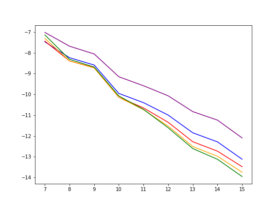
Figure 1: Monte-Carlo (for 30 repeated samples) strong error for different kernel orders: $\log_{2}\mathcal{E}_{N}$ as a function of $\log_{2}N$ for $\ell=1$ (purple), $\ell=3$ (blue), $\ell=5$ (red), $\ell=7$ (orange), $\ell=9$ (green). We see that a polynomial error in $N$ is compatible with the data.

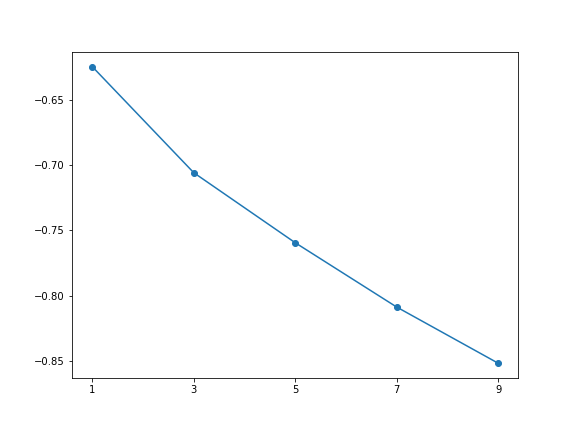
Figure 2: Least-square estimates of the slope $\alpha_{\ell}$ of $\log_{2}\mathcal{E}_{N}=\alpha_{\ell}\log_{2}N+\text{noise}$ in a linear model representation. We plot $\alpha_{\ell}$ as a function of the order $\ell$ of the kernel. We see that a higher order $\ell$ for the choice of the kernel systematically improves on the error rate, as predicted by the statistical bias-variance analysis.

In Figure 1, we display on a log-2 scale $\mathcal{E}_{N}$ for $\ell=1,3,5,7,9$. In Figure 2 we display the least-square estimates of the slope of each curve of Figure 1 according to a linear model. We thus have a proxy of the rate $\alpha_{\ell}$ of the error $\mathcal{E}_{N}\approx N^{-\alpha_{\ell}}$ for different values of $\ell$. We clearly see that higher-order kernels are better suited for estimating $\mu_{t}$. This is of course no surprise from a statistical point of view, but this may have been overlooked in numerical probability simulations.

3.2 A double layer potential

We consider an interaction consisting of a smooth long range attractive and small range repulsive force, obtained as the derivative of double-layer Morse potential. Such models are commonly used (in their kinetic version) in swarming modelling, see for instance [BCC11]. The corresponding McKean-Vlasov equation is

$$dX_{t}=\int_{\mathbb{R}}U^{\prime}(X_{t}-x)\mu_{t}(dx)dt+dB_{t},\;\;\mathcal{L}(X_{0})=\mathcal{N}(0,1),$$

where we pick $U(x)=-\exp(-x^{2})+2\exp(-2x^{2})$. The potential $U$ and its derivative $U^{\prime}$ are displayed in Figure 3.

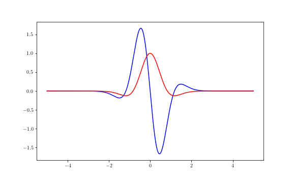
Figure 3: Plot of the potential $U$ (red) and its derivative $U^{\prime}$ (blue).

We implement the Euler scheme $(\bar{X}_{t}^{1,h},\ldots,\bar{X}_{t}^{N,h})_{t\in[0,T]}$ defined in (7) for coefficients $b(x,\mu)=\int_{\mathbb{R}}U^{\prime}(x-y)\mu(dy)$ and $\sigma(t,x)=1$. We pick $T=1$, $h=10^{-2}T=10^{-2}$, for several values of the system size $N=2^{5}=32,2^{6}=64,\ldots,2^{16}=65736$. We then compute

$$\widehat{\mu}_{T}^{N,h,\widehat{\eta}^{N}(T,x)}(x):=N^{-1}\sum_{n=1}^{N}\widehat{\eta}^{N}(T,x)^{-d}K\big{(}\widehat{\eta}^{N}(T,x)^{-1}(x-\bar{X}_{T}^{n,h})\big{)}$$

as our proxy of $\mu_{T}(x)$ for $\ell=1,3,5,7,9$ according to $K$ as in Table 1. The data-driven bandwidth $\widehat{\eta}^{N}(T,x)$ is computed via the minimisation (16), for which one still needs to set the penalty parameter $\varpi$ arising in the Goldenschluger-Lepski method, see (15) in particular. The grid is set as $\mathcal{H}=\{(N/\log N)^{-1/(2m+1)},m=1,\ldots,\ell+1\},$ see in particular Corollary 2.13 in order to mimick the oracle.

In this setting, we do not have access to the exact solution $\mu_{T}(x)$; we nevertheless explore several numerical aspects of our method via the following experiments:

• Investigate the effect of the order $\ell$ of the kernel (for an ad-hoc choice of the penalty parameter $\varpi$). We know beforehand that the mapping $x\mapsto\mu_{T}(x)$ is smooth, and we obtain numerical evidence that a higher-order kernel gives better results by comparing the obtained $\widehat{\mu}_{T}^{N,h,\widehat{\eta}^{N}(T,x)}(x)$ for different values of $\ell$ as $N$ increases in the following sense: for $N=2^{5}$ particles, the estimates for high order kernels are closer to the estimates obtained for $N=2^{10}$ than lower order kernels.

• Investigate the distribution of the data-driven bandwidth $\widehat{\eta}^{N}(T,x)$, for repeated samples as $x$ varies and for different values of the penalty $\varpi$ over the grid $\mathcal{H}=\{(N/\log N)^{-1/(2m+1)},m=1,\ldots,\ell+1\}$. The estimator tends to pick the larger bandwidth with overwhelming probability, which is consistent with our prior knowledge that $x\mapsto\mu_{T}(x)$ is smooth.

• In order to exclude an artifact from the preceding experiment, we conduct a cross-experiment by perturbing the drift with an additional Lipschitz common force (but not smoother) that saturates our Assumption 2.3. This extra transport term lowers down the smoothness of $x\mapsto\mu_{T}(x)$ and by repeating the preceding experiment, we obtain a different distribution of the data-driven bandwidth $\widehat{\eta}^{N}(T,x)$, advocating in favour of a coherent oracle procedure.

The effect of the order $\ell$ of the kernel

We display in Figure 4 the graph of $x\mapsto\widehat{\mu}_{T}^{N,h,\widehat{\eta}^{N}(T,x)}(x)$ for $T=1$, $\ell=1,3,5,7,9$ for $N=2^{5}$ and $N=2^{10}$. The tuning parameter in the choice of $\widehat{\eta}^{N}(T,x)$ is set to $\varpi=23$. The same experiment is displayed in Figure 5 for $N=2^{15}$.

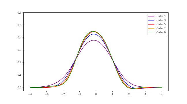
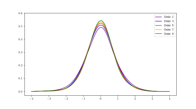
Figure 4: The graph of $x\mapsto\widehat{\mu}_{t}^{N,h,\widehat{\eta}^{N}(t,x)}(x)$. The domain $x\in[-4,4]$ is computed over a discrete grid of $2000$ points, i.e. mesh $4\cdot 10^{-3}$) for $N=2^{5}$ (Left) and $N=2^{10}$ (Right).

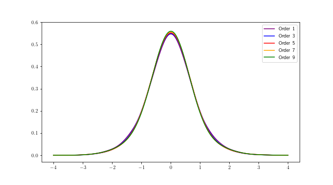
Figure 5: Same experiment as in Figure 4 mimicking an asymptotic behaviour of the procedure for $N=2^{15}$.

The value $N=2^{15}$ mimicks the asymptotic performance of the procedure as compared to $N=2^{5}$ or $N=2^{10}$. We observe that the effect of the order of the kernel $\ell$ is less pronounced. A visual comparison of Figure 4 and 5 suggests that a computation with higher order kernels always perform better, since the shape obtained for $\ell=9$ for small values of $N$ is closer to the asymptotic proxy $N=2^{15}$ than the results obtained with smaller values of $\ell$.

The distribution of the data-driven bandwidth

We pick several values for $\varpi$ (namely $\varpi=20^{-1},10^{-1},1,10,20$) and compute $\widehat{\eta}^{N}(T,x)$ accordingly for $1200$ samples. Figure 6 displays the histogram of the $\widehat{\eta}^{N}(T,x)$ for $x\in[-4,4]$ (discrete grid with mesh $8\cdot 10^{-2}$) for $\ell=3$ and $\ell=5$. We observe that the distribution is peaked around large bandwidths at the far right of the spectrum of the histogram, with comparable results for $\ell=7$ and $\ell=9$. In Figure 7, we repeat the experiment for $\ell=5$ over the restricted domain $[-\tfrac{1}{2},\tfrac{1}{2}]$ (discrete grid, mesh $10^{-2}$) where we expect the solution $\mu_{T}(x)$ to be more concentrated and see no significant difference. This result is in line of course with the statistical nonparametric estimation of a smooth signal (see e.g. the classical textbook [Sil18]).

Cross experiment by reducing the smoothness of $x\mapsto\mu_{T}(x)$

We repeat the previous experiment by adding a perturbation in the drift, via a common force $V^{\prime}(x)=2(1-|x|){\bf 1}_{\{|x|\leq 1\}}$. The drift now becomes $b(x,\mu)=V^{\prime}(x)+\int_{\mathbb{R}}U^{\prime}(x-y)\mu(dy)$. The common transport term $V^{\prime}(x)$ is no smoother than Lipschitz continuous thus reducing the smoothness of the solution $x\mapsto\mu_{T}(x)$. In the same experimental conditions as before, Figure 8 displays the distribution of $\widehat{\eta}^{N}(T,x)$ and is to be compared with Figure 7. We observe that the distribution is modified, in accordance with the behaviour of the oracle bandwidth of a signal with lower order of smoothness. This advocates as further empirical evidence of the coherence of the method.

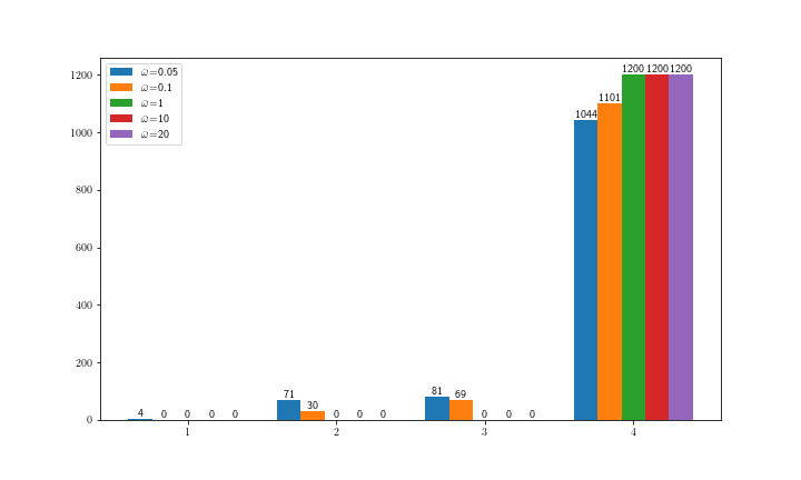
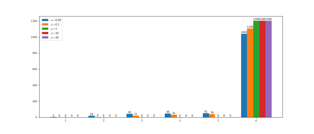
Figure 6: Distribution of $\widehat{\eta}^{N}(T,x)$. The domain $x\in[-4,4]$ is computed over a discrete grid of $100$ points, i.e. mesh $8\cdot 10^{-2}$), $N=2^{5},2^{6},\cdots,2^{16}$ for $\ell=3$ (Top) and $\ell=5$ (Bottom).

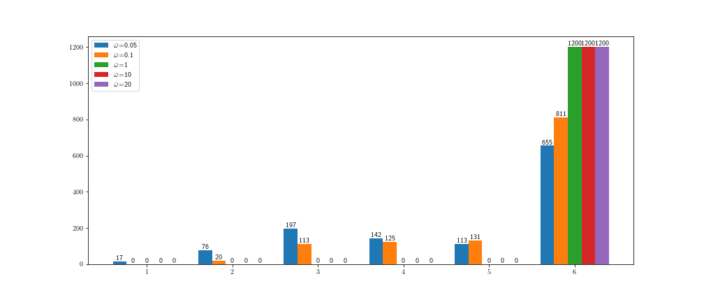
Figure 7: Same experiment as in Figure 6 (Bottom) on the restricted domain $[-\tfrac{1}{2},\tfrac{1}{2}]$ over a discrete grid of $100$ points. The results are comparable with the experiment displayed in Figure 6 (Bottom).

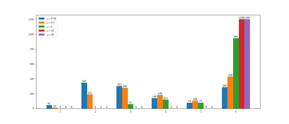
Figure 8: Same experiment as in Figure 7 on the restricted domain $[-\tfrac{1}{2},\tfrac{1}{2}]$ over a discrete grid of $100$ points, when adding a common perturbation force $V^{\prime}(x)=2(1-|x|){\bf 1}_{\{|x|\leq 1\}}$ in the drift. The effect on the empirical distribution of $\widehat{\eta}^{N}(T,x)$ is in line with the behaviour of an oracle bandwidth that adjusts smaller bandwidths when the signal is less smooth.

3.3 The Burgers equation in dimension $d=1$

We consider here the following McKean-Vlasov equation

$$dX_{t}=\int_{\mathbb{R}}H(x-y)\mu_{t}(dy)dt+\sigma dB_{t},\;\;\mathcal{L}(X_{0})=\delta_{0},$$

with $\sigma=\sqrt{0.2}$, associated with the Burgers equation in dimension $d=1$ for $H(x-y)={\bf 1}_{\{y\leq x\}}$. Although the discontinuity at $y=x$ rules out our Assumption 2.3, we may nevertheless implement our method, since a closed form formula is available for $\mu_{t}(x)$. More specifically, for $t>0$, the cumulative density function of $\mu_{t}(x)$ is explicitly given by

$$M_{t}(x)=\frac{\int_{0}^{\infty}\exp\big{(}-\frac{1}{\sigma^{2}}\big{(}\frac{(x-y)^{2}}{2t}+y\big{)}\big{)}dy}{\int_{-\infty}^{0}\exp\big{(}-\frac{1}{\sigma^{2}}\frac{(x-y)^{2}}{2t}\big{)}dy+\int_{0}^{\infty}\exp\big{(}-\frac{1}{\sigma^{2}}\big{(}\frac{(x-y)^{2}}{2t}+y\big{)}\big{)}dy}.$$

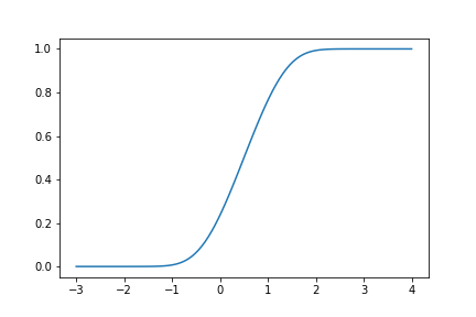
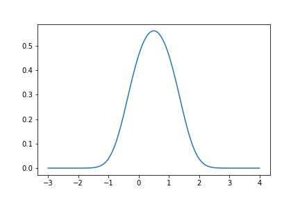
Figure 9: Plots of $x\mapsto M_{T}(x)$ (Left) and $x\mapsto\mu_{T}(x)$ (Right).

Figure 9 displays the graph of $x\mapsto M_{T}(x)$ and $x\mapsto\mu_{T}(x)$ for $T=1$. We display in Figure 10 the reconstruction of $x\mapsto\mu_{T}(x)$ via $\widehat{\mu}_{T}^{N,h,\widehat{\eta}^{N}(T,x)}(x)$ for $N=2^{10}$ for several values of $\ell$. The values $\ell=3$ or $\ell=5$ provide with the best fit, showing again the benefit of higher-order kernels compared to a standard Gaussian kernel (with $\ell=1$). Similar results were obtained for other values of $N$. Yet, the distribution of $\widehat{\eta}^{N}(T,x)$ displayed in Figure 11 shows that our method tends to undersmooth the true density. The effect us less pronounced for $N=2^{15}$. In any case, our numerical results are comparable with [BT97].

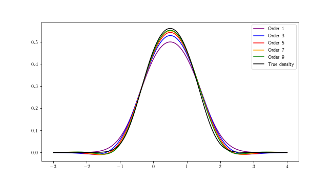
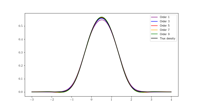
Figure 10: Reconstruction of $\mu_{T}$ by $\widehat{\mu}_{T}^{N,h,\widehat{\eta}^{N}(T,\cdot)}$ with $\varpi=23$, for different kernel orders for $N=2^{10}$ (Top) and $N=2^{15}$ (Bottom). Higher order kernels outperform the reconstruction provided with standard Gaussian kernels ($\ell=1$) for $N=2^{10}$.

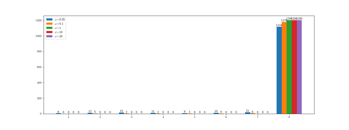
Figure 11: Distribution of $\widehat{\eta}^{N}(T,x)$. The domain $x\in[-3,4]$ is computed for 1200 samples over a discrete grid of $100$ points, i.e. mesh $8\cdot 10^{-2}$, $N=2^{5},2^{6},\ldots,2^{16}$ for $\ell=7$. The method tends pick the largest bandwidth.

4 Proofs

4.1 Proof of Theorem 2.9

We first establish a Bernstein inequality for the fluctuations of $\bar{\mu}_{T}^{N,h}(dx)-\bar{\mu}_{T}^{h}(dx)$.

Proposition 4.1.

Work under Assumptions 2.1, 2.2 and 2.3. Let $N\geq 2$ and $Nh\leq\mathfrak{C}$. For any real-valued bounded function $\varphi$ defined on $\mathbb{R}^{d}$ and any $\varepsilon\geq 0$, we have:

$$\mathbb{P}\Big{(}\int_{\mathbb{R}^{d}}\varphi\,d(\bar{\mu}_{T}^{N,h}-\bar{\mu}_{T}^{h})\geq\varepsilon\Big{)}\leq\kappa_{1}\exp\Big{(}-\frac{\kappa_{2}N\varepsilon^{2}}{|\varphi|^{2}_{L^{2}(\mu_{T})}+|\varphi|_{\infty}\varepsilon}\Big{)},$$ (20)

where $\kappa_{1},\kappa_{2}$ are constants that only depend on $\mathfrak{C}$, $T$ and the data $(\mu_{0},b,\sigma)$ that are explicitly given in the proof.

The proof follows the strategy of Theorem 18 in [DMH21]. We repeat the main steps in order to remain self-contained and highlight the important modifications we need in the context of Euler scheme approximations.

Proof of Proposition 4.1.

We work on a rich enough filtered probability space $(\Omega,\mathcal{F},(\mathcal{F}_{t})_{t\geq 0},\mathbb{P})$ in order to accomodate all the random quantities needed. First, note that the abstract Euler scheme $(\bar{X}^{h}_{t})_{t\in[0,T]}$ defined by (9) solves

$$d\bar{X}^{h}_{t}=b(\underline{t},\bar{X}^{h}_{\underline{t}},{\mu}_{\underline{t}})dt+\sigma(\underline{t},\bar{X}^{h}_{\underline{t}})dB_{t},\quad\mathcal{L}(\bar{X}_{0})=\mu_{0},$$ (21)

where $\underline{t}$ is defined by

$$\forall\;1\leq m\leq M\text{ and }t\in[t_{m},t_{m+1}),\quad\underline{t}\coloneqq t_{m}.$$

Similarly, $(\bar{X}_{t}^{1,h},...,\bar{X}_{t}^{N,h})_{t\in[0,T]}$ defined by (7) solves

$$\begin{cases}d\bar{X}^{n,h}_{t}=b(\underline{t},\bar{X}^{n,h}_{\underline{t}},\bar{\mu}^{N,h}_{\underline{t}})dt+\sigma(\underline{t},\bar{X}^{n,h}_{\underline{t}})dB^{n}_{t},\quad 1\leq n\leq N\\ \bar{\mu}_{\underline{t}}^{N,h}=\frac{1}{N}\sum_{n=1}^{N}\delta_{\bar{X}^{n,h}_{\underline{t}}},\\ \mathcal{L}(\bar{X}_{0}^{1,h},\ldots,\bar{X}_{0}^{N,h})=\mu_{0}^{\otimes N}.\end{cases}$$ (22)

Step 1. We construct a system $(Y_{t}^{1,h},...,Y_{t}^{N,h})_{t\in[0,T]}$ of $N$ independent copies of the abstract Euler schemes (21) (thus without interaction) via

$$\begin{cases}dY_{t}^{n,h}=b(\underline{t},Y_{\underline{t}}^{n,h},\mu_{\underline{t}})dt+\sigma(\underline{t},Y_{\underline{t}}^{n,h})dB_{t}^{n},\quad 1\leq n\leq N\\ (Y_{0}^{1,h},\ldots,Y_{0}^{N,h})=(\bar{X}_{0}^{1,h},\ldots,\bar{X}_{0}^{N,h}),\\ \end{cases}$$ (23)

For $t\in[0,T]$, let

$$L^{N,h}_{t}:=\sum_{n=1}^{N}\int_{0}^{t}\big{(}(c^{-1/2}b)(\underline{s},Y_{\underline{s}}^{n,h},\tfrac{1}{N}\sum_{n=1}^{N}\,\delta_{Y^{n,h}_{\underline{s}}})-(c^{-1/2}b)(\underline{s},Y_{\underline{s}}^{n,h},\mu_{\underline{s}})\big{)}^{\top}dB_{s}^{n}$$

and

$$\mathcal{E}_{t}(L_{\cdot}^{N,h})\coloneqq\exp\big{(}L^{N,h}_{t}-\frac{1}{2}\langle L^{N,h}_{\cdot}\rangle_{t}\big{)},$$

where $c^{-1/2}$ is any square root of $c^{-1}=(\sigma\sigma^{\top})^{-1}$ and $\langle L^{N,h}_{\cdot}\rangle_{t}$ denotes the predictable compensator of $L^{N,h}_{t}$. The following estimate is a key estimate to proceed to a change of probability. Its proof is delayed until the end of this section.

Lemma 4.2.

Work under Assumptions 2.1, 2.2 and 2.3. Assume that $Nh\leq\mathfrak{C}$ for some constant $\mathfrak{C}>0$. For every $\kappa>0$, there exists $\delta(\kappa)>0$ such that

$$\forall\,\delta\in[0,\delta(\kappa)],\quad\quad\,\sup_{t\in[0,T-\delta(\kappa)]}\mathbb{E}_{\mathbb{P}}\Big{[}\exp\Big{(}\kappa\big{(}\langle L_{\cdot}^{N,h}\rangle_{t+\delta}-\langle L_{\cdot}^{N,h}\rangle_{t}\big{)}\Big{)}\Big{]}\leq C^{\prime}$$ (24)

where $C^{\prime}>0$ only depends on $\mathfrak{C}$, $T$ and the data $(\mu_{0},b,\sigma)$.

By taking $\kappa=\frac{1}{2}$ and by applying Novikov’s criterion (see e.g. [KS91, Proposition 3.5.12, Corollary 3.5.13 and 3.5.14]), Lemma 4.2 implies that $\big{(}\mathcal{E}_{t}(L_{\cdot}^{N,h})\big{)}_{t\in[0,T]}$ is a $(\mathcal{F}_{t},\mathbb{P})$ martingale as soon as $Nh\leq\mathfrak{C}$. We may then define another probability distribution $\mathbb{Q}$ on $\big{(}\Omega,\mathcal{F}_{T}\big{)}$ by setting

$$\mathbb{Q}\coloneqq\mathcal{E}_{T}(L^{N,h}_{\cdot})\cdot\mathbb{P}.$$ (25)

By Girsanov’s Theorem (see e.g. [KS91, Theorem 3.5.1]), we have

$$\mathbb{Q}\circ(Y_{t}^{1,h},...,Y_{t}^{N,h})_{t\in[0,T]}^{-1}=\mathbb{P}\circ(X_{t}^{1,h},...,X_{t}^{N,h})_{t\in[0,T]}^{-1}.$$ (26)

Step 2. We claim that for any subdivision $0=t_{0}<t_{1}<...<t_{K}=T$ and for any $\mathcal{F}_{T}$-measurable event $A^{N}$, we have

$$\mathbb{E}\,_{\mathbb{P}}\Big{[}\mathbb{Q}\big{(}A^{N}\;\big{|}\;\mathcal{F}_{t_{j-1}}\big{)}\Big{]}\leq\mathbb{E}\,_{\mathbb{P}}\Big{[}\mathbb{Q}\big{(}A^{N}\;\big{|}\;\mathcal{F}_{t_{j}}\big{)}\Big{]}^{\frac{1}{4}}\mathbb{E}\,_{\mathbb{P}}\Big{[}\exp\Big{(}2\big{(}\langle L_{\cdot}^{N,h}\rangle_{t_{j}}-\langle L_{\cdot}^{N,h}\rangle_{t_{j-1}}\big{)}\Big{)}\Big{]}^{\frac{1}{4}},\>1\leq j\leq K.$$ (27)

The proof is the same as in Step 3 of the proof of Theorem 18 in [DMH21] and is inspired from the estimate (4.2) in Theorem 2.6 in [Lac18]. We repeat the argument: we have

$$\mathbb{E}\,_{\mathbb{P}} \big{[}\mathbb{Q}\big{(}A^{N}\;\big{|}\;\mathcal{F}_{t_{j-1}}\big{)}\big{]}=\mathbb{E}\,_{\mathbb{P}}\big{[}\mathbb{E}\,_{\mathbb{Q}}\big{[}\mathbb{Q}\big{(}A^{N}\;\big{|}\;\mathcal{F}_{t_{j}}\big{)}\;\big{|}\;\mathcal{F}_{t_{j-1}}\big{]}\big{]}$$

$$=\mathbb{E}\,_{\mathbb{P}}\Big{[}\mathbb{E}\,_{\mathbb{P}}\big{[}\,\frac{\,\mathcal{E}_{t_{j}}(L_{\cdot}^{N,h})\,}{\,\mathcal{E}_{t_{j-1}}(L_{\cdot}^{N,h})\,}\,\mathbb{Q}\big{(}A^{N}\;\big{|}\;\mathcal{F}_{t_{j}}\big{)}\;\big{|}\;\mathcal{F}_{t_{j-1}}\big{]}\Big{]}=\mathbb{E}\,_{\mathbb{P}}\Big{[}\,\frac{\,\mathcal{E}_{t_{j}}(L_{\cdot}^{N,h})\,}{\,\mathcal{E}_{t_{j-1}}(L_{\cdot}^{N,h})\,}\,\mathbb{Q}\big{(}A^{N}\;\big{|}\;\mathcal{F}_{t_{j}}\big{)}\Big{]},$$

where the second inequality follows from Bayes’s rule in [KS91, Lemma 3.5.3]. Next, we have

$$\frac{\,\mathcal{E}_{t_{j}}(L_{\cdot}^{N,h})\,}{\,\mathcal{E}_{t_{j-1}}(L_{\cdot}^{N,h})\,}=\mathcal{E}_{t_{j}}\big{(}2(L_{\cdot}^{N,h}-L_{t_{j-1}}^{N,h})\big{)}^{\frac{1}{2}}\cdot\exp\big{(}\langle L_{\cdot}^{N,h}\rangle_{t_{j}}-\langle L_{\cdot}^{N,h}\rangle_{t_{j-1}}\big{)}^{\frac{1}{2}}.$$

The process $\big{(}\mathcal{E}_{t_{j}}\big{(}2(L_{\cdot}^{N,h}-L_{t_{j-1}}^{N,h})\big{)}\big{)}_{t\in[t_{j-1},T]}$ is a $(\mathcal{F}_{t},\mathbb{P})$ martingale if $Nh\leq\mathfrak{C}$. Hence

$$\mathbb{E}\,_{\mathbb{P}}\big{[}\mathcal{E}_{t_{j}}\big{(}2(L_{\cdot}^{N,h}-L_{t_{j-1}}^{N,h})\big{)}\big{]}=1$$

for every $t\in[t_{j-1},T]$. It follows that

$$\mathbb{E}\,_{\mathbb{P}} \Big{[}\mathbb{Q}\big{(}A^{N}\;\big{|}\;\mathcal{F}_{t_{j-1}}\big{)}\Big{]}$$

$$=\mathbb{E}\,_{\mathbb{P}}\left[\,\mathcal{E}_{t_{j}}\big{(}2(L_{\cdot}^{N,h}-L_{t_{j-1}}^{N,h})\big{)}^{\frac{1}{2}}\cdot\exp\big{(}\langle L_{\cdot}^{N,h}\rangle_{t_{j}}-\langle L_{\cdot}^{N,h}\rangle_{t_{j-1}}\big{)}^{\frac{1}{2}}\,\mathbb{Q}\big{(}A^{N}\;\big{|}\;\mathcal{F}_{t_{j}}\big{)}\right]$$

$$\leq\Big{(}\mathbb{E}\,_{\mathbb{P}}\left[\,\exp\big{(}\langle L_{\cdot}^{N,h}\rangle_{t_{j}}-\langle L_{\cdot}^{N,h}\rangle_{t_{j-1}}\big{)}\,\mathbb{Q}\big{(}A^{N}\;\big{|}\;\mathcal{F}_{t_{j}}\big{)}^{2}\right]\Big{)}^{\frac{1}{2}}$$

$$\leq\mathbb{E}\,_{\mathbb{P}}\left[\,\exp\Big{(}2\big{(}\langle L_{\cdot}^{N,h}\rangle_{t_{j}}-\langle L_{\cdot}^{N,h}\rangle_{t_{j-1}}\big{)}\Big{)}\right]^{\frac{1}{4}}\mathbb{E}\,_{\mathbb{P}}\left[\,\mathbb{Q}\big{(}A^{N}\;\big{|}\;\mathcal{F}_{t_{j}}\big{)}^{4}\right]^{\frac{1}{4}}$$

$$\leq\mathbb{E}\,_{\mathbb{P}}\left[\,\exp\Big{(}2\big{(}\langle L_{\cdot}^{N,h}\rangle_{t_{j}}-\langle L_{\cdot}^{N,h}\rangle_{t_{j-1}}\big{)}\Big{)}\right]^{\frac{1}{4}}\mathbb{E}\,_{\mathbb{P}}\left[\,\mathbb{Q}\big{(}A^{N}\;\big{|}\;\mathcal{F}_{t_{j}}\big{)}\right]^{\frac{1}{4}},$$

where the first two inequalities follows from Cauchy-Schwarz’s inequality and the last inequality follows from Jensen’s inequality. Thus (27) is established.

Step 3. Let $A^{N}\in\mathcal{F}_{T}$. Since $\big{(}\mathcal{E}_{t}(L^{N,h}_{\cdot})\big{)}_{t\in[0,T]}$ is a $(\mathcal{F}_{t},\mathbb{P})$ martingale, $\mathbb{P}$ and $\mathbb{Q}$ coincide on $\mathcal{F}_{0}$ (see e.g. [KS91, Section 3 - (5.5)]). It follows that

$$\mathbb{Q}(A^{N})=\mathbb{E}\,_{\mathbb{Q}}\big{[}\,\mathbb{Q}(A^{N}\,\big{|}\,\mathcal{F}_{0})\,\big{]}=\mathbb{E}\,_{\mathbb{P}}\big{[}\,\mathbb{Q}(A^{N}\,\big{|}\,\mathcal{F}_{0})\,\big{]}.$$

Now, let $m\geq 1$ and take a subdivision $0=t_{0}<t_{1}<\ldots<t_{m}=T$ such that

$$\forall\,0\leq k\leq m-1,\quad t_{k+1}-t_{k}\leq\delta(2)$$

where $\delta(2)$ is the constant in Lemma 4.2 for $\kappa=2$. It follows by (27) that

$$\mathbb{E}\,_{\mathbb{P}} \big{[}\,\mathbb{Q}(A^{N}\,\big{|}\,\mathcal{F}_{0})\,\big{]}\leq\mathbb{E}\,_{\mathbb{P}}\big{[}\mathbb{Q}\big{(}A^{N}\;\big{|}\;\mathcal{F}_{T}\big{)}\big{]}^{4^{-m}}\prod_{j=1}^{m}\mathbb{E}\,_{\mathbb{P}}\Big{[}\exp\Big{(}2\big{(}\langle L_{\cdot}^{N,h}\rangle_{t_{j}}-\langle L_{\cdot}^{N,h}\rangle_{t_{j-1}}\big{)}\Big{)}\Big{]}^{\frac{j}{4}}$$

$$\leq\mathbb{P}(A^{N})^{4^{-m}}\prod_{j=1}^{m}\mathbb{E}\,_{\mathbb{P}}\Big{[}\exp\Big{(}2\big{(}\langle L_{\cdot}^{N,h}\rangle_{t_{j}}-\langle L_{\cdot}^{N,h}\rangle_{t_{j-1}}\big{)}\Big{)}\Big{]}^{\frac{j}{4}}\quad\quad\text{(since $A^{N}\in\mathcal{F}_{T}$)}$$

$$\leq\mathbb{P}(A^{N})^{4^{-m}}\Big{(}\sup_{t\in[0,T-\delta(2)]}\mathbb{E}_{\mathbb{P}}\Big{[}\exp\Big{(}2\big{(}\langle L_{\cdot}^{N,h}\rangle_{t+\varepsilon}-\langle L_{\cdot}^{N,h}\rangle_{t}\big{)}\Big{)}\Big{]}\Big{)}^{\frac{m(m+1)}{8}}$$

$$\leq\mathbb{P}(A^{N})^{4^{-m}}C^{\prime\frac{m(m+1)}{8}}$$ (28)

by applying Lemma 4.2 with $\kappa=2$.

Step 4. We first recall the Bernstein’s inequality: if $Z_{1},\ldots,Z_{N}$ are real-valued centred independent random variables bounded by some constant $Q$, we have

$$\forall\,\varepsilon\geq 0,\quad\quad\mathbb{P}\Big{(}\sum_{n=1}^{N}Z_{n}\geq\varepsilon\Big{)}\leq\exp\Big{(}\;-\;\frac{\varepsilon^{2}}{\,2\sum_{n=1}^{N}\mathbb{E}\,[Z_{n}^{2}]+\frac{2}{3}Q\varepsilon}\Big{)}.$$ (29)

Now, for $\varepsilon\geq 0$, we pick

$$A^{N}_{T}\coloneqq \Big{\{}\sum_{n=1}^{N}\Big{(}\varphi\big{(}Y_{T}^{n,h}\big{)}-\int_{\mathbb{R}^{d}}\varphi(y)\bar{\mu}_{T}^{h}(dy)\Big{)}\geq N\varepsilon\Big{\}}$$

so that $A^{N}_{T}\in\mathcal{F}_{T}$. Since $(Y_{T}^{1,h},\ldots,Y_{T}^{N,h})$ are independent with common distribution $\bar{\mu}_{T}^{h}$, we have

$$\mathbb{P}(A^{N}_{T})\leq\exp\Big{(}\;-\;\frac{N\varepsilon^{2}}{\,2|\varphi|_{L^{2}(\bar{\mu}_{T})}^{2}+\frac{2}{3}|\varphi|_{\infty}\varepsilon\,}\Big{)}.$$ (30)

by (29) with $Z_{n}=\varphi(Y_{T}^{n,h})-\int_{\mathbb{R}^{d}}\varphi(x)\bar{\mu}_{T}^{h}(dx)$, having $\mathbb{E}\,[Z_{n}^{2}]\leq|\varphi|_{L^{2}(\bar{\mu}_{T}^{h})}^{2}$ and $Q=|\varphi|_{\infty}$. It follows by (26) that

$$\mathbb{P}\Big{(}\int_{\mathbb{R}^{d}}\varphi\,d(\bar{\mu}_{T}^{N,h}-\bar{\mu}_{T}^{h})\geq\varepsilon\Big{)}=\mathbb{P}\Big{(}\sum_{n=1}^{N}\Big{(}\varphi\big{(}\bar{X}_{T}^{n,h}\big{)}-\int_{\mathbb{R}}\varphi(y)\bar{\mu}_{T}^{h}(dy)\Big{)}\geq N\varepsilon\Big{)}=\mathbb{Q}(A^{N}_{T}).$$

By Step 3, we infer

$$\mathbb{Q}(A^{N}_{T}) \leq\mathbb{P}(A^{N}_{T})^{4^{-m}}C^{\prime\frac{m(m+1)}{8}}\leq C^{\prime\frac{m(m+1)}{8}}\exp\Big{(}-4^{-m}\frac{N\varepsilon^{2}}{2|\varphi|_{L^{2}(\bar{\mu}_{T}^{h})}^{2}+\frac{2}{3}|\varphi|_{\infty}\varepsilon\,}\Big{)},$$

and we conclude by taking $\kappa_{1}=C^{\prime\frac{m(m+1)}{8}}$ and $\kappa_{2}=2^{-1}4^{-m}$. ∎

Completion of proof of Theorem 2.9

Recall the notation $K_{\eta}(x)=\eta^{-d}K(\eta^{-1}x)$ and set $\varphi\star\psi(x)=\int_{\mathbb{R}^{d}}\varphi(x-y)\psi(y)dy$ for the convolution product between two integrable functions $\varphi,\psi:\mathbb{R}^{d}\rightarrow\mathbb{R}$. We have

$$\mathbb{P}\big{(}\big{|}\widehat{\mu}_{T}^{N,h,\eta}(x)-\mu_{T}(x)\big{|}\geq\varepsilon\big{)}$$

$$\leq\mathbb{P}\big{(}\big{|}\widehat{\mu}^{N,h,\eta}_{T}(x)-K_{\eta}\star\bar{\mu}^{h}_{T}(x)\big{|}\geq\varepsilon/3\big{)}+{\bf 1}_{\{|K_{\eta}\star\bar{\mu}^{h}_{T}(x)-K_{\eta}\star\mu_{T}(x)|\geq\varepsilon/3\}}+{\bf 1}_{\{|K_{\eta}\star\mu_{T}(x)-\mu_{T}(x)|\geq\varepsilon/3\}}.$$ (31)

We have

$$\big{|}K_{\eta}\star\bar{\mu}^{h}_{T}(x)-K_{\eta}\star\mu_{T}(x)\big{|}\leq|K|_{L^{1}}\sup_{x\in\mathbb{R}^{d}}\big{|}\bar{\mu}_{T}^{h}(x)-\mu_{T}(x)\big{|}$$

since $|K_{\eta}|_{L^{1}}=|K|_{L^{1}}$ and this last term is strictly smaller than $\varepsilon/3$ for $h<h\big{(}|K|_{L^{1}}^{-1}\tfrac{1}{3}\varepsilon\big{)}$, therefore the second indicator is $0$. Likewise

$$\big{|}K_{\eta}\star\mu_{T}(x)-\mu_{T}(x)\big{|}\leq\mathcal{B}_{\eta}(\mu_{T},x)<\varepsilon/3$$

for $\eta<\eta(\tfrac{1}{3}\varepsilon)$ and the third indicator is $0$ as well. Finally

$$\mathbb{P}\Big{(}\big{|}\widehat{\mu}^{N,h,\eta}_{T}(x)-K_{\eta}\star\bar{\mu}^{h}_{T}(x)\big{|}\geq\tfrac{1}{3}\varepsilon\Big{)}$$

$$=\mathbb{P}\Big{(}\big{|}\int_{\mathbb{R}^{d}}K_{\eta}(x-\cdot)d(\bar{\mu}^{N,h}_{T}-\bar{\mu}^{h}_{T})\big{|}\geq\tfrac{1}{3}\varepsilon\Big{)}\leq 2\kappa_{1}\exp\Big{(}-\frac{\kappa_{2}N(\tfrac{1}{3}\varepsilon)^{2}}{|K_{\eta}(x-\cdot)|^{2}_{L^{2}(\mu_{T})}+|K_{\eta}|_{\infty}\varepsilon}\Big{)}$$

by Proposition 4.1 and Theorem 2.9 follows.

Proof of Lemma 4.2

Writing $\widetilde{\mu}^{N,h}_{s}=\tfrac{1}{N}\sum_{n=1}^{N}\,\delta_{Y^{n,h}_{s}}$, for $\kappa>0$, we have

$$\kappa\big{(}\langle L_{\cdot}^{N,h}\rangle_{t+\delta}-\langle L_{\cdot}^{N,h}\rangle_{t}\big{)}$$

$$=\kappa\sum_{n=1}^{N}\int_{t}^{t+\delta}\big{(}b(\underline{s},Y_{\underline{s}}^{n,h},\widetilde{\mu}^{N,h}_{\underline{s}})-b(\underline{s},Y_{\underline{s}}^{n,h},\mu_{\underline{s}})\big{)}^{\top}c(\underline{s},Y_{\underline{s}}^{n,h})^{-1}\big{(}b(\underline{s},Y_{\underline{s}}^{n,h},\widetilde{\mu}^{N,h}_{\underline{s}})-b(\underline{s},Y_{\underline{s}}^{n,h},\mu_{\underline{s}})\big{)}ds$$

$$\leq\kappa\sup_{t\in[0,T]}|\mathrm{Tr}(c(t,\cdot)^{-1})|_{\infty}\sum_{n=1}^{N}\int_{t}^{t+\delta}\big{|}b(\underline{s},Y_{\underline{s}}^{n,h},\widetilde{\mu}^{N,h}_{\underline{s}})-b(\underline{s},Y_{\underline{s}}^{n,h},\mu_{\underline{s}})\big{|}^{2}ds$$

$$\leq 2\kappa\sup_{t\in[0,T]}|\mathrm{Tr}(c(t,\cdot)^{-1})|_{\infty}\Big{(}\sum_{n=1}^{N}\int_{t}^{t+\delta}\big{|}b(\underline{s},Y_{\underline{s}}^{n,h},\widetilde{\mu}^{N,h}_{\underline{s}})-b(\underline{s},Y_{\underline{s}}^{n,h},\bar{\mu}_{\underline{s}}^{h})\big{|}^{2}ds$$

$$\hskip 170.71652pt+N|\widetilde{b}|_{\mathrm{Lip}}^{2}\int_{t}^{t+\delta}\mathcal{W}_{1}(\bar{\mu}_{\underline{s}}^{h},\mu_{\underline{s}})^{2}ds\Big{)},$$

by the uniform ellipticity of $c$ thanks to Assumption 2.2 and by triangle inequality for the last inequality, with $|\widetilde{b}(t,x,y)-\widetilde{b}(t,x,y^{\prime})\big{|}\leq|\widetilde{b}|_{\mathrm{Lip}}|y-y^{\prime}|$ in particular. Recall that under Assumption 2.1, 2.2 and 2.3, there exists a unique strong solution $X=(X_{t})_{t\in[0,T]}$ of the McKean-Vlasov equation (2) satisfying

$$\forall\,s,t\in[0,T],s<t,\qquad\mathbb{E}\big{[}|X_{t}-X_{s}|^{2}\big{]}^{1/2}\leq\bar{\kappa}\sqrt{t-s}$$

for some $\bar{\kappa}$ that depends on $(\mu_{0},b,\sigma)$ and $T$, see [LP23, Proposition 2.1]. Hence, the function $(t,x)\mapsto b^{\,\mu}(t,x)\coloneqq b(t,x,\mu_{t})$ with $\mu_{t}=\mathcal{L}(X_{t})$ is $\frac{1}{2}$-Hölder continuous in $t$ and Lipschitz continuous in $x$. Thus, one can obtain

$$\sup_{s\in[0,T]}\mathcal{W}_{1}(\bar{\mu}_{\underline{s}}^{h},\mu_{\underline{s}})\leq\kappa_{7}h^{1/2},$$

where $\kappa_{7}$ depends on the data $(\mu_{0},b,\sigma)$ and $T$, by rewriting (2) as a Brownian diffusion

$$dX_{t}=b^{\,\mu}(t,X_{t})dt+\sigma(t,X_{t})dB_{t}$$

and by applying the classical convergence result of the Euler scheme for a Brownian diffusion (see e.g. [Pag18, Theorem 7.2]) since for every $s\in[0,T]$, $\mathcal{W}_{1}(\bar{\mu}_{s}^{h},\mu_{s})\leq\mathbb{E}\big{[}|X_{s}-\bar{X}_{s}^{h}|\big{]}$. Writing

$$b(\underline{s},Y_{\underline{s}}^{n,h},\widetilde{\mu}^{N,h}_{\underline{s}})-b(\underline{s},Y_{\underline{s}}^{n,h},\bar{\mu}_{\underline{s}}^{h}) =N^{-1}\sum_{n^{\prime}=1}^{N}\xi_{s}^{n,n^{\prime}}=N^{-1}\xi_{s}^{n,n}+\tfrac{N-1}{N}S_{s}^{n,N},$$

with $S_{s}^{n,N}=\tfrac{1}{N-1}\sum_{n^{\prime}\neq n}\xi_{s}^{n,n^{\prime}}$ and

$$\xi_{s}^{n,n^{\prime}}=\widetilde{b}(\underline{s},Y_{\underline{s}}^{n,h},Y_{\underline{s}}^{n^{\prime},h})-\int_{\mathbb{R}^{d}}\widetilde{b}(\underline{s},Y_{\underline{s}}^{n,h},y)\bar{\mu}_{\underline{s}}^{h}(dy).$$

The random variables $(\xi_{s}^{n,n^{\prime}})_{1\leq n^{\prime}\leq N,n^{\prime}\neq n}$ are centered, identically distributed and conditionally independent given $Y_{\underline{s}}^{n,h}$. Moreover, for every integer $m\geq 1$, we have the following estimate

Lemma 4.3.

We have

$$\sup_{s\in[0,T]}\mathbb{E}\big{[}|Y_{\underline{s}}^{n,h}|^{2m}\big{]}\leq\kappa_{8}^{m}m!$$

where $\kappa_{8}>0$ depends on $T$ and the data $(\mu_{0},b,\sigma)$.

The proof is standard (see for instance [Mél96, Szn91] or [DMH21] for a control of growth in the constant $m$ and we omit it). From Lemma 4.3, we infer, for every $m\geq 1$:

$$\mathbb{E}\Big{[}\big{|}\xi_{s}^{n,n^{\prime}}\big{|}^{2m}\,|\,Y_{\underline{s}}^{n,h}\Big{]}=\mathbb{E}\,\Big{[}\;\big{|}\widetilde{b}(\underline{s},Y_{\underline{s}}^{n,h},Y_{\underline{s}}^{n^{\prime},h})-\int_{\mathbb{R}^{d}}\widetilde{b}(\underline{s},Y_{\underline{s}}^{n,h},y)\bar{\mu}_{\underline{s}}^{h}(dy)\big{|}^{2m}\;\Big{|}\;Y_{\underline{s}}^{n,h}\;\Big{]}$$

$$\quad\leq\mathbb{E}\,\Big{[}\;2^{2m-1}\Big{(}\big{|}\widetilde{b}(\underline{s},Y_{\underline{s}}^{n,h},Y_{\underline{s}}^{n^{\prime},h})-\widetilde{b}(\underline{s},Y_{\underline{s}}^{n,h},0)\big{|}^{2m}$$

$$\quad\qquad+\big{|}\widetilde{b}(\underline{s},Y_{\underline{s}}^{n,h},0)-\int_{\mathbb{R}^{d}}\widetilde{b}(\underline{s},Y_{\underline{s}}^{n,h},y)\bar{\mu}_{\underline{s}}^{h}(dy)\big{|}^{2m}\Big{)}\;\Big{|}\;Y_{\underline{s}}^{n,h}\;\Big{]}$$

$$\quad\leq\mathbb{E}\,\Big{[}\;2^{2m-1}\Big{(}\;|\widetilde{b}|_{\mathrm{Lip}}^{2m}\,|Y_{\underline{s}}^{n^{\prime},h}|^{2m}+|\widetilde{b}|_{\mathrm{Lip}}^{2m}\,\mathbb{E}\,\big{[}|Y_{\underline{s}}^{n^{\prime},h}|^{2m}\big{]}\;\Big{)}\;\Big{|}\;Y_{\underline{s}}^{n,h}\;\Big{]}=2^{2m}\,|\widetilde{b}|_{\mathrm{Lip}}^{2m}\,\mathbb{E}\,\big{[}|Y_{\underline{s}}^{n^{\prime},h}|^{2m}\big{]}$$

$$\quad\leq\big{(}4|\widetilde{b}|_{\mathrm{Lip}}^{2}\kappa_{8}\big{)}^{m}m!$$

and in turn, by letting $\kappa_{9}=24|\widetilde{b}|_{\mathrm{Lip}}^{2}\kappa_{8}$, we derive, for every $v\in\mathbb{R}$,

$$\mathbb{E}\big{[}\exp(v(\xi_{s}^{n,n^{\prime}})_{[k]})\,|\,Y_{\underline{s}}^{n,h}\big{]}\leq\exp\big{(}\tfrac{\kappa_{9}v^{2}}{2}\big{)},\;\;k=1,\ldots,d.$$

In other words, conditional on $Y_{\underline{s}}^{n,h}$, each component $(\xi_{s}^{n,n^{\prime}})_{[k]}$ of $\xi_{s}^{n,n^{\prime}}=\big{(}(\xi_{s}^{n,n^{\prime}})_{[1]},\ldots,(\xi_{s}^{n,n^{\prime}})_{[d]}\big{)}$ is sub-Gaussian with variance proxy $\kappa_{9}$ (see e.g. [BK80] and [Pau20, Theorem 2.1.1]). Consequently, conditional on $Y_{\underline{s}}^{n,h}$, each component $(S_{s}^{n,N})_{[k]}$ of $S_{s}^{n,N}$ is sub-Gaussian with variance proxy $(N-1)^{-1}\kappa_{9}$, by the conditional independence of the random variables $(\xi_{s}^{n,n^{\prime}})_{1\leq n^{\prime}\leq N,n^{\prime}\neq n}$. This implies in particular

$$\mathbb{E}\Big{[}\exp\Big{(}\frac{(N-1)(S_{s}^{n,N})_{[k]}^{2}}{8\kappa_{9}}\Big{)}\Big{]}=\mathbb{E}\Big{[}\,\mathbb{E}\Big{[}\exp\Big{(}\frac{(N-1)(S_{s}^{n,N})_{[k]}^{2}}{8\kappa_{9}}\Big{)}\;\Big{|}\;Y_{\underline{s}}^{n,h}\Big{]}\,\Big{]}\color[rgb]{0,0,0}\leq 2,$$

and in turn

$$\mathbb{E}\Big{[}\exp\Big{(}\frac{(N-1)|S_{s}^{n,N}|^{2}}{8d\kappa_{9}}\Big{)}\Big{]}\leq d^{-1}\sum_{k=1}^{d}\mathbb{E}\Big{[}\exp\Big{(}\frac{(N-1)(S_{s}^{n,N})_{[k]}^{2}}{8\kappa_{9}}\Big{)}\Big{]}\leq 2.$$ (32)

Likewise

$$\mathbb{E}\Big{[}\exp\Big{(}\frac{|\xi_{s}^{n,n}|^{2}}{8d\kappa_{9}}\Big{)}\Big{]}\leq 2.$$ (33)

Abbreviating $\tau=2\kappa\sup_{t\in[0,T]}|\mathrm{Tr}(c(t,\cdot)^{-1})|_{\infty}$, it follows that

$$\mathbb{E}\Big{[}\exp\big{(}\kappa(\langle L_{\cdot}^{N,h}\rangle_{t+\delta}-\langle L_{\cdot}^{N,h}\rangle_{t})\big{)}\Big{]}$$

$$\leq e^{\tau|\widetilde{b}|_{\mathrm{Lip}}^{2}\kappa_{7}^{2}\delta Nh}\mathbb{E}\Big{[}\exp\Big{(}\tau\int_{t}^{t+\delta}\sum_{n=1}^{N}\big{|}N^{-1}\sum_{n^{\prime}=1}^{N}\xi_{s}^{n,n^{\prime}}\big{|}^{2}ds\Big{)}\Big{]}$$

$$\leq e^{\tau|\widetilde{b}|_{\mathrm{Lip}}^{2}\kappa_{7}^{2}\delta Nh}\tfrac{1}{2\delta}\int_{t}^{t+\delta}N^{-1}\sum_{n=1}^{N}\Big{(}\mathbb{E}\Big{[}\exp\big{(}4\delta\tau N\big{|}N^{-1}\xi_{s}^{n,n}\big{|}^{2}\big{)}\Big{]}+\mathbb{E}\Big{[}\exp\big{(}4\tau\delta N\big{|}\tfrac{N-1}{N}S_{s}^{n,N}\big{|}^{2}\big{)}\Big{]}\Big{)}ds$$

$$\leq 2e^{\tau|\widetilde{b}|_{\mathrm{Lip}}^{2}\kappa_{7}^{2}\delta Nh}$$

as soon as $\delta\leq(32\tau d\kappa_{9})^{-1}\tfrac{N}{N-1}=(64\kappa\sup_{t\in[0,T]}|\mathrm{Tr}(c(t,\cdot)^{-1})|_{\infty}d\kappa_{9})^{-1}\tfrac{N}{N-1}$ by (32) and (33). We obtain Lemma 4.2 with $C^{\prime}=2\exp(\kappa_{10}\mathfrak{C})$ with $\kappa_{10}=\frac{\kappa_{7}^{2}}{384d\kappa_{8}}$.

4.2 Proof of Theorem 2.10

We first need a crucial approximation result of the density of a diffusion process by the density of its Euler scheme counterpart. We heavily rely on the sharp results of Gobet and Labart [GL08a].

Proposition 4.4.

Work under Assumptions 2.1, 2.2 and 2.3. For any $0<t_{\min}\leq T$, we have

$$\sup_{(t,x)\in[t_{\min},T]\times\mathbb{R}^{d}}\big{|}\bar{\mu}^{h}_{t}(x)-\mu_{t}(x)\big{|}\leq\kappa_{10}\cdot h,$$ (34)

for some $\kappa_{10}>0$ depending on $t_{\min},T,d$ and the data $(\mu_{0},b,\sigma)$.

Proof.

For $x_{0}\in\mathbb{R}^{d}$, let $(\xi_{t}^{x_{0}})_{t\in[0,T]}$ be a diffusion process of the form

$$\xi_{t}^{x_{0}}=x_{0}+\int_{0}^{t}\tilde{b}(s,\xi_{s}^{x_{0}})ds+\int_{0}^{t}\tilde{\sigma}(s,\xi_{s}^{x_{0}})dB_{s},$$ (35)

where $\widetilde{\sigma}:[0,T]\times\mathbb{R}^{d}\rightarrow\mathbb{R}^{d}\otimes\mathbb{R}^{d}$ and $\widetilde{b}:[0,T]\times\mathbb{R}^{d}\rightarrow\mathbb{R}^{d}$ are both $\mathcal{C}^{1,3}_{b}$ and $\widetilde{\sigma}$ is uniformly elliptic and $\partial_{t}\widetilde{\sigma}$ is $\mathcal{C}_{b}^{0,1}$. We associate its companion Euler scheme $(\bar{\xi}_{t}^{x_{0},h})_{t\in[0,T]}$:

$$\begin{cases}\bar{\xi}_{t_{m+1}}^{x_{0},h}=\bar{\xi}_{t_{m}}^{x_{0},h}+h\cdot\tilde{b}(t_{m},\bar{\xi}^{x_{0},h}_{t_{m}})+\sqrt{h}\,\tilde{\sigma}(t_{m},\bar{\xi}_{t_{m}}^{x_{0},h})Z_{m+1},\\ Z_{m+1}^{n}\coloneqq\frac{1}{\sqrt{h}}\big{(}B_{t_{m+1}}-B_{t_{m}}\big{)},\noindent\\ \bar{\xi}_{t_{0}}^{x_{0},h}=x_{0},\\ \forall\,t\in[t_{m},t_{m+1}),\quad\bar{\xi}_{t}^{x_{0},h}=\bar{\xi}_{t_{m}}^{x_{0},h}+(t-t_{m})\tilde{b}(t_{m},\bar{\xi}_{t_{m}}^{x_{0},h})+\tilde{\sigma}(t_{m},\bar{\xi}_{t_{m}}^{x_{0},h})(B_{t}-B_{t_{m}}).\end{cases}$$

For $t>0$, both $\mathcal{L}(\xi_{t}^{x_{0}})$ and $\mathcal{L}(\bar{\xi}_{t}^{x_{0},h})$ are absolutely continuous, with density $p_{t}(x_{0},x)$ and $\bar{p}_{t}^{h}(x_{0},x)$ w.r.t. the Lebesgue measure $dx$ on $\mathbb{R}^{d}$. By Theorem 2.3 in [GL08a], there exist two constants $c_{1}$ and $c_{2}$ depending on $T$, $d$ and the data $(\widetilde{\sigma},\widetilde{b})$ such that

$$\big{|}\bar{p}^{h}_{t}(x_{0},x)-p_{t}(x_{0},x)\big{|}\leq c_{1}h\,t^{-\frac{d+1}{2}}\exp\Big{(}-\frac{c_{2}|x-x_{0}|^{2}}{t}\Big{)}.$$ (36)

Taking $\widetilde{\sigma}(t,x)=\sigma(t,x)$ and $\widetilde{b}(t,x)=b(t,x,\mu_{t})$, we can identify $\bar{\mu}_{t}(x)$ with $\int_{\mathbb{R}^{d}}\bar{p}_{t}^{h}(x_{0},x)\mu_{0}(dx_{0})$ and $\mu_{t}(x)$ with $\int_{\mathbb{R}^{d}}p_{t}(x_{0},x)\mu_{0}(dx_{0})$. For every $t\in[t_{\min},T]$, we have

$$\big{|}\bar{\mu}_{t}^{h}(x)-\mu_{t}(x)\big{|} \leq\int_{\mathbb{R}^{d}}\big{|}\bar{p}_{t}^{h}(x_{0},x)-p_{t}(x_{0},x)\big{|}\mu_{0}(dx_{0})$$

$$\leq c_{1}h\int_{\mathbb{R}^{d}}\,t^{-\frac{d+1}{2}}\exp\Big{(}-\frac{c_{2}|x-x_{0}|^{2}}{t}\Big{)}\mu_{0}(dx_{0})$$

$$\leq c_{1}t_{\min}^{-\frac{d+1}{2}}\cdot h=:\kappa_{10}\cdot h,$$

by Theorem 2.3 in [GL08a] since Assumption 2.3 implies $(t,x)\mapsto b(t,x,\mu_{t})$ is $\mathcal{C}_{b}^{1,3}$. More specifically, for $(X_{t})_{t\in[0,T]}$ solving (2), we have

$$b(t,x,\mu_{t})=\mathbb{E}\big{[}\,\widetilde{b}(t,x,X_{t})\big{]}.$$

By dominated convergence, $x\mapsto b(t,x,\mu_{t})$ is $\mathcal{C}^{3}_{b}$ thanks to the regularity assumptions on $x\mapsto\widetilde{b}(t,x,y)$. For the regularity in time, by Itô’s formula

$$\mathbb{E}\big{[}\,\widetilde{b}(t,\cdot,X_{t})\big{]} =\mathbb{E}\big{[}\,\widetilde{b}(0,\cdot,X_{0})\big{]}+\int_{0}^{t}\mathbb{E}\big{[}\partial_{T}\widetilde{b}(s,\cdot,X_{s})\big{]}ds+\int_{0}^{t}\mathbb{E}\big{[}\mathcal{A}_{s}\widetilde{b}(s,\cdot,X_{s})\big{]}ds,$$

where $(\mathcal{A}_{s})_{s\in[0,T]}$ is the family of generators defined in (18) applied to

$$y\mapsto\widetilde{b}(s,\cdot,y)=(\widetilde{b}(s,\cdot,y)_{[1]},\ldots,\widetilde{b}(s,\cdot,y)_{[d]})$$

componentwise. Moreover, for each component $1\leq k\leq d$,

$$\mathcal{A}_{s}\widetilde{b}(s,\cdot,X_{s})_{[k]} =\mathbb{E}\big{[}\,\widetilde{b}(s,\cdot,X_{s})]^{\top}\nabla_{y}\widetilde{b}(s,\cdot,X_{s})_{[k]}+\tfrac{1}{2}\sum_{l,l^{\prime}=1}^{d}c_{ll^{\prime}}(s,X_{s})\partial_{y_{l}y_{l^{\prime}}}\widetilde{b}(s,\cdot,X_{s})_{[k]},$$

hence

$$\mathbb{E}\big{[}\mathcal{A}_{s}\widetilde{b}(s,\cdot,X_{s})_{[k]}\big{]}=\mathbb{E}\big{[}\,\widetilde{b}(s,\cdot,X_{s})]^{\top}\mathbb{E}\big{[}F_{k}(s,X_{s})\big{]}+\mathbb{E}\big{[}G_{k}(s,X_{s})\big{]},$$

with

$$F_{k}(s,y)=\nabla_{y}\widetilde{b}(s,\cdot,y)_{[k]},\;\;\text{and}\;\;G_{k}(s,y)=\tfrac{1}{2}\sum_{l,l^{\prime}=1}^{d}c_{ll^{\prime}}(s,y)\partial_{y_{l}y_{l^{\prime}}}\widetilde{b}(s,\cdot,y)_{[k]}.$$

All three functions $(s,y)\mapsto\widetilde{b}(s,\cdot,y)$, $(s,y)\mapsto F_{k}(s,y)$ and $(s,y)\mapsto G_{k}(s,y)$ are continuous and bounded by Assumption 2.3, and so are $s\mapsto\mathbb{E}\big{[}\,\widetilde{b}(s,\cdot,X_{s})]$, $s\mapsto\mathbb{E}\big{[}F_{k}(s,X_{s})\big{]}$ and $s\mapsto\mathbb{E}\big{[}G_{k}(s,X_{s})\big{]}$ by dominated convergence using in particular that $s\mapsto X_{s}$ is stochastically continuous. Hence $s\mapsto\mathbb{E}\big{[}\mathcal{A}_{s}\widetilde{b}(s,\cdot,X_{s})\big{]}$ is continuous and $s\mapsto\mathbb{E}\big{[}\partial_{s}\widetilde{b}(s,\cdot,X_{s})\big{]}$ too, using again Assumption 2.3. It follows that $t\mapsto b(t,x,\mu_{t})$ is $\mathcal{C}_{b}^{1}$ on $[0,T]$. ∎

Completion of proof of Theorem 2.10

We have

$$\mathbb{E}\big{[}\big{|}\widehat{\mu}^{N,h,\eta}_{T}(x)-\mu_{T}(x)\big{|}^{p}\big{]} \leq 3^{p-1}\Big{(}\mathbb{E}\big{[}\big{|}\widehat{\mu}^{N,h,\eta}_{T}(x)-K_{\eta}\star\bar{\mu}^{h}_{T}(x)\big{|}^{p}\big{]}$$

$$\hskip 8.53581pt+\big{|}K_{\eta}\star\bar{\mu}^{h}_{T}(x)-K_{\eta}\star\mu_{T}(x)\big{|}^{p}+\big{|}K_{\eta}\star\mu_{T}(x)-\mu_{T}(x)\big{|}^{p}\Big{)},$$

and we plan to bound each term separately. First, by Proposition 4.1

$$\mathbb{E}\big{[}\big{|}\widehat{\mu}^{N,h,\eta}_{T}(x)-K_{\eta}\star\bar{\mu}^{h}_{T}(x)\big{|}^{p}\big{]} =\int_{0}^{\infty}\mathbb{P}\big{(}\big{|}\widehat{\mu}^{N,h,\eta}_{T}(x)-K_{\eta}\star\bar{\mu}^{h}_{T}(x)\big{|}\geq z^{1/p}\big{)}\,dz$$

$$\leq 2\kappa_{1}\int_{0}^{\infty}\exp\Big{(}-\frac{\kappa_{2}Nz^{2/p}}{|K_{\eta}(x-\cdot)|^{2}_{L^{2}(\mu_{T})}+|K_{\eta}|_{\infty}z^{1/p}}\Big{)}\,dz$$

$$\leq 2\kappa_{1}\int_{0}^{\infty}\exp\Big{(}-\frac{\kappa_{2}N\eta^{d}z^{2/p}}{\sup_{y\in\mathrm{Supp}(K)}\mu_{T}(x-y)|K|^{2}_{L^{2}}+|K|_{\infty}z^{1/p}}\Big{)}\,dz$$

$$\leq 2\kappa_{1}c_{p}\kappa_{2}^{-p/2}\sup_{y\in\mathrm{Supp}(K)}\mu_{T}(x-y)^{p/2}|K|^{p}_{L^{2}}(N\eta^{d})^{-p/2},$$

stemming from the estimate

$$\int_{0}^{\infty}\exp\Big{(}-\frac{az^{2/p}}{b+cz^{1/p}}\Big{)}dz\leq c_{p}\max\Big{(}\Big{(}\frac{a}{b}\Big{)}^{-p/2},\Big{(}\frac{a}{c}\Big{)}^{-p}\Big{)},$$

valid for $a,b,c,p>0$, with $c_{p}=2\int_{0}^{\infty}\exp\big{(}-\tfrac{1}{2}(\min(z,\sqrt{z}))^{2/p}\big{)}dz$. Next,

$$\big{|}K_{\eta}\star\bar{\mu}^{h}_{T}(x)-K_{\eta}\star\mu_{T}(x)\big{|}^{p} \leq\sup_{y\in\mathbb{R}^{d}}\big{|}\bar{\mu}_{T}^{h}(y)-\mu_{T}(y)\big{|}^{p}\big{(}\int_{\mathbb{R}^{d}}\big{|}K_{\eta}(x-y)\big{|}dy\big{)}^{p}\leq\kappa^{p}_{10}|K|_{L^{1}}^{p}h^{p}$$

by Proposition 4.4. Finally, by definition

$$\big{|}K_{\eta}\star\mu_{T}(x)-\mu_{T}(x)\big{|}^{p}\leq\mathcal{B}_{\eta}(\mu_{T},x)^{p},$$

and we obtain Theorem 2.10 with

$$\kappa_{3}=3^{p-1}\max\big{(}2\kappa_{1}c_{p}\kappa_{2}^{-p/2}\sup_{y\in\mathrm{Supp}(K)}\mu_{T}(x-y)^{p/2}|K|^{p}_{L^{2}},\kappa^{p}_{10}|K|_{L^{1}}^{p},1\big{)}.$$

Proof of Corollary 2.11

By Taylor’s formula, we have, for $x,y\in\mathbb{R}^{d}$, $\eta>0$ and any $1\leq k^{\prime}\leq k$:

$$\mu_{T}(x+\eta y)-\mu_{T}(x) =\sum_{1\leq|\alpha|\leq k^{\prime}-1}\frac{\partial^{\alpha}\mu_{T}(x)}{\alpha!}(\eta y)^{\alpha}+k^{\prime}\sum_{|\alpha|=k^{\prime}}\frac{(\eta y)^{\alpha}}{\alpha!}\int_{0}^{1}(1-t)^{k^{\prime}-1}\partial^{\alpha}\mu_{T}(x+t\eta y)dt,$$ (37)

with multi-index notation $\alpha=(\alpha_{1},\ldots,\alpha_{d})$, $\alpha_{i}\in\{0,1,\ldots\}$, $\alpha!=\alpha_{1}!\alpha_{2}!\cdots\alpha_{d}!$, $|\alpha|=\alpha_{1}+\alpha_{2}+\cdots+\alpha_{d}$, and for $x=(x_{1},\ldots,x_{d})$:

$$x^{\alpha}=x_{1}^{\alpha_{1}}x_{2}^{\alpha_{2}}\cdots x_{d}^{\alpha_{d}},\;\;\text{and}\;\;\partial^{\alpha}f=\frac{\partial^{|\alpha|}f}{\partial^{\alpha_{1}}x_{1}\partial^{\alpha_{2}}x_{2}\cdots\partial^{\alpha_{d}}x_{d}}.$$

It follows that

$$K_{\eta}\star\mu_{T}(x)-\mu_{T}(x)$$

$$=\eta^{-d}\int_{\mathbb{R}^{d}}K\big{(}\eta^{-1}(x-y)\big{)}\big{(}\mu_{T}(y)-\mu_{T}(x)\big{)}dy$$

$$=\int_{\mathbb{R}^{d}}K(-y)\big{(}\mu_{T}(x+\eta y)-\mu_{T}(x)\big{)}dy$$

$$=\int_{\mathbb{R}^{d}}K(-y)\big{(}\min(k,\ell+1)\sum_{|\alpha|=\min(k,\ell+1)}\frac{(\eta y)^{\alpha}}{\alpha!}\int_{0}^{1}(1-t)^{\min(k,\ell+1)-1}\partial^{\alpha}\mu_{T}(x+t\eta y)dt\big{)}dy,$$

thanks to (37) with $k^{\prime}=\min(k,\ell+1)$ and the cancellation property (8) of the kernel $K$ that eliminates the polynomial term in the Taylor’s expansion, hence

$$\big{|}K_{\eta}\star\mu_{T}(x)-\mu_{T}(x)\big{|}\leq|\mu_{T}|_{\min(k,\ell+1),K}\eta^{\min(k,\ell+1)},$$

with

$$|f|_{\min(k,\ell+1),K}=\sum_{|\alpha|=\min(k,\ell+1)}\frac{|\partial^{\alpha}f|_{\infty}}{\alpha!}\int_{\mathbb{R}^{d}}|y|^{\alpha}|K(y)|dy.$$ (38)

It follows that

$$\mathcal{B}_{\eta}(\mu_{T},x)^{p}\leq|\mu_{T}|_{\min(k,\ell+1),K}^{p}\eta^{\min(k,\ell+1)p}.$$ (39)

Applying now Theorem 2.10, we obtain

$$\mathbb{E}\Big{[}\big{|}\widehat{\mu}_{T}^{N,h,\eta}(x)-\mu_{T}(x)\big{|}^{p}\Big{]} \leq\kappa_{3}\big{(}|\mu_{T}|_{\min(k,\ell+1),K}^{p}\eta^{\min(k,\ell+1)p}+(N\eta^{d})^{-p/2}+h^{p}\big{)}$$

$$\leq\kappa_{3}\big{(}|\mu_{T}|_{\min(k,\ell+1),K}^{p}+1)N^{-\min(k,\ell+1)p/(2\min(k,\ell+1)+1)}+h^{p}\big{)}$$

with the choice $\eta=N^{-1/(2\min(k,\ell+1)+d)}$ hence the corollary with $\kappa_{4}=\kappa_{3}(1+|\mu_{T}|_{\min(k,\ell+1),K}^{p})$.

4.3 Proof of Theorem 2.12

This is an adaptation of the classical Goldenshluger-Lepski method [GL08b, GL11, GL14]. We repeat the main arguments and highlight the differences due to the stochastic approximation and the presence of the Euler scheme.

Abbreviating $\mathsf{A}_{\eta}^{N}(T,x)$ by $\mathsf{A}_{\eta}^{N}$, we have, for every $\eta\in\mathcal{H}$,

$$\mathbb{E}\Big{[}\big{(}\widehat{\mu}_{T}^{N,h,\widehat{\eta}^{N}(T,x)}(x)-\mu_{T}(x)\big{)}^{2}\Big{]}$$

$$\leq 2\mathbb{E}\Big{[}\big{(}\widehat{\mu}_{T}^{N,h,\widehat{\eta}^{N}(T,x)}(x)-\widehat{\mu}^{N,h,\eta}_{T}(x)\big{)}^{2}\Big{]}+2\mathbb{E}\big{[}\big{(}\widehat{\mu}^{N,h,\eta}_{T}(x)-\mu_{T}(x)\big{)}^{2}\big{]}$$

$$\leq 2\mathbb{E}\Big{[}\Big{\{}\big{(}\widehat{\mu}_{T}^{N,h,\widehat{\eta}^{N}(T,x)}(x)-\widehat{\mu}^{N,h,\eta}_{T}(x)\big{)}^{2}-\mathsf{V}_{\eta}^{N}-\mathsf{V}^{N}_{\widehat{\eta}^{N}(T,x)}\Big{\}}_{+}+\mathsf{V}_{\eta}^{N}+\mathsf{V}^{N}_{\widehat{\eta}^{N}(T,x)}\Big{]}$$

$$\hskip 5.69054pt+2\mathbb{E}\big{[}\big{(}\widehat{\mu}^{N,h,\eta}_{T}(x)-\mu_{T}(x)\big{)}^{2}\big{]}$$

$$\leq 2\mathbb{E}\Big{[}\mathsf{A}^{N}_{\max(\eta,\widehat{\eta}^{N}(T,x))}+\mathsf{V}_{\eta}^{N}+\mathsf{V}^{N}_{\widehat{\eta}^{N}(T,x)}\Big{]}+2\mathbb{E}\big{[}\big{(}\widehat{\mu}^{N,h,\eta}_{T}(x)-\mu_{T}(x)\big{)}^{2}\big{]}$$

$$\leq 2\big{(}\mathbb{E}\big{[}\mathsf{A}^{N}_{\eta}\big{]}+\mathsf{V}_{\eta}^{N}\big{)}+2\mathbb{E}\big{[}\mathsf{A}^{N}_{\widehat{\eta}^{N}(T,x)}+\mathsf{V}_{\widehat{\eta}^{N}(T,x)}^{N}\big{]}+2\mathbb{E}\big{[}\big{(}\widehat{\mu}^{N,h,\eta}_{T}(x)-\mu_{T}(x)\big{)}^{2}\big{]}$$

$$\leq 4\mathbb{E}\big{[}\mathsf{A}^{N}_{\eta}+\mathsf{V}_{\eta}^{N}\big{]}+\kappa_{3}(\mathcal{B}_{\eta}(x,\mu_{T})^{2}+(N\eta^{d})^{-1}+h^{2})$$

$$\leq\kappa_{11}\big{(}\mathbb{E}\big{[}\mathsf{A}^{N}_{\eta}\big{]}+\mathsf{V}_{\eta}^{N}+\mathcal{B}_{\eta}(x,\mu_{T})^{2}+h^{2}\big{)}$$

with $\kappa_{11}=2\max(2+\frac{\kappa_{3}}{\varpi|K|_{L^{2}}^{2}},\kappa_{3})$ by definition of $\widehat{\eta}^{N}(T,x)$ in (16), of $\mathsf{V}_{\eta}^{N}$ in (15) and using Theorem 2.10 with $p=2$ to bound the last term.

We next bound the term $\mathbb{E}\big{[}\mathsf{A}^{N}_{\eta}\big{]}$. For $\eta,\eta^{\prime}\in\mathcal{H}$, with $\eta^{\prime}\leq\eta$, we start with the decomposition

$$\widehat{\mu}^{N,h,\eta}_{T}(x)-\widehat{\mu}^{N,h,\eta^{\prime}}_{T}(x)$$

$$=\big{(}\widehat{\mu}^{N,h,\eta}_{T}(x)-K_{\eta}\star\overline{\mu}^{h}_{T}(x)\big{)}+\big{(}K_{\eta}\star\overline{\mu}^{h}_{T}(x)-K_{\eta}\star\mu_{T}(x)\big{)}+\big{(}K_{\eta}\star\mu_{T}(x)-\mu_{T}(x)\big{)}$$

$$-\big{(}\widehat{\mu}^{N,h,\eta^{\prime}}_{T}(x)-K_{\eta^{\prime}}\star\overline{\mu}^{h}_{T}(x)\big{)}-\big{(}K_{\eta^{\prime}}\star\overline{\mu}^{h}_{T}(x)-K_{\eta^{\prime}}\star\mu_{T}(x)\big{)}-\big{(}K_{\eta^{\prime}}\star\mu_{T}(x)-\mu_{T}(x)\big{)},$$

and thus, by Proposition 4.4, we infer

$$\big{|}\widehat{\mu}^{N,h,\eta}_{T}(x)-\widehat{\mu}^{N,h,\eta^{\prime}}_{T}(x)\big{|} \leq\big{|}\widehat{\mu}^{N,h,\eta}_{T}(x)-K_{\eta}\star\overline{\mu}^{h}_{T}(x)\big{|}+\big{|}\widehat{\mu}^{N,h,\eta^{\prime}}_{T}(x)-K_{\eta^{\prime}}\star\overline{\mu}^{h}_{T}(x)\big{|}$$

$$\hskip 5.69054pt+2\kappa_{10}|K|_{L^{1}}h+2\,\mathcal{B}_{\eta}(\mu_{T},x)$$

using $\eta^{\prime}\leq\eta$ to bound the second bias term.

$$\big{(}\widehat{\mu}^{N,h,\eta}_{T}(x)-\widehat{\mu}^{N,h,\eta^{\prime}}_{T}(x)\big{)}^{2}-\mathsf{V}_{\eta}^{N}-\mathsf{V}_{\eta^{\prime}}^{N} \leq 3\big{(}\widehat{\mu}^{N,h,\eta}_{T}(x)-K_{\eta}\star\overline{\mu}^{h}_{T}(x)\big{)}^{2}-\mathsf{V}_{\eta}^{N}$$

$$+3\big{(}\widehat{\mu}^{N,h,\eta^{\prime}}_{T}(x)-K_{\eta^{\prime}}\star\overline{\mu}^{h}_{T}(x)\big{)}^{2}-\mathsf{V}_{\eta^{\prime}}^{N}$$

$$+3\big{(}2\kappa_{10}|K|_{L^{1}}h+2\mathcal{B}_{\eta}(x,\mu_{T})\big{)}^{2}.$$

Taking maximum for $\eta^{\prime}\leq\eta$, we thus obtain

$$\max_{\eta^{\prime}\leq\eta}\big{\{}\big{(}\widehat{\mu}^{N,h,\eta}_{T}(x)-\widehat{\mu}^{N,h,\eta^{\prime}}_{T}(x)\big{)}^{2}-\mathsf{V}_{\eta}^{N}-\mathsf{V}_{\eta^{\prime}}^{N}\big{\}} \leq\big{\{}3(\widehat{\mu}^{N,h,\eta}_{T}(x)-K_{\eta}\star\mu_{T}(x))^{2}-\mathsf{V}_{\eta}^{N}\big{\}}_{+}$$

$$\hskip 8.53581pt+\max_{\eta^{\prime}\leq\eta}\big{\{}3(\widehat{\mu}^{N,h,\eta^{\prime}}_{T}(x)-K_{\eta}\star\mu_{T}(x))^{2}-\mathsf{V}_{\eta^{\prime}}^{N}\big{\}}_{+}$$

$$\hskip 5.69054pt+24\big{(}\kappa_{10}^{2}|K|_{L^{1}}^{2}h^{2}+\mathcal{B}_{\eta}(x,\mu_{T})^{2}\big{)}.$$

We finally bound the expectation of each term. First, we have, by Proposition 4.1

$$\mathbb{E}\big{[}\big{\{}3\big{(}\widehat{\mu}^{N,h,\eta}_{T}(x)-K_{\eta}\star\overline{\mu}^{h}_{T}(x)\big{)}^{2}-\mathsf{V}_{\eta}^{N}\big{\}}_{+}\big{]}$$

$$=\int_{0}^{\infty}\mathbb{P}\big{(}3\big{(}\widehat{\mu}^{N,h,\eta}_{T}(x)-K_{\eta}\star\overline{\mu}^{h}_{T}(x)\big{)}^{2}-\mathsf{V}_{\eta}^{N}\geq z\big{)}dz$$

$$=\int_{0}^{\infty}\mathbb{P}\big{(}\big{|}\widehat{\mu}^{N,h,\eta}_{T}(x)-K_{\eta}\star\overline{\mu}^{h}_{T}(x)\big{|}\geq 3^{-1/2}(z+\mathsf{V}_{\eta}^{N})^{1/2}\big{)}dz$$

$$\leq 2\kappa_{1}\int_{V_{\eta}^{N}}^{\infty}\exp\Big{(}-\frac{\kappa_{2}N\eta^{d}\tfrac{1}{3}z}{\sup_{y\in\mathrm{Supp}(K)}\mu_{T}(x-y)|K|^{2}_{L^{2}}+|K|_{\infty}3^{-1/2}z^{1/2}}\Big{)}\,dz$$

$$\leq 2\kappa_{1}\int_{V_{\eta}^{N}}^{\infty}\exp\Big{(}-\frac{\kappa_{2}N\eta^{d}z}{6\sup_{y\in\mathrm{Supp}(K)}\mu_{T}(x-y)|K|^{2}_{L^{2}}}\Big{)}\,dz+2\kappa_{1}\int_{V_{\eta}^{N}}^{\infty}\exp\Big{(}-\frac{\kappa_{2}N\eta^{d}z^{1/2}}{2\sqrt{3}|K|_{\infty}}\Big{)}\,dz$$

$$\leq\tfrac{12\kappa_{1}}{\kappa_{2}}\sup_{y\in\mathrm{Supp}(K)}\mu_{T}(x-y)|K|^{2}_{L^{2}}(N\eta^{d})^{-1}N^{-\kappa_{2}\varpi/6\sup_{y\in\mathrm{Supp}(K)}\mu_{T}(x-y)}$$

$$\hskip 5.69054pt+\tfrac{48\sqrt{3}\kappa_{1}}{\kappa_{2}}|K|_{\infty}|K|_{L^{2}}\varpi^{1/2}(N\eta^{d})^{-3/2}(\log N)^{1/2}\exp\big{(}-\tfrac{\varpi^{1/2}\kappa_{2}|K|_{L^{2}}}{2\sqrt{3}|K|_{\infty}}(N\eta^{d})^{1/2}(\log N)^{1/2}\big{)},$$

where we used $\int_{\nu}^{\infty}\exp(-z^{1/2})dz\leq 4\nu^{1/2}\exp(-\nu^{1/2})$ for $\nu\geq 16$. The specifications of $\varpi$ and $\eta^{d}$ of Theorem 2.12 entail

$$\mathbb{E}\big{[}\big{\{}3\big{(}\widehat{\mu}^{N,h,\eta}_{T}(x)-K_{\eta}\star\overline{\mu}^{h}_{T}(x)\big{)}^{2}-\mathsf{V}_{\eta}^{N}\big{\}}_{+}\big{]}\leq\kappa_{12}(\log N)^{1/2}N^{-2},$$

with $\kappa_{12}=2\max(\tfrac{12\kappa_{1}}{\kappa_{2}}\sup_{y\in\mathrm{Supp}(K)}\mu_{T}(x-y)|K|^{2}_{L^{2}},\tfrac{48\sqrt{3}\kappa_{1}}{\kappa_{2}}|K|_{\infty}|K|_{L^{2}}\varpi^{1/2})$.

In the same way, we have the rough estimate

$$\mathbb{E}\big{[}\max_{\eta^{\prime}\leq\eta}\big{\{}3\big{(}\widehat{\mu}^{N,h,\eta}_{T}(x)-K_{\eta}\star\overline{\mu}^{h}_{T}(x)\big{)}^{2}-\mathsf{V}_{\eta}^{N}\big{\}}_{+}\big{]} \leq\sum_{\eta^{\prime}\in\mathcal{H}}\mathbb{E}\big{[}\big{\{}3\big{(}\widehat{\mu}^{N,h,\eta^{\prime}}_{T}(x)-K_{\eta}\star\overline{\mu}^{h}_{T}(x)\big{)}^{2}-\mathsf{V}_{\eta^{\prime}}^{N}\big{\}}_{+}\big{]}$$

$$\leq\mathrm{Card}(\mathcal{H})\kappa_{12}(\log N)^{1/2}N^{-2}$$

$$\leq\kappa_{12}(\log N)^{1/2}N^{-1},$$

using the previous bound. We thus have proved

$$\mathbb{E}\big{[}\mathsf{A}^{N}_{\eta}\big{]} \leq 2\kappa_{12}(\log N)^{1/2}N^{-1}+24\big{(}\kappa_{10}^{2}|K|_{L^{1}}^{2}h^{2}+\mathcal{B}_{\eta}(x,\mu_{T})^{2}\big{)}$$

$$\leq\kappa_{13}\big{(}\mathsf{V}_{\eta}^{N}+\mathcal{B}_{\eta}(x,\mu_{T})^{2}+h^{2}\big{)},$$

with $\kappa_{13}=\max\big{(}2\kappa_{12}/|K|_{L^{2}}^{2}\varpi,24\kappa_{10}^{2}|K|_{L^{1}}^{2},24\big{)}$. Back to the first step of the proof, we infer

$$\mathbb{E}\Big{[}\big{(}\widehat{\mu}^{N,h,\widehat{\eta}^{N}(T,x)}_{T}(x)-\mu_{T}(x)\big{)}^{2}\Big{]} \leq\kappa_{11}\big{(}\mathbb{E}\big{[}\mathsf{A}^{N}_{\eta}\big{]}+\mathsf{V}_{\eta}^{N}+\mathcal{B}_{\eta}(x,\mu_{T})^{2}+h^{2}\big{)}$$

$$\leq\kappa_{5}\big{(}\mathsf{V}_{\eta}^{N}+\mathcal{B}_{\eta}(x,\mu_{T})^{2}+h^{2}\big{)},$$

where now $\kappa_{5}=\kappa_{11}(1+\kappa_{13})$. Since $\eta\in\mathcal{H}$ is arbitrary, the proof of Theorem 2.12 is complete.

Proof of Corollary 2.13

For every $\eta\in\mathcal{H}$, we have

$$\mathcal{B}_{\eta}(\mu_{T},x)^{2}\leq|\mu_{T}|_{k,K}^{2}\eta^{2\min(k,\ell+1)},$$

where $|\mu_{T}|_{k,K}$ is defined via (38), see (39) in the proof of Corollary 2.11. By Theorem 2.12, we thus obtain

$$\mathbb{E}\Big{[}\big{(}\widehat{\mu}_{T}^{N,h,\widehat{\eta}^{N}(T,x)}(x)-\mu_{T}(x)\big{)}^{2}\Big{]} \leq\kappa_{5}\max(|\mu_{T}|_{k,K}^{2},\varpi|K|_{L^{2}}^{2},1)$$

$$\hskip 5.69054pt\times\big{(}\min_{\eta\in\mathcal{H}}\big{(}(N\eta^{d})^{-1}\log N+\eta^{2\min(k,\ell+1)}\big{)}+h^{2}\big{)}$$

$$\leq\kappa_{6}\Big{(}\Big{(}\frac{\log N}{N}\Big{)}^{\frac{2\min(k,\ell+1)}{2\min(k,\ell+1)+d}}+h^{2}\Big{)}$$

with $\kappa_{6}=2\kappa_{5}\max(|\mu_{T}|_{k,K}^{2},\varpi|K|_{L^{2}}^{2},1)$, using the fact that the minimum in $\eta\in\mathcal{H}$ is attained for $\eta=(N/\log N)^{1/(2\min(k,\ell+1)+d)}$.

4.4 Proof of Theorem 2.15

We briefly outline the changes that are necessary in the previous proofs to extend the results to a nonlinear drift in the measure argument that satisfies Assumption 2.14.

Theorem 2.9 under Assumption 2.14

Only Lemma 4.2 needs to be extended to the case of a nonlinear drift in order to obtain Proposition 4.1, the rest of the proof remains unchanged. This amounts to prove that the random variables $b(\underline{s},Y_{\underline{s}}^{n,h},\widetilde{\mu}^{N,h}_{\underline{s}})-b(\underline{s},Y_{\underline{s}}^{n,h},\bar{\mu}_{\underline{s}}^{h})$ are sub-Gaussian, with the correct order in $N$. We may then repeat part of the proof of Proposition 19 of [DMH21]. The smoothness assumption (19) for the nonlinear drift enables one to obtain

$$\big{|}b(\underline{s},Y_{\underline{s}}^{n,h},\widetilde{\mu}^{N,h}_{\underline{s}})-b(\underline{s},Y_{\underline{s}}^{n,h},\bar{\mu}_{\underline{s}}^{h})\big{|}^{2}$$

$$\lesssim\sum_{l=1}^{k-1}\big{|}\int_{(\mathbb{R}^{d})^{l}}\delta_{\mu}^{l}b(s,Y_{\underline{s}}^{n,h},y^{l},\bar{\mu}_{\underline{s}}^{h})(\widetilde{\mu}^{N,h}_{\underline{s}}-\bar{\mu}_{\underline{s}}^{h})^{\otimes l}(dy^{l})\big{|}^{2}+\min\big{(}\mathcal{W}_{1}(\widetilde{\mu}^{N,h}_{\underline{s}},\bar{\mu}_{\underline{s}})^{2},\mathcal{W}_{1}(\widetilde{\mu}^{N,h}_{\underline{s}},\bar{\mu}_{\underline{s}})^{2k}\big{)},$$

following the proof of Lemma 21 in [DMH21]. Next, $\min\big{(}\mathcal{W}_{1}(\widetilde{\mu}^{N,h}_{\underline{s}},\bar{\mu}_{\underline{s}})^{2},\mathcal{W}_{1}(\widetilde{\mu}^{N,h}_{\underline{s}},\bar{\mu}_{\underline{s}})^{2k}\big{)}$ is sub-Gaussian with the right order in $N$, thanks to the sharp deviation estimates of Theorem 2 in Fournier and Guillin [FG15]. As for the main part of the previous expansion, we use a bound of the form

$$\mathbb{E}\Big{[}\big{|}\int_{(\mathbb{R}^{d})^{l}}\delta_{\mu}^{l}b(s,Y_{\underline{s}}^{n,h},y^{l},\bar{\mu}_{\underline{s}}^{h})(\widetilde{\mu}^{N,h}_{\underline{s}}-\bar{\mu}_{\underline{s}}^{h})^{\otimes l}(dy^{l})\big{|}^{2p}\Big{]}\leq c^{p}N^{-p}p!\;\;\text{for every}\;\;p\geq 1,$$

for some constant $c$ depending on $b$, see Lemma 22 in [DMH21], showing eventually that this term is sub-Gaussian with the right order in $N$. Lemma 4.2 follows.

Theorem 2.10 under Assumption 2.14

Again, only an extension of Proposition 4.4 is needed, the rest of the proof remains unchanged. This only amounts to show that $(t,x)\mapsto b(t,x,\mu_{t})$ is $\mathcal{C}_{b}^{1,3}$. The smoothness in $x$ is straightforward, and only the proof that $t\mapsto b(t,x,\mu_{t})$ is $\mathcal{C}^{1}_{b}$ is required. By Itô’s formula, we formally have

$$\tfrac{d}{dt}b(t,\cdot,\mu_{t})=\partial_{1}b(t,\cdot,\mu_{t})+\mathbb{E}\big{[}\mathcal{A}_{t}\delta_{\mu}b(t,\cdot,X_{t},\mu_{t})\big{]},$$

where $(X_{t})_{t\in[0,T]}$ is a solution to (2). Assumption 2.14 enables one to conclude that $\tfrac{d}{dt}b(t,\cdot,\mu_{t})$ is continuous and bounded.

Remaining proofs

The proofs of Corollary 2.11, Theorem 2.12 and Corollary 2.13 remain unchanged under Assumption 2.14.

References

- [AKH02] Fabio Antonelli and Arturo Kohatsu-Higa. Rate of convergence of a particle method to the solution of the McKean-Vlasov equation. Ann. Appl. Probab., 12(2):423–476, 2002.
- [BCC11] François Bolley, José A Canizo, and José A Carrillo. Stochastic mean-field limit: non-lipschitz forces and swarming. Mathematical Models and Methods in Applied Sciences, 21(11):2179–2210, 2011.
- [BCM07] Martin Burger, Vincezo Capasso, and Daniela Morale. On an aggregation model with long and short range interactions. Nonlinear Analysis and Real World Applications, 8(3):939–958, 2007.
- [BFFT12] Javier Baladron, Diego Fasoli, Olivier Faugeras, and Jonathan Touboul. Mean-field description and propagation of chaos in networks of Hodgkin-Huxley and FitzHugh-Nagumo neurons. J. Math. Neurosci., 2:Art. 10, 50, 2012.
- [BFT15] Mireille Bossy, Olivier Faugeras, and Denis Talay. Clarification and complement to “Mean-field description and propagation of chaos in networks of Hodgkin–Huxley and FitzHugh–Nagumo neurons”. The Journal of Mathematical Neuroscience (JMN), 5(1):1–23, 2015.
- [BJR21] Mireille Bossy, Jean-Francois Jabir, and Kerlyns Martinez Rodriguez. Instantaneous turbulent kinetic energy modelling based on Lagrangian stochastic approach in CFD and application to wind energy. arXiv preprint arXiv:2101.03260, 2021.
- [BK80] V. V. Buldygin and Ju. V. Kozačenko. Sub-Gaussian random variables. Ukrain. Mat. Zh., 32(6):723–730, 1980.
- [BKRS22] Vladimir I Bogachev, Nicolai V Krylov, Michael Röckner, and Stanislav V Shaposhnikov. Fokker–Planck–Kolmogorov Equations, volume 207. American Mathematical Society, 2022.
- [Bos05] Mireille Bossy. Some stochastic particle methods for nonlinear parabolic PDEs. In ESAIM: proceedings, volume 15, pages 18–57. EDP Sciences, 2005.
- [BS18] Denis Belomestny and John Schoenmakers. Projected particle methods for solving McKean–Vlasov stochastic differential equations. SIAM Journal on Numerical Analysis, 56(6):3169–3195, 2018.
- [BS20] Denis Belomestny and John Schoenmakers. Optimal stopping of McKean–Vlasov diffusions via regression on particle systems. SIAM Journal on Control and Optimization, 58(1):529–550, 2020.
- [BT96] Vlad Bally and Denis Talay. The law of the Euler scheme for stochastic differential equations: Convergence rate of the density. Monte Carlo Methods Appl., 2(2):93–128, 1996.
- [BT97] Mireille Bossy and Denis Talay. A stochastic particle method for the McKean-Vlasov and the Burgers equation. Math. Comp., 66(217):157–192, 1997.
- [CD18] René Carmona and François Delarue. Probabilistic theory of mean field games with applications. I, volume 83 of Probability Theory and Stochastic Modelling. Springer, Cham, 2018. Mean field FBSDEs, control, and games.
- [CDFM18] Michele Coghi, Jean-Dominique Deuschel, Peter Friz, and Mario Maurelli. Pathwise McKean-Vlasov theory with additive noise. arXiv preprint arXiv:1812.11773, 2018.
- [CJLW17] Bernard Chazelle, Quansen Jiu, Qianxiao Li, and Chu Wang. Well-posedness of the limiting equation of a noisy consensus model in opinion dynamics. Journal of Differential Equations, 263(1):365 – 397, 2017.
- [CL18] Pierre Cardaliaguet and Charles-Albert Lehalle. Mean field game of controls and an application to trade crowding. Mathematics and Financial Economics, 12(3):335–363, 2018.
- [DMH21] Laetitia Della Maestra and Marc Hoffmann. Nonparametric estimation for interacting particle systems: McKean–Vlasov models. Probability Theory and Related Fields, pages 1–63, 2021.
- [FG15] Nicolas Fournier and Arnaud Guillin. On the rate of convergence in Wasserstein distance of the empirical measure. Probab. Theory Related Fields, 162(3-4):707–738, 2015.
- [GL08a] Emmanuel Gobet and Céline Labart. Sharp estimates for the convergence of the density of the Euler scheme in small time. Electron. Commun. Probab., 13:352–363, 2008.
- [GL08b] Alexander Goldenshluger and Oleg Lepski. Universal pointwise selection rule in multivariate function estimation. Bernoulli, 14(4):1150–1190, 2008.
- [GL11] Alexander Goldenshluger and Oleg Lepski. Bandwidth selection in kernel density estimation: oracle inequalities and adaptive minimax optimality. Ann. Statist., 39(3):1608–1632, 2011.
- [GL14] Alexander Goldenshluger and Oleg Lepski. On adaptive minimax density estimation on . Probab. Theory Related Fields, 159(3-4):479–543, 2014.
- [GN21] Evarist Giné and Richard Nickl. Mathematical foundations of infinite-dimensional statistical models. Cambridge university press, 2021.
- [Guy06] Julien Guyon. Euler scheme and tempered distributions. Stochastic Process. Appl., 116(6):877–904, 2006.
- [JM98] Benjamin Jourdain and Sylvie Méléard. Propagation of chaos and fluctuations for a moderate model with smooth initial data. Ann. Inst. H. Poincaré Probab. Statist., 34(6):727–766, 1998.
- [JT20] Benjamin Jourdain and Alvin Tse. Central limit theorem over non-linear functionals of empirical measures with applications to the mean-field fluctuation of interacting particle systems. arXiv preprint arXiv:2002.01458, 2020.
- [KM02] Valentin Konakov and Enno Mammen. Edgeworth type expansions for Euler schemes for stochastic differential equations. Monte Carlo Methods Appl., 8(3):271–285, 2002.
- [KS91] Ioannis Karatzas and Steven E. Shreve. Brownian motion and stochastic calculus, volume 113 of Graduate Texts in Mathematics. Springer-Verlag, New York, second edition, 1991.
- [Lac18] Daniel Lacker. On a strong form of propagation of chaos for McKean-Vlasov equations. Electron. Commun. Probab., 23:Paper No. 45, 11, 2018.
- [Lep90] Oleg V. Lepskiĭ. A problem of adaptive estimation in Gaussian white noise. Teor. Veroyatnost. i Primenen., 35(3):459–470, 1990.
- [Liu19] Yating Liu. Optimal Quantization: Limit Theorem, Clustering and Simulation of the McKean-Vlasov Equation. PhD thesis, Sorbonne université, 2019.
- [LL18] Jean-Michel Lasry and Pierre-Louis Lions. Mean-field games with a major player. C. R. Math. Acad. Sci. Paris, 356(8):886–890, 2018.
- [LMR17] Claire Lacour, Pascal Massart, and Vincent Rivoirard. Estimator selection: a new method with applications to kernel density estimation. Sankhya A, 79:298–335, 2017.
- [Low92] Mark G. Low. Nonexistence of an adaptive estimator for the value of an unknown probability density. Ann. Statist., 20(1):598–602, 1992.
- [LP23] Yating Liu and Gilles Pagès. Functional convex order for the scaled mckean-vlasov processes. The Annals of Applied Probability, to appear, 2023.
- [MA01] Nicolas Martzel and Claude Aslangul. Mean-field treatment of the many-body Fokker–Planck equation. Journal of Physics A: Mathematical and General, 34(50):11225, 2001.
- [McK67] Henry P McKean. Propagation of chaos for a class of non-linear parabolic equations. Stochastic Differential Equations (Lecture Series in Differential Equations, Session 7, Catholic Univ., 1967), pages 41–57, 1967.
- [MEK99] Alexander Mogilner and Leah Edelstein-Keshet. A non-local model for a swarm. Journal of Mathematical Biology, 38(6):534–570, 1999.
- [Mél96] Sylvie Méléard. Asymptotic behaviour of some interacting particle systems; McKean-Vlasov and Boltzmann models. In Probabilistic models for nonlinear partial differential equations, pages 42–95. Springer, 1996.
- [MT06] Florent Malrieu and Denis Talay. Concentration inequalities for Euler schemes. In Monte Carlo and quasi-Monte Carlo methods 2004, pages 355–371. Springer, 2006.
- [Oel85] Karl Oelschläger. A law of large numbers for moderately interacting diffusion processes. Z. Wahrsch. Verw. Gebiete, 69(2):279–322, 1985.
- [Pag18] Gilles Pagès. Numerical probability, An introduction with applications to finance, pages xxi+579. Universitext. Springer, Cham, 2018.
- [Pau20] Edouard Pauwels. Lecture notes: statistics, optimization and algorithms in high dimension, 2020.
- [Sco15] David W Scott. Multivariate density estimation: theory, practice, and visualization. John Wiley & Sons, 2015.
- [Sil18] Bernard W Silverman. Density estimation for statistics and data analysis. Routledge, 2018.
- [Szn91] Alain-Sol Sznitman. Topics in propagation of chaos. In École d’Été de Probabilités de Saint-Flour XIX—1989, volume 1464 of Lecture Notes in Math., pages 165–251. Springer, Berlin, 1991.
- [Tsy09] Alexandre B Tsybakov. Introduction to Nonparametric Estimation. Springer, 2009.
- [WS90] Matthew P Wand and William R Schucany. Gaussian-based kernels. Canadian Journal of Statistics, 18(3):197–204, 1990.