[datatype=bibtex] [notfield=author, final] [fieldsource=note, final] [fieldset=label, origfieldval, final]

Czochralski growth of tin crystals as a multi-physical model experiment

Abstract

A new setup for Czochralski growth of model materials in air atmosphere has been developed. It includes various in-situ measurements to access the basic physical phenomena on a macroscopic level: heat transfer, electromagnetism, melt and gas flows, crystal stresses. A reference experiment with tin is performed and analyzed using simple analytical estimates as well as 2D numerical simulations with open source models. This study aims to improve the basic physical understanding of the Czochralski growth process and to provide a useful tool for education and research, both for non-specialists and scientists.

1 Introduction

In 1916 Jan Czochralski performed the famous experiment when he (presumably) dipped a pen into a crucible with molten tin and observed a thin thread of solidified metal hanging at the pen when pulled out [Czo18]. This relatively simple principle, initially applied to measure the maximum solidification rates of metals, has evolved to one of the main methods for the production of crystalline materials from the molten phase today. The modern Czochralski (CZ) growth process has gone through many development steps [Uec14], and a modern growth furnace for the production of silicon crystals with diameters up to 450 mm in the industry [Ant20] can be hardly compared to Czochralski’s setup in 1916. Nevertheless, a set of physical phenomena can be selected which is present in every growth experiment based on the CZ method. The aim of the present study is to define this set and to evaluate our qualitative and quantitative understanding of its components. In Sec. 2, a modern version of Czochralski’s historic experiment is developed, still retaining the character of a simple desktop demonstration, but adding (more) automatization and in-situ observation (measurements). After an application of the new setup to grow a tin crystal in Sec. 3, simple analytical and numerical models are built in Sec. 4 and 5, and discussed in Sec. 6.

The present study follows the concept of model experiments for the validation of physical models as already discussed for crystal growth processes in [Dad+16]. This concept can be summarized shortly as follows: make the essential physics accessible for in-situ observation (for crystal growth: make the growth furnace transparent). Physical models form the foundation of numerical simulation, which is a very useful tool for process optimization allowing to reduce the still significant need for trial-and-error in practice [Der10]. Here, the first iteration of model experiments for the CZ process is demonstrated, where the resulting simple, low-cost setup is useful also for demonstration and teaching purposes. Nevertheless, the setup serves as a convenient platform for testing of in-situ measurement equipment. The second iteration has been already realized in terms of a small vacuum furnace [EPD22a]. This work is a part of the NEMOCRYS project devoted to the development of the next generation of multi-physical models for crystal growth [Nex].

2 Experimental setup

A simple experimental setup for CZ growth from the melt at temperatures up to 350 °C in an air atmosphere has been developed in this study. A photograph with the components of the setup is shown in Fig. 1 The crucible with outer dimensions of D120x40 mm² and inner dimensions of D60x25 mm² is made of aluminum. It is placed on a hotplate with a top of cast iron and 180 mm diameter. A stand consisting of two rectangular aluminum bars of 500 mm and 200 mm length allows to guide a thin metallic thread from a seed holder with a rotation motor to a pulling motor at the bottom. The distance between the crucible and the top bar of 400 mm and the height of the seed holder of 60 mm leads to a maximum crystal length of approximately 330 mm. The base of the stand is made of flat connectors, which are also used to attach a fan and several sensors. The hotplate and crucible can be optionally covered by a fused silica cup (with a 80 mm or 30 mm hole on the top) with a diameter of 170 mm and height of 55 mm. The whole setup can be optionally covered by a 500x500x600 mm³ box made of acrylic glass.

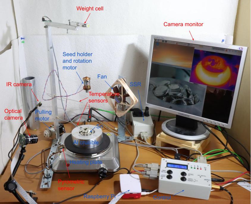
Figure 1: Setup for CZ model experiments: photograph incl. control unit and sensors.

Vertical motion of the seed holder is realized with a stepper motor and a 1:5.18 planet gear box. A thread wheel with a diameter of 30 mm enables vertical velocities up to about 10 mm/s. However, continuous motion is limited by the minimum motor step of 1.8°, which translates to a vertical length of 0.1 mm. Seed rotation by a small DC motor including a miniature gear box is possible in the range 0.5…20 rpm. A fan with a diameter of 120 mm and variable rotation speed in the range 300…1200 rpm is applied for the cooling of the crystal.

The measurement system consists of the following components:

• Type K thermocouples immersed into the melt and approximately 10 cm above the crucible;

• PT100 temperature sensors inserted in a crucible hole and apart from the setup measuring ambient air temperature;

• Pyrometric sensor aimed on a sticker with known emissivity (0.95) on the crucible side;

• Load cell measuring the weight on the pulling wire with a maximum load of 1 kg and resolution of 0.1 g;

• Current sensor to determine the power consumed by the hotplate;

• Longwave (8–14 µm) infrared camera to observe the temperature distribution on the surfaces of hotplate, crucible, and crystal;

• Visible light camera to observe the growth processes and the meniscus in particular.

The hotplate and its temperature stability has a crucial role for the growth process. While there are many lab hotplates available with already integrated temperature control, it turned out that they can produce temperature oscillations up to 10 K (see App. A). Therefore, a common household hotplate with a resistive heater (power rating of 1500 W) was combined with a PID controller running on an Arduino microcontroller. An on/off mode with a period of 20 s, and on-time in the range 2…10 s was implemented for the relay. Stability of crucible temperature of 1 K was achieved up to about 350 °C. Higher stability would probably require control of supplied power using a thyristor.

All hardware components are controlled by an Arduino microcontroller and Raspberry Pi microcomputer, see App. A for further details. The setup described in this section is being published with open hardware and open source software. The cost of the experimental setup does not exceed 1,000 €, where approximately a half was needed for sensors. Therefore, this simple CZ setup could be used also for various demonstration and educational purposes.

3 Growth experiment

In this section, a CZ growth experiment with tin (Sn) is described. Tin pellets of 99.9% purity were used as raw material for the growth experiment. A seed was cut out of a thin Sn crystal with 1.3 mm diameter from a previous pulling experiment with a high pull speed. A filled crucible as shown in Fig. 1 was heated following temperature ramps and arriving at 234 °C with molten tin after 60 min (see Fig. 2). After mechanically removing the oxide layer from the melt surface, the seed was lowered from its initial position 100 mm above the crucible and dipped into the melt. The growth process started with a pull speed of 2 mm/min for the first 20 min, followed by 4 mm/min for 10 min and 6 mm/min for the last 40 min. Crucible temperature was increased from 234 °C at growth start to 240 °C within 50 min. The cooling fan was running at 600 rpm, from the end of melting. The entire process was running automatically according to a predefined recipe, see App. A for further details. This recipe allowed to obtain a crystal with an approximately constant diameter of 10…13 mm as shown in Fig. 2. With constant pull rate and crucible temperature, crystal diameter increased over length, it was significantly smaller without the cooling fan. The cross-section of the crystal was lens-shaped, which is probably caused by crystallographic orientation of an (at least) partly single crystal and by thermal melt inhomogeneities. Crystal rotation generally enhanced round sections in other experiments. A more detailed study including crystal characterization is planned later.

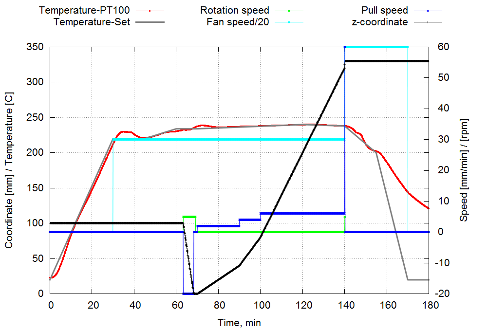
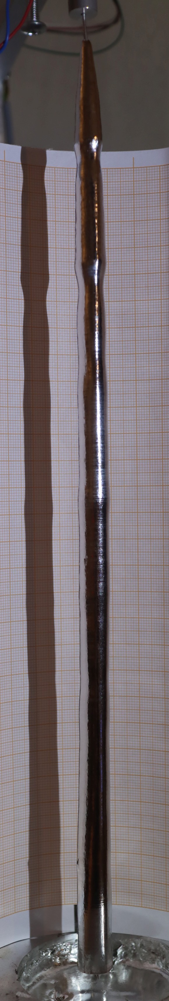
Figure 2: Plot of the process data (left) and photo of the grown Sn crystal (diameter 10…13 mm) with a shadow on a scale paper (right).

Other sensor measurements in addition to crucible temperature are summarized in Fig. 3. Melt temperature was measured about 1 K higher than crucible temperature, a larger deviation occurs after 120 min when the thermocouple becomes only partly covered by the melt. Air above the crucible reaches 50 °C, with flow-induced oscillations in an interval of about 5 °C, while the ambient temperature stays at 22.5±0.3 °C. The pyrometric measurement of crucible temperature using an emissivity sticker was not successful due to sensor malfunction not applying the correct emissivity. The infrared camera image shows a realistic temperature distribution on the hot plate (with emissivity close to 1.0) indicating that it does not exceed much the temperature of the crucible at the emissivity sticker. The metallic surfaces of tin and aluminum do not allow one to detect the temperature in the infrared image because of the low surface emissivity and reflections. Such measurements would work better, e.g., with a crucible made of graphite and an oxide as a model material.

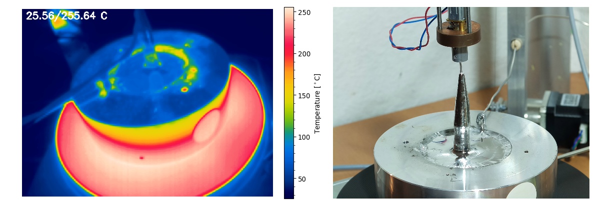
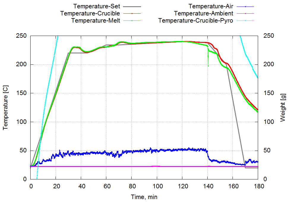
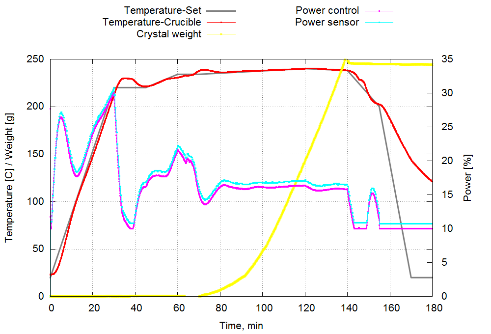
Figure 3: Further in-situ measurements: IR & optical image (top) and various sensor data (bottom).

The discrepancy between the setpoint and actual temperature in Fig. 3 allows one to understand the plot of power control. The power percentage is evaluated from the on-time divided by the 20 s period, so that the 16% power level during the growth phase corresponds to 3.2 s on-time and 16.8 s off-time and an average heating power of 240 W (16% of 1500 W). Note that the minimum on-time was set to 2 s, so that 10% corresponds to zero heating (e.g., after 155 min in Fig. 3, when the actual cooling is slower than the specified ramp). The power data extracted from the current sensor shows slightly higher values than applied in the power control in Fig. 3. This is related to the time constant of the active rectifier and peak detection for the current signal consisting of packets of 50 Hz sinusoidal waves.

Finally, data from the crystal weight sensor is given in Fig. 3. All relevant phases of the growth process can be identified: dipping in the seed at 63 min, where the weight shortly becomes negative; growth start at 70 min, where the weight sharply increases; non-linear increase during the cone growth up to about 90 min; approximately linear increase in the remaining part, where the crystal grows with an approximately constant diameter. A weight of 255 g is reached at the end of the process, while the dismounted crystal showed only 216 g on a laboratory scale. When the crystal was re-attached to the seed mount, a weight of 241 g was measured. This discrepancy of 12% can be explained by the previous calibration of the weight sensor with calibrated weights put on the top of the cell (see Fig. 1). A later test with hanging weights in the range 100…500 g confirmed that the present geometry of the weight cell, metallic thread, and guiding pulleys lead to an apparent weight increase by 12%. The further increase by 6% at the end of the growth process could be related to the friction at the metallic thread. It should be noted that a weight cell with an appropriate operating temperature specification should be used, otherwise deviations as high as 1 g/°C with changing weight cell temperature above the hot plate may occur.

4 Analytical estimations

The goal of this section is to develop a basic physical picture of the growth experiment described above. The focus lays on macroscopic physical phenomena such as heat transfer, electromagnetism, fluid flows, and solid stresses. The following paragraphs present analytical expressions for these phenomena and discuss the relevance of various effects in the growth process. Although a specific CZ growth setup is discussed, most of the estimations can be easily applied to different growth methods and are summarized in Appendix B. The developed simple physical pictures will be compared to results from numerical models in the next section. Material properties of tin are given in Tab. 1 and are compared (for latter reference) to elemental semiconductors silicon (Si) and germanium (Ge).

Property		Units	Si(S)	Ge(S)	Sn(S)	Si(L)	Ge(L)	Sn(L)
Density	$\rho$	kg/m3	2330	5370	7280	2560	5534	6980
Heat capacity	$c$	J/kgK	1040	418	257	1004	358	257
Thermal conductivity	$\lambda$	W/mK	23	17	60	62	48	32
Melting point	$T_{0}$	°C	1412	937	232	–	–	–
Latent heat	$q_{0}$	J/kg	1.8·106	4.6·105	6.1·104	–	–	–
Emissivity	$\epsilon$	–	0.46	0.55	0.07	0.2	0.2	0.1
Thermal expansion coef.	$\beta$	1/K	4.5·10-6	7.5·10-6	2.2·10-5	1·10-4	1·10-4	1·10-4
Viscosity	$\eta$	Pa·s	–	–	–	5.7·10-4	6.8·10-4	0.002
Surface tension	$\gamma$	N/m	–	–	–	0.83	0.6	0.56
Young’s modulus	$E$	GPa	144	118	50	–	–	–
Shear modulus	$G$	GPa	59	50	18	–	–	–
Electrical conductivity	$\sigma$	S/m	3.2·104	1·105	4·106	1.4·106	1.4·106	1.2·106

Table 1: Physical properties of Ge and Si compared to Sn, in liquid (L) and solid (S) (close to melting point) states.

The first model addresses the heat balance in the crystal (see, e.g. [BS11]) during the growth considering a crystal height of $H=100\textrm{~{}mm}$ and a diameter of $D=10\textrm{~{}mm}$. Heat flows into the crystal at the crystallization interface (area $S_{0}=\pi D^{2}/4$) due to the latent heat $Q_{lat}=S_{0}\rho_{S}q_{0}v$ and temperature gradient in the melt $Q_{melt}=S_{0}\lambda_{L}\frac{T_{m}-T_{0}}{h}$. Assuming a melt temperature of $T_{m}=237\textrm{~{}\textdegree C}$ (see Fig. 3) and height $h=10\textrm{~{}mm}$ we obtain $Q_{cond}=1.3\textrm{~{}W}$. The latent heat results in $Q_{lat}=2.3\textrm{~{}W}$ for a growth velocity of $v=4\textrm{~{}mm/min}$. Heat flows out of the crystal at the side surface (area $S_{S}=\pi DH$) due to radiation $Q_{rad}=S_{S}\epsilon_{S}\sigma_{sb}(T_{S}^{4}-T_{a}^{4})$ and gas convection $Q_{conv}=S_{S}\alpha(T_{s}-T_{a})$, where $T_{a}=23\textrm{~{}\textdegree C}$ is the ambient temperature. The crystal surface temperature is obviously somewhere in the range $T_{0}=232\textrm{~{}\textdegree C}$…$T_{a}=23\textrm{~{}\textdegree C}$, so that we obtain $Q_{rad}\leq\textrm{0.7~{}W}$. Due to heat balance $Q_{melt}+Q_{lat}=\textrm{3.6~{}W}=Q_{conv}+Q_{rad}$ we can further estimate $Q_{conv}=\textrm{2.9\ldots 3.6~{}W}$ and $\alpha=\textrm{4.6~{}W/m\textsuperscript{2}K}$ for $T_{S}=T_{0}$. Consequently, heat loss by air convection seems to dominate. Note that heat loss through conduction in the seed was neglected due to the small seed diameter and punctual contacts to the mount.

Electromagnetic phenomena in crystal growth are often related to the induction of heat and forces in the melt (see, e.g. [LFA15, Dad12]). In the present setup, heat is generated in a resistance heater within the hot plate, which is supplied with 50 Hz AC current. The current $I$, voltage $U$, and power $P$ are related by $P=I^{2}_{\mathrm{eff}}R$ and $U_{\mathrm{eff}}=I_{\mathrm{eff}}R$. From $P=1500\textrm{~{}W}$ and $U_{\mathrm{eff}}=230\textrm{~{}V}$ we obtain $I_{\mathrm{eff}}=6.6\textrm{~{}A}$ and $R=35\,\Omega$. Measurements with the current sensor showed a current amplitude of 9 A, corresponding to an effective value of 6.4 A. As a theoretical exercise let us consider possible induction effects from the current with frequency $f=50\textrm{~{}Hz}$. The skin depth in liquid tin can be estimated as $\delta_{em}=1/\sqrt{\mu_{0}\pi f\sigma}=65\textrm{~{}mm}$. The magnetic field is estimated assuming a circular current with diameter $D=120\textrm{mm}$: $B=\mu_{0}I/D=0.1\textrm{~{}mT}$. A first estimation (assuming expressions for a distinct skin effect) of the induced heat $Q_{em}=B_{0}^{2}/2\mu_{0}^{2}\sigma\delta_{em}=0.04~{}\textrm{W/m\textsuperscript{2}}$ (or 0.6 Wm³ if divided by skin depth) and induced force $F_{em}=B_{0}^{2}/2\mu_{0}\delta_{em}=0.06\textrm{~{}N/m\textsuperscript{3}}$ present practically negligible values.

Due to the temperature gradients, buoyant convection (see, e.g. [BS11]) takes place both in the melt and in the surrounding air. The buoyancy forces $F_{buoy}=\rho g\beta\Delta T$ can be estimated to 34 N/m³ and 3 N/m³ assuming temperature differences of 5 °C and 100 °C in the melt and air ($\rho=\textrm{1~{}kg/m\textsuperscript{3}}$, $\beta=\textrm{0.003~{}1/K}$, $\eta=2\cdot 10^{-5}\textrm{~{}Pa s}$, $c=1000~{}\textrm{J/kg K}$, $\lambda=0.03\textrm{~{}W/mK}$), respectively. To obtain a characteristic flow velocity, it is assumed that this force accelerates a fluid volume for a length $L$ as $u=\sqrt{2LF/\rho}$.This leads to 0.01 m/s for the melt ($L=10\textrm{~{}mm}$) and 0.8 m/s for air ($L=100\textrm{~{}mm}$).

The free melt surface and the meniscus at the crystal (see, e.g. [Duf10]) have a central role in the growth process. Meniscus height can be approximated with $h_{m}=a\sqrt{1-sin\beta_{0}}$, where $a=\sqrt{2\gamma/\rho g}=4\textrm{~{}mm}$ and $\beta_{0}$ is the angle between the vertical direction and the meniscus. Obviously, if the solid/liquid contact angle is approximately zero, crystal diameter increases with $\beta_{0}>0$, decreases with $\beta_{0}<0$, and remains constant with $\beta_{0}=0$. On the other hand, meniscus height is determined by the position of the triple line (i.e., outer edge of the crystallization interface). Consequently, an upward moving crystallization interface means an increasing meniscus height $h_{m}$, a decreasing meniscus angle $\beta_{0}$, leading to decreasing crystal diameter, and vice versa. Motion of the crystallization interface occurs if the thermal balance $Q_{melt}+Q_{lat}=Q_{conv}+Q_{rad}$ is not fulfilled, so that thermal conditions are related to dynamic changes in crystal diameter.

Finally, the heat flow through the crystal and the related temperature gradients cause thermal stresses (see, e.g. [TG70]). A simple estimation of the stress level can be based on Hooke’s law: $\sigma_{T}=E\beta\Delta_{r}T$. However, the radial temperature difference in the crystal must be applied. From the previous thermal model we obtain $\Delta_{r}T=(Q_{rad}+Q_{conv})\cdot R/S_{s}\lambda=0.1~{}\textrm{~{}K}$, which leads to a thermal stress of 110 kPa.

5 Numerical modeling

The next step after a description and analysis of the physical phenomena involved in the growth process is a quantitative numerical model. In this section, the open source finite element program Elmer [Elm] is applied for a 2D multi-physical model. The level of description stays rather general, and the physical assumptions, required input parameters, and main physical results are discussed without going into mathematical or numerical details (see Elmer Models manual [Råb+23]). This perspective might well be the preferred one for practical crystal growers. Here, it allows one to focus on the topic of validation, i.e., to separate this topic from verification [Dad+17] and other more technical aspects.

The geometry and a triangular mesh are created by Gmsh [Gms] using a GEO script. The geometry includes tin melt and crystal, crucible, hot plate, coil below the plate (for the electromagnetic calculation) and the air domain with 60 cm diameter and 50 cm height. The model in Elmer is defined using a SIF file. The used Elmer modules, applied physical assumptions and the corresponding source terms and boundary conditions are summarized in Tab. 2. Together with geometric simplifications and material properties (see Tab. 1 for Sn(L) and Sn(S)) these are the input data for the model. A discussion follows in the next section, but note that similar approaches as shown in Tab. 2 have been often used in the literature for crystal growth simulation.

Elmer module and main equations	Physical assumptions	Source terms & boundary conditions
HeatSolve: Heat conduction eq.	• Fixed crystallization interface (may be non-isothermal) • Radiation to ambient (not surface to surface)	• Homogeneous heat source in hot plate (adjusted to reach melting temperature at triple point) • Prescribed latent heat on crystallization interface • Radiation to ambient and convective cooling on solid surfaces
MagnetoDynamics-2D: Vector potential eq.	• Ring current • Limited air domain	• Prescribed current density in coil • Zero magnetic potential on outer boundary
FlowSolve: Navier-Stokes eq.	• Laminar melt flow • Incompressible, laminar gas flow • Limited gas domain	• Buoyancy forces in Boussinesq approximation • No-slip condition on ALL surfaces • Increased viscosity: 10x in melt, 100x in air
StressSolve: Navier eqns.	• Rigid seed mount • Isotropic material • Non-isothermal crystallization interface	• Thermal stress in the crystal • Zero displacement on seed/crystal boundary

Table 2: Model settings for a numerical 2D simulation using Elmer.

Selected results from Elmer calculations are shown in Fig. 4. They describe a steady-state where the heating power has been adjusted to obtain the melting temperature at the triple line and the latent heat corresponds to growth with 3 mm/min. The resulting heating power was 104 W, it decreased to 83 W without convective cooling in air and to 75 W with only radiation in air. These powers are smaller than 240 W measured in the experiment. Summary of heat flows on various surfaces in Tab. 3 indicates that heat radiation dominates heat losses from the hotplate with emissivity $\epsilon=0.5$ and has a comparable influence to convection on other surfaces with emissivities $\epsilon\leq 0.1$. The calculated minimum crystal temperature was at least 209°C.

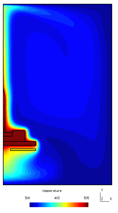
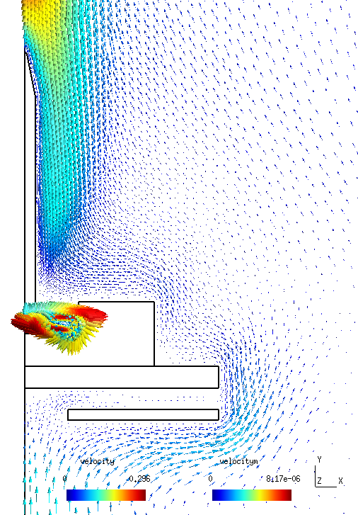
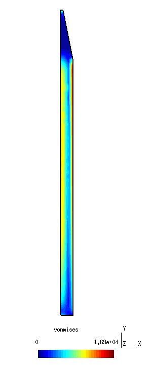
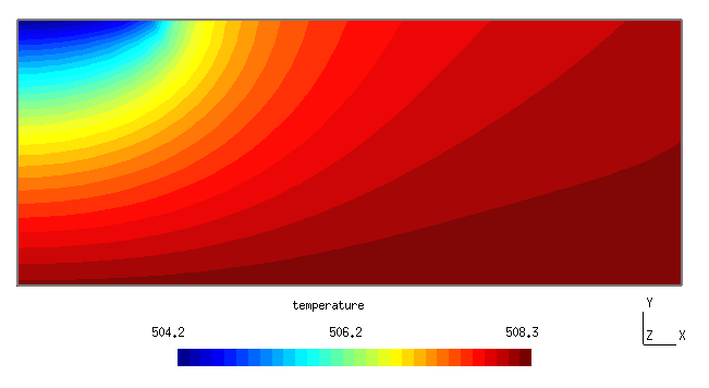
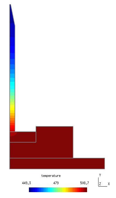
Figure 4: Numerical 2D simulation with Elmer: temperature isolines [K], velocity vectors for melt and gas flows [m/s] , thermal stress [Pa] in the crystal (top); thermal calculation with applied heat transfer coefficients from OpenFOAM (bottom).

The calculation of melt and gas flows in Elmer had convergence issues even in unsteady calculations, and solutions could be obtained only with artificially increased viscosities (improving the numerical stability) of 10x in the melt and 100x in the air. Flow velocity reaches 0.01 mm/s in the melt and 0.3 m/s in the air, where the former value is even 3 orders of magnitude smaller than estimated in Sec. 4. Although the temperature differences in the aluminum crucible are below 1 K, the direction of the resulting gradient at the melt side obviously determines flow direction. A heat flow from the melt into the crucible wall leads to an upward buoyant flow at the melt side. The calculated gas flow pattern consists of an upward buoyant flow along the hot crystal surface as expected.

Comparative 2D calculation for the melt and gas flows were performed using OpenFOAM [Ope]. The triangular mesh of the gas domain was rotated (extruded) in Gmsh to a 5° wedge creating prismatic 3D elements, see Fig. 5. Simplified boundary conditions with constant surface temperatures (gas domain: 494 K at crystal, 505 K at other solids; melt domain: 505 K at crystal, 508 K at crucible bottom, zero heat flux at other boundaries) from Elmer calculation were applied. Unsteady calculations using the incompressible buoyantBoussinesqPimpleFoam solver with upwind schemes for the convective terms typically reached a stationary state before 100 s. The global gas flow pattern and the characteristic velocity shown in Fig. 5 remained similar to Fig. 4, although some recirculation vortices appeared at the melt free surface. However, the convective heat fluxes were much higher than in the previous Elmer calculation. The heat transfer coefficients (HTC) were estimated as $\alpha=3\textrm{~{}W/m\textsuperscript{2}K}$ on melt free surface and $\alpha=6\textrm{~{}W/m\textsuperscript{2}K}$ on other solid surfaces. A thermal calculation with Elmer using these coefficients led to much higher convective heat losses (see Tab. 3 and Fig. 4 (bottom) for resulting temperature fields) and a total heating power of 173 W. Obviously, the artificially increased viscosity may cause underestimated convective heat exchange. The melt flow calculation in OpenFOAM reaches a velocity of 2 mm/s, which is much higher than in Elmer.

Surface	With conv.	No conv.	Rad. only	With HTC
Crystal ($\epsilon=$0.07)	1.7	1.4	0.8 (0.8)	4.3
Melt ($\epsilon=$0.1)	0.7	0.6	0.5 (0.6)	2.2
Crucible ($\epsilon=$0.05)	13.2	6.6	5.0 (3.3)	32.5
Hotplate ($\epsilon=$0.5)	89.5	76.1	70.2 (72)	136.4
Sum	105.1	84.7	76.5	175.4
Heating	103	83	75	173
Crystal min. T	482 K	485 K	496 K	449 K

Table 3: Heat flows in [W] in various calculations with Elmer evaluated using SaveScalars procedure and Diffusive flux operator with 2nd order elements. In the case “Rad. only” analytical estimation is given in brackets ().

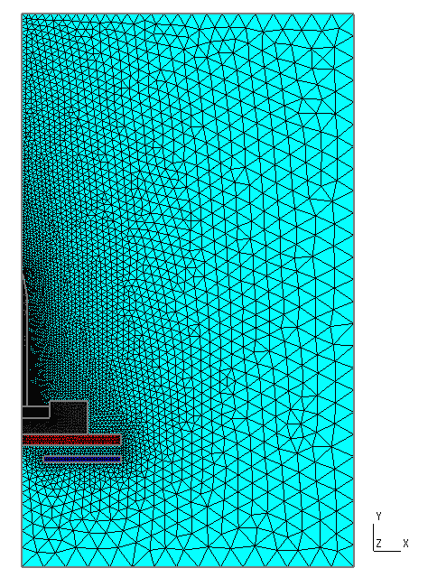
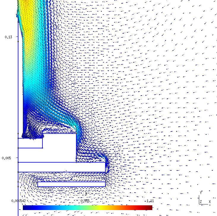
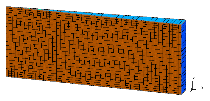
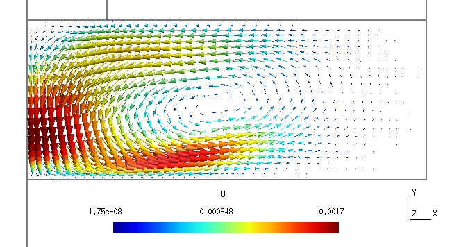
Figure 5: Numerical 2D simulation with OpenFOAM: grid (left), velocity vectors [m/s] for melt and gas flows (right).

The electromagnetic calculation considers an AC current below the hotplate producing a magnetic field, which generates eddy currents in electrically conducting bodies. If a non-conducting crucible material is considered, the liquid tin melt is subject to a magnetic flux density of 0.2 mT, induced heat power up to 0.03 W/m³, and induced Lorentz force densities up to 0.0001 N/m³. Obviously the inductive effects are negligible both for the thermal and melt flow calculation. As a theoretical exercise, another case was calculated for an inductive hotplate with a frequency of 22 kHz and a current of 30 A in 20 windings. A graphite crucible with an electrical conductivity of 5·10⁴ S/m leads to a magnetic flux density of 11 mT, induced heat power up to 2·10⁶ W/m³ in the crucible and 8·10⁵ W/m³ in the melt, induced Lorentz force densities in the melt up to 10³ N/m³. In this case, significant electromagnetic effects can be expected.

Thermal stress in the crystal was calculated assuming isotropic elastic properties. As shown in Fig. 4, the von Mises stress first decreases radially, but then increases and reaches a maximum of 2·10⁴ Pa at the crystal rim. The stress components $\sigma_{ij}$ have radially monotonous distributions with values up to 10⁴ Pa. While the case in Fig. 4 has a rather low stress level at the crystallization interface, artificial local maxima may occur due to local thermal gradients caused by the prescribed flat interface shape.

Note that all simulations described here were done on the Raspberry Pi computer used for process monitoring in Sec. 2. This approach would allow the implementation of advanced algorithms for process control involving both in-situ measurement data and live numerical models. The source code for Elmer and OpenFOAM models is available as open source (see App. A).

6 Discussion

The analytical models in Sec. 4 and numerical models in Sec. 5 both describe a CZ growth process in terms of selected physical pictures. In the following sections, main results from both approaches are discussed and compared to achieve the following goals:

• Develop a physical understanding of the CZ growth process on a macroscopic level.

• Identify open questions in the modeling methods and propose solutions in terms of verification and validation.

The analysis of heat balance in the crystal in Sec. 4 arrived at the conclusion that heat loss due to air convection at the crystal surface exceeds heat radiation several times. While first numerical results in Elmer indicated an opposite relation, a closer analysis of air convection confirmed the dominating influence of convection even if crystal surface temperature drops only about 20 K below the melting point. It can be concluded:

• The effect of convective cooling may be grossly underestimated in simplified models of gas flows with artificially increased viscosities, under-resolved boundary layers, etc. Verification using benchmark cases and validation using measurements of crystal/seed temperatures is recommended.

• Accuracy of integral heat fluxes in numerical models should be verified with analytical solutions. Use of second order elements in Elmer were crucial to obtain accurate results.

In the sense of a global heat balance of the growth setup, the sum of all heat losses should be equal to the heating power (plus a small contribution by the latent heat). The numerically calculated power of 173 W is smaller than the measured power of 240 W by almost 30%. To explain such deviations:

• Heat losses missing in the numerical model could be identified (i.e., validated) in the experimental setup using thermal imaging and additional temperature or heat flux measurements to find theoretically unexpected cold spots.

• Material properties with a large degree of uncertainty and large influence on the heat balance (e.g., emissivity of solid surfaces) should be validated in dedicated experiments, e.g., using pyrometric measurements.

The measurement of the AC heater current allowed us to calculate the heat and force induction in the melt. While the analytical and numerical values of the magnetic field agree well, the induced heat density and force density are smaller by 1–3 orders of magnitude in the numerical simulation for the 50 Hz case. While the induction effects remain negligible both in simulation and estimation, for the application of higher frequencies such as 22 kHz, a closer analysis of such discrepancies is recommended.

• In addition to the heater power, the measurement of the heater current or the related magnetic field is a prerequisite for further analysis of induction effects. This can be seen as validation of heater models for complex heater shapes and temperature- dependent properties.

• The numerical calculation of heat and force induction should be verified using analytical solutions for simple geometries.

Buoyant convection in the air is obviously responsible for the strong effect of convective cooling discussed above. Despite the strongly simplified boundary conditions for the air flow in the numerical models with Elmer and OpenFOAM, the calculated typical velocities agree with the analytical estimation. On the contrary, the numerically calculated velocity for the melt flow is nearly 3 orders of magnitude smaller in Elmer. The following general aspects may be emphasized here:

• Artificial increase of fluid viscosity (as tested in Elmer) to improve the numerical convergence may lead to large deviations in the calculated velocity magnitude and heat transfer coefficients.

• Boundary conditions for gas flows should be validated with velocity or pressure measurements to enable physically meaningful solutions also for strongly simplified models (such as a closed box with cold walls).

• High thermal conductivity of the melt may lead to very low thermal gradients, so that even small changes in local thermal conditions may influence the resulting buoyant flow pattern. Both a validation of the thermal model with accurate temperature measurements and velocity measurements in the melt are recommended.

In the numerical simulation with Elmer, a flat free melt surface with a fixed triple line position was assumed. Consequently, the liquid meniscus at the crystal was neglected. Analytical estimation leads to a meniscus height of 4 mm for a meniscus angle of 0°. The understanding of the dynamic changes of crystal diameter and development of related analytical or numerical models would be hardly possible without considering the following aspects:

• A validation using optical observation of the triple line region is crucial. The exact relationship between growth angle and meniscus height may be not only material-dependent but also process dependent.

• A fixed triple line and neglected undercooling in the simulation may lead to unphysical results such as artificial thermal gradients. Such assumptions should be validated with measurements of temperature and crystallization interface shape.

Thermal stress in the crystal is a direct consequence of the temperature non-linearity and the mechanical constraints. The analytical estimation arrived at about 100 kPa and the numerical calculation at 10 kPa, the latter with a relatively constant radial profile over a large part of the crystal height. This can be probably explained with the trivial analytical formula. Nevertheless, some assumptions in numerical models may need a closer attention:

• The thermal model of the crystallization interface (e.g., deviations from an isotherm) may cause artificial local stresses. This model should be verified with analytical or accurate numerical solutions.

• The non-linearity of the temperature distribution may be enhanced by local thermal asymmetries, small deviations from the idealized crystal shape and other hardly measurable factors. Here a validation using a dummy crystal allowing for in-situ stress analysis in a comparable thermal process could be helpful.

Although the discussed aspects above mostly arose from the analysis of a very specific CZ growth process, a wider literature study about modeling of CZ growth demonstrated similar open questions in model validation [EPD22]. Furthermore, one might expect similar issues in many other growth processes (and comparable multi-physical processes) sharing the same basic physical phenomena. This conclusion has served as a motivation for the NEMOCRYS project [Nex], where the following strategy is being applied:

1. Identify open questions in models of crystal growth processes.

2. Develop model experiments with extensive in-situ measurements.

3. Build new validated coupled models for crystal growth.

This study presented a simple model experiment for CZ growth, basic techniques for in-situ measurements, and simplified numerical models based mainly on theoretical considerations. The next iteration with respect to CZ model setups and in-situ measurements [EPD22] as well as validated numerical models [EPD22a] has already been published. It is also planned to extend this approach to other crystal growth methods such as the floating zone process with inductive and/or optical heating.

Finally, it should be noted that Sn has been already used as a model material for CZ growth in the literature [EC86]. Tab. 1 compares material properties relevant for a macroscopic analysis of the growth process between Sn and elemental semiconductors Si and Ge, where the CZ growth has a great practical significance. It can be seen that some properties agree relatively well, while others such as the latent heat differ more than by an order of magnitude. A more exact analysis of the physical similarity between the present experiment with Sn and CZ growth of Si or Ge on small or large scales would be possible using analytical estimates (as in Sec. 4) and dimensionless numbers [Dad12, DPG20].

7 Conclusions and outlook

A new low-cost experimental setup with open hardware and open source software has been developed for the CZ crystal growth process of model materials up to about 350 °C. The compact size of the setup, its automation capabilities as well as detailed in-situ measurements enable the application of this setup not only for demonstration and educational purposes but also for small-scale conceptual studies.

In the present study, tin crystals with diameters of about 12 mm and lengths up to 320 mm were grown. In contrast to the historic experiments by Jan Czochralski in 1916, the main focus was not on the determination of the highest achievable growth rates but rather on a reproducible growth process with comprehensive in-situ observation to extract the typical physical phenomena of CZ growth in the sense of a model experiment.

The analysis of the experiment allowed to set up analytical and numerical models describing the physical aspects of heat transfer, electromagnetism, melt and gas flows as well as solid stresses in CZ growth. The following discussion of the theoretical and experimental data demonstrated a new strategy for the development and validation of macroscopic crystal growth models.

Following the proposed strategy, new model experiments will be developed for various crystal growth processes in the NEMOCRYS project. They will be applied to address the many open questions in crystal growth simulation and in the complex interaction of various physical phenomena. In summary, Jan Czochralski’s experiment in its simplicity teaches us to separate the core scientific principle of the CZ method from the following technological advances. It is helpful to look for deep answers to simple (modeling) questions before trying simplified answers to deep (modeling) questions.

Appendix A Online materials (in preparation)

Schematics and tests of the Arduino-based control: https://github.com/nemocrys/czdemo-exp

Source code for the Arduino-based control: https://github.com/nemocrys/czdemo-exp/tree/master/arduino

Python scripts for visualization of camera images and measurement data as well as for preparing and uploading growth recipes on the Raspberry Pi: https://github.com/nemocrys/czdemo-exp/tree/master/raspberrypi

Interactive simulation of the Czochralski growth proces in Python: https://github.com/nemocrys/crystal-game

Source code for the solvers in Elmer and OpenFOAM: https://github.com/nemocrys/czdemo-sim

Appendix B Analytical estimation of crystal growth processes

References

- [Ant20] Olli Anttila “Czochralski growth of silicon crystals” 00006 ZSCC: 0000006 In Handbook of Silicon Based MEMS Materials and Technologies Elsevier, 2020, pp. 19–60 DOI: 10.1016/B978-0-12-817786-0.00002-5
- [BS11] Hans Dieter Baehr and Karl Stephan “Heat and Mass Transfer” Springer, 2011 DOI: 10.1007/978-3-642-20021-2
- [Czo18] J. Czochralski “Ein neues Verfahren zur Messung der Kristallisationsgeschwindigkeit der Metalle” ZSCC: 0000848 In Zeitschrift für Physikalische Chemie 92U.1, 1918, pp. 219–221 DOI: 10.1515/zpch-1918-9212
- [Dad+16] K. Dadzis et al. “Directional melting and solidification of gallium in a traveling magnetic field as a model experiment for silicon processes” ZSCC: 0000020 tex.ids: dadzisDirectionalMeltingSolidification2016a In Journal of Crystal Growth 445, 2016, pp. 90–100 DOI: 10.1016/j.jcrysgro.2016.03.037
- [Dad+17] K. Dadzis, P. Bönisch, L. Sylla and T. Richter “Validation, verification, and benchmarking of crystal growth simulations” ZSCC: 0000005 tex.ids: dadzisValidationVerificationBenchmarking2017a publisher: Elsevier BV In Journal of Crystal Growth 474, 2017, pp. 171–177 DOI: 10.1016/j.jcrysgro.2016.12.091
- [Dad12] Kaspars Dadzis “Modeling of directional solidification of multicrystalline silicon in a traveling magnetic field” ZSCC: NoCitationData[s0], 2012 URL: https://nbn-resolving.org/urn:nbn:de:bsz:105-qucosa-117492
- [Der10] Jeffrey J. Derby “Modeling and bulk crystal growth processes: What is to be learned?” In AIP Conference Proceedings 1270, 2010, pp. 221–244 DOI: 10.1063/1.3476228
- [DPG20] Kaspars Dadzis, Olf Pätzold and Gunter Gerbeth “Model Experiments for Flow Phenomena in Crystal Growth” ZSCC: 0000001 tex.ids= dadzisModelExperimentsFlow2019, dadzisModelExperimentsFlow2020 number: 2 publisher: Wiley In Crystal Research and Technology 55.2, 2020, pp. 1900096 DOI: 10.1002/crat.201900096
- [Duf10] “Crystal Growth Processes Based on Capillarity: Czochralski, Floating Zone, Shaping and Crucible Techniques” Wiley, 2010
- [EC86] Urban Ekhult and Torbjörn Carlberg “Czochralski growth of tin crystals under constant pull rate and IR diameter control” ZSCC: 0000018 In Journal of Crystal Growth 76.2, 1986, pp. 317–322 DOI: 10.1016/0022-0248(86)90377-5
- [Elm] “Elmer FEM: open source multiphysical simulation software” Elm URL: http://www.elmerfem.org
- [EPD22] A. Enders-Seidlitz, J. Pal and K. Dadzis “Development and validation of a thermal simulation for the Czochralski crystal growth process using model experiments” In Journal of Crystal Growth 593, 2022, pp. 126750 DOI: 10.1016/j.jcrysgro.2022.126750
- [EPD22a] A. Enders-Seidlitz, J. Pal and K. Dadzis “Model experiments for Czochralski crystal growth processes using inductive and resistive heating” 1 citations (Crossref) [2022-11-29] ZSCC: 0000000 ZSCC: NoCitationData[s0] Publisher: IOP Publishing In IOP Conference Series: Materials Science and Engineering 1223.1, 2022, pp. 012003 DOI: 10.1088/1757-899X/1223/1/012003
- [Gms] “Gmsh: A three-dimensional finite element mesh generator with built-in pre- and post-processing facilities” Gms URL: https://gmsh.info/
- [LFA15] Sergio Lupi, Michele Forzan and Aleksandr Aliferov “Induction and Direct Resistance Heating” Springer, 2015 DOI: 10.1007/978-3-319-03479-9
- [Nex] “Next Generation Multiphysical Models for Crystal Growth Processes” Nex URL: https://cordis.europa.eu/project/id/851768
- [Ope] “OpenFOAM is the free, open source CFD software” Ope URL: https://www.openfoam.com/
- [Råb+23] Peter Råback et al. “Elmer Models Manual”, 2023 URL: https://www.elmerfem.org/blog/documentation/
- [TG70] S.. Timoshenko and J.. Goodier “Theory of elasticity” McGraw-Hill Book Company, 1970
- [Uec14] Reinhard Uecker “The historical development of the Czochralski method” ZSCC: 0000035 In Journal of Crystal Growth 401, 2014, pp. 7–24 DOI: 10.1016/j.jcrysgro.2013.11.095