[caption,subcaption]

Liu, Grigas, Liu, and Shen Active Learning in the Predict-then-Optimize Framework: A Margin-Based Approach

Active Learning in the Predict-then-Optimize Framework: A Margin-Based Approach

Mo Liu Department of Industrial Engineering and Operations Research, University of California, Berkeley, Berkeley, CA, 94720, mo_liu@berkeley.edu Paul Grigas Department of Industrial Engineering and Operations Research, University of California, Berkeley, Berkeley, CA, 94720, pgrigas@berkeley.edu Heyuan Liu Department of Industrial Engineering and Operations Research, University of California, Berkeley, Berkeley, CA, 94720, heyuan_liu@berkeley.edu Zuo-Jun Max Shen Department of Industrial Engineering and Operations Research, University of California, Berkeley, Berkeley, CA, 94720, maxshen@berkeley.edu

We develop the first active learning method in the predict-then-optimize framework. Specifically, we develop a learning method that sequentially decides whether to request the “labels” of feature samples from an unlabeled data stream, where the labels correspond to the parameters of an optimization model for decision-making. Our active learning method is the first to be directly informed by the decision error induced by the predicted parameters, which is referred to as the Smart Predict-then-Optimize (SPO) loss. Motivated by the structure of the SPO loss, our algorithm adopts a margin-based criterion utilizing the concept of distance to degeneracy and minimizes a tractable surrogate of the SPO loss on the collected data. In particular, we develop an efficient active learning algorithm with both hard and soft rejection variants, each with theoretical excess risk (i.e., generalization) guarantees. We further derive bounds on the label complexity, which refers to the number of samples whose labels are acquired to achieve a desired small level of SPO risk. Under some natural low-noise conditions, we show that these bounds can be better than the naive supervised learning approach that labels all samples. Furthermore, when using the SPO+ loss function, a specialized surrogate of the SPO loss, we derive a significantly smaller label complexity under separability conditions. We also present numerical evidence showing the practical value of our proposed algorithms in the settings of personalized pricing and the shortest path problem.

active learning, predict-then-optimize, prescriptive analytics, data-driven optimization

1 Introduction

In many applications of operations research, decisions are made by solving optimization problems that involve some unknown parameters. Typically, machine learning tools are used to predict these unknown parameters, and then an optimization model is used to generate the decisions based on the predictions. For example, in the shortest path problem, we need to predict the cost of each edge in the network and then find the optimal path to route users. Another example is the personalized pricing problem, where we need to predict the purchase probability of a given customer at each possible price and then decide the optimal price. In this predict-then-optimize paradigm, when generating the prediction models, it is natural to consider the final decision error as a loss function to measure the quality of a model instead of standard notions of prediction error. The loss function that directly considers the cost of the decisions induced by the predicted parameters, in contrast to the prediction error of the parameters, is called the Smart Predict-then-Optimize (SPO) loss as proposed by Elmachtoub and Grigas (2022). Naturally, prediction models designed based on the SPO loss have the potential to achieve a lower cost with respect to the ultimate decision error.

In general, for a given feature vector $x$, calculating the SPO loss requires knowing the correct (in hindsight) optimal decision associated with the unknown parameters. However, a full observation of these parameters, also known as a label associated with $x$, is not always available. For example, we may not observe the cost of all edges in the graph in the shortest path problem. In practice, acquiring the label of one feature vector instance could be costly, and thus acquiring the labels of all feature vectors in a given dataset would be prohibitively expensive and time-consuming. In such settings, it is essential to actively select the samples for which label acquisition is worthwhile.

Algorithms that make decisions about label acquisition lie in the area of active learning. The goal of active learning is to learn a good predictor while requesting a small number of labels of the samples, whereby the labels are requested actively and sequentially from unlabeled samples. Intuitively, if we are very confident about the label of an unlabeled sample based on our current predictor, then we do not have to request the label of it. Active learning is most applicable when the cost of acquiring labels is very expensive. Traditionally in active learning, the selection rules for deciding which samples to acquire labels for are based on measures of prediction error that ignore the cost of the decisions in the downstream optimization problem. Considering the SPO loss in active learning can hopefully reduce the number of labels required while achieving the same cost of decisions, compared to standard active learning methods that only consider measures of prediction error.

Considering active learning in the predict-then-optimize framework can bridge the gap between active learning and operational decisions, but there are two major challenges when designing algorithms to select samples. One is the computational issue due to the non-convexity and non-Lipschitzness of the SPO loss. When one is concerned with minimizing the SPO loss, existing active learning algorithms are computationally intractable. For example, the general importance weighted active learning (IWAL) algorithm proposed by Beygelzimer et al. (2009) is impractical to implement, since calculating the “weights” of samples requires a large enumeration of all pairs of predictors. Other active learning algorithms that are designed for the classification problem cannot be extended to minimize the SPO loss directly. Another challenge is to derive bounds for the label complexity of the algorithms and to demonstrate the advantages over supervised learning. Label complexity refers to the number of labels that must be acquired to ensure that the risk of predictor is not greater than a desired threshold. To demonstrate the savings from active learning, label complexity should be smaller than the sample complexity of supervised learning, when achieving the same risk level with respect to the loss function of interest (in our case SPO). Kääriäinen (2006) shows that, without additional assumptions on the distributions of features and noise, active learning algorithms have the same label complexity as supervised learning. Thus, deriving smaller label complexity for an active learning algorithm under some natural conditions on the noise and feature distributions is a critical but nontrivial challenge.

In this paper, we develop the first active learning method in the predict-then-optimize framework. We consider the standard setting of a downstream linear optimization problem where the parameters/label correspond to an unknown cost vector that is potentially related to some feature information. Our proposed algorithm, inspired by margin-based algorithms in active learning, uses a measure of “confidence” associated with the cost vector prediction of the current model to decide whether or not to acquire a label for a given feature. Specifically, the label acquisition decision is based on the notion of distance to degeneracy introduced by El Balghiti et al. (2022), which precisely measures the distance from the prediction of the current model to the set of cost vectors that have multiple optimal solutions. Intuitively, the further away the prediction is from degeneracy, the more confident we are that the associated decision is actually optimal. Our proposed margin-based active learning (MBAL-SPO) algorithm has two versions depending on the precise rejection criterion: soft rejection and hard rejection. Hard rejection generally has a smaller label complexity, whereas soft rejection is computationally easier. In any case, when building prediction models based on the actively selected training set, our algorithm will minimize a generic surrogate of the SPO loss over a given hypothesis class. For each version, we demonstrate theoretical guarantees by providing non-asymptotic excess surrogate risk bounds, as well as excess SPO risk bounds, that hold under a natural consistency assumption.

To analyze the label complexity of our proposed algorithm, we define the near-degeneracy function, which characterizes the distribution of optimal predictions near the regions of degeneracy. Based on this definition, we derive upper bounds on the label complexity. We consider a natural low-noise condition, which intuitively says that the distribution of features for a given problem is far enough from degeneracy. Indeed, for most practical problems, the data are expected to be somewhat bounded away from degeneracy. Under these conditions, we show that the label complexity bounds are smaller than those of the standard supervised learning approach. In addition to the results for a general surrogate loss, we also demonstrate improved label complexity results for the SPO+ surrogate loss, proposed by Elmachtoub and Grigas (2022) to account for the downstream problem, when the distribution satisfies a separability condition. We also conduct some numerical experiments on instances of shortest path problems and personalized pricing problems, demonstrating the practical value of our proposed algorithm above the standard supervised learning approach. Our contributions are summarized below.

• We are the first work to consider active learning algorithms in the predict-then-optimize framework. To efficiently acquire labels to train a machine learning model to minimize the decision cost (SPO loss), we propose a margin-based active learning algorithm that utilizes a surrogate loss function.

• We analyze the label complexity and derive non-asymptotic surrogate and SPO risk bounds for our algorithm, under both soft-rejection and hard-rejection settings. Our analysis applies even when the hypothesis class is misspecified, and we demonstrate that our algorithms can still achieve a smaller label complexity than supervised learning. In particular, under some natural consistency assumptions, we develop the following guarantees.

  • In the hard rejection case with general surrogate loss functions, we provide generic bounds on the label complexity and the non-asymptotic surrogate and SPO risks in Theorem 4.5.

  • In the hard rejection case with the SPO+ surrogate loss, we provide a much smaller non-asymptotic surrogate (and, correspondingly, SPO) risk bound in Theorem 4.11 under a separability condition. This demonstrates the advantage of the SPO+ surrogate loss over general surrogate losses.

  • In the soft rejection case with a general surrogate loss, which is computationally easier, we provide generic bounds on the label complexity and the non-asymptotic surrogate and SPO risks in Theorem 4.13.

  • For each case above, we characterize sufficient conditions for which we can specialize the above generic guarantees and demonstrate that the margin-based algorithm achieves sublinear or even finite label complexity. We provide concrete examples of these conditions, and we provide different non-asymptotic bounds in cases where the feasible region of the downstream optimization problem is either a polyhedron or a strongly convex region. In these situations, and under natural low-noise conditions, we demonstrate that our algorithm can achieve much smaller label complexity than the sample complexity of supervised learning.

• We demonstrate the practical value of our algorithm by conducting comprehensive numerical experiments in two settings. One is the personalized pricing problem, and the other is the shortest path problem. Both sets of experiments show that our algorithm achieves a smaller SPO risk than the standard supervised learning algorithm given the same number of acquired labels.

1.1 Example: Personalized Pricing Problem

To further illustrate and motivate the integration of active learning into the predict-then-optimize setting, we present the following personalized pricing problem as an example.

Example 1.1 (Personalized pricing via customer surveys)

Suppose that a retailer needs to decide the prices of $\mathfrak{J}$ items for each customer, after observing the features (personalized information) of the customers. The feature vector of a generic customer is $x$, and the purchase probability of that customer for item $j$ is $d_{j}(p^{j})$, which is a function of the price $p^{j}$. This purchase probability $d_{j}(p^{j})$ is unknown and corrupted with some noise for each customer. Suppose the price for each item is selected from a candidate list $\{p_{1},p_{2},...,p_{\mathcal{I}}\}$, which is sorted in ascending order. Then, the pricing problem can be formulated as

(1)

Here, $\mathbf{w}$ encodes the decision variables with indices in the set $\mathcal{I}\times\mathfrak{J}$, where $w_{i,j}$ is a binary variable indicating which price for item $j$ is selected. Namely, $w_{i,j}=1$ if item $j$ is priced at $p_{i}$, and otherwise $w_{i,j}=0$. The objective (1) is to maximize the expected total revenue of $\mathfrak{J}$ items by offering price $p_{i}$ for item $j$. Constraints (LABEL:con:1price) require each item to have one price selected. In constraint (LABEL:con:sum1), $\mathbf{A}$ is a matrix with $\mathfrak{K}$ rows, and $b$ is a vector with $\mathfrak{K}$ dimensions. Each row of constraints (LABEL:con:sum1) characterizes one rule for setting prices. For example, if the first row of $\mathbf{A}\mathbf{w}$ is $w_{i,j}-\sum_{i^{\prime}=i}^{\mathcal{I}}w_{i^{\prime},j+1}$ and the first entry in $b$ is zero, then this constraint further requires that if item $j$ is priced at $p_{i}$, then the price for the item $j+1$ must be no smaller than $p_{i}$. For another example, if the second row of $\mathbf{A}\mathbf{w}$ is $\sum_{i^{\prime}=1}^{i-1}\sum_{j=1}^{\mathfrak{J}}w_{i^{\prime},j}$, and the second entry of $b$ is 1, then it means that at most one item can be priced below the price $p_{i}$. Thus, constraints (LABEL:con:sum1) can characterize different rules for setting prices for $\mathfrak{J}$ items.

Traditionally, the conditional expectation of revenue $\mathbb{E}[d_{j}(p_{i})p_{i}|x]$ must be estimated from the purchasing behavior of the customers. In this example, we consider the possibility that the retailer can give the customers surveys to investigate their purchase probabilities. By analyzing the results of the surveys, the retailer can infer the purchase probability $d_{j}(p_{i})|x$ for each price point $p_{i}$ and each item $j$ for this customer. Therefore, whenever a survey is conducted, the retailer acquires a noisy estimate of the revenue, denoted by $d_{j}(p_{i})p_{i}|x$, at each price point $p_{i}$ and item $j$.

In personalized pricing, first, the retailer would like to build a prediction model to predict $\mathbb{E}[d_{j}(p_{i})p_{i}|x]$ given the customer’s feature vector $x$. Then, given the prediction model, the retailer solves the problem (1) to obtain the optimal prices. In practice, when evaluating the quality of the prediction results of $d_{j}(p_{i})p_{i}|x$, the retailer cares more about the expected revenue from the optimal prices based on this prediction, rather than the direct prediction error. Therefore, when building the prediction model for $d_{j}(p_{i})p_{i}|x$, retailers are expected to be concerned with minimizing SPO loss, rather than minimizing prediction error.

One property of (1) is that the objective is linear and can be further written as $\max_{\mathbf{w}}\sum_{j=1}^{\mathfrak{J}}\sum_{i=1}^{\mathfrak{K}}\mathbb{E}[d_{j}(p_{i})p_{i}|x]w_{i,j}$. By the linearity of the objective, the revenue loss induced by the prediction errors can be written in the form of the SPO loss considered in Elmachtoub and Grigas (2022). In general, considering the prediction errors when selecting customers may be inefficient, since smaller prediction errors do not always necessarily lead to smaller revenue losses, because of the properties of the SPO loss examined by Elmachtoub and Grigas (2022).

In Example 1.1, in practice, there exists a considerable cost to investigate all customers, for example, the labor cost to collect the answers and incentives given to customers to fill out the surveys. Therefore, the retailer would rather intelligently select a limited subset of customers to investigate. This subset of customers should be ideally selected so that the retailer can build a prediction model with small SPO loss, using a small number of surveys.

Active learning is essential to help retailers select representative customers and reduce the number of surveys. Traditional active learning algorithms would select customers to survey based on model prediction errors, which are different from the final revenue of the retailer. On the contrary, when considering the SPO loss, the final revenue is integrated into the learning and survey distribution processes.

1.2 Literature Review

In this section, we review existing work in active learning and the predict-then-optimize framework. To the best of our knowledge, our work is the first work to bridge these two streams.

Active learning.

There has been substantial prior work in the area of active learning, focusing essentially exclusively on measures of prediction error. Please refer to Settles (2009) for a comprehensive review of many active learning algorithms. Cohn et al. (1994) shows that in the noiseless binary classification problem, active learning can achieve a large improvement in label complexity, compared to supervised learning. It is worth noting that in the general case, Kääriäinen (2006) provides a lower bound of the label complexity which matches supervised learning. Therefore, to demonstrate the advantages of active learning, some further assumptions on the noise and distribution of samples are required. For the agnostic case where the noise is not zero, many algorithms have also been proposed in the past few decades, for example, Hanneke (2007), Dasgupta et al. (2007),Hanneke (2011), Balcan et al. (2009), and Balcan et al. (2007). These papers focus on binary or multiclass classification problems. Balcan et al. (2007) proposed a margin-based active learning algorithm, which is used in the noiseless binary classification problem with a perfect linear separator. Balcan et al. (2007) achieves the label complexity $\mathcal{O}(\epsilon^{-2\alpha}\ln(1/\epsilon))$ under uniform distribution, where $\alpha\in(0,1)$ is a parameter defined for the low noise condition and $\epsilon$ is the desired error rate. Krishnamurthy et al. (2017) and Gao and Saar-Tsechansky (2020) consider cost-sensitive classification problems in active learning, where the misclassification cost depends on the true labels of the sample.

The above active learning algorithms in the classification problem do not extend naturally to real-valued prediction problems. However, the SPO loss is a real-valued function. When considering real-valued loss functions, Castro et al. (2005) prove convergence rates in the regression problem, and Sugiyama and Nakajima (2009) and Cai et al. (2016) also consider squared loss as the loss function. Beygelzimer et al. (2009) propose an importance-weighted algorithm (IWAL) that extends disagreement-based methods to real-valued loss functions. However, it is intractable to directly use the IWAL algorithm in the SPO framework. Specifically, it requires solving a non-convex problem at each iteration, which may have to enumerate all pairs of predictor candidates even when the hypothesis set is finite.

Predict-then-optimize framework.

In recent years, there has been a growing interest in developing machine learning models that incorporate the downstream optimization problem. For example, Bertsimas and Kallus (2020), Kao et al. (2009), Elmachtoub and Grigas (2022), Zhu et al. (2022), Donti et al. (2017) and Ho and Hanasusanto (2019) propose frameworks that somehow relate the learning problem to the downstream optimization problem. In our work, we consider the Smart Predict-then-Optimize (SPO) framework proposed by Elmachtoub and Grigas (2022). Because the SPO loss function is nonconvex and non-Lipschitz, the computational and statistical properties of the SPO loss in the fully supervised learning setting have been studied in several recent works. Elmachtoub and Grigas (2022) provide a surrogate loss function called SPO+ and show the consistency of this loss function. Elmachtoub et al. (2020), Loke et al. (2022), Demirovic et al. (2020), Demirović et al. (2019), Mandi and Guns (2020), Mandi et al. (2020), and Tang and Khalil (2022) all develop new applications and computational frameworks for minimizing the SPO loss in various settings. El Balghiti et al. (2022) consider generalization error bounds of the SPO loss function. Ho-Nguyen and Kılınç-Karzan (2022), Liu and Grigas (2021), and Hu et al. (2022) further consider risk bounds of different surrogate loss functions in the SPO setting. There is also a large body of work more broadly in the area of decision-focused learning, which is largely concerened with differentiating through the parameters of the optimization problem, as well as other techniques, for training. See, for example, Amos and Kolter (2017), Wilder et al. (2019), Berthet et al. (2020), Chung et al. (2022), the survey paper Kotary et al. (2021), and the references therein. Recently there has been growing attention on problems with nonlinear objectives, where estimating the conditional distribution of parameters is often needed; see, for example, Kallus and Mao (2023), Grigas et al. (2021) and Elmachtoub et al. (2023).

1.3 Organization

The remainder of the paper is organized as follows. In Section 2, we introduce preliminary knowledge on the predict-then-optimize framework and active learning, including the SPO loss function, label complexity, and the SPO+ surrogate loss function. Then, we present our active learning algorithm, margin-based active learning (MBAL-SPO), in Section 3. We first present an illustration to motivate the incorporation of the distance to degeneracy in the active learning algorithm in 3.1. Next, we analyze the risk bounds and label complexities for both hard and soft rejection in Section 4. To demonstrate the strength of our algorithm over supervised learning, we consider natural low-noise conditions and derive sublinear label complexity in Section 5. We demonstrate the advantage of using SPO+ as the surrogate loss in some cases by providing a smaller label complexity. We further provide concrete examples of these low-noise conditions. In Section 6, we test our algorithm using synthetic data in two problem settings: the shortest path problem and the personalized pricing problem. Lastly, we point out some future research directions in Section 7. The omitted proofs, sensitivity analysis of the numerical experiments, and additional numerical results are provided in the Appendices.

2 Preliminaries

We first introduce some preliminaries about active learning and the predict-then-optimize framework. In particular, we introduce the SPO loss function, we discuss the goals of active learning in the predict-then-optimize framework, and we review the SPO+ surrogate loss.

2.1 Predict-then-Optimize Framework and Active Learning

Let us begin by formally describing the “predict-then-optimize” framework and the “Smart Predict-then-Optimize (SPO)” loss function. We assume that the downstream optimization problem has a linear objective, but the cost vector of the objective, $c\in\mathcal{C}\subseteq\mathbb{R}^{d}$, is unknown when the problem is solved to make a decision. Instead, we observe a feature vector, $x\in\mathcal{X}\subseteq\mathbb{R}^{p}$, which provides auxiliary information that can be used to predict the cost vector. The feature space $\mathcal{X}$ and cost vector space $\mathcal{C}$ are assumed to be bounded. We assume there is a fixed but unknown distribution $\mathcal{D}$ over pairs $(x,c)$ living in $\mathcal{X}\times\mathcal{C}$. The marginal distribution of $x$ is denoted by $\mathcal{D}_{\mathcal{X}}$. Let $w\in S$ denote the decision variable of the downstream optimization problem, where the feasible region $S\subseteq\mathbb{R}^{d}$ is a convex and compact set that is assumed to be fully known to the decision-maker. To avoid trivialities, we also assume throughout that the set $S$ is not a singleton. Given an observed feature vector $x$, the ultimate goal is to solve the contextual stochastic optimization problem:

$$\min_{w\in S}\mathbb{E}_{c}[c^{T}w|x]~{}=~{}\min_{w\in S}\mathbb{E}[c|x]^{T}w.$$ (2)

From the equivalence in (2), observe that the downstream optimization problem in the predict-then-optimize framework relies on a prediction (otherwise referred to as estimation) of the conditional expectation $\mathbb{E}_{c}[c|x]$. Given such a prediction $\hat{c}$, a decision is made by then solving the deterministic version of the downstream optimization problem:

$$P(\hat{c}):\quad\min_{w\in S}\hat{c}^{T}w.$$ (3)

For simplicity, we assume $w^{*}:\mathbb{R}^{d}\to S$ is an oracle for solving (3), whereby $w^{*}(\hat{c})$ is an optimal solution of $P(\hat{c})$.

Our goal is to learn a cost vector predictor function $h:\mathcal{X}\rightarrow\mathbb{R}^{d}$, so that for any newly observed feature vector $x$, we first make prediction $h(x)$ and then solve the optimization problem $P(h(x))$ in order to make a decision. This predict-then-optimize paradigm is prevalent in applications of machine learning to problems in operations research. We assume the predictor function $h$ is within a compact hypothesis class $\mathcal{H}$ of functions on $\mathcal{X}\rightarrow\mathbb{R}^{d}$. We say the hypothesis class is well-specified if $\mathbb{E}[c|x]\in\mathcal{H}$. In our analysis, the well-specification is not required. The active learning methods we consider herein rely on using a variant of empirical risk minimization to select $h\in\mathcal{H}$ by minimizing an appropriately defined loss function. Our primary loss function of interest in the predict-then-optimize setting is the SPO loss, introduced by Elmachtoub and Grigas (2022), which characterizes the regret in decision error due to an incorrect prediction and is formally defined as

$$\ell_{\textnormal{SPO}}(\hat{c},c):=c^{T}w^{*}(\hat{c})-c^{T}w^{*}(c),$$

for any cost vector prediction $\hat{c}$ and realized cost vector $c$. We further define the SPO risk of a prediction function $h\in\mathcal{H}$ as $R_{\textnormal{SPO}}(h):=\mathbb{E}_{(x,c)\sim\mathcal{D}}[\ell_{\textnormal{SPO}}(h(x),c)]$, and the excess risk of $h$ as $R_{\textnormal{SPO}}(h)-\inf_{h^{\prime}\in\mathcal{H}}R_{\textnormal{SPO}}(h^{\prime})$. (Throughout, we typically remove the subscript notation from the expectation operator when it is clear from the context.) Notice that a guarantee on the excess SPO risk implies a guarantee that holds “on average” with respect to $x$ for the contextual stochastic optimization problem (2).

As previously described, in many situations acquiring cost vector data may be costly and time-consuming. The aim of active learning is to choose which feature samples $x$ to label sequentially and interactively, in contrast to standard supervised learning which acquires the labels of all the samples before training the model. In the predict-then-optimize setting, acquiring a “label” corresponds to collecting the cost vector data $c$ that corresponds to a given feature vector $x$. An active learner aims to use a small number of labeled samples to achieve a small prediction error. In the agnostic case, the noise is nonzero and the smallest prediction error is the Bayes risk, which is $R^{*}_{\textnormal{SPO}}=\inf_{h\in\mathcal{H}}R_{\textnormal{SPO}}(h)>0$. The goal of an active learning method is to then find a predictor $\hat{h}$ trained on the data with the minimal number of labeled samples, such that $R_{\textnormal{SPO}}(\hat{h})\leq R^{*}_{\textnormal{SPO}}+\epsilon$, with high probability and where $\epsilon>0$ is a given risk error level. The number of labels acquired to achieve this goal is referred to as the label complexity.

2.2 Surrogate Loss Functions and SPO+

Due to the potential non-convexity and even non-continuity of the SPO loss, a common approach is to consider surrogate loss functions $\ell$ that have better computational properties and are still (ideally) aligned with the original SPO loss. In our work, the surrogate loss function $\ell:\mathbb{R}^{d}\times\mathbb{R}^{d}\rightarrow\mathbb{R}_{+}$ is assumed to be continuous. The surrogate risk of a predictor $h\in\mathcal{H}$ is denote by $R_{\ell}(h)$, and the corresponding minimum risk is denoted by $R_{\ell}^{*}:=\min_{h\in\mathcal{H}}R_{\ell}(h)$.

As a special case of the surrogate loss function $\ell$, Elmachtoub and Grigas (2022) proposed a convex surrogate loss function, called the SPO+ loss, which is defined by

$$\ell_{\textnormal{SPO+}}(\hat{c},c):=\max_{w\in S}\left\{(c-2\hat{c})^{T}w\right\}+2\hat{c}^{T}w^{*}(c)-c^{T}w^{*}(c),$$

and is an upper bound on the SPO loss, i.e., $\ell_{\textnormal{SPO}}(\hat{c},c)\leq\ell_{\textnormal{SPO+}}(\hat{c},c)$ for any $\hat{c}\in\hat{\mathcal{C}}$ and $c\in\mathcal{C}$. Elmachtoub and Grigas (2022) demonstrate the computational tractability of the SPO+ surrogate loss, conditions for Fisher consistency of the SPO+ risk with respect to the true SPO risk, as well as strong numerical evidence of its good performance with respect to the downstream optimization task. Liu and Grigas (2021) further demonstrate sufficient conditions that imply that when the excess surrogate SPO+ risk of a prediction function $h$ is small, the excess true SPO risk of a prediction function $h$ is also small. This property not only holds for the SPO+ loss, but also for other surrogate loss functions, such as the squared $\ell_{2}$ loss (see, for details, Ho-Nguyen and Kılınç-Karzan (2022)). Importantly, the SPO+ loss still accounts for the downstream optimization problem and the structure of the feasible region $S$, in contrast to losses like the $\ell_{2}$ loss that focus only on prediction error. As will be shown in Theorem 4.11, compared to the general surrogate loss functions that satisfy Assumption 3.1.1 in our analysis, the SPO+ loss function achieves a smaller label complexity by utilizing the structure of the downstream optimization problem.

Notations. Let $\|\cdot\|$ on $w\in\mathbb{R}^{d}$ be a generic norm. Its dual norm is denoted by $\|\cdot\|_{*}$, which is defined by $\|c\|_{*}=\max_{w:\|w\|\leq 1}c^{T}w$. We denote the set of extreme points in the feasible region $S$ by $\mathfrak{S}$, and the diameter of the set $S\subset\mathbb{R}^{d}$ by $D_{S}:=\sup_{w,w^{\prime}\in S}\{\|w-w^{\prime}\|\}$. The “linear optimization gap” of $S$ with respect to cost vector $c$ is defined as $\omega_{S}(c):=\max_{w\in S}\{c^{T}w\}-\min_{w\in S}\{c^{T}w\}$. We further define $\omega_{S}(\mathcal{C}):=\sup_{c\in\mathcal{C}}\{\omega_{S}(c)\}$ and $\rho(\mathcal{C}):=\max_{c\in\mathcal{C}}\{\|c\|\}$, where again $\mathcal{C}$ is the domain of possible realizations of cost vectors under the distribution $\mathcal{D}$. We denote the cost vector space of the prediction range by $\hat{\mathcal{C}}$, i.e., $\hat{\mathcal{C}}:=\{c\in\mathbb{R}^{d}:c=h(x),h\in\mathcal{H},x\in\mathcal{X}\}$. For the surrogate loss function $\ell$, we define $\omega_{\ell}(\hat{\mathcal{C}},\mathcal{C}):=\sup_{\hat{c}\in\hat{\mathcal{C}},c\in\mathcal{C}}\{\ell(\hat{c},c)\}$. We also denote $\rho(\mathcal{C},\mathcal{\hat{C}}):=\max\{\rho(\mathcal{C}),\rho(\mathcal{\hat{C}})\}$ for the general norm. We use $\mathcal{N}(\mu,\sigma^{2})$ to denote the multivariate normal distribution with center $\mu$ and covariance matrix $\sigma^{2}$. We use $\mathbb{R}_{+}$ to denote $[0,+\infty)$. When conducting the asymptotic analysis, we adopt the standard notations $\mathcal{O}(\cdot)$ and $\Omega(\cdot)$. We further use $\mathcal{\tilde{O}}(\cdot)$ to suppress the logarithmic dependence. We use $\mathbb{I}$ to refer to the indicator function, which outputs 1 if the argument is true and 0 otherwise.

3 Margin-Based Algorithm

In this section, we develop and present the margin-based algorithm in the predict-then-optimize framework (MBAL-SPO). We first illustrate and motivate the algorithm in the polyhedral case. Then, we provide some conditions for the noise distribution and surrogate loss functions for our MBAL-SPO.

3.1 Illustration and Algorithm

Let us introduce the idea of the margin-based algorithm with the following two examples, which illustrate the value of integrating the SPO loss into active learning. Particularly, given the current training set and predictor, it is very likely that some features will be more informative and thus more valuable to label than others. In general, the “value” of labeling a feature depends on the associated prediction error (Figure 1) and the location of the prediction relative to the structure of the feasible region $S$ (Figure 2). In Figure 1, the feasible region $S$ is polyhedral and the yellow arrow represents $-\hat{h}(x)$. Within this example, for the purpose of illustration, let us assume the hypothesis class is well-specified. Our goal then is to find a good predictor $h$ from the hypothesis class $\mathcal{H}$, such that $h(x)$ is close to $\mathbb{E}[c|x]$. However, because $c|x$ is random, the empirical best predictor $\hat{h}$ in the training set may not exactly equal the true predictor $h^{*}$, where $h^{*}(x)=\mathbb{E}[c|x]$. Given one feature $x$, the prediction is $\hat{c}=\hat{h}(x)$, the negative of which is shown in Figures 1(a) and 1(b). Intuitively, when the training set gets larger, the empirical best predictor $\hat{h}$ should get closer to $h^{*}$, and $\hat{h}(x)$ should get closer to $\mathbb{E}[c|x]$. Thus, we can construct a confidence region around $\hat{h}(x)$, such that $\mathbb{E}[c|x]$ is within this confidence region with some high probability. Examples of confidence regions for the estimation of $\mathbb{E}[c|x]$ given the current training set are shown in the green circles in Figure 1. The optimal solution $w^{\ast}(\hat{c})$ is the extreme point indicated in Figure 1, and the normal cone at $w^{\ast}(\hat{c})$ illustrates the set of all cost vectors whose optimal solution is also $w^{\ast}(\hat{c})$. In addition, those cost vectors that lie on the boundary of the normal cone are the cost vectors that can lead to multiple optimal decisions (they will be defined as degenerate cost vectors in Definition 3.1 later). In cases when the confidence region is large (e.g., because the training set is small), as indicated in Figure 1(a), the green circle intersects with the degenerate cost vectors, which means that some vectors within the confidence region for estimating $\mathbb{E}[c|x]$ could lead to multiple optimal decisions. When the confidence region is smaller (e.g., because the training set is larger), as indicated in Figure 1(b), the green circle does not intersect with the degenerate cost vectors, which means the optimal decision of $\mathbb{E}[c|x]$ is the same as the optimal decision of $\hat{c}=\hat{h}(x)$, $w^{\ast}(\hat{c})$, with high probability. Thus, when the confidence region of $\mathbb{E}[c|x]$ does not intersect with the degenerate cost vectors, the optimal decision based on the current estimated cost vector will lead to the correct optimal decision with high probability, and the SPO loss will be zero. This in turn suggests that the label corresponding to $x$ is not informative (and we do not have to acquire it), when the confidence region centered at the prediction $\hat{h}(x)$ is small enough to not intersect those degenerate cost vectors.

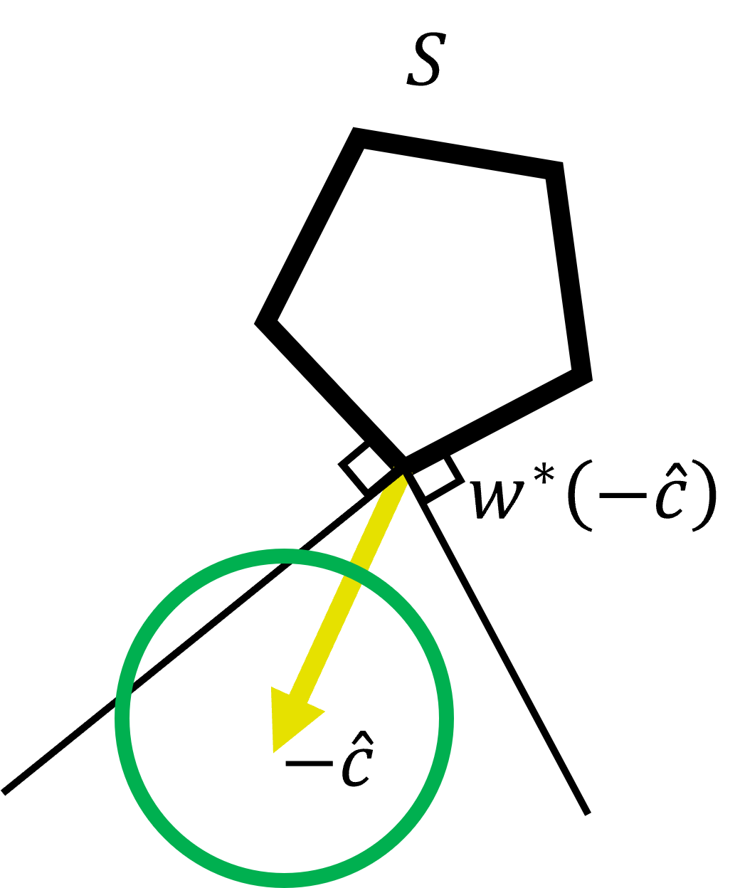
(a) Confidence region is large

(b) Confidence region is small

Figure 1: Active learning reduces the label complexity, given the same prediction.

Figure 2 further shows that considering the SPO loss function reduces the label complexity when the confidence regions of the cost vector are the same size. In Figure 2, both green circles have the same radius but their locations are different. In Figure 2(a), the confidence region for $\mathbb{E}[c|x]$ is close to the degenerate cost vectors, and thus the cost vectors within the confidence region will lead to multiple optimal decisions. In Figure 2(b), the confidence region for $\mathbb{E}[c|x]$ is far from the degenerate cost vectors, and therefore acquiring a label for $x$ is less informative, as we are more confident that $\hat{h}(x)$ leads to the correct optimal decision due to the more central location of the confidence region.

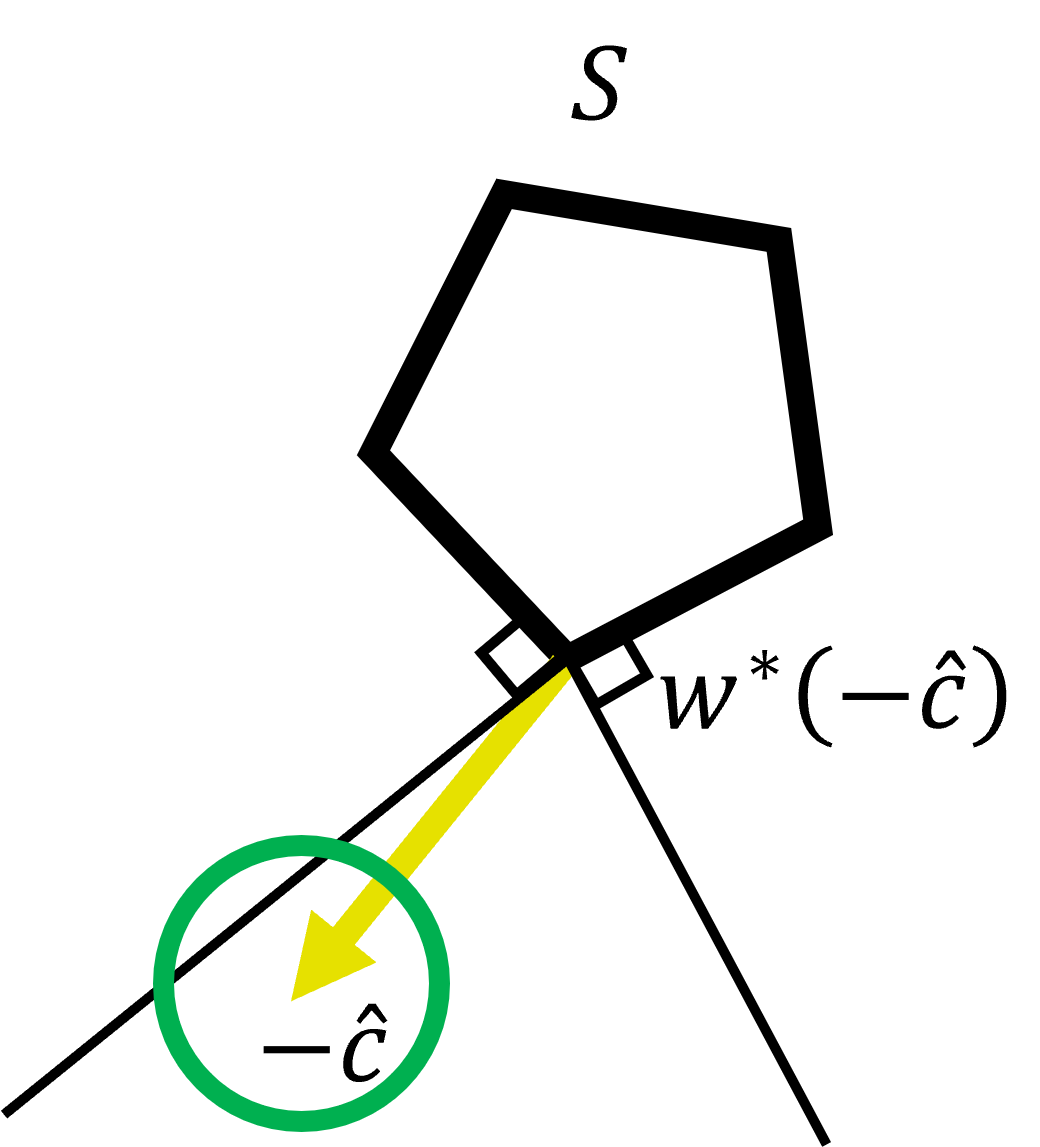
(a) Prediction is close to degenerate cost vectors

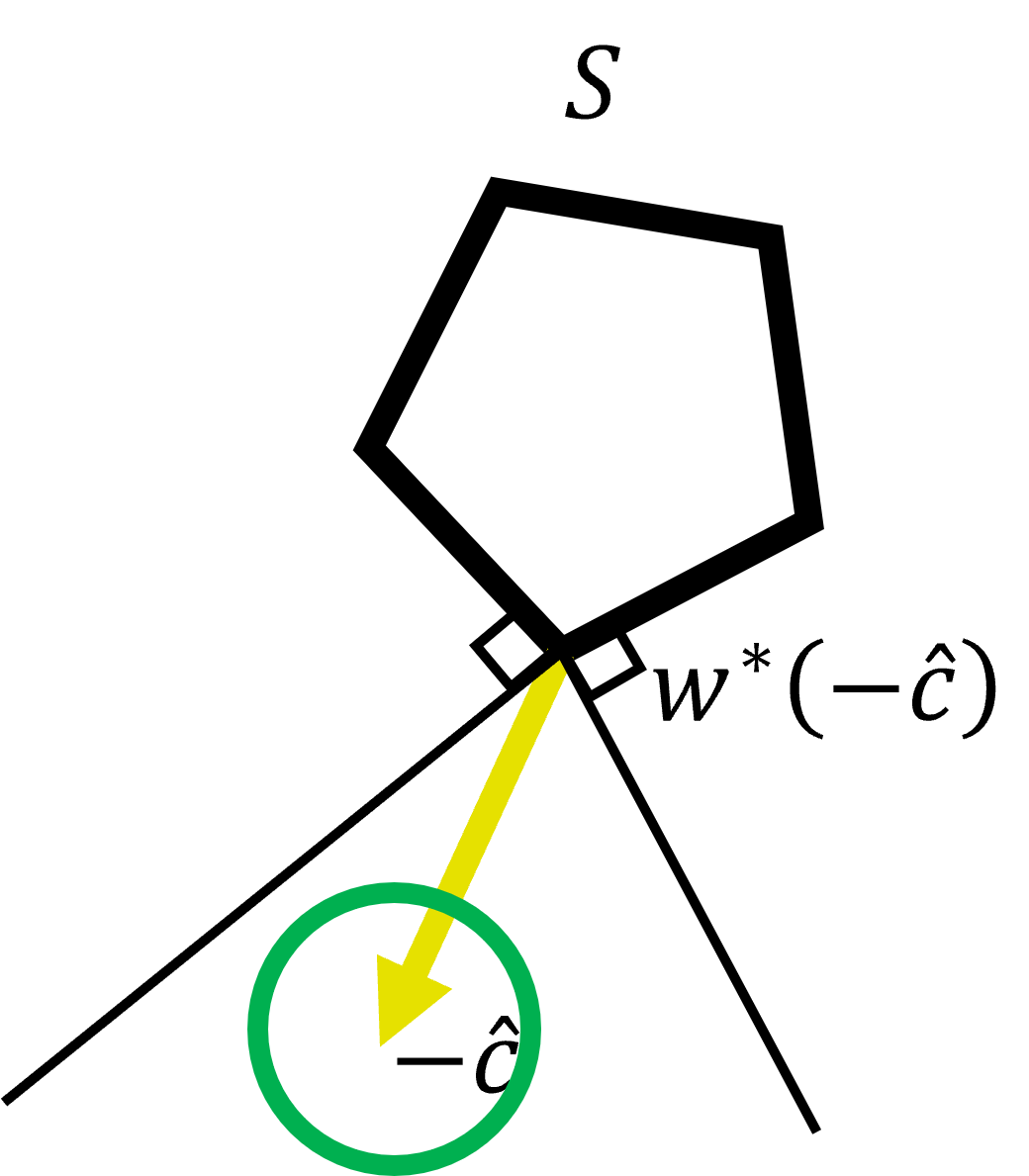
(b) Prediction is far from degenerate cost vectors

Figure 2: The SPO loss function reduces the label complexity, given the same size confidence region.

The above two examples highlight that the confidence associated with a prediction $\hat{h}(x)$ is crucial to determine whether it is valuable to acquire a true label $c$ associated with $x$. Furthermore, confidence is related to both the size of the confidence region (which is often dictated by the number of labeled samples we have acquired) and the location of the prediction relative to the structure of $S$. El Balghiti et al. (2022) introduced the notion of “distance to degeneracy,” which precisely measures the distance of a prediction $\hat{h}(x)$ to those degenerate cost vectors with multiple optimal solutions and thus provides the correct way to measure confidence about the location of a prediction. In fact, El Balghiti et al. (2022) argue that the distance to degeneracy provides a notion of confidence associated with a prediction that generalizes the notion of “margin” in binary and multiclass classification problems. El Balghiti et al. (2022) use the distance to degeneracy to provide tighter generalization guarantees for the SPO loss and its associated margin loss. In our context, we adopt the distance to degeneracy in order to determine whether or not to acquire labels. It is motivated by our intuition from the previously discussed examples wherein the labels of samples should be more informative if their predicted cost vectors are closer to degeneracy. In turn, we develop a generalization of margin-based active learning algorithms that utilize the distance to degeneracy as a confidence measure to determine those samples whose labels should (or should not) be acquired. Definition 3.1 reviews the notion of distance to degeneracy as defined by El Balghiti et al. (2022).

Definition 3.1

(Distance to Degeneracy, El Balghiti et al. (2022)). The set of degenerate cost vector predictions is $\mathcal{C}^{o}:=\{\hat{c}\in\mathbb{R}^{d}:P(\hat{c})$ has multiple optimal solutions$\}$. Given a norm $\|\cdot\|$ on $\mathbb{R}^{d}$, the distance to degeneracy of the prediction $\hat{c}$ is $\nu_{S}(\hat{c}):=\inf_{c\in\mathcal{C}^{o}}\{\|c-\hat{c}\|\}$.

The distance to degeneracy can be easily computed in some special cases, for example, when the feasible region $S$ is strongly convex or in the case of a polyhedral feasible region with known extreme point representations. El Balghiti et al. (2022) provide the exact formulas of the distance to degeneracy function in these two special cases. In particular, in the case of a polyhedral feasible region with extreme points $\{v_{j}:j=1,...,K\}$, that is, $S=\text{conv}(v_{1},\ldots,v_{K})$, Theorem 8 of El Balghiti et al. (2022) says that the distance to degeneracy of any vector $c\in\mathbb{R}^{d}$ satisfies the following equation:

$$\nu_{S}(c)=\min_{j:v_{j}\not=w^{*}(c)}\left\{\frac{c^{T}(v_{j}-w^{*}(c))}{\|v_{j}-w^{*}(c)\|_{*}}\right\}.$$ (4)

Theorem 7 of El Balghiti et al. (2022), on the other hand, says that $\nu_{S}(c)=\|c\|$ whenever $S$ is a strongly convex set. As mentioned, the distance to degeneracy $\nu_{S}(\hat{c})$ provides a measure of “confidence” regarding the cost vector prediction $\hat{c}$ and its implied decision $w^{*}(\hat{c})$. This observation motivates us to design a margin-based active learning algorithm, whereby if the distance to degeneracy $\nu_{S}(\hat{c})$ is greater than some threshold (depending on the number of iterations and samples acquired so far), then we are confident enough to label it using our current model without asking for the true label.

Our margin-based method is proposed in Algorithm 1. The idea of the margin-based algorithm can be explained as follows. At iteration $t$, we first observe an unlabeled feature vector $x_{t}$, which follows distribution $\mathcal{D}_{\mathcal{X}}$. Given the current predictor $h_{t-1}$, we calculate the distance to the degeneracy $\nu_{S}(h_{t-1}(x_{t}))$ of this unlabeled sample $x_{t}$. If the distance to degeneracy $\nu_{S}(h_{t-1}(x_{t}))$ is greater than the threshold $b_{t-1}$, then we reject $x_{t}$ with some probability $1-\tilde{p}$. If $\tilde{p}=0$, this rejection is referred to as a hard rejection; when $\tilde{p}>0$, this rejection is referred to as a soft rejection. If a soft-rejected sample is not ultimately rejected, we acquire a label (cost vector) $c_{t}$ associated with $x_{t}$ and add the sample $(x_{t},c_{t})$ to the set $\tilde{W}_{t}$. On the other hand, if $\nu_{S}(h_{t-1}(x_{t}))<b_{t-1}$, then we acquire a label (cost vector) $c_{t}$ associated with $x_{t}$ and add the sample $(x_{t},c_{t})$ to the working training set $W_{t}$. At each iteration, we update the predictor $h_{t}$ by computing the best predictor within a subset of the hypothesis class $H_{t}\subseteq\mathcal{H}$ that minimizes the empirical surrogate risk measured on the labeled samples. Note that Algorithm 1 maintains two working sets, $\tilde{W}_{t}$ and $W_{t}$, due to the two different types of labeling criteria. To ensure that the expectation of empirical loss is equal to the expectation of the true loss, we need to assign weight $\frac{1}{\tilde{p}}$ to the soft-rejection samples in the set $\tilde{W}_{t}$. It is assumed throughout that the sequence $(x_{1},c_{1}),(x_{2},c_{2}),\ldots$ is an i.i.d. sequence from the distribution $\mathcal{D}$.

Two versions of the MBAL-SPO have their own advantages. When using hard rejection, we update the set of predictors $H_{t}$ according to Line 20 in Algorithm 1, and the value of $\tilde{p}$ is set to zero. In contrast, in the soft rejection case, we keep $H_{t}$ as the entire hypothesis class $\mathcal{H}$ for all iterations, and the value of $\tilde{p}$ is non-zero. In comparison, hard rejection can result in a smaller label complexity because $\tilde{p}=0$, while soft rejection can reduce computational complexity by keeping $H_{t}$ as the whole hypothesis class $\mathcal{H}$. Please see the discussion in Sections 4.2 and 4.4 for further details.

In Algorithm 1, the case where $\nu_{S}(h_{t-1}(x_{t}))\geq b_{t-1}$ intuitively corresponds to the case where the confidence region of $h_{t-1}(x_{t})$ does not intersect with the degenerate cost vectors. Hence, we are sufficiently confident that the optimal decision $w^{*}(h_{t}(x_{t}))$ is equal to $w^{\ast}(h^{\ast}(x_{t}))$, where $h^{\ast}$ is a model that minimizes the SPO risk. Thus, we do not have to ask for the label of $x_{t}$. Lemma 3.2 further characterizes the conditions when two predictions lead to the same decision when the feasible region $S$ is polyhedral.

Lemma 3.2 (Conditions for identical decisions in polyhedral feasible regions.)

Suppose that the feasible region $S$ is polyhedral. Given two cost vectors $c_{1},c_{2}\in\mathbb{R}^{d}$, if $\|c_{1}-c_{2}\|<\max\{\nu_{S}(c_{1}),\nu_{S}(c_{2})\}$, then it holds that $w^{*}(c_{1})=w^{*}(c_{2})$. In other words, the optimal decisions for $c_{1}$ and $c_{2}$ are the same.

Lemma 3.2 implies that given one prediction of the cost vector, when its distance to degeneracy is larger than the radius of its confidence region, then all the predictions within this confidence region will lead to the same decision. Moreover, if the optimal prediction is also within this confidence region, the SPO loss of this prediction is zero.

The computational complexity of Algorithm 1 depends on the choice of the surrogate loss we use. As discussed earlier, calculating the distance to degeneracy $\nu_{S}(h(x))$ is efficient in some special cases. In general, in the polyhedral case when a convex hull representation is not available, a reasonable heuristic is to only compute the minimum in (4) with respect to the neighboring extreme points of $w^{*}(c)$. Alternatively, we observe that the objective inside the minimum in (4) is quasiconcave. Therefore, we can relax the condition that $v_{j}$ be an extreme point and still recover an extreme point solution. One can solve the resulting problem with a Frank-Wolfe type method, for example, see Yurtsever and Sra (2022). The computational complexity of updating $h_{t}$ in Line 19 depends on the choice of hypothesis class $\mathcal{H}$. In the case of soft rejection, we maintain $H_{t}=\mathcal{H}$ for all $t$ and the update is the same as performing empirical risk minimization in $\mathcal{H}$, which can be efficiently computed exactly or approximately for most common choices of $\mathcal{H}$, including linear and nonlinear models. In the case of hard rejections, $H_{t}$ is now the intersection of $t$ different level sets. Thus, $\min_{h\in H_{t}}\hat{\ell}^{t}(h)$ is a minimization problem with $t$ level set constraints. The complexity of solving this problem again depends on the choice of $\mathcal{H}$ and can often be solved efficiently. For example, in the case of linear models or nonlinear models such as neural networks, a viable approach would be to apply stochastic gradient descent to a penalized version of the problem or to apply a Lagrangian dual-type algorithm. In practice, since the constraints may be somewhat loose, we may simply ignore them and still obtain good results. Finally, we note that in both cases of hard rejection and soft rejection, although we have to solve a different optimization problem at every iteration, these optimization problems do not change much from one iteration to the next, and therefore using a warm-start strategy that uses $h_{t-1}$ as the initialization for calculating $h_{t}$ will be very effective.

Algorithm 1 Margin-Based Active Learning for SPO (MBAL-SPO)

1:  Input: Exploration probability $\tilde{p}$, a sequence of cut-off values $\{b_{t}\}$, a sequence $\{r_{t}\}$, and a constant $\vartheta$.

2:  Initialize the working sets $W_{0}\leftarrow\emptyset$, $\tilde{W}_{0}\leftarrow\emptyset$ and $H_{0}\leftarrow\mathcal{H}$.

3:  Arbitrarily pick one $h_{0}\in\mathcal{H}$, $n_{0}\leftarrow 0$.

4:  for $t$ from $1,2,...,T$ do

5:     Draw one sample $x_{t}$ from $\mathcal{D}_{\mathcal{X}}$.

6:     if $\nu_{S}(h_{t-1}(x_{t}))\geq b_{t-1}$ then

7:        Flip a coin with heads-up probability $\tilde{p}$.

8:        if  the coin gets heads-up then

9:           Acquire a “true” label $c_{t}$ of $x_{t}$.

10:           Update working set $\tilde{W}_{t}\leftarrow\tilde{W}_{t-1}\cup\{(x_{t},c_{t})\}$. Set $n_{t}\leftarrow n_{t-1}+1$.

11:        else

12:           Reject $x_{t}$. Set $n_{t}\leftarrow n_{t-1}$ and $\tilde{W}_{t}\leftarrow\tilde{W}_{t-1}$.

13:        end if

14:     else

15:        Acquire a “true” label $c_{t}$ of $x_{t}$.

16:        Update working set $W_{t}\leftarrow W_{t-1}\cup\{(x_{t},c_{t})\}$. Set $n_{t}\leftarrow n_{t-1}+1$.

17:     end if

18:     Let $\hat{\ell}^{t}(h)\leftarrow\frac{1}{t}\left(\sum_{(x,c)\in W_{t}}\ell(h(x),c)+\frac{1}{\tilde{p}}\sum_{(x,c)\in\tilde{W}_{t}}\ell(h(x),c)\right)$.

19:     Update $h_{t}\leftarrow\arg\min_{h\in H_{t-1}}\hat{\ell}^{t}(h)$ and $\hat{\ell}^{t,*}\leftarrow\min_{h\in H_{t-1}}\hat{\ell}^{t}(h)$.

20:     Optionally update the confidence set of the predictor $H_{t}$ by $H_{t}\leftarrow\{h\in H_{t-1}:\hat{\ell}^{t}(h)\leq\hat{\ell}^{t,*}+r_{t}+\frac{\vartheta}{t}\sum_{i=0}^{t-1}b_{i}^{2}\}$.

21:  end for

22:  Return $h_{T}$.

3.1.1 Surrogate Loss Function and Noise Distribution

Without further assumptions on the distribution of noise and features, the label complexity of an active learning algorithm can be the same as the sample complexity of supervised learning, as shown in Kääriäinen (2006). Therefore, we make several natural assumptions in order to analyze the convergence and label complexity of our algorithm. Recall that the optimal SPO and surrogate risk values are defined as:

$$R^{*}_{\textnormal{SPO}}:=\min_{h\in\mathcal{H}}\ R_{\textnormal{SPO}}(h),\ \ \text{and}\ \ \ R^{*}_{\ell}:=\min_{h\in\mathcal{H}}\ R_{\ell}(h).$$

We define $\mathcal{H}^{*}$ as the set of all optimal predictors for the SPO risk, i.e., $\mathcal{H}^{*}=\{h\in\mathcal{H}:R_{\textnormal{SPO}}(h)\leq R_{\textnormal{SPO}}(h^{\prime}),$ for all $h^{\prime}\in\mathcal{H}\}$ and $\mathcal{H}^{*}_{\ell}$ as the set of all optimal predictors for the risk of the surrogate loss, i.e., $\mathcal{H}^{*}_{\ell}=\{h\in\mathcal{H}:R_{\ell}(h)\leq R_{\ell}(h^{\prime}),$ for all $h^{\prime}\in\mathcal{H}\}$. We also use the notation $R^{*}_{\mathrm{SPO}+}$ and $\mathcal{H}^{*}_{\mathrm{SPO}+}$ when the surrogate loss $\ell$ is SPO+. We define the essential sup norm of a function $h:\mathcal{X}\to\mathbb{R}^{d}$ as $\|h\|_{\infty}:=\inf\{\alpha\geq 0:\|h(x)\|\leq\alpha\text{ for almost every }x\in\mathcal{X}\}$, with respect to the marginal distribution of $x$ and where $\|\cdot\|$ is the norm defining the distance to degeneracy (Definition 3.1). Given a set $\mathcal{H}^{\prime}\subseteq\mathcal{H}$, we further define the distance between a fixed predictor function $h$ and $\mathcal{H}^{\prime}$ as $\text{Dist}_{\mathcal{H}^{\prime}}(h):=\inf_{h^{\prime}\in\mathcal{H}^{\prime}}\{\|h-h^{\prime}\|_{\infty}\}$. Assumption 3.1.1 states our main assumptions on the surrogate loss function $\ell$ that we work with.

[Consistency and error bound condition] The hypothesis class $\mathcal{H}$ is a nonempty compact set w.r.t. to the sup norm, and the surrogate loss function $\ell:\mathbb{R}^{d}\times\mathbb{R}^{d}\rightarrow\mathbb{R}_{+}$ is continuous and satisfies:

1. $\mathcal{H}^{*}_{\ell}\subseteq\mathcal{H}^{*}$, i.e., the minimizers of the surrogate risk are also minimizers of the SPO risk.

2. There exists a non-decreasing function $\phi:\mathbb{R}_{+}\rightarrow\mathbb{R}_{+}$ with $\phi(0)=0$ such that for any $h\in\mathcal{H}$, for any $\epsilon>0$,

   $$R_{\ell}(h)-R_{\ell}^{*}\leq\epsilon~{}\Rightarrow~{}\mathrm{Dist}_{\mathcal{H}^{*}_{\ell}}(h)\leq\phi(\epsilon).$$

Assumption .(1) states the consistency of the surrogate loss function. Note that since $\mathcal{H}$ is a nonempty compact set and $\ell$ is a continuous function, $\mathcal{H}^{*}_{\ell}$ is also a nonempty compact set. On the other hand, the SPO loss is generally discontinuous so $\mathcal{H}^{*}$ is not necessarily compact, although the consistency assumption $\mathcal{H}^{*}_{\ell}\subseteq\mathcal{H}^{*}$ ensures that $\mathcal{H}^{*}$ is nonempty. Assumption .(2) is a type of error bound condition on the risk of the surrogate loss, wherein the function $\phi$ provides an upper bound of the sup norm between the predictor $h$ and the set of optimal predictors $\mathcal{H}_{\ell}^{*}$ whenever the surrogate risk of $h$ is close to the minimum surrogate risk value. By Assumption .(2), when the excess surrogate risk of $h$ becomes smaller, $h$ becomes closer to the set $\mathcal{H}_{\ell}^{*}$, which implies that the prediction $h(x)$ also gets closer to an optimal prediction $h^{*}(x)$ for any given $x$. As a consequence, the distance to degeneracy $\nu_{S}(h(x))$ also converges to $\nu_{S}(h^{*}(x))$ for almost all $x\in\mathcal{X}$. This property enables us to analyze the performance of MBAL-SPO under SPO+ and surrogate loss function respectively in the next two sections. Assumption 3.1.1 is related to the uniform calibration property studied in Ho-Nguyen and Kılınç-Karzan (2022) in the SPO context. Next, to measure how the density of the distribution $\nu_{S}(h^{\ast}(x))$ is allocated near the points of degeneracy, we define the near-degeneracy function $\Psi$ in Definition 3.3.

Definition 3.3 (Near-degeneracy function)

The near-degeneracy function $\Psi:\mathbb{R}_{+}\to[0,1]$ with respect to the distribution of $x\sim\mathcal{D}_{\mathcal{X}}$ is defined as:

$$\Psi(b):=\mathbb{P}\left(\inf_{h^{*}\in\mathcal{H}^{*}}\{\nu_{S}(h^{\ast}(x))\}\leq b\right).$$

The near-degeneracy function $\Psi$ measures the probability that the distance to degeneracy of $h^{*}(x)$ is smaller than $b$, when $x$ follows the marginal distribution of $x$ in $\mathcal{D}_{\mathcal{X}}$. If $\mathcal{H}^{*}$ contains more than one optimal predictor, the near-degeneracy function $\Psi$ considers the distribution of the smallest distance to degeneracy of all optimal predictors $h^{*}$. Intuitively, when $\Psi(b)$ is smaller, the density allocated near the points of degeneracy becomes smaller, which means Algorithm 1 has a larger probability to reject samples, and achieves smaller label complexity. This intuition is characterized in Lemma 3.4.

Lemma 3.4 (Upper bound on the expected number of acquired labels)

Suppose that Assumption 3.1.1 holds. In Algorithm 1, if $h_{t}$ satisfies $\mathrm{Dist}_{\mathcal{H}^{*}_{\ell}}(h_{t})\leq b_{t}$ for all iterations $t\geq 0$, then the expected number of acquired labels after $T$ total iterations is at most $\tilde{p}T+\sum_{t=1}^{T}\Psi(2b_{t-1})$.

Lemma 3.4 provides an upper bound for the expected number of acquired labels up to time $t$, by utilizing the near-degeneracy function $\Psi$. Note that in the soft rejection case, if $\tilde{p}>0$ and $\tilde{p}$ is independent of $T$, Lemma 3.4 implies that this upper bound grows linearly in $T$. However, if we know the value of $T$ before running the algorithm, then this upper bound can be reduced to a sublinear order by setting $\tilde{p}$ as a function of $T$. On the other hand, if we can set $\tilde{p}=0$, i.e., in the hard rejection case, the upper bound in Lemma 3.4 is sublinear if $\sum_{t=1}^{T}\Psi(2b_{t})$ is sublinear. As will be shown later in Proposition 5.1, in the hard rejection case, we achieve a sublinear and sometimes even finite label complexity when the near-degeneracy function $\Psi$ satisfies certain conditions.

4 Guarantees and Analysis for the Margin-Based Algorithm

In this section, we analyze the convergence and label complexity of MBAL-SPO in various settings. We first review some preliminary information about sequential complexity and covering numbers in Section 4.1. Next, we analyze the label complexity under hard rejections and soft rejections in Sections 4.2 and 4.4, respectively. In both sections, we develop non-asymptotic surrogate and SPO risk error bounds. We also develop bounds for the label complexity that, under certain conditions, can be much smaller than supervised learning. In Section 4.3, we further provide tighter SPO+ and SPO risk bounds when using the SPO+ surrogate under a separability condition. At the end of this section, we discuss how to set the values of the parameters in practice in MBAL-SPO. All missing proofs are provided in the appendix.

4.1 Preliminaries About Sequential Complexity

In Algorithm 1, the samples in the training set are not i.i.d., instead, whether to acquire the label at iteration $t$ depends on the historical label results. One of the challenges in analyzing the convergence and label complexity of the margin-based algorithm stems from the non i.i.d. samples. In this section, we review some techniques that characterize the convergence of non i.i.d. random sequences.

In Algorithm 1, the random variables in one iteration can be written as $(x_{t},c_{t},d^{M}_{t},q_{t})$, where $d^{M}_{t}\in\{0,1\}$ represents whether the sample is near degeneracy or not, i.e. if $\nu_{S}(h_{t-1}(x_{t}))<b_{t-1}$ then $d^{M}_{t}=1$, otherwise $d^{M}_{t}=0$. The random variable $q_{t}\in\{0,1\}$ represents the outcome of the coin flip that determines if we acquire the label of this sample or not, in the case when $d^{M}_{t}=0$. For simplicity, we use random variable $z_{t}\in\mathcal{Z}:=\mathcal{X}\times\mathcal{C}\times\{0,1\}\times\{0,1\}$ to denote the tuple of random variables $z_{t}:=(x_{t},c_{t},d^{M}_{t},q_{t})$. Thus, $z_{t}$ depends on $z_{1},...,z_{t-1}$ and the classical convergence results for i.i.d. samples do not apply in the margin-based algorithm. We define $\mathcal{F}_{t-1}$ as the $\sigma$-field of all random variables until the end of iteration $t-1$ (i.e., $\{z_{1},...,z_{t-1}\}$). In Algorithm 1, the re-weighted loss function at iteration $t$ is $\ell^{\mathtt{rew}}(h;z_{t}):=d^{M}_{t}\ell(h(x_{t}),c_{t})+(1-d^{M}_{t})q_{t}\frac{\mathbb{I}\{\tilde{p}>0\}}{\tilde{p}}\ell(h(x_{t}),c_{t})$. It is easy to see that $\ell^{\mathtt{rew}}(h;z)$ is upper bounded by $\frac{\omega_{\ell}(\hat{\mathcal{C}},\mathcal{C})}{\tilde{p}^{\mathbb{I}\{\tilde{p}>0\}}}<\infty$.

Then, to analyze the convergence of $\frac{1}{T}\sum_{t=1}^{T}\ell^{\mathtt{rew}}(h;z_{t})$ to $\frac{1}{T}\sum_{t=1}^{T}\mathbb{E}[\ell^{\mathtt{rew}}(h;z_{t})|\mathcal{F}_{t-1}]$, we adopt the sequential covering number defined in Rakhlin et al. (2015b). This notion generalizes the classical Rademacher complexity by defining a stochastic process on a binary tree. Let us briefly review the relevant results from Rakhlin et al. (2015b). A $\mathcal{Z}$-valued tree $\mathbf{z}$ of depth $T$ is a rooted complete binary tree with nodes labeled by elements of $\mathcal{Z}$. A path in the tree $\mathbf{z}$ is denoted by $\boldsymbol{\sigma}=(\sigma_{1},...,\sigma_{T})$, where $\sigma_{t}\in\{\pm 1\}$, for all $t\in\{1,\ldots,T\}$, with $\sigma_{t}=-1$ representing the left child node, and $\sigma_{t}=+1$ representing the right child node. The tree $\mathbf{z}$ is identified with the sequence $\mathbf{z}=(\mathbf{z}_{1},...,\mathbf{z}_{T})$ of labeling functions $\mathbf{z}_{i}:\{\pm 1\}^{i-1}\rightarrow\mathcal{Z}$ which provide the labels for each node. Therefore, $\mathbf{z}_{1}\in\mathcal{Z}$ is the label for the root of the tree, while $\mathbf{z}_{i}$ for $i>1$ is the label of the node obtained by following the path of length $i-1$ from the root. In a slight abuse of notation, we use $\mathbf{z}_{i}(\boldsymbol{\sigma})$ to refer to the label of the $i^{\mathrm{th}}$ node along the path defined by $\boldsymbol{\sigma}$. Similar to a $\mathcal{Z}$-valued tree $\mathbf{z}$, a real-valued tree $\boldsymbol{v}=(\boldsymbol{v}_{1},...,\boldsymbol{v}_{T})$ of depth $T$ is a tree identified by the real-valued labeling functions $\boldsymbol{v}_{i}:\{\pm 1\}^{i-1}\rightarrow\mathbb{R}$. Thus, given any loss function $\ell(h;\cdot):\mathcal{Z}\rightarrow\mathbb{R}$, the composition $\ell(h;\cdot)\circ\mathbf{z}$ is a real-valued tree given by the labeling functions $(\ell(h;\cdot)\circ\boldsymbol{z}_{1},\ell(h;\cdot)\circ\boldsymbol{z}_{2},...,\ell(h;\cdot)\circ\boldsymbol{z}_{T})$ for any fixed $h\in\mathcal{H}$.

Definition 4.1 (Sequential covering number)

(Rakhlin et al. (2015b), Kuznetsov and Mohri (2015)) Let $\ell(h;\mathbf{z})$ denote the loss of predictor $h$ given the random variable $\mathbf{z}$. Given a $\mathcal{Z}$-valued tree $\mathbf{z}$ of depth $T$, a set $V$ of real-valued trees of depth $T$ is a sequential $\alpha$-cover, with respect to the $\ell_{1}$ norm, of a function class $\mathcal{H}$ with respect to the loss $\ell$ if for all $h\in\mathcal{H}$ and for all paths $\boldsymbol{\sigma}\in\{\pm 1\}^{T}$, there exists a real-valued tree $\boldsymbol{v}\in V$ such that

$$\sum_{t=1}^{T}|\boldsymbol{v}_{t}(\boldsymbol{\sigma})-\ell(h;\boldsymbol{z}_{t}(\boldsymbol{\sigma}))|\leq T\alpha.$$

The sequential covering number $N_{1}(\alpha,\ell\circ\mathcal{H},\boldsymbol{z})$ of a function class $\mathcal{H}$ with respect to the loss $\ell$ is defined to be the cardinality of the minimal sequential cover. The maximal covering number is then taken to be $N_{1}(\alpha,\ell\circ\mathcal{H},T):=\sup_{\boldsymbol{z}}\{N_{1}(\alpha,\ell\circ\mathcal{H},\boldsymbol{z})\}$, where the supremum is over all $\mathcal{Z}$-valued trees $\mathbf{z}$ of depth $T$.

In Definition 4.1, the loss function $\ell$ can be either the reweighted loss $\ell^{\mathtt{rew}}$ or the surrogate loss. In comparison, the standard covering number for i.i.d. observations $\hat{N_{1}}(\alpha,\ell\circ\mathcal{H})$ is defined as

$$\hat{N_{1}}(\alpha,\ell\circ\mathcal{H}):=\inf\{|V|:V\subseteq\mathbb{R}^{\mathcal{Z}}\text{ s.t. }\forall h\in\mathcal{H},\exists v\in V\text{ with }\sup_{\mathbf{z}\in\mathcal{Z}}\{|v(\mathbf{z})-\ell(h;\mathbf{z})|\}\leq\alpha\}.$$

Utilizing the sequential covering number, Kuznetsov and Mohri (2015) provides a data-dependent generalization error bound for non i.i.d. sequences. As a relaxed version of their results, the data-independent error bound is stated in Proposition 4.2. This proposition is from the last line of proof of Theorem 1 in Kuznetsov and Mohri (2015), and we apply it to the reweighted loss.

Proposition 4.2 (Non i.i.d. generalization error bound)

(Theorem 1 in Kuznetsov and Mohri (2015)) Let $\{z_{1},z_{2},...z_{T}\}$ be a (non i.i.d.) sequence of random variables. Fix $\epsilon>2\alpha>0$. Then, the following holds:

$$\mathbb{P}\left(\sup_{h\in\mathcal{H}}\left\{\left|\frac{1}{T}\sum_{t=1}^{T}\left(\mathbb{E}[\ell^{\mathtt{rew}}(h;z_{t})|\mathcal{F}_{t-1}]-\ell^{\mathtt{rew}}(h;z_{t})\right)\right|\right\}\geq\epsilon\right)\leq 2N_{1}(\alpha,\ell^{\mathtt{rew}}\circ\mathcal{H},T)\exp\left\{-\frac{\tilde{p}^{2\mathbb{I}\{\tilde{p}>0\}}T(\epsilon-2\alpha)^{2}}{2\omega_{\ell}(\hat{\mathcal{C}},\mathcal{C})^{2}}\right\}.$$

Proposition 4.3 further provides an upper bound for $N_{1}(\alpha,\ell^{\mathtt{rew}}\circ\mathcal{H},T)$ when $\mathcal{H}$ is a smoothly-parameterized class.

Proposition 4.3 (Bound for the sequential covering number)

Suppose $\mathcal{H}$ is a class of functions smoothly-parameterized by $\theta\in\Theta\subseteq\mathbb{R}^{d_{\theta}}$ with respect to the $\ell_{\infty}$ norm, i.e., there exists $L_{1}>0$ such that for any $\theta_{1},\theta_{2}\in\Theta$ and any $x\in\mathcal{X}$, $\|h_{\theta_{1}}(x)-h_{\theta_{2}}(x)\|_{\infty}\leq L_{1}\|\theta_{1}-\theta_{2}\|_{\infty}$. Let $\rho(\Theta)$ be the diameter of $\Theta$ in the $\ell_{\infty}$ norm. Suppose the surrogate loss function $\ell(\cdot,c)$ is $L_{2}$-Lipschitz with respect to the $\ell_{\infty}$ norm for any fixed $c$. Then, given $\tilde{p}$, for any $\alpha>0$, for any $T\geq 1$, we have that

$$\ln(N_{1}(\alpha,\ell^{\mathtt{rew}}\circ\mathcal{H},T))\leq d_{\theta}\ln\left(1+\frac{2\rho(\Theta)L_{1}L_{2}}{\alpha\tilde{p}^{\mathbb{I}\{\tilde{p}>0\}}}\right)\leq\mathcal{O}\left(\ln\left(\frac{1}{\alpha\tilde{p}^{\mathbb{I}\{\tilde{p}>0\}}}\right)\right).$$

The smoothly-parameterized hypothesis class $\mathcal{H}$ is a common assumption when analyzing the covering number for parameterized class, e.g., see Assumption 3 in Gao (2022) and their examples. When hypothesis class $\mathcal{H}$ is smoothly parameterized, for example, a bounded class of linear functions, Proposition 4.3 implies that $N_{1}(\alpha,\ell^{\mathtt{rew}}\circ\mathcal{H},T)$ is upper bounded by $\mathcal{O}\left(\ln\left(\frac{1}{\alpha\tilde{p}^{\mathbb{I}\{\tilde{p}>0\}}}\right)\right)$, which is independent of $T$. Together with Proposition 4.2, it shows that $\frac{1}{T}\sum_{t=1}^{T}\ell^{\mathtt{rew}}(h;z_{t})$ converges to $\frac{1}{T}\sum_{t=1}^{T}\mathbb{E}[\ell^{\mathtt{rew}}(h;z_{t})|\mathcal{F}_{t-1}]$ at rate $\mathcal{\tilde{O}}(1/\sqrt{T})$.

4.2 MBAL-SPO with Hard Rejections

In this section, we develop excess risk bounds for the surrogate risk and the SPO risk, and present label complexity results, for MBAL-SPO with hard rejections. Our excess risk bounds for the surrogate risk hold for general feasible regions $S$. To develop risk bounds for the SPO risk, we consider two additional assumptions on $S$: (i) the case where $S$ satisfies the strength property, and (ii) the case where $S$ is polyhedral. The strength property, as defined in El Balghiti et al. (2022), is reviewed below in Definition 4.4.

Definition 4.4 (Strength Property for the Feasible Region $S$)

The feasible region $S$ satisfies the strength property with constant $\mu>0$ if, for all $w\in S$ and $\hat{c}\in\mathbb{R}^{d}$, it holds that

$$\hat{c}^{T}(w-w^{*}(\hat{c}))\geq\frac{\mu\cdot\nu_{S}(\hat{c})}{2}\|w-w^{*}(\hat{c})\|^{2},$$ (5)

where $\nu_{S}$ is the distance to degeneracy function. We refer to $\mu$ as the strength parameter.

The strength property can be interpreted as a variant of strong convexity that bounds the distance to the optimal solution based on the parameter $\mu$ as well as the distance to degeneracy $\nu_{S}(\hat{c})$. El Balghiti et al. (2022) demonstrate that the strength property holds when $S$ is polyhedral or a strongly convex set. In addition, for some of the results herein, we make the following assumption concerning the surrogate loss function, which states the uniqueness of the surrogate risk minimizer and a relaxation of Hölder continuity. [Unique minimizer and Hölder-like property] There is a unique minimizer $h^{*}$ of the surrogate risk, i.e., the set $\mathcal{H}_{\ell}^{*}$ is a singleton, and there exists a constant $\eta>0$ such that the surrogate loss function $\ell$ satisfies

$$\left|\mathbb{E}[\ell(\hat{c},c)-\ell(h^{*}(x),c)|x]\right|~{}\leq~{}\eta\|\hat{c}-h^{*}(x)\|^{2}\text{ for all }x\in\mathcal{X},\text{ and }\hat{c}\in\mathcal{\hat{C}}.$$

It is easy to verify that the common squared loss satisfies Assumption 4.4 with $\eta=1$ when the hypothesis class is well-specified. In Lemma 8.6 in Appendix 8, we further show that the SPO+ loss satisfies Assumption 4.4 under some noise conditions.

Theorem 4.5 is our main theorem concerning MBAL-SPO with hard rejections and with general surrogate losses satisfying Assumption 4.4. Theorem 4.5 presents bounds on the excess surrogate and SPO risks as well as the expected label complexity after $T$ iterations.

Theorem 4.5 (General surrogate loss, hard rejection)

Suppose that Assumptions 3.1.1 and 4.4 hold, and that Algorithm 1 sets $\tilde{p}\leftarrow 0$ and updates the set of predictors according to the optional update rule in Line 20 with $\vartheta\leftarrow\eta$. Furthermore in Algorithm 1, for a given $\delta\in(0,1]$, let $r_{0}\geq\omega_{\ell}(\hat{\mathcal{C}},\mathcal{C})$, $r_{t}\leftarrow 2\omega_{\ell}(\hat{\mathcal{C}},\mathcal{C})\left[\sqrt{\frac{4\ln(2tN_{1}(\omega_{\ell}(\hat{\mathcal{C}},\mathcal{C})/t,\ell^{\mathtt{rew}}\circ\mathcal{H},t)/\delta)}{t}}+\frac{2}{t}\right]$ for $t\geq 1$, $b_{0}\leftarrow\max\{\phi(r_{0}),\sqrt{r_{0}/\eta}\}$, and $b_{t}\leftarrow\phi(2r_{t}+\frac{2\eta}{t}\sum_{i=0}^{t-1}b_{i}^{2})$ for $t\geq 1$. Then, the following guarantees hold simultaneously with probability at least $1-\delta$ for all $T\geq 1$:

• (a) The excess surrogate risk satisfies $R_{\ell}(h_{T})-R_{\ell}^{*}\leq r_{T}+\frac{\eta}{T}\sum_{t=0}^{T-1}b_{t}^{2}$,

• (b) If the feasible region $S$ satisfies the strength property with parameter $\mu>0$, then the excess SPO risk satisfies

  $$R_{\textnormal{SPO}}(h_{T})-R_{\textnormal{SPO}}^{*}\leq\inf_{\gamma_{T}\geq 2b_{T}}\left\{\frac{2\rho(\mathcal{C})b_{T}}{\mu\gamma_{T}}+\Psi(\gamma_{T})\omega_{S}(\mathcal{C})\right\},$$

• (c) If the feasible region $S$ is polyhedral, then the excess SPO risk satisfies $R_{\textnormal{SPO}}(h_{T})-R_{\textnormal{SPO}}^{*}\leq\Psi(2b_{T})\omega_{S}(\mathcal{C})$,

• (d) The expectation of the number of labels acquired, $\mathbb{E}[n_{T}]$, deterministically satisfies $\mathbb{E}[n_{T}]\leq\sum_{t=1}^{T}\Psi(2b_{t-1})+\delta T$.

In the polyhedral case, Theorem 4.5 indicates that the excess SPO risk of Algorithm 4.5 converges to zero at rate $\mathcal{O}(\Psi(2b_{T}))$, and the expectation of the number of acquired labels grows at rate $\mathcal{O}\left(\sum_{t=1}^{T}\Psi(2b_{t})\right)$ for small $\delta$. (Usually, $\delta\ll\mathcal{O}(1/T)$.) Note that Theorem 4.5 is generic in that the excess risk and label complexity bounds depend on the functions $\phi$ and $\Psi$. In Appendix 8, we give the explicit forms of these functions in some special cases of interest.

Remark 4.6 (Updates of $H_{t}$)

In Theorem 4.5, the set of predictors is updated according to Line 20 in Algorithm 1. This is a technical requirement for the convergence when setting $\tilde{p}=0$. This update process means that $h_{t}\in H_{t-1}\subseteq H_{t-2}...\subseteq H_{0}=\mathcal{H}$. By constructing these shrinking sets $H_{t}$ of predictors, we are able to utilize the information from previous iterations. Particularly, Lemma 4.9 below shows that these shrinking sets $H_{t-1}$ always contain the true optimal predictor $h^{*}$ under certain conditions.

Remark 4.7 (Value of $\gamma_{T}$)

In Theorem 4.5, to find the best value of the parameter $\gamma_{T}$ in part (b) that minimizes the excess SPO risk for sets satisfying the strength property, we observe that the choice of $\gamma_{T}$ depends on $\Psi$, $\phi$ and $T$. If $\gamma_{T}$ satisfies that (1) $\frac{b_{T}}{\gamma_{T}}\rightarrow 0$, when $r_{T}\rightarrow 0$, and (2) $\gamma_{T}\rightarrow 0$, when $T\rightarrow\infty$, then the excess SPO risk will converge to zero. For example, we can set $\gamma_{T}=\left(b_{T}\right)^{\kappa}$, where $\kappa\in(0,1)$.

Auxiliary Results for the Proof of Theorem 4.5.

To achieve the risk bound in part (a) of Theorem 4.5, we decompose the excess surrogate risk into three parts. First, we denote the re-weighted surrogate risk for the features that are far away from degeneracy by $\ell^{\text{f}}_{t}(h)$, defined by:

$$\ell^{\mathrm{f}}_{t}(h):=\mathbb{E}[\ell(h;z_{t})\mathbb{I}\{\nu_{S}(h_{t-1}(x_{t}))\geq b_{t-1}\}|\mathcal{F}_{t-1}]=\mathbb{E}[\ell(h;z_{t})(1-d^{M}_{t})|\mathcal{F}_{t-1}],$$

where we use $\ell(h;z_{t})$ to denote $\ell(h(x_{t}),c_{t})$ and the expectation above is with respect to $z_{t}$. Since $x_{t}$ and $c_{t}$ are i.i.d. random variables, and only $d^{M}_{t}$ depends on $\mathcal{F}_{t-1}$, $\ell^{\text{f}}_{t}(h)$ can further be written as $\ell^{\text{f}}_{t}(h)=\mathbb{E}[\ell(h(x_{t}),c_{t})|d^{M}_{t}=0]\mathbb{P}(d^{M}_{t}=0|\mathcal{F}_{t-1})$. Note also that, since $\tilde{p}=0$, the re-weighted loss function can be written as $\ell^{\mathtt{rew}}(h;z_{t})=\ell(h(x_{t}),c_{t})d^{M}_{t}=\ell(h(x_{t}),c_{t})\mathbb{I}\{\nu_{S}(h_{t-1}(x_{t}))<b_{t-1}\}$, for a given $h\in\mathcal{H}$. Next, for given $h\in\mathcal{H}$ and $h^{\ast}\in\mathcal{H}^{\ast}_{\ell}$, we denote the discrepancy between the conditional expectation and the realized excess re-weighted loss of predictor $h$ at time $t$ by $Z^{\mathtt{t}}_{h}$, i.e., $Z^{\mathtt{t}}_{h}:=\mathbb{E}[\ell^{\mathtt{rew}}(h;z_{t})-\ell^{\mathtt{rew}}(h^{*};z_{t})|\mathcal{F}_{t-1}]-(\ell^{\mathtt{rew}}(h;z_{t})-\ell^{\mathtt{rew}}(h^{*};z_{t}))$. Lemma 4.8 shows that the excess surrogate risk can be decomposed into three parts.

Lemma 4.8 (Decomposition of the excess surrogate risk)

In the case of hard rejections, i.e., $\tilde{p}\leftarrow 0$ in Algorithm 1, for any given $h^{\ast}\in\mathcal{H}^{\ast}_{\ell}$ and $T\geq 1$, the excess surrogate risk of any predictor $h\in\mathcal{H}$ can be decomposed as follows:

$$R_{\ell}(h)-R_{\ell}(h^{\ast})~{}=~{}\frac{1}{T}\sum_{t=1}^{T}\left(\ell^{\mathrm{f}}_{t}(h)-\ell^{\mathrm{f}}_{t}(h^{*})\right)+\frac{1}{T}\sum_{t=1}^{T}Z^{\mathtt{t}}_{h}+\frac{1}{T}\sum_{t=1}^{T}\left(\ell^{\mathtt{rew}}(h;z_{t})-\ell^{\mathtt{rew}}(h^{*};z_{t})\right).$$

The first part in Lemma 4.8 is the averaged excess surrogate risk for the hard rejected features at each iteration. Lemma 4.9 below further shows that $\left|\ell^{\text{f}}_{t}(h)-\ell^{\text{f}}_{t}(h^{*})\right|$ is close to zero when $h\in H_{T-1}$.

Lemma 4.9

Suppose that Assumptions 3.1.1 and 4.4 hold where $h^{*}$ denotes the unique minimizer of the surrogate risk, and that Algorithm 1 sets $\tilde{p}\leftarrow 0$ and updates the set of predictors according to the optional update rule in Line 20 with $\vartheta\leftarrow\eta$. Furthermore, suppose that that $r_{0}\geq\omega_{\ell}(\hat{\mathcal{C}},\mathcal{C})$, $r_{t}\geq\sup_{h\in\mathcal{H}}\left\{\left|\frac{1}{t}\sum_{i=1}^{t}Z^{\mathtt{i}}_{h}\right|\right\}$ for $t\geq 1$, $b_{0}\leftarrow\max\{\phi(r_{0}),\sqrt{r_{0}/\eta}\}$, and $b_{t}\leftarrow\phi(2r_{t}+\frac{2\eta}{t}\sum_{i=0}^{t-1}b_{i}^{2})$ for $t\geq 1$. Then, for all $t\geq 1$, it holds that (a) $h^{*}\in H_{t-1}$, and (b) $\sup_{h\in H_{t-1}}\left\{\left|\ell^{\mathrm{f}}_{t}(h)-\ell^{\mathrm{f}}_{t}(h^{*})\right|\right\}\leq\eta b_{t-1}^{2}$.

With Lemma 4.9, we can appropriately bound the first average of terms in Lemma 4.8, involving the expected surrogate risk when far from degeneracy. Thus, Lemmas 4.8 and 4.9 enable us to prove the excess surrogate risk bound in part (a). The proofs of the remaining parts follow by translating the excess surrogate risk bound to guarantees on the excess SPO risk and the label complexity.

4.3 Refined Bounds for SPO+ Under Separability

Next, we provide a smaller excess risk bound when using SPO+ as the surrogate loss, again in the case of hard rejections. The SPO+ loss function incorporates the structure of the downstream optimization problem and, intuitively, the excess SPO+ risk when far away from degeneracy will be close to zero when the distance $\text{Dist}_{\mathcal{H}^{*}_{\ell}}(h)$ is small and the distribution satisfies a separability condition, which we define below.

[Strong separability condition] There exist constants $\varrho\in[0,1)$ and $\tau\in(0,1]$ such that, for all $h^{*}\in\mathcal{H}_{\mathrm{SPO}+}^{\ast}$, with probability one over $(x,c)\sim\mathcal{D}$, it holds that:

• (1) $\|h^{*}(x)-c\|\leq\varrho\nu_{S}(h^{*}(x))$, and

• (2) $\nu_{S}(h^{*}(x))\geq\tau\left(\sup_{h^{\prime}\in\mathcal{H}_{\mathrm{SPO}+}^{\ast}}\{\nu_{S}(h^{\prime}(x))\}\right)$.

The following proposition shows that the separability condition leads to zero SPO+ and SPO risk in the polyhedral case. Indeed, the SPO+ loss is a generalization of the hinge loss and the structured hinge loss in binary and multi-class classification problems and is expected to achieve zero loss when there is a predictor function $\bar{h}$ that strictly separates the cost vectors into different classes corresponding to the extreme points of $S$ (Elmachtoub and Grigas 2022). Assumption 4.3 and Proposition 4.10 formally define the notion of separability, wherein the distance between the prediction $\bar{h}(x)$ and the realized cost vector $c$, relative to the distance to degeneracy of $\bar{h}(x)$, is controlled.

Proposition 4.10 (Zero SPO+ risk in the polyhedral and separable case)

Assume that there exists $\bar{h}\in\mathcal{H}$ and a constant $\varrho\in[0,1)$ such that $\|\bar{h}(x)-c\|\leq\varrho\nu_{S}(\bar{h}(x))$ with probability one over $(x,c)\sim\mathcal{D}$. When the feasible region S is polyhedral, it holds that $R_{\textnormal{SPO+}}^{*}=R_{\textnormal{SPO}}^{*}=0$ and $\bar{h}$ is a minimizer for both $R_{\textnormal{SPO+}}$ and $R_{\textnormal{SPO}}$.

As compared to Theorem 4.5, Theorem 4.11 below presents improved surrogate risk convergence guarantees for SPO+ under separability in the polyhedral case.

Theorem 4.11 (SPO+ surrogate loss, hard rejection, polyhedral and separable case)

Suppose that the feasible region $S$ is polyhedral, Assumptions 3.1.1 and 4.3 hold, and the surrogate loss function is SPO+. Suppose that Algorithm 1 sets $\tilde{p}\leftarrow 0$ and $H_{t}\leftarrow\mathcal{H}$ for all $t$. Furthermore in Algorithm 1, for a given $\delta\in(0,1]$, let $r_{0}\geq\omega_{\ell}(\hat{\mathcal{C}},\mathcal{C})$, $r_{t}\leftarrow\omega_{\ell}(\hat{\mathcal{C}},\mathcal{C})\left[\sqrt{\frac{4\ln(2t\hat{N_{1}}(\omega_{\ell}(\hat{\mathcal{C}},\mathcal{C})/t,\ell_{\textnormal{SPO+}}\circ\mathcal{H})/\delta)}{t}}+\frac{2}{t}\right]$ for $t\geq 1$, $b_{0}\leftarrow\max\{\phi(r_{0}),\rho(\mathcal{\hat{C}})\}$, and $b_{t}\leftarrow(1+\frac{2}{\tau(1-\rho)})\phi(r_{t})$ for $t\geq 1$. Then, the following guarantees hold simultaneously with probability at least $1-\delta$ for all $T\geq 1$:

• (a) The excess SPO+ risk satisfies $R_{\textnormal{SPO+}}(h_{T})-R_{\textnormal{SPO+}}^{*}=R_{\textnormal{SPO+}}(h_{T})\leq r_{T}$,

• (b) The excess SPO risk satisfies $R_{\textnormal{SPO}}(h_{T})-R_{\textnormal{SPO}}^{*}=R_{\textnormal{SPO}}(h_{T})\leq\Psi(2b_{T})\omega_{S}(\mathcal{C})$,

• (c) The expectation of the number of labels acquired, $\mathbb{E}[n_{T}]$, deterministically satisfies $\mathbb{E}[n_{T}]\leq\sum_{t=1}^{T}\Psi(2b_{t-1})+\delta T$.

Remark 4.12 (Benefits of SPO+ Under Separability)

When using SPO+ in the separable case, the bound in part (a) of Theorem 4.11 is substantially improved as compared to Theorem 4.5. Intuitively, when an optimal predictor $h^{*}(x)$ is far away from degeneracy and $h_{t}(x)$ and $h^{*}(x)$ are close, then the excess SPO+ risk of $h_{t}(x)$ can be shown to be zero. As a result, the rejection criterion – which compares $\nu_{S}(h_{t}(x))$ to a quantity $b_{t}$ that is related to the distance between $h_{t}$ and $h^{*}$ – is “safe” in the sense that whenever $h_{t}(x)\geq b_{t}$ we can demonstrate that $h_{t}(x)$ leads to a correct optimal decision with high probability. Thus, when using the SPO+ loss function, we can obtain a smaller excess SPO+ risk bound. Indeed, in Theorem 4.11, the value of $r_{t}$ is determined by the i.i.d. covering number, which implies that this risk bound is the same as the risk bound of supervised learning that labels all the samples. Furthermore, another benefit of SPO+ under the separability assumption is that we do not need to update $H_{t}$ at each iteration, which simplifies the computation substantially. Finally, Assumption 4.4 which assumes the minimizer $h^{*}$ is unique is not needed.

Theorem 4.11 shows that the excess SPO+ risk converges to zero at rate $\mathcal{\tilde{O}}(1/\sqrt{T})$, which equals the typical learning rate for the excess SPO+ risk in supervised learning. As Algorithm 1 requires much fewer labels, this demonstrates the advantage of active learning. In fact, the main idea of the proof of Theorem 4.11 is to show that $h_{T}$ actually, with high probability, achieves zero empirical SPO+ risk over all samples $(x_{1},c_{1}),\ldots,(x_{T},c_{T})$ – including the cases where the label is not acquired. Indeed, in the separable case, the rejection criterion is “safe” and we are able to demonstrate that $\ell_{\textnormal{SPO+}}(h_{t}(x_{t}),c_{t})=0$ when $\nu_{S}(h_{t-1}(x_{t}))\geq b_{t-1}$. This of course implies that $h_{T}$ is an empirical risk minimizer for SPO+ across $T$ i.i.d. samples $(x_{1},c_{1}),\ldots,(x_{T},c_{T})$ and we are able to conclude part (a).

4.4 MBAL-SPO with Soft Rejections

In this section, we analyze the convergence and label complexity of MBAL-SPO with soft rejection. We return to the setting of a generic surrogate loss function $\ell$. Compared to the hard rejection case in Theorem 4.5, this positive $\tilde{p}$ will lead to a larger label complexity than Theorem 4.5. On the other hand, when $\tilde{p}$ is positive, we do not have to construct the confidence set $H_{t}$ of the predictors at each iteration. In other words, $H_{t}$ can be set as $\mathcal{H}$, for all $t$ as in Theorem 4.11. Thus, we do not have to consider $t$ additional constraints when minimizing the empirical re-weighted risk, which will reduce the computational complexity significantly. Theorem 4.13 is our main theorem for the MBAL-SPO under a general surrogate loss, which again provides upper bounds for the excess surrogate and SPO risk and label complexity of the algorithm.

Theorem 4.13 (General surrogate loss, soft rejection)

Suppose that Assumption 3.1.1 holds, and let $\delta\in(0,1]$ and $\tilde{p}\in(0,1]$ be given. In Algorithm 1, set $H_{t}\leftarrow\mathcal{H}$ for all $t\geq 0$, $r_{0}\geq\omega_{\ell}(\hat{\mathcal{C}},\mathcal{C})$, $r_{t}\leftarrow 2\omega_{\ell}(\hat{\mathcal{C}},\mathcal{C})\left[\frac{1}{\tilde{p}}\sqrt{\frac{2\ln(2N_{1}(\frac{\omega_{\ell}(\mathcal{\hat{C}},\mathcal{C})}{t},\ell^{\mathtt{rew}}\circ\mathcal{H},t)/\delta)}{t}}+\frac{2}{t}\right]$ for $t\geq 1$, $b_{t}\leftarrow 2\phi(r_{t})$ for $t\geq 0$. Then, the following guarantees hold simultaneously with probability at least $1-\delta$ for all $T\geq 1$:

• (a) The excess surrogate risk satisfies $R_{\ell}(h_{T})-R_{\ell}^{\ast}\leq r_{T}$,

• (b) If the feasible region $S$ satisfies the strength property with parameter $\mu>0$, then the excess SPO risk satisfies

  $$R_{\textnormal{SPO}}(h_{T})-R_{\textnormal{SPO}}^{*}\leq\inf_{\gamma_{T}\geq 2b_{T}}\left\{\frac{2\rho(\mathcal{C})b_{T}}{\mu\gamma_{T}}+\Psi(\gamma_{T})\omega_{S}(\mathcal{C})\right\},$$

• (c) If the feasible region $S$ is polyhedral, then the excess SPO risk satisfies $R_{\textnormal{SPO}}(h_{T})-R_{\textnormal{SPO}}^{*}\leq\Psi(2b_{T})\omega_{S}(\mathcal{C})$,

• (d) The expectation of the number of labels acquired, $\mathbb{E}[n_{T}]$, deterministically satisfies $\mathbb{E}[n_{T}]\leq\tilde{p}T+\sum_{t=1}^{T}\Psi(2b_{t-1})+\delta T$.

Remark 4.14 (Value of $b_{t}$ and $\tilde{p}$)

In part (d) of Theorem 4.13, $\mathbb{E}[n_{T}]$ depends on both $\tilde{p}T$ and $\sum_{t=1}^{T}\Psi(2b_{t})$. When the exploration probability $\tilde{p}$ is large, $\tilde{p}T$ in part (d) of Theorem 4.13 is large. On the other hand, in Theorem 4.13, the value of $b_{t}$ depends on $r_{t}$, and $r_{t}$ furthermore is in the order of $O(1/\tilde{p})$. It implies that when the exploration probability $\tilde{p}$ is small, $b_{t}$ is large, and $\sum_{t=1}^{T}\Psi(2b_{t})$ in part (d) of Theorem 4.13 is large. Hence, to minimize the label complexity, there is a trade-off when choosing the value of $\tilde{p}$. In Proposition 5.3, we will specify the value of $\tilde{p}$ and provide an upper bound for $\mathbb{E}[n_{T}]$ which is sublinear in $T$.

Although Theorem 4.13 does not require Assumptions 4.4 or 4.3, as will be shown later, to demonstrate the advantage of the supervised learning algorithm, another assumption, (Assumption 5.2), on the noise distribution is needed. We elaborate this in Section 5.2.

Setting Parameters in MBAL-SPO.

To conclude this section, we discuss the issue of setting the parameters for MBAL-SPO in practice. Although Theorems 4.5 and 4.13 provide the theoretical settings for the parameters $r_{t}$ and $b_{t}$ in the MBAL-SPO algorithm, how to set the scale of these parameters is an important question in practice. The complexity of the hypothesis class, the noise level and the distribution of features all impact the settings of these parameters. When the noise level is larger, or the cost vector $c$ is further away from the degeneracy, the scale of $b_{t}$ for the algorithms should be larger. In addition, to set a proper scale of the parameters in practice, we need to consider the tradeoff between the budget of the labels (or the cost to acquire each label) and the efficiency of the learning process. A reasonable practical approach is to set a “burn in” period of $\tilde{T}$ iterations where MBAL-SPO acquires all labels during the first $\tilde{T}$ iterations. One can then use the distribution of values $\nu_{S}(h_{T}(x_{t}))$ for all previous features $x_{t}$ to inform the value of $b_{T}$. For example, we can set the scale of $b_{T}$ as some order statistics of the past values $\nu_{S}(h_{T}(x_{t}))$ for $t\in\{1,\ldots,\tilde{T}\}$, e.g., the mean or other quantile depending on the practical cost of acquiring labels versus the rate at which feature vectors are collected. Then, the value of $b_{t}$ for $t\geq T$ can be updated according to the value of $b_{T}$.

5 Risk Guarantees and Small Label Complexity Under Low Noise Conditions

To demonstrate the advantage of MBAL-SPO over supervised learning in Theorems 4.5 and 4.13, we need to analyze the functions $\phi$ and $\Psi$. In Appendix 8, we present some natural low-noise conditions such that we can provide concrete examples of $\phi$ under the SPO+ loss. In these examples, $\phi$ satisfies that $\phi(\epsilon)\sim\sqrt{\epsilon}$. In Appendix 8, we further show that Assumption 4.4 holds for SPO+ and derive the upper bound for $\eta$ under some noise conditions. Given these results, in this section, we analyze the exact order of the label complexity and the risk bounds. These results demonstrate the advantages of MBAL-SPO.

5.1 Small Label Complexities

In this section, we analyze the order of the label complexity for both hard rejection and soft rejection. First, we characterize the noise as the level of near degeneracy in Assumption 5.1, which is similar in spirit to the low noise condition assumption in Hu et al. (2022).

[Near-degeneracy condition] There exist constants $b_{0},\kappa>0$ such that

$$\Psi(b)=\mathbb{P}\left(\inf_{h^{*}\in\mathcal{H}^{*}}\{\nu_{S}(h^{\ast}(x))\}\leq b\right)\leq(b/b_{0})^{\kappa}.$$

Assumption 5.1 controls the rate at which $\Psi(b)$ – which measures the probability mass of features with small distance to degeneracy – approaches 0 as $b$ approaches 0. In other words, for small enough $b$ so that $\frac{b}{b_{0}}<1$, when the parameter $\kappa$ is larger the probability near the degeneracy is smaller at a faster rate. When the above near-degeneracy condition in Assumption 5.1 holds and $\phi(\epsilon)$ satisfies that $\phi(\epsilon)\sim\mathcal{O}(\sqrt{\epsilon})$, we have the sublinear label complexity for the hard rejection in the polyhedral cases in Proposition 5.1.

Proposition 5.1 (Small label complexity for hard rejections)

Suppose that Assumptions 3.1.1, 4.4, 5.1 and the conditions in Proposition 4.3 hold. Suppose there exists a constant $C_{\phi}\in(0,\frac{1}{36\eta^{2}})$ such that Assumption .(2) holds with $\phi(\epsilon)=C_{\phi}\cdot\sqrt{\epsilon}$. Under the same setting of Algorithm 1 in Theorem 4.5, for a fixed $\delta\in(0,1]$, the following guarantees hold simultaneously with probability at least $1-\delta$ for all $T\geq 1$:

• The excess surrogate risk satisfies $R_{\ell}(h_{T})-R_{\ell}^{*}\leq\mathcal{\tilde{O}}(T^{-1/4})$.

• The excess SPO risk satisfies $R_{\textnormal{SPO}}(h_{T})-R_{\textnormal{SPO}}^{*}\leq\mathcal{\tilde{O}}(T^{-\kappa/4})$.

• The expectation of the number of labels acquired, conditional on the above guarantee on the excess surrogate risk, is at most $\mathcal{\tilde{O}}\left(T^{1-\kappa/4}\right)$ for $\kappa\in(0,4)$, and $\mathcal{\tilde{O}}(1)$ for $\kappa\in[4,\infty)$.

The last claim in Propositon 5.1 indicates that the label complexity is sublinear. Notice that, as compared to Theorem 4.5, for simplicity, we state the bound on the label complexity conditional on the excess SPO+ risk guarantee that holds with probability at least $1-\delta$. When $\kappa>4$, the label complexity is even finite. To compare this label complexity with supervised learning, we consider the excess SPO risk with respect to the number of labels $n$. Let $\bar{n}\leftarrow\mathbb{E}[n_{T}]$ be a fixed value. Under the same assumptions and similar proof procedures, we can show that the excess SPO risk of the supervised learning is at most $\mathcal{\tilde{O}}(\bar{n}^{-\kappa/2})$. In comparison, Proposition 5.1 indicates that the expected excess SPO risk of MBAL-SPO is at most $\mathcal{\tilde{O}}(\bar{n}^{-\frac{\kappa}{4-\kappa}})$. Thus, when $\kappa>2$, MBAL-SPO acquires much fewer labels than the supervised learning to achieve the same level of SPO risk. This demonstrates the advantage of MBAL-SPO over supervised learning.

Remark 5.2 (Small label complexity under separability condition with SPO+ loss)

Under the same setting as Theorem 4.11, when Proposition 4.3 holds, obviously, we have that $R_{\ell}(h_{T})-R_{\ell}^{*}\leq\mathcal{\tilde{O}}(T^{-1/2})$. If we further assume $\phi(\epsilon)\sim\sqrt{\epsilon}$, then following the same analysis in Proposition 5.1, we can obtain that $R_{\textnormal{SPO+}}(h_{T})-R_{\textnormal{SPO+}}^{*}\leq\mathcal{\tilde{O}}(T^{-\kappa/2})$ and the expected number of labels is at most $\mathcal{\tilde{O}}(T^{1-\kappa/2})$ for $\kappa\in(0,2)$ and $\mathcal{\tilde{O}}(1)$ for $\kappa\in[2,\infty)$.

Similar to the case of MBAL-SPO with hard rejections, when Assumption 5.1 and the condition that $\phi(\epsilon)\sim\mathcal{O}(\sqrt{\epsilon})$ hold, we obtain sublinear label complexity of Algorithm 1 with soft rejections in Proposition 5.3.

Proposition 5.3 (Small label complexity for soft rejections)

Suppose Assumptions 3.1.1, 5.1 and the conditions in Proposition 4.3 hold. Suppose there exists a constant $C_{\phi}>0$ such that Assumption .(2) holds with $\phi(\epsilon)=C_{\phi}\cdot\sqrt{\epsilon}$. Set $\tilde{p}\leftarrow T^{-\frac{\kappa}{2(\kappa+2)}}$ and $H_{t}\leftarrow\mathcal{H}$ for all $t$, and $b_{t},r_{t}$ the same values as Theorem 4.13. For a fixed $\delta\in(0,1]$, the following guarantees hold simultaneously with probability at least $1-\delta$ for all $T\geq 1$:

• The excess surrogate risk satisfies $R_{\ell}(h_{T})-R_{\ell}^{\ast}\leq\mathcal{\tilde{O}}\left(T^{-\frac{1}{2(\kappa+2)}}\right)$.

• The excess SPO risk satisfies $R_{\textnormal{SPO}}(h_{T})-R_{\textnormal{SPO}}^{*}\leq\mathcal{\tilde{O}}\left(T^{-\frac{\kappa}{2(\kappa+2)}}\right)$.

• The expectation of the number of labels acquired, conditional on the above guarantee on the excess surrogate risk, is at most $\mathcal{\tilde{O}}\left(T^{1-\frac{\kappa}{2(\kappa+2)}}\right)$ for $\kappa>0$.

In Proposition 5.3, the larger the parameter in near-degeneracy condition $\kappa$ is, the smaller the label complexity will be. We observe that in Proposition 5.3, when $\tilde{p}=T^{-\frac{\kappa}{2(\kappa+2)}}$, the excess surrogate risk converges to zero at rate $\mathcal{\tilde{O}}(T^{-\frac{1}{\kappa+2}})$, which is slower than the typical learning rate of supervised learning, which is $\mathcal{O}(T^{-1/2})$. In the next section, we demonstrate that the excess surrogate risk can be reduced to $\mathcal{\tilde{O}}(T^{-1/2})$ under some further conditions.

5.2 Small Label Complexity with Soft Rejections.

In this section, we show that under certain conditions, the convergence rate of excess surrogate risk under soft rejection is $\mathcal{\tilde{O}}(T^{-1/2})$, which is the same as standard supervised learning (except for logarithmic factors). To achieve this rate, we assume the near-degeneracy function satisfies Assumption 5.2.

[Lower bound for $\Psi$] There exists $K_{1}>0$, such that the near-degeneracy function satisfies $\Psi(b)\geq K_{1}b$, for all $b\geq 0$.

Remark 5.4

Assumption 5.2 says that the near-degeneracy function $\Psi(b)$ is at least in the order of $\Omega(b)$. Here is the intuitive illustration of why we need a lower bound for the near-degeneracy function $\Psi$. If there is no lower bound for $\Psi$, then the features could be distributed far away from the degeneracy and $\Psi(b_{t})$ could converge to zero at a very fast rate. In that case, the probability to have a near-degeneracy feature could be very small, and thus the probability to acquire the labels would be very small as well. That means the algorithm would have a slower speed to collect labels, and thus its learning rate would be slow. Therefore, a lower bound for $\Psi$ in Assumption 5.2 is in need. This lower bound also implies that $\kappa$ can not be great than 1, which is consistent with the common Tsybakov’s noise condition in the active learning literature, where the parameter of the Tsybakov’s noise condition (inverse of $\kappa$), should be larger than 1. See Hanneke (2011) as an example.

Proposition 5.5 shows that under Assumption 5.2 and other assumptions, the excess surrogate risk of active learning, $R_{\ell}(h_{t})-R_{\ell}(h^{*})$ converges to zero at rate $\mathcal{\tilde{O}}(T^{-1/2})$, when $\tilde{p}>0$.

Proposition 5.5

Suppose that Assumption 5.2 holds and there exists a constant $C_{\phi}>0$ such that Assumption 3.1.1 holds with $\phi(\epsilon)=C_{\phi}\cdot\sqrt{\epsilon}$. Suppose Assumption 5.1 holds with $\kappa=1$. Suppose that the surrogate loss function $\ell(\cdot,c)$ is Lipschitz for any given $c\in\mathcal{C}$. Let $\tilde{p}\leftarrow T^{-1/6}(\ln(T))^{\alpha_{1}}$ for some $\alpha_{1}>0$. For a fixed $\delta\in(0,1]$, consider Algorithm 1 under the same settings as Theorem 4.13. Then, $R_{\ell}(h_{T})-R_{\ell}^{*}\leq\mathcal{\tilde{O}}(\sqrt{\ln(1/\delta)/T})$ with probability at least $1-\delta$.

In Proposition 5.5, Assumptions 5.1 and 5.2 mean that the near-degeneracy function $\Psi(b)$ is in the order of $\Theta(b)$, i.e., $K_{1}b\leq\Psi(b)\leq b/b_{0}$. Proposition 5.5 implies that the excess surrogate risk converges to zero at rate $\mathcal{\tilde{O}}(\sqrt{1/T})$, which is the same as the typical generalization error bound in the supervised learning except for the small logarithmic term. Thus, Proposition 5.5 implies that for the excess risk of the surrogate function, our active learning algorithm achieves the same order as the supervised learning. However, compared to supervised learning, active learning algorithms acquire much fewer labels. In illustration, when the near-degeneracy condition holds with $\kappa=1$, the label complexity of MBAL-SPO is $\mathcal{\tilde{O}}(T^{5/6})$ in Proposition 5.3. Therefore, the MBAL-SPO can achieve the same order of surrogate risk with a smaller number of acquired labels.

Compared to Proposition 5.1 where $\kappa>0$, Proposition 5.5 holds only for $\kappa=1$. This means that when $h^{*}(x)$ is distributed far away from the degeneracy, such that the near-degeneracy condition holds with a large $\kappa>1$, using hard rejection can achieve a smaller label complexity.

6 Numerical Experiments

In this section, we present the results of numerical experiments in which we empirically examine the performance of our proposed margin-based algorithm (Algorithm 1) under the SPO+ surrogate loss. We use the shortest path problem and personalized pricing problem as our exemplary problem classes. For both problems, we use (sub)gradient descent to minimize the SPO+ loss function in the MBAL-SPO algorithm. We set $\tilde{p}\leftarrow 10^{-5}$ and set $H_{t}\leftarrow\mathcal{H}$ according to Theorem 4.13. The norm $\|\cdot\|$ is set as the $\ell_{2}$ norm. In both problems, to calculate the distance to the degeneracy, we use the result of Theorem 8 in El Balghiti et al. (2022), which was stated in Equation (4). We set the function $\phi$ as the square root function, which is used directly in the setting of the sequence $\{b_{t}\}$. The numerical experiments were conducted on a Windows 10 Pro for Workstations system, with an Intel(R) Xeon(R) Silver 4114 CPU @ 2.20GHz 20 cores.

6.1 Shortest Path Problem

We first present the numerical results for the shortest path problem. We consider a $3\times 3$ (later also a $5\times 5$) grid network, where the goal is to go from the southwest corner to the northeast corner, and the edges only go north or east. In this case, the feasible region $S$ is composed of network flow constraints, and the cost vector $c$ encodes the cost of each edge.

Data generation process.

Let us now describe the process used to generate the synthetic experimental data. The dimension of the cost vector $d$ is 12, corresponding to the number of edges in the $3\times 3$ grid network. The number of features $p$ is set to 5. The number of distinct paths is 6. Given a coefficient matrix $B\in\mathbb{R}^{d\times p}$, the training data set $\{(x_{i},c_{i})\}_{i=1}^{n}$ and the test data set $\{(\tilde{x}_{i},\tilde{c}_{i})\}_{i=1}^{n_{\text{test}}}$ are generated according to the following model.

1. First, we identify six vectors $\mu_{j}\in\mathbb{R}^{p}$, $j=1,...,6$, such that the corresponding cost vector $B\mu_{j}$ is far from degeneracy, that is, the distance to the closest degenerate cost vector $\nu_{S}(B\mu_{j})$ is greater than some threshold, and the optimal path under the cost vector $B\mu_{j}$ is the path $j$.

2. Each feature vector $x_{i}\in\mathbb{R}^{p}$ is generated from a mixed distribution of six multivariate Gaussian distributions with equal weights. Each multivariate Gaussian distribution follows $N(\mu_{j},\sigma_{m}^{2}I_{p})$, where the variance $\sigma_{m}^{2}$ is set as $1/9$.

3. Then, the cost vector $c_{j}$ is generated according to $c_{j}=\left[1+(1+b_{j}^{T}x_{i}/\sqrt{p})^{\mathrm{deg}}\right]\epsilon_{j}$, for $j=1,...,d$, where $b_{j}$ is the $j^{\text{th}}$ row of the matrix $B$. The degree parameter $\mathrm{deg}$ is set as 1 in our setting and $\epsilon_{j}$ is a multiplicative noise term, which is generated independently from a uniform distribution $[1-\bar{\epsilon},1+\bar{\epsilon}]$. Here, $\bar{\epsilon}$ is called the noise level of the labels.

To determine the coefficient matrix $B$, we generate a random candidate matrix $\tilde{B}$ multiple times, whose entries follow the Bernoulli distribution (0.5), and pick the first $B$ such that $\mu_{j}$ exists in Step 1 for each $j=1,...,6$. The size of the test data set is 1000 sample points. In the context of our margin-based algorithm, we set $r_{t}=\sqrt{[d\times\ln(t)+\ln(1/\delta)]/t}$, where $t$ is the iteration counter, $d=12$ is the dimension of the cost vector, and $\delta$ is set as $10^{-7}$. According to Proposition 5.3, we set $b_{t}=0.5\sqrt{r_{t}}$. The running time for one single run on a $3\times 3$ grid to acquire 25 labels is about 10 minutes for the margin-based algorithm.

Figure 3 shows our results for this experiment. Excess SPO risks during the training process for MBAL-SPO and supervised learning are shown in the left plot of Fig. 3. The x-axis shows the number of labeled samples and the y-axis shows the log-scaled excess SPO risk on the test set. The results are from 25 trials, and the error bar in Figure 3 is an 85% confidence interval. We observe that as more samples are labeled, the margin-based algorithm performs better than supervised learning, as expected. Compared to supervised learning, the margin-based algorithm achieves a significantly lower excess SPO risk when the number of labeled samples is around 25.

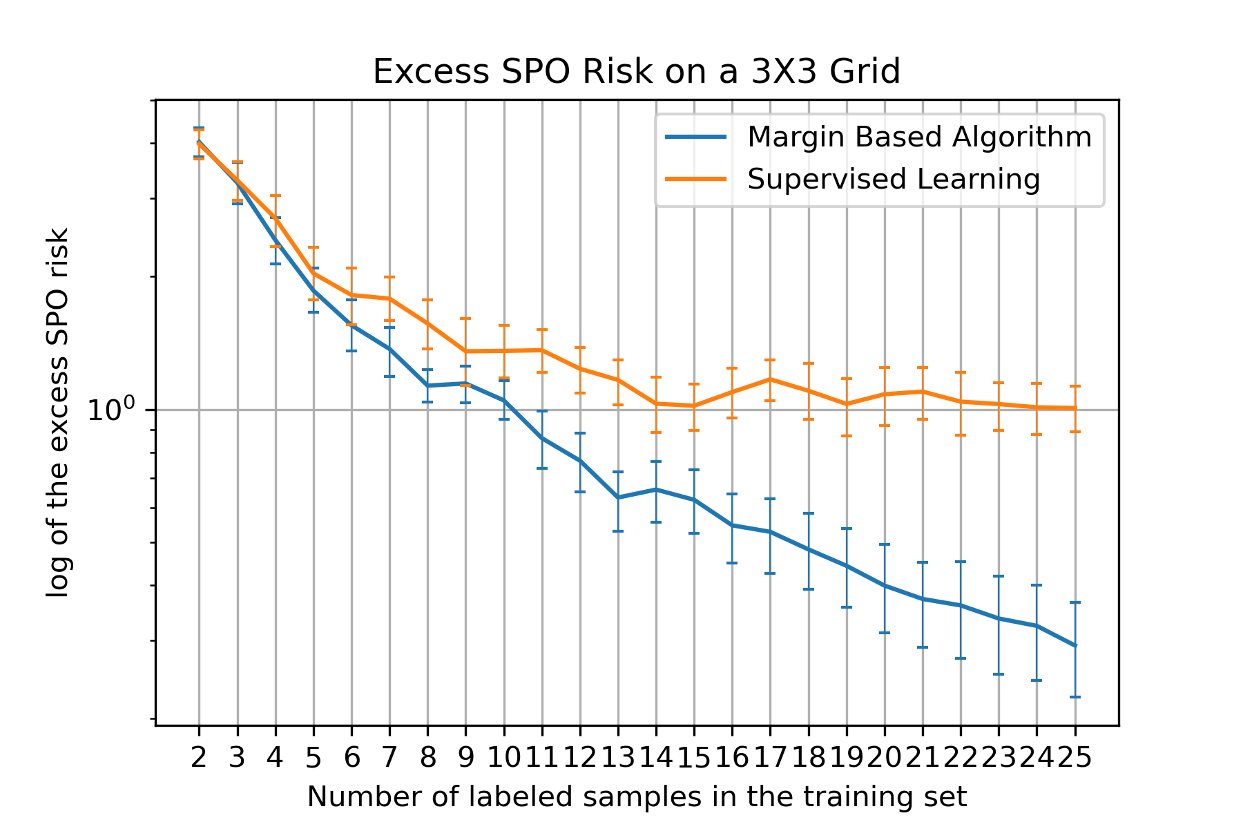
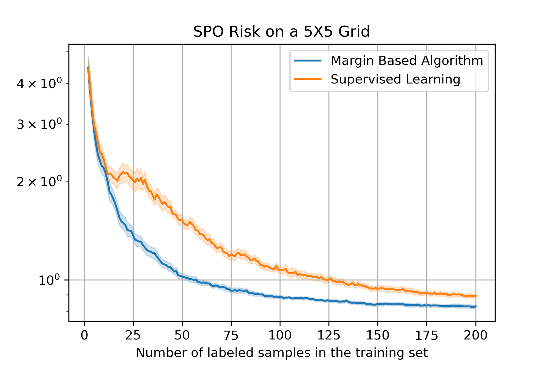
Figure 3: Risk on the test set during the training process in $3\times 3$ grid, and $5\times 5$ grid.

The margin-based algorithm has good scalability as long as the calculation of the distance to the degeneracy $\nu_{S}$ is fast, for example, in the case of relatively simple polyhedral sets. To further examine the performance of the margin-based algorithm on a larger-scale problem, we conduct a numerical experiment in a $5\times 5$ grid network in the right plot of Figure 3, again shown with an 85 % confidence interval. We see that although both algorithms converge to the same optimal SPO risk level, the margin-based algorithm has a much faster learning rate than supervised learning and can achieve a lower SPO risk even after 200 labeled samples.

In Appendix 10.1, we further examine the impacts of the scale of parameters, $r_{t}$ and $b_{t}$, on the number of labels and the SPO risk during the training process, which demonstrates the robustness of the SPO risk with respect to the scales of these parameters. In Appendix 10.2, we include more results in which we change the noise levels and variance of the features when generating the data. This verifies the advantages of our algorithms under various conditions.

6.2 Personalized Pricing Problem

In this section, we present numerical results for the personalized pricing problem. Suppose that we have three types of items, indexed by $j=1,2,3$. We have three candidate prices for these three items, which are $\$60,\$80$, and $\$90$. Therefore, in total, we have $3^{3}=27$ possible combinations of prices. Suppose that the dimension of the features of the customers is $p=6$. When a customer is selected to survey, their answers will reveal the purchase probability for all three items at all possible prices. These purchase probabilities are generated on the basis of an exponential function of the form $\mathcal{O}(e^{-p})$. We add additional price constraints between products, such that the first item has the highest price, and the third item has the lowest price. Please see the details in Appendix 10.3.

Because there are three items and three candidate prices, the dimension of the cost vector $d_{j}(p_{i})$ is $9$. Therefore, our predictor $h(x)$ is a mapping from the feature space $\mathcal{X}\subseteq\mathbb{R}^{6}$ to the label space $\mathcal{C}\subseteq[0,1]^{9}$. We assume that the predictor is a linear function, so the coefficient of $h(x)$ is a $(6+1)\times 9$ matrix, including the intercept. Unlike the shortest path problem which can be solved efficiently, the personalized pricing problem is NP-hard in general due to the binary constraints. In our case, since the dimensions of products and prices are only three, we enumerate all the possible solutions to determine the prices with the highest revenue.

The test set performance is calculated on $1000$ samples. In MBAL-SPO, we set $r_{t}=250\sqrt{[d\times\ln(t)+\ln(1/\delta)]/t}$, where $t$ is the iteration counter, $d$ is the dimension of the cost vector, which is 9, and $\delta$ is set as $10^{-7}$. According to Proposition 5.3, we set $b_{t}=0.5\times\sqrt{r_{t}}$. The scales of $r_{t}$ and $b_{t}$ are selected by the rules discussed at the end of Section 4.4. The excess SPO risks of MBAL-SPO and supervised learning on the test set as the number of acquired labels increases are shown in Figure 4. The results are from 25 simulations, and the error bars in Figure 4 represent an 85% confidence interval. Notice that the demand function is in an exponential form but our hypothesis class is linear, so the hypothesis class is misspecified. The results in Figure 4 show that MBAL-SPO achieves a smaller excess SPO risk than supervised learning even when the hypothesis class is misspecified.

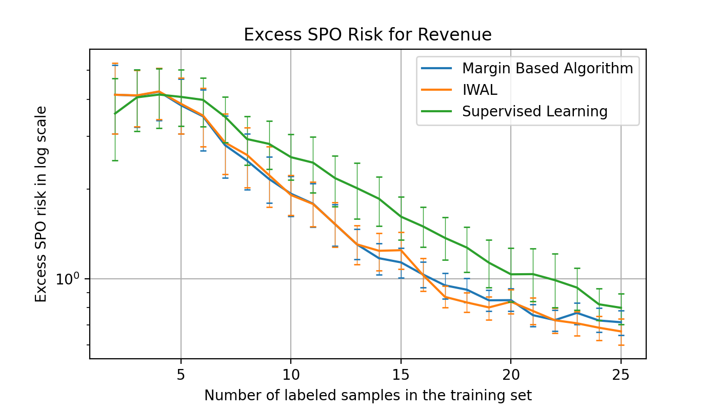
Figure 4: Excess test set risk during the training process in personalized pricing.

7 Conclusions and Future Directions

Our work develops the first active learning algorithms in the predict-then-optimize framework. We consider the SPO loss function and its tractable surrogate loss functions and provide a practical margin-based active learning algorithm (MBAL-SPO). We provide two versions of MBAL-SPO and develop excess risk guarantees for both versions. Furthermore, we provide upper bounds on the label complexity of both versions and show that the label complexity can be better than the supervised learning approach under some natural low-noise conditions. Our numerical experiments also demonstrate the practical value of our proposed algorithm. There are several intriguing future directions. Since directly minimizing the SPO loss function is challenging, one valuable direction is to design active learning algorithms in situations where we can minimize the SPO loss function approximately. While our work focuses on stream-based active learning in the predict-then-optimize framework, it is also worthwhile to consider pool-based active learning, where all feature vectors are revealed at once before training, in the future.

PG acknowledges the support of NSF AI Institute for Advances in Optimization Award 2112533.

8 Examples of $\phi$ and $\Psi$ Functions and Upper Bound for $\eta$

The existence of non-trivial $\phi$ and $\Psi$ depends on the distribution $\mathcal{D}$ and the feasible region $S$. In this appendix, we examine the case where we use the SPO+ loss as the surrogate loss function given the norm $\|\cdot\|$ as the $\ell_{2}$ norm. We first present two special cases, polyhedral and strongly convex feasible regions, for which we can characterize the function $\phi$. We then present sufficient conditions on the distribution $\mathcal{D}$ so that we can ultimately bound the label complexity. For simplicity, we use $\mathbb{P}(c|x)$ to denote the probability density function of $c$ conditional on $x$. To study the pointwise error as needed in Assumption 3.1.1, we make a recoverability assumption. Assumption 8 holds for linear hypothesis classes when the features have nonsingular covariance and for certain decision tree hypothesis classes when the density of features is bounded below by a positive constant (Hu et al. 2022). [Recoverability] There exists $\varkappa>0$ such that for all $h\in\mathcal{H}$, $h^{*}\in\mathcal{H}^{*}$, and almost all $x^{\prime}\in\mathcal{X}$, it holds that

$$\left\|h(x^{\prime})-h^{\ast}(x^{\prime})\right\|^{2}\leq\varkappa\cdot\mathbb{E}\left[\left\|h(x)-h^{\ast}(x)\right\|^{2}\right].$$

Assumption 8 provides an upper bound of the pointwise error from the bound of the expected error. It implies that the order of pointwise error is no larger than the order of the expected error.

Polyhedral feasible region.

First, we consider the case where the feasible region $S$ is a polyhedron. Let $\mathcal{P}_{\textnormal{cont, symm}}$ denote the class of joint distributions $\mathcal{D}$ such that $\mathbb{P}(\cdot|x)$ is continuous on $\mathbb{R}^{d}$ and is centrally symmetric with respect to its mean for all $x\in\mathcal{X}$. Following Theorem 2 in Liu and Grigas (2021), for given parameters $M\geq 1$ and $\alpha,\beta>0$, let $\mathcal{P}_{M,\alpha,\beta}$ denote the set of all $\mathcal{D}\in\mathcal{P}_{\textnormal{cont, symm}}$ such that for all $x\in\mathcal{X}$ and $\bar{c}=\mathbb{E}[c|x]$, there exists $\sigma\in[0,M]$ satisfying $\|\bar{c}\|_{2}\leq\beta\sigma$ and $\mathbb{P}(c|x)\geq\alpha\cdot\mathcal{N}(\bar{c},\sigma^{2}I)$ for all $c\in\mathbb{R}^{d}$. Let $D_{S}$ denote the diameter of $S$ and define a “width constant” $d_{S}$ associated with $S$ by $d_{S}:=\min_{v\in\mathbb{R}^{d}:\|v\|_{2}=1}\left\{\max_{w\in S}v^{T}w-\min_{w\in S}v^{T}w\right\}$. Notice that $d_{S}>0$ whenever $S$ has a non-empty interior.

Lemma 8.1 (Example of $\phi$)

Given $\|\cdot\|$ as the $\ell_{2}$ norm, suppose that Assumption 8 holds and the feasible region $S$ is a bounded polyhedron. Define $\Xi_{S}:=(1+\frac{2\sqrt{3}D_{S}}{d_{S}})^{1-d}$. Suppose the hypothesis class $\mathcal{H}$ is well-specified, i.e., $h^{*}(x)=\mathbb{E}[c|x]$, for all $x\in\mathcal{X}$. When the distribution $\mathcal{D}\in\mathcal{P}_{M,\alpha,\beta}$, then it holds that for almost all $x\in\mathcal{X}$,

$$R_{\textnormal{SPO+}}(h)-R_{\textnormal{SPO+}}(h^{\ast})\leq\epsilon\Rightarrow\,\|h(x)-h^{\ast}(x)\|^{2}\leq\varkappa\frac{8\sqrt{2\pi}\rho(\mathcal{\hat{C}})e^{\frac{3(1+\beta^{2})}{2}}}{\alpha\Xi_{S}}\cdot\epsilon.$$

Lemma 8.1 indicates that $\phi(\epsilon)\leq\mathcal{O}(\sqrt{\epsilon})$.

Proof 8.2

Proof of Lemma 8.1 For given $x\in\mathcal{X}$, let $\bar{c}=\mathbb{E}[c|x]$ and $\Delta=h(x)-h^{\ast}(x)$. According to Theorem 1 in Elmachtoub and Grigas (2022), it holds that

$$\mathbb{E}[\ell_{\textnormal{SPO+}}(h(x),c)-\ell_{\textnormal{SPO+}}(h^{\ast}(x),c)|x]=\mathbb{E}[(c+2\Delta)^{T}(w^{*}(c)-w^{*}(c+2\Delta))|x].$$

Without loss of generality, we assume $d_{S}>0$. Otherwise, the constant $\Xi_{S}$ will be zero and the bound will be trivial.

Define the function $\iota(\kappa):=\frac{\kappa^{2}}{M}$ for $\kappa\in[0,\frac{M}{2}]$ and $\iota(\kappa):=\kappa-\frac{M}{4}$ for $\kappa\in[\frac{M}{2},\infty)$, where $M>1$ is a scaler which is larger than $\sigma$. Let $\kappa=\|\Delta\|_{2}$ and $A\in\mathbb{R}^{d\times d}$ be an orthogonal matrix such that $A^{T}\Delta=\kappa\cdot e_{d}$ for $e_{d}=(0,\dots,0,1)^{T}$. We implement a change of basis and let the new basis be $A=(a_{1},\dots,a_{d})$. With a slight abuse of notation, we keep the notation the same after the change of basis, for example, now the vector $\Delta$ equals $\kappa\cdot e_{d}$. Rewrite $c$ as $c=(c^{\prime},\xi)$, where $c^{\prime}\in\mathbb{R}^{d-1}$ and $\xi\in\mathbb{R}$. Define $\bar{c^{\prime}}:=\mathbb{E}[c^{\prime}]$ and $\bar{\xi^{\prime}}=\mathbb{E}[\xi]$. Then by applying the results in Lemma 7 of Liu and Grigas (2021), for any $\tilde{\kappa}\in(0,\kappa]$, it holds that

$$\mathbb{E}\left[(c+2\Delta)^{T}(w^{*}(c)-w^{*}(c+2\Delta))|x\right]\geq\frac{\alpha\tilde{\kappa}\kappa e^{-\frac{3\tilde{\kappa}^{2}+3\bar{\xi}^{2}+\|\bar{c}^{\prime}\|_{2}^{2}}{2\sigma^{2}}}}{4\sqrt{2\pi\sigma^{2}}}\cdot\Xi_{S}d_{S}.$$

Let $\tilde{\kappa}=\min\{\kappa,\sigma\}$, it holds that

$$\mathbb{E}[\ell_{\textnormal{SPO+}}(h(x),c)-\ell_{\textnormal{SPO+}}(h^{\ast}(x),c)|x]\geq\frac{\alpha\Xi_{S}}{4\sqrt{2\pi}e^{\frac{3(1+\beta^{2})}{2}}}\cdot\min\left\{\frac{\kappa^{2}}{M},\kappa\right\}.$$

Define the function $\iota(\kappa):=\frac{\kappa^{2}}{M}$ for $\kappa\in[0,\frac{M}{2}]$ and $\iota(\kappa):=\kappa-\frac{M}{4}$ for $\kappa\in[\frac{M}{2},\infty)$, we have $\iota(\kappa)$ is the convex biconjugate of $\min\left\{\frac{\kappa^{2}}{M},\kappa\right\}$. By taking the expectation on $x$, it holds that

$$\mathbb{E}[\ell_{\textnormal{SPO+}}(h(x),c)-\ell_{\textnormal{SPO+}}(h^{\ast}(x),c)] \geq\frac{\alpha\Xi_{S}}{4\sqrt{2\pi}e^{\frac{3(1+\beta^{2})}{2}}}\cdot\mathbb{E}_{x}[\iota(\left\|h(x)-h^{\ast}(x)\right\|)]$$

Since $M\geq\max\{\sigma,1\}$, taking $M=2\rho(\mathcal{\hat{C}})$, we obtain that

$$R_{\textnormal{SPO+}}(h)-R_{\textnormal{SPO+}}(h^{*}) \geq\frac{\alpha\Xi_{S}}{8\sqrt{2\pi}\rho(\mathcal{\hat{C}})e^{\frac{3(1+\beta^{2})}{2}}}\cdot\mathbb{E}_{x}[\left\|h(x)-h^{\ast}(x)\right\|^{2}]$$

Then, combining the result with Assumption 8, we obtain Lemma 8.1.

Strongly-convex feasible region.

Next, we consider the case where the feasible region $S$ is a level-set of a strongly-convex and smooth function. In the spirit of Definition 4.1 in Liu and Grigas (2021), we consider two related classes of rotationally symmetric distributions with bounded conditional coefficient of variation. These distribution classes are formally defined in Definition 8.3 below, and include the multi-variate Gaussian, Laplace, and Cauchy distributions as special cases.

Definition 8.3 ($\mathcal{P}_{\beta_{1},\beta_{2}}$ distribution)

We define $\mathcal{P}_{\textnormal{rot symm}}$ as the class of joint distributions $\mathcal{D}$ with conditional rotational symmetry in the norm $\|\cdot\|$, namely for all $x\in\mathcal{X}$ and $\bar{c}=\mathbb{E}[c|x]$, there exists a function $q(\cdot):[0,\infty)\to[0,\infty)$ such that $\mathbb{P}(c|x)=q(\left\|c-\bar{c}\right\|)$. For constants $\beta_{1},\beta_{2}\in(0,1)$, define

$$\mathcal{P}_{\beta_{1},\beta_{2}}:=\left\{\mathcal{D}\in\mathcal{P}_{\textnormal{rot symm}}:\text{For any }c_{1}\in\mathbb{R}^{d},\mathbb{P}_{c|x}(0\leq c^{T}c_{1}\leq\beta_{1}\|c_{1}\|\|c\|)\geq\beta_{2}\right\}.$$

Lemma 8.4 provides a bound for the pointwise error for strongly-convex feasible regions under the class of distributions in $\mathcal{P}_{\beta_{1},\beta_{2}}$ specified in Definition 8.3.

Lemma 8.4 (Example of $\phi$)

Given $\|\cdot\|$ as the $\ell_{2}$ norm, let $f:\mathbb{R}^{d}\to\mathbb{R}$ be a $\mu_{S}$-strongly convex and $L_{S}$-smooth function for some $L_{S}\geq\mu_{S}>0$. Suppose that the feasible region $S$ is defined by $S=\{w\in\mathbb{R}^{d}:f(w)\leq r\}$ for some constant $r>f_{\min}:=\min_{w}f(w)$. Suppose that Assumption 8 holds and that the hypothesis class $\mathcal{H}$ is well-specified, i.e., $h^{*}(x)=\mathbb{E}[c|x]$, for all $x\in\mathcal{X}$. When the distribution $\mathcal{D}\in\mathcal{P}_{\beta_{1},\beta_{2}}$, then it holds that for almost all $x\in\mathcal{X}$,

$$R_{\textnormal{SPO+}}(h)-R_{\textnormal{SPO+}}(h^{\ast})\leq\epsilon\Rightarrow\,\left\|h(x)-h^{\ast}(x)\right\|^{2}\leq\frac{\varkappa\mu_{S}^{2}r^{1/2}}{2^{1/2}\beta_{2}L_{S}^{5/2}}\min\left\{\frac{2(1-\beta_{1}^{2})}{\rho(\mathcal{C},\mathcal{\hat{C}})},\frac{\sqrt{17+8\beta_{1}}-1-4\beta_{1}}{4\rho(\mathcal{C},\mathcal{\hat{C}})}\right\}^{-1}\cdot\epsilon.$$

Lemma 8.4 implies that for the strongly-convex feasible region, if the distribution $\mathcal{D}\in\mathcal{P}_{\beta_{1},\beta_{2}}$, we have $\phi(\epsilon)\leq\mathcal{O}(\sqrt{\epsilon})$. Since Theorem 4.5 also requires Assumption 4.4 holds, in Lemma 8.6 below, we provide the conditions that Assumption 4.4 holds for the SPO+ loss.

Proof 8.5

Proof of Lemma 8.4 For given $x\in\mathcal{X}$, let $\bar{c}=\mathbb{E}[c|x]$ and $\Delta=h(x)-h^{\ast}(x)$. By applying the results in Theorem C.2 of Liu and Grigas (2021), it holds that

$$\mathbb{E}\left[\ell_{\textnormal{SPO+}}(h(x),c)-\ell_{\textnormal{SPO+}}(h^{\ast}(x),c)|x\right]\geq\frac{\mu_{S}^{2}r^{1/2}}{2^{1/2}L_{S}^{5/2}}\cdot\mathbb{E}_{c|x}\left[\|c+2\Delta\|-\frac{c^{T}(c+2\Delta)}{\|c\|}\right].$$

It is easy to verify that $\|c+2\Delta\|-\frac{c^{T}(c+2\Delta)}{\|c\|}\geq 0$, for any $c\in\mathbb{R}^{d}$.

For any $\Delta$, we define a subspace $\Delta^{\perp,\beta_{1}}$ by $\Delta^{\perp,\beta_{1}}=\{c\in\mathcal{C}:0\leq c^{T}\Delta\leq\beta_{1}\|\Delta\|\|c\|\}$. By Definition 8.3, we have that $\mathbb{P}_{c|x}(c\in\Delta^{\perp,\beta_{1}})\geq\beta_{2}>0$, for any $x\in\mathcal{X}$.

Thus, we have that

$$\mathbb{E}\left[\|c+2\Delta\|-\frac{c^{T}(c+2\Delta)}{\|c\|}|x\right] \geq\mathbb{P}_{c|x}(c\in\Delta^{\perp,\beta_{1}})\mathbb{E}\left[\|c+2\Delta\|-\frac{c^{T}(c+2\Delta)}{\|c\|}\Big{|}c\in\Delta^{\perp,\beta_{1}}\right]$$

$$\geq\beta_{2}\mathbb{E}\left[\|c+2\Delta\|-\frac{c^{T}(c+2\Delta)}{\|c\|}\Big{|}c\in\Delta^{\perp,\beta_{1}}\right]$$

$$=\beta_{2}\mathbb{E}\left[\|c+2\Delta\|-\|c\|-\frac{2c^{T}\Delta}{\|c\|}\Big{|}c\in\Delta^{\perp,\beta_{1}}\right].$$

Next, we show that $\mathbb{E}\left[\|c+2\Delta\|-\|c\|-\frac{2c^{T}\Delta}{\|c\|}\Big{|}c\in\Delta^{\perp,\beta_{1}}\right]\geq\frac{1}{16\rho(\mathcal{C})}\|\Delta\|^{2}$.

Since $\|c\|\leq\rho(\mathcal{C})$, we have that

$$\|c+2\Delta\|-\|c\|-\frac{2c^{T}\Delta}{\|c\|} =\sqrt{\|c\|^{2}+4\|\Delta\|^{2}+4c^{T}\Delta}-\|c\|-\frac{2c^{T}\Delta}{\|c\|}$$

$$\geq\sqrt{\|c\|^{2}+4\|\Delta\|^{2}+4\beta_{1}\|c\|\|\Delta\|}-\|c\|-2\beta_{1}\|\Delta\|$$ (6)

$$\geq\sqrt{\rho(\mathcal{C})^{2}+4\|\Delta\|^{2}+4\beta_{1}\rho(\mathcal{C})\|\Delta\|}-\rho(\mathcal{C})-2\beta\|\Delta\|$$ (7)

Inequality (6) is because $\sqrt{\|c\|^{2}+4\|\Delta\|^{2}+4\beta_{1}\|c\|\|\Delta\|}-\|c\|-2\beta_{1}\|\Delta\|$ is a decreasing function of $\beta_{1}$. Inequality (7) is because $\sqrt{\|c\|^{2}+4\|\Delta\|^{2}+4\beta_{1}\|c\|\|\Delta\|}-\|c\|-2\beta_{1}\|\Delta\|$ is a decreasing function of $\|c\|$ when $\beta_{1}<1$.

Since $\|\Delta\|\leq 2\rho(\mathcal{C},\mathcal{\hat{C}})$, by minimizing function $f(x)=\frac{\sqrt{\rho(\mathcal{C})^{2}+2\beta_{1}\rho(\mathcal{C})x+x^{2}}-\rho(\mathcal{C})-\beta_{1}x}{x^{2}}$ over $(0,2\rho(\mathcal{C},\mathcal{\hat{C}}))$, we have that

$$\frac{\sqrt{\rho(\mathcal{C})^{2}+4\|\Delta\|^{2}+4\beta_{1}\rho(\mathcal{C})\Delta}-\rho(\mathcal{C})-2\beta_{1}\|\Delta\|}{\|\Delta\|^{2}}>\min\left\{\frac{2(1-\beta_{1}^{2})}{\rho(\mathcal{C},\mathcal{\hat{C}})},\frac{\sqrt{17+8\beta}-1-4\beta_{1}}{4\rho(\mathcal{C},\mathcal{\hat{C}})}\right\}$$

Thus, we have that $\mathbb{E}\left[\|c+2\Delta\|-\|c\|\Big{|}c\in\Delta^{\perp,\beta_{1}}\right]\geq\min\left\{\frac{2(1-\beta_{1}^{2})}{\rho(\mathcal{C},\mathcal{\hat{C}})},\frac{\sqrt{17+8\beta_{1}}-1-4\beta_{1}}{4\rho(\mathcal{C},\mathcal{\hat{C}})}\right\}\|\Delta\|^{2}$.

Thus, we conclude that for all $\mathbb{P}\in\mathcal{P}_{\beta_{1},\beta_{2}}$, it holds that

$$\left\|h(x)-h^{\ast}(x)\right\|^{2}\leq\frac{\mu_{S}^{2}r^{1/2}}{2^{1/2}\beta_{2}L_{S}^{5/2}}\min\left\{\frac{2(1-\beta_{1}^{2})}{\rho(\mathcal{C},\mathcal{\hat{C}})},\frac{\sqrt{17+8\beta_{1}}-1-4\beta_{1}}{4\rho(\mathcal{C},\mathcal{\hat{C}})}\right\}^{-1}\cdot\mathbb{E}_{c|x}\left[\ell_{\textnormal{SPO+}}(h(x),c)-\ell_{\textnormal{SPO+}}(h^{\ast}(x),c)\right].$$

Taking the expectation of both sides with $x$, we obtain that

$$\mathbb{E}[\left\|h(x)-h^{\ast}(x)\right\|^{2}]\leq\frac{\mu_{S}^{2}r^{1/2}}{2^{1/2}\beta_{2}L_{S}^{5/2}}\min\left\{\frac{2(1-\beta_{1}^{2})}{\rho(\mathcal{C},\mathcal{\hat{C}})},\frac{\sqrt{17+8\beta_{1}}-1-4\beta_{1}}{4\rho(\mathcal{C},\mathcal{\hat{C}})}\right\}^{-1}\cdot(R_{\textnormal{SPO+}}(h)-R_{\textnormal{SPO+}}(h^{*})).$$

Then, combining the result with Assumption 8, we obtain Lemma 8.4.

Lemma 8.6 (Existence of $\eta$ for $\ell_{\textnormal{SPO+}}$)

Given $\|\cdot\|$ as the $\ell_{2}$ norm, let $f:\mathbb{R}^{d}\to\mathbb{R}$ be a $\mu_{S}$-strongly convex and $L_{S}$-smooth function for some $L_{S}\geq\mu_{S}>0$. Suppose that the feasible region $S$ is defined by $S=\{w\in\mathbb{R}^{d}:f(w)\leq r\}$ for some constant $r>f_{\min}:=\min_{w}f(w)$. Suppose the hypothesis class $\mathcal{H}$ is well-specified, i.e., $h^{*}(x)=\mathbb{E}[c|x]$, for all $x\in\mathcal{X}$. Suppose distribution $\mathcal{D}\in\left\{\mathcal{D}\in\mathcal{P}_{\textnormal{rot symm}}:\mathbb{P}_{c|x}(\|c\|\geq\beta)=1,\text{for all }x\in\mathcal{X}\right\}$, for some positive $\beta>0$. Then, $\ell_{\textnormal{SPO+}}(\cdot,c)$ satisfies that for all $x\in\mathcal{X}$, $c_{1}\in\mathcal{C}$ and $h^{*}\in\mathcal{H}^{*}$,

$$|\mathbb{E}[\ell_{\textnormal{SPO+}}(c_{1},c)-\ell_{\textnormal{SPO+}}(h^{*}(x),c)|x]|\leq\frac{L_{S}^{2}\rho(\mathcal{C})\sqrt{r-f_{\mathrm{min}}}}{\sqrt{2}\mu_{S}^{1.5}}\frac{4}{\beta}\|c_{1}-h^{*}(x)\|^{2}.$$

Lemma 8.6 shows that when the feasible region is strongly convex and the hypothesis class is well-specified, and when the distribution of cost vectors is separated from the origin with probability 1, then $\eta$ in Assumption 4.4 is finite for the SPO+ loss.

Proof 8.7

Proof of Lemma 8.6 Since the hypothesis class is well-specified, we denote $h^{*}(x)$ by $\bar{c}$, given $x\in\mathcal{X}$. Then, we define $\Delta=c_{1}-\bar{c}$. According to Theorem 1 in Elmachtoub and Grigas (2022), we have that the excess SPO+ risk at $x$ for the prediction $c_{1}$ is

$$\mathbb{E}[\ell_{\textnormal{SPO+}}(\bar{c}+\Delta,c)-\ell_{\textnormal{SPO+}}(\bar{c},c)|x]=\mathbb{E}[(c+2\Delta)^{T}(w^{*}(c)-w^{*}(c+2\Delta))|x]$$

According to Lemmas 1 and 2 in Liu and Grigas (2021), we have that for any $c_{1},c_{2}\in\mathcal{C}$, it holds that

$$c_{1}^{T}(w^{*}(c_{2})-w^{*}(c_{1}))\leq\frac{L_{S}^{2}\rho(\mathcal{C})\sqrt{r-f_{\text{min}}}}{\sqrt{2}\mu_{S}^{1.5}}\left\|\frac{c_{1}}{\|c_{1}\|}-\frac{c_{2}}{\|c_{2}\|}\right\|^{2}.$$

Replacing $c_{1}$ and $c_{2}$ with $c+2\Delta$ and $c$, we obtain that

$$\mathbb{E}[\ell_{\textnormal{SPO+}}(\bar{c}+\Delta,c)-\ell_{\textnormal{SPO+}}(\bar{c},c)|x]\leq\frac{L_{S}^{2}\rho(\mathcal{C})\sqrt{r-f_{\text{min}}}}{\sqrt{2}\mu_{S}^{1.5}}\mathbb{E}\left[\left\|\frac{c}{\|c\|}-\frac{c+2\Delta}{\|c+2\Delta\|}\right\|^{2}\right].$$

Thus, to prove Lemma 8.6, it suffices to show that $\left\|\frac{c}{\|c\|}-\frac{c+2\Delta}{\|c+2\Delta\|}\right\|\leq\frac{4}{\beta}\|\Delta\|$ for any realized $c$ and any $\Delta\in\mathbb{R}^{d}$.

We consider two cases: (1) $\|2\Delta\|\geq\|c\|$, and (2) $\|2\Delta\|\leq\|c\|$.

In the first case, since $\|c\|\geq\beta$, we have that $\|2\Delta\|\geq\|c\|\geq\beta$. Since $\left\|\frac{c}{\|c\|}-\frac{c+2\Delta}{\|c+2\Delta\|}\right\|\leq 2$, we have that $\left\|\frac{c}{\|c\|}-\frac{c+2\Delta}{\|c+2\Delta\|}\right\|\leq\frac{4\|\Delta\|}{\beta}$.

In the other case, when $\|2\Delta\|\leq\|c\|$, we have

$$\left\|\frac{c}{\|c\|}-\frac{c+2\Delta}{\|c+2\Delta\|}\right\|=\sqrt{2-2\frac{c^{T}(c+2\Delta)}{\|c\|\|c+2\Delta\|}}.$$

We use $\theta\in[0,\frac{\pi}{2})$ to denote the angle between $c$ and $c+2\Delta$, then, we have $\left\|\frac{c}{\|c\|}-\frac{c+2\Delta}{\|c+2\Delta\|}\right\|=\sqrt{2-2\cos(\theta)}\leq 2\sin(\theta).$ Since $2\|\Delta\|\geq 2\|c\|\sin(\theta)$, we have that $\left\|\frac{c}{\|c\|}-\frac{c+2\Delta}{\|c+2\Delta\|}\right\|\leq\frac{2\|\Delta\|}{\|c\|}\leq\frac{2}{\beta}\|\Delta\|$. Thus, we obtain Lemma 8.6.

In conclusion of Appendix 8, it is worth noting that while our analysis in this section focused on the SPO+ loss function, similar results can be obtained for commonly used loss functions such as squared $\ell_{2}$ norm loss. For example, under some noise conditions, we can also obtain $\phi(\epsilon)\sim\sqrt{\epsilon}$ and the upper bound for $\eta$ under the squared $\ell_{2}$ norm loss.

9 Proofs

In this appendix, we provide the proofs that are omitted in the main body.

9.1 Proofs for Section 3

Proof 9.1

Proof of Lemma 3.2 Without loss of generality, assume that $\nu_{S}(c_{1})\geq\nu_{S}(c_{2})$, i.e., we have that $0\leq\|c_{1}-c_{2}\|<\nu_{S}(c_{1})$. We also claim that $\nu_{S}(c_{2})>0$. Indeed, since $\nu_{S}$ is a $1$-Lipschitz distance function, it holds that $\nu_{S}(c_{1})-\nu_{S}(c_{2})\leq\|c_{1}-c_{2}\|<\nu_{S}(c_{1})$ and hence $\nu_{S}(c_{2})>0$. As above, let $\{v_{j}:j=1,...,K\}$ be the extreme points of $S$, i.e., $S=\text{conv}(v_{1},\ldots,v_{K})$. Since $\nu_{S}(c_{1})>0$ and $\nu_{S}(c_{2})>0$, both $w^{*}(c_{1})$ and $w^{*}(c_{2})$ must be extreme points solutions, i.e., $w^{*}(c_{1})=v_{j_{1}}$ and $w^{*}(c_{1})=v_{j_{2}}$ for some indices $j_{1}$ and $j_{2}$.

We now prove the lemma by contradiction. If $w^{*}(c_{1})\not=w^{*}(c_{2})$, then by (4), the following two inequalities hold:

$$\nu_{S}(c_{1})\leq\frac{c_{1}^{T}(w^{*}(c_{2})-w^{*}(c_{1}))}{\|w^{*}(c_{2})-w^{*}(c_{1})\|_{*}},\quad\nu_{S}(c_{2})\leq\frac{c_{2}^{T}(w^{*}(c_{1})-w^{*}(c_{2}))}{\|w^{*}(c_{1})-w^{*}(c_{2})\|_{*}}.$$

We add up both sides of the above two inequalities, and get

$$\nu_{S}(c_{1})+\nu_{S}(c_{2})\leq\frac{(c_{1}-c_{2})^{T}(w^{*}(c_{2})-w^{*}(c_{1}))}{\|w^{*}(c_{2})-w^{*}(c_{1})\|_{*}}\leq\frac{\|c_{1}-c_{2}\|\|w^{*}(c_{2})-w^{*}(c_{1})\|_{*}}{\|w^{*}(c_{2})-w^{*}(c_{1})\|_{*}}=\|c_{1}-c_{2}\|,$$

where the second inequality uses Hölder’s inequality. Because $\|c_{1}-c_{2}\|<\nu_{S}(c_{1})$, we have that $\nu_{S}(c_{1})+\nu_{S}(c_{2})\leq\|c_{1}-c_{2}\|<\nu_{S}(c_{1})$. This implies that $\nu_{S}(c_{2})<0$, which contradcits that $\nu_{S}$ is a non-negative distance function. Thus, we conclude that $w^{*}(c_{1})=w^{*}(c_{2})$.

Proof 9.2

Proof of Lemma 3.4 Let $t\geq 0$ be given. First, we show that, for any given $x\in\mathcal{X}$, $\inf_{h^{*}\in\mathcal{H}^{*}}\{\nu_{S}(h^{\ast}(x))\}\geq 2b_{t}$ implies that $\nu_{S}(h_{t}(x))\geq b_{t}$. Indeed, since $\nu_{S}$ is a 1-Lipschitz distance function, we have that $|\nu_{S}(h^{*}(x))-\nu_{S}(h_{t}(x))|\leq\|h_{t}(x)-h^{*}(x)\|$ for all $h^{*}\in\mathcal{H}^{*}$. Since $\mathcal{H}^{*}_{\ell}\subseteq\mathcal{H}^{*}$ and $\text{Dist}_{\mathcal{H}^{*}_{\ell}}(h_{t})\leq b_{t}$, we have that $\text{Dist}_{\mathcal{H}^{*}}(h_{t})\leq\text{Dist}_{\mathcal{H}^{*}_{\ell}}(h_{t})\leq b_{t}$. Hence, for any $\epsilon>0$, there exists $h^{*}\in\mathcal{H}^{*}$ satisfying

$$\nu_{S}(h^{*}(x))-\nu_{S}(h_{t}(x))\leq\|h_{t}(x)-h^{*}(x)\|\leq\|h_{t}-h^{\ast}\|_{\infty}\leq b_{t}+\epsilon$$

Since the result holds for all $\epsilon>0$, we conclude that $\nu_{S}(h_{t}(x))\geq\inf_{h^{*}\in\mathcal{H}^{*}}\{\nu_{S}(h^{\ast}(x))\}-b_{t}$. Furthermore, since $\inf_{h^{*}\in\mathcal{H}^{*}}\{\nu_{S}(h^{\ast}(x))\}\geq 2b_{t}$, it holds that $\nu_{S}(h_{t}(x))\geq 2b_{t}-b_{t}=b_{t}$.

According to Algorithm 1, a label for $x_{t}$ is always acquired at iteration $t\geq 1$ if $\nu_{S}(h_{t-1}(x_{t}))<b_{t-1}$. Otherwise, if $\nu_{S}(h_{t-1}(x_{t}))\geq b_{t-1}$, then a label is acquired with probability $\tilde{p}$. Therefore, using the argument above, the label probability at iteration $t$ is

$$\mathbb{P}(\text{acquire a label for $x_{t}$}) ~{}=~{}\mathbb{P}(\nu_{S}(h_{t-1}(x_{t}))<b_{t-1})+\tilde{p}\mathbb{P}(\nu_{S}(h_{t-1}(x_{t}))\geq b_{t-1})$$

$$~{}\leq~{}\mathbb{P}(\nu_{S}(h_{t-1}(x_{t}))<b_{t-1})+\tilde{p}$$

$$~{}\leq~{}\mathbb{P}\left(\inf_{h^{*}\in\mathcal{H}^{*}}\{\nu_{S}(h^{*}(x_{t}))\}<2b_{t-1}\right)+\tilde{p}~{}\leq~{}\Psi(2b_{t-1})+\tilde{p}$$

Then, the expected number of acquired labels after $T$ total iterations is at most $\sum_{t=1}^{T}\mathbb{P}(\text{acquire a label for $x_{t}$})\leq\tilde{p}T+\sum_{t=1}^{T}\Psi(2b_{t-1})$.

9.2 Proofs for Section 4

Proof 9.3

Proof of Proposition 4.3

We use the results in Rakhlin et al. (2015a) to prove that $\ln(N_{1}(\alpha,\ell^{\mathtt{rew}}\circ\mathcal{H},T))\leq d_{\theta}\ln\left(1+\frac{2\rho(\Theta)L_{1}L_{2}}{\alpha\tilde{p}^{\mathbb{I}\{\tilde{p}>0\}}}\right)$. We use $N_{\infty}(\alpha,\ell^{\mathtt{rew}}\circ\mathcal{H},\boldsymbol{z})$ to denote the sequential covering number with respect to the $\ell_{\infty}$ norm on tree $\boldsymbol{z}$, defined analogousy to Definition 4.1. In other words, $N_{\infty}(\alpha,\ell^{\mathtt{rew}}\circ\mathcal{H},\boldsymbol{z})$ is the size of the minimal sequential cover $V$ of real-valued trees on a tree $\mathbf{z}$ of depth $T$ such that, for all $h\in\mathcal{H}$ and all paths $\boldsymbol{\sigma}\in\{\pm 1\}^{T}$, there exists a real-valued tree $\boldsymbol{v}\in V$ such that

$$\max_{t=1,...,T}\{|\boldsymbol{v}_{t}(\boldsymbol{\sigma})-\ell^{\mathtt{rew}}(h;\boldsymbol{z}_{t}(\boldsymbol{\sigma}))|\}\leq\alpha.$$

We further define the sequential covering number with respect to the $\ell_{\infty}$ norm by $N_{\infty}(\alpha,\ell^{\mathtt{rew}}\circ\mathcal{H},T):=\sup_{\boldsymbol{z}}\{N_{\infty}(\alpha,\ell^{\mathtt{rew}}\circ\mathcal{H},\boldsymbol{z})\}$.

Since the surrogate loss $\ell$ is an $L_{2}$-Lipschitz function of $h(x_{t})$ with respect to $\ell_{\infty}$ norm, and $\mathcal{H}$ is a class of functions smoothly-parameterized by $\theta\in\Theta$ with respect to the $\ell_{\infty}$ norm with parameter $L_{1}$, we have that the composition function $\ell^{\mathtt{rew}}(h;\cdot)$ is also smoothly-parameterized by $\theta\in\Theta$ with respect to the $\ell_{\infty}$ norm with parameter $\frac{L_{1}L_{2}}{\tilde{p}^{\mathbb{I}\{\tilde{p}>0\}}}$, for any given $c_{t},d^{M}_{t}$, and $q_{t}$.

We denote the i.i.d. $\ell_{\infty}$ covering number of function class $\{\ell^{\mathtt{rew}}(h;\cdot)|h\in\mathcal{H}\}$ at scale $\alpha$ by $\hat{N}_{\infty}(\alpha,\ell^{\mathtt{rew}}\circ\mathcal{H})$, which was defined in Section 4.1 after the Definition 4.1.

Since the hypothesis class is smoothly parameterized, the i.i.d. covering number, $\hat{N}_{\infty}(\alpha,\ell^{\mathtt{rew}}\circ\mathcal{H})$ is at most $\hat{N}_{\infty}(\frac{\alpha\tilde{p}^{\mathbb{I}\{\tilde{p}>0\}}}{L_{1}L_{2}},\Theta)$, for example, see Theorem 2.7.11 in Wellner et al. (2013). By Example 5.8 in Wainwright (2019), we have that $\ln(\hat{N}_{\infty}(\alpha,\Theta))\leq d_{\theta}\ln(1+\frac{2\rho(\Theta)}{\alpha})$, we have that $\ln(\hat{N}_{\infty}(\alpha,\ell^{\mathtt{rew}}\circ\mathcal{H}))\leq d_{\theta}\ln(1+\frac{2\rho(\Theta)L_{1}L_{2}}{\alpha\tilde{p}^{\mathbb{I}\{\tilde{p}>0\}}})$.

Equation (14) in Rakhlin et al. (2015a) indicates that the sequential $\ell_{\infty}$ covering number is upper bounded by the i.i.d. $\ell_{\infty}$ covering number, i.e., $\ln(N_{\infty}(\alpha,\ell^{\mathtt{rew}}\circ\mathcal{H},T))\leq\ln(\hat{N}_{\infty}(\alpha,\ell^{\mathtt{rew}}\circ\mathcal{H}))$, for all $T\geq 1$. (Intuitively, if two functions $f$ and $g$ satisfies $\|f-g\|_{\infty}\leq\alpha$, then for the values of nodes on any path, $z_{1},z_{2},...,z_{T}$, we have that $|f(z_{i})-g(z_{i})|\leq\alpha$, for $i=1,...,T$.) Thus, $\ln(N_{\infty}(\alpha,\ell^{\mathtt{rew}}\circ\mathcal{H},T))$ is at most $d_{\theta}\ln(1+\frac{2\rho(\Theta)L_{1}L_{2}}{\alpha\tilde{p}^{\mathbb{I}\{\tilde{p}>0\}}})$.

Then, by Rakhlin et al. (2015b), we have that $N_{1}(\alpha,\ell^{\mathtt{rew}}\circ\mathcal{H},T)\leq N_{\infty}(\alpha,\ell^{\mathtt{rew}}\circ\mathcal{H},T)$. Thus, $\ln(N_{1}(\alpha,\ell^{\mathtt{rew}}\circ\mathcal{H},T))$ is at most $d_{\theta}\ln(1+\frac{2\rho(\Theta)L_{1}L_{2}}{\alpha\tilde{p}^{\mathbb{I}\{\tilde{p}>0\}}})$. Thus, we have that for any fixed $\alpha>0$, $\ln(N_{1}(\alpha,\ell^{\mathtt{rew}}\circ\mathcal{H},T))\leq d_{\theta}\ln(1+\frac{2\rho(\Theta)L_{1}L_{2}}{\alpha\tilde{p}^{\mathbb{I}\{\tilde{p}>0\}}})\leq\mathcal{O}(\ln(\frac{1}{\alpha\tilde{p}^{\mathbb{I}\{\tilde{p}>0\}}}))$.

Proof 9.4

Proof of Lemma 4.8 Let $t\in\{1,\ldots,T\}$ be fixed. Since $\tilde{p}=0$, the re-weighted loss function can be written as $\ell^{\mathtt{rew}}(h;z_{t})=\ell(h(x_{t}),c_{t})d^{M}_{t}=\ell(h(x_{t}),c_{t})\mathbb{I}\{\nu_{S}(h_{t-1}(x_{t}))<b_{t-1}\}$, where $h$ refers to a generic $h\in\mathcal{H}$ throughout. Recall that $\ell(h;z_{t})$ denotes $\ell(h(x_{t}),c_{t})$ and notice that we have the following simple decomposition:

$$\ell(h;z_{t})~{}=~{}\ell(h;z_{t})(1-d^{M}_{t})+\ell(h;z_{t})d^{M}_{t},$$

Hence, by the definition of $\ell^{\text{f}}_{t}(h)$, we have

$$\mathbb{E}[\ell(h;z_{t})|\mathcal{F}_{t-1}]~{}=~{}\ell^{\text{f}}_{t}(h)+\mathbb{E}[\ell(h;z_{t})d^{M}_{t}|\mathcal{F}_{t-1}]~{}=~{}\ell^{\text{f}}_{t}(h)+\mathbb{E}[\ell^{\mathtt{rew}}(h;z_{t})|\mathcal{F}_{t-1}].$$

Since $(x_{1},c_{t}),\ldots,(x_{T},c_{T})$ are i.i.d. random variables following distribution $\mathcal{D}$, $(x_{t},c_{t})$ is independent of $\mathcal{F}_{t-1}$ and hence

$$R_{\ell}(h)=\mathbb{E}[\ell(h;z_{t})]=\mathbb{E}[\ell(h;z_{t})|\mathcal{F}_{t-1}]=\ell^{\text{f}}_{t}(h)+\mathbb{E}[\ell^{\mathtt{rew}}(h;z_{t})|\mathcal{F}_{t-1}].$$ (8)

Consider (8) applied to both $h\in\mathcal{H}$ and $h^{\ast}\in\mathcal{H_{\ell}^{\ast}}$ and averaged over $t\in\{1,\ldots,T\}$ to yield:

$$R_{\ell}(h)-R_{\ell}(h^{\ast})~{}=~{}\frac{1}{T}\sum_{t=1}^{T}\left(\ell^{\text{f}}_{t}(h)-\ell^{\text{f}}_{t}(h^{*})\right)+\frac{1}{T}\sum_{t=1}^{T}\left(\mathbb{E}[\ell^{\mathtt{rew}}(h;z_{t})|\mathcal{F}_{t-1}]-\mathbb{E}[\ell^{\mathtt{rew}}(h^{*};z_{t})|\mathcal{F}_{t-1}]\right)$$ (9)

Thus, by the definition of $Z^{\mathtt{t}}_{h}$, (9) is equivalently written as:

$$R_{\ell}(h)-R_{\ell}(h^{\ast})~{}=~{}\frac{1}{T}\sum_{t=1}^{T}\left(\ell^{\text{f}}_{t}(h)-\ell^{\text{f}}_{t}(h^{*})\right)+\frac{1}{T}\sum_{t=1}^{T}Z^{\mathtt{t}}_{h}+\frac{1}{T}\sum_{t=1}^{T}\left(\ell^{\mathtt{rew}}(h;z_{t})-\ell^{\mathtt{rew}}(h^{*};z_{t})\right).$$ (10)

Proof 9.5

Proof of Lemma 4.9 The proof is by strong induction. For the base case of $t=1$, part (a) follows since $H_{0}=\mathcal{H}$ and part (b) follows since $b_{0}\geq\sqrt{r_{0}/\eta}\geq\sqrt{\omega_{\ell}(\hat{\mathcal{C}},\mathcal{C})/\eta}$, and thus $\sup_{h\in H_{0}}\left\{\left|\ell^{\text{f}}_{1}(h)-\ell^{\text{f}}_{1}(h^{*})\right|\right\}\leq\omega_{\ell}(\mathcal{\hat{C}},\mathcal{C})\leq\eta b_{0}^{2}$.

Now, consider $t\geq 2$ and assume that parts (a) and (b) hold for all $\tilde{t}\in\{1,\ldots,t-1\}$. Namely, for all $\tilde{t}\in\{1,\ldots,t-1\}$, the following two conditions hold: (a) $h^{*}\in H_{\tilde{t}-1}$, and (b) $\sup_{h\in H_{\tilde{t}-1}}\left\{\left|\ell^{\text{f}}_{\tilde{t}}(h)-\ell^{\text{f}}_{\tilde{t}}(h^{*})\right|\right\}\leq\eta b_{\tilde{t}-1}^{2}$. Then, our goal is to show that the two claims hold for $t$.

First, we prove (a). Recall that $h^{*}$ denotes the unique minimizer of the surrogate risk $R_{\ell}$, and $h_{t-1}$ denotes the predictor from iteration $t-1$ of Algorithm 1. By Lemma 4.8, we have that

$$R_{\ell}(h_{t-1})-R_{\ell}(h^{\ast})~{}=~{}\frac{1}{t-1}\sum_{i=1}^{t-1}\left(\ell^{\mathrm{f}}_{i}(h_{t-1})-\ell^{\mathrm{f}}_{i}(h^{*})\right)+\frac{1}{t-1}\sum_{i=1}^{t-1}Z^{\mathtt{i}}_{h_{t-1}}+\frac{1}{t-1}\sum_{i=1}^{t-1}\left(\ell^{\mathtt{rew}}(h_{t-1};z_{i})-\ell^{\mathtt{rew}}(h^{*};z_{i})\right).$$

Since $R_{\ell}(h_{t-1})-R_{\ell}(h^{\ast})\geq 0$, we have that

$$\frac{1}{{t-1}}\sum_{i=1}^{t-1}(\ell^{\mathtt{rew}}(h^{*};z_{i})-\ell^{\mathtt{rew}}(h_{t-1};z_{i}))~{} \leq~{}\frac{1}{{t-1}}\sum_{i=1}^{t-1}\left(\ell^{\text{f}}_{i}(h_{t-1})-\ell^{\text{f}}_{i}(h^{*})\right)+\frac{1}{{t-1}}\sum_{i=1}^{t-1}Z^{\mathtt{i}}_{h_{t-1}}$$

$$\leq~{}\frac{1}{{t-1}}\sum_{i=1}^{t-1}\sup_{h\in H_{i-1}}\left\{\left|\ell^{\text{f}}_{i}(h)-\ell^{\text{f}}_{i}(h^{*})\right|\right\}+\frac{1}{{t-1}}\sum_{i=1}^{t-1}Z^{\mathtt{i}}_{h_{t-1}}$$

$$\leq~{}\frac{1}{{t-1}}\sum_{i=1}^{t-1}\eta b_{i-1}^{2}~{}+~{}r_{t-1},$$

where the second inequality uses $h_{t-1}\in H_{t-2}\subseteq H_{i-1}$ for $i\in\{1,\ldots,t-1\}$, and the third inequality uses assumption (b) of induction and the assumption that $r_{t}\geq\sup_{h\in\mathcal{H}}\left\{\left|\frac{1}{t}\sum_{i=1}^{t}Z^{\mathtt{i}}_{h}\right|\right\}$ for $t\geq 1$.

Recall from Algorithm 1 that the reweighted loss function at iteration $t-1$ is $\hat{\ell}^{t-1}(h)=\frac{1}{t}\sum_{(x,c)\in W_{t-1}}\ell(h(x),c)=\frac{1}{{t-1}}\sum_{i=1}^{t-1}\ell^{\mathtt{rew}}(h;z_{i})$, and $h_{t-1}$ is the corresponding minimizer over $H_{t-2}$ hence $\frac{1}{{t-1}}\sum_{i=1}^{t-1}\ell^{\mathtt{rew}}(h_{t-1};z_{i})=\hat{\ell}^{t-1,*}$. By assumption (a) of induction, we have that $h^{\ast}\in H_{t-2}$. The above chain of inequalities shows that $\hat{\ell}^{t-1}(h^{\ast})\leq\hat{\ell}^{t-1,*}+\frac{1}{{t-1}}\sum_{i=1}^{t-1}\eta b_{i-1}^{2}~{}+~{}r_{t-1}$, hence $h^{\ast}\in H_{t-1}$ by definition in Line 20 of Algorithm 1.

Next, we prove (b) for $t$. Let $h\in H_{t-1}$ be fixed. By Assumption .(2) and since $h^{*}$ is the unique minimizer in $\mathcal{H}^{*}_{\ell}$, we have that $\|h-h^{*}\|_{\infty}\leq\phi(R_{\ell}(h)-R_{\ell}^{\ast})$. By Assumption 4.4, we then have that

$$|\ell^{\text{f}}_{t}(h)-\ell^{\text{f}}_{t}(h^{*})| =\left|\mathbb{E}[\ell(h(x_{t}),c_{t})-\ell(h^{*}(x_{t}),c_{t})|d^{M}_{t}=0]\mathbb{P}(d^{M}_{t}=0|\mathcal{F}_{t-1})\right|$$

$$\leq\left|\mathbb{E}[\ell(h(x_{t}),c_{t})-\ell(h^{*}(x_{t}),c_{t})|d^{M}_{t}=0]\right|$$

$$\leq\left|\mathbb{E}[\mathbb{E}[\ell(h(x_{t}),c_{t})-\ell(h^{*}(x_{t}),c_{t})|x_{t}]|d^{M}_{t}=0]\right|$$

$$\leq\eta\mathbb{E}[\|h(x_{t})-h^{*}(x_{t})\|^{2}|d^{M}_{t}=0]$$

$$\leq\eta\left(\phi(R_{\ell}(h)-R_{\ell}^{\ast})\right)^{2}.$$ (11)

By Lemma 4.8, we have that

$$R_{\ell}(h)-R_{\ell}(h^{\ast})~{} =~{}\frac{1}{t-1}\sum_{i=1}^{t-1}\left(\ell^{\mathrm{f}}_{i}(h)-\ell^{\mathrm{f}}_{i}(h^{*})\right)+\frac{1}{t-1}\sum_{i=1}^{t-1}Z^{\mathtt{i}}_{h}+\frac{1}{t-1}\sum_{i=1}^{t-1}\left(\ell^{\mathtt{rew}}(h;z_{i})-\ell^{\mathtt{rew}}(h^{*};z_{i})\right)$$

$$\leq~{}\frac{1}{t-1}\sum_{i=1}^{t-1}\eta b_{i-1}^{2}+r_{t-1}+\frac{1}{t-1}\sum_{i=1}^{t-1}\left(\ell^{\mathtt{rew}}(h;z_{i})-\ell^{\mathtt{rew}}(h^{*};z_{i})\right)$$

$$=~{}\frac{1}{t-1}\sum_{i=1}^{t-1}\eta b_{i-1}^{2}+r_{t-1}+\hat{\ell}^{t-1}(h)-\hat{\ell}^{t-1}(h^{\ast}),$$ (12)

where the inequality follows by assumption (b) of induction since $h\in H_{t-1}\subseteq H_{i-1}$ for $i\in\{1,\ldots,t-1\}$ and the assumption that $r_{t}\geq\sup_{h\in\mathcal{H}}\left\{\left|\frac{1}{t}\sum_{i=1}^{t}Z^{\mathtt{i}}_{h}\right|\right\}$ for $t\in\{1,\ldots,T\}$, and the equality follows by the definition of the reweighted loss function in Algorithm 1. By assumption we have that $h\in H_{t-1}$ and by the proof of part (a), we have that $h^{\ast}\in H_{t-1}$. Thus, since $\hat{\ell}^{t-1,*}=\min_{h\in H_{t-2}}\hat{\ell}^{t-1}(h)$ and $H_{t-1}\subseteq H_{t-2}$, we have that

$$\hat{\ell}^{t-1,*}\leq\hat{\ell}^{t-1}(h)\leq\hat{\ell}^{t-1,*}+r_{t-1}+\frac{1}{t-1}\sum_{i=1}^{t-1}\eta b_{i-1}^{2},\text{ and }\ \hat{\ell}^{t-1,*}\leq\hat{\ell}^{t-1}(h^{\ast})\leq\hat{\ell}^{t-1,*}+r_{t-1}+\frac{1}{t-1}\sum_{i=1}^{t-1}\eta b_{i-1}^{2},$$

hence $\hat{\ell}^{t-1}(h)-\hat{\ell}^{t-1}(h^{\ast})\leq r_{t-1}+\frac{1}{t-1}\sum_{i=1}^{t-1}\eta b_{i-1}^{2}$ and by combining with (9.5) we have

$$R_{\ell}(h)-R_{\ell}(h^{\ast})~{}\leq~{}\frac{2\eta}{t-1}\sum_{i=1}^{t-1}b_{i-1}^{2}+2r_{t-1}.$$

Combining the above inequality with (9.5) yields

$$|\ell^{\text{f}}_{t}(h)-\ell^{\text{f}}_{t}(h^{*})|~{}\leq~{}\eta\left(\phi\left(\frac{2\eta}{t-1}\sum_{i=1}^{t-1}b_{i-1}^{2}+2r_{t-1}\right)\right)^{2}~{}=~{}\eta b_{t-1}^{2},$$

using the definition of $b_{t-1}$. Since $h\in H_{t-1}$ is arbitrary, the conclusion in part (b) follows.

Proof 9.6

Proof of Theorem 4.5 We provide the proof of each part separately.

Part (a).

Recall that $h^{*}$ is the unique minimizer of the surrogate risk $R_{\ell}$ under Assumption 4.4 and that $h_{T}$ is the predictor from iteration $T$ of Algorithm 1. By Lemma 4.8, we have the following decomposition:

$$R_{\ell}(h_{T})-R_{\ell}(h^{\ast})~{} =~{}\frac{1}{T}\sum_{t=1}^{T}\left(\ell^{\mathrm{f}}_{t}(h_{T})-\ell^{\mathrm{f}}_{t}(h^{*})\right)+\frac{1}{T}\sum_{t=1}^{T}Z^{\mathtt{t}}_{h_{T}}+\frac{1}{T}\sum_{t=1}^{T}\left(\ell^{\mathtt{rew}}(h_{T};z_{t})-\ell^{\mathtt{rew}}(h^{*};z_{t})\right)$$

$$=~{}\frac{1}{T}\sum_{t=1}^{T}\left(\ell^{\mathrm{f}}_{t}(h_{T})-\ell^{\mathrm{f}}_{t}(h^{*})\right)+\frac{1}{T}\sum_{t=1}^{T}Z^{\mathtt{t}}_{h_{T}}+\hat{\ell}^{T}(h_{T})-\hat{\ell}^{T}(h^{*}),$$ (13)

where we recall that the empirical re-weighted loss in Algorithm 1 is $\hat{\ell}^{T}(h):=\frac{1}{T}\sum_{(x,c)\in W_{T}}\ell(h(x),c)=\frac{1}{T}\sum_{t=1}^{T}\ell^{\mathtt{rew}}(h;z_{t})$ in this case (since $\tilde{p}=0$). We will show that $r_{t}\geq\sup_{h\in\mathcal{H}}\left\{\left|\frac{1}{t}\sum_{i=1}^{t}Z^{\mathtt{i}}_{h}\right|\right\}$ simultaneously for all $t\geq 1$ with probability at least $1-\delta$ in order to apply Lemma 4.9, again with probability at least $1-\delta$. Indeed, suppose that the conclusions of Lemma 4.9 do hold. Then, by part (a), we have $h^{*}\in H_{T-1}$ and therefore $\hat{\ell}^{T}(h_{T})\leq\hat{\ell}^{T}(h^{*})$ by the update in Line 19 of Algorithm 1. By the nested structure of the $H_{t}$ sets, we have $h_{T}\in H_{T-1}\subseteq H_{t-1}$ for all $t\in\{1,\ldots,T\}$ and therefore, by part (b), we have that $|\ell^{\mathrm{f}}_{t}(h_{T})-\ell^{\mathrm{f}}_{t}(h^{*})|\leq\eta b_{t-1}^{2}$. Thus, combining these inequalities with (9.2) yields:

$$R_{\ell}(h_{T})-R_{\ell}(h^{*})~{}\leq~{}r_{T}+\frac{1}{T}\sum_{t=0}^{T-1}\eta b_{t}^{2},$$

which is the result in part (a).

It remains to show that $r_{T}\geq\sup_{h\in\mathcal{H}}\left\{\left|\frac{1}{T}\sum_{t=1}^{T}Z^{\mathtt{t}}_{h}\right|\right\}$ simultaneously for all $T\geq 1$ with probability at least $1-\delta$. For each $T\geq 1$, we apply Proposition 4.2 and plug in both $h,h^{*}\in\mathcal{H}$. Indeed, by considering the two sequences $\{\mathbb{E}[\ell^{\mathtt{rew}}(h;z_{t})|\mathcal{F}_{t-1}]-\ell^{\mathtt{rew}}(h;z_{t})\}$ and $\{\mathbb{E}[\ell^{\mathtt{rew}}(h^{*};z_{t})|\mathcal{F}_{t-1}]-\ell^{\mathtt{rew}}(h^{*};z_{t})\}$ and their differences, we have the following bound for any $\epsilon>2\alpha>0$ with probability at least $1-2N_{1}(\alpha,\ell^{\mathtt{rew}}\circ\mathcal{H},T)\exp\left(-\frac{T(\epsilon-2\alpha)^{2}}{2\omega_{\ell}(\hat{\mathcal{C}},\mathcal{C})^{2}}\right)$:

$$\sup_{h\in\mathcal{H}}\left\{\left|\frac{1}{T}\sum_{t=1}^{T}Z^{\mathtt{t}}_{h}\right|\right\}\leq 2\epsilon.$$

Considering $\alpha=\frac{\omega_{\ell}(\hat{\mathcal{C}},\mathcal{C})}{T}$ and $\epsilon=\omega_{\ell}(\hat{\mathcal{C}},\mathcal{C})\sqrt{\frac{4\ln(2TN_{1}\left(\omega_{\ell}(\hat{\mathcal{C}},\mathcal{C})/T,\ell^{\mathtt{rew}}\circ\mathcal{H},T\right)/\delta)}{T}}+\frac{2\omega_{\ell}(\hat{\mathcal{C}},\mathcal{C})}{T}=r_{T}/2$ yields that the above bound holds with probability at least $1-\frac{\delta^{2}}{2T^{2}N_{1}\left(\omega_{\ell}(\hat{\mathcal{C}},\mathcal{C})/T,\ell^{\mathtt{rew}}\circ\mathcal{H},T\right)}>1-\frac{\delta}{2T^{2}}$. Finally, applying the union bound over all $T\geq 1$, we obtain that $r_{T}\geq\sup_{h\in\mathcal{H}}\left\{\left|\frac{1}{T}\sum_{t=1}^{T}Z^{\mathtt{t}}_{h}\right|\right\}$ simultaneously for all $T\geq 1$ with probability at least

$$1-\frac{\delta}{2}\sum_{T=1}^{\infty}\frac{1}{T^{2}}=1-\frac{\delta\pi^{2}}{12}>1-\delta.$$

Part (b).

In this part of the proof, we do not assume that $\mathcal{H}_{\ell}^{\ast}$ is a singleton as the same proof will apply later for Theorem 4.13. For any $h^{\ast}\in\mathcal{H}^{\ast}$, the excess SPO risk can be written as

$$R_{\textnormal{SPO}}(h_{T})-R_{\textnormal{SPO}}^{*}=\mathbb{E}_{(x,c)\sim\mathcal{D}}[c^{T}(w^{\ast}(h_{T}(x))-w^{\ast}(h^{*}(x)))]\leq\mathbb{E}_{(x,c)\sim\mathcal{D}}[\|c\|\|w^{\ast}(h_{T}(x))-w^{\ast}(h^{*}(x))\|_{*}].$$ (14)

We apply the conclusion of part (a), $R_{\ell}(h_{T})-R_{\ell}^{\ast}\leq r_{T}+\frac{\eta}{T}\sum_{t=0}^{T-1}b_{t}^{2}$, with probability at least $1-\delta$. Specifically, we shall provide a bound on $\Delta^{\mathrm{SPOa}}_{T}:=\mathbb{E}[R_{\textnormal{SPO}}(h_{T})-R_{\textnormal{SPO}}^{*}|R_{\ell}(h_{T})-R_{\ell}^{\ast}\leq r_{T}+\frac{\eta}{T}\sum_{t=0}^{T-1}b_{t}^{2}]$. If $b_{T}=0$, then $\phi(r_{T})=0$ and Assumption .(2) implies that $h_{T}(x)=h^{\ast}(x)$ almost everywhere and hence $\Delta^{\mathrm{SPOa}}_{T}=0$. Thus, part (b) follows immediately. Otherwise, assume that $b_{T}>0$. Recall that, by Assumption .(1), we have that $\text{Dist}_{\mathcal{H}^{*}}(h_{T})\leq\text{Dist}_{\mathcal{H}^{*}_{\ell}}(h_{T})$. Then, by combining Assumption .(2) with part (a), with probability at least $1-\delta$, for any $\epsilon>0$ there exists $h^{\ast}\in\mathcal{H}^{*}$ such that for almost every $x\in\mathcal{X}$,

$$\|h_{T}(x)-h^{\ast}(x)\|~{}\leq~{}\phi\left(r_{T}+\frac{\eta}{T}\sum_{t=0}^{T-1}b_{t}^{2}\right)+\epsilon~{}\leq~{}\phi\left(2r_{T}+\frac{2\eta}{T}\sum_{t=0}^{T-1}b_{t}^{2}\right)+\epsilon~{}=~{}b_{T}+\epsilon.$$ (15)

Since $S$ satisfies the strength property with parameter $\mu>0$, we apply part (a) of Theorem 3 of El Balghiti et al. (2022) to yield (in our notation) for any $h^{\ast}\in\mathcal{H}^{*}$ and $x\in\mathcal{X}$:

$$\|w^{\ast}(h_{T}(x))-w^{\ast}(h^{\ast}(x))\|_{\ast}~{}\leq~{}\left(\frac{1}{\mu\min\{\nu_{S}(h_{T}(x)),\nu_{S}(h^{\ast}(x))\}}\right)\|h_{T}(x)-h^{\ast}(x)\|.$$ (16)

Now, let $\gamma_{T}\geq 2b_{T}>0$ be a given parameter. For a given $x\in\mathcal{X}$ we consider two cases: (i) $\nu_{S}(h^{*}(x))>\gamma_{T}$, and (ii) $\nu_{S}(h^{*}(x))\leq\gamma_{T}$. Under case (i), we have by the 1-Lipschitzness of $\nu_{S}(\cdot)$ that $\nu_{S}(h_{T}(x))\geq\nu_{S}(h^{*}(x))-\|h_{T}(x)-h^{\ast}(x)\|>\gamma_{T}-b_{T}\geq\gamma_{T}-\gamma_{T}/2=\gamma_{T}/2$. Thus, we have that $\min\{\nu_{S}(h_{T}(x)),\nu_{S}(h^{\ast}(x))\}\geq\gamma_{T}/2$. For case (i) we will combine together (14), (15), and (16), and use the fact that $\|c\|\leq\rho(\mathcal{C})$. For case (ii), we apply the worst case bound $R_{\textnormal{SPO}}(h_{T})-R_{\textnormal{SPO}}^{*}\leq\omega_{S}(\mathcal{C})$ and note that the probability of case (ii) occurring is at most $\mathbb{P}\left(\inf_{h^{*}\in\mathcal{H}^{*}}\{\nu_{S}(h^{*}(x))\}\leq\gamma_{T}\right)=\Psi(\gamma_{T})$. Overall, we have

$$\Delta^{\mathrm{SPOa}}_{T}~{}\leq~{}\rho(\mathcal{C})\|w^{\ast}(h_{T}(x))-w^{\ast}(h^{\ast}(x))\|_{\ast}+\Psi(\gamma_{T})\omega_{S}(\mathcal{C})~{}\leq~{}\frac{2\rho(\mathcal{C})(b_{T}+\epsilon)}{\mu\gamma_{T}}+\Psi(\gamma_{T})\omega_{S}(\mathcal{C}).$$

We take $\epsilon\to 0$, and since $\gamma_{T}\geq b_{T}$ is arbitrary we take the infimum over $\gamma_{T}$ to yield part (b).

Part (c).

Again, in this part of the proof, we do not assume that $\mathcal{H}_{\ell}^{\ast}$ is a singleton as the same proof will apply later for Theorems 4.11 and 4.13. Recall that for any $h^{\ast}\in\mathcal{H}^{\ast}$, the excess SPO risk can be written as

$$R_{\textnormal{SPO}}(h_{T})-R_{\textnormal{SPO}}^{*}~{}=~{}\mathbb{E}_{(x,c)\sim\mathcal{D}}[c^{T}(w^{\ast}(h_{T}(x))-w^{\ast}(h^{*}(x)))].$$

Again, we apply part (a) with probability at least $1-\delta$. Recall that, by Assumption .(1), we have that $\text{Dist}_{\mathcal{H}^{*}}(h_{T})\leq\text{Dist}_{\mathcal{H}^{*}_{\ell}}(h_{T})$. Then, by combining Assumption .(2) with part (a), with probability at least $1-\delta$, for any $\epsilon>0$ there exists $h^{\ast}\in\mathcal{H}^{*}$ such that for almost every $x\in\mathcal{X}$,

$$\|h_{T}(x)-h^{\ast}(x)\|~{}\leq~{}\phi\left(r_{T}+\frac{\eta}{T}\sum_{t=0}^{T-1}b_{t}^{2}\right)+\epsilon~{}\leq~{}\phi\left(2r_{T}+\frac{2\eta}{T}\sum_{t=0}^{T-1}b_{t}^{2}\right)+\epsilon~{}=~{}b_{T}+\epsilon.$$ (17)

For a given $x\in\mathcal{X}$ we consider two cases: (i) $\nu_{S}(h^{*}(x))\geq 2b_{T}$, and (ii) $\nu_{S}(h^{*}(x))<2b_{T}$. Under case (i), we have that $\max\{\nu_{S}(h_{T}(x)),\nu_{S}(h^{*}(x))\}\geq 2b_{T}>b_{T}+\epsilon$ for $\epsilon<b_{T}$; thus combining Lemma 3.2 and (17) yields that $w^{\ast}(h_{T}(x))=w^{\ast}(h^{\ast}(x))$, and hence $R_{\textnormal{SPO}}(h_{T})-R_{\textnormal{SPO}}^{*}=0$, for almost every $x\in\mathcal{X}$ under case (i). For case (ii), we also apply the worst case bound $R_{\textnormal{SPO}}(h_{T})-R_{\textnormal{SPO}}^{*}\leq\omega_{S}(\mathcal{C})$ and note that the probability of case (ii) occurring is at most $\mathbb{P}\left(\inf_{h^{*}\in\mathcal{H}^{*}}\{\nu_{S}(h^{*}(x))\}<2b_{T}\right)\leq\Psi(2b_{T})$. Therefore, overall we have with probability at least $1-\delta$,

$$R_{\textnormal{SPO}}(h_{T})-R_{\textnormal{SPO}}^{*}\leq\Psi(2b_{T})\omega_{S}(\mathcal{C}).$$

Part (d).

First note that, by Assumption .(2), we have that $\mathrm{Dist}_{\mathcal{H}^{*}_{\ell}}(h_{0})\leq\phi(R_{\ell}(h_{0})-R_{\ell}^{*})\leq\phi(\omega_{\ell}(\hat{\mathcal{C}},\mathcal{C}))\leq\phi(r_{0})\leq b_{0}$. Again, we apply part (a) with probability at least $1-\delta$. Indeed, when $R_{\ell}(h_{T})-R_{\ell}^{*}\leq r_{T}+\frac{\eta}{T}\sum_{t=0}^{T-1}b_{t}^{2}$ holds, by Assumption .(2), we have that $\mathrm{Dist}_{\mathcal{H}^{*}_{\ell}}(h_{T})\leq\phi(R_{\ell}(h_{T})-R_{\ell}^{*})\leq\phi(r_{T}+\frac{\eta}{T}\sum_{t=0}^{T-1}b_{t}^{2})\leq b_{T}$. Thus, part (a) implies $\mathrm{Dist}_{\mathcal{H}^{*}_{\ell}}(h_{t})\leq b_{t}$ holds simultaneously for all $t\geq 0$ with probability at least $1-\delta$. By Lemma 3.4, since $\tilde{p}=0$, conditional on part (a), the label complexity is at most $\sum_{t=1}^{T}\Psi(2b_{t-1})$. With probability at most $\delta$, we consider the worst case label complexity $T$ and hence arrive at the overall label complexity bound of $\sum_{t=1}^{T}\Psi(2b_{t-1})+\delta T$.

Proof 9.7

Proof of Proposition 4.10 Let $\bar{h}\in\mathcal{H}$ satisfy the conditions in Assumption 4.3. We will show that $R_{\textnormal{SPO+}}(\bar{h})=0$ and therefore, since $0\leq R_{\textnormal{SPO}}(h)\leq R_{\textnormal{SPO+}}(h)$ for all $h\in\mathcal{H}$, we have that $R_{\textnormal{SPO+}}^{*}=R_{\textnormal{SPO}}^{*}=0$ and $\bar{h}$ is a minimizer for both.

Recall that for prediction $\hat{c}\in\mathbb{R}^{d}$ and realized cost vector $c\in\mathbb{R}^{d}$, the SPO+ satisfies as

$$\ell_{\textnormal{SPO+}}(\hat{c},c) :=\max_{w\in S}\left\{(c-2\hat{c})^{T}w\right\}+2\hat{c}^{T}w^{*}(c)-c^{T}w^{*}(c)$$

$$=-\min_{w\in S}\left\{(2\hat{c}-c)^{T}w\right\}+2\hat{c}^{T}w^{*}(c)-c^{T}w^{*}(c)$$

$$=(c-2\hat{c})^{T}w^{*}(2\hat{c}-c)+2\hat{c}^{T}w^{*}(c)-c^{T}w^{*}(c)$$

$$=2\hat{c}^{T}(w^{*}(c)-w^{*}(2\hat{c}-c))+c^{T}(w^{*}(2\hat{c}-c)-w^{*}(c)).$$

Under Assumption 4.3 in the polyhedral case, we have by Lemma 3.2 that $w^{*}(\bar{h}(x))=w^{*}(c)$ with probability one over $(x,c)\sim\mathcal{D}$. Similarly, we have that $\|(2\bar{h}(x)-c)-\bar{h}(x)\|=\|\bar{h}(x)-c\|\leq\varrho\nu_{S}(\bar{h}(x))<\nu_{S}(\bar{h}(x))$, and hence $w^{*}(2\bar{h}(x)-c)=w^{*}(\bar{h}(x))=w^{*}(c)$, with probability one over $(x,c)\sim\mathcal{D}$. Therefore, we have that $R_{\textnormal{SPO+}}(\bar{h})=\mathbb{E}_{(x,c)\sim\mathcal{D}}[\ell_{\textnormal{SPO+}}(\bar{h}(x),c)]=0$ by the above expression for $\ell_{\textnormal{SPO+}}(\hat{c},c)$.

Proof 9.8

Proof of Theorem 4.11 We provide the proof of part (a), as the proofs of parts (b) and (c) are completely analogous to Theorem 4.5.

Recall that $(x_{1},c_{1}),(x_{2},c_{2}),\ldots$ is the sequence of features and corresponding cost vectors of Algorithm 1. It is assumed that this sequence is an i.i.d. sequence from the distribution $\mathcal{D}$ and note that $c_{t}$ is only observed when we do not reject $x_{t}$, i.e., when $d_{t}^{M}=\mathbb{I}(\nu_{S}(h_{t-1}(x_{t}))<b_{t-1})=1$. In a slight abuse of notation, in this proof only, let us define $Z^{\mathtt{t}}_{h}:=\mathbb{E}[\ell_{\textnormal{SPO+}}(h(x_{t}),c_{t})]-\ell_{\textnormal{SPO+}}(h(x_{t}),c_{t})=R_{\textnormal{SPO+}}(h)-\ell_{\textnormal{SPO+}}(h(x_{t}),c_{t})$. Following the template of Lemma 4.9, the main idea of the proof is to show that, when $r_{t}\geq\sup_{h\in\mathcal{H}}\left\{\left|\frac{1}{t}\sum_{i=1}^{t}Z^{\mathtt{i}}_{h}\right|\right\}$ for all $t\geq 1$, we have that:

$$(A)\ \max_{t\in\{1,\ldots,T\}}\left\{\ell_{\textnormal{SPO+}}(h_{T}(x_{t}),c_{t})\right\}=0\ \text{ with probability 1 for all }T\geq 1.$$

In other words, $h_{T}$ achieves zero SPO+ loss across the entire sequence $(x_{1},c_{1}),\ldots,(x_{T},c_{T})$. In fact, we show a strong result, which is that (A) holds for all minimizers of the empirical reweighted loss at iteration $T$. The proof of this is by strong induction, and we defer it to the end.

Notice that $\max_{t\in\{1,\ldots,T\}}\left\{\ell_{\textnormal{SPO+}}(h_{T}(x_{t}),c_{t})\right\}=0$ implies, of course, that $h_{T}$ achieves zero (and hence minimizes) empirical risk $\frac{1}{T}\sum_{t=1}^{T}\ell_{\textnormal{SPO+}}(h(x_{t}),c_{t})$. Thus, using $r_{t}\geq\sup_{h\in\mathcal{H}}\left\{\left|\frac{1}{t}\sum_{i=1}^{t}Z^{\mathtt{i}}_{h}\right|\right\}$ for all $t\geq 1$, we have that

$$R_{\textnormal{SPO+}}(h_{T})=R_{\textnormal{SPO+}}(h_{T})-\frac{1}{T}\sum_{t=1}^{T}\ell_{\textnormal{SPO+}}(h_{T}(x_{t}),c_{t})=\frac{1}{T}\sum_{t=1}^{T}Z^{\mathtt{t}}_{h_{T}}\leq r_{T},$$

which is the result of part (a). To control the probability that $r_{t}\geq\sup_{h\in\mathcal{H}}\left\{\left|\frac{1}{t}\sum_{i=1}^{t}Z^{\mathtt{i}}_{h}\right|\right\}$, we now consider the i.i.d. covering number instead of the sequential covering number. As pointed out by Kuznetsov and Mohri (2015), in the i.i.d. case, for $T\geq 1$ and for any $\epsilon>2\alpha>0$, we have a similar convergence result as Proposition 4.2 as follows:

$$\mathbb{P}\left(\sup_{h\in\mathcal{H}}\left\{\left|R_{\textnormal{SPO+}}(h)-\frac{1}{T}\sum_{t=1}^{T}\ell_{\textnormal{SPO+}}(h(x_{t}),c_{t})\right|\right\}\geq\epsilon\right)\leq 2\hat{N_{1}}(\alpha,\ell_{\textnormal{SPO+}}\circ\mathcal{H})\exp\left\{-\frac{T(\epsilon-2\alpha)^{2}}{2\omega_{\ell}(\hat{\mathcal{C}},\mathcal{C})^{2}}\right\}.$$

Considering $\alpha=\frac{\omega_{\ell}(\hat{\mathcal{C}},\mathcal{C})}{T}$ and $\epsilon=\omega_{\ell}(\hat{\mathcal{C}},\mathcal{C})\sqrt{\frac{4\ln(2T\hat{N_{1}}(\alpha,\ell_{\textnormal{SPO+}}\circ\mathcal{H})/\delta)}{T}}+\frac{2\omega_{\ell}(\hat{\mathcal{C}},\mathcal{C})}{T}=r_{T}$ and following the same reasoning as in the proof of Theorem 4.5 yields that $r_{T}\geq\sup_{h\in\mathcal{H}}\left\{\left|\frac{1}{T}\sum_{t=1}^{T}Z^{\mathtt{t}}_{h}\right|\right\}$ simultaneously for all $T\geq 1$ with probability at least $1-\delta$.

Proof of Claim (A).

It remains to show that (A) holds for all $T\geq 1$, which we prove by strong induction. In fact, we prove a stronger variant of (A) as follows. Recall that $\hat{\ell}^{T}(h)=\frac{1}{T}\sum_{(x,c)\in W_{T}}\ell_{\textnormal{SPO+}}(h(x),c)$ is the empirical reweighed loss at iteration $T$. Define $H_{T}^{0}:=\{h\in\mathcal{H}:\hat{\ell}^{T}(h)=0\}=\{h\in\mathcal{H}:\ell_{\textnormal{SPO+}}(h(x),c)=0\text{ for all }(x,c)\in W_{T}\}$. The set $H_{T}^{0}$ is exactly the set of minimizers of $\hat{\ell}^{T}(h)$, with probability 1, since Proposition 4.10 (in particular $R_{\textnormal{SPO+}}^{*}=0$) implies that $\hat{\ell}^{T}(h^{*})=0$ with probability 1. Hence, $h_{T}\in H_{T}^{0}$ with probability 1.

Let us also define $\bar{H}_{T}^{0}:=\{h\in\mathcal{H}:\ell_{\textnormal{SPO+}}(h(x_{t}),c_{t})=0\text{ for all }t=1,\ldots,T\}$. Clearly, $\bar{H}_{T}^{0}\subseteq H_{T}^{0}$ for all $T\geq 1$. Note also that both collections of sets are nested, i.e., $H_{T}^{0}\subseteq H_{T-1}^{0}\subseteq\cdots H_{1}^{0}\subseteq\mathcal{H}$ and $\bar{H}_{T}^{0}\subseteq\bar{H}_{T-1}^{0}\subseteq\cdots\bar{H}_{1}^{0}\subseteq\mathcal{H}$. Now, we will use strong induction to prove, when $r_{t}\geq\sup_{h\in\mathcal{H}}\left\{\left|\frac{1}{t}\sum_{i=1}^{t}Z^{\mathtt{i}}_{h}\right|\right\}$ for all $t\geq 1$, we have that:

$$(\bar{A})\ \ H_{T}^{0}=\bar{H}_{T}^{0}\ \text{ with probability 1 for all }T\geq 1.$$

Note that ($\bar{A}$) implies (A) since $h_{T}\in H_{T}^{0}$ with probability 1.

To prove the base case $T=1$, we observe that $b_{0}\geq\rho(\mathcal{\hat{C}})$, and thus, $\nu_{S}(h(x_{1}))\leq\|h(x_{1})\|\leq\rho(\mathcal{\hat{C}})\leq b_{0}$ for any $h\in\mathcal{H}$ and any $x_{1}\in\mathcal{X}$. Thus, we have that $d_{1}^{M}=1$ with probability 1 and the sample $(x_{1},c_{1})$ is added to working set $W_{1}$. By definition of $H_{1}^{0}$, for $h\in H_{1}^{0}$ we have that $\ell_{\textnormal{SPO+}}(h(x_{1}),c_{1})=0$. Hence, $h\in\bar{H}_{1}^{0}$ and so we have proven that $H_{1}^{0}\subseteq\bar{H}_{1}^{0}$.

Now, consider $T\geq 2$ and assume that ($\bar{A}$) holds for all $\tilde{T}\in\{1,\ldots,T-1\}$. We need to show that $H_{T}^{0}\subseteq\bar{H}_{T}^{0}$, so let $h\in H_{T}^{0}$ be given. By the induction hypothesis, we have that $h\in H_{T-1}^{0}=\bar{H}_{T-1}^{0}$, and therefore we have $\ell_{\textnormal{SPO+}}(h(x_{t}),c_{t})=0$ for all $t\in\{1,\ldots,T-1\}$. Thus, to show that $h\in\bar{H}_{T}^{0}$, it suffices to show that $\ell_{\textnormal{SPO+}}(h(x_{T}),c_{T})=0$ with probability 1.

There are two cases to consider. First, if $d_{T}^{M}=1$, then the sample $(x_{T},c_{T})$ is added to working set $W_{T}$ and thus, by definition of $H_{T}^{0}$, for $h\in H_{T}^{0}$ we have that $\ell_{\textnormal{SPO+}}(h(x_{T}),c_{T})=0$. Hence, $h\in\bar{H}_{T}^{0}$ and so we have proven that $H_{T}^{0}\subseteq\bar{H}_{T}^{0}$.

Second, let us consider the case where $d_{T}^{M}=0$ so we do not acquire the label $c_{T}$. In this case, we have that $W_{T}=W_{T-1}$, $H_{T}^{0}=H_{T-1}^{0}$, and, by the rejection criterion, $\nu_{S}(h_{T-1}(x_{T}))\geq b_{T-1}$. For the given $h\in H_{T}^{0}$, to show that $\ell_{\textnormal{SPO+}}(h(x_{T}),c_{T})=0$ with probability 1 recall from the proof of Proposition 4.10 that is suffices to show that $w^{*}(2h(x_{T})-c_{T})=w^{*}(c_{T})$ with probability 1 over $c_{T}$ drawn from the conditional distribution given $x_{T}$.

To prove this, first note that

$$R_{\textnormal{SPO+}}(h)=R_{\textnormal{SPO+}}(h)-\frac{1}{T-1}\sum_{t=1}^{T-1}\ell_{\textnormal{SPO+}}(h(x_{t}),c_{t})=\frac{1}{T-1}\sum_{t=1}^{T-1}Z^{\mathtt{t}}_{h}\leq r_{T-1},$$

where the first equality uses that $h\in H^{0}_{T}=H^{0}_{T-1}=\bar{H}^{0}_{T-1}$ and the inequality uses the assumption that $r_{t}\geq\sup_{h\in\mathcal{H}}\left\{\left|\frac{1}{t}\sum_{i=1}^{t}Z^{\mathtt{i}}_{h}\right|\right\}$ for all $t\geq 1$. By similar reasoning, we have that $h_{T-1}\in H^{0}_{T-1}=\bar{H}^{0}_{T-1}$ satisfies $R_{\textnormal{SPO+}}(h_{T-1})\leq r_{T-1}$. Let $\epsilon>0$ be fixed. Now, by Assumption 3.1.1 and Proposition 4.10, there exists $h^{*}_{0}\in\mathcal{H}^{*}_{\text{SPO+}}$ such that

$$\|h(x_{T})-h^{*}_{0}(x_{T})\|\leq\phi(R_{\textnormal{SPO+}}(h))+\epsilon\leq\phi(r_{T-1})+\epsilon\leq\frac{\tau(1-\varrho)}{\tau(1-\varrho)+2}b_{T-1}+\epsilon,$$

and there exists $h^{*}_{1}\in\mathcal{H}^{*}_{\text{SPO+}}$ such that

$$\|h_{T-1}(x_{T})-h^{*}_{1}(x_{T})\|\leq\phi(R_{\textnormal{SPO+}}(h_{T-1}))+\epsilon\leq\phi(r_{T-1})+\epsilon\leq\frac{\tau(1-\varrho)}{\tau(1-\varrho)+2}b_{T-1}+\epsilon,$$

where we have used $b_{T-1}=(1+\frac{2}{\tau(1-\rho)})\phi(r_{T-1})$ in both inequalities above. Since both $h^{*}_{0},h^{*}_{1}\in\mathcal{H}^{*}_{\text{SPO+}}$, according to the proof of Proposition 4.10, we have that $w^{*}(2h^{*}_{0}(x_{T})-c_{T})=w^{*}(c_{T})=w^{*}(2h^{*}_{1}(x_{T})-c_{T})$ with probability 1. By the rejection criterion, $\nu_{S}(h_{T-1}(x_{T}))\geq b_{T-1}$, and the 1-Lipschitzness of $\nu_{S}$, we have

$$\nu_{S}(h^{*}_{1}(x_{T})) =\nu_{S}(h^{*}_{1}(x_{T})-h_{T-1}(x_{T})+h_{T-1}(x_{T}))\geq\nu_{S}(h_{T-1}(x_{T}))-\|h^{*}_{1}(x_{T})-h_{T-1}(x_{T})\|-\epsilon$$

$$\geq b_{T-1}-\frac{\tau(1-\varrho)}{\tau(1-\varrho)+2}b_{T-1}-\epsilon=\frac{2}{\tau(1-\varrho)+2}b_{T-1}-\epsilon.$$

By the second part of Assumption 4.3, we have that

$$\nu_{S}(h^{*}_{0}(x_{T}))\geq\tau\left(\sup_{h^{\prime}\in\mathcal{H}_{\mathrm{SPO}+}^{\ast}}\{\nu_{S}(h^{\prime}(x_{T}))\}\right)\geq\tau\nu_{S}(h^{*}_{1}(x_{T}))\geq\frac{2\tau}{\tau(1-\varrho)+2}b_{T-1}-\epsilon\tau.$$

By viewing $2h(x_{T})-c_{T}$ and $2h^{*}_{0}(x_{T})-c_{T}$ as $c_{1}$ and $c_{2}$ in Lemma 3.2, we have

$$\|(2h(x_{T})-c_{T})-(2h^{*}_{0}(x_{T})-c_{T})\|=2\|h(x_{T})-h^{*}_{0}(x_{T})\|\leq\frac{2\tau(1-\varrho)}{\tau(1-\varrho)+2}b_{T-1}+2\epsilon.$$

By the 1-Lipschitzness of $\nu_{S}$ and the first part of Assumption 4.3, we have

$$\nu_{S}(2h^{*}_{0}(x_{T})-c_{T}) \geq\nu_{S}(h^{*}_{0}(x_{T}))-\|h^{*}_{0}(x_{T})-c_{T}\|\geq(1-\varrho)\nu_{S}(h^{*}_{0}(x_{T}))$$

$$\geq(1-\varrho)\left(\frac{2\tau}{\tau(1-\varrho)+2}b_{T-1}-\epsilon\tau\right)=\frac{2\tau(1-\varrho)}{\tau(1-\varrho)+2}b_{T-1}-(1-\varrho)\epsilon\tau.$$

By taking $\epsilon\to 0$ and considering an appropriate convergent subsequence in the compact set $\mathcal{H}^{*}_{\text{SPO+}}$, the two inequalities above are satisfied for some $\bar{h}^{*}_{0}\in\mathcal{H}^{*}_{\text{SPO+}}$ with $\epsilon=0$. In particular, this implies that the conditions in Lemma 3.2 are satisfied and we have that $w^{*}(2h(x_{T})-c_{T})=w^{*}(2\bar{h}^{*}_{0}(x_{T})-c_{T})=w^{*}(c_{T})$ with probability 1. Hence, we have shown that $\ell_{\textnormal{SPO+}}(h(x_{T}),c_{T})=0$ with probability 1, and so we have proven that $H_{T}^{0}\subseteq\bar{H}_{T}^{0}$.

Proof 9.9

Proof of Theorem 4.13

We provide the proof of part (a), as the proofs of parts (b), (c), and (d) are completely analogous to Theorem 4.5.

Let us now prove part (a). When $T=0$, part (a) holds by the definition of $r_{0}\geq\omega_{\ell}(\hat{\mathcal{C}},\mathcal{C})$. Otherwise, let $T\geq 1$ be given. For any $t\in\{1,\ldots,T\}$, recall that the re-weighted loss function at iteration $t$ is in this case given by $\ell^{\mathtt{rew}}(h;z_{t}):=d^{M}_{t}\ell(h(x_{t}),c_{t})+(1-d^{M}_{t})(q_{t}/\tilde{p})\ell(h(x_{t}),c_{t})$. Since $\tilde{p}>0$, and $q_{t}$ is a random variable that independent of $x_{t},c_{t}$, and $d^{M}_{t}$, we condition on the two possible values of $q_{t}\in\{0,1\}$ and obtain the following decomposition:

$$\mathbb{E}[\ell^{\mathtt{rew}}(h;z_{t})|\mathcal{F}_{t-1}] =\mathbb{E}[\ell(h(x_{t}),c_{t})d^{M}_{t}|\mathcal{F}_{t-1}]+\mathbb{E}[\ell(h(x_{t}),c_{t})(1-d^{M}_{t})|\mathcal{F}_{t-1}]$$

$$=\mathbb{E}[\ell(h(x_{t}),c_{t})|\mathcal{F}_{t-1}]=\mathbb{E}[\ell(h(x_{t}),c_{t})]=R_{\ell}(h),$$

where we have also used that $(x_{t},c_{t})$ is independent of $\mathcal{F}_{t-1}$. In other words, the conditional expectation of re-weighted surrogate loss at iteration $t$ equals the surrogate risk. Consider the above applied to both $h\in\mathcal{H}$ and $h^{\ast}\in\mathcal{H_{\ell}^{\ast}}$ and averaged over $t\in\{1,\ldots,T\}$ to yield:

$$R_{\ell}(h)-R_{\ell}(h^{\ast})~{}=~{}\frac{1}{T}\sum_{t=1}^{T}\left(\mathbb{E}[\ell^{\mathtt{rew}}(h;z_{t})|\mathcal{F}_{t-1}]-\mathbb{E}[\ell^{\mathtt{rew}}(h^{\ast};z_{t})|\mathcal{F}_{t-1}]\right)$$ (18)

As before, we denote the discrepancy between the expectation and the true excess re-weighted loss of predictor $h$ at time $t$ by $Z^{\mathtt{t}}_{h}$, i.e., $Z^{\mathtt{t}}_{h}:=\mathbb{E}[\ell^{\mathtt{rew}}(h;z_{t})-\ell^{\mathtt{rew}}(h^{*};z_{t})|\mathcal{F}_{t-1}]-(\ell^{\mathtt{rew}}(h;z_{t})-\ell^{\mathtt{rew}}(h^{*};z_{t}))$. Recall that the empirical re-weighted loss in Algorithm 1 is $\hat{\ell}^{T}(h)=\frac{1}{T}\left(\sum_{(x,c)\in W_{T}}\ell(h(x),c)+\frac{1}{\tilde{p}}\sum_{(x,c)\in\tilde{W}_{T}}\ell(h(x),c)\right)=\frac{1}{T}\sum_{t=1}^{T}\ell^{\mathtt{rew}}(h;z_{t})$. Thus, (18) is equivalently written as:

$$R_{\ell}(h)-R_{\ell}(h^{\ast})~{}=~{}\frac{1}{T}\sum_{t=1}^{T}Z^{\mathtt{t}}_{h}+\frac{1}{T}\sum_{t=1}^{T}\left(\ell^{\mathtt{rew}}(h;z_{t})-\ell^{\mathtt{rew}}(h^{*};z_{t})\right),$$ (19)

for any $h\in\mathcal{H}$. To bound the term $\frac{1}{T}\sum_{t=1}^{T}Z^{\mathtt{t}}_{h}$, we apply Proposition 4.2 twice to both $h$ and $h^{\ast}$, with $\alpha\leftarrow\frac{\omega_{\ell}(\mathcal{\hat{C}},\mathcal{C})}{T}$ and $\epsilon\leftarrow\frac{\omega_{\ell}(\hat{\mathcal{C}},\mathcal{C})}{\tilde{p}}\sqrt{\frac{4\ln(2TN_{1}(\alpha,\ell^{\mathtt{rew}}\circ\mathcal{H},T)/\delta)}{T}}+2\alpha$. Then, by considering their differences using the union bound we have that

$$\sup_{h\in\mathcal{H}}\left|\frac{1}{T}\sum_{t=1}^{T}Z^{\mathtt{t}}_{h}\right|~{}\leq~{}2\epsilon=r_{T},$$

with probability at least $1-\frac{\delta}{2T^{2}}$. Since $h_{T}$ is the minimizer of the empirical re-weighted loss $\hat{\ell}^{T}(h)$ over $\mathcal{H}$, we have that $\ell^{\mathtt{rew}}(h_{T};z_{t})-\ell^{\mathtt{rew}}(h^{*};z_{t})\leq 0$ in (19) and we obtain that $R_{\ell}(h)-R_{\ell}(h^{\ast})\leq r_{T}$ with probability at least $1-\frac{\delta}{2T^{2}}$. Finally, applying the union bound over all $T\geq 1$, we obtain that $R_{\ell}(h)-R_{\ell}(h^{\ast})\leq r_{T}$ simultaneously for all $T\geq 1$ with probability at least $1-\delta$, which is the result of part (a).

9.3 Proofs for Section 5

Proof 9.10

Proof of Proposition 5.1

Since $\phi(\epsilon)=C_{\phi}\sqrt{\epsilon}$, and $C_{\phi}\in(0,\frac{1}{36L^{2}})$, we set $\bar{C}=\sqrt{\frac{r_{1}}{5L}}$. We use induction to prove that $b_{T}\leq\bar{C}/T^{-1/4}$, for all $T$. For simplicity, we ignore the log term when analyzing the order, and assume that $r_{t}\leq\frac{r_{1}}{\sqrt{t}}$.

We assume $b_{t}\leq\bar{C}/t^{-1/4}$, for $1\leq t\leq T-1$.

Then, since $b_{t}=2\phi(2r_{t}+\frac{2L}{t}\sum_{i=0}^{t-1}b_{i}^{2})$, we have that when $t=T$,

$$b_{t} =2C_{\phi}\sqrt{r_{t}+\frac{2L}{t}\sum_{i=0}^{t-1}b_{i}^{2}}$$

$$\leq 2C_{\phi}\sqrt{\frac{r_{1}}{\sqrt{t}}+\frac{2L}{t}\sum_{i=0}^{t-1}b_{i}^{2}}$$

$$\leq 2C_{\phi}\sqrt{\frac{r_{1}}{\sqrt{t}}+\frac{2L}{t}\sum_{i=0}^{t-1}\frac{\bar{C}^{2}}{\sqrt{i}}}$$

$$\leq 2C_{\phi}\sqrt{\frac{r_{1}}{\sqrt{t}}+\frac{4L}{t}\bar{C}\sqrt{t}}.$$

The first inequality is by $r_{t}\leq\frac{r_{1}}{\sqrt{t}}$. The last inequality is from the fact that $\frac{1}{t}\sum_{i=0}^{t-1}i^{-1/2}\leq 2\sqrt{t}$.

Then, we plug in the value of $\bar{C}$, we have that $b_{t}\leq\bar{C}/t^{-1/4}$, when $t=T$. Thus, $R_{\textnormal{SPO+}}(h_{T})-R_{\textnormal{SPO+}}^{*}\leq\mathcal{\tilde{O}}(T^{-1/4})$. Consequently, for the polyhedral case, $R_{\textnormal{SPO}}(h_{T})-R_{\textnormal{SPO}}^{*}\leq 2\Psi(2b_{T})\omega_{S}(\mathcal{C})\leq\mathcal{\tilde{O}}(T^{-\kappa/4})$. For the strongly-convex feasible region, we set $\gamma_{T}=b$, and then we can obtain the same order $\mathcal{\tilde{O}}(T^{-\kappa/4})$ for the excess SPO risk.

Next, we consider the bound for the label complexity. We set $\delta$ as a very small number, for example, $\delta\leq\mathcal{\tilde{O}}(1/T^{3})$, so we can ignore the last term in the label complexity in part (d). Then, we have that $\mathbb{E}[n_{t}]\leq\mathcal{\tilde{O}}(2\sum_{t=1}^{T}\Psi(2b_{t}))$. Because $b_{t}\leq\mathcal{\tilde{O}}(T^{-\kappa/2})$, we have that $\sum_{t=1}^{T}\Psi(2b_{t})\leq\mathcal{\tilde{O}}(T^{1-\kappa/2})$. Then, we can obtain the label complexity in Proposition 5.1 depending on the value of $\kappa$.

Proof 9.11

Proof of Proposition 5.3 We first consider the label complexity. By the part (d) in Theorem 4.13, the total label complexity $\mathbb{E}[n_{t}]$ is at most

$$\tilde{p}T+2\sum_{t=1}^{T}\Psi(2b_{t}) =\tilde{p}T+\sum_{t=1}^{T}2\Psi\left(2\phi\left(\frac{1}{\tilde{p}}\sqrt{2\ln(t/\delta)/t}\right)\right)$$

$$\leq\tilde{p}T+\sum_{t=1}^{T}C^{\prime}\cdot\left(\frac{1}{\tilde{p}}\right)^{\frac{\kappa}{2}}\left(\ln(t/\delta)/t\right)^{\kappa/4}$$

$$\leq\mathcal{\tilde{O}}\left(\tilde{p}T+\left(\frac{1}{\tilde{p}}\right)^{\frac{\kappa}{2}}(T\ln T)^{1-\kappa/4}\right).$$

The first inequality is because of assumptions 8 and 5.1. The second inequality is because of the integration. To minimize the order of $T$, we set $\tilde{p}=T^{-\frac{k}{2(k+2)}}$. Then, the label complexity $\mathbb{E}[n_{t}]$ is at most $\mathcal{\tilde{O}}\left(T^{1-\frac{k}{2(k+2)}}\right)$ for $\kappa>0$.

Next, since $r_{T}\leq\mathcal{\tilde{O}}(\frac{1}{\sqrt{T}\tilde{p}})=\mathcal{\tilde{O}}(T^{-\frac{1}{\kappa+2}})$, we obtain the risk bounds for the surrogate loss. Since $\phi$ is a square root function. The SPO risk is at most $2\Psi(2\phi(r_{T}))\leq\mathcal{\tilde{O}}(T^{-\frac{\kappa}{2(\kappa+2)}})$.

Proof 9.12

Proof of Proposition 5.5 The reason why the excess surrogate risk in Proposition 5.3 is larger than $\mathcal{\tilde{O}}(T^{-1/2})$ is because $r_{T}\leq\mathcal{\tilde{O}}(\frac{1}{\tilde{p}\sqrt{T}})$. Indeed, when $\tilde{p}\leftarrow T^{-\frac{\kappa}{2(\kappa+2)}}$, then $r_{T}\leq\mathcal{\tilde{O}}\left(T^{\left(\frac{\kappa}{2(\kappa+2)}-\frac{1}{2}\right)}\right)$, which is larger than $\mathcal{\tilde{O}}(T^{-1/2})$. Moreover, the dependence on $\tilde{p}$ comes from the bound on the re-weighted loss, since the re-weighted loss is upper-bounded by $\frac{\omega_{\ell}(\hat{\mathcal{C}},\mathcal{C})}{\tilde{p}}$. When $T\rightarrow\infty$, $\tilde{p}\rightarrow 0$, and thus, the re-weighted loss tends to infinity.

Given the output predictor $h_{T}$ at iteration $T$, recall that $Z^{\mathtt{t}}_{h_{T}}:=\mathbb{E}[\ell^{\mathtt{rew}}(h_{T};z_{t})-\ell^{\mathtt{rew}}(h^{*};z_{t})|\mathcal{F}_{t-1}]-(\ell^{\mathtt{rew}}(h_{T};z_{t})-\ell^{\mathtt{rew}}(h^{*};z_{t}))$. Since $\mathbb{E}[Z^{\mathtt{t}}_{h_{T}}]=0$, we have that $\sum_{t=1}^{T}Z^{\mathtt{t}}_{h_{T}}$ is a martingale.

Thus, if we can further remove the dependence on $\tilde{p}$ and show that $Z^{\mathtt{t}}_{h_{T}}$ is finite for all $T\geq 0$, then we can apply the Azuma’s Inequality and achieve the convergence rate $\mathcal{\tilde{O}}(T^{-1/2})$ for $\frac{1}{T}\sum_{t=1}^{T}Z^{\mathtt{t}}_{h_{T}}$.

By Assumption 5.2,

$$\mathbb{P}(\inf_{h^{*}\in\mathcal{H}^{*}}\{\nu_{S}(h^{*}(x))\}\leq b_{T})\geq K_{1}b_{T}.$$

Recall that in Theorem 4.13, when $\tilde{p}\leq\mathcal{\tilde{O}}(T^{-\frac{\kappa}{2(\kappa+2)}})$, $b_{t}\leq\mathcal{\tilde{O}}\left(2\phi\left(\frac{1}{\tilde{p}}\sqrt{1/t}\right)\right)=\mathcal{\tilde{O}}(t^{-\frac{1}{2(\kappa+2)}})$. In the proof of Theorem 4.13, we also have that there exists $h^{*}\in\mathcal{H}^{*}$, $\|h^{*}(x)-h_{T}(x)\|$ is at most $b_{T}$ with probability at least $1-\delta$. By the Lipschitz property and Assumption 5.2, we have that

$$|\ell(h_{T}(x),c)-\ell(h^{*}(x),c)|\leq L_{\kappa}\|h_{T}(x)-h^{*}(x)\|\leq L_{\kappa}b_{T}\leq\frac{L_{\kappa}}{K_{1}}\Psi(b_{T})\leq\frac{L_{\kappa}}{K_{1}}b_{T}^{\kappa}\leq\mathcal{\tilde{O}}(T^{-\frac{\kappa}{2(\kappa+2)}}),$$ (20)

for all $x\in\mathcal{X}.$ Recall that $\ell^{\mathtt{rew}}(h;z_{t}):=d^{M}_{t}\ell(h(x_{t}),c_{t})+(1-d^{M}_{t})\frac{q_{t}}{\tilde{p}}\ell(h(x_{t}),c_{t})$. Since when $d^{M}_{t}=1$, $\ell^{\mathtt{rew}}(h;z_{t})$ is obviously upper bounded by $\omega_{S}(\mathcal{\hat{C}},\mathcal{C})$, and thus $Z^{\mathtt{t}}_{h_{T}}$ is obviously bounded. Therefore, to show $Z^{\mathtt{t}}_{h_{T}}$ is bounded, it suffices to consider the case when $d^{M}_{t}=0$. When $d^{M}_{t}=0$, we have that $\ell^{\mathtt{rew}}(h;z_{t})=\frac{q_{t}}{\tilde{p}}\ell(h(x_{t}),c_{t})$ and

$$\frac{q_{t}}{\tilde{p}}|\ell(h_{T}(x),c)-\ell(h^{*}(x),c)|\leq\frac{1}{\tilde{p}}|\ell(h_{T}(x),c)-\ell(h^{*}(x),c)|\leq T^{\frac{\kappa}{2(\kappa+2)}}\mathcal{\tilde{O}}(T^{-\frac{\kappa}{2(\kappa+2)}})=\mathcal{\tilde{O}}(1).$$

The above implies that there exists $h^{*}\in\mathcal{H}^{*}$, such that $\|\ell^{\mathtt{rew}}(h;z_{t})-\ell^{\mathtt{rew}}(h^{*};z_{t})\|$ is bounded by a $\ln(T)$ term. We can set $\tilde{p}\leftarrow T^{-\frac{\kappa}{2(\kappa+2)}}\left(\ln(T)\right)^{\alpha_{1}}$ to avoid the log term in the order, for some $\alpha_{1}>0$ and reduce the right hand side to a constant that is independent of $T$ and $\tilde{p}$. Therefore, $Z^{\mathtt{t}}_{h_{T}}$ is also bounded when $d^{M}_{t}=0$. We denote the upper bound of $Z^{\mathtt{t}}_{h_{T}}$ by $C_{1}>0$. Thus, when applying the Azuma’s inequality to the sequence $\sum_{t=1}^{T}Z^{\mathtt{t}}_{h_{T}}$, and taking the average, we can remove the dependence on $\tilde{p}$ and have that

$$\left|\frac{1}{T}\sum_{t=1}^{T}Z^{\mathtt{t}}_{h_{T}}\right|\leq\epsilon,$$

with probability at least $1-2e^{-\frac{\epsilon^{2}T}{2C_{1}}}$.

Recall that

$$R_{\ell}(h_{T})-R_{\ell}(h^{\ast})~{}=~{}\frac{1}{T}\sum_{t=1}^{T}Z^{\mathtt{t}}_{h_{T}}+\frac{1}{T}\sum_{t=1}^{T}\left(\ell^{\mathtt{rew}}(h_{T};z_{t})-\ell^{\mathtt{rew}}(h^{*};z_{t})\right).$$

Since $\ell^{\mathtt{rew}}(h_{T};z_{t})-\ell^{\mathtt{rew}}(h^{*};z_{t})\leq 0$, we conclude that $R_{\ell}(h_{T})-R_{\ell}(h^{*})$ is at most $\epsilon$. Setting $2e^{-\frac{\epsilon^{2}T}{2C_{1}}}=\delta$, we obtain that $R_{\ell}(h_{T})-R_{\ell}(h^{*})\leq 2\sqrt{\frac{2C_{1}\ln(2/\delta)}{T}}$ with probability at least $1-\delta$. Thus, we conclude that $R_{\ell}(h_{T})-R_{\ell}(h^{*})$ converges to zero at rate $\mathcal{\tilde{O}}(\sqrt{\ln(T)/T})$ when the condition in Proposition 4.3 holds.

Finally, having proved Proposition 5.5, we remark that the Lipschitz assumption of function $\ell(\cdot,c)$ in Proposition 5.5 can be relaxed to the following condition. Define $X^{S}_{h}:=\{x\in\mathcal{X}:\nu_{S}(h(x))\leq\max_{h^{*}\in\mathcal{H}^{*}}:\|h-h^{*}\|_{\infty}\}$. Then, the Lipschitz assumption can be relaxed as follows. There exists a constant $L_{\kappa}>0$, such that $|\ell(h_{1}(x),c)-\ell(h^{*}(x),c)|\leq L_{\kappa}\|h_{1}-h^{*}\|_{\infty}$, for all $h_{1}\in\mathcal{H}$, all $h^{*}\in\mathcal{H}^{*}$, all $x\not\in X^{S}_{h_{1}}$, and all $c\in\mathcal{C}$.

When $x\not\in X^{S}_{h_{T}}$, Equation (20) still holds, so the re-weighted loss is finite. When $x\in X^{S}_{h_{T}}$, $\tilde{p}$ is one. $|\ell(h_{T}(x),c)-\ell(h^{*}(x),c)|$ is obviously finite since $\mathcal{C}$ is a bounded set. Thus, we can conclude the same results under the relaxed Lipschitz conditions. This assumption only assumes the Lipschitz property in the region far away from the degeneracy.

10 Details for Numerical Experiments

In this appendix, we provide the sensitivity analysis of the parameters and additional results of the numerical experiments.

10.1 Setting Parameters in the Algorithm

Here we discuss how to set the values of the parameters $r_{t}$ and $b_{t}$ in margin-based algorithm in practice. In general, these values depend on $\mathcal{D}$, the budget of the labeled samples, and the performance that we would like to achieve. Setting $r_{t}$ and $b_{t}$, to be large numbers makes our active learning algorithm the same as supervised learning. Setting them as smaller numbers will make our algorithms less conservative and more sensitive to the first several samples.

To further illustrate the impact of the scale of these values, we run the following experiments by changing the scales of these parameters. In the margin-based algorithm, we set the value of $r_{t}$ to $\sqrt{[d\times\ln(t)+\ln(1/\delta)]/t}$, where $t$ is the number of samples, $d$ is the dimension of cost vector, which is 12, and $\delta$ is set as $10^{-7}$. According to Proposition 5.3, we set $b_{t}=\mathtt{slackness}\times\sqrt{r_{t}}$, where $\mathtt{slackness}$ a parameter we will tune. The plot on the left of Figure 5 shows the ratio of labeled samples to total samples in the first 30 samples as the slackness value varies. Wee see that the larger slackness is, the more samples are labeled. The right plot in Figure 5 further shows the value of excess SPO risk as the value of slackness changes when the number of labeled samples is seven. It shows that the excess SPO risk is quite robust to the value of slackness. In other words, the value of slackness has little impact on the excess SPO risk given the same number of labeled samples, though the value of slackness affects the ratio of the labeled samples.

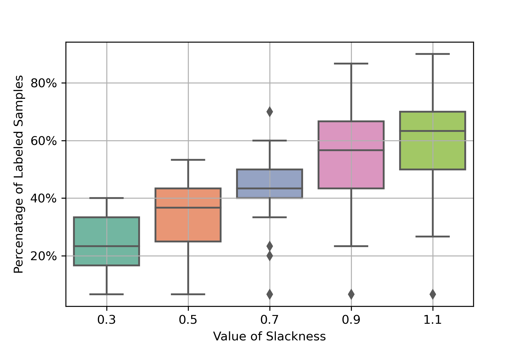
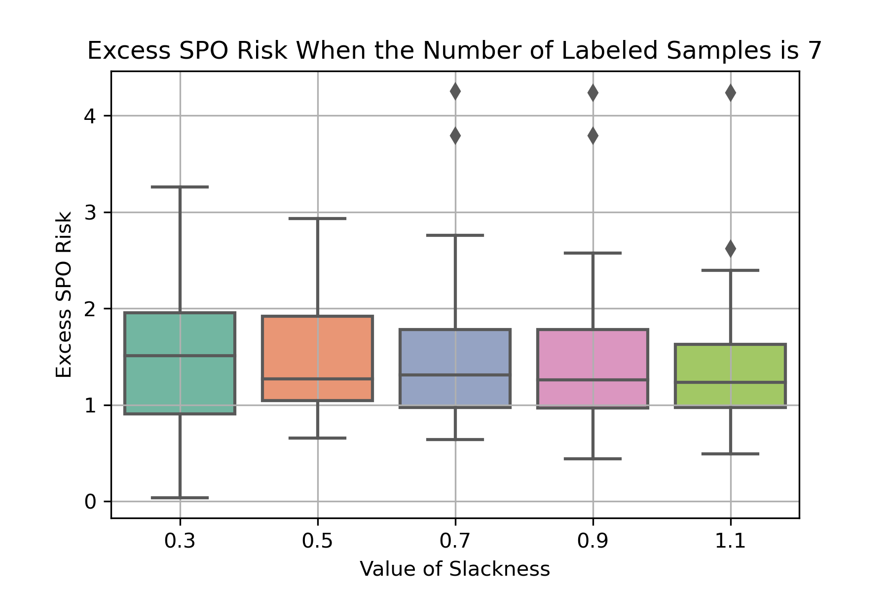
Figure 5: Performance under different settings of slackness in MBAL-SPO

In practice, to find the set the scale for $b_{t}$ and $r_{t}$, we can refer to the rules discussed at the end of Section 4.4, where we set a “burn in” period of $\tilde{T}$ iterations that acquires all labels during the first $\tilde{T}$ iterations. Then, we can use the distribution of values $\{\nu_{S}(h_{T}(x_{t}))\}_{t=1}^{\tilde{T}}$ to inform the value of $b_{T}$. For example, if we want to reduce the number of labels by $50\%$, compared to supervised learning, we can set the scale of $b_{T}$ as the median of $\{\nu_{S}(h_{T}(x_{t}))\}_{t=1}^{\tilde{T}}$.

We also change the value of the minimum label probability $\tilde{p}$ in the soft rejection to see its impact on the performance. Figure 6 shows the percentage of labeled samples in the first 30 samples, and the excess SPO risk when the number of labeled samples is 10.

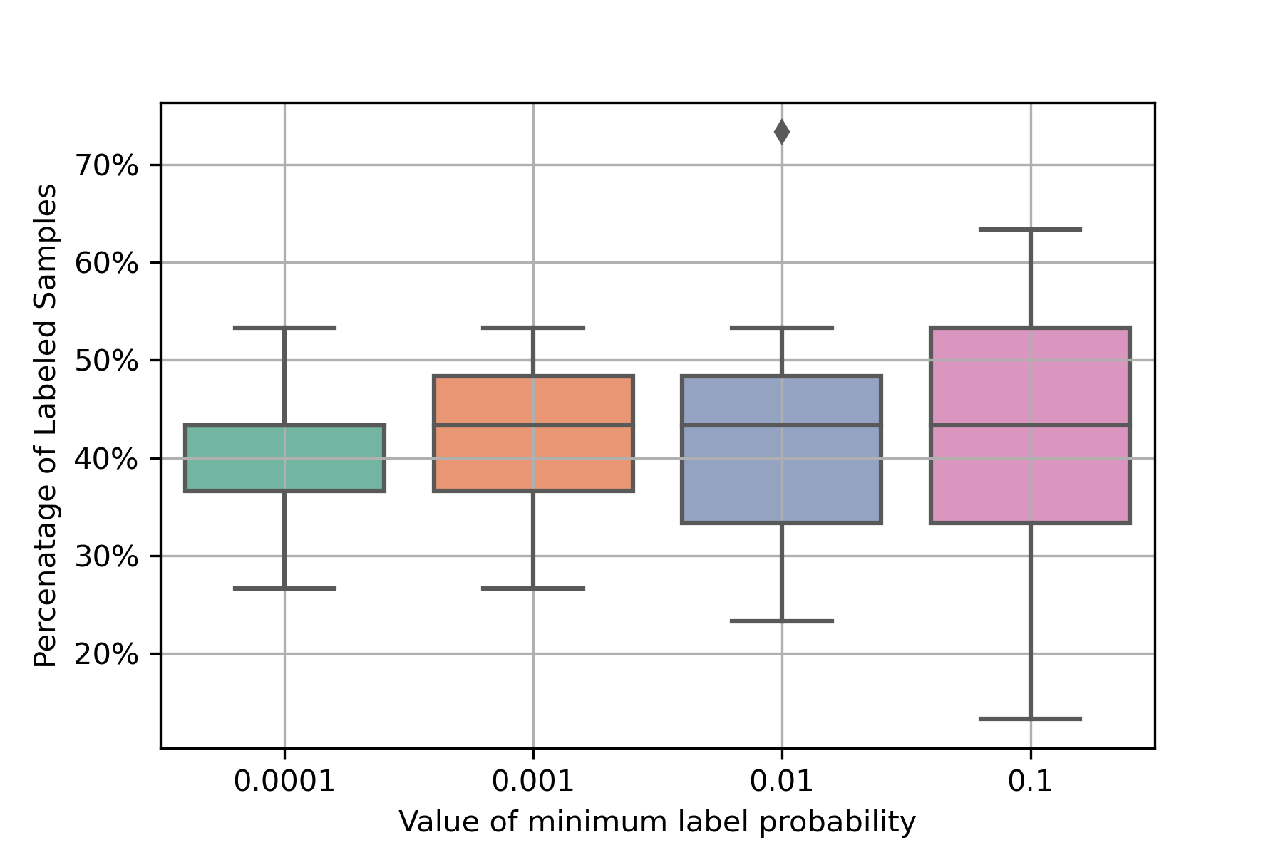
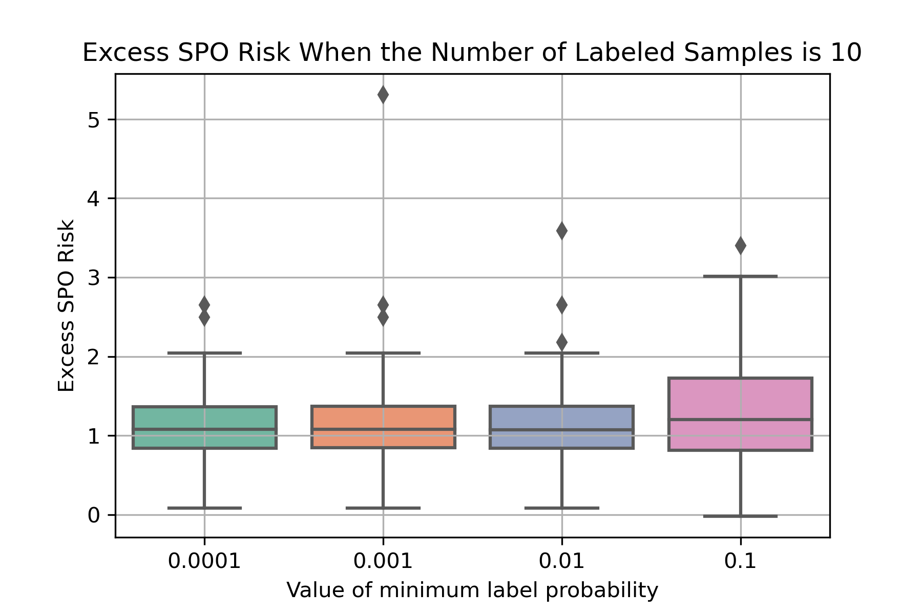
Figure 6: Performance under different settings of $\tilde{p}$

Figure 6 shows that the minimum label probability $\tilde{p}$ has no significant impact on the excess SPO risk. Intuitively, when $\tilde{p}$ is larger, the percentage of labeled samples is larger. In practice, we can set $\tilde{p}$ as a very small positive number that is close to zero.

10.2 Additional Results of Numerical Experiments.

To assess the performance of our active learning algorithm under different noise levels, we change the variance of features and the noise level of labels when generating the data and demonstrate the results in Figures 7 and 8.

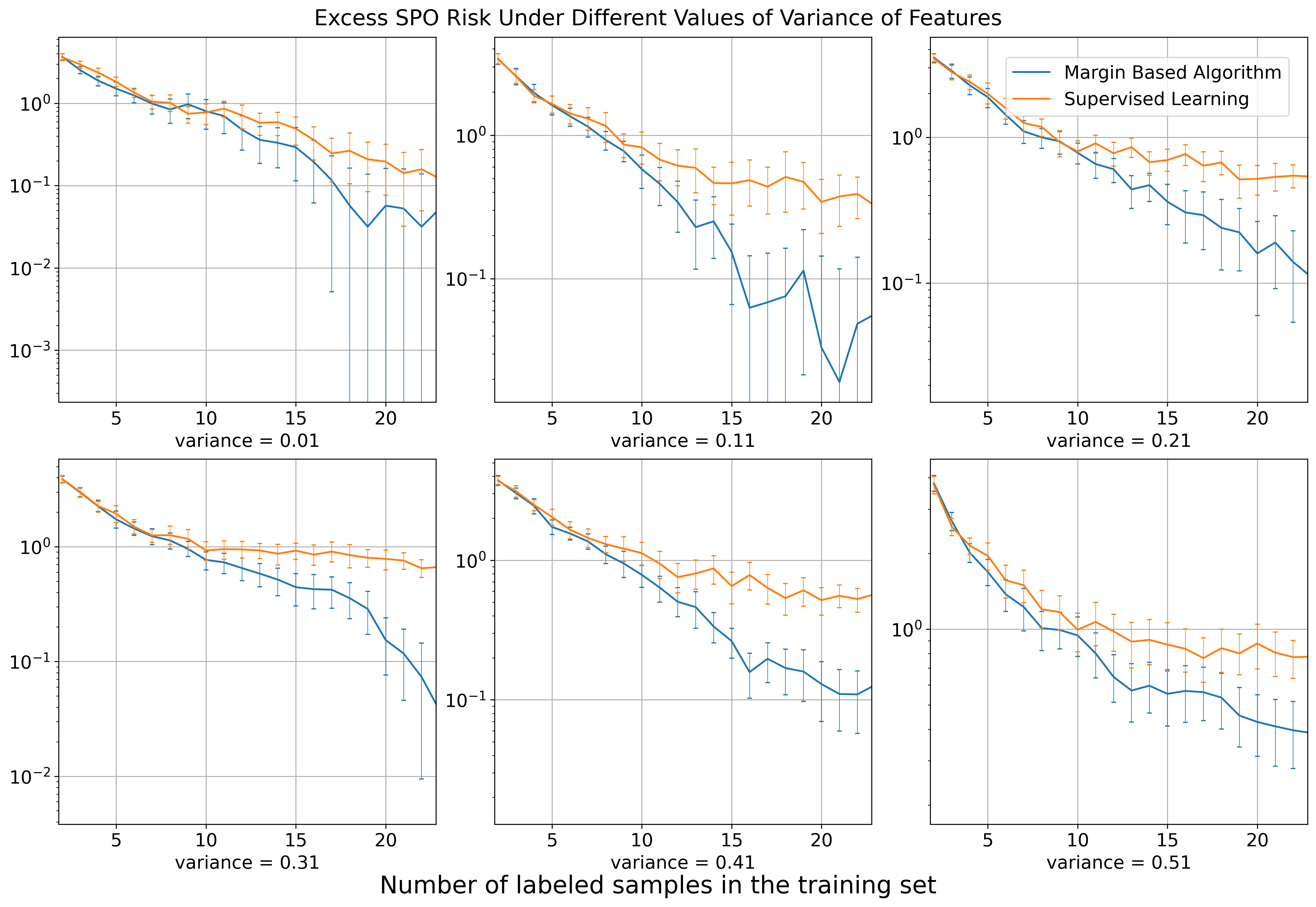
Figure 7: Excess SPO risk during the training process under different variance of features.

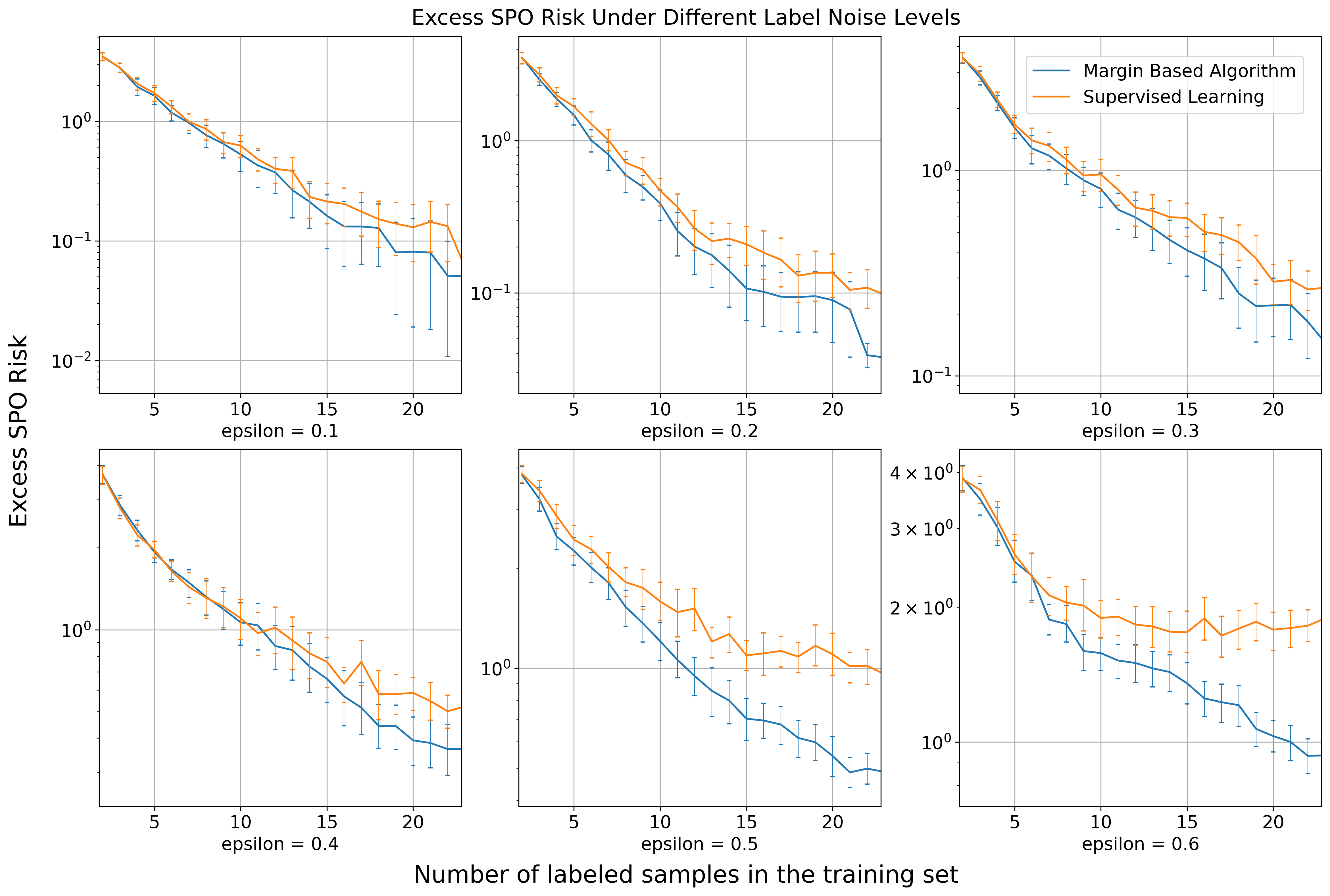
Figure 8: Excess SPO risk during the training process under different noise levels.

Figures 7 and 8 show that when the variance of the features and the noise level of the labels are small, both active learning and supervised learning have close performance. When the variance of features or the noise level of labels is large, our proposed active learning methods perform better than supervised learning.

Recall that the cost vector is gerenated according to $c_{j}=\left[1+(1+b_{j}^{T}x_{i}/\sqrt{p})^{\mathrm{deg}}\right]\epsilon_{j}$. Next, we further show the result when changing the degree of the model. When the degree is not one, the true model is not contained in our hypothesis class. The results in Figure 9 show that when the model has a higher degree, the training process has a higher excess SPO risk at the beginning of the process.

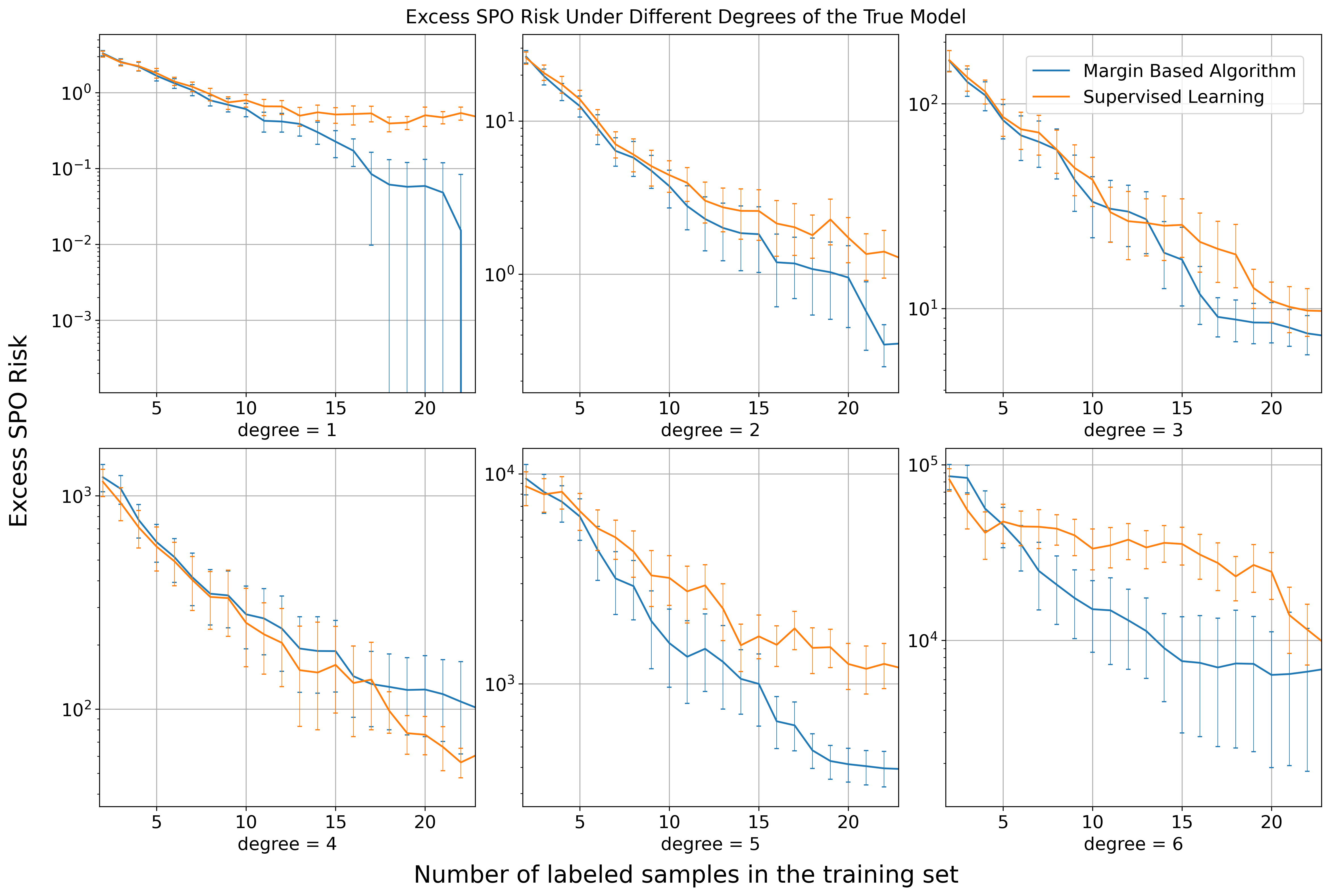
Figure 9: Excess SPO risk during the training process under different noise levels.

10.3 Data Generation for Personalized Pricing

In this section, we provide the parameter values for generating synthetic data in the personalized pricing experiment. Given a coefficient vector $B_{j}\in\mathbb{R}^{5}$ and $A_{j}\in\mathbb{R}^{5}$, the demand function for item $j$ is generated as $d_{j}(p_{i})=\epsilon e^{B_{j}^{T}X+A_{j}^{T}Xp_{i}}$. Here, $\epsilon$ is a noise term drawn from a uniform distribution on $[1-\bar{\epsilon},1+\bar{\epsilon}]$. We set $\bar{\epsilon}=0.1$. $A_{j}^{T}X$ can be viewed as the price elasticity. The customer feature vector is drawn from a mixed Gaussian distribution with seven different centers $\mu_{k}$. The value of these centers $\mu_{k}$, $k=1,2,...,7$ and the value of $A_{j}$ and $B_{j}$, $j=1,2,3$ are carefully chosen so that $h^{*}(X)$ is not a degenerate cost vector for any $\mu_{k}$, $k=1,2,...,7$. Please find the value of these parameters at the end of this appendix. The variance of the feature for each Gaussian distribution is set as $0.01^{2}$, which is on the same scale as the features.

We further have the following monotone constraints for the prices of these three items. Let the decision variable $w_{i,j}$ indicate whether price $i$ is selected for item $j$. Then, the constraints are as follows.

(LABEL:cons:n1) requires each item can only select one price point. (LABEL:cons:n2) and (LABEL:cons:n3) require that the price of item 2 be no less than the price of item 1. (LABEL:cons:n4) and (LABEL:cons:n5) require that the price of item 3 be no less than the price of item 2.

Since the purchase probability is $d_{j}(p_{i})=\epsilon\exp(B_{j}^{T}X+A_{j}^{T}Xp_{i})$, we need to specify the following parameters for generating the purchase probability given the feature $X$: $A_{j}$ and $B_{j}$, $j=1,2,3$. The feature vector is from a mixed Gaussian distribution with seven centers. The optimal prices of three items for these seven centers are $(\$60,\$60,\$60)$, $(\$60,\$80,\$90)$, $(\$90,\$90,\$90)$, $(\$80,\$80,\$80)$, $(\$60,\$60,\$80)$, $(\$80,\$90,\$90)$, and $(\$60,\$60,\$90)$ respectively. To generate such centers, we consider the following values for $X$, $A_{j}$ and $B_{j}$. Define $a_{1}=-0.0202733,b_{1}=-1.19155$, $a_{2}=-0.0133531,b_{2}=-1.45748$, $a_{3}=-0.00540672,b_{3}=-1.22819$. Then, we set

$$A_{1}=\begin{bmatrix}0\\ 0\\ 0\\ 1\\ 0\\ 0\end{bmatrix},A_{2}=\begin{bmatrix}0\\ 0\\ 0\\ 0\\ 1\\ 0\end{bmatrix},A_{3}=\begin{bmatrix}0\\ 0\\ 0\\ 0\\ 0\\ 1\end{bmatrix},B_{1}=\begin{bmatrix}1\\ 0\\ 0\\ 0\\ 0\\ 0\end{bmatrix},B_{2}=\begin{bmatrix}0\\ 1\\ 0\\ 0\\ 0\\ 0\end{bmatrix},B_{3}=\begin{bmatrix}0\\ 0\\ 1\\ 0\\ 0\\ 0\end{bmatrix}.$$

We set the centers of Gaussian distribution for the feature vectors as

$$\mu_{1}=\begin{bmatrix}b_{1}\\ b_{1}\\ b_{1}\\ a_{1}\\ a_{1}\\ a_{1}\end{bmatrix},\mu_{2}=\begin{bmatrix}b_{1}\\ b_{2}\\ b_{3}\\ a_{1}\\ a_{2}\\ a_{3}\end{bmatrix},\mu_{3}=\begin{bmatrix}b_{3}\\ b_{3}\\ b_{3}\\ a_{3}\\ a_{3}\\ a_{3}\end{bmatrix},\mu_{4}=\begin{bmatrix}b_{2}\\ b_{2}\\ b_{2}\\ a_{2}\\ a_{2}\\ a_{2}\end{bmatrix},\mu_{5}=\begin{bmatrix}b_{1}\\ b_{1}\\ b_{2}\\ a_{1}\\ a_{1}\\ a_{2}\end{bmatrix},\mu_{6}=\begin{bmatrix}b_{2}\\ b_{3}\\ b_{3}\\ a_{2}\\ a_{3}\\ a_{3}\end{bmatrix},\mu_{7}=\begin{bmatrix}b_{1}\\ b_{1}\\ b_{3}\\ a_{1}\\ a_{1}\\ a_{3}\end{bmatrix}.$$

References

- Amos and Kolter (2017) Amos B, Kolter JZ (2017) Optnet: Differentiable optimization as a layer in neural networks. International Conference on Machine Learning, 136–145 (PMLR).
- Balcan et al. (2009) Balcan MF, Beygelzimer A, Langford J (2009) Agnostic active learning. Journal of Computer and System Sciences 75(1):78–89.
- Balcan et al. (2007) Balcan MF, Broder A, Zhang T (2007) Margin based active learning. International Conference on Computational Learning Theory, 35–50 (Springer).
- Berthet et al. (2020) Berthet Q, Blondel M, Teboul O, Cuturi M, Vert JP, Bach F (2020) Learning with differentiable pertubed optimizers. Advances in neural information processing systems 33:9508–9519.
- Bertsimas and Kallus (2020) Bertsimas D, Kallus N (2020) From predictive to prescriptive analytics. Management Science 66(3):1025–1044.
- Beygelzimer et al. (2009) Beygelzimer A, Dasgupta S, Langford J (2009) Importance weighted active learning. Proceedings of the 26th annual international conference on machine learning, 49–56.
- Cai et al. (2016) Cai W, Zhang M, Zhang Y (2016) Batch mode active learning for regression with expected model change. IEEE transactions on neural networks and learning systems 28(7):1668–1681.
- Castro et al. (2005) Castro R, Willett R, Nowak R (2005) Faster rates in regression via active learning. NIPS, volume 18, 179–186.
- Chung et al. (2022) Chung TH, Rostami V, Bastani H, Bastani O (2022) Decision-aware learning for optimizing health supply chains. arXiv preprint arXiv:2211.08507 .
- Cohn et al. (1994) Cohn D, Atlas L, Ladner R (1994) Improving generalization with active learning. Machine learning 15(2):201–221.
- Dasgupta et al. (2007) Dasgupta S, Hsu DJ, Monteleoni C (2007) A general agnostic active learning algorithm (Citeseer).
- Demirović et al. (2019) Demirović E, J Stuckey P, Bailey J, Chan J, Leckie C, Ramamohanarao K, Guns T (2019) Predict+ optimise with ranking objectives: Exhaustively learning linear functions. Proceedings of the Twenty-Eighth International Joint Conference on Artificial Intelligence, IJCAI 2019, Macao, China, August 10-16, 2019, 1078–1085 (International Joint Conferences on Artificial Intelligence).
- Demirovic et al. (2020) Demirovic E, J Stuckey P, Guns T, Bailey J, Leckie C, Ramamohanarao K, Chan J (2020) Dynamic programming for predict+ optimise. The Thirty-Fourth AAAI Conference on Artificial Intelligence, AAAI 2020, The Thirty-Second Innovative Applications of Artificial Intelligence Conference, IAAI 2020, The Tenth AAAI Symposium on Educational Advances in Artificial Intelligence, EAAI 2020, New York, NY, USA, February 7-12, 2020, 1444–1451 (AAAI Press).
- Donti et al. (2017) Donti P, Amos B, Kolter JZ (2017) Task-based end-to-end model learning in stochastic optimization. Advances in neural information processing systems 30.
- El Balghiti et al. (2022) El Balghiti O, Elmachtoub AN, Grigas P, Tewari A (2022) Generalization bounds in the predict-then-optimize framework. Mathematics of Operations Research .
- Elmachtoub and Grigas (2022) Elmachtoub AN, Grigas P (2022) Smart “predict, then optimize”. Management Science 68(1):9–26.
- Elmachtoub et al. (2023) Elmachtoub AN, Lam H, Zhang H, Zhao Y (2023) Estimate-then-optimize versus integrated-estimation-optimization: A stochastic dominance perspective. arXiv preprint arXiv:2304.06833 .
- Elmachtoub et al. (2020) Elmachtoub AN, Liang JCN, McNellis R (2020) Decision trees for decision-making under the predict-then-optimize framework. International Conference on Machine Learning, 2858–2867 (PMLR).
- Gao (2022) Gao R (2022) Finite-sample guarantees for wasserstein distributionally robust optimization: Breaking the curse of dimensionality. Operations Research .
- Gao and Saar-Tsechansky (2020) Gao R, Saar-Tsechansky M (2020) Cost-accuracy aware adaptive labeling for active learning. Proceedings of the AAAI Conference on Artificial Intelligence, volume 34, 2569–2576.
- Grigas et al. (2021) Grigas P, Qi M, et al. (2021) Integrated conditional estimation-optimization. arXiv preprint arXiv:2110.12351 .
- Hanneke (2007) Hanneke S (2007) A bound on the label complexity of agnostic active learning. Proceedings of the 24th international conference on Machine learning, 353–360.
- Hanneke (2011) Hanneke S (2011) Rates of convergence in active learning. The Annals of Statistics 333–361.
- Ho and Hanasusanto (2019) Ho CP, Hanasusanto GA (2019) On data-driven prescriptive analytics with side information: A regularized nadaraya-watson approach. URL: http://www. optimization-online. org/DB FILE/2019/01/7043. pdf .
- Ho-Nguyen and Kılınç-Karzan (2022) Ho-Nguyen N, Kılınç-Karzan F (2022) Risk guarantees for end-to-end prediction and optimization processes. Management Science .
- Hu et al. (2022) Hu Y, Kallus N, Mao X (2022) Fast rates for contextual linear optimization. Management Science .
- Kääriäinen (2006) Kääriäinen M (2006) Active learning in the non-realizable case. International Conference on Algorithmic Learning Theory, 63–77 (Springer).
- Kallus and Mao (2023) Kallus N, Mao X (2023) Stochastic optimization forests. Management Science 69(4):1975–1994.
- Kao et al. (2009) Kao Yh, Roy B, Yan X (2009) Directed regression. Advances in Neural Information Processing Systems 22.
- Kotary et al. (2021) Kotary J, Fioretto F, Van Hentenryck P, Wilder B (2021) End-to-end constrained optimization learning: A survey. arXiv preprint arXiv:2103.16378 .
- Krishnamurthy et al. (2017) Krishnamurthy A, Agarwal A, Huang TK, Daumé III H, Langford J (2017) Active learning for cost-sensitive classification. International Conference on Machine Learning, 1915–1924 (PMLR).
- Kuznetsov and Mohri (2015) Kuznetsov V, Mohri M (2015) Learning theory and algorithms for forecasting non-stationary time series. Advances in neural information processing systems 28.
- Liu and Grigas (2021) Liu H, Grigas P (2021) Risk bounds and calibration for a smart predict-then-optimize method. Advances in Neural Information Processing Systems 34.
- Loke et al. (2022) Loke GG, Tang Q, Xiao Y (2022) Decision-driven regularization: A blended model for predict-then-optimize. Available at SSRN 3623006 .
- Mandi and Guns (2020) Mandi J, Guns T (2020) Interior point solving for lp-based prediction+ optimisation. Advances in Neural Information Processing Systems 33:7272–7282.
- Mandi et al. (2020) Mandi J, Stuckey PJ, Guns T, et al. (2020) Smart predict-and-optimize for hard combinatorial optimization problems. Proceedings of the AAAI Conference on Artificial Intelligence, volume 34, 1603–1610.
- Rakhlin et al. (2015a) Rakhlin A, Sridharan K, Tewari A (2015a) Online learning via sequential complexities. J. Mach. Learn. Res. 16(1):155–186.
- Rakhlin et al. (2015b) Rakhlin A, Sridharan K, Tewari A (2015b) Sequential complexities and uniform martingale laws of large numbers. Probability theory and related fields 161:111–153.
- Settles (2009) Settles B (2009) Active learning literature survey (University of Wisconsin-Madison Department of Computer Sciences).
- Sugiyama and Nakajima (2009) Sugiyama M, Nakajima S (2009) Pool-based active learning in approximate linear regression. Machine Learning 75(3):249–274.
- Tang and Khalil (2022) Tang B, Khalil EB (2022) Pyepo: A pytorch-based end-to-end predict-then-optimize library for linear and integer programming. arXiv preprint arXiv:2206.14234 .
- Wainwright (2019) Wainwright MJ (2019) High-dimensional statistics: A non-asymptotic viewpoint, volume 48 (Cambridge University Press).
- Wellner et al. (2013) Wellner J, et al. (2013) Weak convergence and empirical processes: with applications to statistics (Springer Science & Business Media).
- Wilder et al. (2019) Wilder B, Dilkina B, Tambe M (2019) Melding the data-decisions pipeline: Decision-focused learning for combinatorial optimization. Proceedings of the AAAI Conference on Artificial Intelligence, volume 33, 1658–1665.
- Yurtsever and Sra (2022) Yurtsever A, Sra S (2022) CCCP is frank-wolfe in disguise. Oh AH, Agarwal A, Belgrave D, Cho K, eds., Advances in Neural Information Processing Systems, URL https://openreview.net/forum?id=OGGQs4xFHrr.
- Zhu et al. (2022) Zhu T, Xie J, Sim M (2022) Joint estimation and robustness optimization. Management Science 68(3):1659–1677.