Exploiting Fine-Grained DCT Representations for Hiding Image-Level Messages within JPEG Images

Abstract.

Unlike hiding bit-level messages, hiding image-level messages is more challenging, which requires large capacity, high imperceptibility, and high security. Although recent advances in hiding image-level messages have been remarkable, existing schemes are limited to lossless spatial images as covers and cannot be directly applied to JPEG images, the ubiquitous lossy format images in daily life. The difficulties of migration are caused by the lack of targeted design and the loss of details due to lossy decompression and re-compression. Considering that taking DCT densely on $8\times 8$ image patches is the core of the JPEG compression standard, we design a novel model called EFDR, which can comprehensively Exploit Fine-grained DCT Representations and embed the secret image into quantized DCT coefficients to avoid the lossy process. Specifically, we transform the JPEG cover image and hidden secret image into fine-grained DCT representations that compact the frequency and are associated with the inter-block and intra-block correlations. Subsequently, the fine-grained DCT representations are further enhanced by a sub-band features enhancement module. Afterward, a transformer-based invertibility module is designed to fuse enhanced sub-band features. Such a design enables a fine-grained self-attention on each sub-band and captures long-range dependencies while maintaining excellent reversibility for hiding and recovery. To our best knowledge, this is the first attempt to embed a color image of equal size in a color JPEG image. Extensive experiments demonstrate the effectiveness of our EFDR with superior performance.

1. Introduction

Steganography is the science and art of covert communication by sheltering confidential information within publicly available objects without arousing suspicion (Provos and Honeyman, 2003). This technique can date back to the 15-th century when the hidden secret information and the objects used as carriers were both physical levels. With the development of technology, modern steganography is concerned with the digital level. Many kinds of digital media such as images, videos, and audios can be used as steganographic covers, to secretly transmit digital information, among which the research on image steganography using images as carriers receives the most attention (Fridrich, 2009). The task of image steganography is to conceal the secret messages in the cover image to generate the stego one. A well-designed steganographic scheme usually needs to satisfy three basic requirements (Pevný and Fridrich, 2008): the capacity refers to the embedded payload, the imperceptibility regarding the cover and stego being indistinguishable by the naked eyes, and the security against the countermeasure, passive steganalysis.

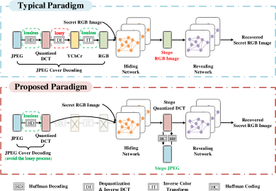
Figure 1. The illustration of the difference between our image-level hiding method and typical image-level hiding methods when the cover is a JPEG image. Unlike typical methods (the top pipeline), we directly hide and recover secret images in the quantized DCT coefficients of the JPEG cover image and the JPEG stego image, respectively, avoiding the process that would cause information loss, and the image type of the stego obtained is also consistent with the original cover type (the bottom pipeline).

On the basis of meeting these basic needs, varieties of steganographic methods (Setiadi et al., 2023) have been designed to pursue superior performance. Traditional content-adaptive steganographic approaches (Holub and Fridrich, 2012; Li et al., 2015) heuristically design the distortion function considering the characteristics of the image itself, and then utilize some coding techniques, e.g., syndrome-trellis codes (STCs) (Filler et al., 2011), to achieve near the minimal distortion embedding under a given payload. However, such methods typically maintain a small embedded payload, at most 1 bit per pixel (Lu et al., 2021). Although several recent deep learning-based methods like SteganoGAN (Zhang et al., 2019) and CHAT-GAN (Tan et al., 2022) have shown significant improvements in hiding capacity, the magnitude of the payload is still on the bit-level, which does not comprehensively exploit the potential of deep hiding. In a seminal work (Baluja, 2017), Baluja successfully hides a color spatial RGB image into another one of the same size, utilizing the structure of pre-processing network - hiding network - revealing network. In comparison to hiding bit-level messages, hiding image-level messages has the following natural advantages. 1) The hidden secret image does not need to be encoded perfectly due to the intrinsic relevance of the image content, which can reduce the difficulty of network learning. 2) It is also acceptable even if there are localized errors in the recovered secret image that do not significantly affect the overall appearance. 3) The amount of payload can reach up to 24 bits per pixel, as the ratio of the hidden secret image and cover image is 1:1.

The success of the pioneering work and the natural advantages of hiding image-level messages make it attract a great deal of attention. Numerous scholars are devoted to researching this field, aiming at improving hiding and revealing performance. Although existing image-level hiding works (Baluja, 2017, 2020; Zhang et al., 2020; Lu et al., 2021; Jing et al., 2021) have achieved remarkable advancement, the cover type targeted by these works is only the lossless spatial RGB image. Practically, JPEG format is the most widely used and spread image format in daily life. It is a lossy format that reduces the size of the image file by compressing visually insensitive information for better storage and transmission (Wallace, 1992), in which the information loss mainly occurs in the quantization and dequantization stages of JPEG image encoding and decoding. Even if the training and testing datasets consist of color JPEG images, typical image-level hiding methods will undergo decompression into the spatial domain before being fed into the network for learning. The obtained stego images are also in a lossless image format, ignoring the problem that the image type of the cover and stego is inconsistent. And the hidden secret image is recovered from the lossless spatial stego with the help of the revealing network (as shown in the typical paradigm of Fig. 1). Additionally, these methods lack JPEG domain knowledge in the model design, which hinders the effective extraction of relevant features. Therefore, their models may treat invisible compression artifacts as common textures, causing image quality degradation.

Concerning these aspects, we propose that the color secret image is directly embedded into the quantized DCT coefficients of the color JPEG image and recovered from the quantized DCT coefficients of the corresponding JPEG stego image, as shown in the proposed paradigm of Fig. 1. Instead of hiding the secret image within the decompressed cover and revealing it from the re-compressed stego, our process can mitigate the information loss problem. To explore the possibility of embedding image-level information in JPEG cover images, we design a novel model called EFDR that aims to fully mine the fine-grained DCT representations being beneficial for hiding and recovery. It comprises three distinct designs: a fine-grained DCT representations module, a sub-band features enhancement module, and a transformer-based invertibility module. Specifically, the first is responsible for transforming the spatial secret image and quantized DCT coefficients of the JPEG cover image into frequency maps, in which each channel represents a frequency sub-band associated with inter-block correlations. And different from conventional frequency components, fine-grained frequency components can be utilized to discover more beneficial representations. The second learns the enhanced sub-band representations adaptively. Besides, to thoroughly integrate the enhanced sub-band representations of cover and secret, the third module adopts a highly reversible structure that can capture long-term dependencies, resulting in appealing outcomes. We evaluate the efficacy of the proposed model through comprehensive experiments and demonstrate its superior performance quantitatively and qualitatively over state-of-the-art (SOTA) methods while also showing its admirable generalization across different datasets.

The main contributions are summarized as follows:

• To our best knowledge, we are the first to propose hiding image-level messages of equal size within a color JPEG image, the ubiquitous lossy format image in daily applications, whereas existing schemes are limited to lossless spatial images as covers. Research on hiding an image within a color JPEG image is of both academic and practical value.

• Unlike learning from image information that has been decompressed (for the hiding network) and then re-compressed (for the revealing network), we propose to hide and reveal the secret image in the quantized DCT coefficients of cover and stego, respectively, vastly mitigating the information loss problem.

• We present a powerful model for the task of hiding image-level messages into a color JPEG image with enhanced fine-grained DCT representations. And we design a sub-band features enhancement module in association with a specific DCT sub-band, and a transformer-based invertibility module combining advantages of long-range dependencies modeling of transformer and reversibility of invertible neural networks.

• Comprehensive experiments on three widely-used datasets show that the proposed method outperforms other SOTA methods by a large margin.

2. Related Work

Recently, researchers have devoted themselves to exploring the possibilities of combining deep learning with image steganography, and have made many impressive achievements. These approaches employ neural networks as either a component in the traditional algorithm (e.g., using deep learning to generate cover images more suitable for steganography (Denis et al., 2020; Shi et al., 2018; Zhou et al., 2020) and design distortion cost to measure whether the pixel is suitable for embedding (Tang et al., 2019; Yang et al., 2020; Tang et al., 2021)), or as an end-to-end solution through which secret messages can be hidden and extracted directly (Hayes and Danezis, 2017; Zhang et al., 2019; Wang et al., 2019; Tan et al., 2022; Baluja, 2017, 2020; Zhang et al., 2020; Lu et al., 2021; Jing et al., 2021). Our work focuses on end-to-end image steganography and we summarize its recent advancement in this section. In terms of the payload magnitude, the related works are classified into embedding information at the bit-level and the image-level.

2.1. Hiding Bit-level Messages

Hayes et al. (Hayes and Danezis, 2017) first proposed an end-to-end model to hide secret information, which defines a three-way game of hiding network, revealing network, and steganalysis network. Nonetheless, the embedding capacity of this approach is only comparable to that of traditional techniques. In addition, there are visual artifacts visible to the naked eyes. To enhance the hiding capacity, imperceptibility, and security, subsequent algorithms designed more elaborate ways to handle confidential information and introduced more advanced modules. Zhang et al. (Zhang et al., 2019) organized binary information into a 3-D tensor concatenated with the image tensor, which can achieve a payload of 4.4 bits per pixel, a 10-fold improvement over the previous approaches. Wang et al. (Wang et al., 2019) and Tan et al. (Tan et al., 2022) followed the information processing way and further improved security and extraction accuracy by incorporating the advanced Inception-ResNet module and channel attention mechanism, respectively. However, the embedding capacity of the aforementioned algorithms remains at the bit-level.

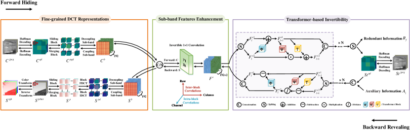
Figure 2. Overall model architecture. In the forward hiding process, a spatial RGB secret image $S^{rgb}$ is hidden in a JPEG cover image $C^{jpeg}$ through a fine-grained DCT representations module, a sub-band features enhancement module, and a transformer-based invertibility module to generate a JPEG stego image $St^{jpeg}$, together with the redundant information $R_{f}$. In the backward revealing process, the JPEG stego image $St^{jpeg}$ and auxiliary information $A^{z}$ are fed to recover the secret image. Here, $A^{z}$ is set as an all-zero tensor. Therefore, only the stego image is actually required to extract the secret image $S^{rgb}$, ensuring blind extraction.

2.2. Hiding Image-level Messages

Baluja (Baluja, 2017) first attempted to hide a color image within another one using deep learning. To achieve this goal, a model consisting of three modules is designed, in which the preparation network extracts fundamental features of the secret image, the hiding network fuses the extracted features into a cover image to obtain a stego image, and the revealing network restores the secret image from the stego image. Because the amount of information needed to hide is large, the risk of secret images being disclosed is correspondingly higher. The extension work (Baluja, 2020) further explored the problem that the secret image may be exposed through residuals between cover and stego. Inspired by the universal adversarial perturbations in the field of adversarial example, Zhang et al. (Zhang et al., 2020) designed a cover-agnostic manner to hide an image, which mitigates the risk of exposure by encoding the secret image into a universal latent representations. Lu et al. (Lu et al., 2021) regarded the task of hiding an image as an invertible problem in image domain transformation. They introduced the invertible network to perform embedding and extraction through its forward and backward processes, resulting in significant improvements in both visual quality and security. Jing et al. (Jing et al., 2021) also utilized the invertible network and implemented it in the wavelet domain. A low-frequency wavelet loss was also designed to control the embedding distribution of secret information in different frequency bands, which further promoted security. Despite that, the cover type adopted by these schemes is all the lossless spatial RGB image, without taking into account the more widely used JPEG images. Moreover, these methods lack specific design and are unsuitable when the cover is a JPEG image.

3. Method

In this section, we propose a novel model called EFDR that aims to hide image-level messages into a color JPEG image with high imperceptibility and high security. For the sake of convenience, we summarize the symbols used in this paper in Table 1.

Table 1. The summary of symbols used in this paper.

Symbols	Descriptions
$C^{jpeg}$	JPEG cover image: the image to hide secret information
$C^{qd}$	quantized DCT coefficients of JPEG cover
$C^{pqd}$	a set of $8\times 8$ quantized DCT coefficients patches of JPEG cover
$C^{b}$	decoupling frequency maps of JPEG cover
$S^{rgb}$	spatial RGB secret image: the image to be hidden
$S^{ycbcr}$	the YCbCr transformation of secret
$S^{p}$	a set of $8\times 8$ YCbCr transformation patches of secret
$S^{pd}$	a set of $8\times 8$ DCT coefficients patches of secret
$S^{b}$	decoupling frequency maps of secret
$St^{jpeg}$	JPEG stego image: the image containing secret information
$St^{qd}$	quantized DCT coefficients of JPEG stego
$F^{e}$	the enhanced sub-band feature maps
$R_{f}$	redundant information: the lost information in hiding process
$A^{z}$	auxiliary information: the information to help reveal secret

3.1. Overview

Fig. 2 shows the framework of the proposed EFDR, containing three key components: a fine-grained DCT representations module, a sub-band features enhancement module, and a transformer-based invertibility module. In the forward hiding process, a pair of JPEG cover image $C^{jpeg}$ and spatial RGB secret image $S^{rgb}$ are as the input. They are converted into fine-grained frequency maps, in which each channel denotes a frequency sub-band. Then, after sub-band features enhancement and a series of transformer-based invertible sub-modules, the quantized DCT coefficients of JPEG stego $St^{qd}$ can be obtained, together with the lost redundant information $R_{f}$. $St^{qd}$ can be transformed into JPEG image $St^{jpeg}$ by Huffman coding. Conversely, in the backward revealing process, $St^{jpeg}$ and auxiliary information $A^{z}$ go through the inverse process of the above three modules to recover $S^{rgb}$. The hiding and revealing processes can be expressed as

$$(St^{jpeg},R_{f})=\textbf{T}(\textbf{E}(\textbf{F}(C^{jpeg},S^{rgb})))$$

(1) $$(C^{jpeg},S^{rgb})=\textbf{F}^{-1}(\textbf{E}^{-1}(\textbf{T}^{-1}(St^{jpeg},A^{z})))$$

In Eq. (1), $\textbf{F}(\mathchoice{\mathbin{\vbox{\hbox{\scalebox{0.5}{$\displaystyle\bullet$}}}}}{\mathbin{\vbox{\hbox{\scalebox{0.5}{$\textstyle\bullet$}}}}}{\mathbin{\vbox{\hbox{\scalebox{0.5}{$\scriptstyle\bullet$}}}}}{\mathbin{\vbox{\hbox{\scalebox{0.5}{$\scriptscriptstyle\bullet$}}}}})$, $\textbf{E}(\mathchoice{\mathbin{\vbox{\hbox{\scalebox{0.5}{$\displaystyle\bullet$}}}}}{\mathbin{\vbox{\hbox{\scalebox{0.5}{$\textstyle\bullet$}}}}}{\mathbin{\vbox{\hbox{\scalebox{0.5}{$\scriptstyle\bullet$}}}}}{\mathbin{\vbox{\hbox{\scalebox{0.5}{$\scriptscriptstyle\bullet$}}}}})$, $\textbf{T}(\mathchoice{\mathbin{\vbox{\hbox{\scalebox{0.5}{$\displaystyle\bullet$}}}}}{\mathbin{\vbox{\hbox{\scalebox{0.5}{$\textstyle\bullet$}}}}}{\mathbin{\vbox{\hbox{\scalebox{0.5}{$\scriptstyle\bullet$}}}}}{\mathbin{\vbox{\hbox{\scalebox{0.5}{$\scriptscriptstyle\bullet$}}}}})$ and $\textbf{F}^{-1}(\mathchoice{\mathbin{\vbox{\hbox{\scalebox{0.5}{$\displaystyle\bullet$}}}}}{\mathbin{\vbox{\hbox{\scalebox{0.5}{$\textstyle\bullet$}}}}}{\mathbin{\vbox{\hbox{\scalebox{0.5}{$\scriptstyle\bullet$}}}}}{\mathbin{\vbox{\hbox{\scalebox{0.5}{$\scriptscriptstyle\bullet$}}}}})$, $\textbf{E}^{-1}(\mathchoice{\mathbin{\vbox{\hbox{\scalebox{0.5}{$\displaystyle\bullet$}}}}}{\mathbin{\vbox{\hbox{\scalebox{0.5}{$\textstyle\bullet$}}}}}{\mathbin{\vbox{\hbox{\scalebox{0.5}{$\scriptstyle\bullet$}}}}}{\mathbin{\vbox{\hbox{\scalebox{0.5}{$\scriptscriptstyle\bullet$}}}}})$, $\textbf{T}^{-1}(\mathchoice{\mathbin{\vbox{\hbox{\scalebox{0.5}{$\displaystyle\bullet$}}}}}{\mathbin{\vbox{\hbox{\scalebox{0.5}{$\textstyle\bullet$}}}}}{\mathbin{\vbox{\hbox{\scalebox{0.5}{$\scriptstyle\bullet$}}}}}{\mathbin{\vbox{\hbox{\scalebox{0.5}{$\scriptscriptstyle\bullet$}}}}})$ represent the three modules and their inverse processes respectively. The modules details and loss functions will be further provided in the following.

3.2. Fine-grained DCT Representations

As shown in the leftmost of Fig. 2, we convert the JPEG cover image and secret RGB image into fine-grained frequency components that facilitate hiding and revealing. The processing of JPEG cover image $C^{jpeg}\in{\mathbb{R}^{(3,H,W)}}$ and secret RGB image $S^{rgb}\in{\mathbb{R}^{(3,H,W)}}$ is slightly different, where the superscript $(3,H,W)$ denote the shape with $(channel,height,width)$. Concretely, for $C^{jpeg}$, the quantized DCT coefficients $C^{qd}\in{\mathbb{R}^{(3,H,W)}}$ is firstly extracted by Huffman decoding. After that, we can acquire a set of quantized DCT coefficients blocks $C^{pqd}\in{\mathbb{R}^{(3\times{\frac{H}{8}}\times{\frac{W}{8}},8,8)}}$ through a fixed size $8\times 8$ sliding window. Each value in $C^{pqd}$ corresponds to the intensity of 192 frequency bands of 3 color channels. To make the frequency components more compact, we flatten and reshape $C^{pqd}$ to form fully decoupling frequency maps $C^{b}\in{\mathbb{R}^{(192,\frac{H}{8},\frac{W}{8})}}$, where the values in each channel represent the intensity of a frequency sub-band. In this way, the original input is reconstructed to fine-grained frequency-aware information that contains both the intra-block correlations in the channel dimension and the inter-block correlations in the space dimension. For the processing of the $S^{rgb}$, there are two more steps, namely color conversion to YCbCr space to obtain $S^{ycbcr}\in{\mathbb{R}^{(3,H,W)}}$ and dense DCT transform on $8\times 8$ YCbCr transformation patches $S^{p}\in{\mathbb{R}^{(3\times{\frac{H}{8}}\times{\frac{W}{8}},8,8)}}$ to attain DCT coefficients patches, denoted by $S^{pd}\in{\mathbb{R}^{(3\times{\frac{H}{8}}\times{\frac{W}{8}},8,8)}}$. In the backward revealing process, just perform the inverse operations of the previous procedures.

3.3. Sub-band Features Enhancement

The structure of this module is shown in the middle of Fig. 2, we first concatenate the decoupling frequency maps $C^{b}$ and $S^{b}$ in the channel dimension. Subsequently, an invertible $1\times 1$ convolution layer (Kingma and Dhariwal, 2018) is applied to their concatenation to adaptively extract the most informative frequency features. The invertible $1\times 1$ convolution is a kind of convolution commonly used for flow-based generative models. It performs a linear transformation on the input feature maps by multiplying them with a random rotation weight matrix with the nonzero determinant. And its inverse operation is to multiply the output feature maps with the inverse of the weight matrix to restore the input feature maps. Here, the number of convolution kernels is set to 384, which is equal to the sum of the DCT frequency modes of the color JPEG image and the secret image. Such a design can make each element in the enhanced feature maps (denoted by $F^{e}\in{\mathbb{R}^{(384,\frac{H}{8},\frac{W}{8})}}$) associated with a specific DCT sub-band.

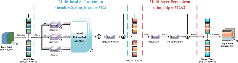
Figure 3. The detailed structure of our $\Phi(\mathchoice{\mathbin{\vbox{\hbox{\scalebox{0.5}{$\displaystyle\bullet$}}}}}{\mathbin{\vbox{\hbox{\scalebox{0.5}{$\textstyle\bullet$}}}}}{\mathbin{\vbox{\hbox{\scalebox{0.5}{$\scriptstyle\bullet$}}}}}{\mathbin{\vbox{\hbox{\scalebox{0.5}{$\scriptscriptstyle\bullet$}}}}})$, $\Psi(\mathchoice{\mathbin{\vbox{\hbox{\scalebox{0.5}{$\displaystyle\bullet$}}}}}{\mathbin{\vbox{\hbox{\scalebox{0.5}{$\textstyle\bullet$}}}}}{\mathbin{\vbox{\hbox{\scalebox{0.5}{$\scriptstyle\bullet$}}}}}{\mathbin{\vbox{\hbox{\scalebox{0.5}{$\scriptscriptstyle\bullet$}}}}})$, and $\Upsilon(\mathchoice{\mathbin{\vbox{\hbox{\scalebox{0.5}{$\displaystyle\bullet$}}}}}{\mathbin{\vbox{\hbox{\scalebox{0.5}{$\textstyle\bullet$}}}}}{\mathbin{\vbox{\hbox{\scalebox{0.5}{$\scriptstyle\bullet$}}}}}{\mathbin{\vbox{\hbox{\scalebox{0.5}{$\scriptscriptstyle\bullet$}}}}})$, i.e., a 1-layer Pre-LN transformer block, which consists of a multi-head self-attention and a multi-layer perceptron. Concretely, the dimension of input and output are the same. We employ $heads=8$ parallel attention layers, as well as the dimension $dim\_heads=512$ of the inner layer. And in the multi-layer perceptron, the dimension $dim\_mlp=512\times 2$ of inner layer.

3.4. Transformer-based Invertibility

Our transformer-based invertibility module, shown in the rightmost of Fig. 2, is derived from invertible neural networks (Dinh et al., 2017; Xiao et al., 2020) and the vision transformer (Dosovitskiy et al., 2021), both of which are good at image-related tasks. Currently, many image-related tasks have employed invertible neural networks, such as image re-scaling (Xiao et al., 2020), image decolorization (Zhao et al., 2021), and image translation (Ouderaa and Worrall, 2019). The vision transformer is also widely applied to image-related fields, including image classification (Liu et al., 2021), semantic segmentation (Zheng et al., 2021), and object detection (Carion et al., 2020). An invertible sub-module adopts the bijective affine coupling layer with shared parameters to perform forward and backward operations so that the details can be preserved as much as possible to achieve the reversibility of input and output. To further enhance representation and global dependency modeling, the transformer is introduced as the backbone. To be more specific, for the $l$-th invertible sub-module, $1\leq{l}\leq{N}$, we adopt an additive transform for branch 1 ($F^{e1}_{l}\in{\mathbb{R}^{(192,\frac{H}{8},\frac{W}{8})}}$) and an enhanced affine transform for branch 2 ($F^{e2}_{l}\in{\mathbb{R}^{(192,\frac{H}{8},\frac{W}{8})}}$). Thus, the forward process of the bijective affine coupling layer can be formulated as

$$F^{e1}_{l+1}=F^{e1}_{l}+\Phi(F^{e2}_{l})$$

(2) $$F^{e2}_{l+1}=F^{e2}_{l}\odot{\textbf{exp}(\Psi(F^{e1}_{l+1}))}+\Upsilon(F^{e1}_{l+1})$$

In Eq. (2), $\Phi(\mathchoice{\mathbin{\vbox{\hbox{\scalebox{0.5}{$\displaystyle\bullet$}}}}}{\mathbin{\vbox{\hbox{\scalebox{0.5}{$\textstyle\bullet$}}}}}{\mathbin{\vbox{\hbox{\scalebox{0.5}{$\scriptstyle\bullet$}}}}}{\mathbin{\vbox{\hbox{\scalebox{0.5}{$\scriptscriptstyle\bullet$}}}}})$, $\Psi(\mathchoice{\mathbin{\vbox{\hbox{\scalebox{0.5}{$\displaystyle\bullet$}}}}}{\mathbin{\vbox{\hbox{\scalebox{0.5}{$\textstyle\bullet$}}}}}{\mathbin{\vbox{\hbox{\scalebox{0.5}{$\scriptstyle\bullet$}}}}}{\mathbin{\vbox{\hbox{\scalebox{0.5}{$\scriptscriptstyle\bullet$}}}}})$, and $\Upsilon(\mathchoice{\mathbin{\vbox{\hbox{\scalebox{0.5}{$\displaystyle\bullet$}}}}}{\mathbin{\vbox{\hbox{\scalebox{0.5}{$\textstyle\bullet$}}}}}{\mathbin{\vbox{\hbox{\scalebox{0.5}{$\scriptstyle\bullet$}}}}}{\mathbin{\vbox{\hbox{\scalebox{0.5}{$\scriptscriptstyle\bullet$}}}}})$ denote the transformer block. Here, we adopt a 1-layer Pre-LN transformer, as shown in Fig. 3. The Pre-LN transformer, which puts the layer normalization before the multi-head self-attention and multi-layer perceptron, compared with the Post-LN transformer, has a more stable gradient distribution, and the gradient norm is almost constant between layers, which is more conducive to optimization by the optimizer (Xiong et al., 2020). $\odot$ and $\textbf{exp}(\mathchoice{\mathbin{\vbox{\hbox{\scalebox{0.5}{$\displaystyle\bullet$}}}}}{\mathbin{\vbox{\hbox{\scalebox{0.5}{$\textstyle\bullet$}}}}}{\mathbin{\vbox{\hbox{\scalebox{0.5}{$\scriptstyle\bullet$}}}}}{\mathbin{\vbox{\hbox{\scalebox{0.5}{$\scriptscriptstyle\bullet$}}}}})$ are the Hadamard product and Exponential function, respectively. Correspondingly, the inverse operation is

$$F^{e2}_{l}=(F^{e2}_{l+1}-\Upsilon(F^{e1}_{l+1}))\odot\textbf{exp}(-\Psi(F^{e1}_{l+1}))$$

(3) $$F^{e1}_{l}=F^{e1}_{l+1}-\Phi(F^{e2}_{l})$$

Note that $\textbf{exp}(\mathchoice{\mathbin{\vbox{\hbox{\scalebox{0.5}{$\displaystyle\bullet$}}}}}{\mathbin{\vbox{\hbox{\scalebox{0.5}{$\textstyle\bullet$}}}}}{\mathbin{\vbox{\hbox{\scalebox{0.5}{$\scriptstyle\bullet$}}}}}{\mathbin{\vbox{\hbox{\scalebox{0.5}{$\scriptscriptstyle\bullet$}}}}})$ is omitted in the figure.

3.5. Loss Functions

The total loss $\mathcal{L}_{total}$ consists of two parts: the hiding loss $\mathcal{L}_{hi}$ to ensure imperceptibility and security, and the revealing loss $\mathcal{L}_{re}$ to ensure the recovery quality. $\mathcal{L}_{total}$ is equal to the sum of the two losses.

Hiding loss. The forward hiding process aims to embed $S^{rgb}$ into $C^{jpeg}$ to generate $St^{jpeg}$. To achieve imperceptibility and security, $St^{jpeg}$ is required to be close to $C^{jpeg}$. Thus, $\mathcal{L}_{hi}$ is defined as follows

(4) $$\mathcal{L}_{hi}=MSE(St^{jpeg},C^{jpeg})$$

Revealing loss. The backward revealing process aims to losslessly extract $S^{rgb}$ from $St^{jpeg}$. Toward this goal, we define the $\mathcal{L}_{re}$ as follows

(5) $$\mathcal{L}_{re}=MSE(S^{rgb}_{ex},S^{rgb})$$

where $S^{rgb}_{ex}$ represents the actual extracted secret image. It should be noted that we do not set any restrictions on the forward redundant information $R_{f}$ and the recovered cover JPEG image, because these two variables are less important in the whole hiding and revealing tasks.

4. Experiments

4.1. Experimental Settings

Datasets. We conduct experiments on three image datasets: COCO (Lin et al., 2014) and ImageNet (Russakovsky et al., 2015), and a standard steganography research dataset BOSSBase (Bas et al., 2011). 10000 and 4000 images are randomly selected from COCO as the training set and test set, respectively. ImageNet and BOSSBase only serve as test sets, and the number of images is also 4000. All images are center-cropped to the size of $128\times{128}$ and re-compressed into JPEG format with two commonly used quality factors (QFs) 75 and 95. Although some images in these datasets may suffer from double/multiple JPEG compression, their use does not jeopardize the feasibility of the proposed scheme (Tang et al., 2019). Double/multiple JPEG compression images are more common in practice.

Benchmarks. To verify the effectiveness of our method, we compare it with SOTA image-level hiding works that hide a color image into another one of equal size, including Baluja (Baluja, 2020), UDH (Zhang et al., 2020), ISN (Lu et al., 2021), and HiNet (Jing et al., 2021). For a fair comparison, we retrain and evaluate the models using the same datasets as ours, with the parameters following the default settings in these references.

Evaluation metrics. Four metrics are adopted to measure the image quality of cover/stego and secret/recovery pairs, such as peak signal-to-noise ratio (PSNR) and structural similarity (SSIM), two commonly used objective evaluation indicators (Wang et al., 2004), average pixel discrepancy (APD) calculated by $L1$ norm, and learned perceptual image patch similarity (LPIPS), which is more consistent with human visual perception (Zhang et al., 2018). PSNR /SSIM with larger values and APD/LPIPS with smaller values indicate higher image quality. In addition, we employ two representative JPEG steganalyzers to evaluate the security performance of our method, including handcrafted features-based DCTR (Holub and Fridrich, 2015) and deep learning-based SRNet (Boroumand et al., 2019).

Implementation details. Our EFDR is implemented with PyTorch, and the NVIDIA GeForce RTX 2080 Ti GPU is used for acceleration. We adopt the Adam optimizer with $betas=(0.5,0.999)$, $eps=1e^{-6}$, and $weight\_decay=5e^{-4}$. The initial learning rate is $5e^{-4}$, which is dynamically adjusted by the ReduceLROnPlateau learning strategy with the factor of 0.5. The mini-batch size is 4, containing two randomly selected cover/secret pairs. And the number of total training epoch is 200. Both $QF=75$ and $QF=95$, our model contains 12 transformer-based invertible sub-modules, and each of them uses three 1-layer Pre-LN transformer blocks.

Table 2. Quantitative quality comparisons on different datasets with QFs of 75 and 95. Value1/value2 represent the assessment value calculated by the cover/stego and secret/recovery image pairs, respectively, under the corresponding metrics. The best and second-best results separately are marked in bold and underline.

QFs

Methods

COCO

ImageNet

BOSSBase

PSNR(dB)$\uparrow$

SSIM$\uparrow$

APD$\downarrow$

LPIPS$\downarrow$

PSNR(dB)$\uparrow$

SSIM$\uparrow$

APD$\downarrow$

LPIPS$\downarrow$

PSNR(dB)$\uparrow$

SSIM$\uparrow$

APD$\downarrow$

LPIPS$\downarrow$

75

Baluja (Baluja, 2020)

24.24/21.55

.847/.754

11.54/18.86

.188/.393

24.68/21.55

.851/.746

11.75/19.30

.182/.389

26.82/23.38

.842/.820

8.82/16.49

.217/.409

UDH (Zhang et al., 2020)

23.94/21.89

.820/.748

8.62/18.26

.173/.301

24.69/21.77

.825/.737

8.48/18.98

.168/.306

24.81/23.54

.791/.805

8.62/16.30

.252/.302

ISN (Lu et al., 2021)

24.43/24.47

.834/.858

8.54/7.51

.180/.169

25.16/24.88

.836/.859

8.63/7.62

.177/.170

26.03/29.30

.821/.909

7.86/5.94

.234/.120

HiNet (Jing et al., 2021)

16.90/20.17

.489/.662

21.50/16.37

.444/.407

17.43/20.42

.504/.659

20.87/16.67

.433/.408

17.26/23.21

.446/.751

21.14/12.55

.561/.389

EFDR

32.16/35.30

.928/.934

4.72/3.70

.024/.017

31.92/35.38

.923/.935

4.94/3.78

.027/.018

35.90/37.17

.944/.950

3.12/2.96

.028/.014

95

Baluja (Baluja, 2020)

24.44/21.58

.859/.754

10.92/18.81

.183/.393

24.88/21.58

.860/.746

11.23/19.23

.178/.389

27.03/23.40

.840/.821

8.12/16.54

.196/.408

UDH (Zhang et al., 2020)

24.25/21.87

.818/.738

7.38/18.30

.159/.307

24.96/21.61

.825/.719

7.24/19.29

.151/.319

25.12/23.18

.797/.764

7.78/16.65

.225/.325

ISN (Lu et al., 2021)

24.42/23.38

.843/.832

7.60/9.01

.178/.201

25.08/23.73

.843/.831

7.77/9.46

.176/.202

25.42/27.43

.812/.879

7.86/7.39

.230/.161

HiNet (Jing et al., 2021)

17.59/20.03

.543/.611

17.85/16.82

.380/.448

18.14/20.27

.556/.608

17.29/17.04

.373/.450

17.99/22.52

.509/.679

17.65/13.52

.473/.424

EFDR

34.25/32.08

.925/.887

3.89/5.17

.013/.048

34.03/32.16

.920/.891

4.08/5.21

.013/.046

35.71/33.66

.909/.906

3.30/4.30

.018/.053

4.2. Comparisons with SOTA Methods

Quantitative quality evaluation. Table 2 reports the numerical comparisons of our EFDR with Baluja (Baluja, 2020), UDH (Zhang et al., 2020), ISN (Lu et al., 2021), and HiNet (Jing et al., 2021) in terms of the four image quality metrics. It can be observed that the proposed EFDR significantly outperforms other approaches in terms of both hiding and revealing performance. For $QF=75$, compared with the second-best results, our EFDR can achieve a PSNR improvement of 7.73/10.83 dB, 6.76/10.50 dB, and 9.08/7.87 dB on COCO, ImageNet, and BOSSBase datasets, respectively. Regarding $QF=95$, we supply 9.81/8.70 dB, 8.95/8.43 dB, and 8.68/6.23 dB PSNR advancement. Similar performance betterment can be seen in SSIM, APD, and LPIPS. It is noteworthy that although our model only uses the COCO dataset for training, it still provides excellent results on the other two datasets, which indicates that our model has a favorable generalization ability.

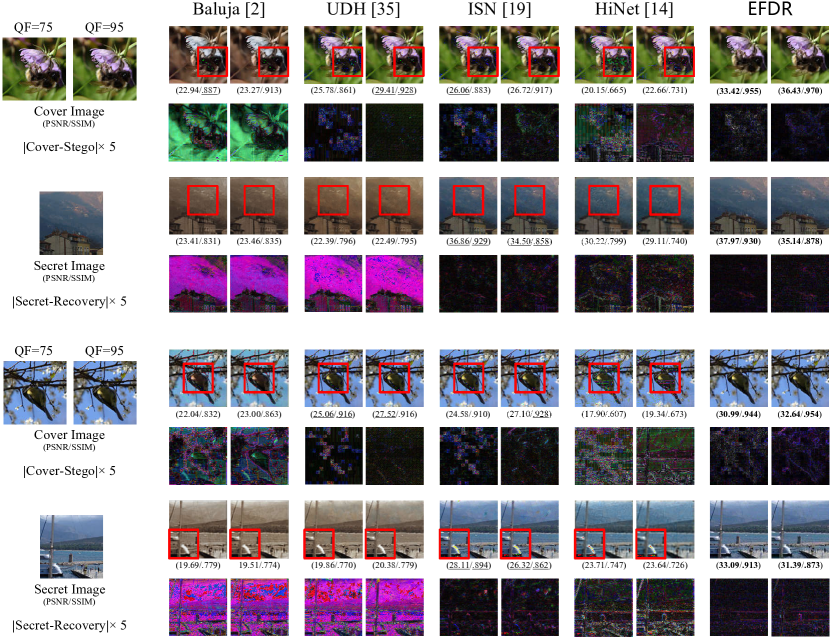
Figure 4. Visualization comparisons of our EFDR with Baluja (Baluja, 2020), UDH (Zhang et al., 2020), ISN (Lu et al., 2021), and HiNet (Jing et al., 2021). To illustrate the differences between the original and generated images, the pixel-wise residuals are magnified by 5 times. The red boxes mark the color distortion, blurring, noise, and other artifacts that are visible to the naked eyes in the stegos and the recovered secret images generated by the comparison methods.

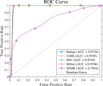
Figure 5. Comparisons of anti-steganalyzer DCTR when QF is 75.

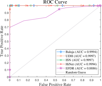
Figure 6. Comparisons of anti-steganalyzer DCTR when QF is 95.

Table 3. Comparisons of anti-steganalyzer SRNet.

Methods	Accuracy(%)$\downarrow$ $\pm$ std
	QF=75	QF=95
Baluja (Baluja, 2020)	90.93 $\pm$ .196	97.80 $\pm$ .105
UDH (Zhang et al., 2020)	98.73 $\pm$ .079	99.93 $\pm$ .019
ISN (Lu et al., 2021)	91.43 $\pm$ .189	97.80 $\pm$ .104
HiNet (Jing et al., 2021)	99.50 $\pm$ .050	99.95 $\pm$ .016
EFDR	80.32 $\pm$ .269	82.05 $\pm$ .255

Table 4. Ablation Study on different numbers of sub-module selection in transformer-based invertibility module.

	Nums.	PSNR(dB)$\uparrow$	SSIM$\uparrow$	APD$\downarrow$	LPIPS$\downarrow$
QF=75	16	9.70/15.83	.261/.497	49.55/21.67	.366/.433
	12	31.92/35.38	.923/.935	4.94/3.78	.027/.018
	8	28.98/31.27	.886/.912	6.06/4.67	.053/.031
	4	27.52/24.26	.772/.643	8.01/12.64	.146/.289
QF=95	16	32.01/27.22	.793/.774	6.98/8.78	.031/.077
	12	34.03/32.16	.920/.891	4.08/5.21	.013/.046
	8	10.49/13.45	.134/.306	68.70/37.19	.625/.504
	4	30.18/29.95	.843/.849	6.37/6.53	.036/.047

Qualitative quality evaluation. Visualization comparisons between our EFDR and the other four methods are shown in Fig. 4. Two examples shown are from ImageNet and BOSSBase datasets. We can observe that both the generated stego image and the recovered secret image are visually pleasing, with smaller visual residuals, which indicates that our model has nice hiding and revealing performance. In contrast, the comparison methods have difficulties in effectively extracting relevant features as they learn from image information that has been decompressed (for the hiding network) and then re-compressed (for the revealing network), and lack the utilization of JPEG image domain knowledge in their model design. Instead, the information differences caused by decompression and re-compression may be amplified, resulting in visible color distortion, blocking, blurring, and banding artifacts in the generated stego and recovered secret image.

JPEG steganalysis. Steganalysis, another essential metric, evaluates the statistical security for hiding methods. It measures the likelihood of distinguishing stego images from cover images by revealing alterations in statistical features caused by embedding. Currently, mainstream steganalysis methods can be divided into two categories: traditional handcrafted features-based methods and deep learning-based methods. In this subsection, we select two representative JPEG image steganalyzers to evaluate the anti-steganalysis ability of our EFDR and the comparison methods, including handcrafted features-based DCTR (Holub and Fridrich, 2015) and deep learning-based SRNet (Boroumand et al., 2019). Specifically, we select 2000 pairs of cover images from BOSSBase dataset and the corresponding stego images generated by different methods for steganalysis security evaluation. Fig. 5-6 and Table 3 show the ROC curve comparisons and the detection accuracy comparisons of anti-steganalyzer DCTR and SRNet. The area under the ROC curve (AUC) and detection accuracy with smaller values indicate higher security. We can see that the stego images generated by our model always have higher anti-steganalysis ability.

Table 5. Ablation Study for different modules. Freq means the common DCT transform. $\textbf{F}(\mathchoice{\mathbin{\vbox{\hbox{\scalebox{0.5}{$\displaystyle\bullet$}}}}}{\mathbin{\vbox{\hbox{\scalebox{0.5}{$\textstyle\bullet$}}}}}{\mathbin{\vbox{\hbox{\scalebox{0.5}{$\scriptstyle\bullet$}}}}}{\mathbin{\vbox{\hbox{\scalebox{0.5}{$\scriptscriptstyle\bullet$}}}}})$ and $\textbf{E}(\mathchoice{\mathbin{\vbox{\hbox{\scalebox{0.5}{$\displaystyle\bullet$}}}}}{\mathbin{\vbox{\hbox{\scalebox{0.5}{$\textstyle\bullet$}}}}}{\mathbin{\vbox{\hbox{\scalebox{0.5}{$\scriptstyle\bullet$}}}}}{\mathbin{\vbox{\hbox{\scalebox{0.5}{$\scriptscriptstyle\bullet$}}}}})$ represent the fine-grained DCT representations module and sub-band features enhancement module, respectively.

	Freq	$\textbf{F}(\mathchoice{\mathbin{\vbox{\hbox{\scalebox{0.5}{$\displaystyle\bullet$}}}}}{\mathbin{\vbox{\hbox{\scalebox{0.5}{$\textstyle\bullet$}}}}}{\mathbin{\vbox{\hbox{\scalebox{0.5}{$\scriptstyle\bullet$}}}}}{\mathbin{\vbox{\hbox{\scalebox{0.5}{$\scriptscriptstyle\bullet$}}}}})$	$\textbf{E}(\mathchoice{\mathbin{\vbox{\hbox{\scalebox{0.5}{$\displaystyle\bullet$}}}}}{\mathbin{\vbox{\hbox{\scalebox{0.5}{$\textstyle\bullet$}}}}}{\mathbin{\vbox{\hbox{\scalebox{0.5}{$\scriptstyle\bullet$}}}}}{\mathbin{\vbox{\hbox{\scalebox{0.5}{$\scriptscriptstyle\bullet$}}}}})$	PSNR(dB)$\uparrow$	SSIM$\uparrow$	APD$\downarrow$	LPIPS$\downarrow$
QF=75	✗	✗	✗	10.29/12.73	.229/.134	45.80/46.14	.258/.423
	✔	✗	✗	14.75/11.82	.584/.274	31.87/60.88	.126/.444
	✔	✔	✗	24.02/25.51	.719/.749	7.02/10.62	.053/.109
	✔	✔	✔	31.92/35.38	.923/.935	4.94/3.78	.027/.018
QF=95	✗	✗	✗	10.43/16.77	.224/.276	44.36/26.39	.263/.292
	✔	✗	✗	12.53/11.75	.305/.234	38.60/61.14	.222/.423
	✔	✔	✗	17.48/14.01	.452/.209	33.3/49.93	.164/.400
	✔	✔	✔	34.03/32.16	.920/.891	4.08/5.21	.013/.046

4.3. Ablation Study

The ablation experiments are performed on the ImageNet dataset. Here, we mainly discuss the number of transformer-based invertible sub-module and the effectiveness of the fine-grained DCT representations module and sub-band features enhancement module that greatly impact the final results. As reported in Table 4, we can observe that the hiding and recovery performance is optimal when the number of transformer-based invertible sub-module is 12. Thus, in our approach, the number of the invertible sub-module $N=12$. Based on this, we further verify the performance effects of the fine-grained DCT representations module and sub-band features enhancement module, as shown in Table 5. It can be observed that instead of spatial domain data or ordinary DCT data, using fine-grained DCT data as input (the 4-th and 8-th rows) can significantly boost the hiding and revealing performance, and the addition of the sub-band features enhancement module (the 5-th and 9-th rows) can bring further performance improvement.

5. Conclusions

In this work, we present a novel and effective model named EFDR for hiding image-level messages within JPEG images, which can fully mine the fine-grained DCT representations being beneficial for hiding and recovery. Besides, we devise to hide and reveal the secret image in the quantized DCT coefficients of cover and stego JPEG images, avoiding the lossy process. To our best knowledge, this is the first attempt to embed a color image of equal size in a color JPEG image. Comprehensive experiments evaluate the efficacy of EFDR and its superior performance both quantitatively and qualitatively. The design of EFDR can provide some inspiration for further research on hiding image-level messages within JPEG covers and extending secret image types to JPEG images.

References

- (1)
- Baluja (2017) Shumeet Baluja. 2017. Hiding images in plain sight: Deep steganography. In Proceedings of Advances in Neural Information Processing Systems, Vol. 30.
- Baluja (2020) Shumeet Baluja. 2020. Hiding images within images. IEEE Transactions on Pattern Analysis and Machine Intelligence 42, 7 (2020), 1685–1697.
- Bas et al. (2011) Patrick Bas, Tomáš Filler, and Tomáš Pevný. 2011. “Break our steganographic system”: The ins and outs of organizing BOSS. In Proceedings of Information Hiding. 59–70.
- Boroumand et al. (2019) Mehdi Boroumand, Mo Chen, and Jessica Fridrich. 2019. Deep residual network for steganalysis of digital images. IEEE Transactions on Information Forensics and Security 14, 5 (2019), 1181–1193.
- Carion et al. (2020) Nicolas Carion, Francisco Massa, Gabriel Synnaeve, Nicolas Usunier, Alexander Kirillov, and Sergey Zagoruyko. 2020. End-to-end object detection with transformers. In Proceedings of Computer Vision – ECCV 2020. 213–229.
- Denis et al. (2020) Volkhonskiy Denis, Nazarov Ivan, and Burnaev Evgeny. 2020. Steganographic generative adversarial networks. In Proceedings of Twelfth International Conference on Machine Vision, Vol. 11433. SPIE, 114333M.
- Dinh et al. (2017) Laurent Dinh, Jascha Sohl-Dickstein, and Samy Bengio. 2017. Density estimation using Real NVP. arXiv:1605.08803v3 (2017).
- Dosovitskiy et al. (2021) Alexey Dosovitskiy, Lucas Beyer, Alexander Kolesnikov, Dirk Weissenborn, Matthias Minderer, Georg Heigold, Sylvain Gelly, Jakob Uszkoreit, and Neil Houlsby. 2021. An image is worth 1616 words: Transformers for image recognition at scale. In Proceedings of In 9th International Conference on Learning Representations.
- Filler et al. (2011) Tomáš Filler, Jan Judas, and Jessica Fridrich. 2011. Minimizing additive distortion in steganography using syndrome-trellis codes. IEEE Transactions on Information Forensics and Security 6, 3 (2011), 920–935.
- Fridrich (2009) Jessica Fridrich. 2009. Steganography in digital media: Principles, algorithms, and applications. Cambridge University Press. https://books.google.com.hk/books?id=Oep-AwAAQBAJ
- Hayes and Danezis (2017) Jamie Hayes and George Danezis. 2017. Generating steganographic images via adversarial training. In Proceedings of Advances in Neural Information Processing Systems, Vol. 30.
- Holub and Fridrich (2012) Vojtěch Holub and Jessica Fridrich. 2012. Designing steganographic distortion using directional filters. In Proceedings of 2012 IEEE International Workshop on Information Forensics and Security. 234–239.
- Holub and Fridrich (2015) Vojtěch Holub and Jessica Fridrich. 2015. Low-complexity features for JPEG steganalysis using undecimated DCT. IEEE Transactions on Information Forensics and Security 10, 2 (2015), 219–228.
- Jing et al. (2021) Junpeng Jing, Xin Deng, Mai Xu, Jianyi Wang, and Zhenyu Guan. 2021. HiNet: Deep image hiding by invertible network. In Proceedings of the IEEE/CVF International Conference on Computer Vision. 4733–4742.
- Kingma and Dhariwal (2018) Durk P Kingma and Prafulla Dhariwal. 2018. Glow: Generative flow with invertible 1x1 convolutions. In Proceedings of Advances in Neural Information Processing Systems, Vol. 31.
- Li et al. (2015) Bin Li, Ming Wang, Xiaolong Li, Shunquan Tan, and Jiwu Huang. 2015. A strategy of clustering modification directions in spatial image steganography. IEEE Transactions on Information Forensics and Security 10, 9 (2015), 1905–1917.
- Lin et al. (2014) Tsung-Yi Lin, Michael Maire, Serge Belongie, James Hays, Pietro Perona, Deva Ramanan, Piotr Dollár, and C. Lawrence Zitnick. 2014. Microsoft COCO: Common objects in context. In Proceedings of European Conference on Computer Vision. 740–755.
- Liu et al. (2021) Ze Liu, Yutong Lin, Yue Cao, Han Hu, Yixuan Wei, Zheng Zhang, Stephen Lin, and Baining Guo. 2021. Swin transformer: Hierarchical vision transformer using shifted windows. In Proceedings of the IEEE/CVF International Conference on Computer Vision. 10012–10022.
- Lu et al. (2021) Shao-Ping Lu, Rong Wang, Tao Zhong, and Paul L. Rosin. 2021. Large-capacity image steganography based on invertible neural networks. In Proceedings of the IEEE/CVF Conference on Computer Vision and Pattern Recognition. 10816–10825.
- Ouderaa and Worrall (2019) Tycho F.A. van der Ouderaa and Daniel E. Worrall. 2019. Reversible GANs for memory-efficient image-to-image translation. In Proceedings of the IEEE/CVF Conference on Computer Vision and Pattern Recognition.
- Pevný and Fridrich (2008) Tomáš Pevný and Jessica Fridrich. 2008. Benchmarking for steganography. In Proceedings of Information Hiding. 251–267.
- Provos and Honeyman (2003) N. Provos and P. Honeyman. 2003. Hide and seek: An introduction to steganography. IEEE Security & Privacy 1, 3 (2003), 32–44.
- Russakovsky et al. (2015) Olga Russakovsky, Jia Deng, Hao Su, Jonathan Krause, Sanjeev Satheesh, Sean Ma, Zhiheng Huang, Andrej Karpathy, Aditya Khosla, Michael Bernstein, Alexander C. Berg, and Li Fei-Fei. 2015. ImageNet large scale visual recognition challenge. International Journal of Computer Vision 115, 3 (2015), 211–252.
- Setiadi et al. (2023) De Rosal Ignatius Moses Setiadi, Supriadi Rustad, Pulung Nurtantio Andono, and Guruh Fajar Shidik. 2023. Digital image steganography survey and investigation (goal, assessment, method, development, and dataset). Signal Processing 206 (2023), 108908.
- Shi et al. (2018) Haichao Shi, Jing Dong, Wei Wang, Yinlong Qian, and Xiaoyu Zhang. 2018. SSGAN: Secure steganography based on generative adversarial networks. In Proceedings of Advances in Multimedia Information Processing – PCM 2017. 534–544.
- Tan et al. (2022) Jingxuan Tan, Xin Liao, Jiate Liu, Yun Cao, and Hongbo Jiang. 2022. Channel attention image steganography with generative adversarial networks. IEEE Transactions on Network Science and Engineering 9, 2 (2022), 888–903.
- Tang et al. (2021) Weixuan Tang, Bin Li, Mauro Barni, Jin Li, and Jiwu Huang. 2021. An automatic cost learning framework for image steganography using deep reinforcement learning. IEEE Transactions on Information Forensics and Security 16 (2021), 952–967.
- Tang et al. (2019) Weixuan Tang, Bin Li, Shunquan Tan, Mauro Barni, and Jiwu Huang. 2019. CNN-based adversarial embedding for image steganography. IEEE Transactions on Information Forensics and Security 14, 8 (2019), 2074–2087.
- Wallace (1992) G.K. Wallace. 1992. The JPEG still picture compression standard. IEEE Transactions on Consumer Electronics 38, 1 (1992), 18–34.
- Wang et al. (2004) Zhou Wang, A.C. Bovik, H.R. Sheikh, and E.P. Simoncelli. 2004. Image quality assessment: from error visibility to structural similarity. IEEE Transactions on Image Processing 13, 4 (2004), 600–612.
- Wang et al. (2019) Zihan Wang, Neng Gao, Xin Wang, Ji Xiang, Daren Zha, and Linghui Li. 2019. HidingGAN: High capacity information hiding with generative adversarial network. Computer Graphics Forum 38, 7 (2019), 393–401.
- Xiao et al. (2020) Mingqing Xiao, Shuxin Zheng, Chang Liu, Yaolong Wang, Di He, Guolin Ke, Jiang Bian, Zhouchen Lin, and Tie-Yan Liu. 2020. Invertible image rescaling. In Proceedings of Computer Vision – ECCV 2020. 126–144.
- Xiong et al. (2020) Ruibin Xiong, Yunchang Yang, Di He, Kai Zheng, Shuxin Zheng, Chen Xing, Huishuai Zhang, Yanyan Lan, Liwei Wang, and Tieyan Liu. 2020. On layer normalization in the transformer architecture. In Proceedings of the 37th International Conference on Machine Learning, Vol. 119. 10524–10533.
- Yang et al. (2020) Jianhua Yang, Danyang Ruan, Jiwu Huang, Xiangui Kang, and Yun-Qing Shi. 2020. An embedding cost learning framework using GAN. IEEE Transactions on Information Forensics and Security 15 (2020), 839–851.
- Zhang et al. (2020) Chaoning Zhang, Philipp Benz, Adil Karjauv, Geng Sun, and In So Kweon. 2020. UDH: Universal deep hiding for steganography, watermarking, and light field messaging. In Proceedings of Advances in Neural Information Processing Systems, Vol. 33. 10223–10234.
- Zhang et al. (2019) Kevin Alex Zhang, Alfredo Cuesta-Infante, Lei Xu, and Kalyan Veeramachaneni. 2019. SteganoGAN: High capacity image steganography with GANs. arXiv:1901.03892v2 (2019).
- Zhang et al. (2018) Richard Zhang, Phillip Isola, Alexei A. Efros, Eli Shechtman, and Oliver Wang. 2018. The unreasonable effectiveness of deep features as a perceptual metric. In Proceedings of the IEEE Conference on Computer Vision and Pattern Recognition.
- Zhao et al. (2021) Rui Zhao, Tianshan Liu, Jun Xiao, Daniel P. K. Lun, and Kin-Man Lam. 2021. Invertible image decolorization. IEEE Transactions on Image Processing 30 (2021), 6081–6095.
- Zheng et al. (2021) Sixiao Zheng, Jiachen Lu, Hengshuang Zhao, Xiatian Zhu, Zekun Luo, Yabiao Wang, Yanwei Fu, Jianfeng Feng, Tao Xiang, Philip H.S. Torr, and Li Zhang. 2021. Rethinking semantic segmentation from a sequence-to-sequence perspective with transformers. In Proceedings of the IEEE/CVF Conference on Computer Vision and Pattern Recognition. 6881–6890.
- Zhou et al. (2020) Lingchen Zhou, Guorui Feng, Liquan Shen, and Xinpeng Zhang. 2020. On security enhancement of steganography via generative adversarial image. IEEE Signal Processing Letters 27 (2020), 166–170.