Erica M. Porter, Christopher T. Franck, Stephen Adams

Abstract

We propose a Bayesian model selection approach that allows medical practitioners to select among predictor variables while taking their respective costs into account. Medical procedures almost always incur costs in time and/or money. These costs might exceed their usefulness for modeling the outcome of interest. We develop Bayesian model selection that uses flexible model priors to penalize costly predictors a priori and select a subset of predictors useful relative to their costs. Our approach (i) gives the practitioner control over the magnitude of cost penalization, (ii) enables the prior to scale well with sample size, and (iii) enables the creation of our proposed inclusion path visualization, which can be used to make decisions about individual candidate predictors using both probabilistic and visual tools. We demonstrate the effectiveness of our inclusion path approach and the importance of being able to adjust the magnitude of the prior’s cost penalization through a dataset pertaining to heart disease diagnosis in patients at the Cleveland Clinic Foundation, where several candidate predictors with various costs were recorded for patients, and through simulated data.

Keywords: Bayesian model selection, cost penalty, cost-effective.

1 Introduction

Medical studies are typically expensive to conduct, with costs measured by time, money, or required expertise. Varying costs for predictor variables arise in settings such as medical diagnoses (Detrano et al., 1989), risk calculators (Struck et al., 2020; Lloyd-Jones et al., 2019; Bang et al., 2009; Ridker et al., 2007), and healthcare quality assessments. When collecting or analyzing data to determine which predictors are most useful, their costs should be taken into account to accommodate available budgets. For example, accurate medical diagnoses are crucial to ensuring that patients receive information and begin treatment promptly, if necessary. Tests and metrics available for diagnosing medical conditions, such as heart disease, can range from relatively inexpensive background questionnaires to highly sophisticated, cutting-edge diagnostic tests. Similarly, risk calculators such as those for chronic diseases take information like easily-obtained family medical history and time-consuming updated tests and imaging to estimate the chances of disease onset. While costs are ubiquitous in gathering medical information and data, few statistical variable selection methods address the cost of individual predictor variables to help medical practitioners decide which to obtain. Perhaps surprisingly, medical data are often reported without their associated costs (Bolón-Canedo et al., 2014). Some methods exist to identify a subset of predictors with lower costs. However, to the best of our knowledge, none of the existing methods can alone provide practitioners easy, considerable control to change the impact cost has on selection results, output readily interpretable probabilities and model parameters, and create a convenient visual to compare many different cost-adjusted analyses at once. We propose a Bayesian model selection approach that introduces a tuning parameter to a cost-penalizing prior on predictors and produces an inclusion path for the practitioner to visually examine the predictive power of predictors relative to their costs as the cost penalization is increased or decreased.

The idea of model selection that accounts for cost has been studied in a few areas of the statistical literature. Most important for our proposed method, when candidate predictors have different costs required to collect them, Fouskakis, Ntzoufras, and Draper (2009a) proposed a model prior that penalizes individual candidate predictors a priori based on their costs, with an application to quality of healthcare assessment. We refer to the prior developed by Fouskakis et al. (2009a) as the FND prior, for the three authors of the prior. Bayesian model selection using the FND prior leads to selection of a less costly subset of predictors when compared to Bayesian model selection with no regard to cost. However, we have found that cost penalization from the FND prior does not always scale appropriately with sample size. Namely, as sample size increases, the cost penalization provided by the FND prior is overpowered and may not impact selection.

In Section 2 we propose an extension of the FND prior that introduces a tuning parameter to adjust the level of cost penalization for candidate predictors, providing necessary flexibility for medical practitioners to specify the cost penalization for their problem and the decision at hand. The tuning parameter gives the practitioner the ability to directly control the amount of cost penalization and create an inclusion path that visualizes the impact of different cost penalizations on the selection of candidate predictors. For illustration, Figure 1 shows the idea: the practitioner controls the cost penalization via tuning parameter on the horizontal axis. The y-axis indicates the value of a chosen inclusion metric for each candidate predictor at different levels of cost penalization the practitioner wishes to study. As the practitioner increases the magnitude of cost penalization, the inclusion metric will tend to decrease for predictors whose cost is high relative to their effect size (i.e. predictor 2 and predictor 3 in Figure 1). For our method, we choose to use posterior inclusion probabilities for each predictor as the inclusion metric. Our method can accommodate costs recorded in terms of money, time, equipment, computations, or other measures depending on the medical application, each with the consequence of increasing the burden on overall resources.

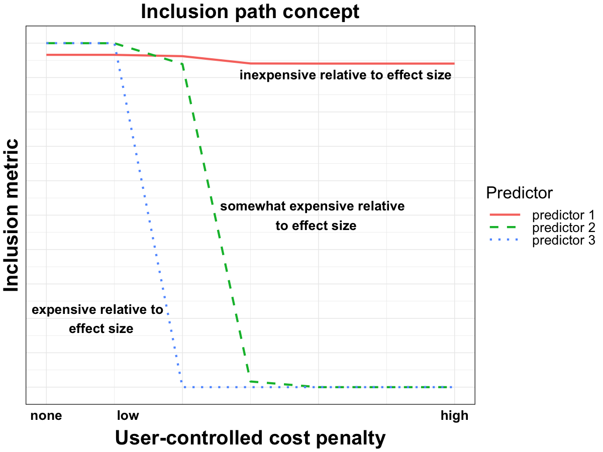
Figure 1: Diagram prefacing our proposed inclusion path. The practitioner controls cost penalization to accommodate a budget and uses the inclusion metric value to study how each predictor’s importance for modeling the outcome changes as cost is penalized differently.

Several methods based on decision theory have also been proposed to penalize for predictor costs. For example, Brown et al. (1999) developed a decision-theoretic approach for multivariate linear regression which added to a quadratic loss function a terminal cost function representing the cost of keeping a particular subset of candidate predictors. Fouskakis and Draper (2008) proposed a decision-theoretic approach for binary outcome generalized linear models that appended a data collection utility component based on marginal predictor costs to the expected utility function, and they applied this utility function to several stochastic optimization algorithms. Recently, Miyawaki and MacEachern (2022) added a cost function to the traditional predictive loss (Lindley, 1968) and apply Bayesian model averaging (BMA) first over purchased predictors and then by marginalizing over potential unpurchased predictors via MCMC. They find that the latter approach performs better than standard BMA but introduces additional sensitivity in prior specification and requires further subjective prior information and assumptions, such as the joint distribution of unobserved predictors. In another MCMC-based approach, Fouskakis et al. (2009b) used a reversible jump MCMC to search the model space constrained to models whose total predictor costs fall below a threshold. Machine learning is another area that has seen some development of cost-penalized methods that may be adapted for medical applications (Elkan, 2001; Fan et al., 1999; Cohn et al., 1996; Settles, 2009; Bolón-Canedo et al., 2014; Kong et al., 2016; Ling et al., 2004; Zhou et al., 2016; Adams et al., 2016). In contrast, our method provides a single user-controlled tuning parameter to adjust the magnitude of cost penalization on candidate predictors to produce multiple cost-penalized analyses and produce probabilities for all candidate models and predictors.

The FND prior, which our proposed method extends, penalizes costly predictors relative to a minimum (baseline) cost, and Fouskakis et al. (2009a) used the prior to develop a cost-adjusted selection approach which results in a generalized version of BIC. Fouskakis et al. (2009a) developed cost-adjusted BIC to select among sickness indicators for predicting death within $30$ days due to pneumonia. Fouskakis et al. (2009a) compared their selection results to those in which a uniform prior is used for all predictors and models. The latter approach, which Fouskakis et al. (2009a) call a benefit-only analysis, as it ignores costs, selects a more costly model when applied to a set of $n=2,532$ pneumonia patients.

When applying the FND prior to other data sets, we have found that the FND prior can lead to selection of less costly models when predictor costs differ, but the cost penalization is not appropriate or sufficient for all sample sizes. In fact, at large sample sizes, the cost penalization imposed by the FND prior greatly diminishes, often causing the resulting cost-penalized model selection to closely resemble that of a standard benefit-only analysis. To establish this phenomenon, we calculated the Kullback-Leibler (KL) divergence, which measures the difference between two probability distributions, between the sets of posterior model probabilities for all candidate models produced by cost-penalized analysis with the FND prior and the benefit-only selection approach as sample size increases for several simulated data sets. Since we consider the case of linear logistic regression, for which there is no closed form integrated likelihood, we examine the KL divergence comparing posterior model probabilities from the two approaches empirically. We generated $10$ data sets of size $n=150$ with $p=9$ total candidate predictors with different costs as detailed in Section 3.1 and calculated the KL divergence between the two sets of posterior model probabilities produced by the benefit-only and FND selection approaches for each data set. Then, to imitate collection of additional data, we recursively added $300$ observations to the initial $10$ data sets, obtaining model selection results and calculating KL divergence between the posterior model probabilities produced by the two selection approaches for each new (larger) data set. Figure 2 plots the KL divergence between the posterior model probabilities produced by the two approaches as sample size increases for the $10$ collections of data sets increasing in size.

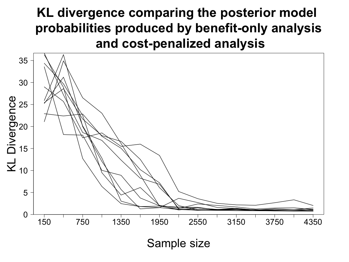
Figure 2: KL divergence calculated between the sets of posterior model probabilities produced using the FND prior and benefit-only model selection for $10$ collections of data sets where 300 observations were recursively added to 10 initial data sets of size $n=150$. These data were generated from the linear logistic regression setting considered by Fouskakis et al. (2009a). See Section 3.1 for more details. The KL divergence between the posterior model probabilities produced by the two approaches decreases as the sample size grows for all $10$ collections of data sets increasing in size, with 7 of the $10$ near $0$ by $n=2500$, indicating that as sample size increases, the impact of the cost penalty on the model selection is reduced.

Figure 2 shows that the KL divergence value between the posterior model probabilities for all candidate models produced by the cost-penalized and benefit-only methods approaches $0$ as the sample size increases. Thus, larger sample sizes lead cost-penalized Bayesian model selection using the FND prior to select a model with structure and cost similar to that of a benefit-only approach. In many cases, this occurrence may not be ideal, since the user adopted the FND prior to control/reduce cost from the selected predictors. But when the sample size of the available data is large, the cost-penalizing ability of the FND prior diminishes and the approach recommends the costly benefit-only model the user was hoping to avoid. Ironically, collecting more observations, which often inherently increases medical study costs, can dilute or cancel out the penalization for costly predictors. This phenomenon may lead practitioners and medical researchers to plan for studies that are more expensive than necessary. In this paper we extend the FND prior by proposing simple functions for adjusting the cost penalization according to a tuning parameter. These functions extend the useful FND prior and maintain the property of invariance to cost conversions, making them widely applicable. Our inclusion path approach highlights the change in posterior inclusion probabilities for individual candidate predictors at different levels of the cost penalization according to the functions we suggest. The inclusion path weighs the modeling ability against the cost of the predictors. We demonstrate the utility of our adjusted cost penalization and inclusion path approach first with simulated data and then a data set collected at a medical clinic on Cleveland, Ohio, where the response is the presence of heart disease. There are $13$ candidate predictors relevant to diagnosing heart disease available for each patient, with widely varying costs (Detrano et al., 1989). A benefit-only approach selects many costly predictors that do not appreciably improve modeling of heart disease. We show that our adjusted cost penalization can be used to select models with reduced costs per patient, which can help to meet hospital or insurance budgets, while still retaining cost-effective predictors for physicians to diagnose a critical condition like heart disease. Our functions that adjust the cost penalization extend the utility of the FND prior. The resulting inclusion path plots the changing impact of candidate predictors where the practitioner now has input over the magnitude of cost penalization.

The remainder of this paper is organized as follows. Section 2 introduces cost-penalized Bayesian model selection, describes the FND prior, details our functions and properties for adjusting the cost penalization on predictors, outlines our inclusion path approach, and explains the setup for our simulated data. Section 3 demonstrates the utility of the FND prior and presents our adjusted cost penalization and inclusion path approach, first using simulated data and then when applied to the Cleveland heart disease data. All selection results for our method are compared to results produced by the FND prior. Section 4 summarizes the impact of our findings and outlines avenues for potential future research and applications in cost-penalized model selection.

2 Data and Methods

2.1 Bayesian model selection

We consider Bayesian model selection with the goal of penalizing candidate predictors based on their costs through a flexible class of model priors. Each candidate predictor has an associated cost. We use Bayesian model selection to obtain posterior model probabilities for each possible combination of predictors, with the goal being to select a subset of predictors that accurately classify the outcome while penalizing on the basis of the costs of those predictors. For $p$ candidate predictors, the corresponding model space is $\mathcal{M}=\{0,1\}^{p}=\{M_{1},M_{2}\ldots,M_{K}\}$, where $K=|\mathcal{M}|=2^{p}$ is the total number of candidate models. To compare two models, say $M_{1}$ and $M_{2}$, we may use the Bayes factor, $BF_{12}$, that is defined as the ratio of the two models’ integrated likelihoods:

$$BF_{12}=\frac{p(\textbf{Y}|M_{1})}{p(\textbf{Y}|M_{2})}.$$ (1)

Then the posterior model probability of a single model $M_{\ell}$ in the model space can be found using Bayes’ Rule:

$$P(M_{\ell}|\textbf{Y})=\frac{p(\textbf{Y}|M_{\ell})P(M_{\ell})}{\sum_{k=1}^{K}p(\textbf{Y}|M_{k})P(M_{k})}=\bigg{(}\sum_{k=1}^{K}BF_{k\ell}\times\frac{P(M_{k})}{P(M_{\ell})}\bigg{)}^{-1},$$ (2)

where $P(M_{k})$ is the prior model probability for model $M_{k}$. We now describe the FND prior in Section 2.2.

2.2 Cost-penalizing model selection

Fouskakis et al. (2009a) developed the FND prior for variable selection for the linear logistic regression setting, with the goal of optimizing selection of sickness indicators for improving quality of health care assessments while penalizing expensive candidate predictors. Their motivating data set from the RAND Corporation was used to select from a list of $83$ sickness indicators to model patient deaths within $30$ days of admission due to pneumonia, where costs were measured as the time required to observe/record predictors for each patient (Keeler et al., 1990). In particular, both the benefit-only analysis and cost-penalized analysis using the FND prior selected $13$ predictors from $83$ total candidate predictors, but the total cost of the two sets of selected predictors were 22.5 and 9.5 (in minutes), respectively, resulting in a cost reduction of more than 50%. Their approach is invariant to cost conversions, devised a penalty related to BIC relative to a baseline cost, and can be used to reproduce the traditional BIC when all predictor costs are equal. Further, by using expressions based on posterior model odds, Fouskakis et al. (2009a) were able to produce posterior model probabilities from a generalized cost-adjusted version of the BIC, which shares many similarities with the approximations and behaviors of the traditional BIC.

Following Fouskakis et al. (2009a), we consider the linear logistic regression setting in this paper, later applying it to the binary diagnosis of heart disease. For convenience, we use the notation of Fouskakis et al. (2009a) for indicator functions and predictor costs. We use a linear logistic regression model where $Y_{i}\in\{0,1\}$ and $X_{ij}$ denotes the $j{\color[rgb]{0,0,0}{}^{th}}$ predictor for observation $i$, where $i=1,\ldots,n$ and $j=0,\ldots,p$. Let $\gamma_{j}$ be an indicator that is equal to $1$ if predictor $X_{j}$ is included in the model and $0$ if it is not. Then $\boldsymbol{\gamma}$ is a length $p$ vector of $0$’s and $1$’s indicating whether each of the $p$ predictors are in the model or not. Note that the intercept is included in every model so $X_{i0}=1$ and $\gamma_{0}=1$ for all models. Then the Bayesian modeling framework is

$$\begin{split}&(Y_{i}|\boldsymbol{\gamma})\overset{\text{indep}}{\sim}\text{Bernoulli}[p_{i}(\boldsymbol{\gamma})],\\ &\eta_{i}(\boldsymbol{\gamma})=\log\Big{[}\frac{p_{i}(\boldsymbol{\gamma})}{1-p_{i}(\boldsymbol{\gamma})}\Big{]}=\sum_{j=0}^{p}\beta_{j}\gamma_{j}X_{ij},\\ &\eta(\boldsymbol{\gamma})=\boldsymbol{X}\text{diag}(\boldsymbol{\gamma})\beta=\boldsymbol{X}_{\boldsymbol{\gamma}}\boldsymbol{\beta}_{\boldsymbol{\gamma}},\end{split}$$ (3)

where $\boldsymbol{X}_{\boldsymbol{\gamma}}$ and $\boldsymbol{\beta}_{\boldsymbol{\gamma}}$ are the design matrix and vector of regression coefficients for the specific model with predictors in $\boldsymbol{\gamma}$. For the vector of regression coefficients $\boldsymbol{\beta}_{\boldsymbol{\gamma}}$, we assign a Gaussian prior distribution $\pi(\boldsymbol{\beta}_{\boldsymbol{\gamma}})$ with form $N(\boldsymbol{\mu}_{\boldsymbol{\gamma}},\Sigma_{\boldsymbol{\gamma}})$. We assume the same prior for $\boldsymbol{\beta}_{\boldsymbol{\gamma}}$ as derived by Fouskakis et al. (2009a), so a prior $\boldsymbol{\beta}_{\boldsymbol{\gamma}}$ is distributed as:

$$\boldsymbol{\beta}_{\boldsymbol{\gamma}}|\boldsymbol{\gamma}\sim N(\boldsymbol{0},4n(\boldsymbol{X}_{\boldsymbol{\gamma}}^{T}\boldsymbol{X}_{\boldsymbol{\gamma}})^{-1}).$$ (4)

The cost-penalized prior by Fouskakis et al. (2009a) for a single $\gamma_{j}$ is proportional to:

$$P(\gamma_{j})\propto\exp\Big{[}-\frac{\gamma_{j}}{2}\Big{(}\frac{c_{j}}{c_{0}}-1\Big{)}\log n\Big{]},$$ (5)

where $c_{j}$ is the marginal cost per observation for predictor $X_{j}$ and $c_{0}=\text{min}\{c_{j},j=1,\ldots,p\}$ is defined as the baseline cost, corresponding to the cheapest (least expensive) candidate predictor. Then the FND prior for a particular model corresponding to $\boldsymbol{\gamma}$ follows as:

$$P(\boldsymbol{\gamma})=\exp\bigg{\{}-\frac{1}{2}\log n\sum_{j=1}^{p}\gamma_{j}\bigg{(}\frac{c_{j}}{c_{0}}-1\bigg{)}-\sum_{j=1}^{p}\log\big{[}n^{-\frac{1}{2}(\frac{c_{j}}{c_{0}}-1)}+1\big{]}\bigg{\}}.$$ (6)

A natural comparator to (6) is a uniform prior on the model space:

$$P(\boldsymbol{\gamma})=\frac{1}{2^{p}},$$ (7)

which produces the benefit-only selection when used with Equation (2). We use a Laplace approximation to approximate the integrated likelihoods with distribution (3) and prior (4), and we obtain posterior model probabilities for all models in $\mathcal{M}$ as in Equation (2).

We develop our inclusion path approach, presented in Section 2.4, using posterior inclusion probabilities for the candidate predictors. The posterior inclusion probability for predictor $X_{j}$ is obtained by adding up the posterior model probabilities from each model containing $X_{j}$, i.e. where $\gamma_{j}=1$:

$$P(\gamma_{j}=1|\textbf{Y})=\sum_{\boldsymbol{\gamma}_{k}\in\mathcal{M}|\gamma_{j}=1}P(\boldsymbol{\gamma}_{k}|\textbf{Y}).$$ (8)

Equation (6) uses the marginal cost $\{c_{j},j=1,\ldots p\}$ of each candidate predictor, which is the cost of collecting that predictor for a single observation. When adhering to an overall budget, the practitioner may also want to consider the total cost per observation or the total cost of the model. The total cost per observation is equal to the sum of the marginal cost of all predictors in the model, i.e. $\sum_{j=1}^{p}{\color[rgb]{0,0,0}c_{j}}\gamma_{j}$, and the total cost of the model for the given observations is $n\times\sum_{j=1}^{p}{\color[rgb]{0,0,0}c_{j}}\gamma_{j}$.

Note that our approach penalizes predictors based on their predetermined costs. Therefore, the resulting posterior probabilities that we discuss are cost-adjusted probabilities rather than probabilities in the traditional Bayesian sense of the true model. These cost-adjusted probabilities can be used to determine whether a model contains cost-effective or efficient predictors relative to other models when provided with the desired level of cost-penalization from the user, rather than being interpreted as the chance of a model being the true model. For the remainder of this paper, we refer to any posterior probabilities obtained under a cost penalty on the predictors as ‘cost-adjusted posterior probabilities’. The exception is the benefit-only model selection approach, which we show can be obtained by setting our proposed tuning parameter equal to 0, and which produces posterior probabilities that are not cost-adjusted.

2.3 Adjusted cost-penalizing functions

The cost penalization from the FND prior in Equation (6) increases with sample size, i.e., through the $\log(n)$ term. However, as demonstrated in Figure 2, the cost penalization does not always grow quickly enough with $n$, so the FND prior may not be sufficient for all data sets or budgets, particularly in the case of large sample sizes. We propose an extension of the FND prior that gives the practitioner more flexibility when penalizing predictors based on their costs a priori. One way to improve the flexibility of the FND prior is the ability to adjust the cost penalization rather than relying on a fixed penalization for every application with cost. If the cost of the model selected based on existing data exceeds a current or future budget, it would be crucial to be able to increase the cost penalization to find an effective but affordable model. For other data, it might be the case that the model selected using the FND prior does not provide the desired performance and then it may be crucial to decrease the cost penalization to allow for selection of additional predictors that would improve the model’s overall performance while still penalizing for high costs, just to a lesser extent. To give practitioners more control over the FND prior so that it may scale to their problem, we propose functions of the cost ratio $c_{j}/c_{0}$ according to a tuning parameter $b$. These functions change the magnitude of cost penalization in the FND prior.

We propose functions $g(c_{j}/c_{0},{\color[rgb]{0,0,0}b})$ to adjust the cost ratio according to tuning parameter $b$ that satisfy the following properties:

1. $b=0$ implies $g(c_{j}/c_{0},{\color[rgb]{0,0,0}b})=1$ for all $j=1,\ldots,p$, reducing the prior to the uniform model prior (7) and resulting in a benefit-only model selection.

2. $b=1$ makes $g(c_{j}/c_{0},{\color[rgb]{0,0,0}b})$ equal to $c_{j}/c_{0}$ and reproduces the FND prior as seen in Equation (6).

3. When $b>1$, $g(c_{j}/c_{0},{\color[rgb]{0,0,0}b})$ penalizes predictors with costs $c_{j}>c_{0}$ more highly than the FND prior in (6). When $0<b<1$, $g(c_{j}/c_{0},{\color[rgb]{0,0,0}b})$ penalizes predictors with costs $c_{j}>c_{0}$ less than the FND prior but more than a benefit-only analysis. Higher values of $b$ increase $g(c_{j}/c_{0},{\color[rgb]{0,0,0}b})$ and the resulting cost penalization, leading to lower cost-adjusted prior inclusion probabilities for predictors with costs above the baseline.

4. When $c_{j}=c_{0}$, the $j{\color[rgb]{0,0,0}{}^{th}}$ candidate predictor cost is the same as the baseline cost. Changing $b$ does not introduce/increase penalization on any of the predictors with baseline cost.

We propose to use a model prior of the form (6) where the cost ratio $c_{j}/c_{0}$ is replaced with the cost ratio function $g(c_{j}/c_{0},b)$, as follows

$$P(\boldsymbol{\gamma})=\exp\bigg{\{}-\frac{1}{2}\log n\sum_{j=1}^{p}\gamma_{j}\bigg{(}g\bigg{(}\frac{c_{j}}{c_{0}},b\bigg{)}-1\bigg{)}-\sum_{j=1}^{p}\log\big{[}n^{-\frac{1}{2}\big{(}g\big{(}\frac{c_{j}}{c_{0}},b\big{)}-1\big{)}}+1\big{]}\bigg{\}}.$$ (9)

In general, monotone functions of the cost ratio and tuning parameter $b$ are well-suited for our cost-adjusted model prior and proposed inclusion path. Here we study an exponential function of the cost ratio according to the tuning parameter. Another sensible choice is a linear function of the cost ratio, which we describe in the Supplementary Material.

For a given value of the tuning parameter $b$, the exponential function of the cost ratio for predictor $X_{j}$ is

$$g\bigg{(}\frac{c_{j}}{c_{0}},b\bigg{)}=\bigg{(}\frac{c_{j}}{c_{0}}\bigg{)}^{b},$$ (10)

which satisfies properties (a)-(d). We call the prior that uses the exponential function of the cost ratio function in (10) the exponential cost prior (ECP). That is, the ECP is model prior with form (9) where $g(c_{j}/c_{0},b)=(c_{j}/c_{0})^{b}$.

2.4 Inclusion paths

Using the ECP and varying $b$, we create an inclusion path for each candidate predictor. To do this, we compute and plot cost-adjusted posterior inclusion probabilities for each of the candidate predictors across multiple values of $b$. See the Supplementary Material for detailed steps for constructing the inclusion path. The inclusion path visualizes a probabilistic way to learn the order in which the candidate predictors would be chosen or discarded, e.g. according to some threshold, if a different magnitude of cost penalization is used. The costs $\{c_{j},j=1,\ldots p\}$ remain unchanged; $g(c_{j}/c_{0},{\color[rgb]{0,0,0}b})$ changes how heavily candidate predictors with larger costs are penalized a priori. Our inclusion path technique is inspired by the interpretable path diagrams like LASSO and ridge (Tibshirani, 1996; Hoerl and Kennard, 1970). From the plot of inclusion paths, the practitioner can all at once study candidate predictors’ posterior inclusion probabilities for the benefit-only analysis and cost-adjusted posterior inclusion probabilities for the FND prior and a wide range of the ECP with differing $b$ values. This is because we formulated the ECP to satisfy properties (a)-(d) so that the established uniform priors and the FND prior can be easily recreated from the ECP.

3 Results

3.1 Simulation study settings

To study the model selection behavior resulting from the FND prior and ECP, consider a simulated data set of size $n=150$ with form (3) and vector of regression coefficients

$$\boldsymbol{\beta}=(1,0,0,0,0.5,0.5,0.5,0.8,0.8,0.8)^{T},$$ (11)

and corresponding cost vector

$$\boldsymbol{c}=(1,3,9,1,3,9,1,3,9),$$ (12)

representing predictors with all combinations of null, smaller, and larger effect sizes and baseline, cheap, and expensive costs. The predictors $X_{1},\ldots,X_{9}$ are generated independently from a $N(0,1)$ distribution. The vector of regression coefficients (11) and predictor costs (12) were also used to generate the $10$ series of data sets increasing in size used to calculate KL divergence values between the the posterior model probabilities (benefit-only and cost-adjusted) resulting from the benefit-only analysis and the FND prior in Section 1.

In practice, medical costs can be measured and recorded according to money, time, labor, and many other quantities. The FND prior and our ECP extension are both invariant to cost units/conversions since the cost penalizations are expressed relative to the baseline cost. Often the goal may be to focus on efficiency rather than minimizing an overall cost, as this may better serve a patient or hospital operations. Therefore, we choose to consider the costs for our simulated data as the time in minutes required to collect each predictor for one individual. Thus, our simulation setting has $512$ candidate models with costs ranging from $0$ minutes (corresponding to the intercept-only) and $39$ minutes per observation. Section 3 presents selection results for data generated as above using Bayesian model selection as described in Section 2 with uniform priors, the FND prior, and the ECP applied to the model space.

3.2 Simulation results using FND prior

Consider a data set of size $n=150$ generated as described in Section 3.1. Table 1 highlights the difference between the selection results from a benefit-only approach and selection using the FND prior. For the following sections, we will describe both MAP model, i.e. the model selected using the maximum posterior model probability (benefit-only or cost-adjusted) and the median probability model, which consists of predictors’ whose posterior inclusion probability (benefit-only or cost-adjusted) is at least 0.5 (Barbieri and Berger, 2004). For the data sets described in Tables 1 and 2, the MAP model and the median probability model are the same. We can see from Table 1 that the benefit-only model selection approach selects the model containing $X_{5}$ through $X_{9}$, i.e. the cheap and expensive predictors with smaller effect size and all three of the predictors that have the larger effect size. This model has a total cost of 25 minutes per observation. The posterior model probability for this benefit-only model is 0.332, moving off of the prior probability of 0.002, and the corresponding C-statistic, defined as the area under the receiver operating characteristic (ROC) curve, is 0.84. Meanwhile, model selection using the FND prior on the model space selects the model with the following predictors: $X_{7}$ (baseline predictor with larger effect size) and $X_{8}$ (cheap predictor with larger effect size), for a total cost of 4 minutes per observation, a $84\%$ reduction in cost from the benefit-only model. The cost-adjusted posterior model probability for this model is 0.491, moving off of its prior probability of 0.0008, and the corresponding C-statistic is 0.782. We can see that the FND prior leads to a remarkable reduction in the cost per observation for its selected model and successfully prioritizes predictors with larger effect sizes while it considers their costs, while incurring modest loss in accuracy as measured by the C-statistic.

Benefit-only selection	FND selection
$n=150$	$n=150$
Predictor Effect Cost Cost size level (mins.) $X_{1}$ null baseline 1 $X_{2}$ null cheap 3 $X_{3}$ null expensive 9 $X_{4}$ smaller baseline 1 $X_{5}$ smaller cheap 3 $X_{6}$ smaller expensive 9 $X_{7}$ larger baseline 1 $X_{8}$ larger cheap 3 $X_{9}$ larger expensive 9 25/obs	Predictor Effect Cost Cost size level (mins.) $X_{1}$ null baseline 1 $X_{2}$ null cheap 3 $X_{3}$ null expensive 9 $X_{4}$ smaller baseline 1 $X_{5}$ smaller cheap 3 $X_{6}$ smaller expensive 9 $X_{7}$ larger baseline 1 $X_{8}$ larger cheap 3 $X_{9}$ larger expensive 9 4/obs

Table 1: Candidate predictors and their corresponding effect sizes and costs. Rows colored in orange   are the predictors selected by (left) the benefit-only analysis and (right) selection using the FND prior for a data set of size $n=150$. At this small sample size, the benefit-only model costs more than $4$ times the model selected using the FND prior.

However, as is often the case with Bayesian methods, the influence of the prior is reduced as the sample size increases. In this case, the cost penalization from the FND prior diminishes as the sample size increases. As a result, for large sample sizes, the cost-penalized selection using the FND prior more closely resembles the benefit-only model selection. To view the changing impact of the cost penalization on selection as sample size increases, consider a similar data set of size $n=600$. To mimic collection of additional data, we added $450$ new data points simulated from the settings in (11) and (12) to the set of $n=150$ studied in Table 1, resulting in a data set of size $n=600$. For this larger data set we again performed model selection first using a benefit-only analysis with uniform priors (7) and then using cost-penalized Bayesian model selection with the FND prior on the model space. Both selection approaches choose the same model with all $6$ predictors with non-null effect sizes, with a total cost of 26 minutes per observation. Table 2 highlights the identical selection results from these two analyses for the size $n=600$ data set. The C-statistic for the model containing every non-null predictor is 0.865, with posterior model probability equal to 0.594 from the benefit-only analysis (model prior 0.002) and cost-adjusted posterior model probability equal to 0.927 using the FND prior for selection (model prior 2e-29).

With the two selection results being identical, we can see that the cost penalization provided by the FND prior was ineffective after the addition of only $450$ more observations. Thus, the reward for incurring the expense of additional data collection is to recommend a more expensive (or inefficient) model, the same as when no cost penalty is used. If looking to decide which predictors to collect, for example, in a future study, a practitioner may use the FND prior and come to very different decisions based on the size of their existing data, by only a few hundred observations. This points to a need to be able to adjust the cost penalization to provide cost-effective model selection for each medical application at hand. Section 3.3 demonstrates how the ECP can be used with our inclusion path approach to adjust the cost penalization so that it can be maintained at different sample sizes.

Benefit-only selection	FND selection
$n=600$	$n=600$
Predictor Effect Cost Cost size level (mins.) $X_{1}$ null baseline 1 $X_{2}$ null cheap 3 $X_{3}$ null expensive 9 $X_{4}$ smaller baseline 1 $X_{5}$ smaller cheap 3 $X_{6}$ smaller expensive 9 $X_{7}$ larger baseline 1 $X_{8}$ larger cheap 3 $X_{9}$ larger expensive 9 26/obs	predictor Effect Cost Cost size level (mins.) $X_{1}$ null baseline 1 $X_{2}$ null cheap 3 $X_{3}$ null expensive 9 $X_{4}$ smaller baseline 1 $X_{5}$ smaller cheap 3 $X_{6}$ smaller expensive 9 $X_{7}$ larger baseline 1 $X_{8}$ larger cheap 3 $X_{9}$ larger expensive 9 26/obs

Table 2: Candidate predictors and their corresponding effect sizes and costs. Rows colored in orange   are the predictors selected by (left) the benefit-only analysis and (right) cost-penalized selection using the FND prior for a data set of size $n=600$. After the addition of only $450$ more observations to the data set studied in Table 1, the benefit-only selection and Bayesian model selection using the FND prior choose the model with the same predictors and cost per observation, thus nullifying the default cost penalization from the FND prior.

3.3 Inclusion paths using adjusted cost penalization

Visualizing the effect of the tuning parameter $b$ enables the practitioner to see the change in all the predictors’ importance in the posterior for a range of cost penalizations. This forms the basis for our proposed inclusion path. Here, we demonstrate the proposed inclusion path approach with the ECP assigned to the model space. Consider a data set of size $n=450$, where the impact of the FND prior begins to diminish, simulated as described in Section 3.1. A similar example with correlated predictors appears in the Supplementary Material. We apply the ECP with cost ratio function (10) and a range of values for the tuning parameter $b$. We apply each of the resulting ECP model priors to the model space and obtain posterior inclusion probabilities (benefit-only or cost-adjusted) for each of the $9$ candidate predictors. Then we create an inclusion path by plotting the posterior inclusion probabilities (benefit-only or cost-adjusted) as a function of tuning parameter $b$. Figure 3(a) plots the inclusion path for each combination of candidate predictor cost and effect size when the ECP is used to adjust the amount of cost penalization.

From Figure 3(a), the posterior inclusion probabilities for $8$ of the $9$ predictors decrease as the cost penalization is increased via larger values of $b$. The predictor with the larger effect size and baseline cost maintains a posterior inclusion probability (benefit-only or cost-adjusted) at $1$ across all values of $b$, as it is not penalized a priori by the FND or ECP priors, according to property (d) from Section 2.3. The posterior inclusion probabilities for the cheap and expensive null predictors are $0.09$ and $0.25$, respectively, in the benefit-only analysis corresponding to $b=0$. The values of $0<b<1$ introduce cost penalization that is less severe than that from the FND prior but higher than the (nonexistent) cost penalization from the benefit-only analysis. For example, the cost-adjusted posterior inclusion probabilities for the cheap and expensive null predictors drop to $0.04$ and $0.06$ when $b=0.2$ is used with the ECP. Then the null predictor with expensive cost has $0$ cost-adjusted posterior inclusion probability for $b\geq 0.7$. Thus, even slightly penalizing these null predictors for having costs above the baseline helps to move their inclusion probabilities to $0$. For $b=1$ (the FND approach), the null predictor with cheap cost has cost-adjusted posterior inclusion probability $0.0002$, which decreases to $0$ for $b\geq 1.1$. The posterior inclusion probability of the null predictor with baseline cost is $0.12$ in the benefit-only analysis and the cost-adjusted posterior inclusion probability equals $0.05$ for $b\geq 3.5$, as this predictor has a null effect but is not penalized by any variation of the ECP. When determining which predictors are selected with each variation of the ECP, we can consider comparing the cost-adjusted posterior inclusion probabilities for the remaining non-null predictors to a threshold, e.g. $0.5$ as in the median probability model (Barbieri and Berger, 2004). The inclusion path allows us to see which predictors’ cost-adjusted inclusion probabilities meet the desired threshold for the different versions of cost-penalized selection at one time. For example, in the benefit-only analysis, which corresponds to the ECP with $b=0$, every one of the $6$ non-null predictors have posterior inclusion probabilities beyond the $0.5$ threshold under consideration. Using the FND prior, which corresponds to the ECP with $b=1$, the cost-adjusted posterior inclusion probabilities for all non-null predictors except for the expensive one with smaller effect size exceed the $0.5$ threshold. Figure 3 indicates that the cost-adjusted posterior inclusion probabilities fall below 0.5 at b = 1, 1.1, 1.5, and 1.8 for these predictors in the following order: expensive with smaller effect size, expensive with larger effect size, cheap with smaller effect size, and cheap with larger effect size.

The practitioner may choose a different threshold for the posterior inclusion probabilities (benefit-only or cost-adjusted) to suit their application. The goal of the inclusion path is to provide a way to select the best model that conforms to the practitioner’s budget by deciding which predictors to invest in. We use $0.5$ for illustration here.

The cost-adjusted posterior inclusion probabilities for this data set decrease with $b$ first according to cost and then by effect size. We found this trend to be true for this particular data set when a linear function of the cost ratio according to $b$ is used as well; see the Supplementary Material. Now imagine that the practitioner is planning a study and wishes to refrain from collecting some of the predictors, either to lower the overall cost or to be able to record more total observations. If the cost per observation for the benefit-only model here is too high, the practitioner might consider dropping/excluding predictors in an order first according to cost and then according to effect size, as indicated by the paths in Figure 3(a). A visual such as that in Figures 3(a) is important because it enables the practitioner to see how the different levels of cost penalization affect the posterior inclusion probabilities of individual predictors while also accounting for their effect sizes.

Figure 3(b) plots the cost of the selected model for each value of $b$ used to create the inclusion path in Figure 3(a). For this data set, the MAP model and median probability model are the same for all values of $b$. We can see that the cost of the selected model drops each time a predictor is no longer in the model, e.g. inclusion falls below 0.5. Figure 3(c) plots the accuracy in the form of the C-statistic of the selected model for each value of $b$. Similar to the cost in Figure 3(b), the C-statistic drops each time a predictor leaves the selected model as a result of a higher cost penalty. A practitioner, patient, or other stakeholder may use Figures 3(b) and 3(c) in conjunction with the inclusion path so they may keep any necessary budget, or desired efficiency or accuracy in mind when selecting cost-effective predictors.

(a)

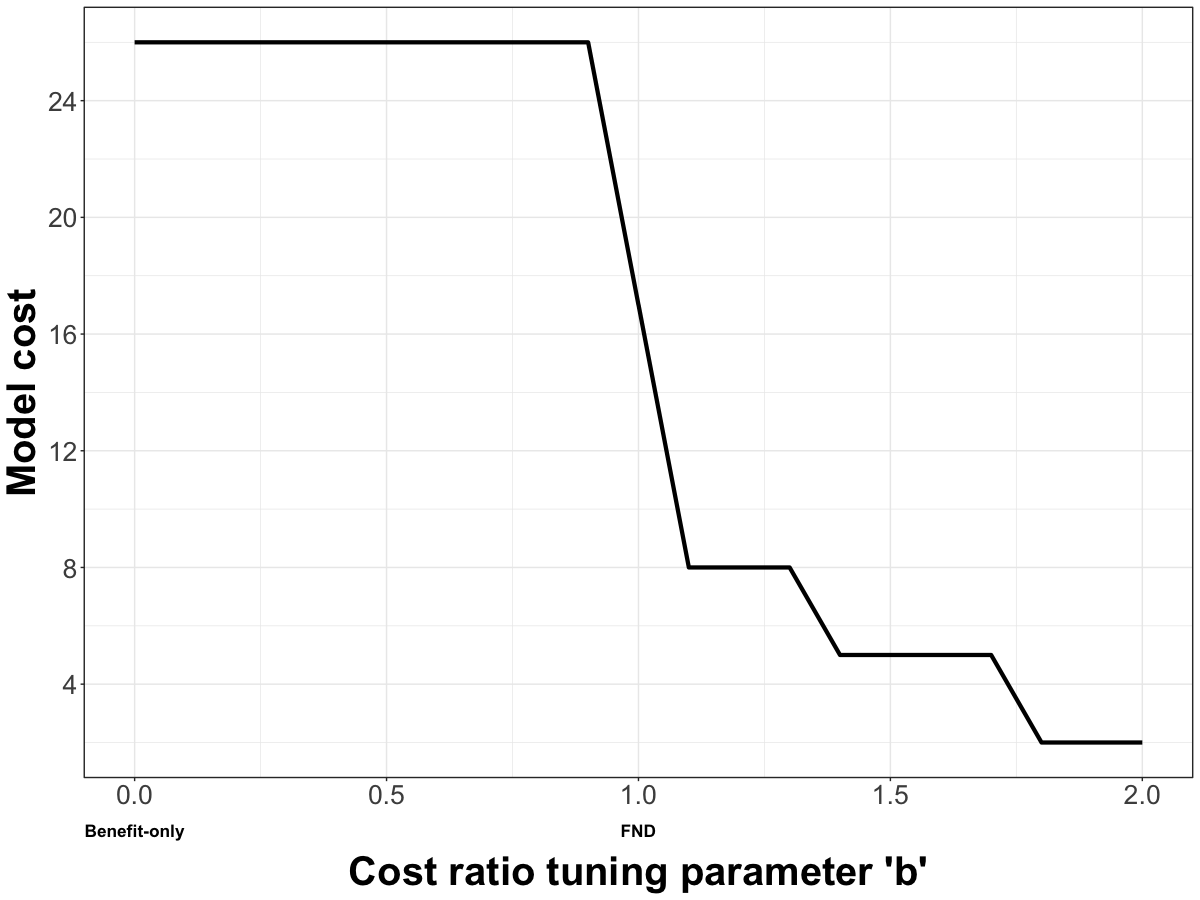
(b)

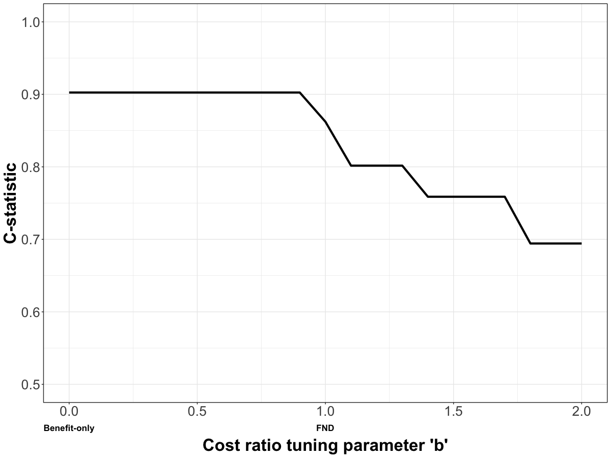
(c)

Figure 3: (a) Inclusion paths for each of the $9$ predictors with baseline, cheap, and expensive costs and null, smaller, and larger effect sizes for the $n=450$ data set, (b) the cost of the selected model (MAP and median probability models are the same for this data set), and (c) the C-statistic of the selected model. Model selection was performed using the ECP and tuning parameter values $b$ from 0 and 2 in increments of 0.1. Values of $b$ above $2$ are not shown here because there is no further change in the posterior inclusion probabilities or selected models.

3.4 Case study: selecting cost-effective predictors to model diagnosis of heart disease

We apply our adjusted cost-penalizing model selection to a data set of clinical test results originally from Detrano et al. (1989). The data consists of the medical records of $n=297$ patients collected at the Cleveland Clinic Foundation in 1988. We use these data for illustration because diagnosis of medical conditions such as heart disease is an important classification problem and the data are available along with the financial cost of each candidate predictor. We obtained these data from the UCI Machine Learning Repository. The response is a binary variable that indicates the presence of heart disease in each patient; $Y_{i}=1$ if the patient has heart disease and $Y_{i}=0$ if the patient does not have heart disease, where $i=1,\ldots,n$. There are $13$ candidate predictors. A summary of numeric candidate predictors appears in Table 3 and categorical candidate predictors are summarized in Table 4. Thus, there is a total of 8,192 models in the model space $\mathcal{M}$. Each predictor has an associated cost per patient, listed in the third column of Tables 3 and 4. The costs of the individual predictors range from $\$1.00$ to $\$102.90$, so the cost per observation ranges from $\$0.00$ (intercept-only) to $\$600.57$ for all 13 predictors per patient. Costs listed in Tables 3 and 4 are per patient and are specified in Canadian dollars, based on information from the Ontario Health Insurance Program.

Predictor	Description	Cost	Mean	St.	Odds
name		(in $)		dev.	ratio*
age	Patient age (years)	1	54.54	9.05	1.61
resting BP	Resting blood pressure (mm Hg)	1	131.69	17.76	1.37
cholesterol	Serum cholestoral (mg/dl)	7.27	247.35	51.99	1.18
heart rate	Maximum heart rate achieved	102.90	149.60	22.94	0.36
ST depression	ST depression induced by exercise	87.30	1.06	1.17	2.91
	relative to rest

Table 3: Numeric candidate predictors for the Cleveland heart disease data. *The odds ratios are expressed in terms of an increase of one standard deviation in the predictor, and reflect the odds of the patient having a positive heart disease diagnosis.

Predictor	Description	Cost	Values	Percent	Odds
name		(in $)		observed	ratio**
sex	Patient sex	1	0-Female	32.3%	-
			1-Male	67.7%	3.57
blood	Fasting blood	5.20	0-False	85.5%	-
sugar	sugar		1-True	14.5%	1.02
exercise	Exercise-induced	87.30	0-No	67.3%	-
angina	angina		1-Yes	32.7%	7.00
chest	Chest pain	1	1- Typical angina	7.7%	-
pain	type		2-Atypical angina	16.5%	0.51
			3-Non-anginal pain	27.9%	0.63
			4-Asymptomatic	47.8%	6.04
EKG	Resting	15.50	0-Normal	49.5%	-
	electrocardiogram		1-ST-T wave abnormality	1.3%	5.02
	results		2-Probable/definite left	49.2%	1.97
peak ST	Slope of the	87.30	1-Upsloping	46.8%	-
segment	peak exercise		2-Flat	46.1%	5.31
	ST segment		3-Downsloping	7.1%	3.81
major	Major vessels	100.90	0	58.6%	-
vessels	colored by		1	21.9%	6.01
	flourosopy		2	12.8%	12.70
			3	6.7%	16.24
defect	Type of heart	102.90	3-Normal defect	55.2%	-
type	defect		6-Fixed defect	6.1%	6.87
			7-Reversible defect	38.7%	11.19

Table 4: Categorical candidate predictors for the Cleveland heart disease data. **Odds ratios measure the shift in multiplicative odds from the reference category (denoted by -) of having a positive heart disease diagnosis.

We performed Bayesian model selection using the heart disease data, applying a benefit-only approach and cost-penalized model selection as described in Section 2 with the FND and ECP priors assigned to the model space. Benefit-only model selection with uniform priors (7) on the model space selects the model with the following predictors: sex, chest pain, resting BP, ST depression, peak ST segment, major vessels, and defect type with corresponding posterior model probability $0.072$, up from a prior model probability equal to 0.000122 and with a total cost of $\$381.40$ per patient. Model selection using the FND prior on the model space selects the model with the four baseline predictors (sex, age, chest pain, and resting BP), with corresponding cost-adjusted posterior model probability equal to 0.5. This model that contains only baseline predictors has prior model probability equal to $0.063$ using the FND prior, and a cost equal to $\$4.00$ per patient. While cost-penalized selection with the FND prior leads to a less costly model that is only $2.3\%$ of the cost of the benefit-only model, this model performs worse than more costly models in terms of classification. Figure 5 displays ROC curves and corresponding costs for models selected using different values of $b$ with ECP; the values of $b$ listed correspond to the median probability model. Detection of a health condition such as heart disease is critical for doctors to be able to provide effective treatment and advice to affected patients. The cost $\$4.00$ model might not have acceptable false positive rates for the hospital to trust the diagnosis, and thus it is desirable to be able to adjust the cost penalization, particularly between $0<b<1$, for these data. Our method is key for striking a balance between the benefit-only approach and the FND approach, by furnishing a spectrum of cost penalization choices. The C-statistics for the models considered in Figure 5 are 0.934, 0.931, 0.917, 0.887, and 0.849 for the median probability models from the ECP with $b=$ 0, 0.15, 0.25, 0.35, and 1, respectively. To assess out-of-sample predictive accuracy, we also calculated a leave-one-out C-statistic for each model by obtaining predicted probabilities for each observation based on regression coefficient estimates obtained without that observation; these values were 0.912, 0.909, 0.896, 0.867, and 0.833, respectively. We can see that penalizing based on predictor costs (e.g. with $b=0.15$) can lead to great cost reduction with very little loss in performance compared to the benefit-only model. Perhaps surprisingly, the model with cost equal to only $\$4.00$ per patient has a C-statistic of 0.849, which indicates that it might have some utility in a triage scenario. However, our method provides the ability for practitioners to see which predictors can supplement the model to improve diagnosis beyond easily-obtained predictors like age and sex and a subjective pain rating from the patient.

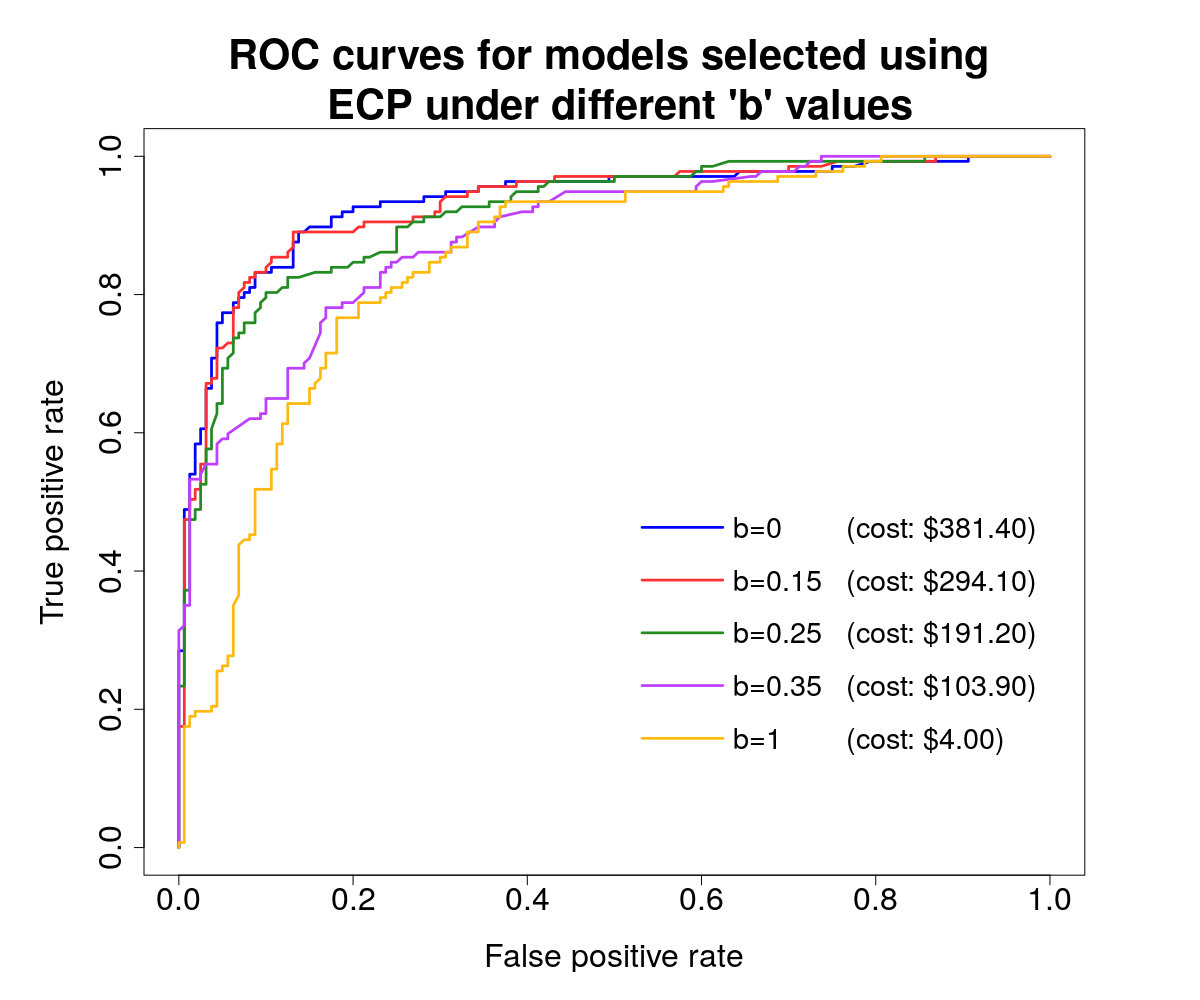
Figure 4:

Figure 5: ROC curves for median probability models for the Cleveland heart disease data using Bayesian model selection with the ECP model prior and different values of tuning parameter $b$. The median probability and the MAP model for $b\geq 0.45$ is always the cost $4.00 model containing only the four baseline predictors. $b=1$ corresponds to the FND model prior.

To study the individual candidate predictors for diagnosing heart disease, we applied our inclusion path approach with adjusted cost penalization to the heart disease data from Detrano et al. (1989). Figure 6(a) contains the inclusion path using the ECP with tuning parameter values of $b$ between 0 and 0.6. The lines corresponding to each predictor’s inclusion path are color-coded such that lines corresponding to predictors with the same cost are the same color; darker shades of red correspond to more costly predictors, and then line types differ between distinct predictors that have the same cost. Values of $b$ above $0.6$ are not shown here, as the cost-adjusted posterior inclusion probabilities do not change for $b>0.6$ for these data, and the cost $\$4.00$ model containing only the baseline predictors is selected with highest posterior model probability for all $b>0.5$.

From Figure 6(a) we can see that the posterior inclusion probabilities for the baseline predictors sex and chest pain are high for the benefit-only analysis as well as all cost-penalized analyses, with the cost-adjusted posterior inclusion probabilities being equal to $1$ for all values of $b\geq 0.4$. The posterior inclusion probability for baseline predictor age is only $0.09$ in the benefit-only analysis; then the cost-adjusted posterior inclusion probability increases to $0.64$ at $b=0.4$ and reaches and remains at $0.96$ for $b\geq 0.5$. The final baseline predictor, resting BP, has posterior model probability equal to $0.59$ in the benefit-only analysis. Its cost-adjusted posterior inclusion probability increases with $b$ until $b=0.3$, then decreasing to $0.53$ for $b\geq 0.1$, always remaining above a $0.5$ probability threshold. Predictors heart rate, exercise angina, cholesterol, EKG, and blood sugar have posterior inclusion probabilities below $0.5$ in the benefit-only analysis; cost-adjusted posterior inclusion probabilities for these five predictors all move towards $0$ as the cost penalty increases, indicating that these predictors would not be chosen based on a benefit-only or a cost-penalized analysis unless a lower threshold is used. The posterior inclusion probabilities for ST depression and defect type are equal to $0.75$ and $0.96$, respectively, in the benefit-only analysis. The cost-adjusted posterior inclusion probabilities for both ST depression and defect type continue to decrease towards 0 as $b$ increases. Finally, the peak ST segment predictor has posterior inclusion probability 0.64 for $b=0$; its cost-adjusted posterior inclusion probability fluctuates until $b=0.3$ and then decreases towards 0.

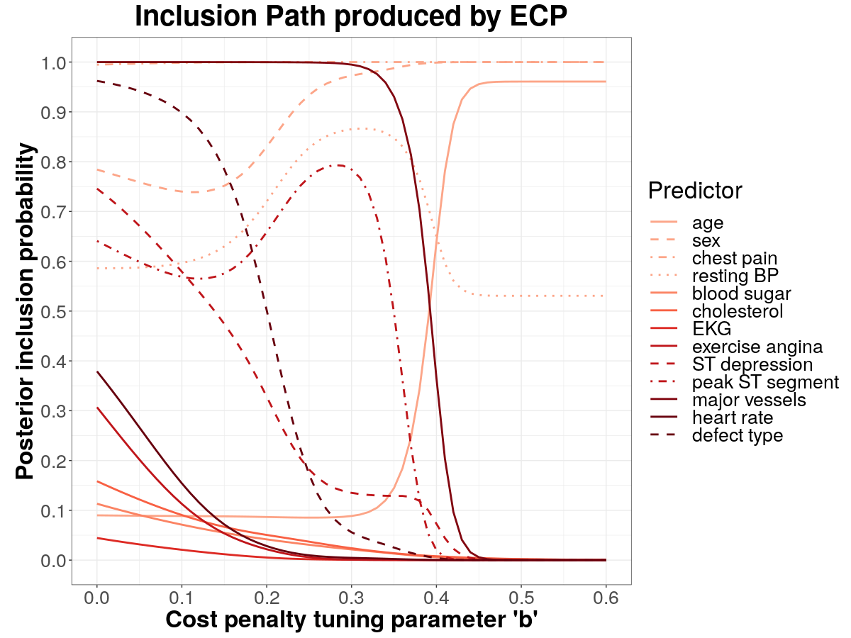
(a)

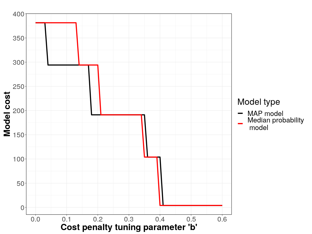
(b)

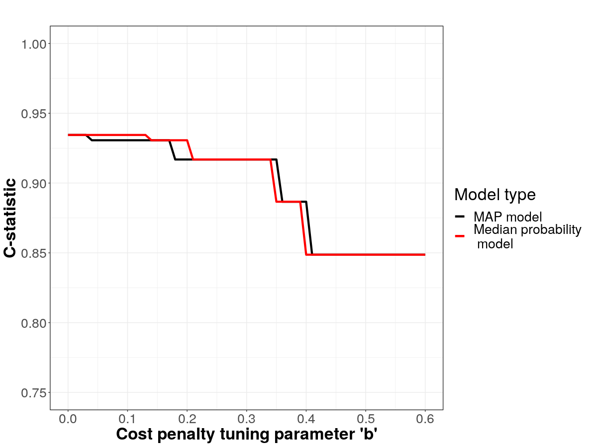
(c)

Figure 6: (a) Inclusion paths for each of the $13$ predictors from the heart disease data, (b) the cost of the MAP and median probability models, and (c) the C-statistic of the MAP and median probability models. Model selection was performed using the ECP and tuning parameter values $b$ between 0 and 0.6. Values of $b$ above $0.6$ are not shown here because there is no further change in the posterior inclusion probabilities or selected models.

Since we saw from Figure 5 that the cursory, baseline predictors included at $b=1$ may not be ideal by themselves, we might think of sliding $b$ below $1$ until reaching a set of predictors that provide a cost-penalized model whose performance is adequate and whose overall cost satisfies a hospital or patient budget. Based on a $0.5$ probability threshold, a hospital might consider, in addition to the four baseline predictors that are easy to obtain, also including predictors such as major vessels, peak ST segment, defect type, and ST depression. Suppose, for example, that a particular hospital has a maximum budget of $\$200.00$ per patient for the purpose of diagnosing heart disease. The hospital could recommend its providers record the four baseline predictors for each patient, as well as the major vessels and peak ST segment predictors, for a total cost of $\$192.20$ per patient. The inclusion paths make it clear which predictors would be included/excluded from selection at each level of cost penalization, and can be used to visualize inclusion for several predictors in any medical setting with quantifiable costs over a wide range of cost penalizations.

It is important to note that costs are often subjective, and who controls or specifies the $c_{j}$’s for the model prior is of great importance. In Section 3.4, we have used the monetary costs that were provided for this particular case study data. While the costs that are known for this case study pertain to the monetary cost to hospital and insurance stakeholders, in other applications a patient could also settle on their own set of costs based on comfort, risk, convenience, etc. and apply our proposed method. Perhaps patient advocates or medical practitioners could subjectively elicit values for the $c_{j}$’s in a useful way. A primary challenge to using our method would be to have patients or other stakeholders put forth their values for the individual $c_{j}$’s to capture/quantify the relative cost of the candidate predictors to that user.

3.5 Computation

All computations for our proposed method were performed in R. We use a Laplace approximation to approximate each of the integrated likelihoods. Specifically, for each candidate model, we use optim() in R to obtain the posterior mode of the regression coefficients and the Hessian matrix evaluated at the posterior mode by maximizing over a function containing the joint distribution of the data and regression coefficients $\boldsymbol{\beta}_{\boldsymbol{\gamma}}$. Given responses Y, a matrix $X$ containing all candidate covariates, a vector of marginal costs for each candidate covariate, and a specific value for $b$, we do the following: (1) compute the set of integrated likelihoods for every candidate model using Laplace approximation, (2) form Bayes factors as in Equation (1) for each candidate model with respect to a baseline model, (3) calculate the model prior $P(\boldsymbol{\gamma})$ for each candidate model as in Equation (9), and (4) calculate the set of $2^{p}$ posterior model probabilities (benefit-only or cost-adjusted) as in Equation (2).

Computations for the case study in Section 3.4 were completed using a $2\times\text{E}5-2683\text{v}42.1$GHz (Broadwell) CPU supercomputer from Advanced Research Computing at Virginia Tech. For a single value of $b$, it takes 16 minutes and 40 seconds to enumerate all models and calculate posterior model probabilities (benefit-only or cost-adjusted) for all $2^{13}$ candidate models.

4 Discussion

We have presented an approach to adjust cost-penalizing model priors for cost-adjusted Bayesian model selection. Our approach extends the well-established FND prior (Fouskakis et al., 2009a) by giving the practitioner the ability to adjust the level of cost penalization on candidate predictors and visualize the resulting cost-adjusted posterior inclusion probabilities. We proposed functions, according to a tuning parameter $b$, of the ratios of marginal predictor costs relative to a baseline cost. The resulting ECP prior that we study provides adjusted levels of cost penalization controlled by the practitioner via the tuning parameter. The properties that our cost ratio functions adhere to ensure that our adjusted priors can easily reproduce a benefit-only analysis and allow for unit conversion without changing model selection results, making it useful for costs measured in a variety of ways. We have shown, through simulation, that adjusting the cost penalty according to our proposed functions helps to maintain the cost penalization for larger sample sizes. Our inclusion path approach, which plots the change in cost-adjusted posterior inclusion probabilities together across a range of adjusted cost penalties, provides a visual tool to learn the relative importance of predictors when accounting for their costs and to make decisions about individual predictors to meet an overall budget. Our method can be applied to any binary outcome (e.g. diagnosis) where medical practitioners need to make a decision or prediction based on predictors with quantifiable costs.

This work extends the utility of the FND prior by adjusting the penalization on costly predictors in model selection. For example, suppose that the model selected using the FND prior has a total predictor cost that exceeds the practitioner’s or hospital’s designated budget. Then our proposed inclusion path can easily be used to see which predictor(s) have probabilities that fall below the desired threshold as the practitioner slides $b$ towards higher values. Similarly, if the practitioner seeks a higher-performing model that still penalizes candidate predictor costs to some extent, they can slide $b$ down, closer to $0$, to learn which additional predictor(s) will improve model fit without causing an undue increase in the cost per observation. We applied our approach to a data set of $297$ heart disease patients and found that decreasing the cost penalization from the FND prior helps to identify predictors that can improve the diagnosis of heart disease while still appropriately penalizing the most costly predictors. The ECP provides a useful option for adjusting the magnitude of cost penalization. The matter of cost can implicitly raise ethical concerns, especially in the case of medical applications that directly impact the health and well-being of patients. Medical practitioners would be well-positioned to apply our methods, as they have the knowledge and experience to understand how collecting different predictors may impact patients’ health, comfort, and finances and can advise on setting the cost ratio tuning parameter with these considerations in mind. We envision practitioners using a range of $g(\cdot)$ and $b$ values to study different cost penalizing settings and choose a model that best suits their budget and concerns.

Avenues for future research include developing cost-penalized model selection for a sequential decision-making framework, for example, in medical diagnoses where practitioners may order additional tests depending on a patient’s initial results. Investigation may also be done to find and recommend an upper bound for $b$ given a particular data set. Our proposed method may also be adapted and applied more broadly to non-binary response data, for example to other generalized linear models. Another possible extension could include adjusting the model space and/or prior to accommodate cost structures for grouped or discounted predictors.

Together, our tuning parameter-based functions of the cost ratios and our inclusion path proposed in this manuscript give the practitioner considerable flexibility to weigh each predictor’s cost with its modeling ability, with probabilities providing a concrete measure of inclusion, especially relative to other predictors.

References

- Adams et al. (2016) Adams, S., Beling, P. A., and Cogill, R. (2016). “Feature selection for hidden Markov models and hidden semi-Markov models.” IEEE Access, 4: 1642–1657.
-
Bang et al. (2009)
Bang, H., Edwards, A. M., Bomback, A. S., Ballantyne, C. M., Brillon, D., Callahan, M. A., Teutsch, S. M., Mushlin, A. I., and Kern, L. M. (2009).
“Development and Validation of a Patient Self-assessment Score for Diabetes Risk.”
Annals of Internal Medicine, 151(11): 775–783.
PMID: 19949143.
URL https://www.acpjournals.org/doi/abs/10.7326/0003-4819-151-11-200912010-00005 -
Barbieri and Berger (2004)
Barbieri, M. M. and Berger, J. O. (2004).
“Optimal predictive model selection.”
The Annals of Statistics, 32(3): 870 – 897.
URL https://doi.org/10.1214/009053604000000238 - Bolón-Canedo et al. (2014) Bolón-Canedo, V., Porto-Díaz, I., Sánchez-Maroño, N., and Alonso-Betanzos, A. (2014). “A framework for cost-based feature selection.” Pattern Recognition, 47(7): 2481–2489.
-
Brown et al. (1999)
Brown, B., Fearn, T., and Vannucci, M. (1999).
“The choice of variables in multivariate regression: a non-conjugate Bayesian decision theory approach.”
Biometrika, 86(3): 635–648.
URL https://doi.org/10.1093/biomet/86.3.635 - Cohn et al. (1996) Cohn, D. A., Ghahramani, Z., and Jordan, M. I. (1996). “Active learning with statistical models.” Journal of artificial intelligence research, 4: 129–145.
-
Detrano et al. (1989)
Detrano, R., Janosi, A., Steinbrunn, W., Pfisterer, M., Schmid, J.-J., Sandhu, S., Guppy, K. H., Lee, S., and Froelicher, V. (1989).
“International application of a new probability algorithm for the diagnosis of coronary artery disease.”
The American Journal of Cardiology, 64(5): 304–310.
URL https://www.sciencedirect.com/science/article/pii/0002914989905249 - Elkan (2001) Elkan, C. (2001). “The foundations of cost-sensitive learning.” In International joint conference on artificial intelligence, volume 17, 973–978. Lawrence Erlbaum Associates Ltd.
- Fan et al. (1999) Fan, W., Stolfo, S. J., Zhang, J., and Chan, P. K. (1999). “AdaCost: misclassification cost-sensitive boosting.” In Icml, volume 99, 97–105.
-
Fouskakis and Draper (2008)
Fouskakis, D. and Draper, D. (2008).
“Comparing Stochastic Optimization Methods for Variable Selection in Binary Outcome Prediction, With Application to Health Policy.”
Journal of the American Statistical Association, 103(484): 1367–1381.
URL https://doi.org/10.1198/016214508000001048 -