Pseudo-reversing and its application for
multiscaling of manifold-valued data

 

Abstract. The well-known Wiener’s lemma is a valuable statement in harmonic analysis; in the Banach space of functions with absolutely convergent Fourier series, the lemma proposes a sufficient condition for the existence of a pointwise multiplicative inverse. We call the functions that admit an inverse as reversible. In this paper, we introduce a simple and efficient method for approximating the inverse of functions, which are not necessarily reversible, with elements from the space. We term this process pseudo-reversing. In addition, we define a condition number to measure the reversibility of functions and study the reversibility under pseudo-reversing. Then, we exploit pseudo-reversing to construct a multiscale pyramid transform based on a refinement operator and its pseudo-reverse for analyzing real and manifold-valued data. Finally, we present the properties of the resulting multiscale methods and numerically illustrate different aspects of pseudo-reversing, including the applications of its resulting multiscale transform to data compression and contrast enhancement of manifold-valued sequence.

 

Keywords: Wiener’s lemma; pseudo-reversing; multiscale transform; manifold-valued sequences; compressing manifold data; manifold data enhancement.

 

Mathematics subject classification: 42C40; 65G99; 43A99; 65D15.

1 Introduction

Manifolds have become ubiquitous in modeling nonlinearities throughout many fields, ranging from science to engineering. In addition, the unceasing increase of sophisticated, modern data sets has brought many challenges in the processing of manifold data, including essential tasks like principle component analysis [22], interpolation [27], integration [9], and even the adaptation of proper neural networks to manifold values, e.g., [2, 10]. Here, we focus on multiscale transforms as a critical component in many applications over manifold data, see [3, 23, 26]. In particular, we aim to construct and analyze a new multiscale transform for manifold data.

One foundational statement in the Banach algebra theory and harmonic analysis is Wiener’s Lemma, e.g., [11, Chapter 5]. The lemma deals with the invertibility and spectrum of operators. In particular, in the Banach space of periodic functions with absolutely convergent Fourier series, the lemma suggests that if a function does not vanish, then there exists a pointwise multiplicative inverse with absolutely convergent Fourier series. These functions, having an inverse in this sense, are essential for multiscale construction, and we term them reversible. Their inverse also plays a key role, so the need for reversing rises. Unfortunately, in some cases, the reversibility is poorly possible numerically or even impossible by definition. In such cases, we aspire to suggest an alternative.

In this paper, we introduce the notion of pseudo-reversing and describe it in detail. As a natural implication of the terminology, and as one may mathematically expect, the pseudo-reverse of a reversible function coincides with its unique inverse. Conversely, applying this method to a non-reversible function produces a family of functions, depending on a continuous regularization parameter, with an absolutely convergent Fourier series. Each function approximates the corresponding inverse according to the selected regularization. Then, we study the algebraic properties of the method and introduce a condition number to determine “how reversible” functions are.

Once pseudo-reversing is established, we show its application for analyzing real-valued sequences in a multiscale fashion. In the context of multiscale transforms, the importance of Wiener’s Lemma is evoked when associating a refinement operator with a sequence in $\ell_{1}(\mathbb{Z})$, that is, the space of absolutely convergent real-valued bi-infinite sequences. Specifically, given a refinement that meets the condition of reversibility, the lemma guarantees the existence of a corresponding decimation operator. Moreover, a direct result from [29] implies that the calculation of the decimation involves an infinitely supported sequence which in turn can be truncated while maintaining accuracy [23]. The two operators, refinement and decimation, define a pyramid multiscale transform and its inverse transform.

In this study, we further generalize pyramid multiscale transforms based on a broader class of refinement operators that do not admit matching decimation operators in an executable form. In particular, we use pseudo-reversing to define the pseudo-reverse of a refinement operator. Epitomai of non-reversible operators appear in the least squares refinements introduced in [7]. Nevertheless, even with reversible operators, if their reverse conditioning is poor, we show that it is preferred to establish their associated pyramid with a pseudo-reversing operator.

As one may expect, since our generalization is based on pseudo-reversing, it comes with a cost. We present the analytical properties of the transform and show that the cost emerges in the synthesis algorithm, that is, the inverse transform, and carries undesired inaccuracies. However, we show that under mild conditions, the error is tolerable.

With the new linear multiscale transforms, we show how to adapt them to Riemannian manifolds data. First, we demonstrate how the manifold-valued transform enjoys analog results to the linear case. Specifically, we observe how the magnitude of the detail coefficients in the new multiscale representation decays with the scale. Moreover, we estimate the synthesis error from pseudo-reversing analytically for the specific manifolds with a non-negative sectional curvature.

We conclude the paper with numerical illustrations of pseudo-reversing. First, we show how to use it for constructing a decimation operator for a non-reversible subdivision scheme and the resulting multiscale. Then, we move to manifold-valued data and introduce two applications of our transform: contrast enhancement and data compression. The applications are made by systematically manipulating the detail coefficients of manifold-valued sequences. Indeed, the numerical results confirm the theoretical findings. All figures and examples were generated using a Python code package that complements the paper and is available online for reproducibility.

The paper is organized as follows. Section 2 lays the notation and definitions regarding pseudo-reversing and related terms. Section 3 introduces pyramid transform in its linear settings where in Section 4 we present the multiscale transform for manifold values. Finally, in Section 5, we describe the numerical examples.

2 Pseudo-reversing and polynomials

In this section we briefly revisit Wiener’s Lemma and present its classical formulation. In the Banach space of functions with absolutely convergent Fourier series, the lemma proposes a sufficient condition for the existence of a pointwise multiplicative inverse, within the space. We term the functions enjoying an inverse in this sense as reversible. Next, we introduce the notion of pseudo-reversing as a method to circumvent the potential non-reversibility of polynomials and describe it in detail. Finally, we present a condition number to measure the reversibility of functions and study how pseudo-reversing improves the reversibility of polynomials.

We follow similar notations presented in [11, Chapter 5]. Let $\mathbb{T}=\{z\in\mathbb{C}:|z|=1\}$ be the unit circle of the complex plane, denote by $\mathcal{A}(\mathbb{T})$ the Banach space consisting of all periodic functions $f(t)=\sum_{k\in\mathbb{Z}}a_{k}e^{2\pi ikt}$ with coefficients $\boldsymbol{a}\in\ell_{1}(\mathbb{Z})$. We endow $\mathcal{A}(\mathbb{T})$ with the norm

$$\|f\|_{\mathcal{A}}=\|\boldsymbol{a}\|_{1}=\sum_{k\in\mathbb{Z}}|a_{k}|.$$

The space $\mathcal{A}(\mathbb{T})$ becomes a Banach algebra under pointwise multiplication. In particular, $\|fg\|_{\mathcal{A}}\leq\|f\|_{\mathcal{A}}\|g\|_{\mathcal{A}}$ for any $f,g\in\mathcal{A}(\mathbb{T})$. Given a function $f\in\mathcal{A}(\mathbb{T})$, Wiener’s Lemma proposes a sufficient condition for the existence of the inverse $1/f$ in the space $\mathcal{A}(\mathbb{T})$. The classical formulation of the lemma is as follows.

Lemma 2.1.

(Wiener’s Lemma). If $f\in\mathcal{A}(\mathbb{T})$ and $f(t)\neq 0$ for all $t\in\mathbb{T}$, then also $1/f\in\mathcal{A}(\mathbb{T})$. That is, $1/f(t)=\sum_{k\in\mathbb{Z}}b_{k}e^{2\pi ikt}$ for some $\boldsymbol{b}\in\ell_{1}(\mathbb{Z})$.

Wiener’s original proof [31] uses a localization property and a partition of unit argument. An abstract proof of Lemma 2.1 is given by Gel’fand theory, see e.g. [18]. A simple and elementary proof can be found in [25].

Definition 2.1.

A function $f\in\mathcal{A}(\mathbb{T})$ is called reversible if $1/f\in\mathcal{A}(\mathbb{T})$. Moreover, $1/f$ is termed the reverse of $f$.

Lemma 2.1 guarantees that functions which do not vanish on the unit circle are reversible. One primary class of functions that is advantageous to reverse is polynomials. Indeed, in various applications, many approximating operators are uniquely characterized by polynomials, e.g., refinement operators [6]. We hence focus on the reversibility of polynomials in $\mathcal{A}(\mathbb{T})$.

Let $p(z)=a_{n}z^{n}+a_{n-1}z^{n-1}+\dots+a_{1}z+a_{0}$ be a polynomial of degree $n\in\mathbb{N}$ with complex-valued coefficients. Without loss of generality, from now on we assume that the coefficients of $p$ sum to 1, that is $p(1)=\sum_{k=0}^{n}a_{k}=1$. This requirement is compatible with (7), as we will see next in the context of refinement operators, and is frequent in approximation theory, e.g., in interpolation techniques and partition of unity, see [1] for instance. Denote by $\Lambda$ the set of all zeros of $p$ including multiplicities. That is, if $r$ is a root with multiplicity $m\in\mathbb{N}$ then $r$ appears $m$ many times in $\Lambda$. By the complete factorization theorem, we can write

$$~{}p(z)=C(p)\prod_{r\in\Lambda}(z-r)$$

where $C(p)$ is the leading coefficient of $p$. This algebraic expression makes a flexible framework to manipulate the zeros of $p$. The following definition introduces the pseudo-reverse of $p$.

Definition 2.2.

For some $\xi>0$, the pseudo-reverse of a polynomial $p$ is defined as

$$~{}p_{\xi}^{\dagger}(z)=\bigg{(}C(p_{\xi}^{\dagger})\prod_{r\in\Lambda\setminus\mathbb{T}}(z-r)\prod_{r\in\Lambda\cap\mathbb{T}}(z-(1+\xi)r)\bigg{)}^{-1}$$ (1)

where $C(p_{\xi}^{\dagger})$ is a constant depending on $\xi$ determined by $p_{\xi}^{\dagger}(1)=1$.

Note that the pseudo-reverse $p_{\xi}^{\dagger}$ of a polynomial $p$ is uniquely determined by the constant $\xi$, and is not a polynomial unless $p(z)\equiv 1$. Moreover, one can easily see that if a polynomial $p$ does not vanish on the unit circle $\mathbb{T}$, then its pseudo-reverse coincides with its reverse. That is, $p_{\xi}^{\dagger}=1/p$ for any $\xi$. The requirement that $p_{\xi}^{\dagger}(1)=1$ is proposed to ensure the equality $p_{\xi}^{\dagger}(z)p(z)=1$ at least for $z=1$. We denote the inverted term on the right hand side of (1), that is the term within the parenthesis by $p_{\xi}^{-\dagger}$. Geometrically speaking, $p_{\xi}^{-\dagger}$ approximates $p$ by displacing its zeros $\Lambda\cap\mathbb{T}$ along the rays connecting the origin with the zeros, outwards, with a displacement parameter $\xi$. Hence, by Wiener’s Lemma 2.1 the polynomial $p_{\xi}^{-\dagger}$ is reversible and $p_{\xi}^{\dagger}\in\mathcal{A}(\mathbb{T})$.

The perturbations between the polynomial coefficients of $p$ and $p_{\xi}^{-\dagger}$ can be expressed in a closed form with respect to $\xi$, but the analytical evaluations are not essential to our work. However, it is worth mentioning that the perturbations are monotonic with respect to the power of the argument $z$. In particular, the perturbation between the coefficient of $z^{j}$ in $p$ and the coefficient of $z^{j}$ in $p_{\xi}^{-\dagger}$ increases when $j$ decreases. Figure 1 illustrates the computations behind pseudo-reversing (1).

Figure 1: The computations behind pseudo-reversing polynomials (1). To pseudo-reverse a polynomial $p(z)$, we first approximate it with $p_{\xi}^{-\dagger}(z)$ by pushing its zeros with modulus 1, away from the unit circle, and then reversing to get $p_{\xi}^{\dagger}(z)$.

We proceed with two examples.

Example 2.1.

Consider the polynomial $p(z)=(z^{2}+1)/2$ which vanishes for $z=\pm i\in\mathbb{T}$. The pseudo reverse $p^{\dagger}_{\xi}$ of $p$ calculated via (1) is then

$$p_{\xi}^{\dagger}(z)=\frac{2+2\xi+\xi^{2}}{z^{2}+(1+\xi)^{2}},\quad\xi>0.$$

Example 2.2.

Consider the polynomial $p(z)=(z^{2}+z+1)/3$ which vanishes for $z=-1/2\pm i\sqrt{3}/2\in\mathbb{T}$. The pseudo reverse $p_{\xi}^{\dagger}$ of $p$ calculated via (1) is then

$$p_{\xi}^{\dagger}(z)=\frac{3+3\xi+\xi^{2}}{z^{2}+z(1+\xi)+(1+\xi)^{2}},\quad\xi>0.$$

We now present some properties of pseudo-reversing through a series of useful propositions.

Proposition 2.2.

If the polynomial $p$ has real coefficients, then so does the polynomial $p_{\xi}^{-\dagger}$.

Proof.

The assumption implies that if $r\in\Lambda$ is a zero of $p$, then so is the conjugate $\bar{r}\in\Lambda$. Moreover, the nature of pseudo-reversing (1) preserves the conjugacy property of the zeros of $p_{\xi}^{-\dagger}$. ∎

Proposition 2.3.

For any polynomial $p$, the product $p_{\xi}^{\dagger}p$ converges in norm to $1$ as $\xi$ approaches $0^{+}$. Namely,

$$\lim_{\xi\rightarrow 0^{+}}\|p_{\xi}^{\dagger}p-1\|_{\mathcal{A}}=0.$$

Proof.

Note that the polynomial coefficients of the difference $p-p_{\xi}^{-\dagger}$ are continuous with respect to the parameter $\xi$ in the positive vicinity of $0$. The uniqueness of Fourier series implies that the Fourier coefficients of $p-p_{\xi}^{-\dagger}$ vanish as $\xi\rightarrow 0^{+}$. Therefore, for any $\varepsilon>0$ there exists $\delta(\varepsilon)$ such that $\|p-p_{\xi}^{-\dagger}\|_{\mathcal{A}}<\varepsilon/\|p_{\xi}^{\dagger}\|_{\mathcal{A}}$ for $0<\xi<\delta(\varepsilon)$. Now, since $\mathcal{A}(\mathbb{T})$ is a Banach algebra, we overall get

$$\|p_{\xi}^{\dagger}p-1\|_{\mathcal{A}} =\|p_{\xi}^{\dagger}p-p_{\xi}^{\dagger}p^{-\dagger}_{\xi}\|_{\mathcal{A}}=\|p_{\xi}^{\dagger}(p-p_{\xi}^{-\dagger})\|_{\mathcal{A}}\leq\|p^{\dagger}_{\xi}\|_{\mathcal{A}}\|p-p^{-\dagger}_{\xi}\|_{\mathcal{A}}<\varepsilon$$

as required. ∎

Proposition 2.4.

If all zeros of the polynomial $p$ are on the unit circle, then $p_{\xi}^{\dagger}(z)$ converges uniformly to $1$ as $\xi$ approaches $\infty$ on every compact subset of $\mathbb{C}$.

Proof.

The assumption implies that $\Lambda\subset\mathbb{T}$. Therefore, as $\xi$ approaches infinity we have

$$\lim_{\xi\rightarrow\infty}p_{\xi}^{\dagger}(z)=\lim_{\xi\rightarrow\infty}\frac{\prod_{r\in\Lambda}(1-(1+\xi)r)}{\prod_{r\in\Lambda}(z-(1+\xi)r)}=\lim_{\xi\rightarrow\infty}\prod_{r\in\Lambda}\frac{1-r-\xi r}{z-r-\xi r}=1$$

for all $z$ in any compact subset of $\mathbb{C}$. ∎

The notion of pseudo-reversing induces the necessity of proposing a condition number to quantify the reversibility of functions in $\mathcal{A}(\mathbb{T})$. Conventionally, the condition number of a non-reversible function should take the value $\infty$, whereas the “best” reversible function should take the value $1$. Inspired by the results of [29], the next definition introduces such a condition.

Definition 2.3.

The reversibility condition $\kappa:\mathcal{A}(\mathbb{T})\rightarrow[1,\infty]$ acting on a function $f\in\mathcal{A}(\mathbb{T})$ is given by

$$~{}\kappa(f)=\frac{\sup_{z\in\mathbb{T}}|f(z)|}{\inf_{z\in\mathbb{T}}|f(z)|},$$ (2)

with the convention $\kappa(f)=\infty$ for functions with $\inf_{z\in\mathbb{T}}|f(z)|=0$.

The nature of this definition implies that $\kappa(f)$ is well defined for any $f\in\mathcal{A}(\mathbb{T})$ and returns values in $[1,\infty]$. Moreover, the condition number $\kappa(f)$ is invariant under operations that preserve the ratio between the $\sup$ and $\inf$ of $f$ over unit circle $\mathbb{T}$, e.g., under rotations, $\kappa(e^{i\theta}f)=\kappa(f)$ for any $\theta\in[0,2\pi)$. Furthermore, $\kappa$ is submultiplicative; for any two functions $f$ and $g$ we have $\kappa(fg)\leq\kappa(f)\kappa(g)$. Meaning that, reversing a product of functions would not be worse than reversing each factor solely.

The reversibility condition $\kappa(f)$ in (2) of a function $f$ is proportional to $\|1/f\|_{\mathcal{A}}$. In particular, better reversibility implies faster convergence in Fourier coefficients of the inverse. Indeed, the consistency between $\kappa(f)$ and $\|1/f\|_{\mathcal{A}}$ for any function $f$ can be evidently seen in [29]. We formulate the relation by the following corollary.

Corollary 2.5.

Let $f(t)=\sum_{k\in\mathbb{Z}}a_{k}e^{2\pi ikt}\in\mathcal{A}(\mathbb{T})$ be a positive function on the unit circle $\mathbb{T}$. Assume that $f$ is $s$-banded, that is, $a_{k}=0$ for all $|k|>s$. Fix

$$\lambda=\bigg{(}\frac{\sqrt{\kappa(f)}-1}{\sqrt{\kappa(f)}+1}\bigg{)}^{1/s}\quad\text{and}\quad C=\frac{1}{\inf_{t\in\mathbb{T}}|f(t)|}\max\bigg{\{}1,\frac{(1+\sqrt{\kappa(f)})^{2}}{2\kappa(f)}\bigg{\}}$$

where $\kappa(f)$ is the condition number (2) of $f$. Denote by $1/f(t)=\sum_{k\in\mathbb{Z}}b_{k}e^{2\pi ikt}$. Then,

$$|b_{k}|\leq C\lambda^{|k|},\quad k\in\mathbb{Z}.$$

Moreover, the coefficients $b_{k}$ are in general not banded.

The following corollary shows that pseudo-reversing (1) improves the reversibility condition.

Corollary 2.6.

Let $p$ be a polynomial with $n\in\mathbb{N}$ zeros all on the unit circle. Then,

$$\kappa(p_{\xi}^{-\dagger})=\frac{\sup_{z\in\mathbb{T}}|\prod_{r\in\Lambda}(z-(1+\xi)r)|}{\inf_{z\in\mathbb{T}}|\prod_{r\in\Lambda}(z-(1+\xi)r)|}\leq\prod_{r\in\Lambda}\frac{\sup_{z\in\mathbb{T}}|z-(1+\xi)r|}{\inf_{z\in\mathbb{T}}|z-(1+\xi)r|}=(1+2/\xi)^{n}$$

where $\xi$ is the pseudo-reversing parameter. Hence, the more we push the zeros of $p$ away from the unit circle, the more reversible the polynomial $p_{\xi}^{-\dagger}$ becomes. Consequently, using Corollary 2.5 we can get an estimation of $\|p^{\dagger}_{\xi}\|_{\mathcal{A}}$ with respect to $\xi$. In particular, the norm $\|p^{\dagger}_{\xi}\|_{\mathcal{A}}$ is bounded by a monotonically decreasing expression depending on $\xi$.

A natural implication of Corollary 2.6 and Proposition 2.3, is that there exists a trade-off between how well we approximate $p$ with $p_{\xi}^{-\dagger}$, and how reversible $p_{\xi}^{-\dagger}$ becomes. The question of finding the optimal parameter $\xi$, which simultaneously minimizes the perturbation $p-p_{\xi}^{-\dagger}$ and $\kappa(p_{\xi}^{-\dagger})$, can be answered by numerical tests, as we will see in Section 5. We conclude the section by remarking that pseudo-reversing can be applied to analytic functions. And, in the following sections we will see a use to pseudo-reversing in the context of multiscaling.

Remark 2.1.

Let $f\in\mathcal{A}(\mathbb{T})$ be an analytic function on the unit circle. We describe how to pseudo-reverse $f$ with some arbitrary error. First, we represent $f$ by its Laurent series, which converges uniformly to $f$ in some compact annulus containing the unit circle. Thanks to the analyticity of $f$, its zeros are guaranteed to be isolated. Then, we truncate the power series to get a polynomial approximating $f$ to any desirable degree. Finally, the polynomial can be reversed via (1). The result can be considered as the pseudo-reverse of $f$.

3 Linear pyramid transform based on pseudo-reversing

In this section we present the quintessential ideas and notations needed to realize our novel pyramid transform. Then, we use the notion of pseudo-reversing from Section 2 to introduce the new pyramid transform. Finally, we study its analytical properties.

3.1 Background

Multiscale transforms decompose a real-valued sequence $\boldsymbol{c}^{(J)}=\{c^{(J)}_{k}\in\mathbb{R}\;\big{|}\;k\in 2^{-J}\mathbb{Z}\}$ given over the dyadic grid of scale $J\in\mathbb{N}$, to a pyramid of the form $\{\boldsymbol{c}^{(0)};\boldsymbol{d}^{(1)},\dots,\boldsymbol{d}^{(J)}\}$ where $\boldsymbol{c}^{(0)}$ is a coarse approximation of $\boldsymbol{c}^{(J)}$ given on the integers $\mathbb{Z}$, and $\boldsymbol{d}^{(\ell)}$, $\ell=1,\dots,J$ are the detail coefficients associated with the dyadic grids $2^{-\ell}\mathbb{Z}$, respectively. We focus on transforms that involve refinement operators $\mathcal{S}$ as upsampling operators, and decimation operators $\mathcal{D}$ as their downsampling counterparts. Namely, the multiscale analysis is defined recursively by

$$~{}\boldsymbol{c}^{(\ell-1)}=\mathcal{D}\boldsymbol{c}^{(\ell)},\quad\boldsymbol{d}^{(\ell)}=\boldsymbol{c}^{(\ell)}-\mathcal{S}\boldsymbol{c}^{(\ell-1)},\quad\ell=1,\dots,J,$$ (3)

while the inverse transform, i.e., the multiscale synthesis is given by

$$~{}\boldsymbol{c}^{(\ell)}=\mathcal{S}\boldsymbol{c}^{(\ell-1)}+\boldsymbol{d}^{(\ell)},\quad\ell=1,\dots,J.$$ (4)

Practically, the role of the detail coefficients $\boldsymbol{d}^{(\ell)}$, $1\leq\ell\leq J$ in (3) is to store the data needed to reconstruct $\boldsymbol{c}^{(\ell)}$, that is, approximant of $\boldsymbol{c}^{(J)}$ at scale $\ell$, using the coarser approximant $\boldsymbol{c}^{(\ell-1)}$ of the predecessor scale $\ell-1$. Figure 2 illustrates the iterative calculations of the multiscale transform (3) and its inverse (4).

(a)

(b)

Figure 2: The pyramid transform. On the left, the analysis (3). On the right, the synthesis (4).

Let $\mathcal{S}_{\boldsymbol{\alpha}}$ be a linear, binary refinement rule of a univariate subdivision scheme $\mathcal{S}$, associated with a finitely supported mask $\boldsymbol{\alpha}$, and defined by

$$~{}\mathcal{S}_{\boldsymbol{\alpha}}(\boldsymbol{c})_{j}=\sum_{k\in\mathbb{Z}}\alpha_{j-2k}c_{k},\quad j\in\mathbb{Z}.$$ (5)

Applying the refinement $\mathcal{S}_{\boldsymbol{\alpha}}$ on a sequence $\boldsymbol{c}$ associated with the integers, yields a sequence $\mathcal{S}_{\boldsymbol{\alpha}}(\boldsymbol{c})$ associated with the values over the refined grid $2^{-1}\mathbb{Z}$. Depending on the parity of the index $k$, the refinement rule (5) can be split into two rules. Namely,

$$~{}\mathcal{S}_{\boldsymbol{\alpha}}(\boldsymbol{c})_{2j}=\sum_{k\in\mathbb{Z}}\alpha_{2k}c_{j-k}\quad\text{and}\quad\mathcal{S}_{\boldsymbol{\alpha}}(\boldsymbol{c})_{2j+1}=\sum_{k\in\mathbb{Z}}\alpha_{2k+1}c_{j-k},\quad j\in\mathbb{Z}.$$ (6)

The refinement rule (5) is termed interpolating if $\mathcal{S}_{\boldsymbol{\alpha}}(\boldsymbol{c})_{2j}=c_{j}$ for all $j\in\mathbb{Z}$. Moreover, a necessary condition for the convergence of a subdivision scheme with the refinement rule, see e.g. [6], is

$$~{}\sum_{k\in\mathbb{Z}}\alpha_{2k}=\sum_{k\in\mathbb{Z}}\alpha_{2k+1}=1$$ (7)

which is termed shift invariance. Indeed, refining a shifted data points with a shift invariant refinement gives precisely the shifted original refined outcome. With the shift invariance property (7), the rules (6) can be interpreted as moving center of masses of the elements of $\boldsymbol{c}$. We assume that any refinement mentioned is of convergent refinement operators.

Given a refinement rule $\mathcal{S}_{\boldsymbol{\alpha}}$, we look for a decimation operator $\mathcal{D}$ such that the detail coefficients $\boldsymbol{d}^{(\ell)}$ generated by the multiscale transform (3), vanish at all even indices. That is, $d^{(\ell)}_{2j}=0$ for all $j\in\mathbb{Z}$ and $\ell=1,\dots,J$. This property is beneficial for many tasks including data compression as we will see in later sections. If such a decimation operator $\mathcal{D}$ exists and involves a sequence in $\ell_{1}(\mathbb{Z})$, then $\mathcal{S}_{\boldsymbol{\alpha}}$ is termed reversible, and $\mathcal{D}$ is its reverse. This terminology will agree with Definition 2.1 as we will see next. Though, we note here that in [23, 24], such refinement is termed even-reversible.

It turns out that the operator $\mathcal{S}_{\boldsymbol{\alpha}}$ is reversible if and only if its corresponding reverse $\mathcal{D}$ is associated with a real-valued sequence $\boldsymbol{\gamma}\in\ell_{1}(\mathbb{Z})$ and takes the form

$$~{}\mathcal{D}_{\boldsymbol{\gamma}}(\boldsymbol{c})_{j}=\sum_{k\in\mathbb{Z}}\gamma_{j-k}c_{2k},\quad j\in\mathbb{Z},$$ (8)

for any real-valued sequence $\boldsymbol{c}$, while $\boldsymbol{\gamma}$ solves the convolutional equation

$$~{}(\boldsymbol{\alpha}\downarrow 2)*\boldsymbol{\gamma}=\boldsymbol{\delta},$$ (9)

where $\boldsymbol{\alpha}\downarrow 2$ denotes the even elements of $\boldsymbol{\alpha}$, i.e., $(\boldsymbol{\alpha}\downarrow 2)_{j}=\alpha_{2j}$ for $j\in\mathbb{Z}$, and $\boldsymbol{\delta}$ is the Kronecker delta sequence ($\delta_{0}=1$ and $\delta_{j}=0$ for $j\neq 0$).

Contrary to the refinement rule (5), applying the decimation operator (8) on a sequence $\boldsymbol{c}$ associated with the dyadic grid $2^{-1}\mathbb{Z}$ produces a sequence $\mathcal{D}_{\boldsymbol{\gamma}}(\boldsymbol{c})$ associated with the integers $\mathbb{Z}$, and hence the term decimation. Put simply, the decimation operator convolves the sequence $\boldsymbol{\gamma}$ with the even elements of $\boldsymbol{c}$. If a solution $\boldsymbol{\gamma}$ to (9) exists, then we call the coefficients of $\boldsymbol{\gamma}$ the decimation coefficients. Moreover, if the refinement is interpolating, that is $\boldsymbol{\alpha}\downarrow 2=\boldsymbol{\delta}$, then $\mathcal{D}_{\boldsymbol{\delta}}$ becomes the simple downsampling operator $\downarrow 2$, returning only the even elements of the input sequence. The following remark is essential to solving (9) and makes the key connection to pseudo-reversing (1) introduced in Section 2.

Remark 3.1.

We treat the entries of the sequences appearing in (9) as the Fourier coefficients of functions in $\mathcal{A}(\mathbb{T})$, and rely on the convolution theorem to solve the equation. In particular, we transfer both sides with the transform $\boldsymbol{c}\rightarrow\boldsymbol{c}(z)=\sum_{k\in\mathbb{Z}}c_{k}z^{k}$ to get

$$~{}\boldsymbol{\alpha}(z)\boldsymbol{\gamma}(z)=1.$$ (10)

Here we omitted the notation $\downarrow 2$ from $(\boldsymbol{\alpha}\downarrow 2)(z)$ for convenience. The function $\boldsymbol{c}(z)$ is termed the symbol of $\boldsymbol{c}$. In other words, given a compactly supported refinement mask $\boldsymbol{\alpha}$ defining the symbol $\boldsymbol{\alpha}(z)\in\mathcal{A}(\mathbb{T})$, we look for its reverse $\boldsymbol{\gamma}(z)$, as defined in Definition 2.1. The solution $\boldsymbol{\gamma}$ of (9) is then the absolutely convergent Fourier coefficients of $\boldsymbol{\gamma}(z)$. If $\boldsymbol{\alpha}(z)$ is not reversible, then we turn to pseudo-reversing (1) with some parameter $\xi$ – making a practical use of the notion.

Using Corollary 2.5, the solution $\boldsymbol{\gamma}$ of (9) does not have a compact support. This elevates computational challenges. However, recent study [23] has approximated the decimation operator (8) with operators involving compactly supported coefficients via proper truncation. The study was concluded with decimation operators that are concretely executable, with negligible errors.

Only when the solution $\boldsymbol{\gamma}$ of (10) is obtained, we are able to employ the refinement operator $\mathcal{S}_{\boldsymbol{\alpha}}$ of (5) together with its reverse $\mathcal{D}_{\boldsymbol{\gamma}}$ of (8) into the multiscale transform (3) as we will see next. By the nature of this construction, we will indeed have $d^{(\ell)}_{2j}=0$ for all $j\in\mathbb{Z}$ and $\ell=1,\dots,J$. Inspired by the necessity of using sequences $\boldsymbol{\alpha}$ and $\boldsymbol{\gamma}$ that do not particularly satisfy (9), we define the linear operator $\pi^{\boldsymbol{\alpha}}_{\boldsymbol{\gamma}}:\ell_{\infty}(\mathbb{Z})\rightarrow\ell_{\infty}(\mathbb{Z})$, mapping real-valued bounded sequences as follows

$$~{}\pi^{\boldsymbol{\alpha}}_{\boldsymbol{\gamma}}(\boldsymbol{c})=[(\mathcal{I}-\mathcal{S}_{\boldsymbol{\alpha}}\mathcal{D}_{\boldsymbol{\gamma}})\boldsymbol{c}]\downarrow 2,$$ (11)

where $\mathcal{I}$ is the identity operator. The operator $\pi^{\boldsymbol{\alpha}}_{\boldsymbol{\gamma}}$ measures the significance of the detail coefficients on the even indices, with one iteration of decomposition (3) when applied to a sequence $\boldsymbol{c}$. Moreover, if $\boldsymbol{\alpha}$ and $\boldsymbol{\gamma}$ satisfy (10), then $\pi^{\boldsymbol{\alpha}}_{\boldsymbol{\gamma}}$ becomes the trivial zero operator.

3.2 Linear multiscaling

Here we introduce a novel family of multiscale transforms similar to (3). What distinguishes our transforms from the ones studied in [23, 24] is that they are based on non-reversible refinement operators. One interesting family of non-reversible refinement operators is the least squares introduced in [7]. This branch of schemes was derived by fitting local least squares polynomials. We first exploit the idea of pseudo-reversing (1) to define the pseudo-reverse of a refinement operator.

Definition 3.1.

Let $\mathcal{S}_{\boldsymbol{\alpha}}$ be a refinement operator as in (5). For $\xi>0$, the decimation operator $\mathcal{D}_{\boldsymbol{\gamma}}$ of (8) is the pseudo-reverse of $\mathcal{S}_{\boldsymbol{\alpha}}$ if

$$\boldsymbol{\gamma}(z)=\boldsymbol{\alpha}^{\dagger}_{\xi}(z)$$

where $\boldsymbol{\alpha}(z)$ and $\boldsymbol{\gamma}(z)$ are defined as in Remark 3.1. i.e., if $\boldsymbol{\gamma}$ is the pseudo-reverse of $\boldsymbol{\alpha}$.

In this definition, $\boldsymbol{\gamma}$ depends on the parameter $\xi$ but we omit the latter for convenience. Moreover, we encode the Fourier coefficients of $\boldsymbol{\alpha}^{-\dagger}_{\xi}(z)$ as the even coefficients of the approximating refinement $\widetilde{\boldsymbol{\alpha}}$, while the odd values of $\widetilde{\boldsymbol{\alpha}}$ agree with the odd values of $\boldsymbol{\alpha}$. Similar to pseudo-reversing functions in $\mathcal{A}(\mathbb{T})$, the pseudo-reverse of a reversible refinement coincides with its reverse. Figure 3 illustrates the notion of pseudo-reversing refinements, and it is an analogue to Figure 1 with operators replacing functions.

Figure 3: Illustration of pseudo-reversing refinement operators.

Proposition 3.1.

If $\mathcal{S}_{\boldsymbol{\alpha}}$ is shift invariant and convergent, then so is $\mathcal{S}_{\widetilde{\boldsymbol{\alpha}}}$ for small values of $\xi$.

Proof.

The odd coefficients of the mask $\widetilde{\boldsymbol{\alpha}}$ are similar to the odd coefficients of $\boldsymbol{\alpha}$, while the even coefficients of $\widetilde{\boldsymbol{\alpha}}$ sum to $1$ due to the constant $C(\boldsymbol{\alpha}^{\dagger})$ appearing in (1). This implies the shift invariance (7) of $\mathcal{S}_{\widetilde{\boldsymbol{\alpha}}}$. As for convergence, we refer to [6] for the analysis and present here a proof sketch. Since $\mathcal{S}_{\boldsymbol{\alpha}}$ is convergent, then the refinement rule $\mathcal{S}_{\boldsymbol{\beta}}$, where the mask $\boldsymbol{\beta}$ is determined by $\boldsymbol{\alpha}(z)=(1+z)\boldsymbol{\beta}(z)$, is contractive. The contractivity of the refinement operator $\mathcal{S}_{\widetilde{\boldsymbol{\beta}}}$ corresponding to $\mathcal{S}_{\widetilde{\boldsymbol{\alpha}}}$, where $\widetilde{\boldsymbol{\alpha}}(z)=(1+z)\widetilde{\boldsymbol{\beta}}(z)$, is then naturally inherited by the continuity of $\widetilde{\boldsymbol{\alpha}}(z)$ around $\xi=0^{+}$, see Proposition 2.3. ∎

We are now in position to introduce our new multiscale transforms based on non-reversible refinement operators.

Definition 3.2.

Let $\boldsymbol{c}^{(J)}$ be a real-valued sequence of scale $J\in\mathbb{N}$, associated on the dyadic grid $2^{-J}\mathbb{Z}$, and let $\mathcal{S}_{\boldsymbol{\alpha}}$ be a refinement rule (5). The multiscale transform based on $\mathcal{S}_{\boldsymbol{\alpha}}$ is defined by

$$~{}\boldsymbol{c}^{(\ell-1)}=\mathcal{D}_{\boldsymbol{\gamma}}\boldsymbol{c}^{(\ell)},\quad\boldsymbol{d}^{(\ell)}=\boldsymbol{c}^{(\ell)}-\mathcal{S}_{\boldsymbol{\alpha}}\boldsymbol{c}^{(\ell-1)},\quad\ell=1,\dots,J,$$ (12)

where $\mathcal{D}_{\boldsymbol{\gamma}}$ is the pseudo-reverse of $\mathcal{S}_{\boldsymbol{\alpha}}$ for some $\xi>0$. The inverse transform of (12) is defined by iterating (4) for $\ell=1\dots,J$.

The major difference between the multiscale transforms (3) and (12) is that the latter based on pseudo-reversing. Therefore, it enables the employment of non-reversible refinements as upsampling operators. Next, we analyze the analytical properties of the pyramid transform (12).

3.3 Analytical properties

In multiscale analysis, and in time-frequency analysis in general, one usually wants to have a stable and perfect reconstruction. This is useful for many numerical tasks, since, we typically manipulate the detail coefficients and then reconstruct using the inverse transform. Perfect reconstruction and stability guarantee the validity of such algorithms.

In the context of our multiscale transform (12) and its inverse, perfect reconstruction means the ability to set half of the detail coefficients of each layer to zero, without losing any information after the synthesis. This property is beneficial for data compression since we can avoid storing half of the information. Therefore, half of the detail coefficients of each layer has to exhibit statistical redundancy.

The cost of using $\mathcal{S}_{\boldsymbol{\alpha}}$ with its pseudo-reverse $\mathcal{D}_{\boldsymbol{\gamma}}$ in (12) arises as a violation in the property of having zero detail coefficients on the even indices. Namely, $\pi^{\boldsymbol{\alpha}}_{\boldsymbol{\gamma}}$ of (11) is not the zero operator. Consequently, requiring small detail coefficients on the even indices raises the necessity to study the operator norm $\|\pi^{\boldsymbol{\alpha}}_{\boldsymbol{\gamma}}\|_{\infty}$, where $\boldsymbol{\alpha}$ and $\boldsymbol{\gamma}$ do not satisfy (10). The following lemma provides a global upper bound on the detail coefficients on the even indices.

Lemma 3.2.

Let $\boldsymbol{c}^{(J)}$ be a real-valued sequence, and let $\mathcal{S}_{\boldsymbol{\alpha}}$ be a refinement operator (5). Denote by $\{\boldsymbol{c}^{(0)};\boldsymbol{d}^{(1)},\dots,\boldsymbol{d}^{(J)}\}$ the multiscale representation (12) of the sequence. Then,

$$|d^{(\ell)}_{2j}|\leq\|\boldsymbol{\alpha}-\widetilde{\boldsymbol{\alpha}}\|_{\infty}\|\boldsymbol{\gamma}\|_{1},$$ (13)

for all $j\in\mathbb{Z}$ and $\ell=1,\dots,J$, where $\widetilde{\boldsymbol{\alpha}}$ is the approximating mask, and $\|\boldsymbol{\psi}\|_{\infty}=\sup_{j\in\mathbb{Z}}|\psi_{j}|$.

Proof.

Since $\boldsymbol{d}^{(\ell)}\downarrow 2$ is calculated by $\pi^{\boldsymbol{\alpha}}_{\boldsymbol{\gamma}}(\boldsymbol{c}^{(\ell)})$ for $\ell=1,\dots,J$, it is sufficient to bound the operator norm $\|\pi^{\boldsymbol{\alpha}}_{\boldsymbol{\gamma}}\|_{\infty}$. For any real-valued bounded sequence $\boldsymbol{c}$, observe that

$$\pi^{\boldsymbol{\alpha}}_{\boldsymbol{\gamma}}(\boldsymbol{c}) =[(\mathcal{I}-\mathcal{S}_{\boldsymbol{\alpha}}\mathcal{D}_{\boldsymbol{\gamma}})\boldsymbol{c}]\downarrow 2$$

$$=[(\mathcal{I}-\mathcal{S}_{\widetilde{\boldsymbol{\alpha}}}\mathcal{D}_{\boldsymbol{\gamma}}+\mathcal{S}_{\widetilde{\boldsymbol{\alpha}}}\mathcal{D}_{\boldsymbol{\gamma}}-\mathcal{S}_{\boldsymbol{\alpha}}\mathcal{D}_{\boldsymbol{\gamma}})\boldsymbol{c}]\downarrow 2$$

$$=\pi^{\widetilde{\boldsymbol{\alpha}}}_{\boldsymbol{\gamma}}(\boldsymbol{c})+[(\mathcal{S}_{\widetilde{\boldsymbol{\alpha}}}\mathcal{D}_{\boldsymbol{\gamma}}-\mathcal{S}_{\boldsymbol{\alpha}}\mathcal{D}_{\boldsymbol{\gamma}})\boldsymbol{c}]\downarrow 2$$

$$=[(\mathcal{S}_{\widetilde{\boldsymbol{\alpha}}-\boldsymbol{\alpha}}\mathcal{D}_{\boldsymbol{\gamma}})\boldsymbol{c}]\downarrow 2.$$

The last equality is obtained by the fact that $\boldsymbol{\gamma}$ is the reverse of $\widetilde{\boldsymbol{\alpha}}$, and by the linearity of the refinement (5). Now, by taking the $\ell_{\infty}$ norm we get

$$\|\pi^{\boldsymbol{\alpha}}_{\boldsymbol{\gamma}}(\boldsymbol{c})\|_{\infty}\leq\|\mathcal{S}_{\widetilde{\boldsymbol{\alpha}}-\boldsymbol{\alpha}}(\mathcal{D}_{\boldsymbol{\gamma}}\boldsymbol{c})\|_{\infty}\leq\sup_{j\in\mathbb{Z}}\sum_{k}|\widetilde{\alpha}_{j-2k}-\alpha_{j-2k}|\sum_{n}|\gamma_{k-n}|\cdot|c_{2n}|\leq\|\widetilde{\boldsymbol{\alpha}}-\boldsymbol{\alpha}\|_{\infty}\|\boldsymbol{\gamma}\|_{1}\|\boldsymbol{c}\|_{\infty}.$$

Eventually, the operator norm of $\pi^{\boldsymbol{\alpha}}_{\boldsymbol{\gamma}}$ is then

$$\|\pi^{\boldsymbol{\alpha}}_{\boldsymbol{\gamma}}\|_{\infty}=\sup_{\boldsymbol{c}\neq\boldsymbol{0}}\frac{\|\pi^{\boldsymbol{\alpha}}_{\boldsymbol{\gamma}}(\boldsymbol{c})\|_{\infty}}{\|\boldsymbol{c}\|_{\infty}}\leq\|\widetilde{\boldsymbol{\alpha}}-\boldsymbol{\alpha}\|_{\infty}\|\boldsymbol{\gamma}\|_{1},$$

as required. ∎

Lemma (3.2) offers the universal upper bound $\|\widetilde{\boldsymbol{\alpha}}-\boldsymbol{\alpha}\|_{\infty}\|\boldsymbol{\gamma}\|_{1}$ for the even detail coefficients of (12). Indeed, there is a trade-off between the quantities $\|\widetilde{\boldsymbol{\alpha}}-\boldsymbol{\alpha}\|_{\infty}$ and $\|\boldsymbol{\gamma}\|_{1}$. In particular, if $\xi$ grows, then so does the perturbation $\|\widetilde{\boldsymbol{\alpha}}-\boldsymbol{\alpha}\|_{\infty}$, and according to Corollary 2.6 the norm $\|\boldsymbol{\gamma}\|_{1}$ gets smaller.

To provide a more precise bound on the detail coefficients on the even indices, recall that, since $\widetilde{\boldsymbol{\alpha}}$ and $\boldsymbol{\gamma}$ satisfy (10), then using the pair $(\mathcal{S}_{\widetilde{\boldsymbol{\alpha}}},\mathcal{D}_{\boldsymbol{\gamma}})$ in the multiscale transform (12) result in zero detail coefficients on the even indices. The next lemma compares the detail coefficients of transform (12) when the pairs $(\mathcal{S}_{\boldsymbol{\alpha}},\mathcal{D}_{\boldsymbol{\gamma}})$ and $(\mathcal{S}_{\widetilde{\boldsymbol{\alpha}}},\mathcal{D}_{\boldsymbol{\gamma}})$ are separately used. To this purpose, we introduce the operator $\Delta$ which acts on sequences and computes the maximal consecutive difference. Namely, $\Delta\boldsymbol{c}=\sup_{j\in\mathbb{Z}}|c_{j+1}-c_{j}|$ for any real sequence $\boldsymbol{c}$.

Lemma 3.3.

Let $\boldsymbol{c}^{(J)}$ be a real-valued sequence, and let $\mathcal{S}_{\boldsymbol{\alpha}}$ be a refinement operator (5). Denote by $\{\boldsymbol{c}^{(0)};\boldsymbol{d}^{(1)},\dots,\boldsymbol{d}^{(J)}\}$ and $\{\boldsymbol{c}^{(0)};\boldsymbol{q}^{(1)},\dots,\boldsymbol{q}^{(J)}\}$ the multiscale representations (12) of $\boldsymbol{c}^{(J)}$ using the pairs $(\mathcal{S}_{\boldsymbol{\alpha}},\mathcal{D}_{\boldsymbol{\gamma}})$ and $(\mathcal{S}_{\widetilde{\boldsymbol{\alpha}}},\mathcal{D}_{\boldsymbol{\gamma}})$, respectively. Assume that $K_{\boldsymbol{\gamma}}=2\sum_{k}|\gamma_{k}||k|<\infty$. Then,

$$~{}\|\boldsymbol{d}^{(\ell)}-\boldsymbol{q}^{(\ell)}\|_{\infty}\leq\big{(}K_{\boldsymbol{\alpha},\boldsymbol{\gamma}}+K_{\widetilde{\boldsymbol{\alpha}},\boldsymbol{\gamma}}\big{)}\Delta\boldsymbol{c}^{(\ell)}$$ (14)

for $\ell=1,\dots,J$, and the positive constants

$$~{}K_{\boldsymbol{\alpha},\boldsymbol{\gamma}}=K_{\boldsymbol{\gamma}}\|\boldsymbol{\alpha}\|_{1}+K_{\boldsymbol{\alpha}}\|\boldsymbol{\gamma}\|_{1}\quad\text{and}\quad K_{\widetilde{\boldsymbol{\alpha}},\boldsymbol{\gamma}}=K_{\boldsymbol{\gamma}}\|\widetilde{\boldsymbol{\alpha}}\|_{1}+K_{\widetilde{\boldsymbol{\alpha}}}\|\boldsymbol{\gamma}\|_{1},$$ (15)

where $K_{\boldsymbol{\alpha}}=\sum_{k}|\alpha_{k}||k|$ and $K_{\widetilde{\boldsymbol{\alpha}}}=\sum_{k}|\widetilde{\alpha}_{k}||k|$.

Proof.

We explicitly calculate a general term of $\boldsymbol{q}^{(\ell)}$. For $\ell=1,\dots,J$ and $j\in\mathbb{Z}$ we have

$$q^{(\ell)}_{j} =c^{(\ell)}_{j}-\sum_{k}\widetilde{\alpha}_{j-2k}c_{k}^{(\ell-1)}=\sum_{k}\widetilde{\alpha}_{j-2k}\big{(}c_{j}^{(\ell)}-(\mathcal{D}_{\boldsymbol{\gamma}}\boldsymbol{c}^{(\ell)})_{k}\big{)}$$

$$=\sum_{k}\widetilde{\alpha}_{j-2k}\big{(}c_{j}^{(\ell)}-\sum_{n}\gamma_{k-n}c^{(\ell)}_{2n}\big{)}=\sum_{k}\widetilde{\alpha}_{j-2k}\sum_{n}\gamma_{k-n}(c_{j}^{(\ell)}-c^{(\ell)}_{2n}).$$

Consequently,

$$|q^{(\ell)}_{j}| \leq\sum_{k}|\widetilde{\alpha}_{j-2k}|\sum_{n}|\gamma_{k-n}|\big{|}c_{j}^{(\ell)}-c^{(\ell)}_{2n}\big{|}$$

$$\leq\sum_{k}|\widetilde{\alpha}_{j-2k}|\bigg{(}\sum_{n}|\gamma_{k-n}||2n-j|\bigg{)}\Delta\boldsymbol{c}^{(\ell)}$$

$$\leq\sum_{k}|\widetilde{\alpha}_{j-2k}|\bigg{(}\sum_{n}|\gamma_{k-n}|\big{(}|2n-2k|+|2k-j|\big{)}\bigg{)}\Delta\boldsymbol{c}^{(\ell)}$$

$$\leq\sum_{k}|\widetilde{\alpha}_{j-2k}|\bigg{(}K_{\boldsymbol{\gamma}}+|2k-j|\|\boldsymbol{\gamma}\|_{1}\big{)}\bigg{)}\Delta\boldsymbol{c}^{(\ell)}$$

$$\leq\big{(}K_{\boldsymbol{\gamma}}\|\widetilde{\boldsymbol{\alpha}}\|_{1}+K_{\widetilde{\boldsymbol{\alpha}}}\|\boldsymbol{\gamma}\|_{1}\big{)}\|\Delta\boldsymbol{c}^{(\ell)}\|_{\infty}=K_{\widetilde{\boldsymbol{\alpha}},\boldsymbol{\gamma}}\Delta\boldsymbol{c}^{(\ell)}.$$

Therefore, $\|\boldsymbol{q}^{(\ell)}\|_{\infty}\leq K_{\widetilde{\boldsymbol{\alpha}},\boldsymbol{\gamma}}\Delta\boldsymbol{c}^{(\ell)}$. Similar arguments (where $\widetilde{\boldsymbol{\alpha}}$ is replaced with $\boldsymbol{\alpha}$) give $\|\boldsymbol{d}^{(\ell)}\|_{\infty}\leq K_{\boldsymbol{\alpha},\boldsymbol{\gamma}}\Delta\boldsymbol{c}^{(\ell)}$. Note that the constants $K_{\boldsymbol{\alpha}}$ and $K_{\widetilde{\boldsymbol{\alpha}}}$ are finite since the corresponding masks share the same finite support. By combining both estimates into the triangle inequality we obtain the required. ∎

Lemma 3.3 induces the following theorem.

Theorem 3.4.

Let $\boldsymbol{c}^{(J)}$ be a real-valued sequence sampled from a differentiable function $f:\mathbb{R}\rightarrow\mathbb{R}$, with a bounded derivative, over the equispaced grid $2^{-J}\mathbb{Z}$. Let $\mathcal{S}_{\boldsymbol{\alpha}}$ be a refinement operator (5). Denote by $\{\boldsymbol{c}^{(0)};\boldsymbol{d}^{(1)},\dots,\boldsymbol{d}^{(J)}\}$ and $\{\boldsymbol{c}^{(0)};\boldsymbol{q}^{(1)},\dots,\boldsymbol{q}^{(J)}\}$ the multiscale representations (12) of $\boldsymbol{c}^{(J)}$ using the pairs $(\mathcal{S}_{\boldsymbol{\alpha}},\mathcal{D}_{\boldsymbol{\gamma}})$ and $(\mathcal{S}_{\widetilde{\boldsymbol{\alpha}}},\mathcal{D}_{\boldsymbol{\gamma}})$, respectively. Then,

$$~{}\|\boldsymbol{d}^{(\ell)}-\boldsymbol{q}^{(\ell)}\|_{\infty}\leq\|\boldsymbol{\gamma}\|_{1}^{J}\|f^{\prime}\|_{\infty}\big{(}K_{\boldsymbol{\alpha},\boldsymbol{\gamma}}+K_{\widetilde{\boldsymbol{\alpha}},\boldsymbol{\gamma}}\big{)}(2\|\boldsymbol{\gamma}\|_{1})^{-\ell}$$ (16)

for $\ell=1,\dots,J$, where $\|f^{\prime}\|_{\infty}=\sup_{x\in\mathbb{R}}|f^{\prime}(x)|$ and the constants $K_{\boldsymbol{\alpha},\boldsymbol{\gamma}}$ and $K_{\widetilde{\boldsymbol{\alpha}},\boldsymbol{\gamma}}$ of (15).

Proof.

Since $f$ is differentiable and bounded, then by the mean value theorem, for all $j\in\mathbb{Z}$ and a fixed $J\in\mathbb{N}$, there exists $x_{j}$ in the open segment connecting the parametrizations of $c^{(J)}_{j}$ and $c^{(J)}_{j+1}$, such that

$$|c^{(J)}_{j+1}-c^{(J)}_{j}|=2^{-J}|f^{\prime}(x_{j})|.$$

Taking the $\sup_{j\in\mathbb{Z}}$ over both sides gives the estimation $\Delta\boldsymbol{c}^{(J)}\leq 2^{-J}\|f^{\prime}\|_{\infty}$. Now, note that the decimation operator (8) can be written as $\mathcal{D}_{\boldsymbol{\gamma}}\boldsymbol{c}=\boldsymbol{\gamma}*(\boldsymbol{c}\downarrow 2)$ for any real-valued sequence $\boldsymbol{c}$. Moreover, since the convolution $*$ commutes with $\Delta$ we get

$$\Delta\boldsymbol{c}^{(\ell-1)}=\Delta(\boldsymbol{\gamma}*(\boldsymbol{c}^{(\ell)}\downarrow 2))\leq\|\boldsymbol{\gamma}\|_{1}\Delta(\boldsymbol{c}^{(\ell)}\downarrow 2)\leq 2\|\boldsymbol{\gamma}\|_{1}\Delta\boldsymbol{c}^{(\ell)}.$$

Iterating the latter inequality $J-\ell$ many times we get

$$\Delta\boldsymbol{c}^{(\ell)}\leq(2\|\boldsymbol{\gamma}\|_{1})^{J-\ell}\Delta\boldsymbol{c}^{(J)}\leq\|\boldsymbol{\gamma}\|_{1}^{J}(2\|\boldsymbol{\gamma}\|_{1})^{-\ell}\|f^{\prime}\|_{\infty}.$$

This estimation together with (14) yield the required. ∎

Theorem 3.4 implies that the effect of using $\mathcal{S}_{\widetilde{\boldsymbol{\alpha}}}$ instead of $\mathcal{S}_{\boldsymbol{\alpha}}$ in (12) is more pronounced when comparing the corresponding details on coarse scales. Consequently, the phenomenon of having small detail coefficients on the even indices has more room to be violated on coarse scales.

In the following theorem we analyze the reconstruction error, that is, the difference between the synthesized pyramids when using a non-reversible refinement $\mathcal{S}_{\boldsymbol{\alpha}}$ and its reversible approximant $\mathcal{S}_{\widetilde{\boldsymbol{\alpha}}}$ in parallel. Recall that a real-valued sequence $\boldsymbol{c}^{(J)}$ is perfectly synthesized via (4) after its analysis (12) when the pair $(\mathcal{S}_{\widetilde{\boldsymbol{\alpha}}},\mathcal{D}_{\boldsymbol{\gamma}})$ is used. To avoid abuse of notation we denote the synthesized sequence for the pair $(\mathcal{S}_{\boldsymbol{\alpha}},\mathcal{D}_{\boldsymbol{\gamma}})$ by $\boldsymbol{\zeta}^{(J)}$.

Theorem 3.5.

Let $\boldsymbol{c}^{(J)}$ be a real-valued sequence, and let $\mathcal{S}_{\boldsymbol{\alpha}}$ be a refinement operator (5). Denote by $\{\boldsymbol{c}^{(0)};\boldsymbol{d}^{(1)},\dots,\boldsymbol{d}^{(J)}\}$ its multiscale representation (12) using the pair $(\mathcal{S}_{\boldsymbol{\alpha}},\mathcal{D}_{\boldsymbol{\gamma}})$. Assume $\|\boldsymbol{\alpha}-\widetilde{\boldsymbol{\alpha}}\|_{\infty}\leq 1/\sigma$ where $\sigma$ is the support size of the even mask of $\boldsymbol{\alpha}$. Then, the synthesis sequence $\boldsymbol{\zeta}^{(J)}$ obeys

$$~{}\|\boldsymbol{c}^{(J)}-\boldsymbol{\zeta}^{(J)}\|_{\infty}\leq C\sum_{k=1}^{J}\|\boldsymbol{d}^{(k)}-\boldsymbol{q}^{(k)}\|_{\infty}+M\sum_{k=0}^{J}\sigma^{k}\|\boldsymbol{\alpha}-\widetilde{\boldsymbol{\alpha}}\|^{k}_{\infty}$$ (17)

for some constants $C>0$ and $M>0$, where $\boldsymbol{q}^{(k)}$, $k=1,\dots,J$ are the detail coefficients of $\boldsymbol{c}^{(J)}$ generated by (12) with the pair $(\mathcal{S}_{\widetilde{\boldsymbol{\alpha}}},\mathcal{D}_{\boldsymbol{\gamma}})$.

Proof.

The requirement $\|\boldsymbol{\alpha}-\widetilde{\boldsymbol{\alpha}}\|_{\infty}\leq 1/\sigma$ implies that the linear operator $\mathcal{S}_{\boldsymbol{\alpha}}-\mathcal{S}_{\widetilde{\boldsymbol{\alpha}}}$ which acts on sequences, is contractive. Namely, its operator norm is less than one since

$$\|\mathcal{S}_{\boldsymbol{\alpha}}-\mathcal{S}_{\widetilde{\boldsymbol{\alpha}}}\|_{\infty}=\|\mathcal{S}_{\boldsymbol{\alpha}-\widetilde{\boldsymbol{\alpha}}}\|_{\infty}=\sum_{k}|\alpha_{2k}-\widetilde{\alpha}_{2k}|\leq\sigma\|\boldsymbol{\alpha}-\widetilde{\boldsymbol{\alpha}}\|_{\infty}\leq 1.$$

Consequently, the operators $\{\mathcal{S}^{j}_{\boldsymbol{\alpha}-\widetilde{\boldsymbol{\alpha}}}\}_{j\in\mathbb{N}}$ are contractive as well, with the geometrically decreasing bound $\|\mathcal{S}^{j}_{\boldsymbol{\alpha}-\widetilde{\boldsymbol{\alpha}}}\|_{\infty}\leq\sigma^{j}\|\boldsymbol{\alpha}-\widetilde{\boldsymbol{\alpha}}\|^{j}_{\infty}$ for all $j\in\mathbb{N}$. Now, iterating (4) with the pair $(\mathcal{S}_{\widetilde{\boldsymbol{\alpha}}},\mathcal{D}_{\boldsymbol{\gamma}})$ reconstructs $\boldsymbol{c}^{(J)}$ as follows. We have

$$\boldsymbol{c}^{(J)}=\mathcal{S}_{\widetilde{\boldsymbol{\alpha}}}^{J}\boldsymbol{c}^{(0)}+\sum_{k=1}^{J}\mathcal{S}_{\widetilde{\boldsymbol{\alpha}}}^{J-k}\boldsymbol{q}^{(k)},$$

where $\mathcal{S}_{\widetilde{\boldsymbol{\alpha}}}^{0}=\mathcal{I}$ is the identity operator, and $\boldsymbol{q}^{(k)}$ are the detail coefficients obtained via (12) where $\mathcal{S}_{\widetilde{\boldsymbol{\alpha}}}$ is used with its reverse $\mathcal{D}_{\boldsymbol{\gamma}}$. Moreover, by iterating equation (4) starting from $\ell=J$, the reconstructed sequence $\boldsymbol{\zeta}^{(J)}$ can be expressed as

$$\boldsymbol{\zeta}^{(J)}=\mathcal{S}_{\boldsymbol{\alpha}}^{J}\boldsymbol{c}^{(0)}+\sum_{k=1}^{J}\mathcal{S}_{\boldsymbol{\alpha}}^{J-k}\boldsymbol{d}^{(k)}.$$

Therefore, by the linearity of the refinement operators we get

$$\|\boldsymbol{c}^{(J)}-\boldsymbol{\zeta}^{(J)}\|_{\infty} \leq\|\mathcal{S}_{\boldsymbol{\alpha}}^{J}\boldsymbol{c}^{(0)}-\mathcal{S}_{\widetilde{\boldsymbol{\alpha}}}^{J}\boldsymbol{c}^{(0)}\|_{\infty}+\sum_{k=1}^{J}\|\mathcal{S}_{\boldsymbol{\alpha}}^{J-k}\boldsymbol{d}^{(k)}-\mathcal{S}_{\widetilde{\boldsymbol{\alpha}}}^{J-k}\boldsymbol{q}^{(k)}\|_{\infty}$$

$$\leq\|\mathcal{S}_{\boldsymbol{\alpha}-\widetilde{\boldsymbol{\alpha}}}^{J}\boldsymbol{c}^{(0)}\|_{\infty}+\sum_{k=1}^{J}\|\mathcal{S}_{\boldsymbol{\alpha}}^{J-k}\boldsymbol{d}^{(k)}-\mathcal{S}_{\boldsymbol{\alpha}}^{J-k}\boldsymbol{q}^{(k)}\|_{\infty}+\|\mathcal{S}_{\boldsymbol{\alpha}}^{J-k}\boldsymbol{q}^{(k)}-\mathcal{S}_{\widetilde{\boldsymbol{\alpha}}}^{J-k}\boldsymbol{q}^{(k)}\|_{\infty}$$

$$\leq\sigma^{J}\|\boldsymbol{\alpha}-\widetilde{\boldsymbol{\alpha}}\|^{J}_{\infty}\|\boldsymbol{c}^{(0)}\|_{\infty}+\sum_{k=1}^{J}\|\mathcal{S}_{\boldsymbol{\alpha}}^{J-k}\|_{\infty}\|\boldsymbol{d}^{(k)}-\boldsymbol{q}^{(k)}\|_{\infty}+\sigma^{J-k}\|\boldsymbol{\alpha}-\widetilde{\boldsymbol{\alpha}}\|^{J-k}_{\infty}\|\boldsymbol{q}^{(k)}\|_{\infty}.$$

The uniform boundedness principle guarantees the existence of a constant $C>0$ such that $\sup_{j\in\mathbb{N}}\|\mathcal{S}_{\boldsymbol{\alpha}}^{j}\|_{\infty}\leq C$. And, by taking $M=\max\{\|\boldsymbol{c}^{(0)}\|_{\infty},\;\|\boldsymbol{q}^{(k)}\|_{\infty},\;k=1,\dots,J\}$ the uniform bound of the norms of the pyramid $\{\boldsymbol{c}^{(0)};\boldsymbol{q}^{(1)},\dots,\boldsymbol{q}^{(J)}\}$ we eventually obtain

$$\|\boldsymbol{c}^{(J)}-\boldsymbol{\zeta}^{(J)}\|_{\infty} \leq C\sum_{k=1}^{J}\|\boldsymbol{d}^{(k)}-\boldsymbol{q}^{(k)}\|_{\infty}+M\sum_{k=0}^{J}\sigma^{J-k}\|\boldsymbol{\alpha}-\widetilde{\boldsymbol{\alpha}}\|^{J-k}_{\infty},$$

as required. ∎

The assumption $\|\boldsymbol{\alpha}-\widetilde{\boldsymbol{\alpha}}\|_{\infty}\leq 1/\sigma$ appearing in Theorem 3.5 is mild because the maximal perturbation can be bounded as a direct result of Proposition 2.4. Moreover, since the upper bound in (17) grows with respect to the scale $J$, it is possible to reduce its value by considering only few iterations in multiscaling (12), rather than $J$ times. Specifically, for a fixed number of iterations $1\leq m<J$, we can decompose $\boldsymbol{c}^{(J)}$ via (12) $m$ many times into the pyramid $\{\boldsymbol{c}^{(J-m)};\boldsymbol{d}^{(J-m+1)},\dots,\boldsymbol{d}^{(J)}\}$ and get a better synthesis. In order to have a good synthesis algorithm, that is, small-enough upper bound (17), we impose a priori on the analyzed sequence $\boldsymbol{c}^{(J)}$ in Theorem 3.5. Particularly, similar to Theorem 3.4, we assume $\boldsymbol{c}^{(J)}$ to be sampled from a differentiable function as the following corollary argues.

Corollary 3.6.

Under the conditions of Theorem 3.5, assume that $\boldsymbol{c}^{(J)}$ is sampled from a differentiable function $f:\mathbb{R}\rightarrow\mathbb{R}$ with a bounded derivative, over the equispaced grid $2^{-J}\mathbb{Z}$. Then,

$$~{}\|\boldsymbol{c}^{(J)}-\boldsymbol{\zeta}^{(J)}\|_{\infty}\leq C\|\boldsymbol{\gamma}\|_{1}^{J}\|f^{\prime}\|_{\infty}\big{(}K_{\boldsymbol{\alpha},\boldsymbol{\gamma}}+K_{\widetilde{\boldsymbol{\alpha}},\boldsymbol{\gamma}}\big{)}\sum_{k=1}^{J}(2\|\boldsymbol{\gamma}\|_{1})^{-k}+M\sum_{k=0}^{J}\sigma^{k}\|\boldsymbol{\alpha}-\widetilde{\boldsymbol{\alpha}}\|^{k}_{\infty}$$ (18)

where the constants $K_{\boldsymbol{\alpha},\boldsymbol{\gamma}}$, $K_{\widetilde{\boldsymbol{\alpha}},\boldsymbol{\gamma}}$, $C$ and $M$ appear in (15) and (17). Therefore, if both quantities $\|f^{\prime}\|_{\infty}$ and $\|\boldsymbol{\alpha}-\widetilde{\boldsymbol{\alpha}}\|_{\infty}$ are small, then iterating (4) is efficient for recovering the analyzed sequence in (12).

Figure 4 epitomizes the theoretical results of this section; it illustrates the analysis and the synthesis with the pairs $(\mathcal{S}_{\boldsymbol{\alpha}},\mathcal{D}_{\boldsymbol{\gamma}})$ and $(\mathcal{S}_{\widetilde{\boldsymbol{\alpha}}},\mathcal{D}_{\boldsymbol{\gamma}})$. We conclude the section with two remarks.

Remark 3.2.

The method of pseudo-reversing (1) can be a remedy for reversible refinements $\mathcal{S}_{\boldsymbol{\alpha}}$ with bad reversibility condition. That is, refinements with high values of $\kappa(\boldsymbol{\alpha})$ in (2). Although their reverses involve decimation coefficients $\boldsymbol{\gamma}\in\ell_{1}(\mathbb{Z})$, their decay rate may be poor due to Corollary 2.6 and thus requiring a large truncation support [23] for implementation. Indeed, a better decay rate can be enforced by pushing the zeros of $\boldsymbol{\alpha}(z)$ that are outside of the unit disk, further from the boundary $\mathbb{T}$, in a similar manner to pseudo-reversing. Refinements from the family of B-spline [4] subdivision schemes could play as key examples to such operators, as shown in Section 5.

Remark 3.3.

Despite having a perfect synthesis algorithm, the reason we avert using the pair $(\mathcal{S}_{\widetilde{\boldsymbol{\alpha}}},\mathcal{D}_{\boldsymbol{\gamma}})$ in multiscale transforms is that the approximated refinement $\mathcal{S}_{\widetilde{\boldsymbol{\alpha}}}$ may not inherit the essential properties of the original $\mathcal{S}_{\boldsymbol{\alpha}}$, e.g., the capability of some refinements to produce smooth limit functions may be lost when approximating $\mathcal{S}_{\boldsymbol{\alpha}}$ with $\mathcal{S}_{\widetilde{\boldsymbol{\alpha}}}$.

Figure 4: Two pyramid transforms of the sequence $\boldsymbol{c}^{(J)}$. With a refinement operator $\mathcal{S}_{\boldsymbol{\alpha}}$, the upper transform uses the pair $(\mathcal{S}_{\boldsymbol{\alpha}},\mathcal{D}_{\boldsymbol{\gamma}})$ while the lower transform uses $(\mathcal{S}_{\widetilde{\boldsymbol{\alpha}}},\mathcal{D}_{\boldsymbol{\gamma}})$. The decimation operator $\mathcal{D}_{\boldsymbol{\gamma}}$ is mutual in both transforms and is the pseudo-reverse of $\mathcal{S}_{\boldsymbol{\alpha}}$.

4 Multiscaling manifold values

In this section we adapt the multiscale transform (12) to manifold-valued sequences. To this purpose, it is necessary to adapt the operators $\mathcal{S}_{\boldsymbol{\alpha}}$ and $\mathcal{D}_{\boldsymbol{\gamma}}$ of (5) and (8) to manifolds, as well as defining the analogues to the elementary operations ‘$-$’ and ‘$+$’ appearing in the transform and its inverse. Indeed, there are various methods for adapting the multiscale transform, but we follow the same adaptations and definitions of [23].

Let $\mathcal{M}$ be an open complete Riemannian manifold equipped with Riemannian metric $\langle\cdot,\cdot\rangle$. The Riemannian geodesic distance $\rho:\mathcal{M}^{2}\rightarrow\mathbb{R}^{+}$ is defined by

$$~{}\rho(x,y)=\inf_{\Gamma}\int_{a}^{b}|\dot{\Gamma}(t)|dt,$$ (19)

where $\Gamma:[a,b]\rightarrow\mathcal{M}$ is a curve connecting the points $x=\Gamma(a)$ and $y=\Gamma(b)$, and $|\cdot|^{2}=\langle\cdot,\cdot\rangle$.

Based on the Riemannian geodesic (19), the operators $\mathcal{S}_{\boldsymbol{\alpha}}$ and $\mathcal{D}_{\boldsymbol{\gamma}}$ of (5) and (8) are adapted to $\mathcal{M}$ respectively by the optimization problems

$$~{}\mathcal{T}_{\boldsymbol{\alpha}}(\boldsymbol{c})_{j}=\text{argmin}_{x\in\mathcal{M}}\sum_{k\in\mathbb{Z}}\alpha_{j-2k}\rho^{2}(x,c_{k}),\quad j\in\mathbb{Z},$$ (20)

and

$$~{}\mathcal{Y}_{\boldsymbol{\gamma}}(\boldsymbol{c})_{j}=\text{argmin}_{x\in\mathcal{M}}\sum_{k\in\mathbb{Z}}\gamma_{j-k}\rho^{2}(x,c_{2k}),\quad j\in\mathbb{Z},$$ (21)

for $\mathcal{M}$-valued sequences $\boldsymbol{c}$. When the solution of (20) or (21) exists uniquely, we term the solution as the Riemannian center of mass [15]. It is also termed Karcher mean for matrices and Frèchet mean in more general metric spaces, see [20].

The global well-definedness of (20) and (21) when $\boldsymbol{\alpha}$ and $\boldsymbol{\gamma}$ have non-negative entries is studied in [21]. Moreover, in the framework where $\mathcal{M}$ has a non-positive sectional curvature, if the mask $\boldsymbol{\alpha}$ is shift invariant (7), then a globally unique solution to problem (20) can be found, see e.g., [19, 16, 28]. Similar argument applies to problem (21) since the elements of $\boldsymbol{\gamma}$ must sum to 1 due to (10). Recent studies of manifolds with positive sectional curvature show necessary conditions for uniqueness on the spread of points with respect to the injectivity radius of $\mathcal{M}$ [5, 17]. We focus on $\mathcal{M}$-valued sequences $\boldsymbol{c}$ that are admissible in the sense that, both (20) and (21) are uniquely solved for any shift invariant mask $\boldsymbol{\alpha}$ and sequence $\boldsymbol{\gamma}$.

We say that the nonlinear operator $\mathcal{T}_{\boldsymbol{\alpha}}$ is non-reversible if its linear counterpart $\mathcal{S}_{\boldsymbol{\alpha}}$ is non-reversible. Similar to pseudo-reversing refinements in the linear setting, as in Definition 3.1, we define the pseudo-reverse of the manifold-valued refinement $\mathcal{T}_{\boldsymbol{\alpha}}$. Namely, we say that the decimation operator $\mathcal{Y}_{\boldsymbol{\gamma}}$ is the pseudo-reverse of $\mathcal{T}_{\boldsymbol{\alpha}}$ if for some $\xi>0$, we have $\boldsymbol{\gamma}$ is the pseudo-reverse of $\boldsymbol{\alpha}$. In short, Figure 3 illustrates the calculations behind pseudo-reversing refinement operators in the manifold setting, where the linear operators are replaced with the nonlinear ones.

Given a Riemannian manifold $\mathcal{M}$, recall that the exponential mapping $\text{exp}_{p}$ maps a vector $v$ in the tangent space $T_{p}\mathcal{M}$ to the end point of a geodesic of length $\|v\|$, which emanates from $p\in\mathcal{M}$ with initial tangent vector $v$. Inversely, $\text{log}_{p}$ is the inverse map of $\text{exp}_{p}$ that takes an $\mathcal{M}$-valued element $q$ and returns a vector in the tangent space $T_{p}\mathcal{M}$. Following similar notations used in [13] and [23], we denote both maps by

$$\text{log}_{p}(q)=q\ominus p\quad\text{and}\quad\text{exp}_{p}(v)=p\oplus v.$$ (22)

We have thus defined the analogues $\ominus$ and $\oplus$ of the ‘$-$’ and ‘$+$’ operations appearing in (12), respectively. For any point $p\in\mathcal{M}$ we use the following notation $\ominus:\mathcal{M}^{2}\rightarrow T_{p}\mathcal{M}$ and $\oplus:\mathcal{M}\times T_{p}\mathcal{M}\rightarrow\mathcal{M}$. Then, the compatibility condition is

$$(p\oplus v)\ominus p=v,$$

for all $v\in T_{p}\mathcal{M}$ within the injectivity radius of $\mathcal{M}$. With the operators (20), (21) and (22) in hand, we are able to define the analogue of Definition 3.2.

Definition 4.1.

Let $\mathcal{M}$ be a Riemannian manifold, and let $\boldsymbol{c}^{(J)}$ be an admissible $\mathcal{M}$-valued sequence of scale $J\in\mathbb{N}$ parameterized over the dyadic grid $2^{-J}\mathbb{Z}$, and let $\mathcal{T}_{\boldsymbol{\alpha}}$ be a refinement rule (20). The multiscale transform is defined by

$$~{}\boldsymbol{c}^{(\ell-1)}=\mathcal{Y}_{\boldsymbol{\gamma}}\boldsymbol{c}^{(\ell)},\quad\boldsymbol{d}^{(\ell)}=\boldsymbol{c}^{(\ell)}\ominus\mathcal{T}_{\boldsymbol{\alpha}}\boldsymbol{c}^{(\ell-1)},\quad\ell=1,\dots,J,$$ (23)

where $\mathcal{Y}_{\boldsymbol{\gamma}}$ is the pseudo-reverse of $\mathcal{T}_{\boldsymbol{\alpha}}$ for some $\xi>0$. The inverse transform of (23) is defined by iterating

$$~{}\boldsymbol{c}^{(\ell)}=\mathcal{T}_{\boldsymbol{\alpha}}\boldsymbol{c}^{(\ell-1)}\oplus\boldsymbol{d}^{(\ell)}$$ (24)

for $\ell=1\dots,J$.

A first difference between the manifold and linear versions of the transform lies in the detail coefficients. In particular, for the manifold-valued transform (23), the sequences $\boldsymbol{c}^{(\ell)}$, $\ell=1,2,\dots,J$ are $\mathcal{M}$-valued, while the detail coefficients $\boldsymbol{d}^{(\ell)}$ are elements in the tangent bundle $T\mathcal{M}=\bigcup_{p\in\mathcal{M}}\{p\}\times T_{p}\mathcal{M}$ associated with $\mathcal{M}$.

To investigate the properties of the multiscale transform (23) we use the approximated refinement operator $\mathcal{T}_{\widetilde{\boldsymbol{\alpha}}}$. Particularly, the pair $(\mathcal{T}_{\widetilde{\boldsymbol{\alpha}}},\mathcal{Y}_{\boldsymbol{\gamma}})$ produces detail coefficients that vanish in the tangent bundle $T\mathcal{M}$, at the even indices, when enrolled into (23). Namely, when $\mathcal{T}_{\boldsymbol{\alpha}}$ is replaced by $\mathcal{T}_{\widetilde{\boldsymbol{\alpha}}}$. To this purpose, we present the following $\mu$ and $\Delta_{\mathcal{M}}$ notations

$$\mu(\boldsymbol{c},\boldsymbol{m})=\sup_{j\in\mathbb{Z}}\rho(c_{j},m_{j})\quad\text{and}\quad\Delta_{\mathcal{M}}\boldsymbol{c}=\sup_{j\in\mathbb{Z}}\rho(c_{j+1},c_{j}).$$

The weak convergence result of [30], together with Proposition 3.1, guarantee that for a dense enough sequence $\boldsymbol{c}$, i.e., small value of $\Delta_{\mathcal{M}}\boldsymbol{c}$, we have that

$$~{}\mu(\mathcal{T}_{\boldsymbol{\alpha}}\boldsymbol{c},\mathcal{T}_{\widetilde{\boldsymbol{\alpha}}}\boldsymbol{c})\leq R\Delta_{\mathcal{M}}\boldsymbol{c},$$ (25)

for some constant $R>0$ depending on $\xi$ of (1). This estimation is required to show the stability of the inverse multiscale transform (24) as we will see in Theorem 4.2. The following definition is then necessary. We say that the refinement operator $\mathcal{T}_{\boldsymbol{\alpha}}$ of (20) is stable if there exists a constant $K>0$ such that

$$~{}\mu(\mathcal{T}_{\boldsymbol{\alpha}}\boldsymbol{c},\mathcal{T}_{\boldsymbol{\alpha}}\boldsymbol{m})\leq K\mu(\boldsymbol{c},\boldsymbol{m}),$$ (26)

for all admissible sequences $\boldsymbol{c}$ and $\boldsymbol{m}$. The stability condition has been studied in [12]. We are now ready to present the analogue of Lemma 3.3.

Lemma 4.1.

Let $\boldsymbol{c}^{(J)}$ be admissible $\mathcal{M}$-valued sequence, and $\mathcal{T}_{\boldsymbol{\alpha}}$ a stable refinement operator (26). Denote by $\{\boldsymbol{c}^{(0)};\boldsymbol{d}^{(1)},\dots,\boldsymbol{d}^{(J)}\}$ and $\{\boldsymbol{c}^{(0)};\boldsymbol{q}^{(1)},\dots,\boldsymbol{q}^{(J)}\}$ the multiscale transforms (23) of $\boldsymbol{c}^{(J)}$ using the pairs $(\mathcal{T}_{\boldsymbol{\alpha}},\mathcal{Y}_{\boldsymbol{\gamma}})$ and $(\mathcal{T}_{\widetilde{\boldsymbol{\alpha}}},\mathcal{Y}_{\boldsymbol{\gamma}})$, respectively. Then,

$$~{}\|\boldsymbol{d}^{(\ell)}-\boldsymbol{q}^{(\ell)}\|_{\infty}\leq Q\Delta_{\mathcal{M}}\boldsymbol{c}^{(\ell)}$$ (27)

for some constant $Q>0$.

Proof.

Note that since both pyramid representations use $\mathcal{Y}_{\boldsymbol{\gamma}}$ as their decimation operator, then both $d_{j}^{(\ell)}$ and $q_{j}^{(\ell)}$ are emanated from the same point $c^{(\ell)}_{j}\in\mathcal{M}$, and thus $d_{j}^{(\ell)}-q_{j}^{(\ell)}\in T_{c^{(\ell)}_{j}}\mathcal{M}$. Theorem 5.7 of [23] guarantees the existence of a constant $Q/2$ such that $\|\boldsymbol{d}^{(\ell)}\|_{\infty}$ and $\|\boldsymbol{q}^{(\ell)}\|_{\infty}$ are bounded by $Q/2\cdot\Delta_{\mathcal{M}}\boldsymbol{c}^{(\ell)}$. Hence, a simple triangle inequality gives the required. ∎

Lemma (4.1) shows that the magnitude of the even coefficients $d^{(\ell)}_{2j}$, $j\in\mathbb{Z}$ of (23) depend on the scale $\ell$. In particular, the coefficients are closer to $0$ when the scale $\ell$ is high, and therefore can be omitted when synthesizing $\boldsymbol{c}^{(J)}$ via (24). We next analyze the synthesis error.

It turns out that an analogue of Theorem 3.5 can be obtained intrinsically, when the curvature of the manifold is bounded. Next, we present such a result assuming $\mathcal{M}$ is complete, open manifold with non-negative sectional curvature. For that, we recall two classical theorems: the first and second Rauch comparison theorems. For more details see [14, Chapter 3] and references therein.

Let $p_{j}\in\mathcal{M}$, $j=1,2$ be two points and $v_{j}\in T_{p_{j}}\mathcal{M}$ their vectors in the tangent spaces such that $\|v_{1}\|=\|v_{2}\|$ and the value is smaller than the injectivity radius of $\mathcal{M}$. Let $G(p_{1},p_{2})$ be the geodesic line connecting $p_{1}$ and $p_{2}$ and $\operatorname{PG}_{p_{2}}(v_{1})\in T_{p_{2}}\mathcal{M}$ be the parallel transport of $v_{1}$ along $G(p_{1},p_{2})$ to $T_{p_{2}}\mathcal{M}$. Then, the first Rauch theorem suggests that

$$\rho\big{(}p_{2}\oplus v_{2},p_{2}\oplus\operatorname{PG}_{p_{2}}(v_{1})\big{)}\leq\|v_{2}-\operatorname{PG}_{p_{2}}(v_{1})\|.$$ (28)

In addition, the second Rauch theorem implies that

$$\rho\big{(}p_{1}\oplus v_{1},p_{2}\oplus\operatorname{PG}_{p_{2}}(v_{1})\big{)}\leq\rho(p_{1},p_{2}).$$ (29)

We are now ready for the stability conclusion.

Theorem 4.2.

Let $\boldsymbol{c}^{(J)}$ be admissible $\mathcal{M}$-valued sequence where $\mathcal{M}$ is a complete, open manifold with non-negative sectional curvature. Denote by $\{\boldsymbol{c}^{(0)};\boldsymbol{d}^{(1)},\dots,\boldsymbol{d}^{(J)}\}$ its multiscale transform (23) based on the refinement operator $\mathcal{T}_{\boldsymbol{\alpha}}$ and its pseudo-reverse $\mathcal{Y}_{\boldsymbol{\gamma}}$. Assume $\mathcal{T}_{\boldsymbol{\alpha}}$ is stable with a constant $K$ as in (26). Then, the synthesis sequence $\boldsymbol{\zeta}^{(J)}$ obeys

$$~{}\mu(\boldsymbol{c}^{(J)},\boldsymbol{\zeta}^{(J)})\leq L\Delta_{\mathcal{M}}\boldsymbol{\zeta}^{(J)}+\sum_{k=1}^{J}K^{J-k}\|\widehat{\boldsymbol{d}}^{(k)}-\widehat{\boldsymbol{q}}^{(k)}\|_{\infty},$$ (30)

for some constant $L>0$, where $\boldsymbol{q}^{(k)}$ are the detail coefficients of (23) generated by the pair $(\mathcal{T}_{\widetilde{\boldsymbol{\alpha}}},\mathcal{Y}_{\boldsymbol{\gamma}})$, and $\widehat{\psi}_{j}^{(k)}=\operatorname{PG}_{(\mathcal{T}_{\boldsymbol{\alpha}}\boldsymbol{\zeta}^{(k-1)})_{j}}(\psi_{j}^{(k)})$ for any sequence $\boldsymbol{\psi}\in T\mathcal{M}$.

Proof.

As stated in the theorem, we denote by $\{\boldsymbol{c}^{(0)};\boldsymbol{q}^{(1)},\dots,\boldsymbol{q}^{(J)}\}$ the multiscale transform (23) based on the pair $(\mathcal{T}_{\widetilde{\boldsymbol{\alpha}}},\mathcal{Y}_{\boldsymbol{\gamma}})$. Without loss of generality we assume that $\|{d}_{j}^{(\ell)}\|=\|q_{j}^{(\ell)}\|$ with values smaller than the injectivity radius of $\mathcal{M}$, for all $\ell=1,\ldots,J$ and $j\in\mathbb{Z}$. Indeed, we allow the details to differ only by their mutual angle and not magnitude. We may remove this obstacle by using a more technical calculation. By using the estimations (28) and (29) we get

$$\mu(\boldsymbol{c}^{(k)},\boldsymbol{\zeta}^{(k)}) =\mu(\mathcal{T}_{\boldsymbol{\alpha}}\boldsymbol{c}^{(k-1)}\oplus\boldsymbol{d}^{(k)},\mathcal{T}_{\widetilde{\boldsymbol{\alpha}}}\boldsymbol{\zeta}^{(k-1)}\oplus\boldsymbol{q}^{(k)})$$

$$\leq\mu(\mathcal{T}_{\boldsymbol{\alpha}}\boldsymbol{c}^{(k-1)}\oplus\boldsymbol{d}^{(k)},\mathcal{T}_{\boldsymbol{\alpha}}\boldsymbol{\zeta}^{(k-1)}\oplus\widehat{\boldsymbol{d}}^{(k)})$$

$$\qquad\qquad\qquad\qquad+\mu(\mathcal{T}_{\boldsymbol{\alpha}}\boldsymbol{\zeta}^{(k-1)}\oplus\widehat{\boldsymbol{d}}^{(k)},\mathcal{T}_{\boldsymbol{\alpha}}\boldsymbol{\zeta}^{(k-1)}\oplus\widehat{\boldsymbol{q}}^{(k)})$$

$$\qquad\qquad\qquad\qquad\qquad\qquad\qquad+\mu(\mathcal{T}_{\boldsymbol{\alpha}}\boldsymbol{\zeta}^{(k-1)}\oplus\widehat{\boldsymbol{q}}^{(k)},\mathcal{T}_{\widetilde{\boldsymbol{\alpha}}}\boldsymbol{\zeta}^{(k-1)}\oplus\boldsymbol{q}^{(k)})$$

$$\leq K\mu(\boldsymbol{c}^{(k-1)},\boldsymbol{\zeta}^{(k-1)})+\|\widehat{\boldsymbol{d}}^{(k)}-\widehat{\boldsymbol{q}}^{(k)}\|_{\infty}+\mu(\mathcal{T}_{\boldsymbol{\alpha}}\boldsymbol{\zeta}^{(k-1)},\mathcal{T}_{\widetilde{\boldsymbol{\alpha}}}\boldsymbol{\zeta}^{(k-1)})$$

for $1\leq k\leq J$. Now, using (25), there exists a constant $R>0$ such that

$$\mu(\mathcal{T}_{\boldsymbol{\alpha}}\boldsymbol{\zeta}^{(k-1)},\mathcal{T}_{\widetilde{\boldsymbol{\alpha}}}\boldsymbol{\zeta}^{(k-1)})\leq R\Delta_{\mathcal{M}}\boldsymbol{\zeta}^{(k-1)}.$$

Moreover, Proposition 5.4 in [23] guarantees the existence of a constant $P>1$ such that

$$\Delta_{\mathcal{M}}\boldsymbol{\zeta}^{(k-1)}\leq(2P)^{J-k+1}\Delta_{\mathcal{M}}\boldsymbol{\zeta}^{(J)}.$$

Overall we have

$$\mu(\boldsymbol{c}^{(k)},\boldsymbol{\zeta}^{(k)})\leq K\mu(\boldsymbol{c}^{(k-1)},\boldsymbol{\zeta}^{(k-1)})+\|\widehat{\boldsymbol{d}}^{(k)}-\widehat{\boldsymbol{q}}^{(k)}\|_{\infty}+R(2P)^{J-k+1}\Delta_{\mathcal{M}}\boldsymbol{\zeta}^{(J)}.$$

By iterating the latter inequality starting from $k=J$ we get

$$\mu(\boldsymbol{c}^{(J)},\boldsymbol{\zeta}^{(J)})\leq L\Delta_{\mathcal{M}}\boldsymbol{\zeta}^{(J)}+\sum_{k=1}^{J}K^{J-k}\|\widehat{\boldsymbol{d}}^{(k)}-\widehat{\boldsymbol{q}}^{(k)}\|_{\infty},$$

where $L=2PR\sum_{k=1}^{J}(2KP)^{J-k}$ as required. ∎

Note that the upper bound in (30) grows with $J$, while the quantity $\Delta_{\mathcal{M}}\boldsymbol{\zeta}^{(J)}$ is small in general because $\mathcal{T}_{\boldsymbol{\alpha}}$ is convergent. Moreover, to guarantee a good synthesis algorithm, one can reduce the number of decompositions in the multiscale transform (23). Specifically, for a fixed integer $1\leq m<J$, we decompose $\boldsymbol{c}^{(J)}$ via iterations of (23) $m$ many times to get the pyramid $\{\boldsymbol{c}^{(J-m)};\boldsymbol{d}^{(J-m+1)},\dots,\boldsymbol{d}^{(J)}\}$. The smaller $m$ is, the better the synthesis becomes.

We conclude this section by remarking that if the analyzed sequence $\boldsymbol{c}^{(J)}$ is sampled from a regular differentiable curve $\Gamma\subset\mathcal{M}$ over the arc-length parametrization grid $2^{-J}\mathbb{Z}$, then we instantly have that $\Delta_{\mathcal{M}}\boldsymbol{c}^{(J)}\leq\|\nabla\Gamma\|_{\infty}2^{-J}$ where $\|\nabla\Gamma\|_{\infty}=\sup_{j}\|\nabla\Gamma(j)\|$. Under this assumption, one can obtain more precise estimations of the bounds (27) and (30), see [23] for more elaborations.

5 Applications and numerical examples

In this section we illustrate different applications of our multiscale transforms. All results are reproducible via a package of Python code available online at https://github.com/WaelMattar/Pseudo-reversing.git. We start with numerical illustrations of pseudo-reversing subdivision schemes as refinement operators, in the linear setting, as Figure (3) shows.

5.1 Pseudo-reversing subdivision schemes

Let $\mathcal{S}_{\boldsymbol{\alpha}}$ be the subdivision scheme (5) given with the mask

$$~{}\boldsymbol{\alpha}=\bigg{[}\displaystyle\frac{1}{4},\;\frac{1}{3},\;\frac{1}{4},\;\frac{1}{3},\;\frac{1}{4},\;\frac{1}{3},\;\frac{1}{4}\bigg{]}\quad\text{supported on}\quad[-3,-2,-1,0,1,2,3].$$ (31)

This subdivision is a member of a broader family of least-squares schemes [7], and its corresponding symbol $\boldsymbol{\alpha}(z)$ of (10) is given by

$$~{}\boldsymbol{\alpha}(z)=\frac{1}{3z}+\frac{1}{3}+\frac{z}{3}.$$ (32)

The polynomial $z\boldsymbol{\alpha}(z)$ appears in Example 2.2 and it possesses two zeros on the unit circle; $-1/2\pm i\sqrt{3}/2$. Figure 5 demonstrates the effect of pseudo-reversing the symbol $\boldsymbol{\alpha}$ with different parameters of $\xi$, highlighting the resulting tradeoff; when $\xi$ values are large, we obtain better-decaying decimation coefficients but also larger deviations from the original sequence. On the contrary, when we perturb only slightly with small $\xi$ values, the decimation, comprised of the reversed sequence, grows significantly, making its practical use less feasible.

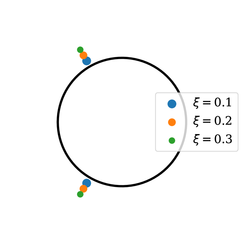
(a) Displacements of zeros relative to $\mathbb{T}$.

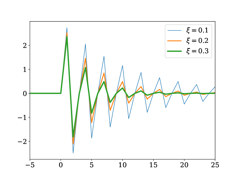
(b) Decimation coefficients.

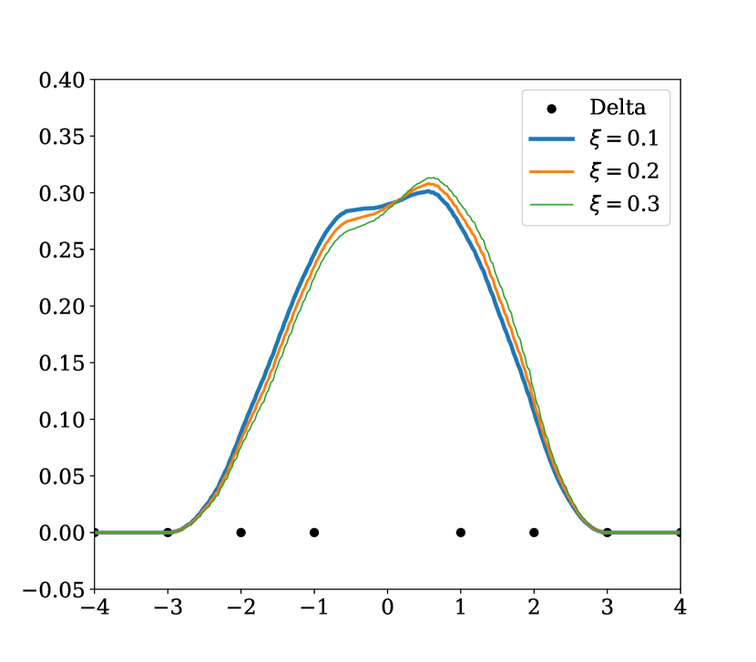
(c) Basic limit functions of $\mathcal{S}_{\widetilde{\boldsymbol{\alpha}}}$.

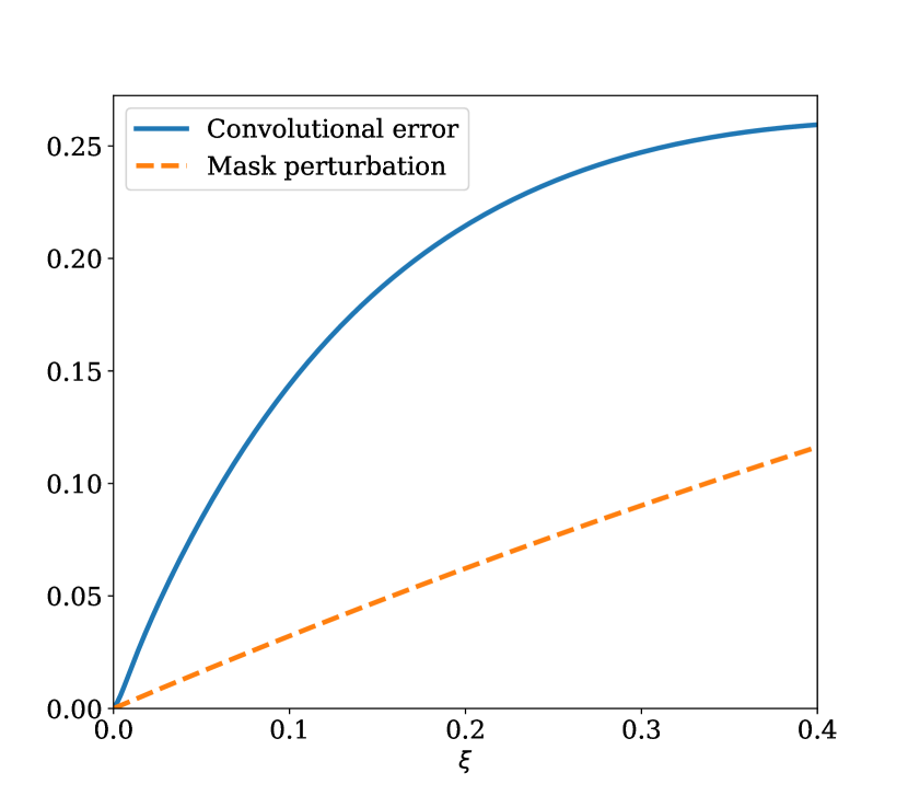
(d) Convolutional error.

Figure 5: Pseudo-reversing the subdivision scheme (31). Figure (5(a)) illustrates pushing the complex-valued zeros of (32) with a parameter $\xi$. The basic limit functions $\mathcal{S}_{\widetilde{\boldsymbol{\alpha}}}^{\infty}\boldsymbol{\delta}$ are depicted in Figure (5(c)). The decimation coefficients of $\mathcal{D}_{\boldsymbol{\gamma}}$ are illustrated in Figure (5(b)). Figure (5(d)) illustrates the convolutional error of (9), $\|\boldsymbol{\delta}-\boldsymbol{\gamma}*(\boldsymbol{\alpha}\downarrow 2)\|_{\infty}$, as well as the norm of the mask perturbation $\|\boldsymbol{\alpha}-\widetilde{\boldsymbol{\alpha}}\|_{\infty}$.

To shed more light on pseudo-reversing, Table 1 shows the reversibility condition $\kappa$ in (2) of $\widetilde{\boldsymbol{\alpha}}$ for different values of $\xi$, and for the same basic refinement. This table clearly shows the inverse correlation between $\xi$ and $\kappa$ as theory suggests in Corollary 2.6.

$\xi$	0	0.1	0.2	0.3	0.4	0.5	0.6	0.7	0.8	0.9	1	1.1	1.2
$\|\boldsymbol{\alpha}-\widetilde{\boldsymbol{\alpha}}\|_{\infty}$	0	0.03	0.06	0.09	0.11	0.14	0.16	0.18	0.20	0.22	0.23	0.25	0.26
$\kappa(\widetilde{\boldsymbol{\alpha}})$	$\infty$	18.19	9.54	6.67	5.24	4.38	3.81	3.41	3.11	2.88	2.69	2.54	2.41

Table 1: The mask perturbation and the reversibility condition of the approximating mask $\widetilde{\boldsymbol{\alpha}}$ against different parameters $\xi$.

As mentioned in Remark 3.2, the notion of pseudo-reversing can be relaxed and applied to refinements with bad reversibility conditions. That is, roughly speaking, schemes with zeros close to the unit circle. In other words, pseudo-reversing allows us to enforce a better, more practical reversibility. Technically, we can do this by pushing the zeros of $\boldsymbol{\alpha}(z)$ which have moduli greater than 1, with the factor $\xi$ as similar to (1).

Figure 6 illustrates the zeros of $\boldsymbol{\alpha}(z)$ in (10) and the coefficients of the solution $\boldsymbol{\gamma}$, where $\boldsymbol{\alpha}$ is the mask of a high order B-spline subdivision scheme. In addition, Table 2 shows the reversibility condition $\kappa$ of the reversible schemes, while Table 3 illustrates how pseudo-reversing imposes a better reversibility condition on the B-spline subdivision scheme of order 6.

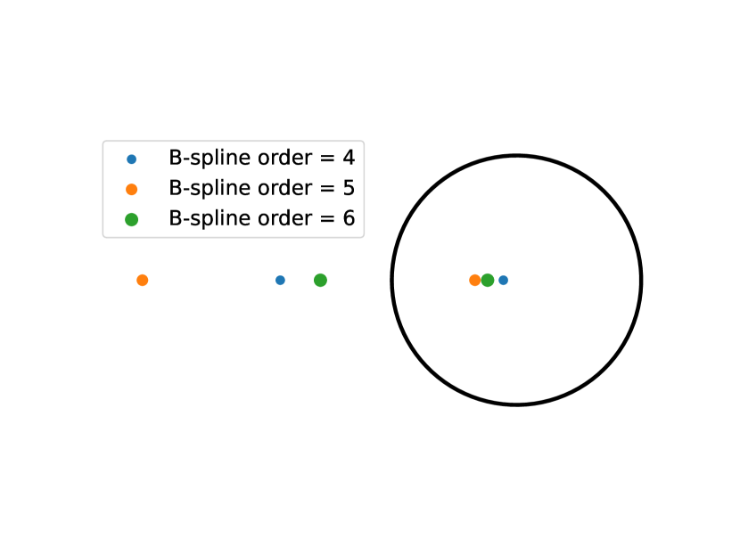
(a) Zeros of high order B-spline schemes.

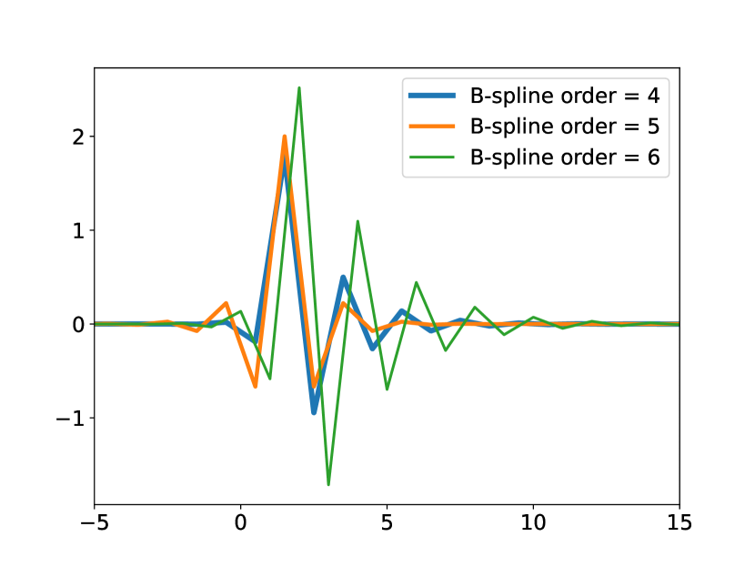
(b) Decimation coefficients.

Figure 6: Zeros and decimation coefficients of high order B-spline subdivision schemes. On the left, part of the zeros of $\boldsymbol{\alpha}(z)$ in (10) corresponding to the B-spline schemes of different orders, relative to $\mathbb{T}$. On the right, depiction of the corresponding decimation coefficients. Note how the minimal distance between the zeros and unit circle shrinks as the order increases (this holds for orders above 6 as well) and how the decay rate weakens as a result.

B-spline order	2	3	4	5	6	7
$\kappa(\boldsymbol{\alpha})$	2	2	4	4	8	8

Table 2: The reversibility condition (2) of the B-spline subdivision schemes. Note how the reversibility weakens as the order of the B-spline increases. Interestingly, the pattern seems to follow the rule $\kappa(\boldsymbol{\alpha})=2^{\lfloor n/2\rfloor}$ where $n$ is the B-spline order and $\left\lfloor\cdot\right\rfloor$ is the floor function. Also, the same value appears in the $2m$ and $2m+1$ orders because the symbol $\boldsymbol{\alpha}(z)=2^{-m}\sum_{j=0}^{\lfloor(m+1)/2\rfloor}\binom{m+1}{2j}z^{j}$.

$\xi$	0	0.1	0.2	0.3	0.4	0.5	0.6	0.7	0.8	0.9	1	1.1	1.2
$\kappa(\widetilde{\boldsymbol{\alpha}})$	8	6.59	5.69	5.06	4.60	4.25	3.97	3.74	3.55	3.39	3.26	3.14	3.04

Table 3: Improving the reversibility condition (2) of the B-spline subdivision scheme of order 6 with different parameters $\xi$. Only the zeros of $\boldsymbol{\alpha}(z)$ with moduli greater than 1 were displaced with the parameter $\xi$. Note how the reversibility improves as $\xi$ increases.

5.2 Multiscaling in the linear setting

Here we numerically illustrate the linear transform (12) and test the synthesis result appearing in Theorem 3.5. For this sake, we let $\boldsymbol{c}^{(6)}$ be our analyzed sequence, sampled from a test function $f(x):[0,10]\mapsto\mathbb{R}$ over the equispaced bounded grid $x\in 2^{-6}\mathbb{Z}\cap[0,10]$. We take $f$ to be the real part of the standard Morlet wavelet, centred at $x=5$.

We implement the pyramid transform (12) based on the subdivision scheme (31) and its pseudo-reverse $\mathcal{D}_{\boldsymbol{\gamma}}$ for $\xi=1.4$. We decompose the sequence $\boldsymbol{c}^{(6)}$ by iterating (12) $m$ times, for $m=1,2,\dots,6$, to get the pyramid $\{\boldsymbol{c}^{(6-m)};\boldsymbol{d}^{(5-m)},\dots,\boldsymbol{d}^{(6)}\}$. All detail coefficients on the even indices are then set to zero, yielding a sparser pyramid. Then, we reconstruct using the inverse pyramid transform. Theorem 3.5 suggests that the reconstruction error, measured by the infinity norm between the analyzed $\boldsymbol{c}^{(6)}$ and the reconstructed $\boldsymbol{\zeta}^{(6)}$ grows as $m$ increases. Reason being that, the more we decompose into coarse scales, the loss of information resulting from setting the even detail coefficients to zero becomes more significant, and hence the upper bound (17) increases – allowing more space for the error $\|\boldsymbol{c}^{(6)}-\boldsymbol{\zeta}^{(6)}\|_{\infty}$.

Figure 7 demonstrates the analyzed sequence $\boldsymbol{c}^{(6)}$ next to its $4$ layers ($m=4$) of detail coefficients. Note how the property of having small detail coefficients on the even indices is more pronounced on fine scales, and is violated on coarse scales. This phenomenon is explained via Theorem 3.4. The synthesis error is $0.1896$. Table 4 shows the synthesis error with respect to any number of layers $m$.

We finally remark here that similar results are obtained for any $\xi>0$, but we picked the value $\xi=1.4$ because it yielded a good reversibility condition $\kappa$ that was suitable for the truncation size of the decimation operator $\mathcal{D}_{\boldsymbol{\gamma}}$.

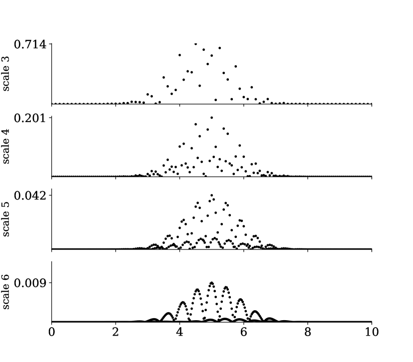
(a)

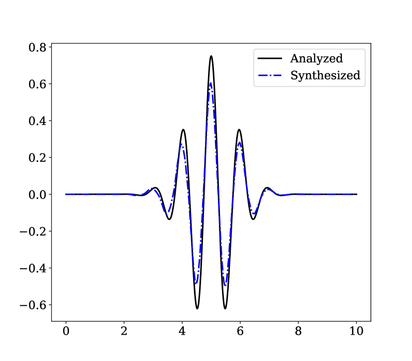
(b)

Figure 7: Linear multiscaling with a non-reversible subdivision scheme. On the right, the analyzed function in black, and the synthesized dot-dashed function in blue. On the left, the detail coefficients in absolute value of the first $4$ iterations of (12) for $\mathcal{S}_{\boldsymbol{\alpha}}$ of (31) and its pseudo-reverse $\mathcal{D}_{\boldsymbol{\gamma}}$ for $\xi=1.4$.

$m$	1	2	3	4	5	6
$\|\boldsymbol{c}^{(6)}-\boldsymbol{\zeta}^{(6)}\|_{\infty}$	0.0007	0.0059	0.0371	0.1896	0.3860	0.8816

Table 4: The reconstruction error against the number of detail layers.

5.3 Pyramid for SO(3) and manifold-valued contrast enhancement

We begin with an illustration of the multiscale transform (23) over the manifold of rotation matrices. That is, the rotation group $\text{SO}(3)$ acting on the Euclidean space $\mathbb{R}^{3}$. Then, we show the application of contrast enhancement using the multiscale representation.

Let

$$~{}\text{SO}(3)=\left\{R\in\mathbb{R}^{3\times 3}\;\big{|}\;R^{T}=R^{-1},\;\text{det}(R)=1\right\}$$ (33)

be the special orthogonal group consisting of all rotation matrices in $\mathbb{R}^{3}$. $\text{SO}(3)$ is endowed with a Riemannian manifold structure by considering it as a Riemannian submanifold of the embedding Euclidean space $\mathbb{R}^{3\times 3}$, with the inner product $\langle R_{1},R_{2}\rangle=\text{trace}(R_{1}^{T}R_{2})$ for $R_{1},R_{2}\in\text{SO}(3)$.

One simple way to generate smooth and random $\text{SO}(3)$-valued sequences to test our multiscaling (23) is to sample few rotation matrices, to associate the samples with indices, and then to refine using any refinement rule promising smooth limits, see e.g., [30]. Indeed, we followed this method to synthetically generate such a sequence. Specifically, we randomly generated $4$ rotation matrices, enriched the samples to $11$ matrices by a simple upsampling rule, and then refined the result using the cubic B-spline analogue (20) for few iterations. The resulted sequence is then parameterized over the dyadic grid $2^{-6}\mathbb{Z}$ corresponding to scale 6. In the refinement process, the Riemannian center of masses were approximated by the method of geodesic inductive averaging presented in [8].

To visualize the generated $\text{SO}(3)$-valued sequence, we rotate the standard orthonormal basis of $\mathbb{R}^{3}$ using each rotation matrix, and then depict all results on different locations depending on the parametrization as a time series. Figure 8(b) illustrates the result.

We now analyze the synthetic $\text{SO}(3)$-valued curve appearing in Figure 8(b) via the multiscale transform (23), using the nonlinear analogue $\mathcal{T}_{\boldsymbol{\alpha}}$ of the subdivision scheme (31), with its pseudo-reverse $\mathcal{Y}_{\boldsymbol{\gamma}}$ for $\xi=0.64$. The Riemannian center of masses (20) and (21) were approximated by the method of geodesic inductive averaging. Figure 8(a) exhibits the Frobenius norms of the first $4$ layers of detail coefficients. Note how the maximal norm of each layer can be bounded with geometrically decreasing values with respect to the scale. This indicates the smoothness of the curve. Moreover, the norms associated with the even indices are lower than the rest, this is a direct effect of $\boldsymbol{\gamma}$ truncation. Both phenomena were thoroughly explicated in [23]. Over and above, note how this effect is more pronounced on the high scales, this is explained in Lemma 4.1.

We remark here that the detail coefficients generated by the multiscale transform (23) lie in the tangent bundle $\bigcup_{R\in\text{SO}(3)}\left\{R\right\}\times T_{R}\text{SO}(3)$ where the tangent space $T_{R}\text{SO}(3)$ of a rotation matrix $R$ is the set of all matrices $RS\in\mathbb{R}^{3\times 3}$ where $S$ is skew-symmetric.

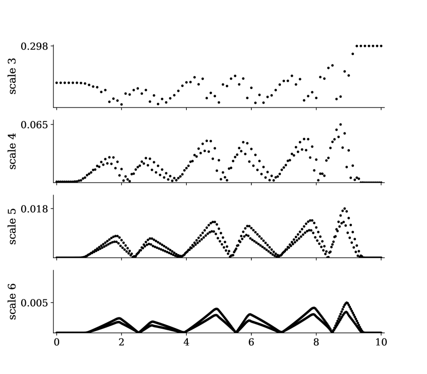
(a)

(b)

Figure 8: Multiscaling of $\text{SO}(3)$-valued sequence with a non-reversible subdivision scheme. On the right, visualization of a sequence of rotation matrices. On the left, the Frobenius norms of the first 4 layers of detail coefficients.

We now illustrate the application of contrast enhancement to the sequence in Figure 8(b) using its representation in Figure 8(a). In the context of multiscaling, the idea behind contrast enhancement lies in manipulating the detail coefficients while keeping the coarse approximation unchanged. Particularly, in order to add more contrast to a sequence, “swerves” in the case of rotations, one has to emphasize its most significant detail coefficients. Since all tangent spaces are closed under scalar multiplication, this can be done by multiplying the largest detail coefficients by a factor greater than $1$, while carefully monitoring the results to be within the injectivity radii of the manifold. The enhanced sequence is then synthesized from the modified pyramid.

Figure 9 shows the final result of enhancing the rotation sequence of Figure 8(b), side by side, where the largest 20% of the detail coefficients of each layer in Figure 8(a) were scaled up by 40%. Indeed, note how regions with small rotation changes are kept unchanged, while regions with high changes are more highlighted after the application. The specific percentages 20% and 40% were chosen to give good and convincing visual results.

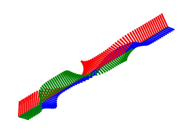
(a)

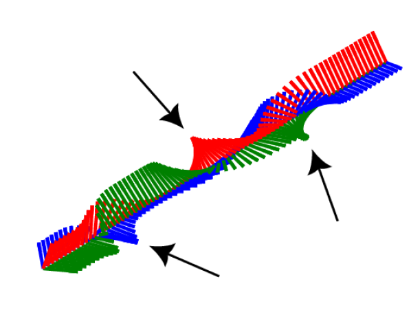
(b)

Figure 9: Contrast enhancement of SO(3)-valued sequence. On the left, the original sequence of rotation matrices. On the right, the enhanced rotation sequence. The largest 20% of the detail coefficients of each layer were enlarged by 40%. The black arrows indicate the regions with the most drastic twists – highlighting the effect of the application.

5.4 Data compression of rigid body motions

Here we consider the special Euclidean Lie group $\text{SE}(3)$ of dimension 6, which is the semidirect product of the special orthogonal group $\text{SO}(3)$ in (33) with the Euclidean space $\mathbb{R}^{3}$. Each element in this group makes a configuration of orientation and position to a rigid body. A convenient matrix representation of this group is

$$\text{SE}(3)=\text{SO}(3)\ltimes\mathbb{R}^{3}=\left\{\begin{pmatrix}R&p\\ 0&1\end{pmatrix}\bigg{|}\;R\in\text{SO}(3),\;p\in\mathbb{R}^{3}\right\}.$$

$\text{SE}(3)$ has a differentiable manifold structure in the embedding Euclidean space $\mathbb{R}^{4\times 4}$.

In this example, we take the $\text{SO}(3)$-valued curve appearing in Figure 8(b) and wrap it around a cone in $\mathbb{R}^{3}$, obtaining a time-series of location coordinates and orientations, i.e., a curve on $\text{SE}(3)$ parameterized over the equispaced grid $2^{-6}\mathbb{Z}$. Figure 10(a) depicts the curve and is often called a rigid body motion. We aim to compress this sequence via our multiscale transform.

We analyze the $\text{SE}(3)$-valued curve with the multiscale transform (23) using the nonlinear analogue $\mathcal{T}_{\boldsymbol{\alpha}}$ (20) of the subdivision scheme (31) with its pseudo-reverse $\mathcal{Y}_{\boldsymbol{\gamma}}$ of (21) for $\xi=0.64$. Specifically, we decompose the sequence four times to get the pyramid $\{\boldsymbol{c}^{(2)};\boldsymbol{d}^{(3)},\boldsymbol{d}^{(4)},\boldsymbol{d}^{(5)},\boldsymbol{d}^{(6)}\}$. The Riemannian center of masses (20) and (21) were approximated by the method of geodesic inductive averaging [8].

Similar to Section 5.2, we demonstrate the application of data compression by representing the ground-truth sequence on different scales, and then setting half of the detail coefficients to zero to get a sparser representation. Finally, we reconstruct using the inverse pyramid transform (24) and measure the error. The validity of the application lies in the ability to set half of the information of the multiscale representation to zero while maintaining visual resemblance to the original curve after synthesis with relatively low errors.

Figure 10 depicts the original sequence next to the synthesized compressed result. Note that if one chooses to use less details or decompose into more layers, the result is an increasing in the error of compression, as explained through Theorem 4.2. In the depicted example, we measure the error between the original sequence $\boldsymbol{c}^{(6)}$ and its estimation $\boldsymbol{\zeta}^{(6)}$ using a pointwise relative geodesic error, defined as

$${\mu^{r}}_{j}=\rho(\boldsymbol{c}^{(6)}_{j},\boldsymbol{\zeta}^{(6)}_{j})/\rho(\boldsymbol{c}^{(6)}_{j},e),$$ (34)

where $e$ is the identity of the group, represented by the $4\times 4$ identity matrix. In this example, we obtain that the median value of $\mu^{r}$ is $0.029$. The figure demonstrates that this low error rate is translated as almost identical sequences visually.

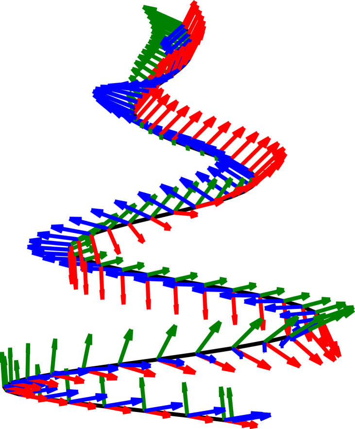
(a) Original SE(3) curve.

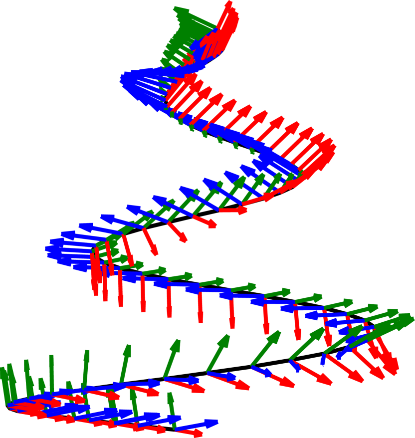
(b) Synthesized curve.

Figure 10: Compressing SE(3)-valued curve. On the left, depiction of the original ground-truth curve. On the right, the result of synthesizing, using just half of the available data. The difference between the two curves is visually noticeable mostly in the top and the bottom parts. The median of the relative error (34) is 2.9%.

Funding

NS is partially supported by the NSF-BSF award 2019752 and the DFG award 514588180.

References

- [1] Roberto Cavoretto. Adaptive radial basis function partition of unity interpolation: A bivariate algorithm for unstructured data. Journal of Scientific Computing, 87(2):41, 2021.
- [2] Rudrasis Chakraborty, Jose Bouza, Jonathan H Manton, and Baba C Vemuri. Manifoldnet: A deep neural network for manifold-valued data with applications. IEEE Transactions on Pattern Analysis and Machine Intelligence, 44(2):799–810, 2020.
- [3] Mariantonia Cotronei, Caroline Moosmüller, Tomas Sauer, and Nada Sissouno. Hermite multiwavelets for manifold-valued data. arXiv preprint arXiv:2110.10060, 2021.
- [4] Carl De Boor. A practical guide to splines, volume 27. springer-verlag New York, 1978.
- [5] Ramsay Dyer, Gert Vegter, and Mathijs Wintraecken. Barycentric coordinate neighbourhoods in riemannian manifolds. arXiv preprint arXiv:1606.01585, 2016.
- [6] Nira Dyn. Subdivision schemes in CAGD. Advances in numerical analysis, 2:36–104, 1992.
- [7] Nira Dyn, Allison Heard, Kai Hormann, and Nir Sharon. Univariate subdivision schemes for noisy data with geometric applications. Computer Aided Geometric Design, 37:85–104, 2015.
- [8] Nira Dyn and Nir Sharon. Manifold-valued subdivision schemes based on geodesic inductive averaging. Journal of Computational and Applied Mathematics, 311:54–67, 2017.
- [9] Jean Gallier, Jocelyn Quaintance, Jean Gallier, and Jocelyn Quaintance. Integration on manifolds. Differential Geometry and Lie Groups: A Second Course, pages 211–263, 2020.
- [10] Zhi Gao, Yuwei Wu, Mehrtash Harandi, and Yunde Jia. Curvature-adaptive meta-learning for fast adaptation to manifold data. IEEE Transactions on Pattern Analysis and Machine Intelligence, 45(2):1545–1562, 2022.
- [11] Karlheinz Gröchenig. Wiener’s lemma: theme and variations. an introduction to spectral invariance and its applications. In Four Short Courses on Harmonic Analysis, pages 175–234. Springer, 2010.
- [12] Philipp Grohs. Stability of manifold-valued subdivision schemes and multiscale transformations. Constructive approximation, 32:569–596, 2010.
- [13] Philipp Grohs and Johannes Wallner. Interpolatory wavelets for manifold-valued data. Applied and Computational Harmonic Analysis, 27(3):325–333, 2009.
- [14] Detlef Gromoll and Gerard Walschap. Metric foliations and curvature, volume 268. Springer Science & Business Media, 2009.
- [15] Karsten Grove and Hermann Karcher. How to conjugate C1-close group actions. Mathematische Zeitschrift, 132(1):11–20, 1973.
- [16] Hanne Hardering. Intrinsic discretization error bounds for geodesic finite elements. PhD thesis, FU Berlin, 2015.
- [17] Svenja Hüning and Johannes Wallner. Convergence analysis of subdivision processes on the sphere. IMA Journal of Numerical Analysis, 42(1):698–711, 2022.
- [18] Eberhard Kaniuth. A course in commutative Banach algebras, volume 16. Springer, 2009.
- [19] Hermann Karcher. Riemannian center of mass and mollifier smoothing. Communications on pure and applied mathematics, 30(5):509–541, 1977.
- [20] Hermann Karcher. Riemannian center of mass and so called Karcher mean. arXiv preprint arXiv:1407.2087, 2014.
- [21] Shoshichi Kobayashi and Katsumi Nomizu. Foundations of differential geometry, volume 1. New York, London, 1963.
- [22] Kanti V Mardia, Henrik Wiechers, Benjamin Eltzner, and Stephan F Huckemann. Principal component analysis and clustering on manifolds. Journal of Multivariate Analysis, 188:104862, 2022.
- [23] Wael Mattar and Nir Sharon. Pyramid transform of manifold data via subdivision operators. IMA Journal of Numerical Analysis, 2021.
- [24] Dyn N. and X Zhuang. Linear multiscale transforms based on even-reversible subdivision operators. In Excursions in Harmonic Analysis, volume 6. Springer, 2020.
- [25] DJ Newman. A simple proof of wiener’s theorem. Proceedings of the American Mathematical Society, 48(1):264–265, 1975.
- [26] Inam Ur Rahman, Iddo Drori, Victoria C Stodden, David L Donoho, and Peter Schröder. Multiscale representations for manifold-valued data. Multiscale Modeling & Simulation, 4(4):1201–1232, 2005.
- [27] Chafik Samir and Ines Adouani. C1 interpolating Bézier path on Riemannian manifolds, with applications to 3D shape space. Applied Mathematics and Computation, 348:371–384, 2019.
- [28] Oliver Sander. Geodesic finite elements of higher order. IMA Journal of Numerical Analysis, 36(1):238–266, 2016.
- [29] Thomas Strohmer. Four short stories about Toeplitz matrix calculations. Linear Algebra and its Applications, 343:321–344, 2002.
- [30] Johannes Wallner, Esfandiar Nava Yazdani, and Andreas Weinmann. Convergence and smoothness analysis of subdivision rules in riemannian and symmetric spaces. Advances in Computational Mathematics, 34:201–218, 2011.
- [31] Norbert Wiener. Tauberian theorems. Annals of mathematics, pages 1–100, 1932.