A 50 liter Cygno prototype overground characterization

Abstract

The nature of dark matter is still unknown and an experimental program to look for dark matter particles in our Galaxy should extend its sensitivity to light particles in the GeV mass range and exploit the directional information of the DM particle motion Vahsen:2020pzb . The Cygno project is studying a gaseous time projection chamber operated at atmospheric pressure with a Gas Electron Multiplier Sauli:1997qp amplification and with an optical readout as a promising technology for light dark matter and directional searches.

In this paper we describe the operation of a 50 liter prototype named LIME (Long Imaging ModulE) in an overground location at Laboratori Nazionali di Frascati of INFN. This prototype employs the technology under study for the 1 cubic meter Cygno demonstrator to be installed at the Laboratori Nazionali del Gran Sasso instruments6010006 . We report the characterization of LIME with photon sources in the energy range from few keV to several tens of keV to understand the performance of the energy reconstruction of the emitted electron. We achieved a low energy threshold of few keV and an energy resolution over the whole energy range of 10-20%, while operating the detector for several weeks continuously with very high operational efficiency. The energy spectrum of the reconstructed electrons is then reported and will be the basis to identify radio-contaminants of the LIME materials to be removed for future Cygno detectors.

1 Introduction

A number of astrophysical and cosmological observations are all consistent with the presence in the Universe of a large amount of matter with a very weak interaction with ordinary matter besides the gravitational force, universally known as Dark Matter (DM). The model of the Weakly Interacting Massive Particle (WIMP)) has been very popular in the last decades, predicting a possible DM candidate produced thermally at an early stage of the Universe with a mass in the range of 10 to 1000 GeV and a cross section of elastic scattering with standard matter at the level of that of the weak interactions bertone2005particle RevModPhys.90.045002 . Hypothetical particles of DM would also fill our Galaxy forming a halo of particles whose density profile is derived from the observed velocity distribution of stars in the Galaxy. This prediction calls for an experimental program for finding such DM particles with terrestrial experiments. These experiments aim at detecting the scattering of the elusive DM particle on the atoms of the detectors, inducing as experimental signature a nucleus or an electron to recoil against the impinging DM particle. Nowadays most of these experimental activities are based on ton (or multi-ton) mass detectors where scintillation light, ionization charge, or heat induced by the recoiling particles are used - sometime in combination - to detect the recoils XENON:2018voc ; aalbers2022dark ; Bernabei:2013xsa ; LUX:2016ggv ; PandaX-II:2017hlx .

Most of these experiments however are largely unable to infer the direction of motion of the impinging DM particle. While DM particles have a random direction in the Galaxy reference system. on the Earth a DM particle would be seen as moving along the direction of motion of the Earth in the Galaxy. This motion is given by the composition of the motion of the Sun toward the Cygnus constellation and the revolution and rotation of the Earth. This is then reflected into the average direction of motion of the recoiling particles after the DM scattering and it can represent an important signature to be exploited to discriminate the signal of a DM particle from other background sources MAYET20161 . Therefore this undoubtedly calls for a new class of detectors based on the reconstruction of the the recoil direction, such as the gaseous time projection chamber (TPC) Battat:2014van ; Battat:2016pap ; Battat:2016xxe ; BATTAT20146 ; Daw:2013waa ; Battat:2015rna ; bib:loomba55Fe ; JINST:nitec ; Ikeda:2020mvr ; Riffard:2016mgw ; Sauzet:2020dut ; Hashimoto:2017hlz ; BATTAT20151 ; ALNER2005173 ; bib:vahsen . Moreover, while the WIMP model for DM candidates has been tested thoroughly by the current detectors down to $10\text{\,}\mathrm{G}\mathrm{e}\mathrm{V}$, extensions of sensitivity of these detectors to lower masses - down to the GeV and below - are deemed fundamental to explore new models predicting lighter DM particles petraki2013review ; Zurek_2014 ; PhysRevLett.115.021301 . For this scope Cygno proposes the use of light atoms as Helium or Hydrogen as target for DM. For a DM in the range of 1 to $10\text{\,}\mathrm{G}\mathrm{e}\mathrm{V}$ mass the elastic scattering of DM particle on these nuclei is producing nuclear recoils with the most favourable kinetic energy.

In this respect the Cygno project aims to realize an R&D program to demonstrate the feasibility of a DM search based on gaseous TPC at atmospheric pressure. The Cygno TPC will use a He/CF₄ gas mixture featuring a GEM amplification and with an optical readout of the light emitted at the GEM amplification stage FRAGA200388 ; bib:Fraga as outlined in instruments6010006 . Gaseous TPC based on optical readout to search for DM were proposed and studied before but with the use of a gas pressure well below the atmospheric one (DM-TPC, Battat:2014mka ; Ahlen:2010ub ; DUJMIC2008327 ; PhysRevD.95.122002 ). The Cygno project aims to build a 30–100 $\text{\,}\mathrm{m}^{3}$ detector that would therefore host a larger target mass than a low pressure TPC. Given the presence of fluorine nuclei in the gas mixture Cygno would be especially sensitive to a scattering of DM that is sensitive to the spin of the nucleus. By profiting of the background rejection power of the directionality, competitive limits on the presence of DM in the Galaxy can be set, under the assumption of a spin dependent coupling of DM with matter.

After a series of explorative small size prototypes NIM:Marafinietal ; bib:jinst_orange1 ; bib:ieee_orange ; bib:nim_orange2 ; bib:jinst_orange2 ; Pinci:2019hhw ; Costa:2019tnu ; bib:fe55 ; bib:stab ; baracchini2019cygno proving the principle of detecting electron and nuclear recoils down to keV kinetic energy, a staged approach is now foreseen to build a detector sensitive to DM induced recoils.

A first step requires the demonstration that all the technological choices of the detector are viable. Before the construction a $1\text{\,}\mathrm{m}^{3}$ demonstrator of a DM Cygno-type detector, a 50 liter prototype - named LIME (Long Imaging ModulE) - has been built and operated in an overground laboratory at the Laboratori Nazionali di Frascati (LNF) of INFN. LIME is featuring a $50\text{\,}\mathrm{c}\mathrm{m}$ long drift volume with the amplification realized with a triple GEM system and the light produced in the avalanches readout with a scientific CMOS camera and four PMT. A Cygno-type detector will be modular with LIME being a prototype for one of its modules. Most of the materials and the detection elements used in LIME are not at the radiopurity level required for a real DM search. However they can be produced in a radiopure version, treated to become radiopure or replaced with radiopure materials without affecting the the mechanical feasibility and the detector performance of the $1\text{\,}\mathrm{m}^{3}$ Cygno demonstrator.

In this paper we summarize our experience with the LIME prototype operated during a long campaign of data-taking, conducted to primarily understand the long term operation stability, to collect data to develop image analysis techniques and to understand the particle energy reconstruction performance. These techniques are including the reconstruction of clusters of activated pixels due to light detection in the images, optical effects characterizations, and noise studies. They were mainly oriented to the detection of electron originated from the interaction of photons in the gas volume. We usually refer to these electrons as electron recoils. The energy response of LIME was fully characterized in a range of few keV to tens of keV electron kinetic energy using different photon sources, while a ⁵⁵Fe X-ray absorption length in the LIME gas mixture was also evaluated.

Finally we report an analysis of the observed background events, induced by sources both internal to the detector and external, in the overground LNF location.

2 The LIME prototype

The LIME prototype (as shown in Fig.1 and in Fig.2) is composed of a transparent acrylic vessel inside which the gas mixture is flowed with an over-pressure of about 3 mbar with respect to the external atmospheric pressure. Inside the gas vessel a series of copper rings are used as electrodes kept at increasing potential values from the cathode to define a uniform electric field directed orthogonal to the cathode plane. This field makes the ionization electrons (produced by the charged particles in the gas) to drift towards the anode. A cathode plane is used to define the lower potential of the electric field while on the opposite side a triple GEM stack system is installed. When the ionization electrons reach the GEM, they produce an avalanche of secondary electrons and ions. Interactions of secondary electrons with gas molecules produce also photons whose spectrum and quantity strongly depends on the gas mixture bib:Fraga . From the avalanche position the light is emitted towards the exterior of the vessel. A scientific CMOS camera (more details in Sect. 2.2) with a large field-of-view objective is used to collect this light over a integration time that can be set from $30\text{\,}\mathrm{m}\mathrm{s}$ to $10\text{\,}\mathrm{s}$ and to yield an image of the GEM. Four PMT are installed around the camera to detect the same light but with a much faster response time. In the following we describe in details the elements of the LIME prototype. The sensitive part of the gas volume of LIME is about 50 liters with a 50 cm long electric field region closed by a 33$\times$33 cm² triple-GEM stack.

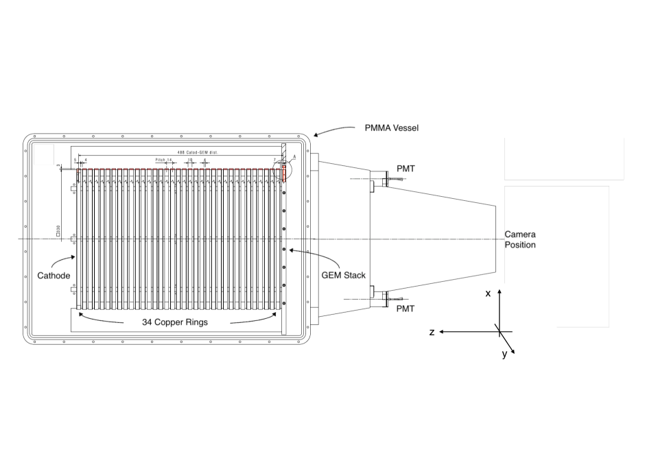
Figure 1: Drawing of LIME as seen from above. Square-shaped copper rings are used to create a field cage closed on one side by the triple-GEM stack. The field cage is closed on the other side with respect to the GEM by a cathode plane. The position of the four photomultipliers and of CMOS optical sensor are indicated. The acrylic gas vessel is enclosing the field cage and the GEM stack.

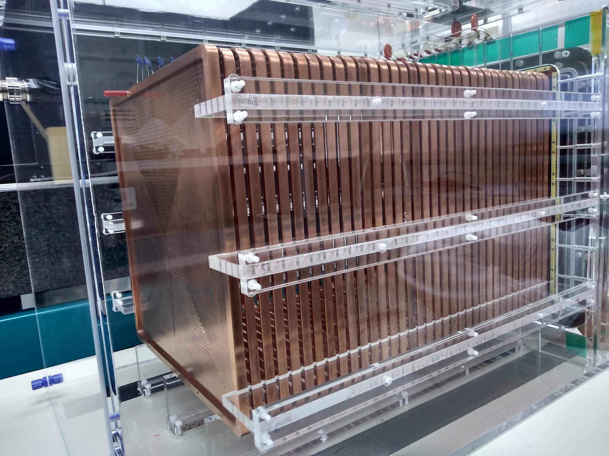
Figure 2: LIME vessel: the field cage is clearly visible with all its copper rings mounted on the PMMA combs to support them and with the cathode to close the field region.

2.1 The gas vessel and the field cage

The gas vessel is realized with a 10 mm thick PMMA box with a total volume of about 100 litres that is devoted to contain the gas mixture used in the operation. Inside the vessel a field cage produces a uniform electric field to drift the primary ionization electrons originated in the interaction of charged particles with the gas molecules towards the amplification stage. The volume is regularly flushed at a flow rate of $200\text{\,}\mathrm{c}\mathrm{c}\mathrm{/}\mathrm{m}\mathrm{i}\mathrm{n}$. The field cage has a square section, with a side of $330\text{\,}\mathrm{m}\mathrm{m}$, a length of $488\text{\,}\mathrm{m}\mathrm{m}$, and consists of:

• 34 square coils, $10\text{\,}\mathrm{m}\mathrm{m}$ wide, placed at a distance of $4\text{\,}\mathrm{m}\mathrm{m}$ from each other, with an effective pitch of $14\text{\,}\mathrm{m}\mathrm{m}$ and electrically connected by $100\text{\,}\mathrm{M}\Omega$ resistors;

• a $0.5\text{\,}\mathrm{m}\mathrm{m}$ thin copper cathode with a frame identical in size to the coils described above;

• a stack of 3 standard GEM (holes with an internal diameter of $50\text{\,}\mu\mathrm{m}$ and pitch of $140\text{\,}\mu\mathrm{m}$, placed $2\text{\,}\mathrm{m}\mathrm{m}$ apart from each other and $7\text{\,}\mathrm{m}\mathrm{m}$ from the first coils.

The detector is usually operated with a He/CF₄ gas mixture in proportions of 60/40 kept few millibars above the atmospheric pressure. This is therefore equivalent to a mass of 87 g in the active volume.

The upper face of the vessel includes a $5\text{\,}\mathrm{c}\mathrm{m}$ wide and $50\text{\,}\mathrm{c}\mathrm{m}$ long thin window sealed by a $150\text{\,}\mu\mathrm{m}$ thick ethylene-tetrafluoroethylene (ETFE) layer. This allows low energy photons (down to the keV energy) to enter the gas volume from external artificial radioactive sources used for calibration purposes.

An externally controllable trolley is mounted on the window and can be moved back and forth along a track. It functions as a source holder and allows to move a radioactive source, kept $18\text{\,}\mathrm{c}\mathrm{m}$ above the sensitive volume, along the $z$ axis from $5\text{\,}\mathrm{c}\mathrm{m}$ to $45\text{\,}\mathrm{c}\mathrm{m}$ far from the GEM. On its base there is a $5\text{\,}\mathrm{m}\mathrm{m}$ diameter hole that allows the passage of a beam of photons by collimating it.

The face of the vessel in front of the GEM stack away from the sensitive volume is $1\text{\,}\mathrm{m}\mathrm{m}$ thick to allow efficient transmission of light to the outside.

2.2 The light sensors

On the same side of the vessel where the GEM stack is installed a black PMMA conical structure is fixed to allow the housing of the optical sensors:

• 4 Hamamatsu R7378, 22 mm diameter photo-multipliers;

• an Orca Fusion scientific CMOS-based camera (more dentails on hamamatsu ) with 2304 $\times$ 2304 pixels with an active area of 6.5 $\times$ 6.5 $\mu$m² each, equipped with a Schneider lens with $25\text{\,}\mathrm{m}\mathrm{m}$ focal length and 0.95 aperture at a distance of $623\text{\,}\mathrm{m}\mathrm{m}$. The sCMOS sensor provides a quantum efficiency of about 80% in the range $450\text{\,}\mathrm{n}\mathrm{m}$-$630\text{\,}\mathrm{n}\mathrm{m}$. In this configuration, the sensor faces a surface of $35~{}\times~{}35$ cm² and therefore each pixel at an area of $152\times 152~{}\mu$m². The geometrical acceptance $\epsilon_{\Omega}$ results to be $1.2\times 10^{-4}$.

According to previous studies bib:Fraga ; bib:Margato1 , electro-luminescence spectra of He/CF₄ based mixtures show two main maxima: one around a wavelength of 300 nm and one around 620 nm. This second wavelength matches the range where the Fusion camera sensor provides thew maximum quantum efficiency.

2.3 The Faraday cage

The entire detector is contained within a 3 mm thick aluminium metal box. Equipped with feed-through connections for the high voltages required for the GEM, cathode and PMT and for the gas, this box acts as a Faraday cage and guarantees the light tightness of the detector. A rod is free to enter through a hole from the rear face to allow movement of the source holder. On the front side a square hole is present on which an optical bellows is mounted, which can then be coupled to the CMOS sensor lens.

2.4 Data acquisition and trigger systems

LIME data acquisition is realized with an integrated system within the Midas framework midas .

The PMT signals are sent into a discriminator and a logic module to produce a trigger signal based on a coincidence of the signals of at least two PMT.

A dedicated data acquisition PC is connected via two independent USB 3.0 ports to the camera and to a VME crate that houses I/O register modules for the trigger and controls.

The camera can be operated with different exposure times. The results presented in this paper are obtained with a 50 ms exposure to minimize the pile-up from natural radioactivity events.

The DAQ system has been designed and built in such a way that it can also integrate digitisers for the acquisition of PMT signal waveforms. In this way, for each interaction in the gas, the light produced in the GEM stack is simultaneously acquired by the high granularity CMOS sensor and by the four PMT. As it was demonstrated in bib:jinst_orange2 this will allow a 3D reconstruction of the event in the gas volume within the field cage.

In this paper we report the data analysis of the camera images only.

2.5 High voltage and gas supply systems

The gas mixture, obtained from cylinders of pure gases, is continuously flushed into the detector at a rate of 200 cc/min and the output gas is sent to an exhaust line connected to the external environment via a water filled bubbler ensuring the small (3 mbar) required overpressure. Electrical voltages at the various electrodes of the detector are supplied by two generators:

• an ISEG ”HPn 500” provides up to 50 kV and 7 mA with negative polarity and ripple $<0.2\%$ directly to the cathode;

• CAEN A1515TG board with Individual Floating Channels supplies the voltages (up to 1 kV with 20 mV precision) to the electrodes of the triple GEM stack

By means of these two suppliers, a constant electric field was generated in the sensitive volume with a standard value of E_Drift = 0.9 kV/cm and in the transfer gaps between the GEM (about E_Transf = 2.5 kV/cm), while the voltage difference across the two sides of each GEM is usually set to V_GEM = 440 V for all the three GEM.

3 Overground run

The measurements reported in this paper were realized at the INFN LNF during the 2021 summer and autumn. The detector was operated inside an experimental hall where the temperature was varying in a range between 295 K and 300 K and the atmospheric pressure between 970 and 1000 mbar for the entire duration of the measurements. The typical working conditions of the detector are reported in Table 1.

Table 1: Summary of the typical operating condition of LIME during the data takings.

Parameter	Typical value
Drift Field	0.9 kV/cm
GEM Voltage	440 V
Transfer Field	2.5 kV/cm
Gas Flow	12 l/h
PMT Threshold	15 mV

3.1 Instrumental effect studies

As a first study, we evaluated the instrumental non-uniformity due to the optics system and to the electronic sensor noise.

3.1.1 Optical vignetting

With respect to the optics, we evaluated the effects of lens vignetting, that is the reduction of detected light in the peripheral region of an image compared to the image center. For this purpose, we collected with the same camera images of a uniformly illuminated white surface. In order to avoid any possible preferiantial direction of the light impinging the sensor, different images of the same surface are acquired by rotating the camera around the lens optical axis, and we obtained a light collection map on the sensor by their average. This shows a drop of the collected light as a function of the radial distance from the centre, down to 20% with respect the center of the image, as shown in Fig. 3. The resulting map was then used to correct all the images collected with the detector.

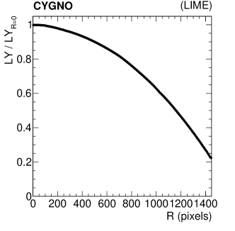
Figure 3: Light yield measured as a function of the radial distance from the center of the sensor, normalized to the one at the center, using pictures of a uniformly illuminated white surface.

3.1.2 Sensor electronic noise

A second study consisted in the evaluation of the fluctuations of the dark offset of the optical sensor. These are mainly due to two different contributions: readout noise i.e. the electronic noise of the amplifiers onboard of each pixel (less than 0.7 electrons r.m.s.) and a dark current that flows in each camera photo-diode of about 0.5 electrons/pixel/s hamamatsu2 . To obtain this, dedicated runs were taken throughout the data taking period with the values of V_GEM set to $200\text{\,}\mathrm{V}$. In this way the counts on the camera pixels were only due to the electronic noise of the sensor itself and not to any light. In each of these runs (called pedestal runs) we collected 100 images and we evaluated, pixel by pixel, the average value ($\text{\,}\mathrm{p}\mathrm{i}\mathrm{x}_{ped}$) and the standard deviation ($\text{\,}\mathrm{p}\mathrm{i}\mathrm{x}_{rms}$) of the response. The light tightness of the detector is ensured by the Faraday cage. To check its effectiveness, we compared the values of $\text{\,}\mathrm{p}\mathrm{i}\mathrm{x}_{ped}$ and $\text{\,}\mathrm{p}\mathrm{i}\mathrm{x}_{rms}$) in runs acquired with laboratory lights On and with completely dark laboratory without finding any significative differences.

In the reconstruction procedure, described later in Sec. 4.1, $\text{\,}\mathrm{p}\mathrm{i}\mathrm{x}_{ped}$ is then subtracted from the measured value, while $\text{\,}\mathrm{p}\mathrm{i}\mathrm{x}_{rms}$ is used to define the threshold to retain a pixel, i.e. when it has a number of counts larger than $1.1\text{\,}\mathrm{p}\mathrm{i}\mathrm{x}_{rms}$ .

The distribution of $\text{\,}\mathrm{p}\mathrm{i}\mathrm{x}_{rms}$ in one pedestal run for all the pixels of the sensor is shown in Fig. 4 (top). The long tail above the most probable value corresponds to pixels at the top and bottom boundaries of the sensor, which are slightly noisier than the wide central part. For this reason 250 pixel rows are excluded from the reconstruction at the top and 250 pixel rows at the bottom of the sensor. The stability of the pedestal value and of the electronics noise has been checked by considering the mean value of the distribution of $\text{\,}\mathrm{p}\mathrm{i}\mathrm{x}_{ped}$ and of $\text{\,}\mathrm{p}\mathrm{i}\mathrm{x}_{rms}$ as measured in the regular pedestal runs. Figure 4 middle and bottom show the distributions of the two quantities in a period of about two weeks, showing a very good stability of the sensor.

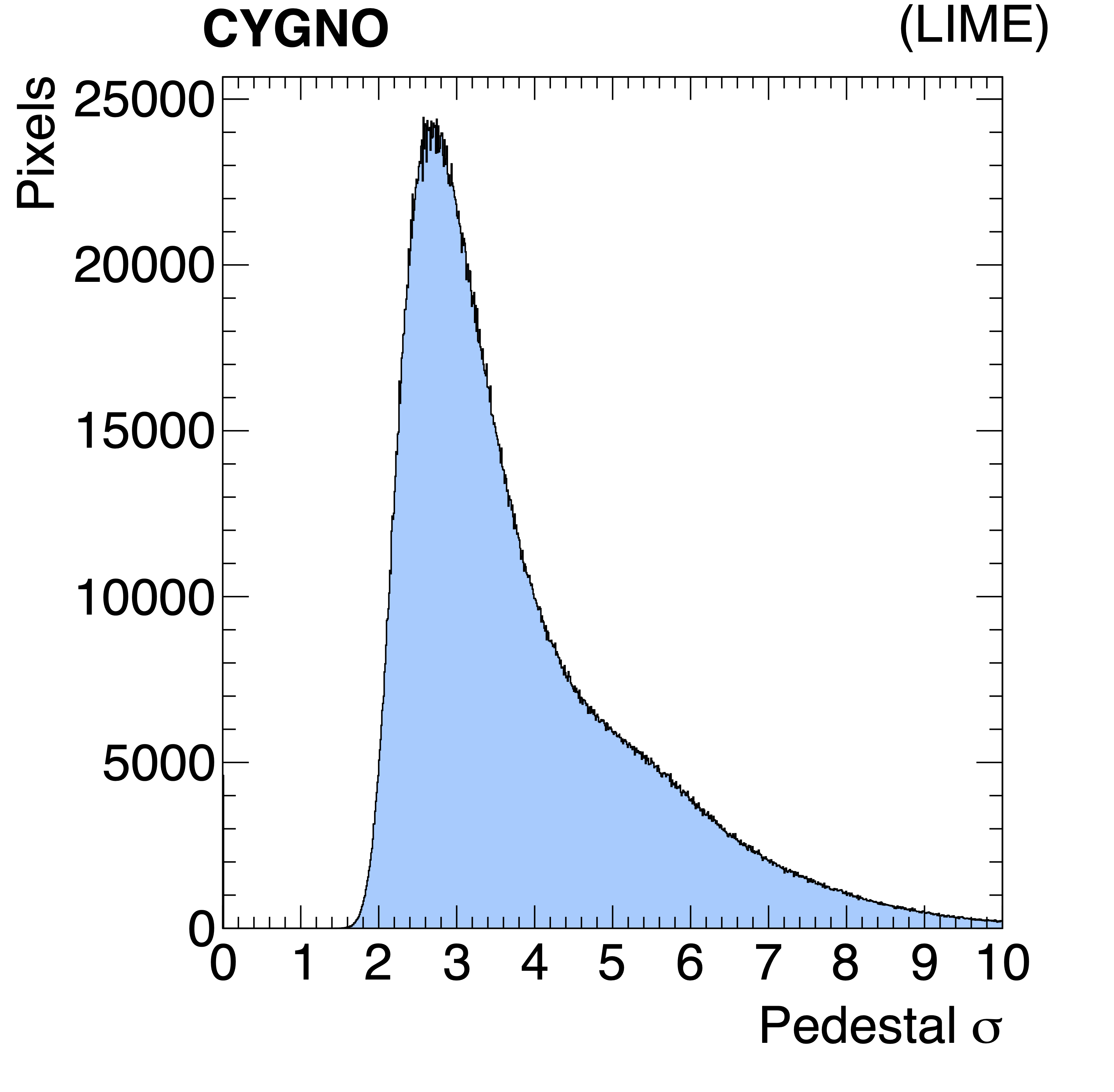
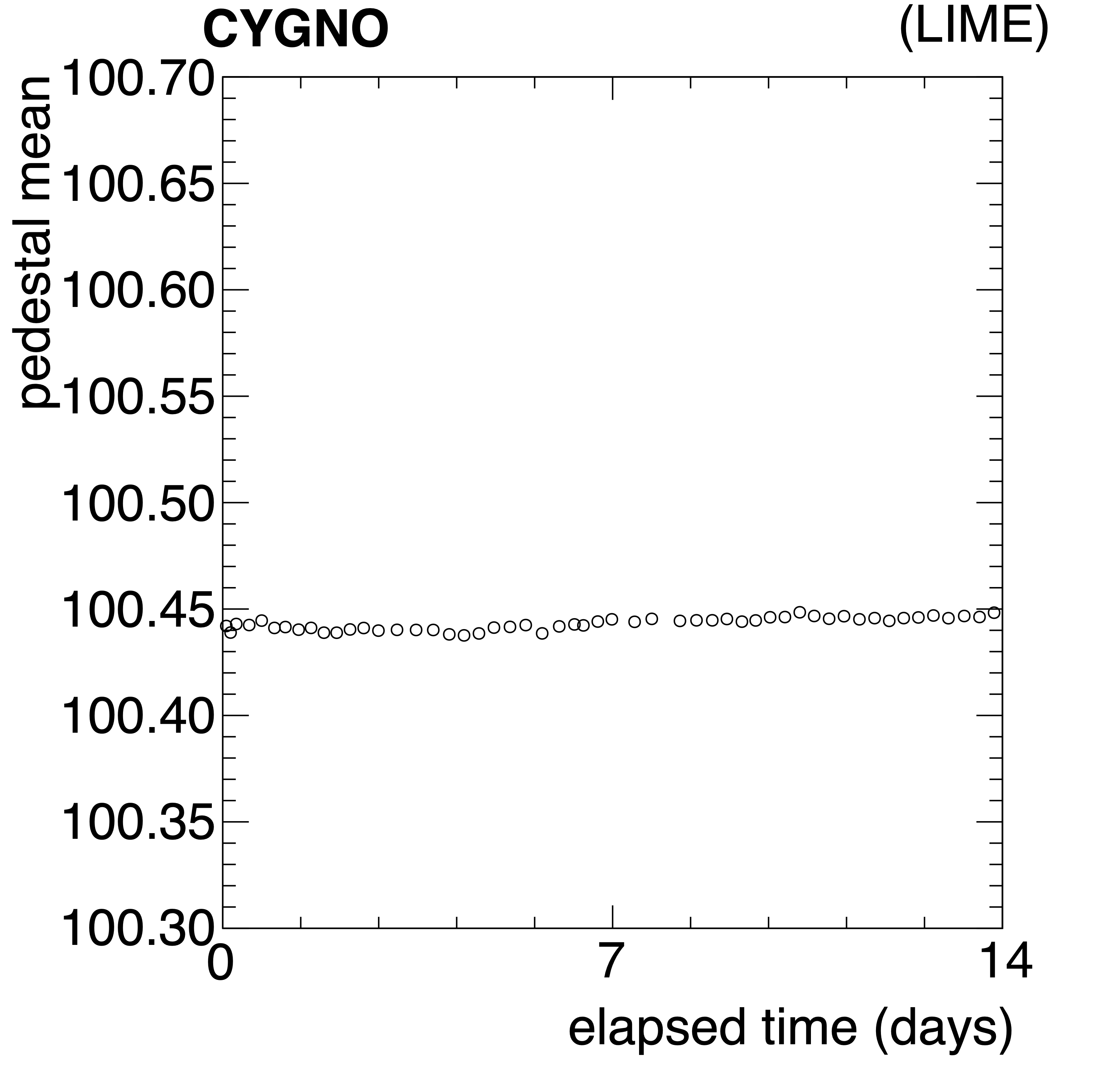
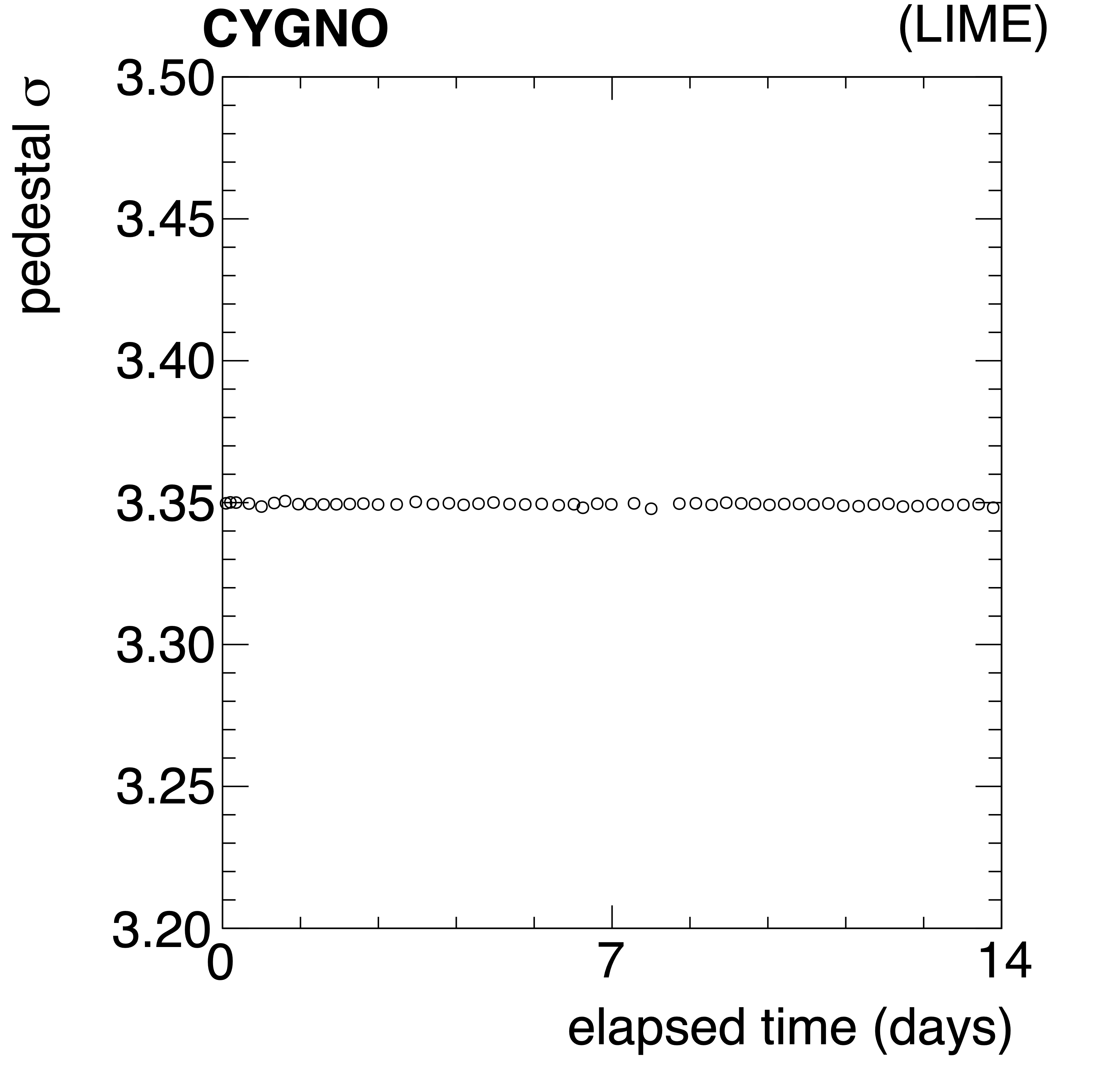
Figure 4: Top: distribution of pix${}_{\mbox{rms}}$ in one pedestal run. Middle and bottom: average of pix${}_{\mbox{ped}}$ and pix${}_{\mbox{rms}}$, respectively, as a function of time, for a period of two weeks of data taking, as measured in the regular pedestal runs acquired.

3.2 Electron recoils in LIME

A first standard characterization of the detector response to energy releases of the order of a few keV utilizes a ⁵⁵Fe source with an activity of $115\text{\,}\mathrm{M}\mathrm{B}\mathrm{q}$. ^55Fe decays by electron capture to an excited ^55Mn nucleus that de-excites by emitting X-rays with an energy of about $5.9\text{\,}\mathrm{k}\mathrm{e}\mathrm{V}$, with an additional emission at around $6.4\text{\,}\mathrm{k}\mathrm{e}\mathrm{V}$. Given the geometry of the source holder and trolley, the flux of the photons irradiates a cone with an aperture of about 10^∘. This means that in the central region of the detector, the flux is expected to have a gaussian transverse profile with a $\sigma$ of about $1\text{\,}\mathrm{c}\mathrm{m}$.

Moreover, in order to study the energy response for different X-rays energies, a compact multi-target source was employed Amersham . A sealed ²⁴¹Am primary source is selectively moved in front of different materials. Each material is presented to the primary source in turn and its characteristic X-ray is emitted through a 4 mm diameter aperture. In Tab. 2 a summary of the materials and energy of the X-ray lines is reported. The $K_{\beta}$ lines have an intensity that is about 20% of corresponding $K_{\alpha}$ lines.

Table 2: X-ray emitted by the multi-target source.

Material	Energy $K_{\alpha}$ [keV]	Energy $K_{\beta}$ [keV]
Cu	8.04	8.91
Rb	13.37	14.97
Mo	17.44	19.63
Ag	22.10	24.99
Ba	32.06	36.55

Given the physics interest to the detector response at low energies, the ^55Fe source X-rays with $E\approx$6\text{\,}\mathrm{k}\mathrm{e}\mathrm{V}$$ has been used to induce emissions of lower energy X-rays in two other targets: Ti and Ca. The expected $K_{\alpha}$ and $K_{\beta}$ lines are shown in Table 3. Given the experimental setup to excite the Ti and Ca lines, also the $6\text{\,}\mathrm{k}\mathrm{e}\mathrm{V}$ X-rays from ^55Fe can reach the detector active volume, resulting in the superposition of both contributions.

Table 3: X-ray emitted by the additional custom targets excited by the ^55Fe source.

Material	Energy $K_{\alpha}$ [keV]	Energy $K_{\beta}$ [keV]
Ti	4.51	4.93
Ca	3.69	4.01

The interaction of the X-ray with the gas molecules produces a electron recoil with a kinetic energy very similar to the X-ray energy. According to a SRIM simulation Ziegler1985 in our gas mixture at atmospheric pressure the expected range of the electron varies from about $250\text{\,}\mu\mathrm{m}$ for a $4\text{\,}\mathrm{k}\mathrm{e}\mathrm{V}$ energy to about $15\text{\,}\mathrm{m}\mathrm{m}$ for a $40\text{\,}\mathrm{k}\mathrm{e}\mathrm{V}$ energy instruments6010006 . These electron recoils produce a primary electron-ion pair at the cost of $42\text{\,}\mathrm{e}\mathrm{V}$ bib:rolandiblum ; bib:garfield ; bib:garfield1 Along the drift path longitudinal and transversal diffusion affect the primary ionization electrons distribution. Once they reach the GEM surface, these electrons start multiplication processes yielding an avalanche, producing at the same time also photons that are visible as tracks in the CMOS sensor image. These tracks from artificial radioactive sources are shown superimposed to tracks from natural radioactivity in a typical image ( Fig. 5). The tracks are reconstructed as 2D clusters of pixels by grouping the pixels with a non-null number of photons above the pedestal level.

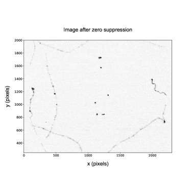
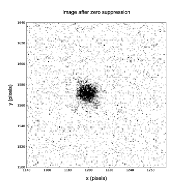
Figure 5: Example of an image with natural radioactivity tracks and luminous spots indicating the interactions in the gas of $6\text{\,}\mathrm{k}\mathrm{e}\mathrm{V}$ X-rays produced by the ^55Fe source. The ^55Fe source is located on the top of the sensitive volume and produces spots along the y axis (see Fig.1 for the reference frame) of the CMOS sensor (top). A zoom around one of these spots is also shown (bottom).

Once projected to the 2D GEM plane the spherical cloud of the drifting electrons from the ^55Fe X-ray interaction produces a $\approx$5\text{\,}\mathrm{m}\mathrm{m}$$ wide light profile along both the orthogonal axes of the cluster. The exact span of the profile depends on the running conditions of the detector and on the $z$ position of the X-ray interaction. In the following we refer to the longitudinal (transverse) direction as the orientation of the major (minor) axis of the cluster, found via a principal component analysis of the 2D cluster. The two profiles for a typical cluster are shown in Fig. 6 with a Gaussian fit superimposed. From these fits the values of $\sigma_{\mathrm{L}}$ and $\sigma_{\mathrm{T}}$ are obtained along with the amplitudes $A_{\mathrm{L}}$ and $A_{\mathrm{T}}$ respectively In general for non-spherical cluster due larger energy electron recoil we determine and utilizes only the $\sigma_{\mathrm{T}}$ value.

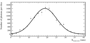
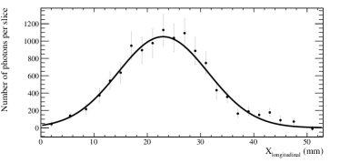
Figure 6: Example of transverse (top) and longitudinal (bottom) profiles of one luminous spot generated by the interactions in the gas of $6\text{\,}\mathrm{k}\mathrm{e}\mathrm{V}$ X-rays produced by the ^55Fe source. From the Gaussian fits the values of $\sigma_{\mathrm{T}}$ and $\sigma_{\mathrm{L}}$ are obtained along with the amplitudes $A_{\mathrm{T}}$ and $A_{\mathrm{L}}$ respectively.

4 Reconstruction of electron recoils

The energy deposit in the gas through ionization is estimated by clustering the light recorded in the camera image with a dynamic algorithm. The method is developed with the aim to be efficient with different topologies of deposits of light over the sensors. It is able to recognize small spots whose radius is determined by the diffusion in the gas, or long and straight tracks as the ones induced by cosmic rays traversing the whole detector, or long and curly tracks as the ones induced by various types of radioactivity. Radioactivity is in fact present in both the environment surrounding the detector or in the components of the detector itself.

4.1 The reconstruction algorithm

The reconstruction algorithm consists of four steps: (i) a zero suppression to reject the electronics noise of the sensor (ii) the correction for vignetting effect described in Sec. 3.1.1 and two steps of iterative clustering (iii) a super-clustering step to reconstruct long and smooth tracks parameterizing them as polynomial trajectories, and (iv) a small clustering step to find residual short deposits. The iterative approach is necessary for disentangling possibly overlapping long tracks recorded in the $50\text{\,}\mathrm{m}\mathrm{s}$ time interval of the exposure of the camera.

As a further noise reduction step, the resolution of the resulting image is initially reduced by forming macro-pixels, by averaging the counts in $4{\times}4$ pixel matrices, on which a median filter is applied, which is effective in suppressing the electronics noise fluctuations, as it is described in more details in Ref. coronello .

In order to first clean the picture from the long tracks originating from the ambient radioactivity, the iterative procedure of step (iii) is started, looking for possible candidate trajectories compatible with polynomial lines of increasing orders, ranging from 1 (straight line) to 3 as a generalization of the ransac algorithm ransac . If a good fit is found, then the supercluster is formed, and the pixels belonging to all the seed basic clusters are removed from the image, and the procedure is repeated with the remaining basic cluster seeds. The step (iii) is necessary to handle the cases of multiple overlaps of long tracks, as it can be seen in Fig. 7. It can be noticed that in the overlap region the energy is not shared, i.e. it is assigned to one of the overlapping tracks. In these cases the tracks can be split, but the pieces are still long enough not to mimick short deposits for low energy candidates of our interest for DM searches. When no more superclusters can be found, the superclustering stops, and the remaining pixels in the image are passed to step (iv), i.e. the search for small clusters. For this purpose, small-radius energy deposits are formed with Idbscan, described in details in Refs. iDBSCAN ; coronello . The effective gathering radius for pixels around a seed pixel is 5 pixel long, so small clusters are formed. Finally, the clusters from any iteration of the above procedure are merged in a unique collection, which form the track candidates set of the image.

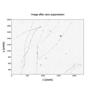
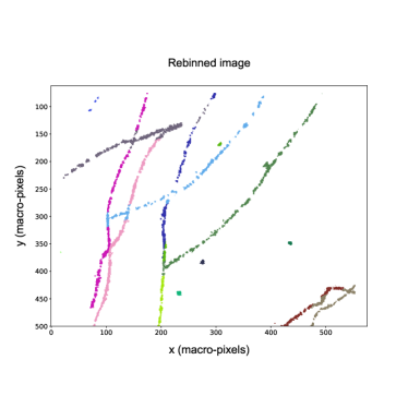
Figure 7: Top: image with an exposure of $50\text{\,}\mathrm{m}\mathrm{s}$. Bottom: reconstructed clusters after the two step procedure described in the text.

The track candidates are then characterized through the pattern of the 2D projection of the original 3D particle trajectory interacting within the TPC gas mixture. Various cluster shape variables are studied, and are useful to discriminate among different types of interactions coronello . For example a clear distinction can be made between tracks due to muons from cosmic rays and electron recoils due to X-rays. Moreover, within a given class of interactions, the cluster shapes are sensitive to the detector response, for example gas diffusion, electrical field non uniformities, gain non uniformities of the amplification stages. Thus they can be exploited to partially correct these instrumental effects improving the determination of the original interaction features, like the deposited energy, or its $z$-position, which cannot be directly inferred by the 2D information.

4.2 The ^55Fe source studies

The ^55Fe source is able to induce interaction in the gas mixture with an illumination of the entire vertical span of the detector as shown in Fig. 8. Due to the collimation of the source, only a slice in the horizontal direction has a significant occupancy of ^55Fe-induced clusters.

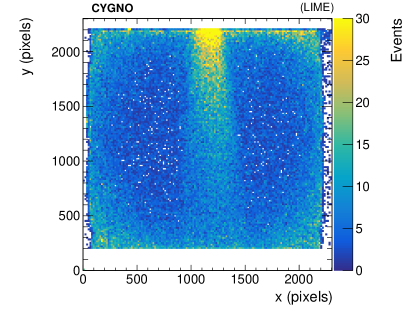
Figure 8: Spatial distribution of the reconstructed clusters in data collected with ^55Fe source. Only clusters in the central region of the GEM plane are selected to remove the noisier regions of the sensor. The ^55Fe source is positioned outside the detector at high values of $y$.

Several variables are used for the track characterization: $\sigma_{\mathrm{T}}$, the track length, the light density $\delta$ (defined as the integral of the light collected in the cluster, divided by the number of pixels over the noise threshold), the RMS of the light intensity residuals of the pixels $\text{\,}\mathrm{I}_{rms}$, and other variables described in more details in Ref. coronello .

A sample of clusters is obtained applying a very loose selection, which resembles the one optimized in Ref. coronello . Examples of the distributions for $\delta$ and for $\sigma_{\mathrm{T}}$ of these clusters are shown in Fig. 9, while the spectrum of $\text{\,}\mathrm{I}_{SC}$, defined as of the sum of the detected light in a cluster, is shown in Fig. 10 in a range below and around the expected deposit from the ^55Fe X-rays. The distribution of $\text{\,}\mathrm{I}_{SC}$ also shows a small enhancement at around twice the energy expected by the ^55Fe X-rays corresponding to the cases when two neighbor deposits are merged in a single cluster. This can happen because of the relatively large activity of the employed ^55Fe source. The average size of the spot produced by the ^55Fe X-ray interactions is about $20\text{\,}\mathrm{m}\mathrm{m}^{2}$.

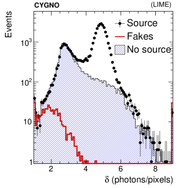
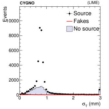
Figure 9: Top: light density $\delta$ in the reconstructed clusters, as defined in the text. Bottom: transverse dimension of the reconstructed cluster $\sigma_{\mathrm{T}}$. Black points represent data in presence of the ^55Fe source, filled histogram represents data without the source, while the red hollow histogram represents the contribution from mis-reconstructed clusters from electronics noise. The latter two are normalized to the live-time of the data taking with the ^55Fe source.

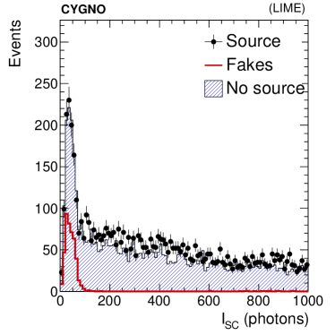
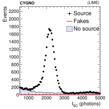
Figure 10: Light integral $\text{\,}\mathrm{I}_{SC}$ of the reconstructed clusters, as defined in the text. Top (bottom): region below (around) the expected energy peak from X-rays interactions from the ^55Fe source. Black points represent data in presence of the ^55Fe source, filled histogram represents data without the source, while the red hollow histogram represents the contribution from mis-reconstructed clusters from the electronics noise. The latter two are normalized to the live-time of the data taking with the ^55Fe source.

The distributions show the data obtained in data-taking runs both in presence of the X-ray source and without it, in order to show the background contribution, after normalizing them at the live-time of the data taking with the ^55Fe source. The expected contribution from fake clusters, defined as the clusters randomly reconstructed by neighboring pixels over the zero-suppression threshold, has been also estimated from the pedestal runs, where no signal contribution of any type is expected. As can be seen from Fig. 10 (top), this contribution becomes negligible for $\text{\,}\mathrm{I}_{SC}$$\gtrsim$400\text{\,}\mathrm{p}\mathrm{h}\mathrm{o}\mathrm{t}\mathrm{o}\mathrm{n}\mathrm{s}$$.

4.3 Energy calibration

Despite the correction of the optical effects of the camera applied before the clustering, the light yield associated to a cluster $\text{\,}\mathrm{I}_{SC}$ still depends on the position of the initial ionization site where the interaction within the active volume happened. Therefore the light yield $\text{\,}\mathrm{I}_{SC}$ must be converted in an energy $\text{\,}\mathrm{E}_{rec}$ by a calibration factor and then corrected to infer the original energy deposit E.

The $\text{\,}\mathrm{E}_{rec}$ dependence on the $x$–$y$ position of the initial interaction can be affected by possible imperfect correction of the vignetting effect, non uniformities of the drift field and of the amplification fields, especially near the periphery of the GEM planes, as shown in Fig. 11.

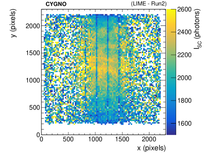
Figure 11: Average light yield, $\text{\,}\mathrm{I}_{SC}$, for the clusters as a function of the $x$–$y$ position in the 2D projection, for data collected with the ^55Fe source positioned at a $z=$26\text{\,}\mathrm{c}\mathrm{m}$$.

Moreover, inefficiency in the transport of the primary ionization electrons due to attachment during their drift in the gas would result in a monotonic decrease of $\text{\,}\mathrm{I}_{SC}$ as a function of $z$ of the initial interaction. However, as shown in Fig. 12, a continuous increase of $\text{\,}\mathrm{I}_{SC}$ with the $z$ of the initial interaction is observed.

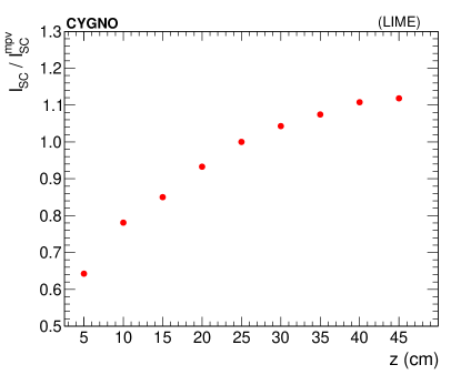
Figure 12: Average light yield, $\text{\,}\mathrm{I}_{SC}$, normalized to its most probable value, $\text{\,}\mathrm{I}_{SC}^{mpv}$, for clusters reconstructed in presence of the ^55Fe source as a function of the $z$ distance with respect the GEM planes.

This effect can be interpreted in the following way. During the amplification process, the channels across the GEM foils are filled with ions and electrons produced in the avalanches, but thanks to their small size they can rapidly drain. In recent years, however, several studies bib:highrate have shown that for high-gain (10⁶–10⁷) operations, the amount of charge produced by a single avalanche is already sufficient to change locally the electric field. In general this has the effect to reduce the effective gain of the GEM, causing a saturation effect. This also makes the response of the GEM system dependent on the amount of charge entering the channels and - in the case of many primary electrons from the gas ionization - on the size of the surface over which these electrons are distributed. In LIME, the diffusion of the primary ionization electrons over the 50 cm drift path can almost quadruple the size of the surface involved in the multiplication, thus reducing the charge density and therefore reducing the effect of a gain decrease.

We think this to be the cause of the observed behavior of the spots originated by the ^55Fe X-rays over the whole drift region: the light yield $\text{\,}\mathrm{I}_{SC}$ for spots originated by interactions farther from the GEM is larger than for spots closer to the GEM. Thus, the overall trend of $\text{\,}\mathrm{I}_{SC}$ as a function of the $z$ position of the ionisation site therefore presents an initial growth followed by an almost plateau region, as shown in Fig. 12.

These effects partially impact the observed cluster shapes. However, they can be used as a handle, together with the $x$–$y$ measured position in the 2D plane, to infer E. Since multiple effects impact different variables in a correlated way, corrections for the non perfect response to the true energy deposits have been optimized using a multivariate regression technique, also denoted as multivariate analysis (MVA), based on a Boosted Decision Tree (BDT) implementation, following a strategy used in Ref. cmsecal .

The training has then been performed on data recorded with the various X-rays deposits described in Table 2 and Table 3. The target variable of the regression is the mean value of the ratio $\text{\,}\mathrm{I}_{SC}$$/$\text{\,}\mathrm{I}_{SC}^{mpv}$$, where the most probable value $\text{\,}\mathrm{I}_{SC}^{mpv}$ is the most probable value of the $\text{\,}\mathrm{I}_{SC}$ distribution for each radioactive source. The performance of the regression using the median of the distribution instead of the mean have been checked and found giving a negligible difference.

The clusters were selected by requiring their $\sigma_{\mathrm{T}}$ to be consistent with the effect of the diffusion in the gas and their length not larger than what is expected for an X-ray of energy E. In addition it is required that $\text{\,}\mathrm{I}_{SC}$ falls within $5\,\sigma_{G}$ from the expected E for a given source, where $\sigma_{G}$ is the measured standard deviation of the peak in the $\text{\,}\mathrm{I}_{SC}$ distribution (estimated through a Gaussian fit). The background contamination of the training samples after selection, estimated by applying the selection on the data without any source, is within 1–5% of the total number of selected clusters.

The input variables to the regression algorithm are the $x$ and $y$ coordinates of the supercluster, and a set of cluster shape variables, among which the most relevant are the ratio $\frac{\sigma_{\mathrm{T}}}{A_{\mathrm{T}}}$, $\text{\,}\mathrm{I}_{rms}$ and $\delta$. Variables that are proportional to $\text{\,}\mathrm{I}_{SC}$ are explicitly removed, in order to derive a correction which is as independent as possible on the true energy E. In order to be sensitive to the variation of the inputs variables as a function of $z$, and possibly correct for the saturation effect, data with the ^55Fe source have been collected with the source positioned at different values of $z$ uniformly distributed, with a step of $5\text{\,}\mathrm{c}\mathrm{m}$ from the GEM to the cathode. The data collected with the other sources of Tables 2 and 3 instead were only taken at $z=$26\text{\,}\mathrm{c}\mathrm{m}$$.

A sanity check on the output of the regression algorithm is performed on the data without any source, where the energy spectrum of the reconstructed clusters extends over the full set of $K_{\alpha}$ and $K_{\beta}$ lines used for the training. No bias or spurious bumps induced by the training using only few discrete energy points is observed.

The $K_{\alpha}$ line expected for the ^55Fe X-rays, when the source is positioned at $z=$26\text{\,}\mathrm{c}\mathrm{m}$$, is used to derive the absolute energy calibration conversion, which equals is approximately $\kappa~{}=~{}$0.38\text{\,}\mathrm{p}\mathrm{h}\mathrm{o}\mathrm{t}\mathrm{o}\mathrm{n}\mathrm{s}\mathrm{/}\mathrm{e}\mathrm{V}$$. The absolute reconstructed raw energy is thus defined as $$\text{\,}\mathrm{E}_{rec}$~{}=~{}$$\text{\,}\mathrm{I}_{SC}$$\,/\,\kappa$. The absolute energy, after the multivariate regression correction described above, is denoted as E in the following.

The comparison of the distributions for the raw supercluster energy, $\text{\,}\mathrm{E}_{rec}$, and E, using data collected in presence of the ^55Fe radioactive source is shown in Fig. 13 for two extreme distances from the GEM planes, $z=$11\text{\,}\mathrm{c}\mathrm{m}$$ and $z=$41\text{\,}\mathrm{c}\mathrm{m}$$. The improvement in the energy resolution is substantial. The distribution after the correction shows a small tail below the most probable value of the distribution, indicating a residual non-perfect containment of the cluster, that systematically underestimates the energy and should be corrected by improving the cluster reconstruction.

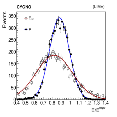
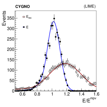
Figure 13: Comparison between $\text{\,}\mathrm{E}_{rec}$ (open squares) and E (filled circles) normalized by the most probable value of the corresponding distribution for $z=$26\text{\,}\mathrm{c}\mathrm{m}$$, on data collected with ^55Fe source at a distance of $z=$11\text{\,}\mathrm{c}\mathrm{m}$$ (top) or $z=$41\text{\,}\mathrm{c}\mathrm{m}$$ (bottom) from the GEM planes. A fit with a Crystal Ball function, as discribed in the text, is superimposed to each distribution.

The efficacy of the MVA regression in correcting for the saturation effect and other response non uniformities is estimated with the data sample collected with ^55Fe source. The $$\text{\,}\mathrm{E}_{rec}$/$\text{\,}\mathrm{E}_{rec}^{mpv}$$ and E/$\text{\,}\mathrm{E}^{mpv}$ distributions are fit with a Crystal Ball function CrystalBall , which describes their tails: $f(E;m_{G},\sigma_{G},\alpha,n)$, where the parameters $m_{G}$ and $\sigma_{G}$ describe the mean and standard deviation of the Gaussian core, respectively, while the parameters $\alpha$ and $n$ describe the tail.

The average response is estimated with the fitted value of $m_{G}$. Its value, as a function of the $z$ position, is shown in Fig. 14 (top). The effect of the saturation is only partially corrected through this procedure: the consequence of the gain loss is reduced by about 15% in correspondence of the smallest distance tested, $z=$5\text{\,}\mathrm{c}\mathrm{m}$$. Yet, this small improvement indicates that it is possible to roughly infer the $z$ position through a similar regression technique, where the target variable is $z$, instead of E. This procedure will be discussed in Sec. 5. The same procedure, applied on data samples with variable energy and variable $z$ position, would allow to build the model of the correction with larger sensitivity to $z$, thus resulting in an improved correction of the saturation effect.

On the other hand, it is evident that the MVA regression improves the energy resolution for any $z$, by correcting effects distinct from the saturation. The standard deviation of the Gaussian core of the distribution is estimated by $\sigma_{G}$, representing the resolution of the best clusters. Clusters belonging to the tails of the distribution, for which the corrections are suboptimal, slightly worsen the average resolution. Its effective value for the whole sample is then estimated with the standard deviation of the full distribution. The values of both estimators are shown in Fig. 14 as a function of the $z$ position of the ^55Fe source: for the clusters less affected by the saturation ($z\gtrsim$15\text{\,}\mathrm{c}\mathrm{m}$$) the RMS value improves from $\approx 20\%$ to $\approx 12\%$. The best clusters, whose resolution is estimated with $\sigma_{G}$, have a resolution smaller than $10\%$ for $z\gtrsim$25\text{\,}\mathrm{c}\mathrm{m}$$, when the saturation effect is small.

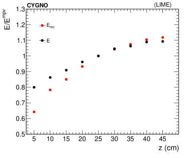
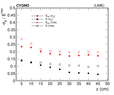
Figure 14: Top: average energy response to X-rays from ^55Fe source, normalized to the most probable value of the distribution of the sample with $z=$26\text{\,}\mathrm{c}\mathrm{m}$$, estimated from the raw supercluster energy $\text{\,}\mathrm{E}_{rec}$ (red points) and including the correction with the MVA regression, E (black points), as a function of the $z$ distance from the GEM planes. Bottom: energy resolution in the same data, estimated either as the RMS of the full distribution (open squares) or from the fitted $\sigma_{G}$ of the Crystal Ball function described in the text (filled circles), as a function of the $z$ distance from the GEM planes.

4.4 Study of the response linearity

The energy response of the detector as a function of the impinging X-ray energy is studied by selecting clusters reconstructed in presence of the different radioactive sources enumerated in Table 2, in addition to the large data sample recorded with the ^55Fe source positioned at the same distance from the GEM plane. The data used were recorded placing the radioactive source at $z=$25\text{\,}\mathrm{c}\mathrm{m}$$. The average energy response of the latter is used to derive the absolute energy scale calibration constant. The distributions of the cluster energy E, for the data collected with any of the radioactive sources used, are shown in Fig. 15. The samples are selected with a common loose preselection, and the spectra, normalized to the live-time, are compared to the one measured in data acquired without any source. This proves that the shape of the background is common to all the data samples, thus will be estimated from this control sample in what follows.

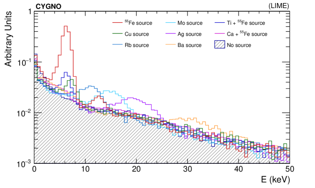
Figure 15: Spectra of the calibrated energy E for data collected in presence of the radioactive sources, placed at $z=$25\text{\,}\mathrm{c}\mathrm{m}$$, listed in Table 2, compared to the spectrum of clusters reconstructed in a data sample without any source. The distributions are normalized to the same live-time.

For each data sample a loose cluster selection, slightly optimized for each source with respect to the loose common preselection, is applied to increase the signal over background ratio. As it is shown in Fig. 10, the energy spectrum of the underlying background from natural radioactivity deposits is in general a smoothly falling distribution, while the response to fixed-energy X-rays is a peak whose position represents the mean response to that deposit, while the standard deviation is fully dominated by the experimental energy resolution. Deviations from a simple Gaussian distribution are expected especially as an exponential tail below the peak, due to non perfect containment of the energy in the reconstructed clusters.

The average energy response is estimated through a fit of the energy distribution, calibrated using the one to the ^55Fe source, using two components: one accounting for the non-peaking background from natural radioactivity, and one for true X-rays deposits. The background shape is modeled through a sum of Bernstein polynomials bernstein of order $n$, with $n=[1\dots 5]$: the value of $n$ and its coefficients are found fitting the energy distribution of clusters selected on data without the ^55Fe source. The value of $n$ is chosen as the one giving the minimum reduced $\chi^{2}$ in such a fit. The signal shape is fitted using the sum of two Cruijff functions, each of one is a centered Gaussian with different left-right standard deviations and exponential tails cruijff . The two functions represent the contribution of the $K_{\alpha}$ and $K_{\beta}$ lines listed in Table 2: the energy difference between the two (denoted main line and $2^{nd}$ line in the figures) is fixed to the expected value, thus in each fit only one scale parameter is fully floating. The remaining shape parameters of the Cruijff functions are constrained to be the same for the two contributions, since they represent the experimental resolution which is expected to be the same for two similar energy values. While the energy difference between the main and subleading line are well known, the relative fraction of the two contributions $f_{2}$ also depends on the absorption rate of low energy X-rays by the detector walls, so it is left floating in the fit, with the constraint $f_{2}<0.3$. In particular the ^55Fe source was separately charatecterized with with a Silicon Drift Detectors with about $100\text{\,}\mathrm{e}\mathrm{V}$ resolution on the energy and the fraction of $K_{\beta}$ transitions was found to be 18%. In the case of the Rb target, the range of energy of the reconstructed clusters covers the region of possible X-rays induced by the ²⁴¹Am primary source impinging the copper rings constituting the field cage of the detector. Thus a line corresponding to Cu characteristic energy is added: its peak position is constrained to the main Rb $K_{\alpha}$ line fixing the energy difference $\Delta E=K_{\alpha}^{\ce{Rb}}-K_{\alpha}^{\ce{Cu}}$ to the expected value. Since only a small contribution is expected from Cu with respect the main Rb one, no $K_{\beta}^{\ce{Rb}}$ is added. The normalization of the Cu component is left completely floating.

The response to X-rays with lower energies than the $6\text{\,}\mathrm{k}\mathrm{e}\mathrm{V}$ emitted by ^55Fe have been tested with the Ti and Ca targets listed in Table 3. As discussed earlier, in this setup an unknown fraction of the original $6\text{\,}\mathrm{k}\mathrm{e}\mathrm{V}$ X-rays also pass through the target, so the fit to the energy spectrum is performed addding to the total likelihood also the two-components PDF expected from ^55Fe contribution. While the shape for the four expected energy lines is constrained to be the same, except the mean values and the resolution parameters, the relative normalization is kept floating. The shape of the natural radioactivity background is fixed to the one fitted on the data collected without source.

Example of the fits to the energy spectra in the data with different X-ray sources are shown in Fig. 16 and Fig. 17.

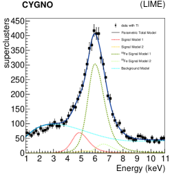
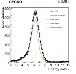
Figure 16: Energy spectra of reconstructed clusters in presence of different X-ray sources. Top: Ti source. Bottom: ^55Fe source (used also to estimate the absolute energy scale calibration throughout the paper). Blue dotted line represents the background shape, modelled on data without any source; red dotted line represent the $K_{\alpha}$ line signal model; red dotted line represents the $K_{\beta}$ line signal model. The blue continuous line represents the total fit function.

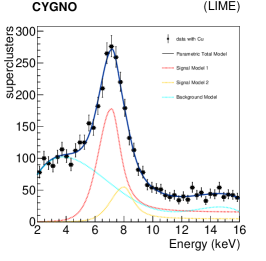
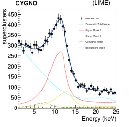
Figure 17: Energy spectra of reconstructed clusters in presence of different X-ray sources. Top: Cu source. Bottom: Rb source. Ag source. Bottom: Ba source. Blue dotted line represents the background shape, modelled on data without any source; red dotted line represent the $K_{\alpha}$ line signal model; red dotted line represents the $K_{\beta}$ line signal model. The blue continuous line represents the total fit function. As explained in the text, for the Rb target, a component from the expected contribution of Cu induced X-rays is added, represented by the green dashed line.

The estimated energy response from these fits, compared to the expected X-ray energy for each source is shown in Fig. 18. In the graph the contributions from both $K_{\alpha}$ and $K_{\beta}$ lines are shown, because both components are used in the minimization for the energy scale in each fit. The two values are correlated by construction of the fit model. A systematic uncertainty to the fitted value is considered, originating from the knowledge of the $z$ position of the source. Because of the effect described in Sec. 4.2, a change in this coordinate results in a change of the light yield: with the source positioned at $z\approx$21\text{\,}\mathrm{c}\mathrm{m}$$, data with ^55Fe source (shown in Fig. 14) allow to estimate a variation $\Delta E/\Delta z\approx 2\%/$1\text{\,}\mathrm{c}\mathrm{m}$$. An uncertainty $\Delta z=$1\text{\,}\mathrm{c}\mathrm{m}$$ is assumed for the position of the X-ray source, and the resulting energy uncertainty is added in quadrature to the statistical one from the fit.

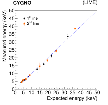
Figure 18: Estimated average energy response versus the expected one from the $K_{\alpha}$ (black dots) or $K_{\beta}$ lines contributions. The uncertainties on each point represent the statistical contribution and the systematic uncertainty arising from the knowledge of the $z$ position. The dotted line represents the a perfect linear response of the detector.

5 Evaluation of the $z$ coordinate of the ionization point

The ability to reconstruct the three-dimensional position in space of events within the detector allows, as has been shown in Daw:2013waa , the rejection of those events too close to the edges of the sensitive volume and therefore probably due to radioactivity in the detector materials (GEM, cathode, field cage). As shown in other work, the optical readout allows submillimeter accuracy in reconstructing the position of the spots $x$–$y$ plane NIM:Marafinietal ; bib:jinst_orange1 . The $z$ coordinate can be evaluated by exploiting the effects of electron diffusion in the gas during the drift path. The diffusion changes the distribution in space of the electrons in the cluster produced by the ionization and therefore it modifies the shape of the light spot produced by the GEM and collected by the CMOS sensor. Based on this, a simple method was developed for ultra-relativistic particle tracks bib:relativistic , relying on $\sigma_{T}$ (see for example  Fig. 6).

We evaluated the $z$-reconstruction performance by studying the behavior of several shape variables of the spots produced by the ^55Fe source, and therefore at a fixed energy, as a function of the $z$ coordinate of the source (z${}_{\ce{{}^{55}Fe}}$ in the following).

The variable that showed a better performance is $\zeta$ defined as the product of the gaussian sigma fitted to transverse profile of the spots (see Fig. 6) $\sigma_{T}$ and the standard deviation of the counts per pixel inside the spots $\text{\,}\mathrm{I}_{rms}$. Figure 19 shows on the left the distribution of $\zeta$ of all reconstructed spots as a function of nine values of z${}_{\ce{{}^{55}Fe}}$ (in the range from $5\text{\,}\mathrm{c}\mathrm{m}$ to $45\text{\,}\mathrm{c}\mathrm{m}$). For each value of z${}_{\ce{{}^{55}Fe}}$ the mean value of the distribution of $\zeta$ is superimposed together with a quadratic fit to the trend of these averages as a function of z${}_{\ce{{}^{55}Fe}}$.

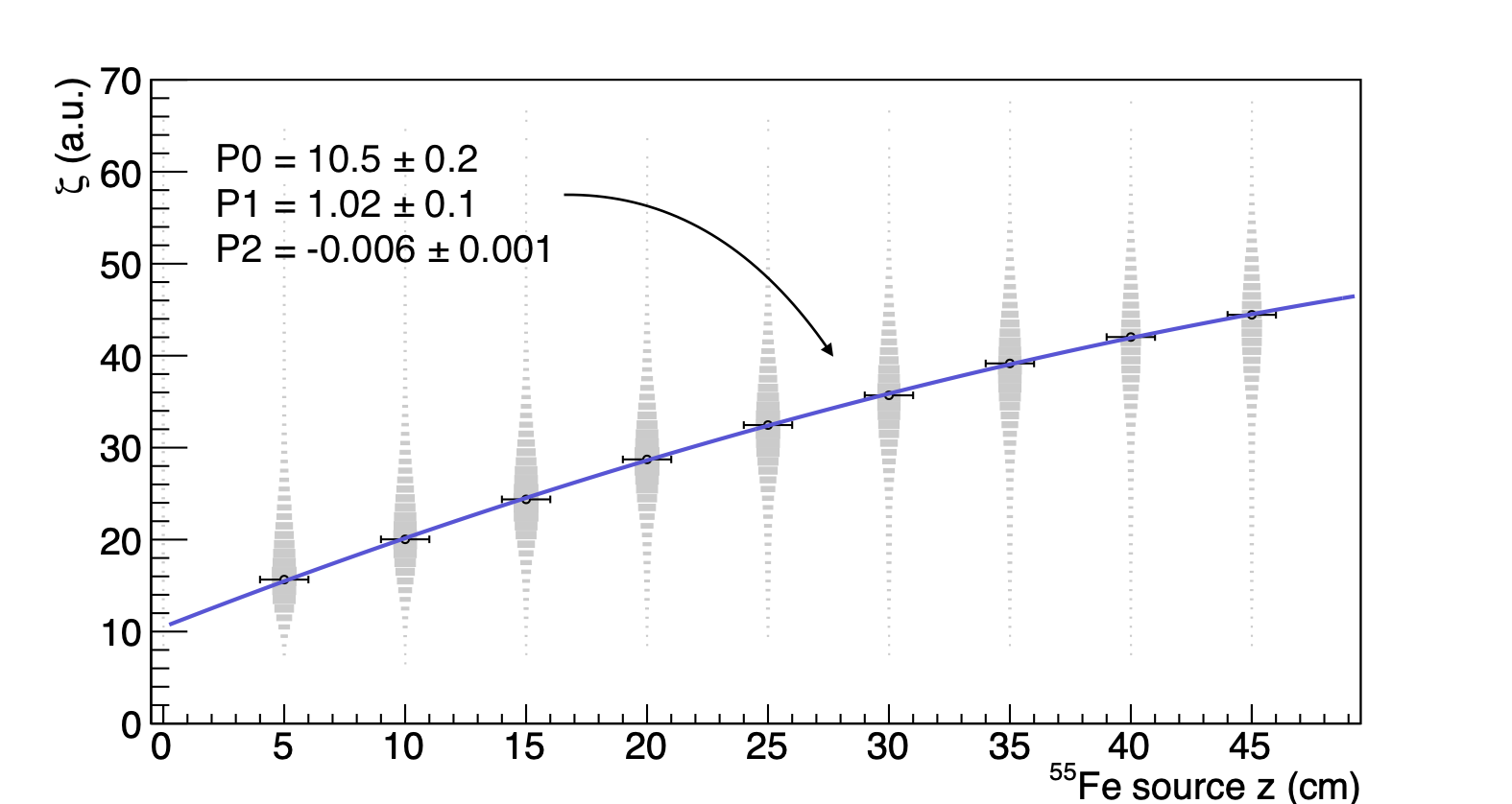
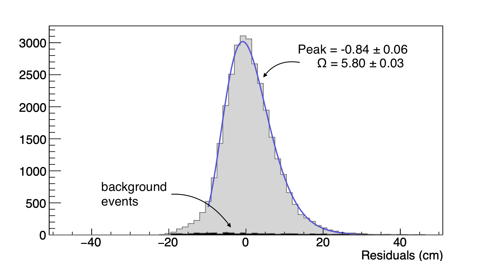
Figure 19: Top: distribution of the values of $\zeta$ (see text) in the runs with the ^55Fe source at different z${}_{\ce{{}^{55}Fe}}$. Bottom: distribution of the $z$-residuals at z${}_{\ce{{}^{55}Fe}}$ = 20 cm with a superimposed fit to the Novosibirsk function.

As can be seen, although there are large tails in all cases, the main part the spots provide values of $\zeta$ increasing as $z$ increases.

Shown on the bottom side of the figure there is the distribution of the $z$ residuals of the clusters reconstructed from the measured $\zeta$ for a z${}_{\ce{{}^{55}Fe}}$ value of 20 cm. The distribution of the residual was fit with a Novosibirsk function bib:novo and from this fit, the value of the parameter $\Omega$ was extracted. The $\Omega$ values obtained for the nine datasets at the various positions are plotted as a function of the nine z${}_{\ce{{}^{55}Fe}}$ in Fig 20.

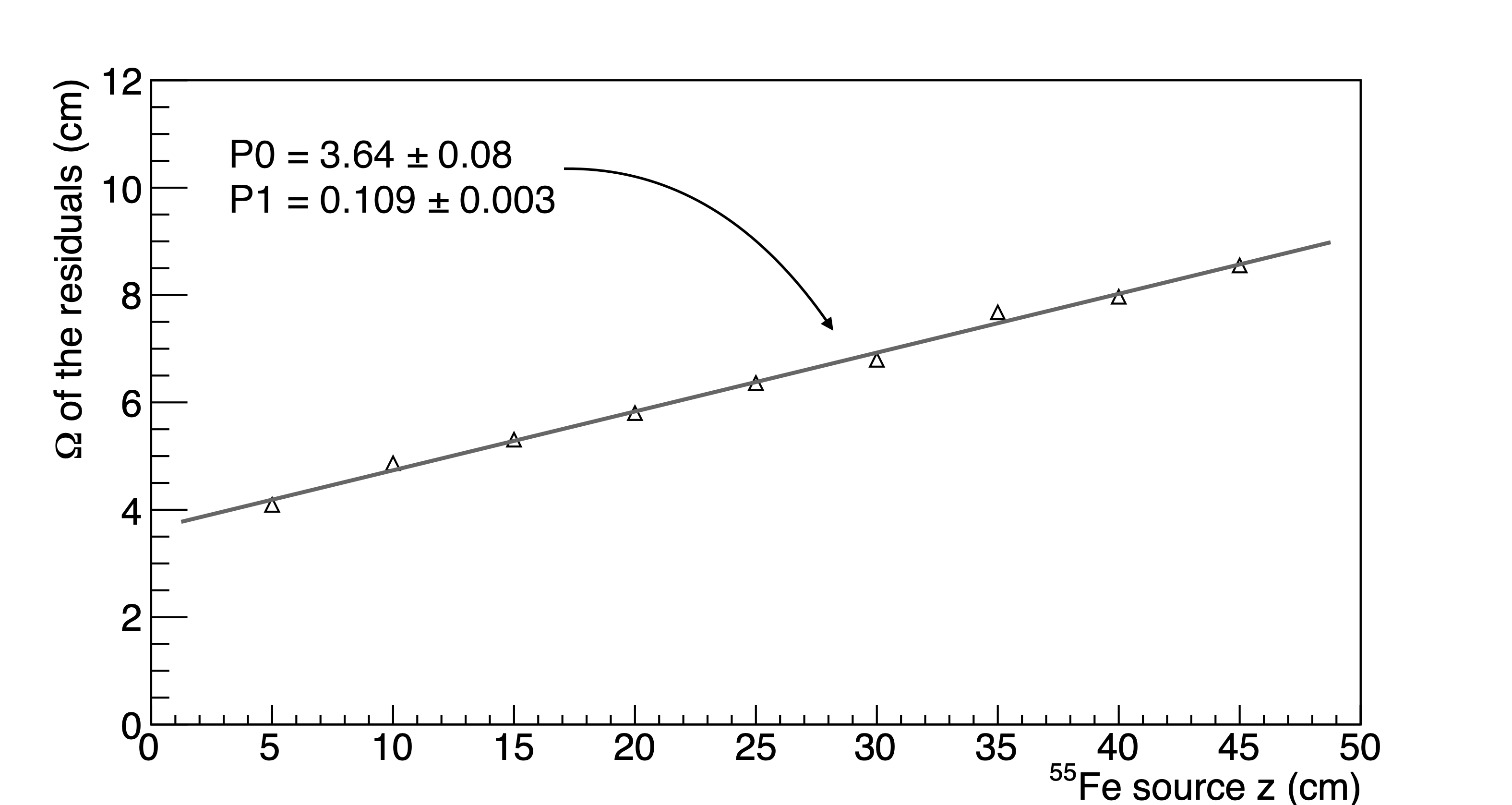
Figure 20: Behaviour of the values of the $\Omega$ evaluated from the Novosibirsk function on the residuals distributions as a function of z${}_{\ce{{}^{55}Fe}}$ with a superimmposed linear fit.

As can be seen, although the absolute uncertainty worsens slightly as the distance of the spots from the GEM increases, this method showed to be able to provide an estimate of $z$ of ^55Fe photons interactions, with an uncertainty of less than $10\text{\,}\mathrm{c}\mathrm{m}$ even for events occurring near the cathode.

6 Study of the absorption length of ^55Fe X-rays

From the above studies the overall LIME performance is found to be excellent to detect low energy electron recoils. We then analyzed the ^55Fe data to measure the average absorption length $\lambda$ of the ^55Fe X-rays. As we have seen, the source mainly emits photons of two different energies (5.9 keV and 6.5 keV). For these two energy values the absorption lengths $\lambda$ in a 60/40 He/CF₄ mixture at atmospheric pressure were estimated (from pressure1 ; pressure2 to be $19.5\text{\,}\mathrm{c}\mathrm{m}$ and $25.6\text{\,}\mathrm{c}\mathrm{m}$, respectively. A variation of the order of 10% of CF₄ fraction reflects in a variation of the $\lambda$ value of about 2.0 cm. In particular, an higher amount of CF₄ results in a lower $\lambda$ value.

A Monte Carlo (MC) technique was then used to evaluate the spatial distribution of the interaction points of a mixture of photons of the two energies (in the proportions reported in Sec.4.4). Being the $z$ coordinate uncertainty relatively large, we used only the $x$ and $y$ coordinates to infer $\lambda$. With this MC we then evaluated the effect of the missing $z$ coordinate information on the measurement of $\lambda$. In this MC we took into account the angular aperture of the X-rays exiting the collimator, estimated to be 20^∘. For each simulated interaction point, the distance $d$ from the source (located above the LIME vessel) was then calculated. From the exponential fit of the $d$ distribution, we obtained a simulated expected value of the effective absorption length $\lambda_{eff}$ = $20.4\text{\,}\mathrm{c}\mathrm{m}$.

In data we then studied the reconstructed $d$ values in runs taken with the ^55Fe source at the nine different distances from the GEM. Some variation of the reconstructed value of $\lambda$ as a function of the range of $y$ studied was found, with large uncertainties in the regions far from the GEM centre where optical distortions are more important. For this reason, our study was carried out eliminating the bands of the top and bottom $6\text{\,}\mathrm{c}\mathrm{m}$ in $y$.

The background distribution in the region of interest was obtained from runs taken without the source. The distribution of $d$ values in this case was found to be substantially flat. The distribution in ^55Fe events was then fitted to an exponential function summed to a constant term fixed to account for the background events.

To study possible systematic effects introduced by the charge transport along the drift field, the reconstructed $\lambda$ was first evaluated at different ^55Fe source positions along the $z$-axis and shown in Fig. 21.

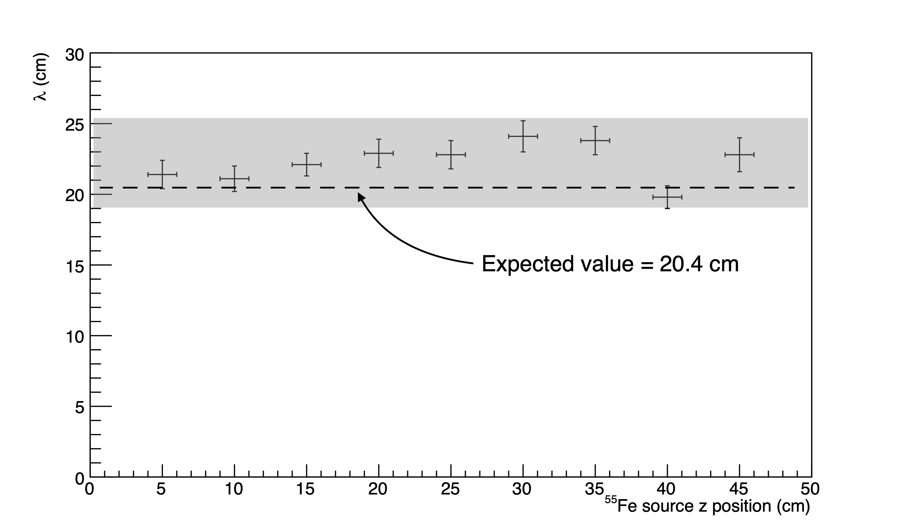
Figure 21: $\lambda$ values resulted from exponential fits to $d$ distribution in data taken with the ^55Fe source at different $z_{\ce{{}^{55}Fe}}$ positions.

Variations of the order of 3.0 cm around the mean value, which is estimated to be $22.4\text{\,}\mathrm{c}\mathrm{m}$, are visible, however no clear systematic trend is present.

Figure 22 shows the distribution of the values of $d$ evaluated at all the $z_{\ce{{}^{55}Fe}}$ with a superimposed fit.

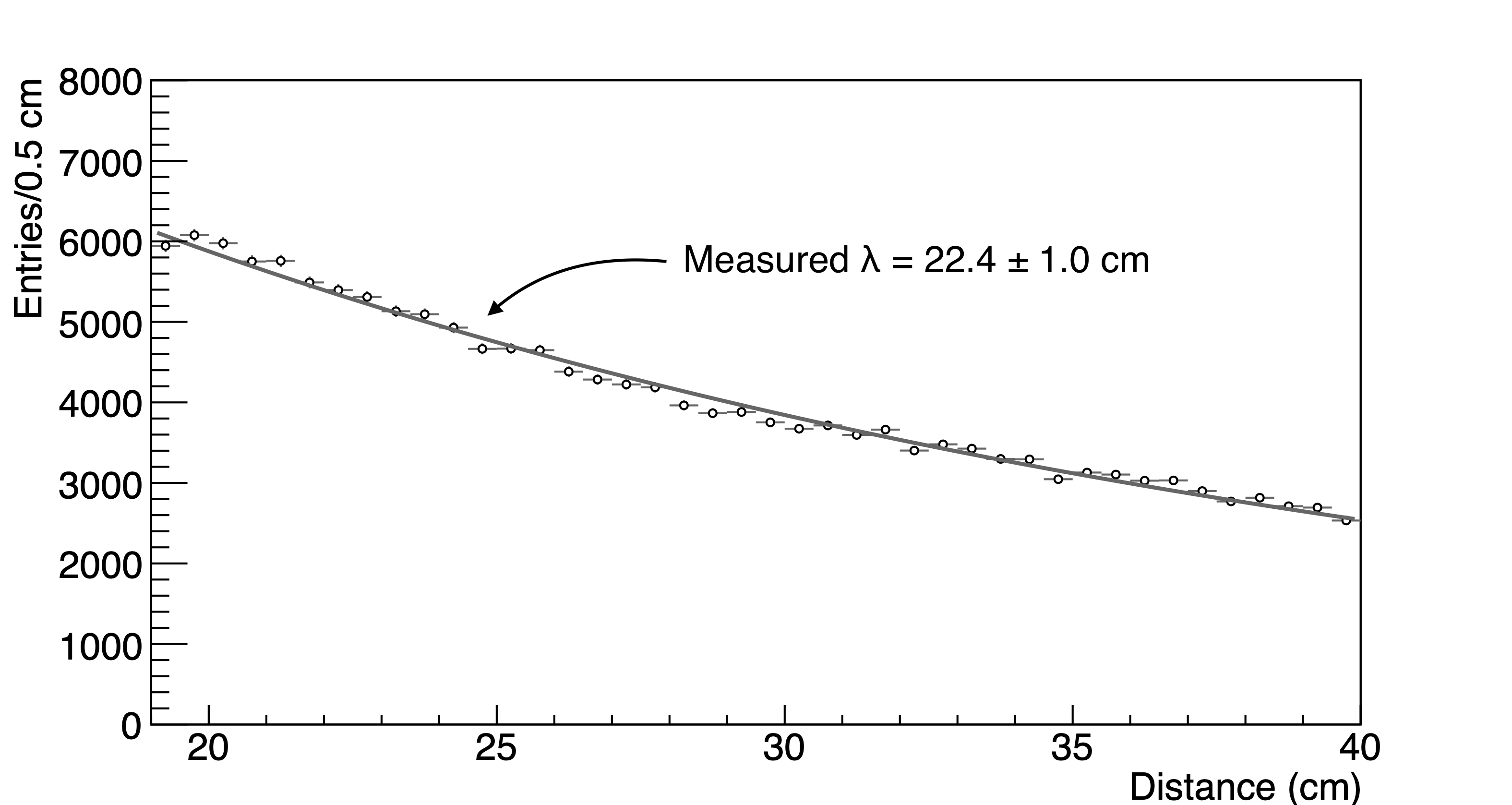
Figure 22: Distribution of $d$ with superimposed exponential fit for all the data at all distance of ^55Fe source from the GEM plane.

This analysis provides a value reasonably in agreement with the expected one, given the statistical fluctuations and possible systematic errors not accounted here.

A more relevant result lies in the fact that in this measurement no systematic effects due to the position of the spots were revealed, either in the $x$–$y$ plane of the image or versus $z_{\ce{{}^{55}Fe}}$. This allows us to conclude that the charge transport and detection efficiency within the sensitive volume of the detector shows good uniformity.

7 Long term stability of detector operation

A DM search is usually requiring long runs of data-taking of months or even years. This imposes the capability to monitor the stability of the performance of the detector over time. We then evaluate the stability of the LIME prototype by maintaining the detector running for two weeks at LNF. Without any direct human intervention, runs of pedestal events and ^55Fe source runs were automatically collected. In two occasions, data were not properly saved because of an issue with the internal network of the laboratory.

The laboratory is equipped with a heating system to keep the temperature under control. Therefore in this period the room temperature was found to be quite stable with an average value of 298.7 $\pm$ 0.3 K. In the same period the atmospheric pressure showed visible variations with an important oscillation of about $15\text{\,}\mathrm{m}\mathrm{b}\mathrm{a}\mathrm{r}$ in the latest period of the test as it is shown on the bottom in Fig. 23.

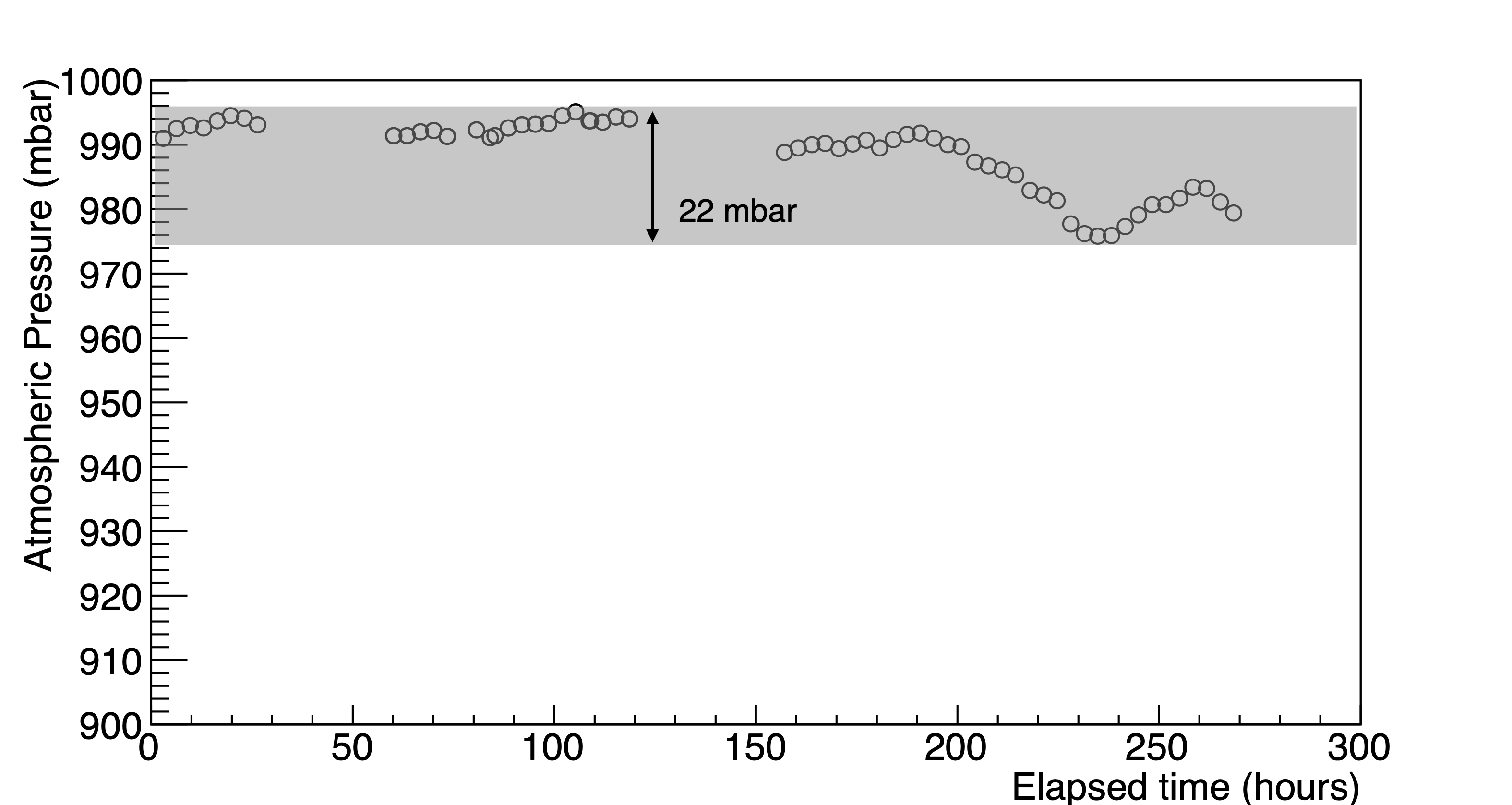
Figure 23: Atmospheric pressure recorded during the runs acquired for the test on the LIME’s response stability.

The average number of photons in the spots of ^55Fe X-ray interactions was evaluated and its behavior (normalised to the initial value) is shown on the top in Fig. 24.

The detector light yield shows an almost constant increase during the whole data-taking period. This behavior can be directly correlated with the variation of the gas pressure as shown on the bottom of Fig. 24.

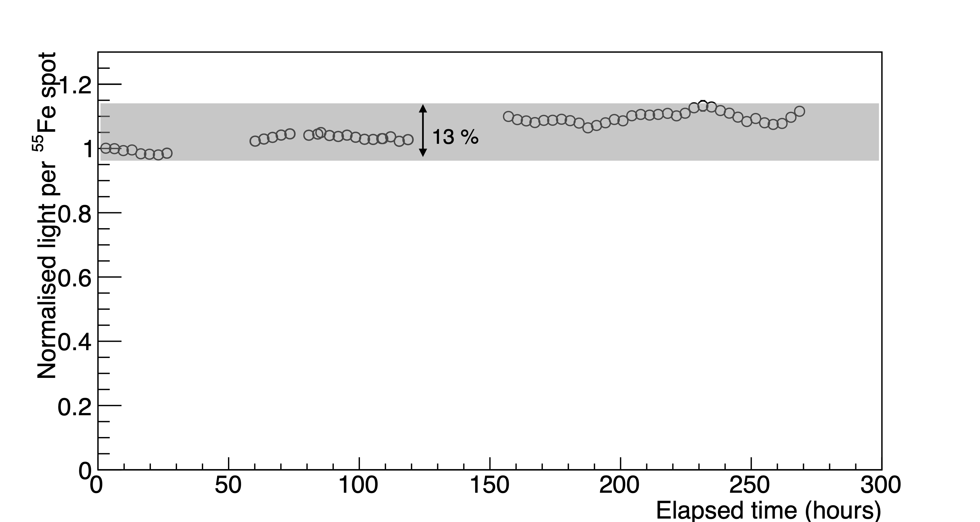
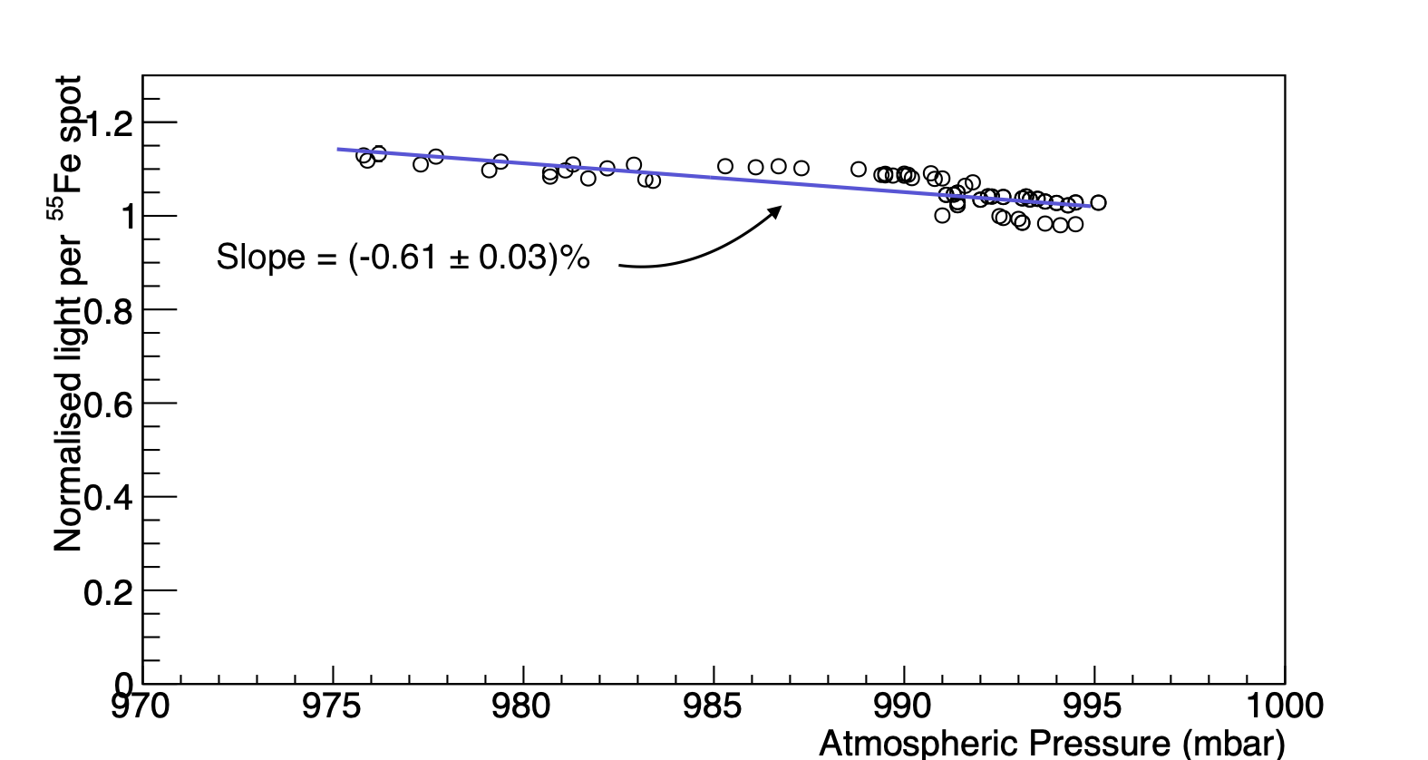
Figure 24: Behavior of the number of photons as a function of elapsed time normalised to the initial value (top) and as a function of the atmospheric pressure (bottom) with a superimposed linear fit.

From the result of the superimposed linear fit, we evaluated a light yield decrease of about 0.6% per millibar due to the expected decrease of the gas gain with the increasing of the gas density bib:blum .

8 Background evaluation at LNF

The data taken with the LIME prototype at LNF in absence of any artificial source were analyzed. A number of interactions of particles in the active volume were detected. The origin of these particle can be ascribed to various sources, primarily the decays of radioactive elements present in the materials of the detector itself and of the surrounding environment and cosmic rays. Those interactions are to be considered as a background in searches for ultra-rare events as the interaction of a DM particle in the detector. A first assessment of this background is therefore necessary to understand how to improve in future the radiopurity of the detector itself. Shielding against cosmic rays can be achieved by operating the detector in an underground location (as INFN LNGS) while the effect of the radioactivity of the surrounding environment can be largely mitigated by using high radiopurity passive materials (as water or copper) around the active volume of the detector.

The analysis of the images reveals the presence of several interactions that the reconstruction algorithm is able to identify with a very good efficiency. Due to the fact that LIME was not built with radiopure materials and given the overground location of the data-taking, crowded images are usually acquired and analyzed. Sometimes, because of the piling-up of two or more tracks in the image, the reconstruction can lead to an inaccurate estimate of the number of tracks. Because the iterative procedure of the step (iii) of the reconstruction, described in Sec. 4.1, when a long cluster is reconstructed all the pixels belonging to it are removed. This implies that in the next iteration the pixels in the overlap region with another track are no more available and the other overlapping track is typically split in two pieces. This results in a number of reconstructed long clusters systematically higher than the true one.

In Fig. 25 (top) the distribution of the number of reconstructed super-cluster per image in a sample of $\approx 2000$ images is shown. Each image corresponds to a live-time (i.e. the total exposure time of the camera) of $50\text{\,}\mathrm{m}\mathrm{s}$ and these images were acquired in a period of about 10 minutes. The requirement $\text{\,}\mathrm{I}_{SC}$$>$400\text{\,}\mathrm{p}\mathrm{h}\mathrm{o}\mathrm{t}\mathrm{o}\mathrm{n}\mathrm{s}$$ is applied on the minimal energy of the cluster, in order to remove the contribution of the fake clusters, as shown in Fig. 10 (top), which corresponds to a threshold of $E\gtrsim$300\text{\,}\mathrm{e}\mathrm{V}$$. This corresponds to an average rate of detected interaction of $r\approx$250\text{\,}\mathrm{H}\mathrm{z}$$. Figure 25 (bottom) shows the distribution of the energy sum for all the clusters satisfying the above minimum energy threshold in one image, defined as $S_{\mathrm{thr}}$. The average $S_{\mathrm{thr}}$ per unit time is $\approx$6.3\text{\,}\mathrm{M}\mathrm{e}\mathrm{V}\mathrm{/}\mathrm{s}$$.

During the data taking a 3x3 inches NaI crystal scintillator detector (Ortec 905-4) was used to measure the environmental radioactivity in the LNF location of LIME. The lowest threshold to operate this NaI detector was $85\text{\,}\mathrm{k}\mathrm{e}\mathrm{V}$. A rate of $350\text{\,}\mathrm{H}\mathrm{z}$ of energy deposits was measured. By scaling this NaI rate to the mass of the LIME active volume a rate of $11\text{\,}\mathrm{H}\mathrm{z}$ is predicted. This can be compared with the average rate of $\approx$20\text{\,}\mathrm{H}\mathrm{z}$$ measured by counting the number of reconstructed cluster with $E>$85\text{\,}\mathrm{k}\mathrm{e}\mathrm{V}$$ in LIME whose distribution is shown in Fig. 25 (middle). For this comparison we selected only the clusters in a central region of the active volume where the signal to noise ratio is larger. This corresponds to a geometrical acceptance of about 50%. This demonstrated that at the LNF location only part of the contribution to background is due to the external radioactivity.

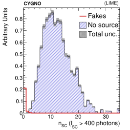
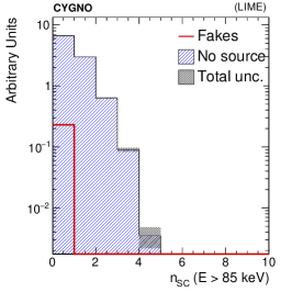
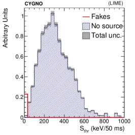
Figure 25: Top: number of clusters reconstructed in each image with a minimal threshold on the light yield to remove fake clusters, $\text{\,}\mathrm{I}_{SC}$$>$400\text{\,}\mathrm{p}\mathrm{h}\mathrm{o}\mathrm{t}\mathrm{o}\mathrm{n}\mathrm{s}$$ (corresponding to an energy $E\gtrsim$300\text{\,}\mathrm{e}\mathrm{V}$$). Middle: number of clusters with energy $E>$85\text{\,}\mathrm{k}\mathrm{e}\mathrm{V}$$ reconstructed in each image. Bottom: distribution of $S_{\mathrm{thr}}$, sum of the energy for all the reconstructed clusters in one image with energy $E\gtrsim$300\text{\,}\mathrm{e}\mathrm{V}$$. The filled histogram represents data without the source, while the red hollow histograms represents the estimated contribution from fake clusters. All the images have been acquired with an exposure of $50\text{\,}\mathrm{m}\mathrm{s}$.

The overground location of the LIME prototype implies that a significant flux of cosmic rays traverses the active volume, releasing energy with their typical energy pattern of straight lines. This allows to define a cosmic rays sample with excellent purity by applying a simple selection on basic cluster shapes. The track length can be estimated as the major axis of the cluster and compared with the length of a curved path interpolating the cluster shape. By requiring the ratio of the these two variable to be larger than 0.9, straight tracks are selected against curly tracks due to natural radioactivity. Further requirements are the track length being larger than $10\text{\,}\mathrm{c}\mathrm{m}$ and the ratio between the $\sigma_{\mathrm{T}}$ and the length lower than 0.1 in order to avoid tracks with small branches due to mis-reconstructed overlapping clusters. The ratio between the energy $E$ associated to the cosmic ray cluster and its length can be described in terms of the specific ionization of a minimum ionizing particle. Using the standard cosmic ray flux at sea level of $\approx$70\text{\,}\mathrm{H}\mathrm{z}\,\mathrm{m}^{-2}\,\mathrm{s}\mathrm{r}^{-1}$$ Workman:2022ynf we predict a maximum rate of interaction in the active volume of $\approx$ $24\text{\,}\mathrm{H}\mathrm{z}$ to be compared with a measured rate of $\approx$ $15\text{\,}\mathrm{H}\mathrm{z}$.

The track length of the cosmic ray clusters reconstructed by the camera images is in fact the $x$–$y$ projection of the actual trajectory length in 3D of the cosmic ray particles. Therefore a MC simulation of the interaction of cosmic rays with momenta in the range $[1-100]\,{\rm GeV}$ in the LIME active volume taking into account their angular distribution has been carried out. A comparison of the specific ionization evaluated on the data and MC for the cosmic rays is reported in Fig. 26 showing a good agreement.

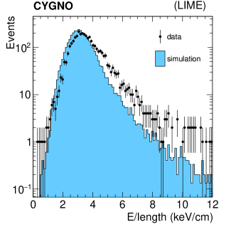
Figure 26: Distributions of energy divide by the total length, of clusters identified as cosmic rays. Black points represent data, filled histogram represents a Monte Carlo simulated sample.

9 Conclusion and perspective

The search for DM particles requires a vast experimental program with different strategies being put forward. A sensitivity to DM masses below 10 GeV might be useful to test alternative model to WIMPs. Experimental tools to infer the DM direction would represent a powerful ingredient to reject background events in the context of future DM searches. The Cygno project aim at demonstrating that a gaseous TPC with GEM amplification and optical readout, operating at atmospheric pressure with a He/CF₄ mixture might represent a viable candidate for a future generation of DM direct searches with directional sensitivity.

In this paper we have fully described the calibration and reconstruction techniques developed for a 50 liters prototype - named LIME - with a mass of 87 g in its active volume that represents 1/18 of a 1 m³ detector. LIME was operated in an overground location at INFN LNF with no shielding against environmental radioactivity.

With LIME we studied the interaction of X-ray in the energy range from few keV to tens of keV with artificial radioactive source. The use of a scientific CMOS camera with single photon sensitivity allowed to identify spots of light originated by the electron recoil energy deposit in the active gas volume. A very good linearity over two decades of energy was demonstrated with a $\approx 10$% energy resolution thanks a regression algorithm exploiting at best all the topological information of the energy deposits. A position reconstruction was possible in the plane transverse to the ionization electron drift thanks to the high granularity of the CMOS readout and with an algorithm based on the ionization electrons diffusion to measure the longitudinal coordinate.

Moreover the absorption length of ^55Fe X-ray was measured and found compatible with the expectation demonstrating a good control of the uniformity and efficiency of the detector. Also during a more than a week long data-taking a remarkable stability of the detector was achieved.

Cosmic rays were also easily identified and their specific ionization results very compatible with the usual prediction in gas.

An analysis of the events detected in absence of any artificial source showed that the detected photon interaction rate (about 20 Hz) can be partly understood in terms of the ambient radioactivity. However given the long integration time (50 ms) of the sCMOS camera the pile-up of interaction in the active volume can lead to an overestimate of the number of interaction. This implies the necessity to operate LIME in a shielded environment as INFN LNGS with a tenfold reduction of the external background. This will reduce to a negligible levle the pile-up in images and will allow an assessment of the level of radiopurity of the materials used for LIME. This measurements will be the basis for the design of a future Cygno DM detector.

In future a direct evaluation of the capability of LIME to identify nuclear recoils induced by neutron will be performed with dedicated calibration data-taking. Given the performance of LIME in reconstructing in details the topology of the energy deposit a very good nuclear recoil identification down to few keV is foreseen coronello . This will represent the fundamental element of a competitive DM detector.

- (1) S.E. Vahsen, et al., (2020)
- (2) F. Sauli, Nucl. Instrum. Meth. A 386, 531 (1997). DOI 10.1016/S0168-9002(96)01172-2
- (3) F.D. Amaro, E. Baracchini, L. Benussi, S. Bianco, C. Capoccia, M. Caponero, D.S. Cardoso, G. Cavoto, A. Cortez, I.A. Costa, R.J.d.C. Roque, E. Dané, G. Dho, F. Di Giambattista, E. Di Marco, G. Grilli di Cortona, G. D’Imperio, F. Iacoangeli, H.P. Lima Júnior, G.S. Pinheiro Lopes, A.d.S. Lopes Júnior, G. Maccarrone, R.D.P. Mano, M. Marafini, R.R. Marcelo Gregorio, D.J.G. Marques, G. Mazzitelli, A.G. McLean, A. Messina, C.M. Bernardes Monteiro, R.A. Nobrega, I.F. Pains, E. Paoletti, L. Passamonti, S. Pelosi, F. Petrucci, S. Piacentini, D. Piccolo, D. Pierluigi, D. Pinci, A. Prajapati, F. Renga, F. Rosatelli, A. Russo, J.M.F. dos Santos, G. Saviano, N.J.C. Spooner, R. Tesauro, S. Tomassini, S. Torelli, Instruments 6(1) (2022). DOI 10.3390/instruments6010006. URL https://www.mdpi.com/2410-390X/6/1/6
- (4) G. Bertone, D. Hooper, J. Silk, Physics reports 405(5-6), 279 (2005)
- (5) G. Bertone, D. Hooper, Rev. Mod. Phys. 90, 045002 (2018). DOI 10.1103/RevModPhys.90.045002. URL https://link.aps.org/doi/10.1103/RevModPhys.90.045002
- (6) E. Aprile, et al., Phys. Rev. Lett. 121(11), 111302 (2018). DOI 10.1103/PhysRevLett.121.111302
- (7) J. Aalbers, D.S. Akerib, C.W. Akerlof, A.K.A. Musalhi, F. Alder, A. Alqahtani, S.K. Alsum, C.S. Amarasinghe, A. Ames, T.J. Anderson, N. Angelides, H.M. Araújo, J.E. Armstrong, M. Arthurs, S. Azadi, A.J. Bailey, A. Baker, J. Balajthy, S. Balashov, J. Bang, J.W. Bargemann, M.J. Barry, J. Barthel, D. Bauer, A. Baxter, K. Beattie, J. Belle, P. Beltrame, J. Bensinger, T. Benson, E.P. Bernard, A. Bhatti, A. Biekert, T.P. Biesiadzinski, H.J. Birch, B. Birrittella, G.M. Blockinger, K.E. Boast, B. Boxer, R. Bramante, C.A.J. Brew, P. Brás, J.H. Buckley, V.V. Bugaev, S. Burdin, J.K. Busenitz, M. Buuck, R. Cabrita, C. Carels, D.L. Carlsmith, B. Carlson, M.C. Carmona-Benitez, M. Cascella, C. Chan, A. Chawla, H. Chen, J.J. Cherwinka, N.I. Chott, A. Cole, J. Coleman, M.V. Converse, A. Cottle, G. Cox, W.W. Craddock, O. Creaner, D. Curran, A. Currie, J.E. Cutter, C.E. Dahl, A. David, J. Davis, T.J.R. Davison, J. Delgaudio, S. Dey, L. de Viveiros, A. Dobi, J.E.Y. Dobson, E. Druszkiewicz, A. Dushkin, T.K. Edberg, W.R. Edwards, M.M. Elnimr, W.T. Emmet, S.R. Eriksen, C.H. Faham, A. Fan, S. Fayer, N.M. Fearon, S. Fiorucci, H. Flaecher, P. Ford, V.B. Francis, E.D. Fraser, T. Fruth, R.J. Gaitskell, N.J. Gantos, D. Garcia, A. Geffre, V.M. Gehman, J. Genovesi, C. Ghag, R. Gibbons, E. Gibson, M.G.D. Gilchriese, S. Gokhale, B. Gomber, J. Green, A. Greenall, S. Greenwood, M.G.D. van der Grinten, C.B. Gwilliam, C.R. Hall, S. Hans, K. Hanzel, A. Harrison, E. Hartigan-O’Connor, S.J. Haselschwardt, S.A. Hertel, G. Heuermann, C. Hjemfelt, M.D. Hoff, E. Holtom, J.Y.K. Hor, M. Horn, D.Q. Huang, D. Hunt, C.M. Ignarra, R.G. Jacobsen, O. Jahangir, R.S. James, S.N. Jeffery, W. Ji, J. Johnson, A.C. Kaboth, A.C. Kamaha, K. Kamdin, V. Kasey, K. Kazkaz, J. Keefner, D. Khaitan, M. Khaleeq, A. Khazov, I. Khurana, Y.D. Kim, C.D. Kocher, D. Kodroff, L. Korley, E.V. Korolkova, J. Kras, H. Kraus, S. Kravitz, H.J. Krebs, L. Kreczko, B. Krikler, V.A. Kudryavtsev, S. Kyre, B. Landerud, E.A. Leason, C. Lee, J. Lee, D.S. Leonard, R. Leonard, K.T. Lesko, C. Levy, J. Li, F.T. Liao, J. Liao, J. Lin, A. Lindote, R. Linehan, W.H. Lippincott, R. Liu, X. Liu, Y. Liu, C. Loniewski, M.I. Lopes, E.L. Asamar, B.L. Paredes, W. Lorenzon, D. Lucero, S. Luitz, J.M. Lyle, P.A. Majewski, J. Makkinje, D.C. Malling, A. Manalaysay, L. Manenti, R.L. Mannino, N. Marangou, M.F. Marzioni, C. Maupin, M.E. McCarthy, C.T. McConnell, D.N. McKinsey, J. McLaughlin, Y. Meng, J. Migneault, E.H. Miller, E. Mizrachi, J.A. Mock, A. Monte, M.E. Monzani, J.A. Morad, J.D.M. Mendoza, E. Morrison, B.J. Mount, M. Murdy, A.S.J. Murphy, D. Naim, A. Naylor, C. Nedlik, C. Nehrkorn, H.N. Nelson, F. Neves, A. Nguyen, J.A. Nikoleyczik, A. Nilima, J. O’Dell, F.G. O’Neill, K. O’Sullivan, I. Olcina, M.A. Olevitch, K.C. Oliver-Mallory, J. Orpwood, D. Pagenkopf, S. Pal, K.J. Palladino, J. Palmer, M. Pangilinan, N. Parveen, S.J. Patton, E.K. Pease, B. Penning, C. Pereira, G. Pereira, E. Perry, T. Pershing, I.B. Peterson, A. Piepke, J. Podczerwinski, D. Porzio, S. Powell, R.M. Preece, K. Pushkin, Y. Qie, B.N. Ratcliff, J. Reichenbacher, L. Reichhart, C.A. Rhyne, A. Richards, Q. Riffard, G.R.C. Rischbieter, J.P. Rodrigues, A. Rodriguez, H.J. Rose, R. Rosero, P. Rossiter, T. Rushton, G. Rutherford, D. Rynders, J.S. Saba, D. Santone, A.B.M.R. Sazzad, R.W. Schnee, P.R. Scovell, D. Seymour, S. Shaw, T. Shutt, J.J. Silk, C. Silva, G. Sinev, K. Skarpaas, W. Skulski, R. Smith, M. Solmaz, V.N. Solovov, P. Sorensen, J. Soria, I. Stancu, M.R. Stark, A. Stevens, T.M. Stiegler, K. Stifter, R. Studley, B. Suerfu, T.J. Sumner, P. Sutcliffe, N. Swanson, M. Szydagis, M. Tan, D.J. Taylor, R. Taylor, W.C. Taylor, D.J. Temples, B.P. Tennyson, P.A. Terman, K.J. Thomas, D.R. Tiedt, M. Timalsina, W.H. To, A. Tomás, Z. Tong, D.R. Tovey, J. Tranter, M. Trask, M. Tripathi, D.R. Tronstad, C.E. Tull, W. Turner, L. Tvrznikova, U. Utku, J. Va’vra, A. Vacheret, A.C. Vaitkus, J.R. Verbus, E. Voirin, W.L. Waldron, A. Wang, B. Wang, J.J. Wang, W. Wang, Y. Wang, J.R. Watson, R.C. Webb, A. White, D.T. White, J.T. White, R.G. White, T.J. Whitis, M. Williams, W.J. Wisniewski, M.S. Witherell, F.L.H. Wolfs, J.D. Wolfs, S. Woodford, D. Woodward, S.D. Worm, C.J. Wright, Q. Xia, X. Xiang, Q. Xiao, J. Xu, M. Yeh, J. Yin, I. Young, P. Zarzhitsky, A. Zuckerman, E.A. Zweig. First dark matter search results from the lux-zeplin (lz) experiment (2022)
- (8) R. Bernabei, et al., Eur. Phys. J. C 73, 2648 (2013). DOI 10.1140/epjc/s10052-013-2648-7
- (9) D.S. Akerib, et al., Phys. Rev. Lett. 118(2), 021303 (2017). DOI 10.1103/PhysRevLett.118.021303
- (10) X. Cui, et al., Phys. Rev. Lett. 119(18), 181302 (2017). DOI 10.1103/PhysRevLett.119.181302
- (11) F. Mayet, A. Green, J. Battat, J. Billard, N. Bozorgnia, G. Gelmini, P. Gondolo, B. Kavanagh, S. Lee, D. Loomba, J. Monroe, B. Morgan, C. O’Hare, A. Peter, N. Phan, S. Vahsen, Physics Reports 627, 1 (2016). DOI https://doi.org/10.1016/j.physrep.2016.02.007. URL https://www.sciencedirect.com/science/article/pii/S0370157316001022. A review of the discovery reach of directional Dark Matter detection
- (12) J. Battat, et al., Phys. Dark Univ. 9-10, 1 (2015). DOI 10.1016/j.dark.2015.06.001
- (13) J. Battat, et al., Phys. Rept. 662, 1 (2016). DOI 10.1016/j.physrep.2016.10.001
- (14) J. Battat, et al., Astropart. Phys. 91, 65 (2017). DOI 10.1016/j.astropartphys.2017.03.007
- (15) J.B. Battat, C. Deaconu, G. Druitt, R. Eggleston, P. Fisher, P. Giampa, V. Gregoric, S. Henderson, I. Jaegle, J. Lawhorn, J.P. Lopez, J. Monroe, K.A. Recine, A. Strandberg, H. Tomita, S. Vahsen, H. Wellenstein, Nuclear Instruments and Methods in Physics Research Section A: Accelerators, Spectrometers, Detectors and Associated Equipment 755, 6 (2014). DOI https://doi.org/10.1016/j.nima.2014.04.010. URL http://www.sciencedirect.com/science/article/pii/S016890021400388X
- (16) E. Daw, et al., JINST 9, P07021 (2014). DOI 10.1088/1748-0221/9/07/P07021
- (17) J. Battat, et al., Nucl. Instrum. Meth. A 794, 33 (2015). DOI 10.1016/j.nima.2015.04.070
- (18) N. Phan, E. Lee, D. Loomba, JINST 15(05), P05012 (2020). DOI 10.1088/1748-0221/15/05/P05012
- (19) E. Baracchini, G. Cavoto, G. Mazzitelli, F. Murtas, F. Renga, S. Tomassini, Journal of Instrumentation 13(04), P04022 (2018). DOI 10.1088/1748-0221/13/04/p04022. URL https://doi.org/10.1088%2F1748-0221%2F13%2F04%2Fp04022
- (20) T. Ikeda, K. Miuchi, T. Hashimoto, H. Ishiura, T. Nakamura, T. Shimada, K. Nakamura, J. Phys. Conf. Ser. 1468(1), 012042 (2020). DOI 10.1088/1742-6596/1468/1/012042
- (21) Q. Riffard, et al., JINST 11(08), P08011 (2016). DOI 10.1088/1748-0221/11/08/P08011
- (22) N. Sauzet, D. Santos, O. Guillaudin, G. Bosson, J. Bouvier, T. Descombes, M. Marton, J. Muraz, J. Phys. Conf. Ser. 1498(1), 012044 (2020). DOI 10.1088/1742-6596/1498/1/012044
- (23) T. Hashimoto, K. Miuchi, K. Nakamura, R. Yakabe, T. Ikeda, R. Taishaku, M. Nakazawa, H. Ishiura, A. Ochi, Y. Takeuchi, AIP Conf. Proc. 1921(1), 070001 (2018). DOI 10.1063/1.5019004
- (24) J. Battat, J. Brack, E. Daw, A. Dorofeev, A. Ezeribe, J.L. Gauvreau, M. Gold, J. Harton, J. Landers, E. Law, E. Lee, D. Loomba, A. Lumnah, J. Matthews, E. Miller, A. Monte, F. Mouton, A. Murphy, S. Paling, N. Phan, M. Robinson, S. Sadler, A. Scarff, F. Schuckman II, D. Snowden-Ifft, N. Spooner, S. Telfer, S. Vahsen, D. Walker, D. Warner, L. Yuriev, Physics of the Dark Universe 9-10, 1 (2015). DOI https://doi.org/10.1016/j.dark.2015.06.001. URL http://www.sciencedirect.com/science/article/pii/S2212686415000084
- (25) G. Alner, H. Araujo, A. Bewick, S. Burgos, M. Carson, J. Davies, E. Daw, J. Dawson, J. Forbes, T. Gamble, M. Garcia, C. Ghag, M. Gold, S. Hollen, R. Hollingworth, A. Howard, J. Kirkpatrick, V. Kudryavtsev, T. Lawson, V. Lebedenko, J. Lewin, P. Lightfoot, I. Liubarsky, D. Loomba, R. Lüscher, J. McMillan, B. Morgan, D. Muna, A. Murphy, G. Nicklin, S. Paling, A. Petkov, S. Plank, R. Preece, J. Quenby, M. Robinson, N. Sanghi, N. Smith, P. Smith, D. Snowden-Ifft, N. Spooner, T. Sumner, D. Tovey, J. Turk, E. Tziaferi, R. Walker, Nuclear Instruments and Methods in Physics Research Section A: Accelerators, Spectrometers, Detectors and Associated Equipment 555(1), 173 (2005). DOI https://doi.org/10.1016/j.nima.2005.09.011. URL http://www.sciencedirect.com/science/article/pii/S0168900205018139
- (26) S. Vahsen, K. Oliver-Mallory, M. Lopez-Thibodeaux, J. Kadyk, M. Garcia-Sciveres, Nucl. Instrum. Meth. A 738, 111 (2014). DOI 10.1016/j.nima.2013.10.029
- (27) K. Petraki, R.R. Volkas, International Journal of Modern Physics A 28(19), 1330028 (2013)
- (28) K.M. Zurek, Physics Reports 537(3), 91 (2014). DOI 10.1016/j.physrep.2013.12.001. URL https://doi.org/10.1016%2Fj.physrep.2013.12.001
- (29) Y. Hochberg, E. Kuflik, H. Murayama, T. Volansky, J.G. Wacker, Phys. Rev. Lett. 115, 021301 (2015). DOI 10.1103/PhysRevLett.115.021301. URL https://link.aps.org/doi/10.1103/PhysRevLett.115.021301
- (30) M. Fraga, F. Fraga, S. Fetal, L. Margato, R. Marques, A. Policarpo, Nuclear Instruments and Methods in Physics Research Section A: Accelerators, Spectrometers, Detectors and Associated Equipment 504(1), 88 (2003). DOI https://doi.org/10.1016/S0168-9002(03)00758-7. URL http://www.sciencedirect.com/science/article/pii/S0168900203007587. Proceedings of the 3rd International Conference on New Developments in Photodetection
- (31) M.M.F.R. Fraga, F.A.F. Fraga, S.T.G. Fetal, L.M.S. Margato, R. Ferreira-Marques, A.J.P.L. Policarpo, Nucl. Instrum. Meth. A504, 88 (2003). DOI 10.1016/S0168-9002(03)00758-7
- (32) J.B.R. Battat, et al., Nucl. Instrum. Meth. A 755, 6 (2014). DOI 10.1016/j.nima.2014.04.010
- (33) S. Ahlen, et al., Phys. Lett. B 695, 124 (2011). DOI 10.1016/j.physletb.2010.11.041
- (34) D. Dujmic, H. Tomita, M. Lewandowska, S. Ahlen, P. Fisher, S. Henderson, A. Kaboth, G. Kohse, R. Lanza, J. Monroe, A. Roccaro, G. Sciolla, N. Skvorodnev, R. Vanderspek, H. Wellenstein, R. Yamamoto, Nuclear Instruments and Methods in Physics Research Section A: Accelerators, Spectrometers, Detectors and Associated Equipment 584(2), 327 (2008). DOI https://doi.org/10.1016/j.nima.2007.10.037. URL https://www.sciencedirect.com/science/article/pii/S016890020702222X
- (35) C. Deaconu, M. Leyton, R. Corliss, G. Druitt, R. Eggleston, N. Guerrero, S. Henderson, J. Lopez, J. Monroe, P. Fisher, Phys. Rev. D 95, 122002 (2017). DOI 10.1103/PhysRevD.95.122002. URL https://link.aps.org/doi/10.1103/PhysRevD.95.122002
- (36) M. Marafini, V. Patera, D. Pinci, A. Sarti, A. Sciubba, E. Spiriti, Nucl. Instrum. Meth. A845, 285 (2017). DOI 10.1016/j.nima.2016.04.014
- (37) M. Marafini, V. Patera, D. Pinci, A. Sarti, A. Sciubba, E. Spiriti, JINST 10(12), P12010 (2015). DOI 10.1088/1748-0221/10/12/P12010
- (38) M. Marafini, V. Patera, D. Pinci, A. Sarti, A. Sciubba, N.M. Torchia, IEEE Transactions on Nuclear Science 65, 604 (2018). DOI 10.1109/TNS.2017.2778503
- (39) M. Marafini, V. Patera, D. Pinci, A. Sarti, A. Sciubba, E. Spiriti, Nuclear Instruments and Methods in Physics Research Section A: Accelerators, Spectrometers, Detectors and Associated Equipment 824, 562 (2016). DOI https://doi.org/10.1016/j.nima.2015.11.058. URL http://www.sciencedirect.com/science/article/pii/S0168900215014230. Frontier Detectors for Frontier Physics: Proceedings of the 13th Pisa Meeting on Advanced Detectors
- (40) V.C. Antochi, E. Baracchini, G. Cavoto, E.D. Marco, M. Marafini, G. Mazzitelli, D. Pinci, F. Renga, S. Tomassini, C. Voena, JINST 13(05), P05001 (2018). DOI 10.1088/1748-0221/13/05/P05001
- (41) I. Abritta Costa, et al., J. Phys. Conf. Ser. 1498, 012016 (2020). DOI 10.1088/1742-6596/1498/1/012016
- (42) I.A. Costa, E. Baracchini, F. Bellini, L. Benussi, S. Bianco, M. Caponero, G. Cavoto, G. D’Imperio, E.D. Marco, G. Maccarrone, M. Marafini, G. Mazzitelli, A. Messina, F. Petrucci, D. Piccolo, D. Pinci, F. Renga, F. Rosatelli, G. Saviano, S. Tomassini, Journal of Instrumentation 14(07), P07011 (2019). DOI 10.1088/1748-0221/14/07/p07011. URL https://doi.org/10.1088%2F1748-0221%2F14%2F07%2Fp07011
- (43) I.A. Costa, E. Baracchini, F. Bellini, L. Benussi, S. Bianco, M. Caponero, G. Cavoto, G. D’Imperio, E.D. Marco, G. Maccarrone, M. Marafini, G. Mazzitelli, A. Messina, F. Petrucci, D. Piccolo, D. Pinci, F. Renga, F. Rosatelli, G. Saviano, S. Tomassini, Journal of Instrumentation 14(07), P07011 (2019). DOI 10.1088/1748-0221/14/07/p07011
- (44) E. Baracchini, et al., JINST 15(10), P10001 (2020). DOI 10.1088/1748-0221/15/10/P10001
- (45) E. Baracchini, R. Bedogni, F. Bellini, L. Benussi, S. Bianco, L. Bignell, M. Caponero, G. Cavoto, E.D. Marco, C. Eldridge, A. Ezeribe, R. Gargana, T. Gamble, R. Gregorio, G. Lane, D. Loomba, W. Lynch, G. Maccarrone, M. Marafini, G. Mazzitelli, A. Messina, A. Mills, K. Miuchi, F. Petrucci, D. Piccolo, D. Pinci, N. Phan, F. Renga, G. Saviano, N. Spooner, T. Thorpe, S. Tomassini, S. Vahsen. Cygno: a cygnus collaboration 1 m3 module with optical readout for directional dark matter search (2019)
- (46) www.hamamatsu.com
- (47) A. Morozov, L.M.S. Margato, M.M.F.R. Fraga, L. Pereira, F.A.F. Fraga, JINST 7, P02008 (2012). DOI 10.1088/1748-0221/7/02/P02008
- (48)
- (49) https://www.hamamatsu.com/jp/en/product/cameras/cmos-cameras/C14440-20UP.html
- (50) A.I. Limited, Variable energy X-ray source AMC.2084
- (51) J.F. Ziegler, J.P. Biersack, The Stopping and Range of Ions in Matter (Springer US, Boston, MA, 1985), pp. 93–129. DOI 10.1007/978-1-4615-8103-1˙3. URL https://doi.org/10.1007/978-1-4615-8103-1_3
- (52) W. Blum, L. Rolandi, W. Riegler, Particle detection with drift chambers. Particle Acceleration and Detection, ISBN = 9783540766834 (2008). DOI 10.1007/978-3-540-76684-1. URL http://www.springer.com/physics/elementary/book/978-3-540-76683-4
- (53) R. Veenhof, Nucl. Instrum. Meth. A 419, 726 (1998). DOI 10.1016/S0168-9002(98)00851-1
- (54) R. Veenhof, Conf. Proc. C 9306149, 66 (1993)
- (55) E. Baracchini, et al., Measur. Sci. Tech. 32(2), 025902 (2021). DOI 10.1088/1361-6501/abbd12
- (56) M.A. Fischler, R.C. Bolles, Commun. ACM 24(6), 381–395 (1981). DOI 10.1145/358669.358692. URL https://doi.org/10.1145/358669.358692
- (57) I. Abritta, et al., In preparation 00(0), 00 (2020)
- (58) S. Franchino, D.G. Diaz, R. Hall-Wilton, H. Muller, E. Oliveri, D. Pfeiffer, F. Resnati, L. Ropelewski, M.V. Stenis, C. Streli, P. Thuiner, R. Veenhof, in 2015 IEEE Nuclear Science Symposium and Medical Imaging Conference (NSS/MIC) (IEEE, 2015). DOI 10.1109/nssmic.2015.7581778. URL https://doi.org/10.1109%2Fnssmic.2015.7581778
- (59) S. Chatrchyan, et al., JINST 8, P09009 (2013). DOI 10.1088/1748-0221/8/09/P09009
- (60) M.J. Oreglia, A study of the reactions . Ph.D. thesis, Stanford University (1980). URL http://www.slac.stanford.edu/cgi-wrap/getdoc/slac-r-236.pdf. SLAC Report SLAC-R-236
- (61) O. Bernstein, J. Kupferberg (eds.), Frontmatter (De Gruyter, Berlin, Boston, 1912), pp. 1–2. DOI doi:10.1515/9783111525389-fm. URL https://doi.org/10.1515/9783111525389-fm
- (62) P. del Amo Sanchez, et al., Phys. Rev. D 82, 051101 (2010). DOI 10.1103/PhysRevD.82.051101
- (63) V.C. Antochi, et al., Nucl. Instrum. Meth. A 999, 165209 (2021). DOI 10.1016/j.nima.2021.165209
- (64) H. Ikeda, et al., Nucl. Instrum. Meth. A 441, 401 (2000). DOI 10.1016/S0168-9002(99)00992-4
- (65) https://henke.lbl.gov/optical\_constants/atten2.html
- (66) https://physics.nist.gov/cgi-bin/Xcom/xcom2
- (67) W. Blum, L. Rolandi, W. Riegler, Particle detection with drift chambers. Particle Acceleration and Detection (2008). DOI 10.1007/978-3-540-76684-1
- (68) R.L. Workman, Others, PTEP 2022, 083C01 (2022). DOI 10.1093/ptep/ptac097