K-SpecPart: Supervised embedding algorithms and cut overlay for improved hypergraph partitioning

Abstract

State-of-the-art hypergraph partitioners follow the multilevel paradigm that constructs multiple levels of progressively coarser hypergraphs that are used to drive cut refinement on each level of the hierarchy. Multilevel partitioners are subject to two limitations: (i) hypergraph coarsening processes rely on local neighborhood structure without fully considering the global structure of the hypergraph; and (ii) refinement heuristics risk entrapment in local minima. In this paper, we describe K-SpecPart, a supervised spectral framework for multi-way partitioning that directly tackles these two limitations. K-SpecPart relies on the computation of generalized eigenvectors and supervised dimensionality reduction techniques to generate vertex embeddings. These are computational primitives that are not only fast, but embeddings also capture global structural properties of the hypergraph that are not explicitly considered by existing partitioners. K-SpecPart then converts the vertex embeddings into multiple partitioning solutions. Unlike multilevel partitioners that only consider the best solution, K-SpecPart introduces the idea of “ensembling” multiple solutions via a cut-overlay clustering technique that often enables the use of computationally demanding partitioning methods such as ILP (integer linear programming). Using the output of a standard partitioner as a supervision hint, K-SpecPart effectively combines the strengths of established multilevel partitioning techniques with the benefits of spectral graph theory and other combinatorial algorithms. K-SpecPart significantly extends ideas and algorithms that first appeared in our previous work on the bipartitioner SpecPart [Bustany et al. ICCAD 2022]. Our experiments demonstrate the effectiveness of K-SpecPart. For bipartitioning, K-SpecPart produces solutions with up to $\sim$15% cutsize improvement over SpecPart. For multi-way partitioning, K-SpecPart produces solutions with up to $\sim$20% cutsize improvement over leading partitioners hMETIS and KaHyPar.

I Introduction

Balanced hypergraph partitioning is a well-studied, fundamental combinatorial optimization problem with multiple applications in EDA. The objective is to partition vertices of a hypergraph into a specified number of disjoint blocks such that each block has bounded size and the cutsize, i.e., the number of hyperedges spanning multiple blocks, is minimized [29].

Many hypergraph partitioners have been proposed over the past decades. State-of-the-art partitioners, including MLPart [24], PaToH [11], KaHyPar [29] and hMETIS [6], follow the multilevel paradigm [6]. Another thread of work that has been less successful in practice uses variants of unsupervised spectral clustering [32, 33, 34, 35]. All partitioning algorithms that are constrained by practical runtime constraints are inevitably bound to limitations, due to the computational complexity of the problem. However, different types of algorithms may have complementary strengths. For example, multilevel algorithms attempt to directly optimize the combinatorial objective, but they are bound by the local nature of their clustering heuristics and the entrapment in local minima that cannot be circumvented by their greedy refinement heuristics [13, 17]. On the other hand, spectral algorithms by design take into account global properties of the hypergraph, albeit at the expense of optimizing surrogate objectives that may introduce significant approximation error.

K-SpecPart is based on a novel general concept: a partitioning solution is viewed as a hint that can be used as input to supervised algorithms. The idea enables us to combine the strengths of established partitioning techniques with the benefits of supervised methods, and in particular spectral algorithms. Following are our main algorithmic and experimental contributions.

$\bullet$ Supervised Spectral $K$-way Embedding.
Similar to SpecPart [31], K-SpecPart adapts the supervised spectral algorithm of [1] to generate a vertex embedding by solving a generalized eigenvalue problem. Spectral $K$-way partitioning usually involves either the computation of $K$ eigenvectors of a single problem, or recursive bipartitioning. In our work, the availability of the $K$-way hint leads to a “one-vs-rest” approach that involves three fundamental steps. (i) We extract multiple two-way partitioning solutions from a K-way hint partitioning solution, and incorporate these as hint solutions into multiple instances of the generalized eigenvalue problem. (ii) We subsequently solve the problem instances to generate multiple eigenvectors. (iii ) The (column) eigenvectors from these instances are horizontally stacked to form a large-dimensional embedding. This particular way of generating a supervised $K$-way embedding is novel and may be of independent interest. [Section IV]

$\bullet$ Supervised Dimensionality Reduction.
K-SpecPart generates embeddings that have larger dimensions than those in SpecPart, posing a computational bottleneck for subsequent steps. To mitigate this problem, we use linear discriminant analysis (LDA), a supervised dimensionality reduction technique, where we leverage again the $K$-way hint. This produces a low-dimensional embedding that respects (spatially) the $K$-way hint solution. Our experimental results show that this step not only reduces the runtime significantly ($\sim$10X), but also slightly improves ($\sim$1%) the cutsize, relative to using the large-dimensional embedding. [Sections IV and VII-E]

$\bullet$ Cut Distilling Trees and Tree Partitioning.
Converting a vertex embedding to a $K$-way partitioning is an integral step of K-SpecPart. SpecPart introduced in this context a novel approach that uses the hypergraph and the vertex embedding to compute a family of weighted trees that in some sense distill the cut structure of the hypergraph. This effectively reduces the hypergraph partitioning problem to a $K$-way tree partitioning problem. Of course, $K$ $>$ $2$ makes for a significantly more challenging problem, which we tackle in K-SpecPart. More specifically, we use recursive bipartitioning by extending the tree partitioning algorithm of [31] and augmenting it with a refinement step using the multi-way Fiduccia-Mattheyses (FM) algorithm [13, 17]. This step is essentially an encapsulated use of an established partitioning algorithm, tapping again into the power of existing methods. [Section V]

$\bullet$ Cut Overlay and Optimization.
K-SpecPart is an iterative algorithm that uses its partitioning solution from iteration $i$ as a hint for subsequent iteration $i+1$. Standard multilevel partitioners compute multiple solutions and pick the best while discarding the rest. K-SpecPart, however, uses its entire pool of computed solutions in order to find a further improved partitioning solution, via a solution ensembling technique, cut-overlay clustering [31]. Specifically, we extract clusters by removing from the hypergraph the union of the hyperedges cut by any partitioning solution in the pool. The resulting clustered hypergraph typically comprises only hundreds of vertices, enabling ILP-based (integer linear program) hypergraph partitioning to efficiently identify the optimal partitioning of the set of clusters. The solution is then subsequently “lifted” to the original hypergraph and further refined with FM. [Section VI]

$\bullet$ Autotuning.
We apply autotuning [51] on the hyperparameters of standard partitioners in order to generate a better hint for K-SpecPart. Our experiments show that this can further push the leaderboard for well-studied benchmarks. [Section VII-H]

$\bullet$ An Extensive Experimental Study.
We validate K-SpecPart on multiple benchmark sets (ISPD98 VLSI Circuit Benchmark Suite [4] and Titan23 [9]) with state-of-the-art partitioners (hMETIS [6] and KaHyPar [29]). Experimental results show that for some cases, K-SpecPart can improve cutsize by more than $50$% over hMETIS and/or KaHyPar for bipartitioning and by more than $20$% for multi-way partitioning. [Section VII-A]. We also conduct a large ablation study in Sections VII-D to VII-H that shows how each of the individual components of our algorithm contributes in the overall result. Besides publishing all codes and scripts, we also publish a leaderboard with the best known partitioning solutions for all our benchmark instances in order to motivate future research [49].

K-SpecPart is built as an extension to SpecPart but significantly extends the ideas in [31]. This framework includes a variety of novel components that may seem challenging to comply with the strict runtime constraints of practical hypergraph partitioning. However, the choice of numerical solvers [21, 23] along with careful engineering enables a very efficient implementation, with further parallelization potential [Section VII-B]. K-SpecPart’s capacity to include supervision information makes it potentially even more powerful in industrial pipelines. More importantly, its components are subject to individual improvement possibly leveraging machine learning and other optimization-based techniques (Section VIII). We thus believe that our work may eventually lead to a departure from the multilevel paradigm that has dominated the field for the past quarter-century.

Term	Description
$H(V,E)$	Hypergraph $H$ with vertices $V$ and hyperedges $E$
$H_{c}(V_{c},E_{c})$	Clustered hypergraph $H_{c}$ where each vertex $v_{c}\in V_{c}$
	corresponds to a group of vertices in $H(V,E)$
$G(V,E)$	Graph $G$ with vertices $V$ and edges $E$
$\tilde{G}$	Spectral sparsifier of $G$
$T(V,E_{T})$	Tree $T$ with vertices $V$ and edges $E_{T}$
$u,v$	Vertices in $V$
$e_{uv}$	Edge connecting $u$ and $v$
$e_{T}$	Edge of tree $T$
$w_{v},w_{e}$	Weight of vertex $v$, or hyperedge $e$, respectively
$K$	Number of blocks in a partitioning solution
$S$	Partitioning solution, $S=\{V_{0},V_{1},...,V_{K-1}\}$
$\epsilon$	Allowed imbalance between blocks in $S$
$cut(S)$	Cut of $S$, $cut(S)=\{e|e\not\subseteq V_{i}\text{ for any }i\}$
$cutsize_{H}(S)$	Cutsize of $S$ on (hyper)graph $H$, i.e., sum of $w_{e}$, $e\in cut(S)$
$X_{emb}$, $X$	Vertex embeddings

TABLE I: Notation.

Parameter	Description (default setting)
$m$	Number of eigenvectors ($m=2$)
$\delta$	Number of best solutions ($\delta=5$)
$\beta$	Number of iterations of K-SpecPart ($\beta$ = 2)
$\zeta$	Number of random cycles ($\zeta=2$)
$\gamma$	Threshold of number of hyperedges ($\gamma=500$)

TABLE II: Parameters of the K-SpecPart framework.

II Preliminaries

II-A Hypergraph Partitioning Formulation

A hypergraph $H(V,E)$ consists of a set of vertices $V$ and a set of hyperedges $E$ where for each $e\in E$, we have $e\subseteq V$. We work with weighted hypergraphs, where each vertex $v\in V$ and each hyperedge $e\in E$ are associated with positive weights $w_{v}$ and $w_{e}$ respectively. Given a hypergraph $H$, we define:

• $K$-way partition: A collection ${\cal S}=\cup_{i}V_{i}$ of $K$ vertex blocks $V_{i}\subseteq V$ such that $V_{i}\cap V_{j}=\emptyset$ and $\cup_{i=0}^{K-1}V_{i}=V.$

• Vertex set weight: For $U\subseteq V$, $W_{U}=\sum_{v\in U}w_{v}.$

• $\epsilon$-balanced $K$-way partition S: A $K$-way partition such that for all $V_{i}\subseteq{\cal S}$, we have $0\leq\frac{1}{K}-\epsilon\leq{W_{V_{i}}}/{{W_{V}}}\leq\frac{1}{K}+\epsilon$.

• $cut_{H}({\cal S})=\{e|e\not\subseteq V_{i}\text{ for all }V_{i}\subseteq{\cal S}\}.$

• $cutsize_{H}({\cal S})=\sum_{e\in cut_{H}({\cal S})}w_{e}.$

The hypergraph partitioning problem seeks an $\epsilon$-balanced $K$-way partition $\cal S$ that minimizes $cutsize_{H}({\cal S}).$

II-B Laplacians, Cuts and Eigenvectors

Suppose $G=(V,E,w)$ is a weighted graph. The Laplacian matrix $L_{G}$ of $G$ is defined as follows: (i) $L(u,v)=-w_{e_{uv}}$ if $u\neq v$ and (ii) $L(u,u)=\sum_{v\neq u}w_{e_{uv}}$. Let $x$ be an indicator vector for the bipartitioning solution $S=\{V_{0},V_{1}\}$ containing 1s in entries corresponding to $V_{1}$, and 0s everywhere else ($V_{0}$). Then, we have

$$x^{T}Lx=cutsize_{G}(S).$$ (1)

There is a well-known connection between balanced graph bipartitioning and spectral methods. Let $G_{C}$ be the complete unweighted graph on the vertex set V, i.e., for any distinct vertices $u\in V$ and $v\in V$, there exists an edge between $u$ and $v$ in $G_{C}$. Let $L_{G_{C}}$ denote the Laplacian of $G_{C}$. Using Equation (1), we can express the ratio cut $R(x)$ [52] as

$$R(x)\triangleq\frac{cutsize_{G}(S)}{|S|\cdot|V-S|}=\frac{x^{T}Lx}{x^{T}L_{G_{C}}x}.$$ (2)

Minimizing $R(x)$ over 0-1 vectors $x$ incentivizes a small $cutsize_{G}(S)$ with a simultaneous balance between $|S|$ and $|V-S|$, hence $R(x)$ can be viewed as a proxy for the balanced partitioning objective. We relax the minimization problem by looking for real-valued vectors $x$ instead of 0-1 vectors $x$, while ensuring that the real-valued vectors $x$ are orthogonal to the common null space of $L$ and $L_{G_{C}}$ [1]. A minimizer of Equation (2) is given by the first nontrivial eigenvector of the problem $Lx=\lambda L_{G_{C}}x$ [1].

II-C Spectral Embeddings and Partitioning

A graph embedding is a map of the vertices in $V$ to points in an $m$-dimensional space. In particular, a spectral embedding can be computed by computing $m$ eigenvectors $X\in{\mathbb{R}}^{|V|\times m}$ of a matrix pair $(L_{G},B)$, in a generalized eigenvalue problem of the form:

$$L_{G}x=\lambda Bx$$ (3)

where $L_{G}$ is a graph Laplacian, and $B$ is a positive semi-definite matrix. An embedding can be converted into a partitioning by clustering the points in this $m$-dimensional space.

Spectral embeddings have been used for hypergraph partitioning. In this context, the hypergraph $H$ is first transformed to a graph $G$, and then the spectral embedding is computed using $L_{G}$. For example, the eigenvalue problem solved in [32] sets $B=D_{w}$ where $D_{w}$ is the diagonal matrix containing positive vertex weights. In this paper we solve more general problems where $B$ is a graph Laplacian. This enables us to handle zero vertex weights as required in practice, and to encode in a natural “graphical” way prior supervision information into the matrix $B$.

II-D Supervised Dimensionality Reduction (LDA)

Linear Discriminant Analysis (LDA) is a supervised algorithm for dimensionality reduction [26]. The inputs for LDA are: (i) a matrix $X^{N\times M}$ where the $i^{th}$ row $x_{i}$ is a point in $M$-dimensional space, and (ii) a class label from $\{0,\ldots,K-1\}$ for each point $x_{i}$. Then, the objective of LDA is to transform $X^{N\times M}$ into $\tilde{X}^{N\times m}$, where $m$ ($m<M$) is the target dimension so that the clusters of points corresponding to different classes are best separated in the $m$-dimensional space, under the simplifying assumption that the classes are normally distributed and class covariances are equal [10]. From an algorithmic point of view, LDA calculates in $O(NM^{2})$ time two matrices $S_{B}^{M\times M}$ and $S_{W}^{M\times M}$ capturing between-class-variance and the within-class-variance respectively. Then, it calculates a matrix $P^{M\times m}$ containing the $m$ largest eigenvectors of $S_{W}^{-1}S_{B}$, and lets $\tilde{X}=XP$. Because in our context $m$ is a small constant, LDA can be computed very efficiently.

II-E ILP for Hypergraph Partitioning

Hypergraph partitioning can be solved optimally by casting the problem as an integer linear program (ILP) [28]. To write balanced hypergraph partitioning as an ILP, for each block $V_{i}$ we introduce integer {0,1} variables, $x_{v,i}$ for each vertex $v$, and $y_{e,i}$ for each hyperedge $e$. Setting $x_{v,i}=1$ signifies that vertex $v$ is in block $V_{i}$, and setting $y_{e,i}=1$ signifies that all vertices in hyperedge $e$ are in block $V_{i}$. We then define the following constraints for each $0\leq i<K$:

• $\sum_{j=0}^{K-1}{x_{v,j}}=1$, for all $v\in V$

• $y_{e,i}\leq x_{v,i}$ for all $e\in E$, and $v\in e$

• $(\frac{1}{K}-\epsilon)\leq\sum_{v\in V_{i}}{w_{v}x_{v,i}}\leq(\frac{1}{K}+\epsilon)W$
  where $W=\sum_{v\in V}w_{v}.$

The objective is to maximize the total weight of the hyperedges that are not cut, i.e.,

$$\textnormal{maximize}\sum_{e\in E}\sum_{i=0}^{K-1}{w_{e}y_{e,i}}.$$

III The K-SpecPart framework

We view K-SpecPart as an instantiation of a general framework for improving a given solution to a partitioning instance. The framework involves three modules: vertex embedding module, solution extraction module and ensembling module, as illustrated in Figure 1. The details are given in Algorithm 1.

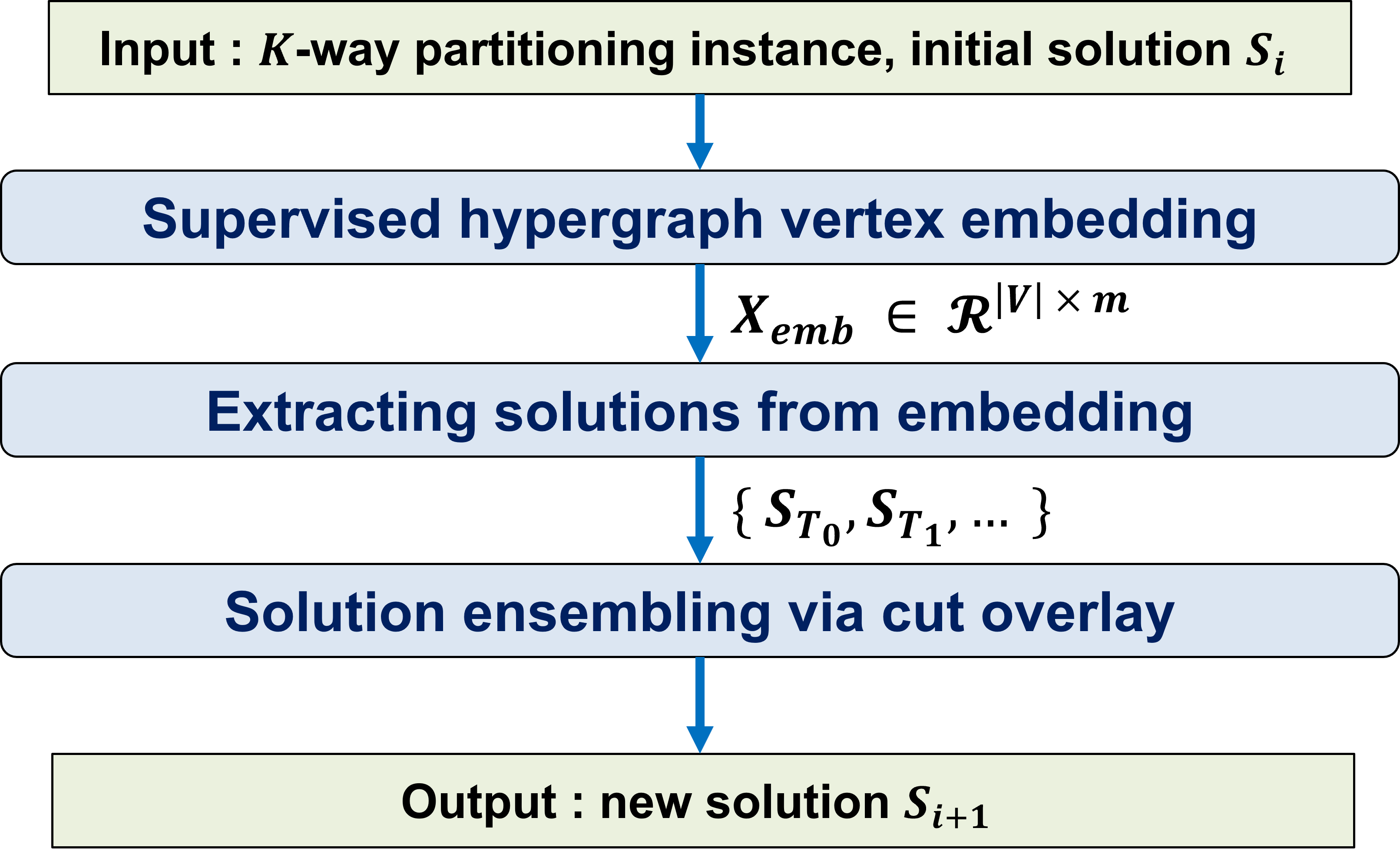
Figure 1: One iteration of K-SpecPart. The three modules are expanded in Figures 3, 5 and 6, and further described in Sections IV-VI. The initial partitioning solution $S_{0}$ can be obtained from any partitioner, but in this work, we use hMETIS and KaHyPar. During its iterations K-SpecPart collects its outputs $\{S_{0},S_{1},\ldots,S_{\beta}\}$. K-SpecPart then applies the ensembling module on $\{S_{0},S_{1},\ldots,S_{\beta}\}$ to compute its final output $S_{out}$.

The input is the hypergraph $H$ and a partitioning solution $S_{i}$ in the form of block labels $\{0,\ldots,K-1\}$ for the vertices. The vertex embedding module computes a map of each hypergraph vertex to a point in a low-dimensional space. The embedding is computed by a supervised algorithm, using $S_{i}$ as the supervision input [Alg. 1, Lines 7-19]. The intuition is that the vertex embedding is incentivized to conform with $S_{i}$, thus staying in the “vicinity” of $S_{i}$, but simultaneously to respect the global structure of the hypergraph, thus having the potential to improve $S_{i}$. The solution extraction module computes a pool of different partitioning solutions $\{S_{i,1}\ldots,S_{i,\delta}\}$ [Lines 20-22]. These are then sent to the ensembling module, which uses our cut-overlay method to convert the given solutions to a small instance of the $K$-way partition which can be solved much more reliably by more expensive partitioning algorithms [Line 23]. The solution to this small problem instance is then “lifted” (i.e., mapping back to the original hypergraph $H$) and further refined to the output $S_{i+1}$. The rest of this paper presents our implementations of these three modules.

Input: Hypergraph $H(V,E)$, Number of blocks $K$,

   Initial partitioning solution $S_{init}$,

   Number of supervision iterations $\beta$,

   Allowed imbalance between blocks $\epsilon$

Output: Improved partitioning solution $S_{out}$

1 Construct the clique expansion graph $G$ of $H$ and the Laplacian matrix $L_{G}$ of $G$ (Section IV)

2 Construct the weight-balance graph $G_{w}$ of $H$ and the Laplacian matrix $L_{G_{w}}$ of $G_{w}$ (Section IV)

3 Initialize the empty candidate solution list $\{S_{candidate}\}$

4 $\{S_{candidate}\}.push\_back(S_{init})$

5 $S_{0}=S_{init}$

6 for $i=0$; $i<\beta$ ; $i++$ do

       /* Supervised hypergraph vertex embedding (Section IV) */

7       if $K=2$ then

8             Construct the hint graph $G_{h}$ based on $S_{i}$ and the Laplacian matrix $L_{G_{h_{i}}}$ of $G_{h}$ (Section IV-A)

9             Solve the generalized eigenvalue problem $L_{G}x=\lambda(L_{G_{w}}+L_{G_{h_{i}}})x$ to obtain the first $m$ nontrivial eigenvectors $X_{emb}\in\mathcal{R}^{|V|\times m}$

10       end if

11      else

12             Decompose the $K$-way partitioning solution $S_{i}$ into $K$ bipartitioning (2-way) solutions $\{S_{b_{0}},...,S_{b_{K-1}}\}$ (Section IV-B)

13             for $j=0$; $j<K$; $j++$ do

14                   Construct the hint graph $G_{h_{j}}$ based on $S_{b_{j}}$ and the Laplacian matrix $L_{G_{h_{j}}}$ of $G_{h_{j}}$ (Section IV-B)

15                   Solve the generalized eigenvalue problem $L_{G_{j}}x=\lambda(L_{G_{w}}+L_{G_{h_{j}}})x$ to obtain the first $m$ nontrivial eigenvectors $X_{j}^{m}\in\mathcal{R}^{|V|\times m}$

16                  

17             end for

18            $X_{emb}=[X_{0}^{m}|X_{1}^{m}|...|X_{K-1}^{m}]$

19             Perform linear discriminant analysis (LDA) to generate the vertex embedding $X_{emb}\in\mathcal{R}^{|V|\times m}$.

20       end if

      /* Extracting solutions from embedding (Section V) */

21       Construct a family of trees $\{T_{0},T_{1},...\}$ leveraging the vertex embedding $X_{emb}\in\mathcal{R}^{|V|\times m}$

22       Generate hypergraph partitioning solutions $\{S_{T_{0}},S_{T_{1}},...\}$ through cut distilling and tree partitioning

23       Refine $\{S_{T_{0}},S_{T_{1}},...\}$ using multi-way FM

       /* Solution ensembling via cut overlay (Section VI) */

24       $S_{i+1}\leftarrow$ perform cut-overlay clustering and ILP-based partitioning on the top $\delta$ solutions from $\{S_{T_{0}},S_{T_{1}},...\}$

25       $\{S_{candidate}\}.push\_back(S_{i+1})$

26      

27 end for

/* Solution ensembling via cut overlay */

28 $S_{out}\leftarrow$ perform cut-overlay clustering and ILP-based partitioning on solutions $\{S_{candidate}\}$

29 Refine $S_{out}$ using multi-way FM

30 return $S_{out}$

Algorithm 1 K-SpecPart framework.

IV Supervised Vertex Embedding

The supervised vertex embedding module takes as inputs the hypergraph $H(V,E)$ and a $K$-way partitioning solution $S_{hint}$, and outputs an $m$-dimensional embedding $X^{|V|\times m}$.

In K-SpecPart, we use a spectral embedding algorithm that encodes into a generalized eigenvalue problem the supervision information $S_{hint}$. Figure 2 illustrates how the inclusion of the hint incentivizes the computation of an embedding that in general respects (spatially) the given solution $S_{hint}$, but also identifies vertices of contention where improving the solution may be possible.

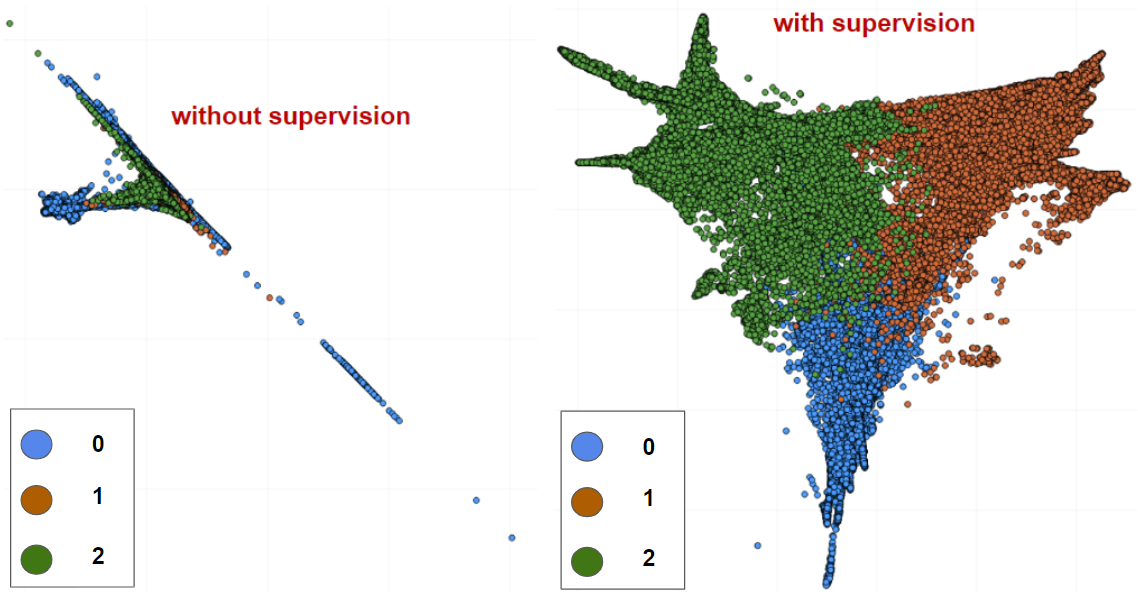
Figure 2: Vertex embeddings of the ISPD IBM14 benchmark. Point colors indicate block membership in a $3$-way partitioning solution with $\epsilon$ $=$ $5\%$ computed by hMETIS. The embedding on the right uses as a hint the same hMETIS solution, while the embedding on the left is unsupervised.

IV-A Embedding From Two-way Hint

The embedding algorithm for two-way hints is identical to that used in SpecPart [31]. The steps of the algorithm are shown in Figure 3 and described in following paragraphs that reprise for completeness the corresponding sections in [31].

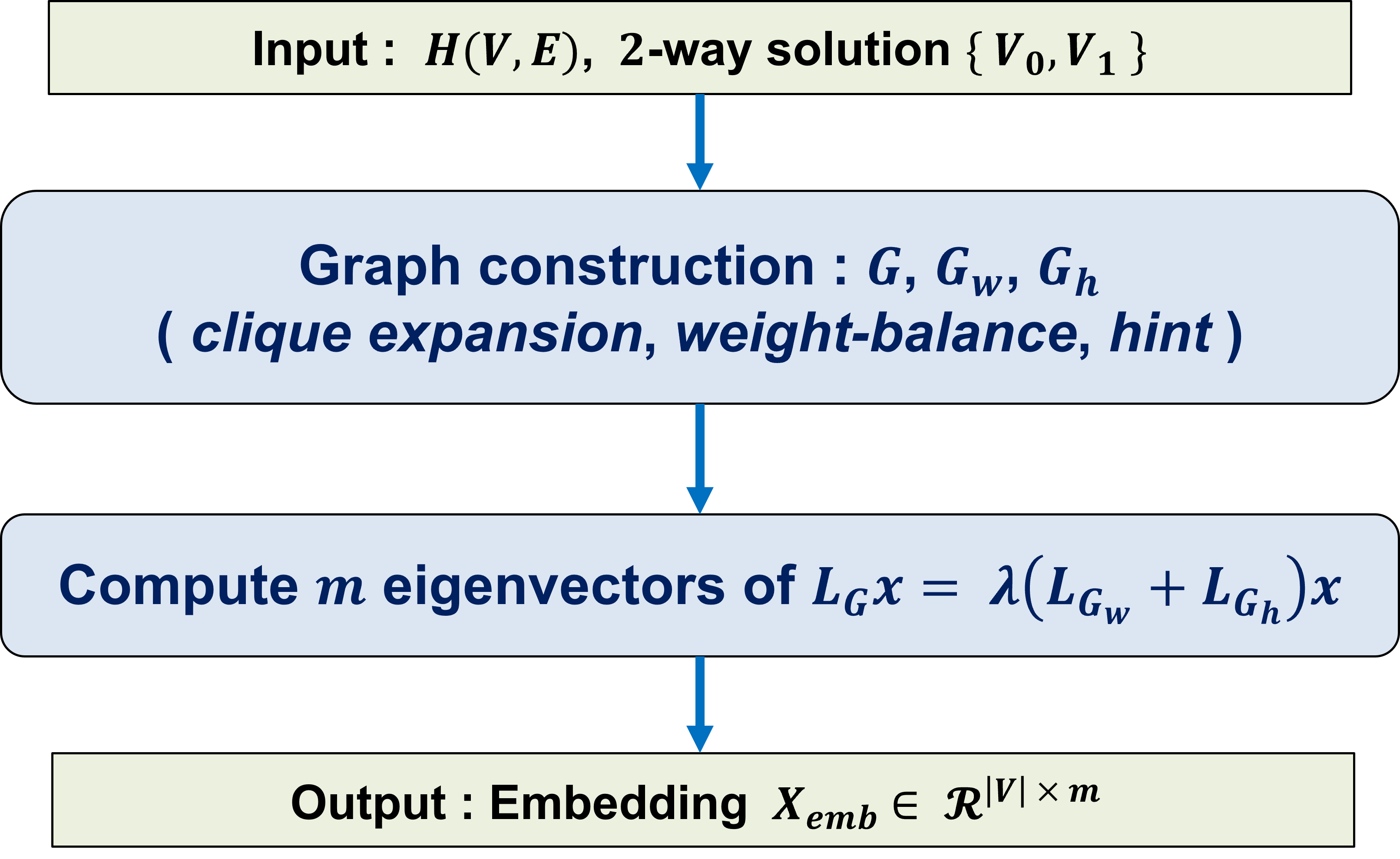
Figure 3: Supervised embedding with a two-way hint.

Graph Construction. We define the graphs used by the embedding algorithm: clique expansion graph $G$, weight-balance graph $G_{w}$ and hint graph $G_{h}$. An illustration of these graphs is given in Figure 4.

$\bullet$ Clique Expansion Graph $G$: A superposition of weighted cliques. The clique corresponding to the hyperedge $e\in E$ has the same vertices as $e$ and edge weights $\frac{1}{|e|-1}$. Graph $G$ has size $\sum_{e\in E}{\frac{|e|(|e|-1)}{2}}$ where $|e|$ is the size of hyperedge $e$. This is usually quite large relative to the input size $|I|=\sum_{e\in E}|e|$. For this reason, we only construct a function $f_{L_{G}}$ that evaluates matrix-vector products of the form $L_{G}x$, where $L_{G}$ is the Laplacian of $G$, which is all we need to perform the eigenvector computation. In all places where we mention the construction of any Laplacian, we construct the equivalent function for evaluating matrix-vector products. The function $f_{L_{G}}$ is an application of the following equation that is based on expressing $L_{G}$ as a sum of Laplacians of cliques:

where ${\bf 1_{e}}$ is the 1-0 vector with 1s in the entries corresponding to the vertices in $e$. By exploiting the sparsity in ${\bf 1_{e}}$, the product is implemented to run in $O(|I|)$ time.

$\bullet$ Weight-Balance Graph $G_{w}$: A complete weighted graph used to capture arbitrary vertex weights and incentive balanced cuts. $G_{w}$ has the same vertices as hypergraph $H$, and edges of weight $w_{u}\cdot w_{v}$ between any two vertices $u$ and $v$. Let $W_{V_{i}}$ be the weight of block $V_{i}$, i.e., $W_{V_{i}}=\sum_{v\in V_{i}}{w_{v}}.$ Then, given a two-way solution $S_{b}=\{V_{0},V_{1}\}$, we have

$$\begin{split}W_{V_{0}}\cdot W_{V_{1}}&=\sum_{v\in V_{0}}{w_{v}}\cdot\sum_{u\in V_{1}}{w_{u}}=\sum_{v\in V_{0},u\in V_{1}}{w_{v}\cdot w_{u}}\\ &=\sum_{v\in V_{0},u\in V_{1}}{w_{e_{vu}}}=cutsize_{G_{w}}(S_{b}).\end{split}$$ (5)

We now discuss how to compute matrix-vector products with the Laplacian matrix of $G_{w}$. Let ${\bf w}$ be the vector of vertex weights. We apply the identity

$$L_{G_{w}}x={\bf w}\circ x-\frac{x^{T}{\bf 1}}{1^{T}\bf 1}\cdot{\bf w}$$ (6)

where ${\bf 1}$ is the all-ones vector and $\circ$ denotes the Hadamard product. This can be carried out in time $O(|V|)$.

In general, any vector $x$ can be written in the form $x=y+c{\bf 1}$, where $y^{T}{\bf 1}=0$. Substituting this decomposition of $x$ into the above equation, we get that $L_{G_{w}}x={\bf w}\circ y.$ In other words, $L_{G_{w}}$ acts like a diagonal matrix on $y$ and nullifies the constant component of $x$.

$\bullet$ Hint Graph $G_{h}$: A complete bipartite graph on the two vertex sets $V_{0}$ and $V_{1}$ defined by the two-way hint solution $S_{{b}}$. We have

$$\begin{split}L_{G_{h}}x&=(x-\frac{x^{T}{\bf 1}}{1^{T}1}\cdot{\bf 1})-(x-\frac{x^{T}{\bf 1_{V_{0}}}}{1_{V_{0}}^{T}1_{V_{0}}}\cdot{\bf 1_{V_{0}}})\\ &-(x-\frac{x^{T}{\bf 1_{V_{1}}}}{1_{V_{1}}^{T}1_{V_{1}}}\cdot{\bf 1_{V_{1}}})\end{split}$$ (7)

where ${\bf 1}_{V_{i}}$ denotes the 1-0 vector with 1s in entries corresponding to the vertices in $V_{i}$. By exploiting the sparsity in ${\bf 1}_{V_{i}}$, the product is implemented in $O(|V|)$ time.

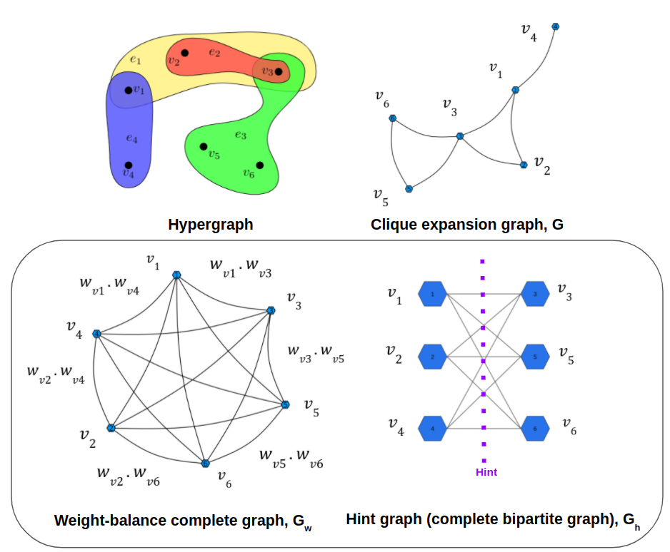
Figure 4: Graphs used for embedding generation.

Generalized Eigenvalue Problem and Embedding. Given a two-way partitioning solution $S_{hint}$, we solve the generalized eigenvalue problem $L_{G}x=\lambda Bx$ where $B=L_{G_{w}}+L_{G_{h}}$, and compute the first $m$ nontrivial eigenvectors $X\in{\mathbb{R}}^{|V|\times m}$ whose rows provide the vertex embedding.

From the discussion in Section II-B recall that the eigenvalue problem is directly related to solving

$$\min_{x}R(x)=\min_{x}\frac{x^{T}L_{G}x}{x^{T}L_{G_{w}}x+x^{T}L_{G_{h}}x}$$ (8)

over the real vectors $x$. Recall also that this is a relaxation of the problem over 0-1 indicator vectors. Let $x_{S}$ be the indicator vector for some set $S\subset V$. Then, using Equation (1) we can understand the rationale for Equation (8):

• $x_{S}^{T}L_{G}x_{S}=cutsize_{G}(S)$ which is a proxy for $cutsize_{H}(S_{b})$. Thus, the numerator incentivizes smaller cuts in $H$.

• $x_{S}^{T}L_{G_{w}}x_{S}=cutsize_{G_{w}}(S)$. By Equation (5), this is equal to $W_{S}\cdot W_{V-S}$, where $W_{S}$ is the total weight of the vertices in $S$. Thus, the denominator incentivizes a large $W_{S}\cdot W_{V-S}$, which implies balance.

• $x_{S}^{T}L_{G_{h}}x_{S}$ is maximized when all edges of $G_{h}$ are cut. Thus, the denominator incentivizes cutting many edges that are also cut by the hint.

Generalized Eigenvector Computation. We solve $L_{G}x=\lambda Bx$ using LOBPCG, an iterative preconditioned eigensolver. LOBPCG relies on functions that evaluate matrix-vector products with $L_{G}$ and $B$. For fast computation, the solver can utilize a preconditioner for $L_{G}$, also in an implicit functional form. To compute the preconditioner we first obtain an explicit graph $\tilde{G}$ that is spectrally similar with $G$ and has size at most $2|I|$, where $|I|=\sum_{e\in E}|e|$. More specifically, we build $\tilde{G}$ by replacing every hyperedge $e$ in $H$ with the sum of 2 uniformly weighted random cycles on the vertices $V_{e}$ of $e$. This is an essentially optimal sparse spectral approximation for the clique on $V_{e}$, as implied from asymptotic properties of random $d$-regular expanders (e.g., see [40] or Theorem 4.16 in [41]). Since $G$ is a sum of cliques, and $\hat{G}$ is a sum of tight spectral approximations of cliques, graph support theory [46] implies that $\hat{G}$ is a tight spectral approximation for $G$. Finally, we compute a preconditioner of $L_{\hat{G}}$ using the CMG algorithm [23] and in particular the implementation from [55]. By transitivity [46] the preconditioner for $L_{\hat{G}}$ is also a preconditioner for $L_{G}$.

IV-B Embedding From Multi-way Hint

The flow for generating an $m$-dimensional embedding from a $K$-way hint is shown in Figure 5. The steps are described in the following paragraphs.

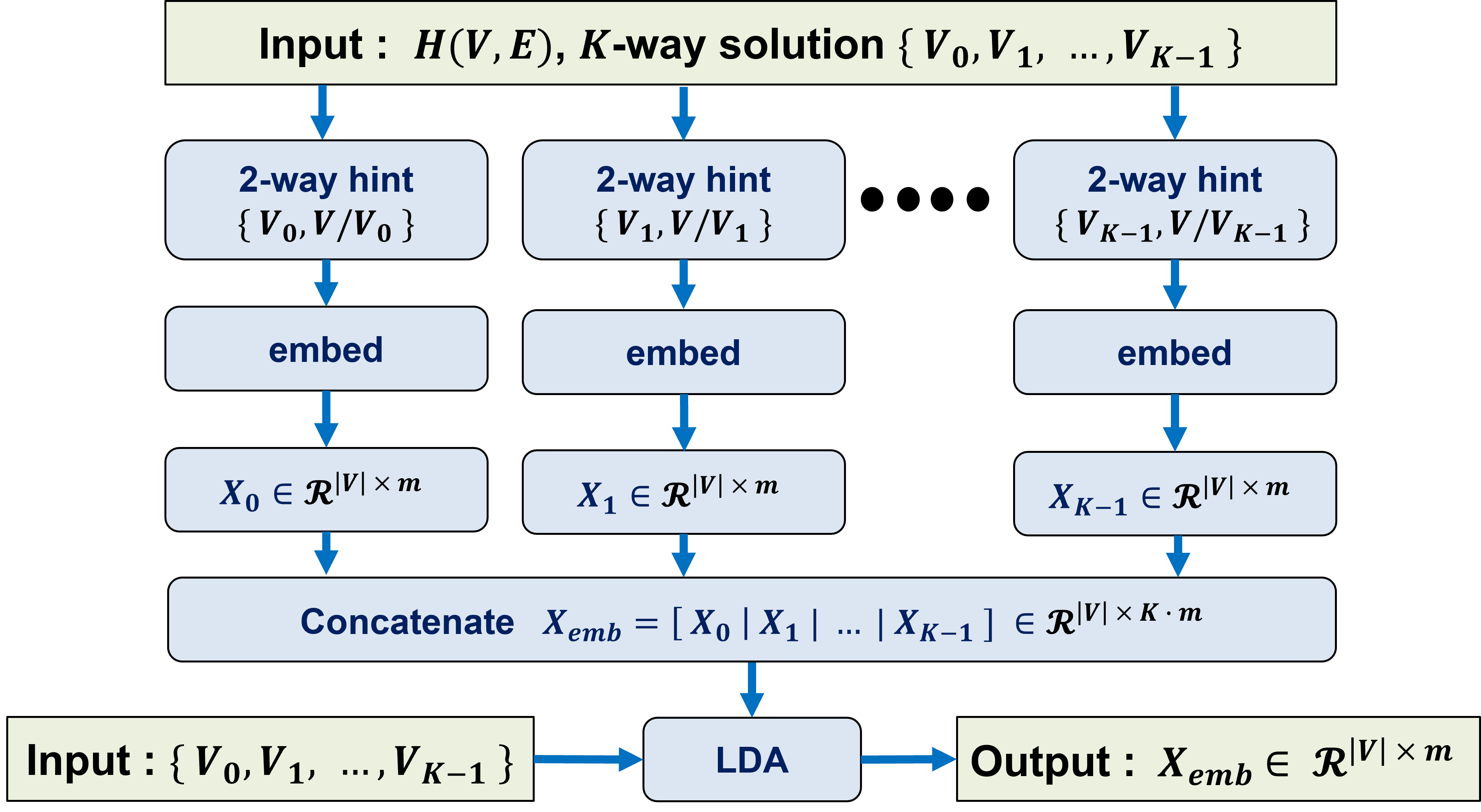
Figure 5: Vertex embedding generation process for a given multi-way ($K$ $>$ $2$) hint, using the two-way embedding subroutine from Section IV-A.

Embedding by concatenation. In the $K$-way case where $K>2$, the solution hint $S_{hint}$ corresponds to a $K$-way partitioning solution $\{V_{0},\ldots,V_{K-1}\}$. We then extract $K$ different bipartitions, $S_{b_{i}}$, for $i=0,\ldots,K-1$, where

$$S_{b_{j}}=\{V_{j},\bigcup_{i=0,i\neq j}^{K-1}V_{i}\}.$$

For each $S_{b_{j}}$ we solve an instance of the generalized problem we set up in Section IV-A. This generates $K$ different embeddings $X_{j}\in{\mathbb{R}}^{|V|\times m}$. We then concatenate these $K$ embeddings horizontally to get our final embedding $X_{emb}\in{\mathbb{R}}^{|V|\times{K\cdot m}}$, i.e.,

$$X_{emb}=[X_{0}|X_{1}|\ldots|X_{K-1}],~{}\textnormal{where~{}}X_{j}\in{\mathbb{R}}^{|V|\times m}.$$

Supervised Dimensionality Reduction. Note that the above embedding $X_{emb}$ has dimension $K\cdot m$. We then apply on $X_{emb}$ a supervised dimensionality reduction algorithm, specifically LDA (see Section VII-E), as illustrated in Figure 5. We use LDA primarily to reduce the runtime of subsequent steps, but also because this second application of supervision has the potential to increase the quality of the embedding.

Besides $X_{emb}$, LDA takes as input a target dimension, and class labels for the points in $X_{emb}$. We choose $m$ as the target dimension. We assign label $i$ to vertex $v$ if $V\in V_{i}$. For the computation, we use a Julia-based LDA implementation from the MultivariateStats.jl package [54].

V Extracting Solutions from Embeddings

The inputs of the solution extraction module are the hypergraph $H$, number of blocks $K$, balance constraint $\epsilon$ and an embedding $X_{emb}\in\mathcal{R}^{|V|\times m}$, and the output is a pool of solutions $\{S_{0},\ldots,S_{\delta-1}\}$. The main idea of the algorithm is to use the embedding to reduce the $K$-way hypergraph partitioning problem to multiple $K$-way balanced partitioning problems on trees whose edge weights “summarize” the underlying cuts of the hypergraph. The steps of the algorithm are shown in Figure 6 and described in Sections V-C and V-B.

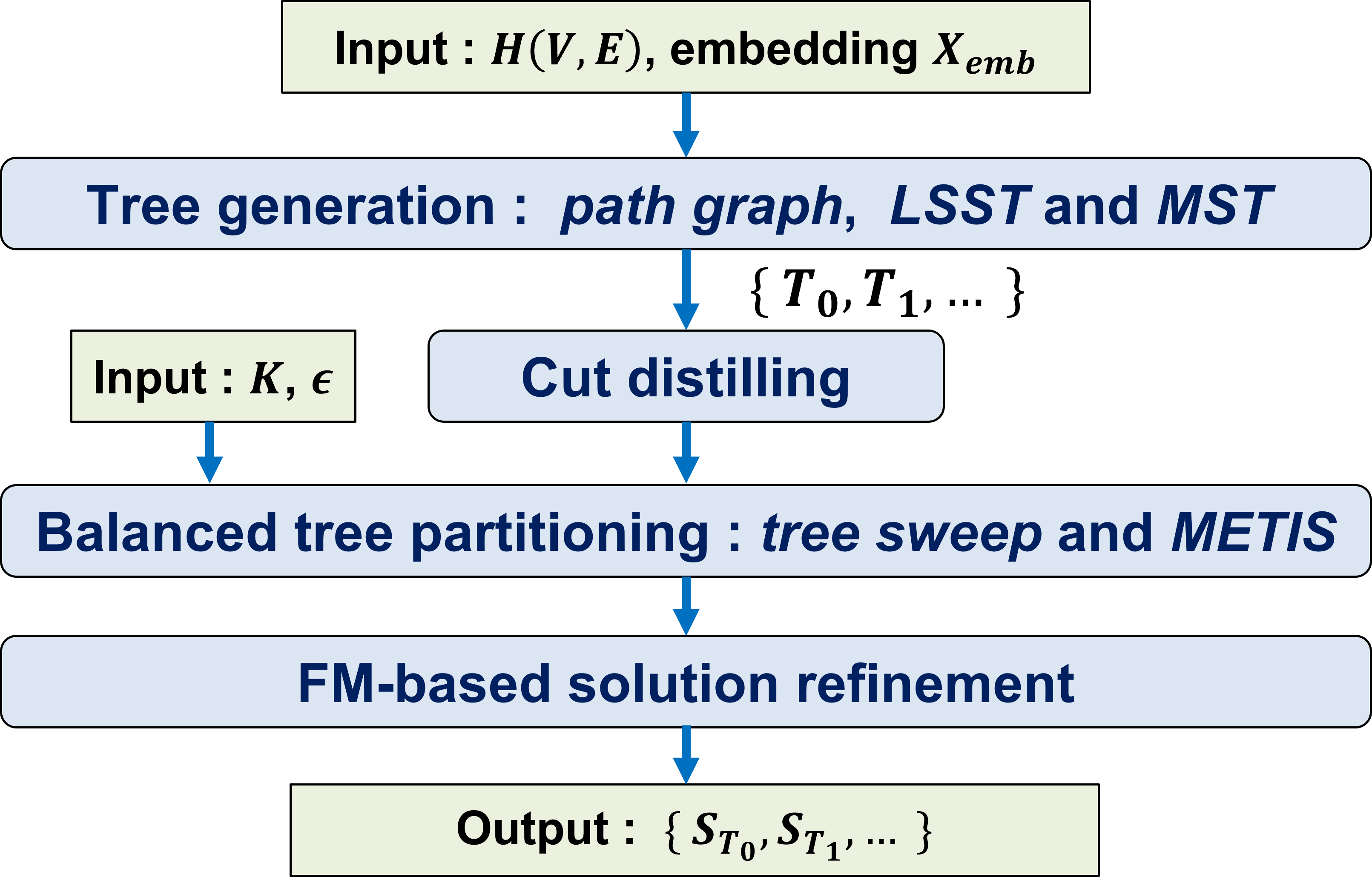
Figure 6: The flow of extracting solutions from embeddings.

V-A Tree Generation

In our algorithm, each $S_{i}$ in the output comes from a tree that spans the set of vertices $V$. Here we define the types of trees we use.

Path Graph. We first define a path graph on the vertices $V$, which appears in the proofs of Cheeger inequalities for bipartitioning [38, 39]. Let $X_{emb_{i}}$ be the $i^{th}$ column of $X$. We sort the values in $X_{emb_{i}}$ and let $o(j)$ be vertex at the $j^{th}$ position of the sorted $X_{emb_{i}}$. Then we define the path graph on $V$ to be $v_{o(1)},v_{o(2)},\ldots,v_{o(|V|)}.$

Clique Expansion Spanning Tree. The path graph is likely not a spanning tree of the clique expansion graph $G$. To take connectivity directly into account, we work with a weighted graph that reflects both the connectivity of $H$ and the global information contained in the embedding, adapting an idea that has been used in work on $K$-way Cheeger inequalities [25]. Concretely, we form a graph $\hat{G}$ by replacing every hyperedge $e$ of $H$ with a sum of $\zeta$ cycles (as also done in Section IV-A). Suppose that $Y\in{\mathbb{R}}^{|V|\times d}$ is an embedding matrix. We denote by $Y_{u}$ the row of $Y$ containing the embedding of vertex $u$. We construct the weighted graph $\hat{G}_{Y}$ by setting the weight of each edge $e_{uv}\in\hat{G}$ to $||Y_{u}-Y_{v}||_{2}$, i.e., equal to the Euclidean distance between the two vertices in the embedding. Using $\hat{G}_{Y}$ we build two spanning trees.

$\bullet$ LSST: A desired property for a spanning tree $\hat{T}$ of $\hat{G}_{Y}$ is to preserve the embedding information contained in $\hat{G}$ as faithfully as possible. Thus, we let $\hat{T}$ be a Low Stretch Spanning Tree (LSST) of $\hat{G}$, which by definition means that the weight $w_{e_{uv}}$ of each edge in $\hat{G}$ is approximated on average, and up to a small function $f(|V|)$, by the distance between the nodes $u$ and $v$ in $\hat{T}$ [2]. We compute the LSST using the AKPW algorithm of Alon et al. [2]. The output of the AKPW algorithm depends on the vertex ordering of its input. To make it invariant to the vertex ordering in the original hypergraph $H$, we relabel the vertices of $\hat{G}_{Y}$ using the order induced by sorting the smallest nontrivial eigenvector computed earlier. Empirically, this order has the advantage of producing LSSTs that contain slightly better cutsizes.

$\bullet$ MST: A graph can contain multiple different LSSTs, with each of them approximating to different degrees the weight $w_{e_{uv}}$ for any given $e_{uv}$. It is known that the AKPW algorithm is suboptimal with respect to the approximation factor $f(|V|)$; more sophisticated algorithms exist but they are far from practical. Hence, we also apply Kruskal’s algorithm [3] to compute a Minimum Spanning Tree of $\hat{G}$, which serves as an easy-to-compute proxy to an LSST. The MST can potentially have better or complementary distance-preserving properties relative to the tree computed by the AKPW algorithm.

In summary, we compute $m$ path graphs, and also generate the LSSTs and MSTs by letting $Y$ range over each subset of columns of $X_{emb}$. This produces a family of $t=2(2^{m}-1)+m$ trees.

V-B Cut Distilling

We reweight each tree $T$ in the given family of trees to distill the cut structure of $H$ over $T$, in the following sense. (i) For a given tree $T=(V,E_{T})$, observe that the removal of an edge $e_{T}$ of $T$ yields a partitioning $S_{e_{T}}$ of $V$ and thus of the original hypergraph $H$. (ii) We reweight each edge $e_{T}\in E_{T}$ with the corresponding $cutsize_{H}(S_{e_{T}})$.

With this choice of weights, we have $cutSize_{H}(S)\leq cutSize_{T}(S)$, and owing to the reasoning behind the construction of $T$, $cutSize_{T}(S)$ provides a proxy for $cutSize_{H}(S)$.

Computing edge weights on $T$ can be done in $O(\sum_{e}|e|)$ time, via an algorithm involving the computation of least common ancestors (LCA) on $T$, in combination with dynamic programming on $T$ [7]. We provide pseudocode in Algorithm 2 and give a fast implementation in [49]. We illustrate the idea using the example in Figure 7.

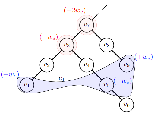
Figure 7: Hyperedge, junctions and their numerical labels. The vertices highlighted in red are the junction vertices.

.

We consider $T$ to be rooted at an arbitrary vertex. In the example of Figure 7, consider hyperedge $e=\{v_{1},v_{5},v_{9}\}$. The LCA of its vertices is $v_{7}$. Then, the weight of $e$ should be accounted for the set $C_{e}\subset E_{T}$ of all tree edges that are ancestors of $\{v_{1},v_{5},v_{9}\}$ and descendants of $v_{7}$. We do this as follows [Alg. 2, Lines 2-13]. (i) We compute a set of junction vertices that are LCAs of $\{v_{1},v_{5}\}$ and $\{v_{1},v_{5},v_{9}\}$. (ii) We then “label” these junctions with $-w_{e}$, where $w_{e}$ is the weight of $e$. More generally, for a hyperedge $e=\{v_{i_{1}},\ldots,v_{i_{p}}\}$ ordered according to the post-order depth-first search traversal on $T$, we calculate the LCAs for the $p-1$ sets $\{v_{i_{1}},\ldots,v_{i_{j}}\}$ for $j=2,\ldots,p$, and the junctions are labeled with appropriate negative multiples of $w_{e}$. We also label the vertices in $e$ with $w_{e}$. (iii) All other vertices are labeled with 0.

Input: Hypergraph $H(V,E)$, Tree $T(V,E_{T})$

Output: Tree $T$ with updated edge weights

1 Select an arbitrary vertex $v_{root}$ from $V$ and root $T$ at $v_{root}$

2 Perform a post-order depth-first search traversal on $T$ and store the sequence of visited vertices in $visited\_sequence$

/* Label each vertex in $T$ based on the hyperedge weight $w_{e}$ for $e\in E$ */

3 $cuts\_{delta}[v]\leftarrow 0$ for all $v$ in $V$

4 for each $e$ in $E$ do

5       $cuts\_{delta}[v]=cuts\_{delta}[v]+w_{e}$ for all $v$ in $e$

6       $\{v_{i0},...,v_{i(|e|-1)}\}\leftarrow$ arrange the vertices of $e$ according to their positions in $visited\_sequence$

7       $v_{LCA}\leftarrow$ $v_{i0}$

8       for $j=1$; $j<|e|$; $j++$ do

9             $v_{LCA}\leftarrow$ identify the least common ancestor (LCA) for $v_{LCA}$ and $v_{ij}$ in $T$

10             $cuts\_{delta}[v_{LCA}]$ = $cuts\_{delta}[v_{LCA}]-w_{e}$

11            

12       end for

13      $cuts\_{delta}[v_{LCA}]$ = $cuts\_{delta}[v_{LCA}]-w_{e}$

14      

15 end for

/* Reweight edges of $T$ */

16 for each $e_{T}$ in $E_{T}$ do

17       $w_{e_{T}}\leftarrow$ compute the sum-below-$e_{T}$ (i.e., the sum of the labels $cuts\_{delta}$ of vertices that are descendants of $e_{T}$) in the post-order depth-first search ordering

18      

19 end for

20return $T$ with updated edge weights

Algorithm 2 Cut Distilling

Consider then an arbitrary edge $e_{T}$ of the tree, and compute the sum-below-$e_{T}$, i.e., the sum of the labels of vertices that are descendants of $e_{T}$. This will be $w_{e}$ on all edges of $C_{e}$ and 0 otherwise, thus correctly accounting for the hyperedge $e$ on the intended set of edges $C_{e}$ [Alg. 2, Lines 14-16]. In order to compute the correct total counts of cut hyperedges on all tree edges, we iterate over hyperedges, compute their junction vertices, and aggregate the associated labels. Then, for any tree edge $e_{T}$, the sum-below-$e_{T}$ will equal $cutsize_{H}(S_{e_{T}})$. These sums can be computed in $O(|V|)$ time, via dynamic programming on $T$.

V-C Tree Partitioning

We use a linear “tree-sweep” method and METIS to partition the trees. In our studies, we have observed that only using METIS as the tree partitioner results in an average of 3%, 4% and 3% deterioration in cutsize for $K=$ 2, 3 and 4 respectively.

$\bullet$ $K$ $=$ $2$. Given a cut-distilling tree $T$, and referring back to Figure 7, an application of dynamic programming can compute the total weight of the vertices that lie below $e_{T}$ on $T$. We can thus compute the value for the balanced cut objective for $S_{e_{T}}$ and pick the $S_{e_{T}}$ that minimizes the objective among the $n-1$ cuts suggested by the tree. This “tree-sweep” algorithm generates a good-quality two-way partitioning solution from the tree. Additionally, we use METIS [5] to solve a balanced two-way partitioning problem on the edge-weighted tree, with the original vertex weights from $H$. In some cases, this improves the solution.

$\bullet$ $K$ $>$ $2$. Similar to $K=2$, we use two algorithms to compute two potentially different $K$-way partitioning solutions of the tree. The first algorithm is METIS [5]. The second algorithm extends the two-way cut partitioning of the tree to $K$-way partitioning. To this end, we apply the two-way algorithm recursively, for $K$ $-$ $1$ levels. We use a similar idea as the VILE (“very illegal”) method [37] to generate an imbalanced partitioning solution and then refine the solution with the FM algorithm. Specifically, while computing the $i^{th}$ level bipartitioning solution $S_{e_{T}}^{i}$ on the tree $e_{T}$, the balance constraint for block $V_{i0}$ in the bipartitioning solution $S(V_{i0},V_{i1})$ is: $(\frac{1}{K}-\epsilon)\cdot W\leq\sum_{v\in V_{i0}}{w_{v}}\leq(\frac{1}{K}+\epsilon)\cdot W$.

After obtaining the $i^{th}$ bipartitioning solution $S(V_{i0},V_{i1})$, we mark all the vertices in $V_{i0}$ as fixed vertices and set their weights to zero. We then proceed with the $(i+1)^{th}$ level bipartitioning solution $S_{e_{T}}^{i+1}$ on the tree $e_{T}$.

V-D Refinement on the hypergraph

The previous step solves balanced partitioning on trees that share the same vertex set $V$ with $H$. Note that the number of solutions will be larger than the number of trees $t$, because we apply different partitioning algorithms to each tree. These solutions are then transferred to $H$, and each is further refined using the FM algorithm [13] on the entire hypergraph $H$. In particular, we use the FM implementation in [50].

VI Solution ensembling via cut overlay

The input of this module is the given $K$-way partitioning instance and a pool of partitioning solutions. We then perform the following steps.

Cut-Overlay Clustering. We first select the $\delta$ best solutions. Let $E_{1},\ldots,E_{\delta}\subset E$ be the sets of hyperedges cut in the $\delta$ solutions. We remove the union of these sets from $H$ to yield a number of connected clusters. Then, we perform a cluster contraction process that is standard in multilevel partitioners, to give rise to a clustered hypergraph $H_{c}(V_{c},E_{c})$. By construction, $E_{c}$ consists of $E_{1}\cup...\cup E_{\delta}$ and hence is guaranteed to contain a solution which is at least as good as the best among the cuts $E_{i}$.

ILP-based Partitioning. The coarse hypergraph ($H_{c}$) obtained from cut-overlay clustering usually has a few hundreds of vertices and hyperedges (including with the default setting $\delta=5$). While even this small size would be expected to be prohibitive for applying an exact optimization algorithm, somewhat surprisingly, an ILP formulation can frequently solve the problem optimally. In most cases, our ILP produces a solution better than any of the $\delta$ candidate solutions. We solve the ILP with the CPLEX solver [44]. We have found that the open-source OR-Tools package [53] is significantly slower. In our current implementation, we include a parameter $\gamma$: in the case when the number of hyperedges in $H_{c}$ is larger than $\gamma$, we run hMETIS on $H_{c}$. This step generates a $K$-way solution $S^{\prime}$ on $H_{c}$.

Lifting and Refinement. The solution $S^{\prime}$ from the previous step is “lifted” to $H$, with the standard lifting process that multilevel partitioners use. Finally, we apply FM refinement on $H$ to obtain the final solution $S$. Here we again use the FM implementation from [50].

VII Experimental Validation

The K-SpecPart framework is implemented in Julia. We use CPLEX [44] and LOBPCG [20] as our ILP solver (we provide an OR-Tools based implementation) and eigenvalue solver respectively. We run all experiments on a server with an Intel Xeon E5-2650L, 1.70GHz CPU and 256 GB memory. We have compared our framework with two state-of-the-art hypergraph partitioners (hMETIS [6] and KaHyPar [29]) on the ISPD98 VLSI Circuit Benchmark Suite [4] and the Titan23 Suite [9]. We make public all partitioning solutions, scripts and code at [49].

VII-A Cutsize Comparison

We run hMETIS and KaHyPar with their respective default parameter settings. We denote by hMETIS_t, the best cutsize obtained by $t$ runs of hMETIS, with $t$ different seeds. We denote by hMETIS_avg, the average (over 50 samples) cutsize of hMETIS₂₀. We adopt similar notation for KaHyPar. In all our experiments we run K-SpecPart with its default settings (see Table I) and a hint that comes from hMETIS₁. We compare K-SpecPart against hMETIS₅ and KaHyPar₅; this is because 5 runs of hMETIS have a similar runtime with K-SpecPart. For a more robust and challenging comparison, we also compare K-SpecPart against hMETIS_avg and KaHyPar_avg, which gives to these partitioners at least $\sim$4X the walltime of K-SpecPart.

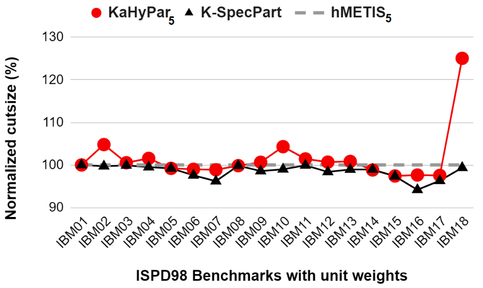
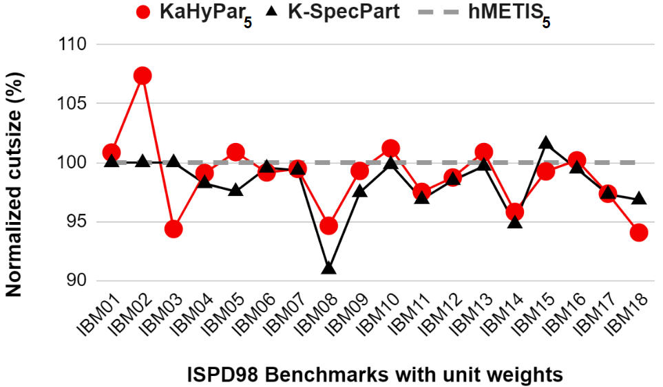
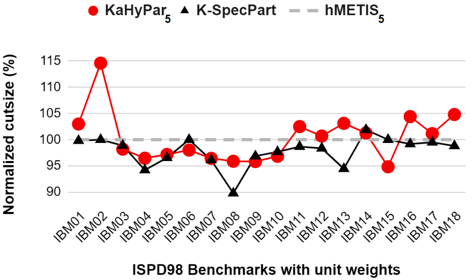
Figure 8: K-SpecPart results on the ISPD98 Benchmarks [4] with unit vertex weights for $\epsilon=2\%$. Top to bottom: $K=2,3,4$.

ISPD98 Benchmarks with Unit Weights. Comparisons with hMETIS₅ and KaHypar₅ are presented in Figure 8. K-SpecPart significantly improves over both hMETIS₅ and KaHyPar₅ on numerous benchmarks for both two-way and multi-way partitioning. Comparisons with hMETIS_avg and KaHyPar_avg are reported in Table III. Each average value is rounded to the nearest tenth (0.1). We observe that K-SpecPart generates better partitions ($\sim$2% better on some benchmarks) than hMETIS_avg and KaHyPar_avg on the majority of ISPD98 testcases.

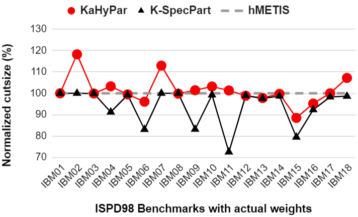
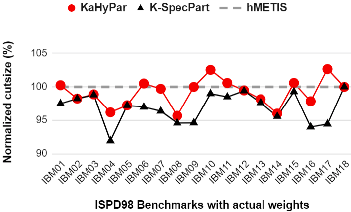
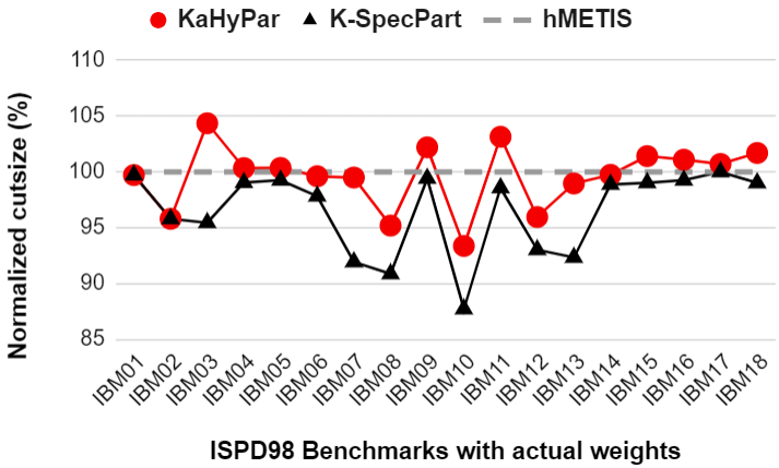
Figure 9: K-SpecPart results on the ISPD98 Benchmarks [4] with actual vertex weights for $\epsilon=2\%$. Top to bottom: $K=2,3,4$. Cutsizes are normalized with respect to those by hMETIS₅.

ISPD98 Benchmarks with Actual Weights. The inclusion of weights makes the problem more general and potentially more challenging. Figure 9 compares K-SpecPart against hMETIS₅ and KaHyPar₅, while Table IV provides comparisons with hMETIS_avg and KaHyPar_avg. We see that K-SpecPart tends to yield more significant improvements relative to the unit-weight case. For example, for IBM11_w, K-SpecPart generates almost $27$% improvement over hMETIS and KaHyPar for $K=2$. We notice similar improvements for $K>2$ as seen on IBM04_w for $K=3$ and IBM10_w for $K=4$.

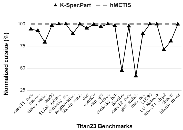
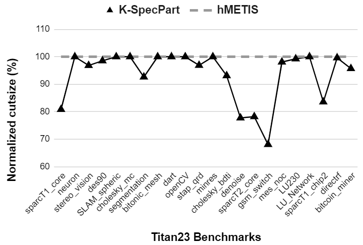
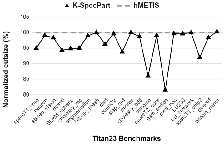
Figure 10: K-SpecPart results on the Titan23 Benchmarks [9] for $\epsilon=2\%$. Top-to-bottom: $K=2,3,4$. Cutsizes are normalized with respect to those by hMETIS₅.

Titan23 Benchmarks. The Titan23 benchmarks are interesting not only because they are substantially larger than the ISPD98 benchmarks, but also because they are generated by different, more modern synthesis processes. In some sense, they provide a “test of time” for hMETIS, as well as for KaHyPar which does not include Titan23 in its experimental study [29]. Figure 10 compares K-SpecPart against hMETIS₅, while Table V compares with hMETIS_avg. Although the K-SpecPart runtime is still similar to hMETIS₅, the runtime of KaHyPar on some of these benchmarks is exceedingly long (over two hours), making it unsuitable for any reasonable industrial setting (for more details on runtime, see [49]). For this reason we do not compare against KaHyPar. We observe that K-SpecPart generates better partitioning solutions compared to hMETIS₅ and hMETIS_avg. On gsm_switch in particular, K-SpecPart achieves more than 50% better cutsize.

VII-B Runtime Remarks

Our current Julia implementation of K-SpecPart has a walltime approximately 5X that of a single hMETIS run. K-SpecPart does utilize multiple cores, but there is still potential for speedup, in the following ways. (i) Most of the computational effort is in the embedding generation module. For $K>2$, K-SpecPart employs limited parallelism in the embedding generation module, by solving in parallel the $K$ eigenvector problem instances. The eigensolver has much more potential for parallelism since it relies on sequential and unoptimized sparse matrix-vector multiplications. These can be significantly speeded up on multicore CPUs, GPUs, or other specialized hardware. (ii) In the tree partitioning module, K-SpecPart uses parallelism to handle partitioning of multiple trees. The most time-consuming component of this module is the cut distillation algorithm, where there is scope for runtime improvement, especially for larger instances. This can be achieved by implementing the faster LCA algorithm in [7]. (iii) The CPLEX solver can also be accelerated by leveraging the “warm-start” feature where a previously computed partitioning solution can be used as an initial solution for the ILP. Furthermore, the CPLEX solver often computes a solution prior to its termination where extra time is spent to produce a computational proof of optimality [44]. Using a timeout is an option that can accelerate the solver without significantly affecting the quality of the output, but we have not explored this option in K-SpecPart.

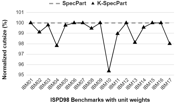
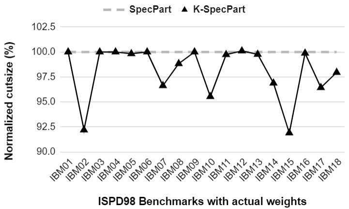
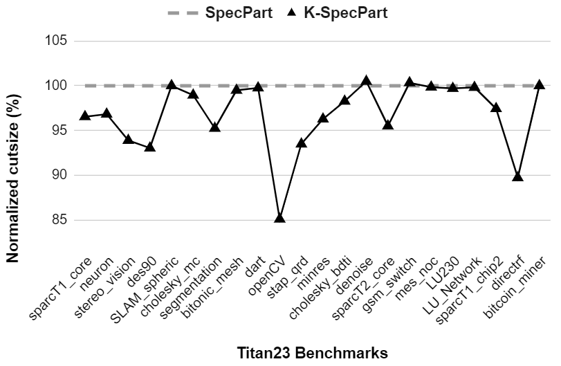
Figure 11: Comparison of K-SpecPart and SpecPart on the bipartitioning problem ($\epsilon$ = $2\%$). Top-to-bottom: ISPD98 with unit weights, ISPD98 with actual weights and Titan23.

VII-C K-SpecPart Improvements Over SpecPart

We have also compared K-SpecPart for the case $K=2$, against SpecPart [31]. The results are presented in Figure 11. Although SpecPart also improves the hint solutions from hMETIS and KaHyPar, we observe that K-SpecPart generates significant improvement (often in the range of $10$-$15$%) over SpecPart on various benchmarks. This improvement can be attributed to two main factors: (i) K-SpecPart refines the partitioning solutions generated from the constructed trees using a FM refinement algorithm; and (ii) K-SpecPart incorporates cut-overlay clustering and ILP-based partitioning in each iteration.

VII-D Parameter Validation

We now discuss the sensitivity of K-SpecPart with respect to its parameters, shown in Table II. We define the score value as the average improvement of K-SpecPart with respect to hMETIS_avg on benchmarks sparcT1_core, cholesky_mc, segmentation, denoise, gsm_switch and directf, for $K=2$ and $\epsilon=5\%$. With respect to $\gamma$, we have found that using hMETIS instead of ILP for partitioning (i.e., setting $\gamma=0$) worsens the score value by $2.68$%. We have also found that settings of $\gamma>500$ do not improve the score value. For the other parameters, we perform the following experiment. When we vary the value of one parameter (parameter sweep), the remaining parameters are fixed at their default values. The results are presented in Figure 12. From the results of tuning parameters on K-SpecPart we establish that our default parameter setting represents a local minimum in the hyperparameter search space.

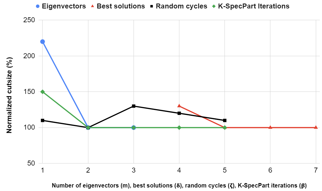
Figure 12: Validation of K-SpecPart parameters. (a) Number of eigenvectors ($m$) sweep; (b) number of best solutions ($\delta$) sweep; (c) number of iterations ($\beta$) sweep; and (d) number of random cycles ($\zeta$) sweep.

VII-E Effect of Linear Discriminant Analysis (LDA)

We have compared the cutsize and runtime of K-SpecPart with LDA, and K-SpecPart without LDA, i.e., utilizing the horizontally stacked eigenvectors $X_{emb}$. The result for multi-way partitioning ($K=4$) is presented in Figure 13. We observe that K-SpecPart with LDA generates slightly better ($\sim$1%) cutsize with significantly faster ($\sim$10X) runtime compared to K-SpecPart without LDA. However, for the case of bipartitioning ($K=2$) we do not observe any significant difference in cutsize when employing LDA.

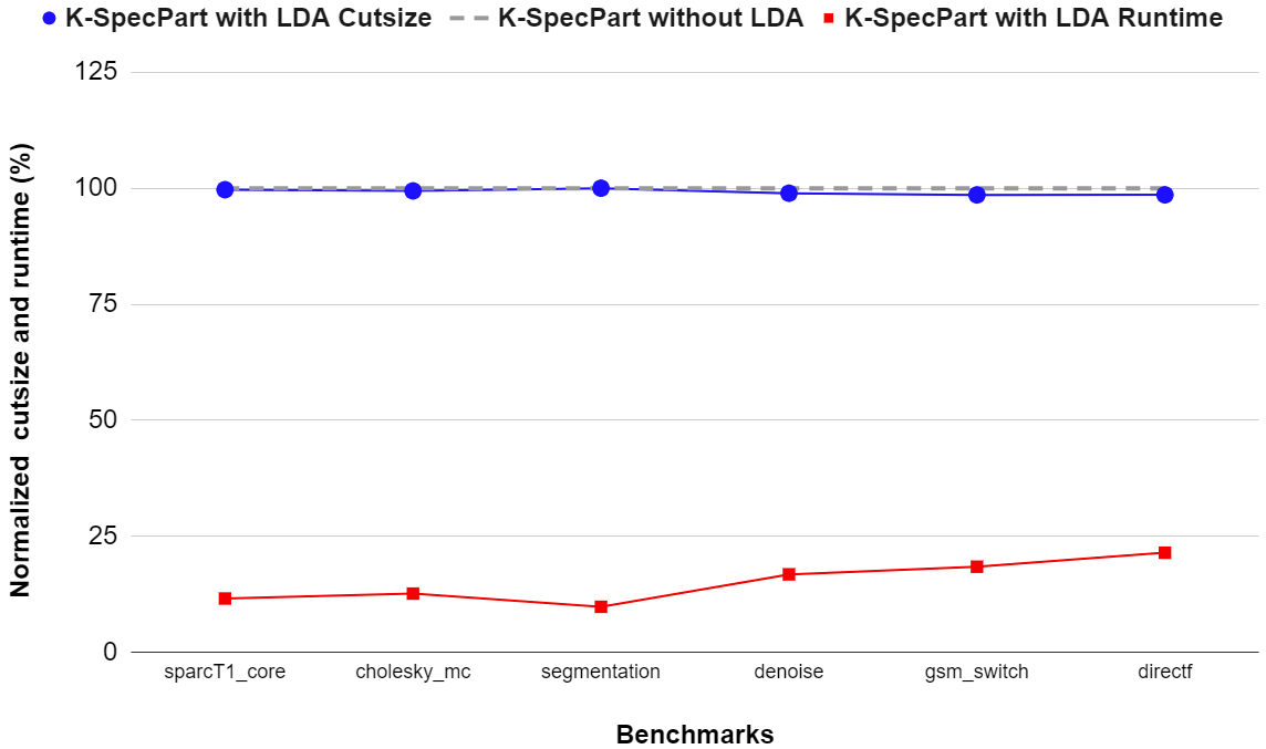
Figure 13: Comparison of cutsize and runtime of K-SpecPart with LDA and K-SpecPart without LDA, for $K=4$ and $\epsilon=2\%$.

VII-F VILE vs. Recursive Balanced Tree Partitioning

We additionally compare the “VILE” tree partitioning algorithm (Section V-C) with a balanced tree partitioning baseline, based on a recursive two-way cut distilling and partitioning of the tree, similar to Section V. During each level of recursive partitioning, we dynamically adjust the balance constraint to ensure that the final $K$-way partitioning solution satisfies the balance constraints (see Section II-A). In particular, while executing the $i^{th}$ ($1\leq i\leq K-1$) level bipartitioning, the balance constraints associated with the bipartitioning solution $S(V_{i0},V_{i1})$ are:

$$\begin{split}{\color[rgb]{0,0,0}(\frac{1}{K}-\epsilon)W\leq\sum_{v\in V_{i0}}{w_{v}}\leq(\frac{1}{K}+\epsilon)W}\end{split}$$ (9)

After obtaining the bipartitioning solution $S(V_{i0},V_{i1})$, we proceed with the $(i+1)^{th}$ level bipartitioning. A comparison of cutsize obtained with “VILE” tree partitioning and balanced tree partitioning is presented in Figure 14. The plots are normalized with respect to the cutsize obtained with balanced tree partitioning. We observe that “VILE” tree partitioning yields better cutsize (on average $2$% better) compared to balanced tree partitioning.

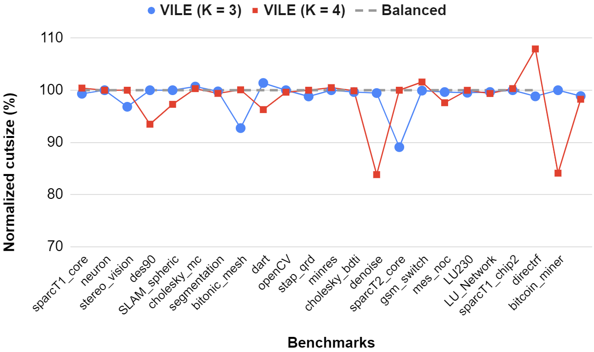
Figure 14: Comparison of “VILE” tree partitioning and balanced tree partitioning for $K=3,4$ and $\epsilon=2\%$.

VII-G Effect of Supervision in K-SpecPart

In order to show the effect of supervision in K-SpecPart, we run solution ensembling via cut overlay directly on candidate solutions, which are generated by running hMETIS multiple times with different random seeds. The flow is as follows. (i) We generate candidate solutions $\{S_{1},S_{2},...,S_{\psi}\}$ by running hMETIS $\psi$ times with different random seeds, and report the best cutsize Multi-start-hMETIS. Here $\psi$ is an integer parameter ranging from 1 to 20. (ii) We run solution ensembling via cut overlay directly on the best five solutions from $\{S_{1},S_{2},...,S_{\psi}\}$ and report the cutsize Solution-overlay-part. For each value of $\psi$, we run this flow $100$ times and report the average result in Figure 15. We observe that Solution-overlay-part is much better than Multi-start-hMETIS, and that K-SpecPart generates superior solutions in less runtime compared to Multi-start-hMETIS and Solution-overlay-part. This suggests that supervision is an important component of K-SpecPart.

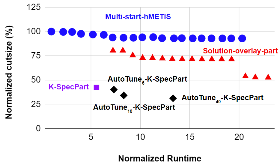
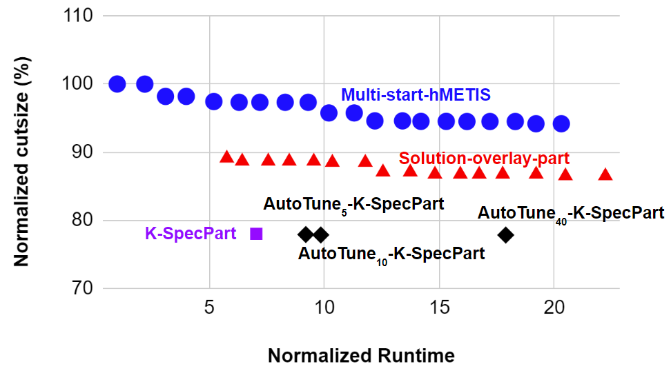
Figure 15: Cutsize versus runtime on gsm_switch, for $\epsilon=2\%$.
Top-to-bottom: $K=2,4$.

VII-H Solution Enhancement by Autotuning.

hMETIS has parameters whose settings may significantly impact the quality of generated partitioning solutions. We use Ray [51] to tune the following parameters of hMETIS: CType with possible values $\{1,2,3,4,5\}$, RType with possible values $\{1,2,3\}$, Vcycle with possible values $\{1,2,3\}$, and Reconst with possible values $\{0,1\}$. The search algorithm we use in Ray [51] is HyperOptSearch. We set the number of trials, i.e., total number of runs of hMETIS launched by Ray, to 5, 10 and 40. We set the number of threads to 10 to reduce the runtime (elapsed walltime). Here we normalize the cutsize and runtime to that of running hMETIS once with default random seed. Autotuning increases the runtime for hMETIS and computes a better hint $S_{init}$; it leads to a further $2\%$ cutsize improvement from K-SpecPart on gsm_switch for $K=2$ and $K=4$.

VIII Conclusion and Future Directions

We have proposed K-SpecPart, the first general supervised framework for hypergraph multi-way partitioning solution improvement. Our experimental results demonstrate the superior performance of K-SpecPart in comparison to traditional multilevel partitioners, while maintaining comparable runtimes for both bipartitioning and multi-way partitioning. The findings from SpecPart and K-SpecPart indicate that the partitioning problem may not be as comprehensively solved as previously believed, and that substantial advancements may yet remain to be discovered. K-SpecPart can be integrated with the internal levels of multilevel partitioners; producing improved solutions on each level may lead to further improved solutions. Furthermore, we believe that the cut-overlay clustering and LDA-based embedding generation hold independent interest and are amenable to machine learning techniques.

Acknowledgments. We thank Dr. Grigor Gasparyan for sharing his thoughts on K-SpecPart. This work was partially supported by NSF grants CCF-2112665, CCF-2039863 and CCF-1813374 and by DARPA HR0011-18-2-0032.

	Statistics		$K=2$			$K=3$			$K=4$
Benchmark	$|V|$	$|E|$	hMavg	KHPravg	K-SP	hMavg	KHPravg	K-SP	hMavg	KHPravg	K-SP
IBM01	$12752$	$14111$	$203.0$	$203.0$	$203$	$352.0$	$355.2$	$352$	$503.7$	$493.3$	$522$
IBM02	$19601$	$19584$	$331.5$	$350$	$333$	$339.4$	$357.2$	$339$	$676.5$	$701.3$	$706$
IBM03	$23136$	$27401$	$958.3$	$957.2$	$957$	$1544.2$	$1482.1$	$1480$	$1701.6$	$1693.9$	$1690$
IBM04	$27507$	$31970$	$581.3$	$581.3$	$580$	$1199.6$	$1203.6$	$1212$	$1669.4$	$1631.2$	$1626$
IBM05	$29347$	$28446$	$1728.6$	$1718.9$	$1716$	$2645.2$	$2642.4$	$2635$	$3031.2$	$2967.8$	$2946$
IBM06	$32498$	$34826$	$974.3$	$977.2$	$976$	$1306.7$	$1298.2$	$1305$	$1517.9$	$1515.2$	$1476$
IBM07	$45926$	$48117$	$910.3$	$913.2$	$935$	$1882.4$	$1873.4$	$1846$	$2201.4$	$2165.2$	$2154$
IBM08	$51309$	$50513$	$1141.2$	$1140.2$	$1140$	$2056.2$	$2011.9$	$2037$	$2401.5$	$2348.7$	$2328$
IBM09	$53395$	$60902$	$625.3$	$625.9$	$620$	$1404.1$	$1407.2$	$1384$	$1734.2$	$1675.1$	$1676$
IBM10	$69429$	$75196$	$1280.3$	$1327.7$	$1257$	$1911.8$	$1904.3$	$1880$	$2445.2$	$2372.9$	$2400$
IBM11	$70558$	$81454$	$1052.6$	$1066.5$	$1051$	$1808.5$	$1789.6$	$1843$	$2458.9$	$2465.8$	$2452$
IBM12	$71076$	$77240$	$1947.6$	$1961.9$	$1937$	$2817.3$	$2816.3$	$2791$	$3870.4$	$3894.2$	$3844$
IBM13	$84199$	$99666$	$844.3$	$848.4$	$832$	$1347.8$	$1345.3$	$1335$	$1913.2$	$1941.7$	$1904$
IBM14	$147605$	$152772$	$1875.1$	$1849.6$	$1850$	$2789.9$	$2607.5$	$2710$	$3401.4$	$3453.7$	$3475$
IBM15	$161570$	$186608$	$2817.2$	$2741.7$	$2741$	$4200.8$	$4114.2$	$4333$	$4870.7$	$4627.5$	$4720$
IBM16	$183484$	$190048$	$1925.6$	$2017.6$	$1921$	$3169.3$	$3107.3$	$3062$	$4045.2$	$4216.7$	$4060$
IBM17	$185495$	$189581$	$2364.5$	$2332.2$	$2307$	$4550.1$	$4305.1$	$4248$	$5634.6$	$5738.9$	$5583$
IBM18	$210613$	$201920$	$1531.6$	$1893.4$	$1523$	$2543.9$	$2487.6$	$2401$	$2949.4$	$2984.5$	$2918$

TABLE III: Comparison of hMETIS, KaHyPar and K-SpecPart on ISPD98 benchmarks with unit vertex weights for multi-way partitioning with number of blocks ($K$) = $2,3,4$ and imbalance factor ($\epsilon$) = $2\%$.

	Statistics		$K=2$			$K=3$			$K=4$
Benchmark	$|V|$	$|E|$	hMavg	KHPravg	K-SP	hMavg	KHPravg	K-SP	hMavg	KHPravg	K-SP
$IBM01_{w}$	$12752$	$14111$	$215.0$	$215.1$	$215$	$389.1$	$396.4$	$387$	$349.0$	$347.6$	$349$
$IBM02_{w}$	$19601$	$19584$	$324.6$	$349.4$	$296$	$340.9$	$354.3$	$334$	$548.4$	$565.7$	$524$
$IBM03_{w}$	$23136$	$27401$	$958.2$	$957.2$	$957$	$1249.8$	$1471.7$	$1230$	$1496.2$	$1473.1$	$1447$
$IBM04_{w}$	$27507$	$31970$	$584.7$	$582.4$	$529$	$899.6$	$805.4$	$797$	$1572.4$	$1532.4$	$1446$
$IBM05_{w}$	$29347$	$28446$	$1728.9$	$1716.9$	$1721$	$2640.1$	$2641.2$	$2642$	$3035.7$	$2960.5$	$3061$
$IBM06_{w}$	$32498$	$34826$	$969.3$	$979.7$	$845$	$997.2$	$998.1$	$963$	$1263.0$	$1314.8$	$1261$
$IBM07_{w}$	$45926$	$48117$	$812.3$	$824.5$	$803$	$1375.2$	$1367.1$	$1328$	$1902.4$	$1897.6$	$1824$
$IBM08_{w}$	$51309$	$50513$	$1142.4$	$1140.2$	$1182$	$1844.3$	$1794.2$	$1749$	$2407.9$	$2350.9$	$2268$
$IBM09_{w}$	$53395$	$60902$	$626.7$	$625.9$	$519$	$1407.2$	$1404.1$	$1334$	$1530.3$	$1675.9$	$1535$
$IBM10_{w}$	$69429$	$75196$	$1079.8$	$1329.1$	$1028$	$1576.0$	$1655.5$	$1560$	$2447.4$	$2328.4$	$2143$
$IBM11_{w}$	$70558$	$81454$	$845.2$	$863.9$	$763$	$1509.2$	$1501.3$	$1508$	$2069.5$	$2078.9$	$2068$
$IBM12_{w}$	$71076$	$77240$	$1947.3$	$1962.9$	$1967$	$2814.4$	$2816.5$	$3185$	$3859.7$	$3793.4$	$3613$
$IBM13_{w}$	$84199$	$99666$	$847.8$	$848.8$	$846$	$1639.1$	$1624.4$	$1636$	$1795.1$	$1840.2$	$1784$
$IBM14_{w}$	$147605$	$152772$	$1872.7$	$1855.2$	$1929$	$2814.5$	$2604.1$	$2780$	$3374.3$	$3251.2$	$3455$
$IBM15_{w}$	$161570$	$186608$	$2797.1$	$2741.3$	$2474$	$3864.5$	$3915.6$	$3836$	$4805.6$	$4633.3$	$4758$
$IBM16_{w}$	$183484$	$190048$	$1656.4$	$1689.2$	$1660$	$2942.3$	$2981.9$	$2742$	$3676.5$	$3892.1$	$3729$
$IBM17_{w}$	$185495$	$189581$	$2369.5$	$2334.5$	$2301$	$3589.3$	$3671.2$	$3580$	$5630.2$	$5729.1$	$5738$
$IBM18_{w}$	$210613$	$201920$	$1572.1$	$1930.3$	$1579$	$2503.3$	$2482.1$	$2836$	$2947.9$	$2979.6$	$3209$

TABLE IV: Comparison of hMETIS, KaHyPar and K-SpecPart on ISPD98 benchmarks with actual weights for multi-way partitioning with number of blocks ($K$) = $2,3,4$ and imbalance factor ($\epsilon$) = $2\%$.

	Statistics		$K=2$		$K=3$		$K=4$
Benchmark	$|V|$	$|E|$	hMavg	K-SP	hMavg	K-SP	hMavg	K-SP
sparcT1_core	$91976$	$92827$	$982.2$	$977$	$2187.9$	$1889$	$2532.3$	$2492$
neuron	$92290$	$125305$	$245.0$	$244$	$371.6$	$396$	$431.5$	$431$
stereo_vision	$94050$	$127085$	$171.0$	$169$	$332.7$	$336$	$440.2$	$475$
des90	$111221$	$139557$	$376.8$	$374$	$536.5$	$535$	$695.5$	$747$
SLAM_spheric	$113115$	$142408$	$1061.0$	$1061$	$2797.1$	$2720$	$3371.1$	$3241$
cholesky_mc	$113250$	$144948$	$282.0$	$282$	$886.5$	$864$	$982.8$	$984$
segmentation	$138295$	$179051$	$120.1$	$120$	$476.1$	$453$	$496.3$	$490$
bitonic_mesh	$192064$	$235328$	$585.2$	$584$	$895.0$	$895$	$1304.4$	$1311$
dart	$202354$	$223301$	$837.0$	$805$	$1189.9$	$1243$	$1429.9$	$1401$
openCV	$217453$	$284108$	$435.4$	$434$	$501.8$	$525$	$526.2$	$522$
stap_qrd	$240240$	$290123$	$377.4$	$464$	$501.2$	$497$	$714.5$	$674$
minres	$261359$	$320540$	$207.0$	$207$	$309.0$	$309$	$407.0$	$407$
cholesky_bdti	$266422$	$342688$	$1156.0$	$1136$	$1769.2$	$1755$	$1874.4$	$1865$
denoise	$275638$	$356848$	$496.9$	$418$	$952.8$	$915$	$1172.1$	$1001$
sparcT2_core	$300109$	$302663$	$1220.7$	$1188$	$2827.2$	$2249$	$3323.5$	$3558$
gsm_switch	$493260$	$507821$	$4235.3$	$1833$	$4148.6$	$3694$	$5169.2$	$4404$
mes_noc	$547544$	$577664$	$634.6$	$633$	$1164.3$	$1125$	$1314.7$	$1346$
LU230	$574372$	$669477$	$3333.3$	$3363$	$4549.5$	$4548$	$6325.3$	$6310$
LU_Network	$635456$	$726999$	$524.0$	$524$	$787.1$	$882$	$1495.6$	$1417$
sparcT1_chip2	$820886$	$821274$	$914.2$	$876$	$1453.4$	$1404$	$1609.8$	$1601$
directrf	$931275$	$1374742$	$602.6$	$515$	$728.2$	$762$	$1103.6$	$1092$
bitcoin_miner	$1089284$	$1448151$	$1514.1$	$1562$	$1944.8$	$1917$	$2605.4$	$2737$

TABLE V: Comparison of hMETIS and K-SpecPart on Titan23 benchmarks for multi-way partitioning with number of blocks ($K$) = $2,3,4$ and imbalance factor ($\epsilon$) = $2\%$.

References

- [1] M. Cucuringu, I. Koutis, S. Chawla, G. Miller and R. Peng, “Simple and scalable constrained clustering: a generalized spectral method”, Proc. International Conference on Artificial Intelligence and Statistics, 2016, pp. 445-454.
- [2] N. Alon, R. M. Karp, D. Peleg and D. West, “A graph-theoretic game and its application to the -server problem”, SIAM Journal on Computing 24(1) (1995), pp. 78-100.
- [3] J. B. Kruskal. “On the shortest spanning subtree of a graph and the traveling salesman problem”, Proc. American Mathematical Society 7(1) (1956), pp. 48-50.
- [4] C. J. Alpert, “The ISPD98 circuit benchmark suite”, Proc. ACM/IEEE International Symposium on Physical Design, 1998, pp. 80-85.
- [5] G. Karypis and V. Kumar, “A fast and high quality multilevel scheme for partitioning irregular graphs”, SIAM Journal on Scientific Computing 20(1) (1998), pp. 359-392.
- [6] G. Karypis, R. Aggarwal, V. Kumar and S. Shekhar, “Multilevel hypergraph partitioning: applications in VLSI domain”, IEEE Transactions on Very Large Scale Integration (VLSI) Systems 7(1) (1999), pp. 69-79.
- [7] M. Bender and M. Farach-Colton, “The LCA problem revisited”, Latin American Symposium On Theoretical Informatics pp. 88-94 (2000).
- [8] G. Karypis and V. Kumar, “hMETIS, a hypergraph partitioning package, version 1.5.3”, 1998. http://glaros.dtc.umn.edu/gkhome/fetch/sw/hMETIS/manual.pdf
- [9] K. E. Murray, S. Whitty, S. Liu, J. Luu and V. Betz, “Titan: Enabling large and complex benchmarks in academic CAD”, Proc. International Conference on Field Programmable Logic and Applications, 2013, pp. 1-8.
- [10] S. Balakrishnama and A. Ganapathiraju, “Linear discriminant analysis - a brief tutorial”, Institute for Signal and information Processing, 1998, pp. 1-8.
- [11] Ü. Çatalyürek and C. Aykanat, “PaToH (partitioning tool for hypergraphs)”, Boston, MA, Springer US, 2011.
- [12] J. Bezanson, A. Edelman, S. Karpinski and V. B. Shah, “Julia: a fresh approach to numerical computing”, SIAM Review 59(1) (2017), pp. 65-98.
- [13] C. M. Fiduccia and R. M. Mattheyses, “A linear-time heuristic for improving network partitions”, Proc. IEEE/ACM Design Automation Conference, 1982, pp. 175-181.
- [14] B. Ghojogh, F. Karray and M. Crowley, “Eigenvalue and generalized eigenvalue problems: tutorial”, arXiv:1903.11240, 2019.
- [15] R. Shaydulin, J. Chen and I. Safro, “Relaxation-based coarsening for multilevel hypergraph partitioning”, Multiscale Modeling & Simulation 17(1) (2019), pp. 482-506.
- [16] A. V. Knyazev, “Toward the optimal preconditioned eigensolver: locally optimal block preconditioned conjugate gradient method”, SIAM Journal on Scientific Computing 23(2) (2001), pp. 517-541.
- [17] T. Heuer, P. Sanders and S. Schlag, “Network flow-based refinement for multilevel hypergraph partitioning”, ACM Journal of Experimental Algorithmics 24(2) (2019), pp. 1-36.
- [18] D. Kucar, S. Areibi and A. Vannelli, “Hypergraph partitioning techniques”, Dynamics of Continuous, Discrete & Impulsive Systems. Series A: Mathematical Analysis 11(2) (2004), pp. 339-367.
- [19] R. Merris, “Laplacian matrices of graphs: a survey”, Linear Algebra and its Applications 197 (1994), pp. 143-176.
- [20] A. V. Knyazev, I. Lashuk, M. E. Argentati and E. Ovchinnikov, “Block locally optimal preconditioned eigenvalue xolvers (BLOPEX) in hypre and PETSc”, SIAM Journal on Scientific Computing 25(5) (2007), pp. 2224-2239.
- [21] I. Koutis, G. L. Miller and R. Peng, “Approaching optimality for solving SDD linear system”, SIAM Journal on Computing 43(1) (2014), pp. 337-354.
- [22] J. G. Sun and G. W. Stewart, Matrix Perturbation Theory, Boston, Elsevier Science, 1990.
- [23] I. Koutis, G. L. Miller and D. Tolliver, “Combinatorial preconditioners and multilevel solvers for problems in computer vision and image processing”, Computer Vision and Image Understanding 115(12) (2011), pp. 1638-1646.
- [24] A. E. Caldwell, A. B. Kahng and I. L. Markov, “Improved algorithms for hypergraph bipartitioning”, Proc. IEEE/ACM Design Automation Conference, 2000, pp. 661-666.
- [25] J. R. Lee, S. O. Gharan and L. Trevisan, “Multiway spectral partitioning and higher-order cheeger inequalities”, Journal of the ACM (61) (2014), pp. 1-30.
- [26] S. Mika, G. Rätsch, J. Weston, B. Schölkopf and K.-R. Müller, “Fisher discriminant analysis with kernels”, Proc. IEEE Signal Processing Society Workshop on Neural Networks for Signal Processing, 1999, pp. 41-48.
- [27] R. A. Fisher, “The use of multiple measurements in taxonomic problems”, Annals of Eugenics, 1936, pp. 179-188.
- [28] T. Heuer, “Engineering initial partitioning algorithms for direct k-way hypergraph partitioning”, Karlsruhe Institute of Technology, 2015.
- [29] S. Sebastian, H. Tobias, G. Lars, A. Yaroslav, S. Christian and S. Peter, “High-quality hypergraph partitioning”, ACM Journal of Experimental Algorithmics 27(1.9) (2023), pp. 1-39.
- [30] S. Schlag, V. Henne, T. Heuer, H. Meyerhenke, P. Sanders and C. Schulz, “k-way hypergraph partitioning via n-Level recursive bisection”, Proc. the Meeting on Algorithm Engineering and Experiments, 2016, pp. 53-67.
- [31] I. Bustany, A. B. Kahng, Y. Koutis, B. Pramanik and Z. Wang, “SpecPart: A supervised spectral framework for hypergraph partitioning solution improvement”, Proc. IEEE/ACM International Conference on Computer-Aided Design, 2022, pp. 1-9.
- [32] J. Y. Zien, M. D. F. Schlag and P. K. Chan, “Multilevel spectral hypergraph partitioning with arbitrary vertex sizes”, IEEE Transactions on Computer-Aided Design of Integrated Circuits and Systems 18(9) (1999), pp. 1389-1399.
- [33] L. Hagen and A. B. Kahng, “Fast spectral methods for ratio cut partitioning and clustering”, Proc. IEEE/ACM International Conference on Computer-Aided Design, 1991, pp. 10-13.
- [34] N. Rebagliati and A. Verri. “Spectral clustering with more than K eigenvectors”, Neurocomputing 74(9) (2011), pp. 1391-1401.
- [35] C. J. Alpert and A. B. Kahng, “Multiway partitioning via geometric embeddings, orderings, and dynamic programming”, IEEE Transactions on Computer-Aided Design of Integrated Circuits and Systems 14(11) (1995), pp. 1342-1358.
- [36] R. Horaud, “A short tutorial on graph Laplacians, Laplacian embedding, and spectral clustering”, 2009. https://csustan.csustan.edu/~tom/Clustering/GraphLaplacian-tutorial.pdf.
- [37] A. E. Caldwell, A. B. Kahng and I. L. Markov, “Improved algorithms for hypergraph bipartitioning”, Proc. of Asia and South Pacific Design Automation Conference, 2000, pp. 661-666.
- [38] F. R. K. Chung, “Spectral graph theory”, CBMS Regional Conference Series in Mathematics, 1997.
- [39] I. Koutis, G. Miller, and R. Peng, “A generalized Cheeger inequality”, Linear Algebra and its Applications, 2023, vol. 665, pp. 139-152
- [40] M. Kapralov and R. Panigrahy, “Spectral sparsification via random spanners”, Proc. Innovations in Theoretical Computer Science Conference, 2012, pp. 393-398.
- [41] S. Hoory and N. Linial, “Expander graphs and their applications”, Bulletin of the American Mathematical Society 43 (2006), pp. 439-561.
- [42] C. Ravishankar, D. Gaitonde and T. Bauer, “Placement strategies for 2.5D FPGA fabric architectures”, Proc. International Conference on Field Programmable Logic and Applications, 2018, pp. 16-164.
- [43] R. L. Graham and P. Hell, “On the history of the minimum spanning tree problem”, Annals of the History of Computing 7(1) (1985), pp. 43-57.
- [44] IBM ILOG CPLEX optimizer version 12.8.0, https://www.ibm.com/analytics/cplex-optimizer.
- [45] V. D. Blondel, J.-L. Guillaume, R. Lambiotte and E. Lefebvre, “Fast unfolding of communities in large networks”, Journal of Statistical Mechanics: Theory and Experiment 2008(10) (2008), pp. 10008.
- [46] E. G. Boman and B. Hendrickson, “Support theory for preconditioning”, SIAM Journal on Matrix Analysis and Applications 25(3) (2003), pp. 694-717.
- [47] C. J Alpert, A. B. Kahng and S.-Z. Yao, “Spectral partitioning with multiple eigenvectors”, Discrete Applied Mathematics 90(1) (1999), pp. 3-26.
- [48] https://github.com/kahypar/kahypar/blob/master/config/cut_rKaHyPar_sea20.ini
- [49] Partition solutions, scripts and K-SpecPart, https://github.com/TILOS-AI-Institute/HypergraphPartitioning.
- [50] TritonPart, an open-source partitioner, https://github.com/ABKGroup/TritonPart_OpenROAD
- [51] Ray, https://docs.ray.io/en/latest/index.html.
- [52] Y.-C. A. Wei and C.-K. Cheng, “Towards efficient hierarchical designs by ratio cut partitioning”, Proc. IEEE/ACM International Conference on Computer-Aided Design, 1989, pp. 298-301.
- [53] Google OR-Tools version 9.4, https://developers.google.com/optimization/
- [54] MultivariateStats.jl, https://github.com/JuliaStats/MultivariateStats.jl
- [55] Combinatorial multigrid solver, an implementation in Julia, https://github.com/bodhi91/CombinatorialMultigrid.jl