Distribution-Flexible Subset Quantization for Post-Quantizing Super-Resolution Networks

Abstract

This paper introduces Distribution-Flexible Subset Quantization (DFSQ), a post-training quantization method for super-resolution networks. Our motivation for developing DFSQ is based on the distinctive activation distributions of current super-resolution models, which exhibit significant variance across samples and channels. To address this issue, DFSQ conducts channel-wise normalization of the activations and applies distribution-flexible subset quantization (SQ), wherein the quantization points are selected from a universal set consisting of multi-word additive log-scale values. To expedite the selection of quantization points in SQ, we propose a fast quantization points selection strategy that uses $K$-means clustering to select the quantization points closest to the centroids. Compared to the common iterative exhaustive search algorithm, our strategy avoids the enumeration of all possible combinations in the universal set, reducing the time complexity from exponential to linear. Consequently, the constraint of time costs on the size of the universal set is greatly relaxed. Extensive evaluations of various super-resolution models show that DFSQ effectively retains performance even without fine-tuning. For example, when quantizing EDSR$\times$2 on the Urban benchmark, DFSQ achieves comparable performance to full-precision counterparts on 6- and 8-bit quantization, and incurs only a 0.1 dB PSNR drop on 4-bit quantization. Code is at https://github.com/zysxmu/DFSQ

1 Introduction

Image super-resolution (SR) is a fundamental low-level computer vision task that aims to restore high-resolution (HR) images from low-resolution input images (LR). Due to the remarkable success of deep neural networks (DNNs), DNNs-based SR models have become a de facto standard for SR task [28, 53, 4, 18, 52]. However, the astonished performance of recent SR models typically relies on increasing network size and computational cost, thereby limiting their applications, especially in resource-hungry devices such as smartphones. Therefore, compressing SR models has gained extensive attention from both academia and industries. Various network compressing techniques have been investigated to realize model deployment [29, 20, 11, 8].

Among these techniques, network quantization, which maps the full-precision weights and activations within networks to a low-bit format, harvests favorable interest from the SR community for its ability to reduce storage size and computation cost simultaneously [45, 13, 17, 50, 31, 24, 12, 54]. For example, [50, 31] quantize the SR models using binary quantization, and [24, 12, 54] quantize SR models to low-bit such as 2, 3, and 4-bit. Despite notable progress, current methods have to retrain quantized SR models on the premise of access to the entire training set, known as quantization-aware training (QAT). In real-world scenarios, however, acquiring original training data is sometimes prohibitive due to privacy, data transmission, and security issues. Besides, the heavy training and energy cost also prohibits its practical deployment. Post-training quantization (PTQ) methods, which perform quantization with only a small portion of the original training set, require no or a little retraining, by nature can be a potential way to solve the above problems [16, 7, 26, 36, 46]. However, current PTQ methods mostly are designed for high-level vision tasks, a direct extension of which to SR models is infeasible since low-level models comprise different structures [24, 54].

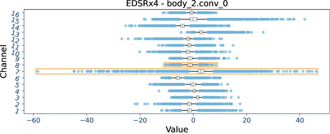
(a)

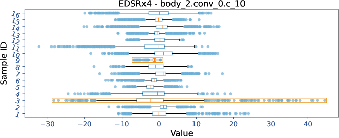
(b)

Figure 1: Variation of activation distributions of EDSR$\times$4 [28]. We show activation distributions of different channels given the same input (a), and of different inputs given the same channel (b). The orange box depicts the data with the maximum discrepancy.

More precisely, SR models usually remove all or most batch normalization (BN) layers since they reduce scale information within activations, which, as a wide consensus, is crucial to the performance of SR models [28, 53, 52, 9]. Unfortunately, the main obstacle of quantization also comes from the removal of BN since it leads to high activation variations such as considerable distribution discrepancy among different channels of the same sample and among the same channel of different samples. Taking Fig. LABEL:fig:insight-EDSRx4_channel as an example, for given a sample, the activation distributions among different channels vary a lot. At first, it can be seen the interquartile range (IQR) of channel_7 and channel_8 differs a lot. The IQR of the former is greater than 0 while the latter is less than 0. Second, the outlier distribution of channel_7 is far wide than that of channel_8, causing the activation range to differ by 5$\times$$\sim$6$\times$. In addition, as illustrated in Fig. LABEL:fig:insight-EDSRx4_sample, different samples present significant distribution discrepancies in channel_10. In particular, sample_3 manifests 10$\times$ more IQR than that of sample_9. Also, the activation of sample_3 ranges from -30 $\sim$ 48, while sample_9 only ranges from -8 $\sim$ 0. The high variance of activation across channels and samples makes it difficult to solve with current PTQ methods, which is also experimentally demonstrated in Sec. 4.3.

In this paper, we propose a Distribution-Flexible Subset Quantization (DFSQ) method to handle such highly variational activations. Specifically, considering the high variance among samples and channels, we first perform channel-wise normalization and then conduct distribution-flexible and hardware-friendly subset quantization (SQ) [38] to quantize the normalized activations. The normalization comprises two consecutive on-the-fly operations including subtracting the mean and dividing by the maximum absolute value for each channel of each sample. As a result, the range is normalized to -1 $\sim$ 1 whatever the input sample and the activation channel. Given the non-uniformity of normalized distribution, we suggest adopting the very recent subset quantization (SQ) [38], which aims to find the best quantization points from a universal set that consists of log-scale values. However, the search of quantization points in [38] involves an iterative exhaustive search algorithm that makes the time costs exponential w.r.t. the size of the universal set, resulting in prohibitive time overhead and limiting the size of the universal set. Therefore, we introduce a fast quantization points selection strategy to speed up the selection of quantization points in SQ. In particular, we perform bit-width related $K$-means clustering at first. Then, from a given universal set, we select the quantization points closest to $K$ centroids. Our strategy circumvents the enumeration of all possible combinations of quantization points in the universal set, and thereby reduces the time complexity from exponential to linear. Consequently, the limitation of time costs on the size of the universal set is greatly relaxed.

Extensive evaluations of two well-known SR models including EDSR [28] and RDN [53] on four benchmark datasets demonstrate the effectiveness of the proposed DFSQ. Notably, without any fine-tuning, DFSQ obtains comparable performance to the full-precision counterparts in high-bit cases such as 8 and 6-bit. For low-bit cases such as 4-bit, DFSQ is still able to greatly retain the performance. For example, on Urban100, DFSQ obtains 31.609 dB PSNR for EDSR$\times$2, only incurring less than 0.1 dB drops.

2 Related Work

2.1 Single Image Super Resolution

Along with the huge success of deep neural networks on many computer vision tasks, DNN-based SR models also obtain great performance increases and have dominated the field of image super-resolution. As a pioneer, Chao et al. [4] for the first time proposed an end-to-end SRCNN to learn the mapping relationship between LR and HR images. VDSR [18] further improves performance by increasing network depth. Afterward, skip-connection based blocks [22, 44] are extensively adopted by the subsequent studies [28, 53] to alleviate the gradient vanishing issue and retain image details. For better performance, researchers introduce many complex structures to construct SR models such as channel attention mechanism [52, 32], non-local attention [35, 34], and transformer-based block [27, 51]. With the increasing demand for the deployment of SR models on resource-limited devices, many studies aim to design lightweight network architectures. DRCN [19] and DRRN [42] both adopt the recursive structure to increase the depth of models while reducing the model size. Some studies design modules to substitute for the expensive up-sampling operation. FSRCNN [5] introduces a de-convolutional layer, and ESPCN [41] instead devises a sub-pixel convolution module. Many other studies utilize the efficient intermediate feature representation [21, 1, 15, 30] or network architecture search [37].

2.2 Quantized SR Models

Network quantization enjoys the merit of both reducing storage size and efficient low-bit operations and thereby harvesting ever-growing attention [45, 13, 17, 50, 31, 24, 12, 54]. Ma et al. [31] proposed binary quantization for the weights within SR models. Following them, BAM [50] and BTM [17] further binarize the activation of SR models. They introduce multiple feature map aggregations and skip connections to reduce the sharp performance drops caused by the binary activation. Other than binary quantization, many studies focus on performing low-bit quantization [45, 13, 24, 12, 54]. Li et al. [24] found unstable activation ranges and proposed a symmetric layer-wise linear quantizer, where a learnable clipping value is adopted to regulate the abnormal activation. Moreover, a knowledge distillation loss is devised to transfer structured knowledge of the full-precision model to the quantized model. Wang et al. [45] designed a fully-quantization method for SR models, in which the weight and activation within all layers are quantized with a symmetric layer-wise quantizer equipped with a learnable clipping value. Zhong et al. [54] observed that the activation exhibit highly asymmetric distributions and the range magnitude drastically varies with different input images. They introduced two learnable clipping values and a dynamic gate to adaptively adjust the clipping values. In [12], a dynamic bit-width adjustment network is introduced for different input patches that have various structure information.

3 Method

QAT usually trains the quantized network for many epochs, by accessing the entire training set, to gradually accommodate the quantization effect [6]. Differently, PTQ is confined to a small portion of the original training set, leading to a severe over-fitting issue [26]. Thus, the key to PTQ has drifted to fitting the data distribution. Below, we first demonstrate the obstacle in performing PTQ for SR models lies in the high variance activation distributions. Then, we introduce the subset quantization and a corresponding fast selection strategy.

3.1 Observations

It is a wide consensus that the removal batch normalization layer in SR models improves the quality of output HR images [28, 53, 52, 9]. Unfortunately, as discussed in many previous studies [13, 54, 24], the removal of the BN layer creates the obstacle for quantization since the resulting activations of high variance make low-bit networks hard to fit. In particular, the high-variance activations are two folds: 1) considerable distribution discrepancy in different channels for a given input sample; 2) considerable distribution discrepancy in different samples for a given channel.

Fig. 1 presents the example of activation distributions within EDSR$\times$4 [28]. Specifically, Fig. LABEL:fig:insight-EDSRx4_channel presents the activation distributions of different channels given the same sample. It can be seen that the distribution exhibits significant discrepancy. For example, the interquartile range of channel_7 is greater than 0 while channel_8 is less than 0. Moreover, the range of channel_7 is far wide than that of channel_8, resulting in a range difference by 5$\times$$\sim$6$\times$. Fig. LABEL:fig:insight-EDSRx4_sample presents the activation distribution of different input samples given the same channel. As it shows, given the same channel_10, extreme discrepancies between the distribution of different samples are revealed. Taking sample_3 and sample_9 as the example, the IQR of the former ranges from -6$\sim$1.5, while the latter ranges from -1.64$\sim$-0.8, almost 10$\times$ difference. Also, their range differs a lot. The activation of sample_3 ranges from -30$\sim$48, while sample_9 only ranges from -8$\sim$0, still resulting in a 10$\times$ difference. Therefore, the high-variance activation distribution is reflected by extreme discrepancy among different channels and different samples.

To handle such activation distributions, previous SR quantization methods rely on QAT to gradually adjust network weights to accommodate the quantization effect [6]. However, PTQ hardly succeeds in this manner since the availability of partial data easily causes over-fitting issue [26]. Moreover, the highly nonuniform distribution also makes the common linear uniform quantization adopted by current PTQ methods hard to fit the original distribution [25], which is also observed from our experimental results in Sec. 4.3. Therefore, the core is to find a suitable quantizer that can well fit the distribution as much as possible.

3.2 Distribution-Flexible Subset Quantization for Activation

3.2.1 Quantization Process

We denote a full-precision feature map as $X\in R^{B\times C\times H\times W}$, where $B,C,H,W$ respectively denote mini-batch size, channel number, height, and width of the feature maps. Considering that the activation distributions vary quite a lot across samples and channels, we choose to perform quantization for each channel of each sample, denoted as $X_{i,c}\in R^{H\times W}$, where $X_{i,c}$ denotes the $c$-th feature map (channel) of the $i$-th input sample. We suggest conducting normalization on-the-fly at first to scale the activation of $X_{i,c}$ as:

$$X^{n}_{i,c}=f_{n}(X_{i,c})=\frac{X_{i,c}-\mu_{i,c}}{\mathcal{M}_{i,c}-\mu_{i,c}},$$ (1)

where $\mu_{i,c}$ and $\mathcal{M}_{i,c}$ denote the mean value and maximum absolute value of $X_{i,c}$. The superscript “$n$” represents normalization.

After normalization, the activation is scaled to -1$\sim$1 whatever the input and channel are, thereby facilitating the following quantization:

$$X^{q}_{i,c}=Q(X^{n}_{i,c}),$$ (2)

$Q(\cdot)$ denotes the quantizer, which is elaborated in the next subsection. The superscript “$q$” denotes quantized results. Then, the de-quantized activation can be obtained by conducting de-normalization after getting $X^{q}_{i,c}$:

$$\bar{X}_{i,c}=f_{n}^{-1}(X^{q}_{i,c})=X^{q}_{i,c}\cdot\mathcal{M}_{i,c}+\mu_{i,c}.$$ (3)

Note that, the overhead of de-normalization can be reduced by quantizing $\mu_{i,c}$ and $\mathcal{M}_{i,c}$ to a low-bit format, which has already been studied in [3, 13].

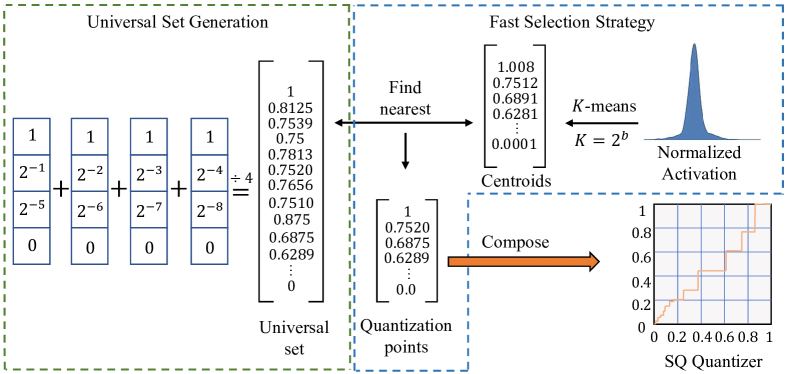
Figure 2: The framework of the proposed distribution-flexible subset quantization.

3.2.2 Subset Quantization

In this subsection, we elaborate on the aforementioned quantizer $Q(\cdot)$. Despite that the normalized activations conform to the same range across different channels and samples, they are still featured with high non-uniformity. Such erratic distributions are hard to be fitted by the common linear uniform quantization [25].

Therefore, we suggest the very recent distribution-flexible and hardware-friendly subset quantization (SQ) [38]. Specifically, SQ aims to find the best quantization points from a predefined universal set that usually consists of the additive of multi-word log-scale values [25, 39, 23]. Given a universal set $\Phi_{u}$, bit-width $b$, and an input value $x$, the quantizer $Q(\cdot)$ is defined as:

$$\begin{split}Q(x)&=\mathop{\arg\min}\limits_{p\in\Phi_{s}}|x-p|,\\ s.t.\quad\Phi_{s}&=\{p_{i}\in\Phi_{u}|i=1,\cdots,2^{b}\},\end{split}$$ (4)

where $\Phi_{s}$ is the set of selected quantization points. Therefore, the key steps of SQ are the universal set generation and the quantization points selection.

Universal Set Generation. The universal set $\Phi_{u}$ should contain adequate candidate values to represent any given input distribution [38]. The universal set used in our paper is presented in the left part of Fig. 2. Specifically, given four word sets, each of which contains four elements that are either zero or log-scale values. The universal set is obtained by averaging all possible combinations of the elements from each word set. For example, the value 0.8125 in the universal set is obtained by averaging the sum of 0 from the first word set, $2^{-2}$ from the second word set, and 1s from the third and fourth word sets. As a result, we can obtain a universal set that consists of many non-negative values. For distribution with negative values, it needs negative values. To do this, we add the negative values by changing the sign of non-negative values. For instance, if the value 0.8125 is present, its corresponding negative value, -0.8125, will also be added to the universal set. After duplicate removal, a total of 107 values are given as the universal set. Moreover, since each value of the universal set consists of four values that are either zero or $2^{k}$ and a division of 4, we can fuse the division of 4 into the elements of each word set. As a result, the multiplication between quantized activation and quantized weight only requires four shifters and one adder, which is hardware-friendly.

Quantization Points Selection. The common selection strategy of quantization points involves an iterative exhaustive search algorithm, where all possible combinations in the universal set are exhaustively checked to find out the one that minimizes the quantization loss. However, such a strategy incurs intolerable time costs as the size of the universal set increases. In particular, the number of all possible combinations is $C_{n}^{2^{b}}=\frac{n!}{2^{b}!(n-2^{b})!}$, where $b$ is the bit-width and $n$ is the size of the universal set. It can be seen the increase of combinations is an exponential growth w.r.t. the size of the universal set. For example, given the 4-bit case and the universal set defined above, the total number of combinations is $C_{107}^{2^{4}}=4.336\times 10^{18}$. Therefore, the size of the universal set is limited and a fast selection strategy is necessary.

3.2.3 Fast Selection Strategy

We then introduce a fast quantization points selection strategy to speed up the selection of quantization points in SQ. We are mainly inspired by the $K$-means algorithm which can be viewed as a solution for the quantization loss minimization problem with a given distribution and bit-width setting [49]. In particular, given $X^{n}_{i,c}$, we perform $K$-means clustering at first by setting $K=2^{b}$. To avoid the local optimum, in practice, we perform $K$-means by 3 times and select the results with the minimum sum of squared errors (SSE):

$$\begin{split}\Phi_{\mu}&=\mathop{\arg\min}\limits_{\Phi^{i}_{\mu}\in\{\Phi^{1}_{\mu},\Phi^{2}_{\mu},\Phi^{3}_{\mu}\}}\text{SSE}_{\Phi^{i}_{\mu}},\end{split}$$ (5)

where $\text{SSE}_{\Phi^{i}_{\mu}}=\sum_{x\in C^{i}_{j}}\|x-\mu^{i}_{j}\|^{2}$, $\Phi^{i}_{\mu}$ denotes the centroids set of $i$-th trial of $K$-means, $C^{i}_{j}$ denotes the $j$-th cluster of the $i$-th trial, and $\mu^{i}_{j}$ denotes the centroid of $C^{i}_{j}$. Then, from a given universal set, the quantization points set $\Phi_{s}$ is built by selecting these points closest to $K$ centroids of $\Phi_{\mu}$.

The time complexity of $K$-means is $\mathcal{O}(NTK)$, where $N=H\times W$ is the total number of elements in $X^{n}_{i,c}$, $T$ is the number of iterations in the clustering process, and $K=2^{b}$ [10]. Also, the selection of quantization points closest to $K$ centroids only requires $\mathcal{O}(|\Phi_{u}|2^{b})$. Note that the maximum bit-width $b$ generally is 8, which gives the $K=256$ at most. Thus, it is safe to say the time complexity of our fast selection strategy is linear. Note that, in practice, we can utilize the multiprocessing mechanism to process the feature map of each channel in parallel, enabling more efficient use of computing resources.

In summary, the time complexity of our strategy linearly depends on the $N,K,T$ and the size of the universal set. Compared with the previous iterative exhaustive search algorithm, the time complexity is reduced from exponential to linear. The cumbersome drudgery of enumerating all possible combinations is avoided and therefore the limitation of time costs on the size of the universal set is greatly relaxed.

3.3 Weight Quantization

For weight quantization, we adopt kernel-wise linear uniform quantization. Given the weight $W\in R^{C_{out}\times C_{in}\times K\times K}$, where $C_{out},C_{in},K$ denote output channel number, input channel number, and kernel size, respectively. For a kernel $W_{k}$, the quantizer is defined as:

$$W^{q}_{k}=round(\frac{W}{s})+Z,\quad s=\frac{u_{w}-l_{w}}{2^{b}-1},\quad Z=round(\frac{-l_{w}}{s}),$$ (6)

where $b,l_{w},u_{w},s,Z$ denote bit-width, weight minimum, weight maximum, step size, and zero-point integer corresponding to the full-precision $0$ respectively. The de-quantized value is obtained by:

$$\bar{W}_{k}=s\cdot(W^{q}_{k}-Z).$$ (7)

4 Experimentation

4.1 Implementation Details

The quantized SR models include two classical EDSR [28] and RDN [53]. For each SR model, we evaluate two upscaling factors of $\times$2 and $\times$4 and perform 8-, 6-, 4-, and 3-bit quantization, respectively. The calibration dataset contains 32 images random sampled from the training set of DIV2K [43]. The models are tested on four standard benchmarks including Set5 [2], Set14 [22], BSD100 [33] and Urban100 [14]. For the compared method, we adopt the Min-Max linear uniform quantization and two recent optimization-based methods including BRECQ [26] and QDROP [48]. We report the PSNR and SSIM [47] over the Y channel as the metrics.

The full-precision models and compared methods are implemented based on the official open-source code. Following [24, 54], we quantize both weights and activations of the high-level feature extraction module of the quantized models. The low-level feature extraction and reconstruction modules retain the full-precision. All experiments are implemented with PyTorch [40]

Table 1: Effect of different components in our paper. “Cha.”: channel-wise activation quantization. “Norm.”: normalization. The results are obtained by quantizing EDSR$\times$4 to 4-bit and the PSNR/SSIM is reported as the metrics.

Components		Results
Cha.	Norm.	Set5 [2]	Set14 [22]	BSD100 [33]	Urban100 [14]
		-	-	-	-
✓		-	-	-	-
	✓	31.543/0.8790	28.262/0.7675	27.358/0.7247	25.601/0.7586
✓	✓	31.689/0.8835	28.339/0.7728	27.409/0.7295	25.723/0.7707

Table 2: PSNR/SSIM results of the compared baseline and our DFSQ in quantizing EDSR [28] of scale $\times$2 and $\times$4. Results of the full-precision model are presented below the dataset name.

Model	Dataset	Bit	BRECQ [26]	QDROP [48]	Min-Max	DFSQ(Ours)
EDSR $\times$2	Set5 [2] 37.931/0.9604	8	37.921/0.9603	37.926/0.9603	37.926/0.9603	37.928/0.9603
		6	37.865/0.9597	37.882/0.9598	37.905/0.9601	37.927/0.9603
		4	37.499/0.9564	37.370/0.9572	37.497/0.9559	37.832/0.9599
		3	36.845/0.9500	36.603/0.9526	36.199/0.9383	37.382/0.9567
	Set14 [22] 33.459/0.9164	8	33.457/0.9163	33.457/0.9163	33.451/0.9164	33.459/0.9164
		6	33.419/0.9157	33.398/0.9159	33.436/0.9161	33.455/0.9164
		4	33.138/0.9123	32.947/0.9123	33.229/0.9122	33.399/0.9159
		3	32.714/0.9054	32.459/0.9074	32.477/0.8955	33.068/0.9113
	BSD100 [33] 32.102/0.8987	8	32.098/0.8986	32.099/0.8986	32.100/0.8987	32.101/0.8987
		6	32.066/0.8979	32.060/0.8980	32.089/0.8984	32.099/0.8986
		4	31.829/0.8939	31.710/0.8939	31.911/0.8941	32.060/0.8981
		3	31.475/0.8866	31.324/0.8885	31.263/0.8764	31.824/0.8939
	Urban100 [14] 31.709/0.9248	8	31.698/0.9246	31.683/0.9245	31.663/0.9245	31.707/0.9247
		6	31.588/0.9235	31.463/0.9228	31.642/0.9241	31.698/0.9246
		4	30.874/0.9158	30.265/0.9111	31.367/0.9188	31.609/0.9236
		3	30.106/0.9041	29.407/0.8989	30.395/0.8977	30.972/0.9137
EDSR $\times$4	Set5 [2] 32.095/0.8938	8	32.088/0.8935	32.089/0.8936	32.087/0.8936	32.090/0.8937
		6	32.018/0.8909	31.996/0.8911	32.056/0.8925	32.079/0.8933
		4	31.287/0.8722	31.103/0.8715	31.364/0.8687	31.755/0.8855
		3	30.164/0.8342	30.286/0.8478	29.150/0.7580	30.757/0.8489
	Set14 [22] 28.576/0.7813	8	28.566/0.7809	28.566/0.7810	28.566/0.7809	28.568/0.7810
		6	28.516/0.7788	28.501/0.7788	28.549/0.7801	28.560/0.7807
		4	28.080/0.7635	27.922/0.7634	28.159/0.7617	28.397/0.7749
		3	27.396/0.7330	27.392/0.7446	26.723/0.6681	27.732/0.7431
	BSD100 [33] 27.562/0.7355	8	27.557/0.7352	27.557/0.7352	27.555/0.7351	27.558/0.7354
		6	27.507/0.7326	27.509/0.7330	27.547/0.7344	27.555/0.7351
		4	27.198/0.7184	27.153/0.7197	27.255/0.7168	27.430/0.7307
		3	26.717/0.6903	26.811/0.7032	26.117/0.6253	27.044/0.7074
	Urban100 [14] 26.035/0.7848	8	26.018/0.7843	26.002/0.7841	26.014/0.7844	26.025/0.7845
		6	25.907/0.7801	25.849/0.7791	25.997/0.7831	26.020/0.7840
		4	25.291/0.7543	25.044/0.7485	25.588/0.7595	25.769/0.7736
		3	24.560/0.7124	24.460/0.7188	24.287/0.6520	24.987/0.7249

Table 3: PSNR/SSIM results of the compared baseline and our DFSQ in quantizing RDN [28] of scale $\times$2 and $\times$4.

Model	Dataset	Bit	BRECQ [26]	QDROP [48]	Min-Max	DFSQ(Ours)
RDN $\times$2	Set5 [2] 38.053/0.9607	8	38.019/0.9603	38.020/0.9604	38.049/0.9606	38.053/0.9607
		6	37.884/0.9588	37.873/0.9591	37.975/0.9599	38.042/0.9606
		4	37.143/0.9538	37.050/0.9540	37.172/0.9544	37.786/0.9593
		3	36.135/0.9469	36.000/0.9469	35.872/0.9464	37.125/0.9559
	Set14 [22] 33.594/0.9174	8	33.576/0.9172	33.566/0.9172	33.560/0.9175	33.589/0.9174
		6	33.464/0.9158	33.417/0.9160	33.530/0.9168	33.585/0.9173
		4	32.949/0.9106	32.825/0.9101	33.136/0.9108	33.373/0.9154
		3	32.322/0.9032	32.158/0.9012	32.297/0.8996	32.896/0.9105
	BSD100 [33] 32.197/0.8998	8	32.185/0.8995	32.187/0.8996	32.193/0.8998	32.195/0.8998
		6	32.120/0.8982	32.115/0.8985	32.167/0.8991	32.184/0.8996
		4	31.761/0.8932	31.689/0.8934	31.818/0.8913	32.043/0.8973
		3	31.281/0.8859	31.191/0.8851	31.133/0.8782	31.675/0.8919
	Urban100 [14] 32.125/0.9286	8	32.088/0.9282	32.051/0.9282	32.014/0.9281	32.115/0.9285
		6	31.827/0.9260	31.713/0.9257	31.975/0.9274	32.079/0.9281
		4	30.681/0.9150	30.367/0.9128	31.418/0.9193	31.594/0.9217
		3	29.532/0.8989	29.214/0.8930	30.086/0.8998	30.504/0.9080
RDN $\times$4	Set5 [2] 32.244/0.8959	8	32.233/0.8953	32.230/0.8954	32.238/0.8956	32.244/0.8959
		6	32.148/0.8929	32.141/0.8930	32.191/0.8941	32.228/0.8955
		4	31.498/0.8801	31.341/0.8794	31.619/0.8798	31.932/0.8895
		3	30.509/0.8586	30.455/0.8602	30.430/0.8546	31.077/0.8718
	Set14 [22] 28.669/0.7838	8	28.657/0.7834	28.650/0.7834	28.642/0.7835	28.663/0.7837
		6	28.582/0.7811	28.563/0.7812	28.616/0.7822	28.653/0.7834
		4	28.139/0.7701	28.032/0.7696	28.303/0.7701	28.471/0.7774
		3	27.516/0.7528	27.468/0.7537	27.621/0.7478	27.941/0.7616
	BSD100 [33] 27.627/0.7379	8	27.620/0.7375	27.621/0.7376	27.618/0.7377	27.625/0.7378
		6	27.575/0.7354	27.572/0.7360	27.597/0.7365	27.616/0.7375
		4	27.305/0.7261	27.249/0.7268	27.367/0.7245	27.504/0.7326
		3	26.918/0.7123	26.916/0.7143	26.889/0.7037	27.158/0.7195
	Urban100 [14] 26.293/0.7924	8	26.262/0.7916	26.245/0.7915	26.182/0.7904	26.292/0.7924
		6	26.116/0.7875	26.061/0.7870	26.157/0.7891	26.266/0.7914
		4	25.448/0.7662	25.292/0.7636	25.789/0.7720	25.960/0.7780
		3	24.700/0.7351	24.590/0.7331	24.921/0.7340	25.156/0.7442

4.2 Ablation Study

The ablation study of different components in our paper is presented in Tab. 1. When utilizing both channel-wise activation and normalization, our DFSQ presents the best results. As shown in the results of the first row and the second row, the quantized model suffers from collapse if normalization is not applied, indicating the importance of normalization for the subset quantization. The third row provides the results of not applying channel-wise quantization for activation, i.e., layer-wise activation quantization. It can be seen that channel-wise activation brings performance improvements. In particular, on Urban100, the quantized model presents 25.601 dB PSNR if not using channel-wise activation, while it is 25.732 dB PSNR if using channel-wise activation, demonstrating the effectiveness of handling each channel independently.

4.3 Quantitative Results

In this subsection, we provide quantitative results of EDSR and RDN across various bit-widths. The qualitative results are presented in the supplementary materials.

4.3.1 EDSR

Tab. 2 presents the quantitative results of EDSR$\times$2 and EDSR$\times$4. It can be seen that our DFSQ obtains the best performance across different datasets and bit-widths. Specifically, when performing high-bit PTQ, such as 8- and 6-bit quantization, our DFSQ achieves comparable performance to the full-precision counterpart. For instance, on 8- and 6-bit EDSR$\times$2, DFSQ obtains 32.101 dB and 32.099 dB PSNR on BSD100, which only gives a drop of 0.001 dB and 0.003 dB compared with the full-precision model, respectively. Also, results of 8- and 6-bit EDSR$\times$4 on BSD100 demonstrate that DFSQ only incurs 0.004 dB and 0.007 dB PSNR drop, respectively. It is worth emphasizing that the performance superiority of DFSQ exhibits as the bit-width goes down. Taking results of EDSR$\times$2 on Urban100 as the example, compared with the best result from other competitors, DFSQ obtains gains of 0.009 dB PSNR. For 6-, 4-, and 3-bit cases, DFSQ brings improvement of 0.056 dB, 0.242 dB, and 0.532 dB PSNR, respectively. Results of EDSR$\times$4 also provide a similar conclusion. For example, on Urban100, our DFSQ improves the PSNR by 0.007 dB, 0.023 dB, 0.181 dB, and 0.427 dB for For 8-, 6-, 4-, and 3-bit cases, respectively. Moreover, despite fine-tuning the weights, optimization-based BRECQ and QDROP exhibit lower performance than the simple Min-Max at most bit-widths, indicating they suffer from the over-fitting issue. In contrast, our DFSQ does not need any fine-tuning, and still achieves stable superior performance across all bit-widths.

4.4 RDN

Quantitative results of RDN are presented in Tab. 3. As can be seen, DFSQ obtains the best performance over different bit-widths and datasets. For the high-bit cases, DFSQ provides comparable performance to the full-precision model. For example, on 8- and 6-bit RDN$\times$2, DFSQ obtains 32.915 dB and 32.184 dB PSNR on BSD100, corresponding to 0.002 dB and 0.013 dB drop. While on 8- and 6-bit RDN$\times$4, DFSQ only incurs decreases of 0.002 dB and 0.011 dB on BSD100, respectively. Also, the performance advantage of our DFSQ becomes increasingly apparent as the bit-widths decrease. In particular, for RDN$\times$2 on Urban100, DFSQ improves the PSNR by 0.027 dB, 0.104 dB, 0.176 dB, and 0.418 dB on 8-, 6-, 4-, and 3-bit, respectively. While for RDN$\times$4 on Urban100, our DFSQ obtains performance gains by 0.03 dB, 0.109 dB, 0.171 dB, and 0.235 dB PSNR on 8-, 6-, 4-, and 3-bit, respectively. Moreover, it can be observed that the optimization-based methods do not even give higher results than min-max methods for 6- and 4-bit cases, indicating the existence of the over-fitting issue.

5 Discussion

Despite our DFSQ makes big progress, it involves an expensive channel-wise normalization before quantization. Thus, reducing the overhead incurred by normalization is worth to be further explored. For example, the de-normalization can be realized in low-bit as in [3, 13]. In addition, although optimization-based methods exhibit satisfactory performance on high-level tasks, they suffer from the over-fit issue as shown in Sec. 4.3. Therefore, a specialized optimization-based PTQ for SR could be a valuable direction.

6 Conclusion

In this paper, we present a novel quantization method, termed Distribution-Flexible Subset Quantization (DFSQ) for post-training quantization on super-resolution networks. We discover that the activation distribution of SR models exhibits significant variance between samples and channels. Correspondingly, our DFSQ suggests conducting a channel-wise normalization for activation at first, then applying the hardware-friendly and distribution-flexible subset quantization, in which the quantization points are selected from a universal set consisting of multi-word additive log-scale values. To select quantization points efficiently, we propose a fast quantization points selection strategy with linear time complexity. We perform $K$-means clustering to identify the closest quantization points to centroids from the universal set. Our DFSQ shows its superiority over many competitors on different quantized SR models across various bit-widths and benchmarks, especially when performing ultra-low precision quantization.

Acknowledgements. This work was supported by National Key R&D Program of China (No.2022ZD0118202), the National Science Fund for Distinguished Young Scholars (No.62025603), the National Natural Science Foundation of China (No. U21B2037, No. U22B2051, No. 62176222, No. 62176223, No. 62176226, No. 62072386, No. 62072387, No. 62072389, No. 62002305 and No. 62272401), and the Natural Science Foundation of Fujian Province of China (No.2021J01002, No.2022J06001).

Appendix

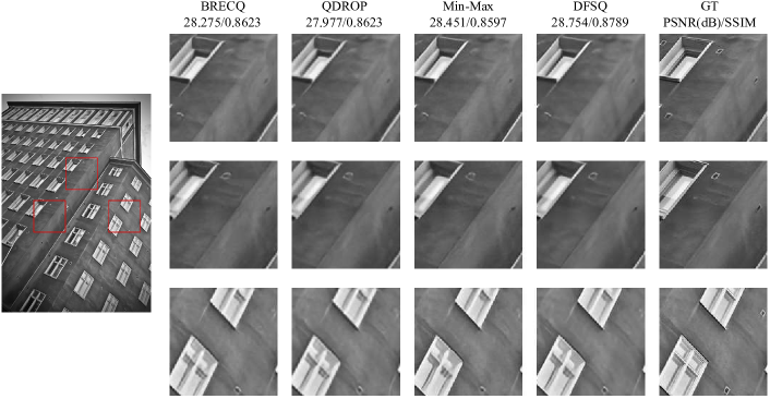
(a)

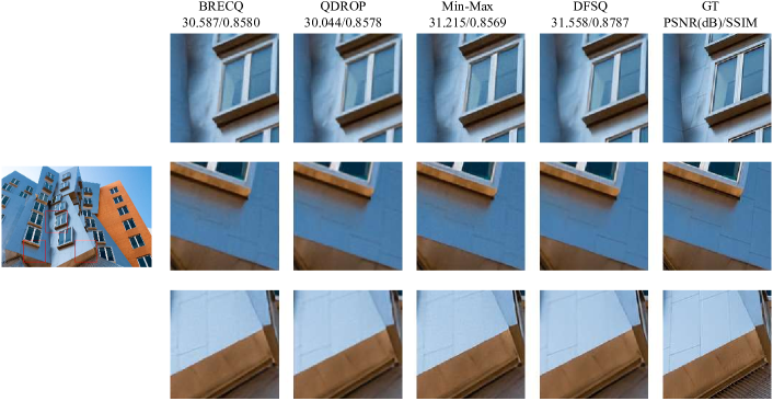
(b)

Figure 3: Illustration of the qualitative results of 4-bit EDSR$\times$4.

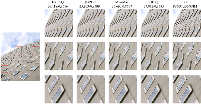
(a)

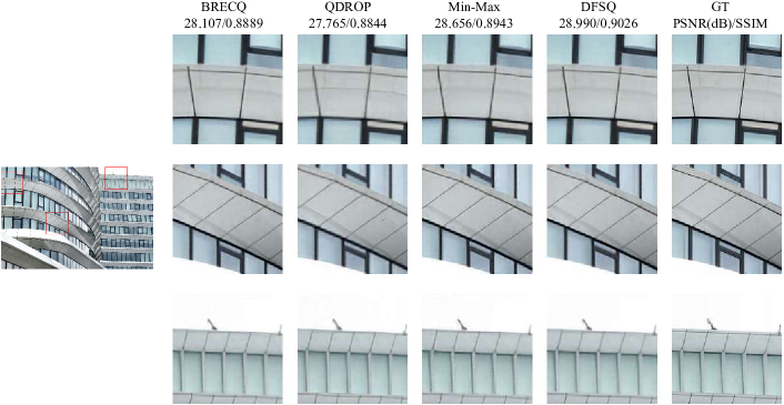
(b)

Figure 4: Illustration of the qualitative results of 4-bit RDN$\times$4.

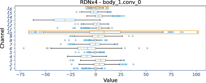
(a)

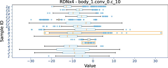
(b)

Figure 5: Illustration of high variance activation within RDN$\times$4. (a) and (b) present the activation distribution of different channels given the same sample and of different samples given the same channel, respectively. The orange box depicts the data with the maximum discrepancy.

Appendix A Qualitative Results

Fig. 3 and Fig. 4 exhibit the qualitative results of the 4-bit EDSR$\times$4 and 4-bit RDN$\times$4, respectively. The reported PSNR/SSIM are measured by the displayed image. It can be seen that our method obtains the best visualization results compared with other methods, which demonstrates the superiority of our DFSQ.

Appendix B More Illustrations

In this section, we provide more illustrations of the activation within SR models. Fig. 5 provides the activation distribution of RDN$\times$4. It can be seen that the distribution of activation varies a lot across different channels and samples. For example, as shown in Fig. LABEL:fig:insight-RDNx4_channel, the range of channel_16 is -10 to 10, while the range of channel_16 is -65 to 100. Distributions of the same sample but different channels shown in Fig. LABEL:fig:insight-RDNx4_sample also exhibit a large variance. Specifically, the range of channel_5 is -6 to 2, while the range of channel_8 is -23 to 32.

Table 4: Universal set designing.

Settings	Setting1	Setting2	Setting3	Setting4
Word Sets	{1, $2^{-1},2^{-3},0$}, {1, $2^{-2},2^{-4},0$}.	{1, $2^{-1},2^{-3},0$}, {1, $2^{-2},2^{-4},0$}, {1, $2^{-3},2^{-5},0$}.	{1, $2^{-1},2^{-5},0$}, {1, $2^{-2},2^{-6},0$}, {1, $2^{-3},2^{-7},0$}, {1, $2^{-4},2^{-8},0$}.	{1, $2^{-1},2^{-6},0$}, {1, $2^{-2},2^{-7},0$}, {1, $2^{-3},2^{-8},0$}, {1, $2^{-4},2^{-9},0$}, {1, $2^{-5},2^{-10},0$}.

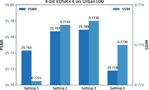
Figure 6: Results of 4-bit EDSR$\times$4 on Urban100 with different universal set settings.

Appendix C Ablation of Universal Set

In this section, we provide the experimental results of different universal sets by adjusting the number of word sets. In particular, we fix the size of each word set and vary the number of word sets to construct different universal sets. Four settings including 2$\times$4, 3$\times$4, 4$\times$4, and 5$\times$4 are provided as presented in Tab. 5. Note that the 4$\times$4 setting is the one we used in our main paper. The performance comparison is presented in Fig. 6. It can be seen that by increasing the number of word sets from 2 to 3 (2$\times$4 vs. 3$\times$4), the PSNR is improved by 0.34 dB. When the number of word sets is further increased to 4, the PSNR is improved by 0.002 dB. While at the 5$\times$4 setting, the PSNR drops by 0.051 dB, indicating the over-fitting issue. Thus, we choose to use the 4$\times$4 setting since the division of 4 can be achieved by performing bit shift operations on the elements of each word set.

References

- [1] Namhyuk Ahn, Byungkon Kang, and Kyung-Ah Sohn. Fast, accurate, and lightweight super-resolution with cascading residual network. In Proceedings of the European Conference on Computer Vision (ECCV), pages 252–268, 2018.
- [2] Marco Bevilacqua, Aline Roumy, Christine Guillemot, and Marie-Line Alberi Morel. Low-complexity single-image super-resolution based on nonnegative neighbor embedding. In British Machine Vision Conference (BMVC), 2012.
- [3] Steve Dai, Rangha Venkatesan, Mark Ren, Brian Zimmer, William Dally, and Brucek Khailany. Vs-quant: Per-vector scaled quantization for accurate low-precision neural network inference. Proceedings of Machine Learning and Systems (MLSys), 3:873–884, 2021.
- [4] Chao Dong, Chen Change Loy, Kaiming He, and Xiaoou Tang. Learning a deep convolutional network for image super-resolution. In Proceedings of the European Conference on Computer Vision (ECCV), pages 184–199, 2014.
- [5] Chao Dong, Chen Change Loy, and Xiaoou Tang. Accelerating the super-resolution convolutional neural network. In Proceedings of the European Conference on Computer Vision (ECCV), pages 391–407, 2016.
- [6] Steven K. Esser, Jeffrey L. McKinstry, Deepika Bablani, Rathinakumar Appuswamy, and Dharmendra S. Modha. Learned step size quantization. In Proceedings of the International Conference on Learning Representations (ICLR), 2020.
- [7] Jun Fang, Ali Shafiee, Hamzah Abdel-Aziz, David Thorsley, Georgios Georgiadis, and Joseph H Hassoun. Post-training piecewise linear quantization for deep neural networks. In Proceedings of the European Conference on Computer Vision (ECCV), pages 69–86. Springer, 2020.
- [8] Song Han, Jeff Pool, John Tran, William J Dally, et al. Learning both weights and connections for efficient neural network. In Proceedings of the Advances in Neural Information Processing Systems (NeurIPS), pages 1135–1143, 2015.
- [9] Muhammad Haris, Gregory Shakhnarovich, and Norimichi Ukita. Deep back-projection networks for super-resolution. In Proceedings of the IEEE/CVF Conference on Computer Vision and Pattern Recognition (CVPR), pages 1664–1673, 2018.
- [10] John A Hartigan and Manchek A Wong. Algorithm as 136: A k-means clustering algorithm. Journal of the royal statistical society. series c (applied statistics), 28(1):100–108, 1979.
- [11] Geoffrey Hinton, Oriol Vinyals, and Jeff Dean. Distilling the knowledge in a neural network. arXiv preprint arXiv:1503.02531, 2015.
- [12] Cheeun Hong, Sungyong Baik, Heewon Kim, Seungjun Nah, and Kyoung Mu Lee. Cadyq: Content-aware dynamic quantization for image super-resolution. In Proceedings of the European Conference on Computer Vision (ECCV), pages 367–383. Springer, 2022.
- [13] Cheeun Hong, Heewon Kim, Sungyong Baik, Junghun Oh, and Kyoung Mu Lee. Daq: Channel-wise distribution-aware quantization for deep image super-resolution networks. In Proceedings of the IEEE/CVF Winter Conference on Applications of Computer Vision (WACV), pages 2675–2684, 2022.
- [14] Jia-Bin Huang, Abhishek Singh, and Narendra Ahuja. Single image super-resolution from transformed self-exemplars. In Proceedings of the IEEE/CVF Conference on Computer Vision and Pattern Recognition (CVPR), pages 5197–5206, 2015.
- [15] Zheng Hui, Xinbo Gao, Yunchu Yang, and Xiumei Wang. Lightweight image super-resolution with information multi-distillation network. In Proceedings of the 27th acm international conference on multimedia (ACM MM), pages 2024–2032, 2019.
- [16] Yongkweon Jeon, Chungman Lee, Eulrang Cho, and Yeonju Ro. Mr.biq: Post-training non-uniform quantization based on minimizing the reconstruction error. In Proceedings of the IEEE/CVF Conference on Computer Vision and Pattern Recognition (CVPR), pages 12319–12328, 2022.
- [17] Xinrui Jiang, Nannan Wang, Jingwei Xin, Keyu Li, Xi Yang, and Xinbo Gao. Training binary neural network without batch normalization for image super-resolution. In Proceedings of the AAAI Conference on Artificial Intelligence (AAAI), pages 1700–1707, 2021.
- [18] Jiwon Kim, Jung Kwon Lee, and Kyoung Mu Lee. Accurate image super-resolution using very deep convolutional networks. In Proceedings of the IEEE/CVF Conference on Computer Vision and Pattern Recognition (CVPR), pages 1646–1654, 2016.
- [19] Jiwon Kim, Jung Kwon Lee, and Kyoung Mu Lee. Deeply-recursive convolutional network for image super-resolution. In Proceedings of the IEEE/CVF Conference on Computer Vision and Pattern Recognition (CVPR), pages 1637–1645, 2016.
- [20] Raghuraman Krishnamoorthi. Quantizing deep convolutional networks for efficient inference: A whitepaper. arXiv preprint arXiv:1806.08342, 2018.
- [21] Wei-Sheng Lai, Jia-Bin Huang, Narendra Ahuja, and Ming-Hsuan Yang. Deep laplacian pyramid networks for fast and accurate super-resolution. In Proceedings of the IEEE/CVF Conference on Computer Vision and Pattern Recognition (CVPR), pages 624–632, 2017.
- [22] Christian Ledig, Lucas Theis, Ferenc Huszár, Jose Caballero, Andrew Cunningham, Alejandro Acosta, Andrew Aitken, Alykhan Tejani, Johannes Totz, Zehan Wang, et al. Photo-realistic single image super-resolution using a generative adversarial network. In Proceedings of the IEEE/CVF Conference on Computer Vision and Pattern Recognition (CVPR), pages 4681–4690, 2017.
- [23] Sugil Lee, Hyeonuk Sim, Jooyeon Choi, and Jongeun Lee. Successive log quantization for cost-efficient neural networks using stochastic computing. In ACM/IEEE Design Automation Conference (DAC), pages 1–6, 2019.
- [24] Huixia Li, Chenqian Yan, Shaohui Lin, Xiawu Zheng, Baochang Zhang, Fan Yang, and Rongrong Ji. Pams: Quantized super-resolution via parameterized max scale. In Proceedings of the European Conference on Computer Vision (ECCV), pages 564–580, 2020.
- [25] Yuhang Li, Xin Dong, and Wei Wang. Additive powers-of-two quantization: An efficient non-uniform discretization for neural networks. In Proceedings of the International Conference on Learning Representations (ICLR), 2020.
- [26] Yuhang Li, Ruihao Gong, Xu Tan, Yang Yang, Peng Hu, Qi Zhang, Fengwei Yu, Wei Wang, and Shi Gu. Brecq: Pushing the limit of post-training quantization by block reconstruction. In Proceedings of the International Conference on Learning Representations (ICLR), 2021.
- [27] Jingyun Liang, Jiezhang Cao, Guolei Sun, Kai Zhang, Luc Van Gool, and Radu Timofte. Swinir: Image restoration using swin transformer. In Proceedings of the IEEE/CVF International Conference on Computer Vision (ICCV), pages 1833–1844, 2021.
- [28] Bee Lim, Sanghyun Son, Heewon Kim, Seungjun Nah, and Kyoung Mu Lee. Enhanced deep residual networks for single image super-resolution. In Proceedings of the IEEE/CVF Conference on Computer Vision and Pattern Recognition Workshops (CVPRW), pages 136–144, 2017.
- [29] Mingbao Lin, Rongrong Ji, Yan Wang, Yichen Zhang, Baochang Zhang, Yonghong Tian, and Ling Shao. Hrank: Filter pruning using high-rank feature map. In Proceedings of the IEEE/CVF Conference on Computer Vision and Pattern Recognition (CVPR), pages 1529–1538, 2020.
- [30] Xiaotong Luo, Yuan Xie, Yulun Zhang, Yanyun Qu, Cuihua Li, and Yun Fu. Latticenet: Towards lightweight image super-resolution with lattice block. In Proceedings of the European Conference on Computer Vision (ECCV), pages 272–289, 2020.
- [31] Yinglan Ma, Hongyu Xiong, Zhe Hu, and Lizhuang Ma. Efficient super resolution using binarized neural network. In Proceedings of the IEEE/CVF Conference on Computer Vision and Pattern Recognition Workshops (CVPRW), pages 694–703, 2019.
- [32] Salma Abdel Magid, Yulun Zhang, Donglai Wei, Won-Dong Jang, Zudi Lin, Yun Fu, and Hanspeter Pfister. Dynamic high-pass filtering and multi-spectral attention for image super-resolution. In Proceedings of the IEEE/CVF International Conference on Computer Vision (ICCV), pages 4288–4297, 2021.
- [33] David Martin, Charless Fowlkes, Doron Tal, and Jitendra Malik. A database of human segmented natural images and its application to evaluating segmentation algorithms and measuring ecological statistics. In Proceedings of the IEEE/CVF International Conference on Computer Vision (ICCV), pages 416–423, 2001.
- [34] Yiqun Mei, Yuchen Fan, and Yuqian Zhou. Image super-resolution with non-local sparse attention. In Proceedings of the IEEE/CVF Conference on Computer Vision and Pattern Recognition (CVPR), pages 3517–3526, 2021.
- [35] Yiqun Mei, Yuchen Fan, Yuqian Zhou, Lichao Huang, Thomas S Huang, and Honghui Shi. Image super-resolution with cross-scale non-local attention and exhaustive self-exemplars mining. In Proceedings of the IEEE/CVF Conference on Computer Vision and Pattern Recognition (CVPR), pages 5690–5699, 2020.
- [36] Markus Nagel, Rana Ali Amjad, Mart Van Baalen, Christos Louizos, and Tijmen Blankevoort. Up or down? adaptive rounding for post-training quantization. In Proceedings of the International Conference on Machine Learning (ICML), pages 7197–7206, 2020.
- [37] Junghun Oh, Heewon Kim, Seungjun Nah, Cheeun Hong, Jonghyun Choi, and Kyoung Mu Lee. Attentive fine-grained structured sparsity for image restoration. In Proceedings of the IEEE/CVF Conference on Computer Vision and Pattern Recognition (CVPR), pages 17673–17682, 2022.
- [38] Sangyun Oh, Hyeonuk Sim, Jounghyun Kim, and Jongeun Lee. Non-uniform step size quantization for accurate post-training quantization. In Proceedings of the European Conference on Computer Vision (ECCV), pages 658–673, 2022.
- [39] Sangyun Oh, Hyeonuk Sim, Sugil Lee, and Jongeun Lee. Automated log-scale quantization for low-cost deep neural networks. In Proceedings of the IEEE/CVF Conference on Computer Vision and Pattern Recognition (CVPR), pages 742–751, 2021.
- [40] Adam Paszke, Sam Gross, Francisco Massa, Adam Lerer, James Bradbury, Gregory Chanan, Trevor Killeen, Zeming Lin, Natalia Gimelshein, Luca Antiga, et al. Pytorch: An imperative style, high-performance deep learning library. In Proceedings of the Advances in Neural Information Processing Systems (NeurIPS), pages 8026–8037, 2019.
- [41] Wenzhe Shi, Jose Caballero, Ferenc Huszár, Johannes Totz, Andrew P Aitken, Rob Bishop, Daniel Rueckert, and Zehan Wang. Real-time single image and video super-resolution using an efficient sub-pixel convolutional neural network. In Proceedings of the IEEE/CVF Conference on Computer Vision and Pattern Recognition (CVPR), pages 1874–1883, 2016.
- [42] Ying Tai, Jian Yang, and Xiaoming Liu. Image super-resolution via deep recursive residual network. In Proceedings of the IEEE/CVF Conference on Computer Vision and Pattern Recognition (CVPR), pages 3147–3155, 2017.
- [43] Radu Timofte, Eirikur Agustsson, Luc Van Gool, Ming-Hsuan Yang, and Lei Zhang. Ntire 2017 challenge on single image super-resolution: Methods and results. In Proceedings of the IEEE/CVF Conference on Computer Vision and Pattern Recognition Workshops (CVPRW), pages 114–125, 2017.
- [44] Tong Tong, Gen Li, Xiejie Liu, and Qinquan Gao. Image super-resolution using dense skip connections. In Proceedings of the IEEE/CVF Conference on Computer Vision and Pattern Recognition (CVPR), pages 4799–4807, 2017.
- [45] Hu Wang, Peng Chen, Bohan Zhuang, and Chunhua Shen. Fully quantized image super-resolution networks. In Proceedings of the 29th ACM International Conference on Multimedia (ACMMM), pages 639–647, 2021.
- [46] Peisong Wang, Qiang Chen, Xiangyu He, and Jian Cheng. Towards accurate post-training network quantization via bit-split and stitching. In Proceedings of the International Conference on Machine Learning (ICML), pages 9847–9856, 2020.
- [47] Zhou Wang, Alan C Bovik, Hamid R Sheikh, and Eero P Simoncelli. Image quality assessment: from error visibility to structural similarity. IEEE Transactions on Image Processing (TIP), 13(4):600–612, 2004.
- [48] Xiuying Wei, Ruihao Gong, Yuhang Li, Xianglong Liu, and Fengwei Yu. Qdrop: randomly dropping quantization for extremely low-bit post-training quantization. In Proceedings of the International Conference on Learning Representations (ICLR), 2022.
- [49] Wikipedia. Quantization (signal processing). https://en.wikipedia.org/wiki/Quantization_(signal_processing)#Neglecting_the_entropy_constraint:_Lloyd%E2%80%93Max_quantization, 2021. Accessed: April 19, 2023.
- [50] Jingwei Xin, Nannan Wang, Xinrui Jiang, Jie Li, Heng Huang, and Xinbo Gao. Binarized neural network for single image super resolution. In Proceedings of the European Conference on Computer Vision (ECCV), pages 91–107, 2020.
- [51] Syed Waqas Zamir, Aditya Arora, Salman Khan, Munawar Hayat, Fahad Shahbaz Khan, and Ming-Hsuan Yang. Restormer: Efficient transformer for high-resolution image restoration. In Proceedings of the IEEE/CVF Conference on Computer Vision and Pattern Recognition (CVPR), pages 5728–5739, 2022.
- [52] Yulun Zhang, Kunpeng Li, Kai Li, Lichen Wang, Bineng Zhong, and Yun Fu. Image super-resolution using very deep residual channel attention networks. In Proceedings of the European Conference on Computer Vision (ECCV), pages 286–301, 2018.
- [53] Yulun Zhang, Yapeng Tian, Yu Kong, Bineng Zhong, and Yun Fu. Residual dense network for image super-resolution. In Proceedings of the IEEE/CVF Conference on Computer Vision and Pattern Recognition (CVPR), pages 2472–2481, 2018.
- [54] Yunshan Zhong, Mingbao Lin, Xunchao Li, Ke Li, Yunhang Shen, Fei Chao, Yongjian Wu, and Rongrong Ji. Dynamic dual trainable bounds for ultra-low precision super-resolution networks. In Proceedings of the European Conference on Computer Vision (ECCV), pages 1–18. Springer, 2022.