Computational Optics for
Mobile Terminals in Mass Production

Abstract

Correcting the optical aberrations and the manufacturing deviations of cameras is a challenging task. Due to the limitation on volume and the demand for mass production, existing mobile terminals cannot rectify optical degradation. In this work, we systematically construct the perturbed lens system model to illustrate the relationship between the deviated system parameters and the spatial frequency response (SFR) measured from photographs. To further address this issue, an optimization framework is proposed based on this model to build proxy cameras from the machining samples’ SFRs. Engaging with the proxy cameras, we synthetic data pairs, which encode the optical aberrations and the random manufacturing biases, for training the learning-based algorithms. In correcting aberration, although promising results have been shown recently with convolutional neural networks, they are hard to generalize to stochastic machining biases. Therefore, we propose a dilated Omni-dimensional dynamic convolution (DOConv) and implement it in post-processing to account for the manufacturing degradation. Extensive experiments which evaluate multiple samples of two representative devices demonstrate that the proposed optimization framework accurately constructs the proxy camera. And the dynamic processing model is well-adapted to manufacturing deviations of different cameras, realizing perfect computational photography. The evaluation shows that the proposed method bridges the gap between optical design, system machining, and post-processing pipeline, shedding light on the joint of image signal reception (lens and sensor) and image signal processing (ISP).

1 Introduction

In the machining and assembly procedure of imaging systems, deflection and manufacturing bias affect the shape and positions of lenses [1]. Even subtle shape or position variations will introduce additional aberrations, which significantly degrade the optical performance of cameras [2]. To be more specific, the deflection will lead to the point spread function (PSF) difference (Fig. 1a) of the symmetrical field-of-view (FoV), and the manufacturing deviation will cause the overall decrease in SFR (Fig. 2c). Hence, analyzing the biases between the ideal and manufacturing is a critical issue in the optomechanical design of the imaging system, and it is essential for improving processing quality and controlling the cost [3, 4].

We hope to estimate the gap between the ideal design and the produced devices, aiming for performing a targeted restoration within ISP systems [5]. This line of research has promoted significant processes recently [6]. Commercially, existing optical design programs have integrated with tolerance analysis to assess the performance of perturbed systems [7] or calculate the bias range of each parameter according to the measured indicator [8], e.g., modulation transfer function (MTF). However, these tolerancing procedures still face a few challenges for application in a specific machining sample [1]. One issue is the tolerance, which is generally selected empirically or according to the performance requirements without considering the actual machining procedure [9]. Another challenge is the inherent gap between the tolerancing indicator and the measurement of SFR [10]. This theoretical difference leads to severer biases predicted by tolerancing programs. In academia, representative works include local optimization [11], which modifies the system parameters by the pixel-level difference of PSF. As well as the end-to-end optical system optimization proposed recently [12, 13], which optimizes the system with image-to-image rendering or deep learning model. Nevertheless, the existing methods still suffer from several limitations. For example, these optimizations are significantly affected by the noise in actual measurement [14]. And the differentiable framework requires a large volume of paired data where the ideal image or the optical parameters and the corresponding PSFs are tremendously complicated to acquire [15].

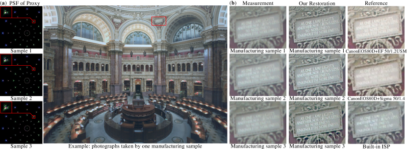
Figure 1: Manufacturing biases adaptation and comparisons. (a) centrosymmetric PSF calculated by the proxy camera of different machining samples (Best viewed with zoom). (b) magnified comparisons of the photographs taken in the same scene. We show the measured degradation of each Phone (converted to sRGB for visualization) and our restoration output from the same ISP pipeline. And the results of high-end DSLR cameras are shown for reference (captured under same aperture for comparisons).

This paper is devoted to a fundamental solution to ISP systems - bridging the gap between optics and postprocessing. We show an illustrative example in Fig. 1b, where the measurements of manufacturing samples are slightly different, yet the realized restorations are similar after processing. The classical ISP system is a step-by-step process where each module cascades with each other [16]. This separation mitigates the processing difficulty of each module but allows the slight errors accumulated in the subsequent operations [17]. To this end, recent works implement end-to-end methods for the mapping from Bayer pattern data to sRGB images [18]. However, the acquisition of densely-labeled data specified for each camera is time-consuming, and the enormous computational overhead is the critical limitation of deploying it into mobile terminals [19].

In this work, we mainly focus on connecting the optical design, the system manufacturing, and the ISP systems. A perturbation model is proposed for describing the influence of the deviated parameters on the geometric image evaluation, e.g., SFR. Distinct from the indicator calculation through exit pupil wavefront (used in optical design programs), we adopt the imaging simulation to obtain realistic photographs and apply SFR to measure MTF, which follows the process of image formation and index evaluation. It also provides an optimization framework to estimate the perturbed parameters from the measured indicators. In this way, a proxy camera, whose imaging results are close to reality, is constructed. It acts as a bridge for the co-design of the actual camera and the subsequent ISP.

Furthermore, we propose a brand new dynamic postprocessing architecture based on DOConv, expecting to handle the degradation of various system perturbations with one model. Engaging with the imaging simulation of the proxy camera, we encode the accumulated errors of cascaded modules and the degradation of system perturbations into the data pairs for the training of the dynamic model. This model realizes the correction of various machining samples’ optical degradations with less computational overhead. Our approach can be easily adapted into new camera devices at a penurious cost on indicator measurement, thus bypassing the time-consuming paired data collection.

We evaluate the proposed method on two imaging systems: customized digital single-lens reflex (DSLR) cameras and Huawei Honor 20 Pro (Phone), with known ideal optical parameters of both cameras. The assessments include the accuracy of constructing the proxy camera and the perturbation adaptability of the dynamic postprocessing model as well as the benefits to downstream vision applications (i.e., object detection, optical character recognition). Extensive experiments demonstrate that our method has the potential to link optical machining with postprocessing for realizing targeted restorations. The results are on par or sometimes even outperform the high-end DSLR lenses (the restoration results of Phones are shown in Fig. 1).

Our main contributions are summarized as follows:

• We construct a perturbed optical system model based on the image formation process, which illustrates the relationship between the perturbation of system parameters and the measured SFR. We demonstrate the advantage of the proposed perturbing model over the existing optical tolerancing procedure.

• We propose an optimization method to infer the system perturbation from the SFRs measured from actual manufacturing samples, hoping to construct proxy cameras whose imaging results are close to reality. These proxy cameras are to generate the data pairs that characterize the mapping of optical degradation, thereby fast adapting to the data acquisition of new devices in mass production.

• We propose a dilated Omni-dimensional dynamic convolution (DOConv) and implement it into post-processing to tackle spatially varying aberrations and stochastic machining deviations. It can be embedded into the existing ISP systems and correct the errors accumulated by modules cascade.

This paper proceeds as follows. In Section. 2, we review the related works. Section. 3 presents the optical perturbation model and the optimization to construct the proxy camera. The dynamic postprocessing pipeline is detailed in Section. 4. Quantitative and qualitative experimental analyses of our approach are provided in Section. 5. Section. 6 explores the potential applications of the proposed method. Conclusions and discussions are drawn in Section. 7.

2 Related Work

Optical degradation correction is a comprehensive mission in computational photography, where algorithms and optical systems cooperate. The additional machining bias poses a significant challenge to solving this problem. In this section, we present an overview of end-to-end optical system optimization and ISP systems.

2.1 End-to-End Optical System Optimization

Optical designers generally select the tolerance empirically or according to the performance requirements where the system bias is randomly sampled within tolerance to determine statistical degradation in mass production [20]. However, this process does not consider the actual machining procedure, which is meaningless for a particular manufacturing sample [1]. Besides the top-down tolerance analysis, considerable works infer the system parameters by polynomial (Zernike) fitting or convex optimization [7, 8, 21]. For polynomial fitting, the predicted range is generally broader than the actual for the multiple coefficients system [22]. Some works have taken advantage of the measured PSFs or images to fine-tune the entire system and perform targeted restoration [11]. However, the noise introduced in actual measurement can easily affect them since these methods are guided by the pixel-by-pixel mean squared errors (MSE) evaluation [14]. Recently, some works proposed to jointly optimize the optical parameters and the postprocessing systems in a differentiable manner, where the model of Fourier Optics [23], the image-to-image rendering [12], the proxy deep-learning model [13] are used to build the end-to-end pipeline. However, the end-to-end optimizations have some limitations when applied to complex systems with large FoV (in-depth discussions in the supplementary file).

We modify the ideal system to construct a proxy camera, whose system bias may not be precise compared to the actual device, but their imaging results are close. The proposed method guides the optimization by the geometric optical image evaluation, which is less susceptible to noise. We demonstrate that our physical-based framework can generate realistic imaging results for various machining samples and work under different noise levels.

2.2 Mobile ISP Systems

Considerable efforts have been invested in image postprocessing to correct optical degradation [24, 25, 26, 27, 28, 29]. Traditional deconvolution approaches utilize multiple image priors for iterative or mutual optimization to obtain the latent images [30, 31]. Unfortunately, they are inefficient in dealing with spatially varying degradation and thus have difficulty applying to real-time imaging [32]. The existing mobile ISP system divides the processing into multiple steps: white balance [33, 34, 35], denoising [36, 37], Bayer pattern interpolation [38, 39, 40], color correction [41], etc. Separating the task into independent modules facilitates the processing overhead, but the error of one module will be accumulated and magnified in subsequent steps, resulting in the wrong outputs [18].

Recent works propose to replace the cascaded ISP systems with deep learning models to address this issue [42, 19]. Such models are entirely data-driven and also have the potential for real-time imaging. [18] proposes to collect the data pairs by shooting the same scene with a mobile phone and a high-end DSLR. However, this data construction is time-consuming and has poor portability for new devices [43]. Recent works exploit to obtain data pairs by imaging simulation of an ideal system [28], but they do not consider the machining bias introduced during manufacturing. Therefore, there is a particular domain gap between the training data and the real-shot images, resulting in unsatisfied generalization for any processing samples in the actual scene [44].

Machining degradations introduced during camera production increase the difficulty of postprocessing algorithms. The deep learning methods mentioned above are fixed in the inference and cannot adaptively deal with the degradation of input features [45]. We noticed that many approaches apply attention or transformer to endow the network with dynamic processing ability [46, 47, 48, 49]. On a large scale of data, these models have a better performance than the static model, yet in the data with a relatively single distribution, they tend to overfit [50, 51].

In this work, multiple proxy cameras are engaged to synthesize realistic data for the training of the dynamic model. The proposed method successfully restores the optical degradation of complex distribution and realizes adaptive postprocessing of samples with different deviations.

3 Perturbed Optical System Model

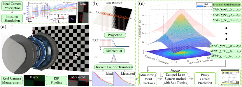
Figure 2: Overview of the perturbed optical system model. (a) We simulate the imaging results of the ideal edge by the camera’s parameters (top) and acquire the measured edge by photographing with real devices (bottom). (b) The procedure from edge profile to SFR goes through projection, differential, and DFT. In this way, we obtain the SFRA of ideal design and the measured edge (detailed in Sec. 3.1.2). (c) Set the measured SFRAs as targets to optimize the system parameters and predict the proxy camera by damped least-squares iteration (detailed in Sec. 3.2).

With the lens prescriptions and the actual manufacturing sample, our goal is to construct a proxy camera whose imaging results are relatively close to the manufactured device. Different from the ideal designing procedure, geometric optical image evaluation such as the SFR generally suffers from the deviations introduced in manufacturing and mounting assembly. Moreover, the discrete sampling and noise of the sensor are non-negligible in measurement. Therefore, in the following Section. 3.1, we first analyze the image formation procedure of the perturbed optical system, aiming for constructing the relationship between the perturbation of system parameters and the measured SFR. Then in the Section. 3.2, the method to build a proxy camera is presented in a detailed account.

3.1 Geometric Optical Image Evaluation

A general camera is primarily divided into the optical lens and the photosensor, where the former gathers the scene information and the latter records the intensity of the signal. While due to the inevitable manufacturing deviation, the scene rays collected by the camera will be deflected unexpectedly during propagation, resulting in degraded images and unfavorable indicators. To model the perturbations of the system as well as their influence on the SFR measurement, we consider the case where an incident ray is traced in a camera modeled with biased coefficients.

3.1.1 Perturbed System Coefficients

Ray-surface intersection The spatial coordinates $(x,y,z)$ of an incident ray are as follows:

$$x=x_{0}+ks,y=y_{0}+ls,z=z_{0}+ms,$$ (1)

here $s$ is the parameter of distance along the ray measured from the source point $(x_{0},y_{0},z_{0})$, and $D=(k,l,m)$ are the normalized direction vector. The general surface encountered in mobile camera may be represented by:

$$\mathit{F}(x,y,z)=z-\frac{\widetilde{c}\rho^{2}}{1+\sqrt{1-(1+\widetilde{k})\widetilde{c}^{2}\rho^{2}}}-\sum_{j=1}^{\mathcal{N}}\widetilde{A}_{2j}\rho^{2j},$$ (2)

where $z$ is the coordinate along the optical axis. $\rho=\sqrt{x^{2}+y^{2}}$ is the distance from a surface point to the optical axis. $\widetilde{c}$ is the perturbed vertex curvature and $\widetilde{k}$ is the perturbed conic constant. $\widetilde{A}_{2j}$ is the $2j^{th}$ perturbed power aspherical coefficient where $\mathcal{N}$ is the total order of aspheric. To determine the ray-surface intersection, we apply the Newton-Raphson iteration method to find a value $s$ such that the coordinates value $(x,y,z)$ from Eq. (1) satisfy the surface Eq. (2). In every iteration $i$, the distance parameter $s$ is updated by:

$$s_{i+1}=s_{i}-\mathit{F}(x_{i},y_{i},z_{i})/\mathit{F}^{\prime}(x_{i},y_{i},z_{i}),$$ (3)

where $(x_{i},y_{i},z_{i})=(x,y,z)|_{s_{i}}$ and:

$$\mathit{F}^{\prime}(X_{i},Y_{i},Z_{i})=(F_{x})_{i}k+(F_{y})_{i}l+(F_{z})_{i}m,$$ (4)

here $(F_{x})_{i}$ denotes $\partial\mathit{F}/\partial x$ evaluated at $(x_{i},y_{i},z_{i})$. Similar calculations are performed with respect to $(F_{y})_{i}$ and $(F_{z})_{i}$. The iteration process is terminated with the value $s_{i}$ when

$$|s_{i}-s_{i-1}|<\epsilon^{\prime},$$ (5)

where $\epsilon^{\prime}$ is a small preassigned value that can be adjusted according to the required accuracy. After the intersection is determined, we follow the Snell’s law to carry out the direction vector after refraction:

$$\widetilde{n^{\prime}}\cdot\mathbf{D}^{\prime}\times\mathbf{r}=\widetilde{n}\cdot\mathbf{D}\times\mathbf{r},$$ (6)

here $\widetilde{n}$ and $\widetilde{n}^{\prime}$ are the perturbed refractive indices of the medium where the ray is incident and refracted, which is modeled by the material perturbation of d-light (i.e., refractive index $\widetilde{n}_{d}$ and abbe number $\widetilde{v}_{d}$). For the detailed material perturbation model, please refer to the supplementary file. $\mathbf{D}^{\prime}=(k^{\prime},l^{\prime},m^{\prime})$ is the unit vectors denoting the direction of refracted ray. $\mathbf{r}=(K,L,M)$ is a normal vector of the surface at the intersection. Indicating by Eq. (6), the coplanarity of vector $\mathbf{D}$, $\mathbf{D}^{\prime}$, and $\mathbf{r}$ allows us to represent $\mathbf{D}^{\prime}$ by the linear combination of $\mathbf{D}$ and $\mathbf{r}$:

$$\mathbf{D}^{\prime}=\mu\mathbf{D}+\Gamma\mathbf{r},$$ (7)

where $\mu=n/n^{\prime}$ and $\Gamma$ is an undetermined multiplier. Squaring and adding the component of Eq. (7), we obtain a quadratic in $\Gamma$, whose analytical solution is easy to solve:

$$\begin{split}&\qquad\qquad\quad\Gamma^{2}+2a\Gamma+b=0,\\ a&=\mu(kK+lL+mM)/(K^{2}+L^{2}+M^{2}),\\ b&=(\mu^{2}-1)/(K^{2}+L^{2}+M^{2}),\end{split}$$ (8)

Surface-to-surface transfer Apart from the tracing procedure in a rotationally symmetric system, the tilts of optical elements are significant factors to be reckoned with when light propagates in a real camera. We model the incline of a surface in terms of Euler angles, where three successive rotations $\widetilde{t}_{zx}$, $\widetilde{t}_{yz}$, $\widetilde{t}_{xy}$ are to switch the ray data between the system of the optical axis and element:

$$\left(\begin{matrix}\overline{x}&\overline{k}\\ \overline{y}&\overline{l}\\ \overline{z}&\overline{m}\end{matrix}\right)=R\left(\begin{matrix}x-x_{\xi}&k\\ y-y_{\xi}&l\\ z-z_{\xi}&m\end{matrix}\right),$$ (9)

here $(x_{\xi},y_{\xi},z_{\xi})$ is the origin of the reference system. And the letters denoted by $\overline{(\cdot)}$ are the ray data of the transforming system. $R$ is expressed as follows:

$$\footnotesize\left(\begin{matrix}\cos{\widetilde{\gamma}}&-\sin{\widetilde{\gamma}}&0\\ \sin{\widetilde{\gamma}}&\cos{\widetilde{\gamma}}&0\\ 0&0&1\\ \end{matrix}\right)\left(\begin{matrix}1&0&0\\ 0&\cos{\widetilde{\beta}}&-\sin{\widetilde{\beta}}\\ 0&\sin{\widetilde{\beta}}&\cos{\widetilde{\beta}}\\ \end{matrix}\right)\left(\begin{matrix}\cos{\widetilde{\alpha}}&0&-\sin{\widetilde{\alpha}}\\ 0&1&0\\ \sin{\widetilde{\alpha}}&0&\cos{\widetilde{\alpha}}\\ \end{matrix}\right),$$ (10)

where $\widetilde{\alpha}=\widetilde{t}_{zx}$, $\widetilde{\beta}=\widetilde{t}_{yz}$, $\widetilde{\gamma}=\widetilde{t}_{xy}$ are the angles between the reference system and the transforming system.

After system transformation, the propagation from one surface to the next surface is first addressed by tracing the ray following the perturbed thickness vector $\widetilde{d}$ (represented by the norm $\widetilde{l}$ and the direction cosine $(\widetilde{d}_{x},\widetilde{d}_{y},\widetilde{d}_{z})$):

$$s=(\widetilde{l}\cdot\widetilde{d}_{z}-\overline{z})/m,x=\overline{x}+ks-\widetilde{l}\cdot\widetilde{d}_{x},y=\overline{y}+ls-\widetilde{l}\cdot\widetilde{d}_{y},$$ (11)

In this way, we model the perturbation of thickness and decenter in the meanwhile. For the detailed decenter illustration, please refer to the supplementary file. After the propagation between two surfaces, the ray data is transformed into the system of the latter surface by Eq. (9). And the aforementioned steps are repeated for succeeding surfaces in sequence until the sensor plane, where the ray data and the optical path length of each ray are recorded.

In summary, the perturbed optical system as well as its impact on incident ray are modeled through surface-by-surface ray tracing. We consider the potential perturbation of all optical elements to construct an authentic model based on physical procedure (the specific configurations are listed in the supplementary file). The recorded ray data is used to establish the link between perturbed coefficients and the SFR measurement, which will be illustrated in the following.

3.1.2 SFR Measurement via Imaging Simulation

In the optical design process, the MTF of the imaging system is obtained by Fourier transforming the continuous wavefront on the exit pupil plane. However, in the geometric optical image evaluation, the SFR (equivalent to the system’s MTF) is generally obtained by the Fourier transform of the line spread function (LSF) captured by the sensor. As demonstrated in the Appendix A of the supplementary file, the discrete sampling of the sensor and the noise will make differences in SFR. Therefore, we adopt the imaging simulation technique to synthesize a realistic edge image to ensure the procedure of calculating SFR between simulation and measurement is similar. In imaging simulation, the diffraction effect caused by the optical aperture is another content to be considered in addition to the aberrations calculated by tracing. So we inverse the tracing ray (calculated in Section. 3.1.1) from the sensor plane to the exit pupil and consider each ray as a source of the Huygens wavelet. Denoting the coordinates of ray on pupil plane is $(x^{\prime},y^{\prime},z^{\prime})$ and on the sensor plane is $(x^{\prime\prime},y^{\prime\prime},z^{\prime\prime})$, the complex amplitude on the sensor is superpositioned by the complex amplitude of spherical wavelet:

$$\mathbf{E}_{x^{\prime\prime}y^{\prime\prime}}(\mathbf{l}_{x^{\prime}y^{\prime}},\mathbf{r}_{x^{\prime\prime}y^{\prime\prime}},\mathbf{K})=\sum_{y^{\prime}}\sum_{x^{\prime}}a_{0}\frac{e^{ik\mathbf{l}_{x^{\prime}y^{\prime}}}}{\mathbf{l}_{x^{\prime}y^{\prime}}}\frac{e^{ik\mathbf{r}_{x^{\prime}y^{\prime}}}}{\mathbf{r}_{x^{\prime}y^{\prime}}}\mathbf{K},$$ (12)

where $l_{x^{\prime}y^{\prime}}$ is the optical path length from the source $(x_{0},y_{0},z_{0})$ to $(x^{\prime},y^{\prime},z^{\prime})$. $k=2\pi/\lambda$ and $\lambda$ is the wavelength of the ray. $r_{x^{\prime\prime}y^{\prime\prime}}=(x^{\prime\prime}-x^{\prime},y^{\prime\prime}-y^{\prime},z^{\prime\prime}-z^{\prime})$ indicates the direction of wavelet’s propagation. $\mathbf{K}$ is the obliquity factor of wavelet, which is defined as follows:

$$\mathbf{K}(\mathbf{D}_{x^{\prime}y^{\prime}},\mathbf{r}_{x^{\prime\prime}y^{\prime\prime}},\mathbf{n})=\frac{1}{2}[\cos{\langle\mathbf{n},\mathbf{r}_{x^{\prime\prime}y^{\prime\prime}}\rangle}-\cos{\langle\mathbf{n},\mathbf{D}_{x^{\prime}y^{\prime}}\rangle}],$$ (13)

where $\mathbf{n}$ is the normal unit vector of the exit pupil plane and $\cos{\langle\cdot,\cdot\rangle}$ is the operation of computing the cosine value of the two vectors. The relationships of $\mathbf{n}$, $\mathbf{D_{x^{\prime}y^{\prime}}}$, and $\mathbf{r_{x^{\prime\prime}y^{\prime\prime}}}$ are magnified in Fig. 2. The complex amplitude is multiplied with its conjugate to obtain the intensity on sensor plane:

$$I_{x^{\prime\prime}y^{\prime\prime}}=\mathbf{E}_{x^{\prime\prime}y^{\prime\prime}}\cdot\mathbf{E}^{*}_{x^{\prime\prime}y^{\prime\prime}},$$ (14)

In this way, we obtain the PSF $I_{fovi}(\lambda)$ at different wavelengths of this FoV. The imaging simulation of edge is:

$$J_{e}=\int\mathcal{C}_{e}(\lambda)\cdot I_{fovi}(\lambda)d\lambda*L_{e}+N_{e}.$$ (15)

here $\mathcal{C}_{e}(\lambda)$ is the sensor wavelength response. $J_{e}$, $L_{e}$, and $N_{e}$ are the observed edge, the latent ideal edge, and the sythetic noise image, respectively. We refer readers to [28] for details on imaging simulation implementation.

After simulating the degraded edge that resembles the actual observation, we measure the SFR as the procedure shown in Fig. 2b. First, we project all pixels along with the inclination to obtain the edge spread function (ESF). Second, a quarter of the pixel size $p_{i}$ is as the new sampling interval, and all pixel values that fall within the same sampling interval are averaged to represent the values of the resampling interval $i$. This operation is the key to alleviate the influence of noise. Third, we get LSF by the differentiation of ESF and calculate the discrete Fourier transformation of LSF. The normalized amplitude of the Fourier spectrum is the measured SFR. In this way, we construct a physical-based procedure to bridge the gap between the perturbed system parameters and the SFR measurement.

3.2 Proxy Camera Construction

In this section, we present an optimization framework to construct a proxy camera so that its imaging simulation is similar to the photograph of the target device. As illustrated in Section. 3.1, due to the highly nonlinear relationship between SFR and perturbed system parameters, it is impossible to predict the actual deviation of the camera analytically. So successive iterations are needed to approximate the solution. However, directly setting the SFR sequence as the target is unrealistic, where the computational overhead will increase exponentially when the sampling density grows. Therefore, SFR Area (SFRA), which is the area between the real measured SFR and the axis, is used as the target for optimization:

$$SFRA^{*}_{fovi}=Area(SFR),$$ (16)

We use the damped least-squares method to obtain the system solution of proxy camera [52]. Let the perturbed parameters illustrated in Sec. 3.1.1 denoted by $p_{1},p_{2},\cdots,p_{N}$, where $N$ is the number of parameters. The simulated SFRA calculation can be represented by:

$$SFRA_{fovi}=Area[F_{fovi}(p_{1},p_{2},\cdots,p_{N})],$$ (17)

here $F_{fovi}$ indicates the operation to calculate SFR by the method detailed in Sec. 3.1. The damped merit function $\phi(\vec{P})$ in matrix-vector form is constructed as follows:

$$\phi(\vec{P})=\vec{f}^{T}\vec{f}+\epsilon\Delta\vec{P}^{T}\Delta\vec{P},$$ (18)

where $\epsilon$ is the damped factor. $\Delta\vec{P}$ and $\vec{f}$ are as follows:

$$\begin{split}\vec{P}_{k+1}&=(p^{k+1}_{1},\cdots,p^{k+1}_{N})^{\mathrm{T}},\vec{P}_{k}=(p^{k}_{1},\cdots,p^{k}_{N})^{\mathrm{T}},\\ \Delta\vec{P}_{k}&=\vec{P}_{k+1}-\vec{P}_{k},\qquad\quad\;\vec{f}=(f_{1},f_{2},\cdots,f_{M})^{\mathrm{T}},\end{split}$$ (19)

$\vec{P}_{k+1}$ and $\vec{P}_{k}$ are the system parameters after $k$, $k+1$ iterations. $\Delta\vec{P}_{k}$ is the predicted linearity correction. $\vec{f}$ is the difference vector, where $f_{i}=SFRA^{*}_{fovi}-SFRA_{fovi}$ and $M$ is the number of sampled FoVs. According to the extreme value theory of multivariate function, the minimum of the merit function is achieved where its gradient is zero:

$$grad\;\phi(\vec{P})=A^{\mathrm{T}}\vec{f}+\epsilon\Delta\vec{P}=0,$$ (20)

here $A\in\mathbb{R}^{M\times N}$ is the partial derivative matrix ($A_{mn}=\partial f_{m}/\partial p_{n}$, where $m\in[1,M]$ and $n\in[1,N]$), which can be calculated by divided differences in implementation.

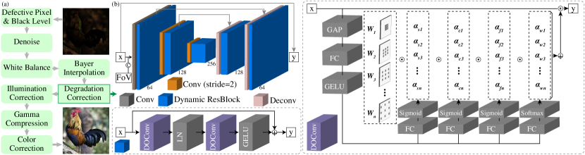
Figure 3: Overview of the dynamic postprocessing pipeline. (a) an optical degradation correction module is embedded into the ISP pipeline of mobile terminal. (b) we propose a dynamic postprocessing model based on dilated Omni-dimensional dynamic convolution, aiming at self-adaptively tackling the stochastic manufacturing deviation. All the layer configurations are marked with different colored blocks.

Unfortunately, the $\vec{f}$ is a non-linear function where the variable $\vec{P}$ cannot be solved directly. Hence, linear approximation is made by the Taylor series of $\vec{f}$ at $\vec{P}_{k}$:

$$\hat{f}=\vec{f}_{k}+A\Delta\vec{P}_{k},$$ (21)

where the $\vec{f}_{k}$ is the $\vec{f}$ of deviated parameters $\vec{P}_{k}$. We note that the approximation only guarantee linear accuracy in a small range of $\vec{P}_{k}$, so damping is set on $\Delta\vec{P}_{k}$ to control the step. Replacing the $\vec{f}$ in Eq. (20) by Eq. (21), we derive the $\Delta\vec{P}_{k}$ after $k$ iteration:

$$\Delta\vec{P}_{k}=-(A^{\mathrm{T}}_{k}A_{k}+\epsilon I)^{-1}A^{\mathrm{T}}_{k}\vec{f}_{k}.$$ (22)

here $A_{k}$ is the $A$ of $\vec{P}_{k}$, $I$ is the identity matrix. And the predicted system parameters are $\vec{P}_{k+1}=\vec{P}_{k}+\Delta\vec{P}_{k}$ after $k+1$ iteration.

Algorithm 1 Proxy Camera Construction

0:  System parameters $\vec{P}_{0}$ , Measured $SFRA^{*}_{fovi}$

1:  $k\leftarrow 0$, and $\vec{f}_{k},A_{k}\leftarrow Merit(\vec{P}_{k},SFRA^{*}_{fovi})$

2:  while $||A^{\mathrm{T}}_{k}\vec{f}_{k}+\epsilon\Delta\vec{P}_{k}||\gg 0$ do

3:     $\Delta\vec{P}_{k}\leftarrow-(A^{\mathrm{T}}_{k}A_{k}+\epsilon I)^{-1}A^{\mathrm{T}}_{k}\vec{f}_{k}$

4:     $\vec{P}_{k+1}\leftarrow\vec{P}_{k}+\Delta\vec{P}_{k}$

5:     $k\leftarrow k+1$, and $\vec{f}_{k},A_{k}\leftarrow Merit(\vec{P}_{k},SFRA^{*}_{fovi})$

6:  end while

7:  return  $\vec{P}_{k}$

8:  Function: $Merit(\vec{P}_{k},SFRA^{*}_{fovi})$

9:  for i=1:M do

10:     Edge imaging simulation with Eq. (1) - Eq. (15)

11:     Measure SFRA from synthetic edge as Fig. 2b

12:     $\vec{f}_{i}\leftarrow SFRA^{*}_{fovi}-SFRA_{fovi}$

13:     for j=1:N do

14:        $A_{ij}=(\vec{f}(\cdots,p^{k}_{j}+\Delta p_{j},\cdots)-\vec{f}_{k})/\Delta p_{j}$

15:     end for

16:  end for

17:  return  $\vec{f}_{k}$, $A_{k}$

We also note that each system parameter contributes differently to the merit functions. Therefore, we dynamically adjust the damping factor $\epsilon$ of each parameter according to the non-linearity of the solution $\Delta\vec{P}$, which is detailed in the supplementary file. In this way, the optimization is performed from Fig. 2a to Fig. 2c until the gradient of solution (Eq. (20)) is close to zero.

Altogether, we illustrate the perturbed optical system model and the method to construct a proxy camera based on the measurement of SFR. There are three significant advantages between the proposed method and other end-to-end optimizing approaches in Section 2.1. First, our optimization framework is insensitive to noise because of the resampling in SFR measurement. Second, our imaging simulation considers the diffraction effect caused by the optical aperture and therefore is more accurate than bare ray tracing. Third, we consider the potential perturbation of all elements which is more authentic in following the physical procedure (in-depth comparisons are presented in supplementary file). Hence, we engage the proxy camera with the physical formation pipeline of raw images to perform authentic imaging simulation, generating the data pairs for deep-learning-based reconstruction.

4 Dynamic-processing ISP

To eliminate the camera-wise manufacturing deviations and spatially varying optical aberrations, the ability of self-adaptive correction is necessary for the postprocessing pipeline. Moreover, the computational overhead of the mobile terminal puts a significant limit on the complexity of the model. To this end, we propose a lightweight framework based on dynamic convolution to meet the needs of adaptive processing and the constraints in application. In the following Section. 4.1, we first illustrate the data preparation for the training of the framework. Then in the Section. 4.2, the proposed postprocessing pipeline is detailed.

4.1 Data Preparation

Based on the virtual camera constructed in Sec. 3, we construct the training data pairs by the imaging simulation in Sec. 3.1.2. Since the exposure parameters of real photography are discrete, the dynamic range of the captured raw image is not ideal. Therefore, we add luminosity compression/decompression in simulation which is different from the transformation in [28]. After obtaining the raw-like image, the formation of the sensor observation with optical degradation can be formulated as:

$$J_{e}(x,y)=\int\mathcal{C}_{e}(\lambda)\cdot I_{fovi}(x,y,\lambda)d\lambda*L_{e}(x,y)+N_{e},$$ (23)

here $(x,y)$ is the pixel coordinates on the sensor plane. And the rest denotions are the same as Eq. (15). We note that the performance of optical degradation on the raw image is linear and channel-irrelevant. So different from [28], we abandon the CCM and the gamma compression in the synthetic pipeline after adding the degradation into the image. Because these operations will introduce non-linearity and cross-channel information, thus increasing the difficulty of restoration. Because of the limited number of manufacturing samples, the proxy cameras could not cover the distribution of manufacturing deviation. So we regard the max bias of each system parameter as the tolerance and random sample them to generate more virtual optical systems for data generation. This augmentation allows the model to learn the potential degradation and prevents overfitting. In this way, we obtain the RAW-to-sRGB data pairs, which characterize the mapping of optical degradation and encode the accumulated errors of cascaded modules. The data pairs not only follow the physical procedure of image formation but also are friendly to the training of the deep-learning method.

4.2 Dynamic Postprocessing based on DOConv

The stochastic manufacturing deviations and spatially varying optical aberrations cause different PSFs on the sensor plane. However, the traditional convolution operation strictly receives the feature by fixed weight and locations around its center, which is hard to adapt to the stochastic degradation and introduce relevant information into the output. To this end, we propose a dynamic convolution model for eliminating the optical degradation and embed it in the traditional ISP pipeline to realize extreme quality computational imaging. Inspired by the idea in [47], we design the dilated Omini-dimensional dynamic convolution (DOConv) and implement it into a variant of UNet architecture. As shown in Fig. 3, each DOConv has four weights, and their dilations vary from 1 to 4 in implementation, aiming at performing targeted feature acquisition. We reduce the stages of the architecture to mitigate the computational overhead. And the ResBlocks, whose internal components are the same as the Block in [49], are applied in each scale to enhance the expression ability. The model takes degraded raw-like data as input and outputs restored images in the same domain. Subsequently, the restorations are processed by the subsequent modules and supervised by the sRGB ground-truth. Since the generated data pairs are pixel-to-pixel aligned and cover all potential degrading distributions, it is sufficient to train the model only relying on fidelity losses:

$$L(\theta)=\frac{1}{N}\sum^{N}_{n=1}||Process(Model(J^{n}_{e}))-L^{n}||^{2}_{2}.$$ (24)

where $\theta$ denotes the learned parameters in the model. $J^{n}_{e}$ are the degraded raw image and $L^{n}$ are the corresponding sRGB ground-truths. $Process(\cdot)$ denotes the subsequent operations after optical degradation correction.

5 Experiments

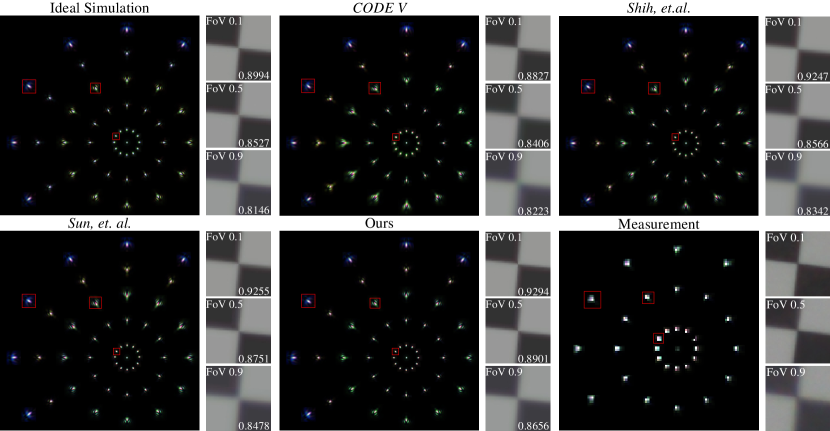
Figure 4: Qualitative evaluation on PSF and imaging simulation. We visualize the centrosymmetric PSFs ($10\times$resampling for detailed comparisons) of the proxy cameras constructed from one machining sample of the Phone (the measured PSFs are shown in the sensor resolution). For the proxy camera, the resolutions of PSFs are 50, 50, 80, 80, and 120 of FoV 0.1, 0.3, 0.5, 0.7, and 0.9, respectively. And in measurement, the resolutions of PSFs are 5, 8, and 12 for FoV 0.1, 0.5, and 0.9. We present the imaging simulation results and their SSIM compared with actual measurements.

We first roughly illustrate the experimental setting in Section. 5.1. In Section 5.2, comprehensive experiments are conducted to demonstrate the theoretical advantage of the proposed proxy camera construction. In Section 5.3, we evaluate the strength of the proposed dynamic model when tackling optical degradation. Finally, an in-depth ablation study is presented in Section 5.4.

5.1 Experimental setting

To substantiate the authenticity of the proposed proxy camera construction, we evaluate two devices, one is a customized DSLR camera, and another one is Huawei Honor 20 Pro (Phone). The optical prescriptions of both cameras are known, and their system parameters are listed in the supplementary file. In edge measurement (Fig. 2a), we rotate the targets at $9\sim 12^{\circ}$ angles and take photos of them. And the ideal edge is colored according to the dynamic range of the measured edge. For SFRA measurement (Fig. 2b), the sampled FoVs are the regions that evenly divide the image into $15\times 20$. In training data construction, we first calculate the PSFs of the proxy camera following Eq. (14). Then the PSFs of different FoVs are used to degrade the latent image as Eq. (15). We acquire the latent image by adopting DIV2K [53] and rescaling these data to the resolution of the camera (DSLR is $4000\times 6000$ and Phone is $3000\times 4000$). In terms of the hyperparameters of training, the channel of each layer is marked at the block bottom, the model is trained with ADAM optimizer [54] ($\beta_{1}=0.9$, $\beta_{2}=0.999$, $\epsilon=10^{-8}$), and the learning rate starts at $10^{-4}$ then halved every 10 epochs. The setting of dynamic convolution is the same as [47]. For more implementation details about the proposed framework, please refer to the supplementary file.

5.2 Authenticity of Proxy Camera Construction

5.2.1 Competing Methods

To demonstrate the advantages of the proposed approach, we compare our method with these representative methods

1. The built-in tolerance analysis of optical design software, i.e., MTF tolerance of $CODEV^{\circledR}$ [8].

2. Modify the optical parameters by the calibrated PSFs, i.e., shih, et. al. [11].

3. Optimize the system by image-to-image rendering through differentiable ray tracing, i.e., sun, et. al. [12].

Since the tolerancing in commercial software only derives the deviation range, we choose the prediction’s median as the bias for each parameter. In the second method, we use pixel-level MSE between the simulated and measured PSFs to guide the optimization. Noting that there are alternative end-to-end system optimization besides the third method, we present an in-depth comparison in the supplementary file to illustrate the reason we pick this method.

5.2.2 Quantitative and Qualitative Assessment

TABLE I: Quantitative proximity between real devices and proxy camera. Note that the value is the average of all machining samples. The best and the second-best indicators of each FoV are marked in red and blue.

CAMERA	Method	MSE ($\times 10^{-3}$) $\downarrow$	SSIM $\uparrow$
		FoV 0.1/0.5/0.9	FoV 0.1/0.5/0.9
DSLR	Ideal	0.576/0.804/1.023	0.913/0.906/0.872
	$CODEV^{\circledR}$	0.521/0.764/1.242	0.899/0.874/0.833
	shih, et. al.	0.374/0.714/0.958	0.951/0.932/0.917
	sun, et. al.	0.407/0.708/0.924	0.942/0.929/0.920
	Ours	0.382/0.698/0.877	0.946/0.938/0.922
Phone	Ideal	0.814/1.621/1.768	0.896/0.854/0.806
	$CODEV^{\circledR}$	0.852/1.746/1.496	0.878/0.842/0.822
	shih, et. al.	0.643/1.386/1.325	0.913/0.858/0.832
	sun, et. al.	0.628/1.303/1.157	0.915/0.872/0.847
	Ours	0.547/1.251/0.952	0.927/0.887/0.859

To illustrate the authenticity of the proposed optimization, we evaluate the proximity of the proxy camera (by the MSE between the simulated and the measured discrete SFR) and the similarity of imaging (by SSIM [55] between images). The indexes of all machining samples are averaged for comparison, and the ideal simulations are provided for reference. As shown in Tab. I, the competing methods generally perform better on the DSLR than on the Phone. These phenomena attribute to 1) the aberration of DSLR increases uniformly with the growth of FoV, yet the degradation of Phone changes significantly, which increases the difficulty in prediction; 2) the relative illumination of PHONE decreases a lot in marginal FoV, resulting in a declining Signal-to-Noise ratio (SNR). So for the optimizing method that relies on pixel-level indicators (shih, et. al. and sun, et. al.), it is challenging to extract undisturbed information from actual noisy measurements. In terms of evaluation metrics, our method constructs the proxy systems that are the closest to the machined devices, especially in difficult situations such as low SNR and highly non-uniformed degradation.

The visualization of PSF calculation and the imaging simulation of all competing methods are shown in Fig. 4. Limited by the space, we only present the resampling PSFs and imaging simulation of some FoVs. Moreover, the ideal simulation and the actual measurement are provided for reference, and the SSIM of each simulated patch is listed for additional quantitive evaluation. As shown by the PSFs of the same FoV, all methods roughly predict the eccentricity of the device. We note that the degradation caused by the predicted deviations of $CODEV^{\circledR}$ is more severe than the actual measurement, which is because it calculates the influence of each system variable separately without considering the combined impact of the entire lens. shih, et. al. and sun, et. al. have poor accuracy when the FoV increases due to the pixel-level metric disturbance introduced by the magnified noise level in edge FoV. sun, et. al. obtains more accurate simulation results than $CODEV^{\circledR}$ and shih, et. al.. But since the ray tracing does not consider the diffraction of optical aperture, its predicted perturbation is often larger than our estimation, resulting in more significant degradation. By contrast, our method produces accurate results not only on visual similarity but also from quantitative assessment. More discussions are presented in the supplementary file.

5.2.3 Noise Injection Influence

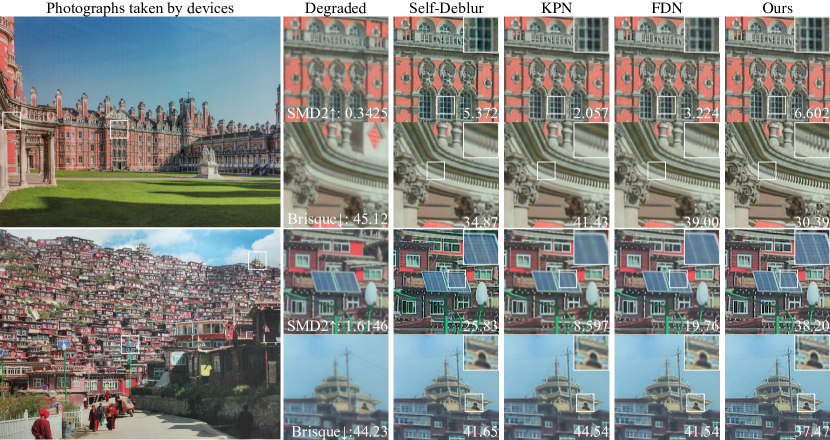
Figure 5: Non-uniform deblurring on real photographs of Phone. We mark the corresponding regions with white boxes and present the indicators.

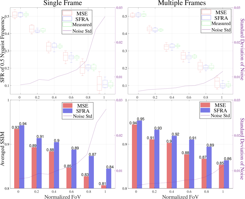
Figure 6: Performance under different noise level. The left/right part shows the accuracy of proxy camera construction under single/multiple frames. The upper/lower part presents the MTF/SSIM evaluation. The noise level is plotted in the purple line.

The crucial merit of our approach compared to optimizing with pixel-level evaluation is that the measuring procedure of SFRA is insensitive to the noise of actual photographs. We analyze the statistical results when using pixel-level MSE and SFRA as optimization objectives under different noise situations. The left part and the right part of Fig. 6 show the different FoVs’ accuracy on the single-frame image and the multi-frames image (superposed for denoising), respectively. The evaluation in the upper part of Fig. 6 is the SFR at 0.5 Nyquist frequency, and the lower part is the SSIM between the simulation and the actual photograph. We note that the variance of noise (indicated by the purple line) grows as the FoV increases because of the decreasing illumination by lens shading. Thus the optimization targeted with MSE is prone to severe fluctuations due to this metric being easily affected by accidental errors when the noise level increases. On the contrary, the proposed method maintains similar-to-real SFR fluctuation and higher SSIM evaluation under different noise levels. This mainly benefits from the resampling ESF operation (projecting all pixels along with the inclination and averaging the values), which makes the SFRA insensitive to the noise and provides stable guidance for our optimization.

5.3 Evaluation on Dynamic Postprocessing

5.3.1 Competing Methods

The performance of optical degradation on the image can be integrated as the influences of spatially varying blur on different FoVs. Therefore, correcting the optical degradation can be summarized as a deblurring task. we collect the state-of-the-art deblurring algorithms for comparisons

1. Global deblurring method, i.e., scale recurrent network (SRN) [56] and Self-Deblur (SD) [57].

2. Kernel-based deblurring method, i.e., kernel prediction network (KPN) [58].

3. Dynamical-adjusted deblurring method, i.e., FoV deformable network (FDN) [28].

For these algorithms, we apply the same RAW-to-sRGB data for evaluation. The details of training and inference procedure are presented in the supplementary file.

5.3.2 Results on non-uniform deblurring

TABLE II: Quantitative results on sythetic data and real photographs. C denotes the evaluated platform. T is the training datasets, where single sample means the data pairs are synthetic by one proxy camera and multiple samples means altogether evaluation on multiple virtual cameras. The best and the second-best indicators of each evaluation are marked in red and blue. We indicate the better metrics with up/down arrows.

C	T	Method	Evaluation on Synthetic Data				Real Photographs		T	Evaluation on Synthetic Data				Real Photographs
			PSNR $\uparrow$	SSIM $\uparrow$	VIF $\uparrow$	LPIPS $\downarrow$	BRISQUE $\downarrow$	NIQE $\downarrow$		PSNR $\uparrow$	SSIM $\uparrow$	VIF $\uparrow$	LPIPS $\downarrow$	BRISQUE $\downarrow$	NIQE $\downarrow$
DSLR	Single Sample	SNR	42.19	0.984	0.988	1.383	39.80	3.846	Multiple Samples	40.84	0.973	0.967	1.839	42.82	4.153
		SD	42.58	0.988	0.989	1.178	38.51	3.258		40.97	0.976	0.970	1.678	40.88	3.868
		KPN	41.86	0.987	0.982	1.186	43.28	3.729		40.57	0.977	0.966	1.523	45.86	4.257
		FDN	43.12	0.992	0.996	0.757	40.57	2.924		41.94	0.985	0.987	1.212	42.89	3.505
		Ours	43.03	0.991	0.993	0.924	36.56	3.213		42.12	0.986	0.990	1.241	38.88	3.431
Phone		SNR	33.26	0.957	0.943	2.264	43.27	4.674		30.17	0.928	0.907	3.248	47.91	5.347
		SD	34.03	0.959	0.946	1.966	41.77	4.185		30.33	0.930	0.913	3.017	45.86	4.928
		KPN	32.96	0.963	0.939	1.525	44.66	4.527		29.96	0.938	0.901	2.476	48.57	5.267
		FDN	34.56	0.974	0.968	0.984	42.71	3.644		31.86	0.942	0.922	1.897	46.59	4.056
		Ours	34.28	0.976	0.964	1.084	39.88	3.713		32.28	0.950	0.938	1.584	43.68	4.131

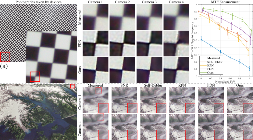
Figure 7: Adaptation for manufacturing deviation. (a) we show the magnified patch to illustrate the image quality mutation of Phone. The actual checkers’ restoration of different machining samples are present for comparison. And we evaluate the average SFR (MTF) enhancements on the machining samples of test set. (b) the natural photograph restoration when applied on different machining samples of Phone.

To evaluate the ability of various methods to handle non-uniform optical degradation, we train all the compared methods on the data generated by one proxy camera. Fig. 5 shows the various methods’ restoration in different FoVs of real photographs and presents the BRISQUE [59] and SMD2 [60] for evaluation. The quantitative evaluation of non-uniform deblurring is provided in Tab. II, where the single sample of T is the assessment on one proxy camera. We apply the reference image quality assessments (IQA), e.g., PSNR, SSIM [55], VIF [61], and LPIPS [62] to evaluate synthetic data. And the non-reference IQAs, e.g., BRISQUE [59], NIQE [63] are assessing real photograph because obtaining non-degraded reference of real photo is impossible.

For the globally consistent deblurring method, it can be seen that the deterioration is suppressed. However, since the optical aberration is spatially variant, the restoration is a compromise of each FoV: in the center FoV with less blurring, ringing, and color artifacts shows up on the border of objects, while in the case of severe degradation at the edge of the image, the optical aberration is not fully corrected. When it comes to the kernel-based method, KPN can cope with the non-uniform degradation, benefiting from the ability to predict the spatially varying kernel according to the input features. However, since the blurring is associated with the FoV and these models are not aided by FoV information, such methods are confused by the input features and generate incorrect restoration results. For the approach that adjusts processing according to the FoV, FDN can better tackle the FoV-related optical aberration and obtain competitive results when correcting a specific camera (shown in Tab. II). Our model realizes competitive results in both visual quality and metrics. We note that we outperform the FDN in BRISQUE, which may be because this metric pays more attention to the details of the image. The dynamic convolution model generally suffers from overfitting when the data distribution is relatively singular. But our method fits the degradation of the actual measurement well when only depending on the synthetic data of one proxy camera, which may be due to the dilation manner so that different weights have different specializations for adaptive processing.

5.3.3 Adaptation for Manufacturing Deviation

In mass production, there is no time to specifically train each post-processing model for a particular camera. To this end, the restoration must be able to cope with the stochastic deviation introduced in manufacturing and assembly. To evaluate the ability to tackle this task, we simultaneously train the competing methods with the data generated by various virtual cameras. Fig. 7a and Fig. 7b show the results of different models dealing with the camera-wised degradation on the same scene. The measurement deteriorates more unpredictably due to random manufacturing deviation when the FoV increases, which enlarges the difficulty of restoration. Comparing the experimental results, we note that the static model (weights are fixed after completing training) cannot fit well in the diverse deviation of real manufacturing. In consequence, the static model fails to tackle the different machining degradations between real cameras, especially when FoV increases. Benefiting from the dynamic convolution, our model adaptively restores the degraded features and achieves better restoration results on each camera. The SFR enhancement (shown in the right part of Fig. 7a) demonstrates that the proposed method realizes better and more stable restoration. Other methods suffer from significant fluctuation when FoV increases. Additional quantitative evaluation of deviation adaptation presents in Tab. II. Other competing methods receive unfavorable results when the data distribution becomes complicated, while the proposed method maintains a high level.

5.4 Ablation Study

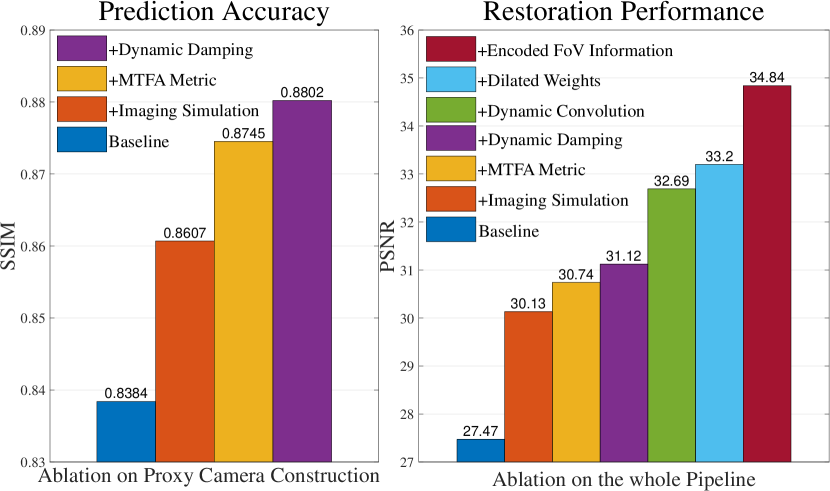
Figure 8: Ablation study on the proxy camera construction (accuracy evaluation on the SSIM between the simulated images and the natural photographs). And Ablation study on the whole pipeline (restoration assesment on the test synthetic data sets).

We first evaluate the prediction accuracy when ablating the crucial modules of virtual camera prediction. Then comprehensive ablation studies are conducted on our proposed method. Specifically, for the proxy camera construction: 1) we ablate the imaging simulation and calculate MTF by the continuous wavefront at the pupil plane. 2) we replace the MTFA with the MTF at 0.5 Nyquist frequency. 3) we substitute the dynamic damping strategy with a fixed damping factor. For the dynamic restoration: 1) the dynamic convolution layers are replaced by the ordinary convolution. 2) the dilation of each weight is the same; 3) encoded FoV information is ablated and only inputting image feature.

As shown in Fig. 8, the accuracy of prediction is significantly affected after ablating the imaging simulation module, which is mainly due to the inherent difference between the MTF calculation. One way is to compute by the continuous wavefront at the pupil plane, and another way is to obtain the SFR of the edge image (as demonstrated in the supplementary file). Moreover, using SFRA for optimization alleviates the influence of the measured SFR’s singular value in some spatial frequencies. And the dynamic damping ensures that the solution of perturbed parameters is linear within the damping range. Both of these modules facilitate the proposed framework more stable and efficient. For the evaluation of image restoration, the improvements in prediction accuracy are positively relevant. In the ablation of the reconstruction model, dynamic convolution performs a better fitting than traditional convolution when the distribution of data is more diverse. Meanwhile, the different dilations of weights also facilitate the correction of spatially-variant degradation. Finally, the encoded FoV information has a positive gain on restoration since the degradation is strongly associated with the pixel position on the sensor.

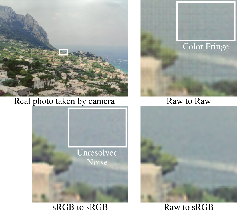
Figure 9: Ablation on the dynamic processing ISP. We evaluate the performance when placing the optical degradation correction model at different positions of ISP pipeline.

Figure 10: Comparisons with built-in ISP. Note that the built-in ISP smooths out the cords, yet our method restores it (marked with the red arrow).

In the proposed dynamic-processing ISP, we deploy the aberration recovery module between the Bayer interpolation and luminance correction. Its output is manipulated by the subsequent modules and compared with sRGB ground-truth in training. To prove the rationality of this deployment, we conducted the following ablation experiments: 1) Construct raw-to-raw data without considering subsequent operations for training; 2) Deploy the module at the end of the pipeline to construct sRGB-to-sRGB pairs for training. As shown in Fig. 9, the output of the model appears with colored stripes in raw domain reconstruction, which is because the network prediction does not take into account the subsequent operations, resulting in slight errors in the RAW domain are amplified in the subsequent processing. Restoration in sRGB also faces challenges, where the color noise is difficult to eliminate. This situation is because the color correction overlaps the information of each channel, which increases the difficulty of restoration. On the contrary, our method processes the input data in the RAW domain and supervises the output in sRGB, aiming at correcting the prediction error accumulated by the cascade pipeline.

6 Analysis

6.1 Comparisons with Built-in ISP

To demonstrate the significance of deploying the optical degradation correction, we compare our results with the built-in ISP. As shown in Fig. 10, the same JPEG compression algorithm is applied for the sake of a fair comparison. Due to the additional sharpening, the built-in ISP realizes similar results to ours in the center (Fig. 10-1). Yet this globally consistent operation fails to infer realistic features under severe degradation. Therefore, the advantage of our model is evident when it comes to the edge of photographs. The proposed pipeline adaptively restore the high-frequency details of leaves (Fig. 10-2) and cords (marked with the red arrow in Fig. 10-3) at the edge of FoV, which are smoothed out by the built-in ISP. Therefore, our dynamic model is well compatible with the existing ISP system and has the potential to correct the prediction error accumulated by the cascade pipeline. Moreover, our method endows post-processing with the ability to perform adaptive restoration according to the spatial information and the image feature.

6.2 Comparisons with deeplearning-based ISP

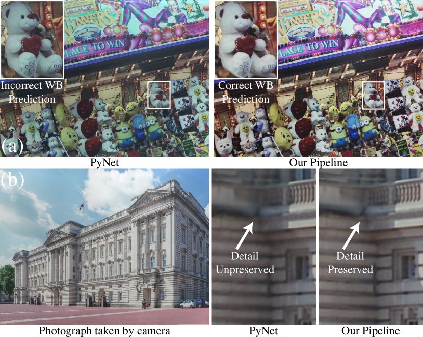
Figure 11: Comparisons with the deep-learning ISP. (a) the failure case of the deep-learning ISP in white balance prediction. (b) evaluation on the ability of detail preservation.

We note that many advanced postprocessing methods attempt to replace the entire ISP system with a deep learning model, called deep ISP. These methods rely on one complex architecture to perform super-resolution (equivalent to demosaic), brightness and color adjustment (equivalent to white balance and color correction), denoising, reconstruction, etc. on the captured Bayer image, output the pixel-by-pixel prediction. Due to the need to solve the altogether problems, such deep learning models are engaged with enormous parameters and are rough to implement into mobile terminals. Based on the proposed image formation simulation, we can also synthesize the data pairs from the degraded Bayer raw image to the ideal sRGB ground truth. Therefore, we train the advanced deep ISP model with the synthetic Bayer-to-sRGB data and evaluate the model on real-captured images. The comparisons of the deep ISP model and the proposed method are shown in Fig. 11. One can see in Fig. 11a, the PyNet cannot always predict the correct white balance gain when the scene is complicated, resulting in a bluish color of the white bear (magnified in the upper-left corner). Therefore, it is difficult for deep learning models to predict per-channel gain only from input features, let alone some metameric scenes. In view of this, we use the auxiliary white balance from the traditional ISP system to obtain the correct imaging result. We compare the ability of detail resilience in Fig. 11b when the deep ISP model predicts accurate gain and color correction. As shown, the deep ISP cannot reconstruct detailed textures. This situation is mainly due to the deep ISP model integrating multiple objectives into one model and using the same loss function to guide the restoration. The brightness and color gap between input and ground truth has a crucial influence on the fidelity loss, which will lead the model to eliminate this mismatch in the first place while ignoring the details of the image. In contrast, we separate each task and implement a dynamic model which corrects the postprocessing errors accumulated by the cascaded pipeline. Therefore, our method can accurately restore the color and brightness as well as the detailed information of the scene.

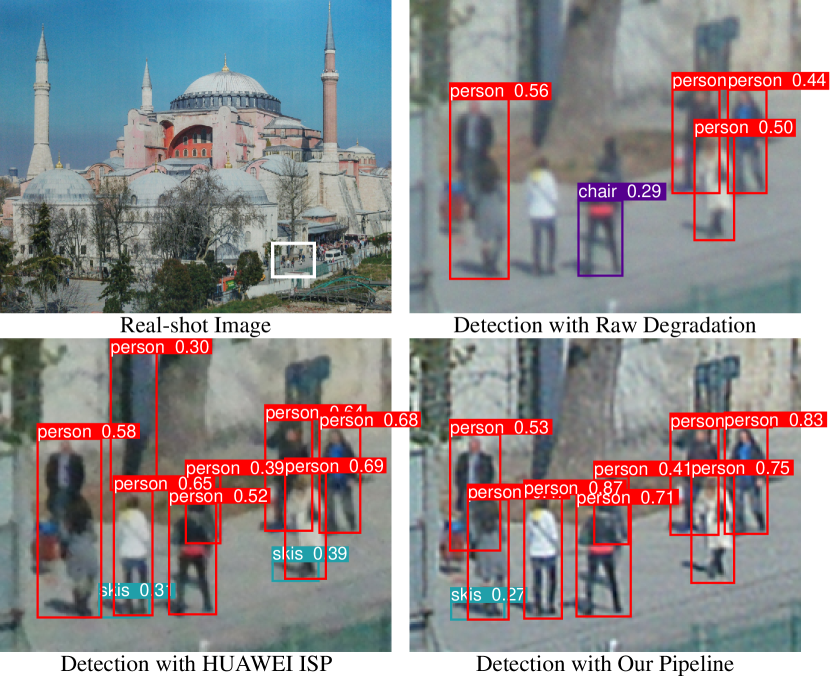
Figure 12: Object detection with different post-processing. The proposed method frees the SOTA detecting algorithms from fine-tuning for a specific camera in the implementation.

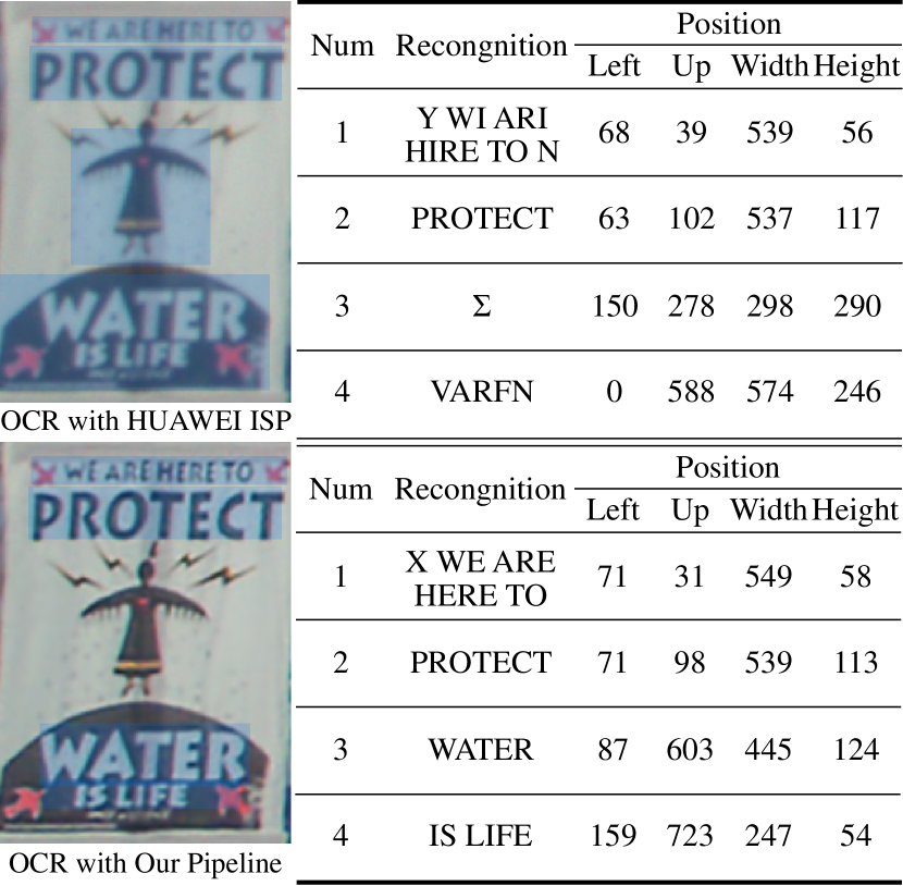
Figure 13: OCR with different post-processing. We help the advanced OCR framework for more accurate recognition and character position.

6.3 Application to Downstream Vision Tasks

The advantages of the proposed method, when applied to photographic postprocessing, have been illustrated before. We show that our pipeline could also be helpful for downstream computer vision applications, e.g., object detection, and optical character recognition (OCR). For the evaluation of these tasks, we follow the same pipeline as Fig. 3 to process the captured photographs and conduct off-the-shelf vision algorithms on the processed sRGB images. For comparison, we also show the results on the built-in ISP.

State-of-the-art methods are applied to the daily photos for evaluation, including YOLOv5 [64] for object detection and PaddleOCR [65] for OCR. In Fig. 12 and Fig. 13, we show the comparisons of visual and numerical results. As shown in Fig. 12, the detection with our pipeline accurately locates all people and gives higher confidence. But the detection with built-in ISP predicts the wrong location to some extent. When applied to OCR, PaddleOCR precisely determine the text regions and recognize text on our result, yet various errors occur in the built-in ISP. In conclusion, our algorithm can directly improve the performance of downstream vision applications, eliminating the need to fine-tune the algorithm for a specific camera.

7 Conclusion

We presented a perturbed camera model based on the image formation process. And an optimization framework was present to construct a virtual proxy camera from actually measured indicators, whose imaging results are close to the actual manufactured samples. With the proxy cameras from multiple machining samples, we synthesized the data pairs with complex degenerate distributions, aiming at encoding the optical aberrations and the random bias introduced during processing. Drawing from the dynamic convolution, we applied a dynamic model to self-adaptively cope with manufactured cameras, where multiple samples of two typical devices are evaluated to illustrate the benefits of the proposed pipeline. By training only with synthetic data, we demonstrated that our method successfully handles the system of complex machining deviations, achieving perfect restoration that outperforms the high-end DSLR camera.

Our work bridges the gap between optical design, system manufacturing, and postprocessing pipeline. It is convenient to deploy the proposed model in the mass production of arbitrary imaging devices. This work has been applied to some mobile terminals to realize significantly improved imaging. Nevertheless, some challenges remain unsolved to deploy our technique in production. First, for the specific system parameters and manufacturing methods (grinding for DSLR lenses and injection molding for cellphones), the introduced biases are complicated, rendering manual adjustment of damping factors in optimization. Not only that, many existing mobile terminals do not equip with the optimization for operations other than convolution, e.g., attention, which leads to low efficiency in mobile cameras. In conclusion, it is imperative to deploy an optical degradation correction module to the ISP system. As a bridge connecting the hardware system and the algorithm, it is of great help to improve the imaging quality and facilitate the downstream computer vision applications.

References

- [1] T. Lin and C. Cheng, “A novel opto-mechanical tolerance analysis method for precision lens systems,” Precision Engineering, vol. 35, no. 3, pp. 447–454, Jul. 2011. [Online]. Available: https://linkinghub.elsevier.com/retrieve/pii/S0141635911000304
- [2] C.-C. Hsueh, P. D. Lin, and J. Sasian, “Worst-case-based methodology for tolerance analysis and tolerance allocation of optical systems,” Appl. Opt., vol. 49, no. 31, pp. 6179–6188, Nov 2010. [Online]. Available: http://www.osapublishing.org/ao/abstract.cfm?URI=ao-49-31-6179
- [3] X. Hu and H. Hua, “Design and tolerance of a free-form optical system for an optical see-through multi-focal-plane display,” Appl. Opt., vol. 54, no. 33, pp. 9990–9999, Nov 2015. [Online]. Available: http://www.osapublishing.org/ao/abstract.cfm?URI=ao-54-33-9990
- [4] Q. Wang, D. Cheng, Y. Wang, H. Hua, and G. Jin, “Design, tolerance, and fabrication of an optical see-through head-mounted display with free-form surface elements,” Appl. Opt., vol. 52, no. 7, pp. C88–C99, Mar 2013. [Online]. Available: http://www.osapublishing.org/ao/abstract.cfm?URI=ao-52-7-C88
- [5] S. Jung, D.-H. Choi, B.-L. Choi, and J. H. Kim, “Tolerance optimization of a mobile phone camera lens system,” Appl. Opt., vol. 50, no. 23, pp. 4688–4700, Aug 2011. [Online]. Available: http://www.osapublishing.org/ao/abstract.cfm?URI=ao-50-23-4688
- [6] D. Malacara, Ed., Optical shop testing, 3rd ed., ser. Wiley series in pure and applied optics. Hoboken, N.J: Wiley-Interscience, 2007, oCLC: ocm74916130.
- [7] M. Rimmer, “Analysis of Perturbed Lens Systems,” Applied Optics, vol. 9, no. 3, p. 533, Mar. 1970. [Online]. Available: https://opg.optica.org/abstract.cfm?URI=ao-9-3-533
- [8] M. P. Rimmer, “A Tolerancing Procedure Based On Modulation Transfer Function (MTF),” in SPIE, R. E. Fischer, Ed., San Diego, Dec. 1978, pp. 66–70. [Online]. Available: http://proceedings.spiedigitallibrary.org/proceeding.aspx?articleid=1227437
- [9] J.-H. Sun, “Tolerance reallocation of an optical zoom lens to meet multiperformance criteria,” Appl. Opt., vol. 53, no. 29, pp. H233–H238, Oct 2014. [Online]. Available: http://www.osapublishing.org/ao/abstract.cfm?URI=ao-53-29-H233
- [10] E. A. Derby, C. G. Gordon, D. Vukobratovich, P. R. Yoder, and C. Zweben, “Optomechanical engineering and vibration control,” Optomechanical Engineering and Vibration Control, vol. 3786, 1999.
- [11] Y. Shih, B. Guenter, and N. Joshi, “Image Enhancement Using Calibrated Lens Simulations,” in Computer Vision – ECCV 2012, D. Hutchison, T. Kanade, J. Kittler, J. M. Kleinberg, F. Mattern, J. C. Mitchell, M. Naor, O. Nierstrasz, C. Pandu Rangan, B. Steffen, M. Sudan, D. Terzopoulos, D. Tygar, M. Y. Vardi, G. Weikum, A. Fitzgibbon, S. Lazebnik, P. Perona, Y. Sato, and C. Schmid, Eds. Berlin, Heidelberg: Springer Berlin Heidelberg, 2012, vol. 7575, pp. 42–56, series Title: Lecture Notes in Computer Science. [Online]. Available: http://link.springer.com/10.1007/978-3-642-33765-9_4
- [12] Q. Sun, C. Wang, Q. Fu, X. Dun, and W. Heidrich, “End-to-end complex lens design with differentiate ray tracing,” ACM Transactions on Graphics, vol. 40, no. 4, pp. 1–13, Aug. 2021. [Online]. Available: https://dl.acm.org/doi/10.1145/3450626.3459674
- [13] E. Tseng, A. Mosleh, F. Mannan, K. St-Arnaud, A. Sharma, Y. Peng, A. Braun, D. Nowrouzezahrai, J.-F. Lalonde, and F. Heide, “Differentiable compound optics and processing pipeline optimization for end-to-end camera design,” ACM Transactions on Graphics (TOG), vol. 40, no. 2, 2021.
- [14] A. Mosleh, P. Green, E. Onzon, I. Begin, and J. P. Langlois, “Camera intrinsic blur kernel estimation: A reliable framework,” in 2015 IEEE Conference on Computer Vision and Pattern Recognition (CVPR). Boston, MA, USA: IEEE, Jun. 2015, pp. 4961–4968. [Online]. Available: http://ieeexplore.ieee.org/document/7299130/
- [15] Z. Li, Q. Hou, Z. Wang, F. Tan, J. Liu, and W. Zhang, “End-to-end learned single lens design using fast differentiable ray tracing,” Optics Letters, vol. 46, no. 21, p. 5453, Nov. 2021. [Online]. Available: https://www.osapublishing.org/abstract.cfm?URI=ol-46-21-5453
- [16] J. Nishimura, T. Gerasimow, R. Sushma, A. Sutic, C.-T. Wu, and G. Michael, “Automatic ISP Image Quality Tuning Using Nonlinear Optimization,” in 2018 25th IEEE International Conference on Image Processing (ICIP). Athens: IEEE, Oct. 2018, pp. 2471–2475. [Online]. Available: https://ieeexplore.ieee.org/document/8451818/
- [17] F. Heide, M. Steinberger, Y.-T. Tsai, M. Rouf, D. Pająk, D. Reddy, O. Gallo, J. Liu, W. Heidrich, K. Egiazarian, J. Kautz, and K. Pulli, “FlexISP: a flexible camera image processing framework,” ACM Transactions on Graphics, vol. 33, no. 6, pp. 1–13, Nov. 2014. [Online]. Available: https://dl.acm.org/doi/10.1145/2661229.2661260
- [18] A. Ignatov, L. Van Gool, and R. Timofte, “Replacing Mobile Camera ISP with a Single Deep Learning Model,” arXiv:2002.05509 [cs, eess], Feb. 2020, arXiv: 2002.05509. [Online]. Available: http://arxiv.org/abs/2002.05509
- [19] A. Ignatov, R. Timofte, X. Qu, X. Zhou, T. Liu, P. Wan, S. W. Zamir, A. Arora, S. Khan, F. S. Khan, L. Shao, D. Park, S. Y. Chun, P. N. Michelini, H. Liu, D. Zhu, Z. Zhong, X. Liu, J. Jiang, D. Zhao, M. Haris, K. Akita, T. Yoshida, G. Shakhnarovich, N. Ukita, J. Liu, C. Jung, R. Schettini, S. Bianco, C. Cusano, F. Piccoli, P. Liu, K. Zhang, J. Liu, J. Liu, H. Zhang, W. Zuo, N. C. N. Bow, L.-K. Wong, J. See, J. Qin, L. Huang, Y. Shi, P. Wei, W. Wen, L. Lin, Z. Hui, X. Wang, X. Gao, K. Kumari, V. K. Anand, M. Khened, and G. Krishnamurthi, “NTIRE 2019 Challenge on Image Enhancement: Methods and Results,” in 2019 IEEE/CVF Conference on Computer Vision and Pattern Recognition Workshops (CVPRW). Long Beach, CA, USA: IEEE, Jun. 2019, pp. 2224–2232. [Online]. Available: https://ieeexplore.ieee.org/document/9025406/
- [20] P. C. Foote and R. A. Woodson, “Lens design and tolerance analysis methods and results,” J. Opt. Soc. Am., vol. 38, no. 7, pp. 590–599, Jul 1948. [Online]. Available: http://www.osapublishing.org/abstract.cfm?URI=josa-38-7-590
- [21] E. Tseng, S. Colburn, J. Whitehead, L. Huang, S.-H. Baek, A. Majumdar, and F. Heide, “Neural nano-optics for high-quality thin lens imaging,” Nature Communications, vol. 12, no. 1, p. 6493, Nov 2021.
- [22] J. C. Feltz, “Development of the modulation transfer function and contrast transfer function for discrete systems, particularly charge-coupled devices [also Comment 35(7), 2105-2106 (July 1996)],” Optical Engineering, vol. 29, no. 8, pp. 893 – 904, 1990. [Online]. Available: https://doi.org/10.1117/12.55675
- [23] H. Ikoma, C. M. Nguyen, C. A. Metzler, Y. Peng, and G. Wetzstein, “Depth from defocus with learned optics for imaging and occlusion-aware depth estimation,” in 2021 IEEE International Conference on Computational Photography (ICCP), 2021, pp. 1–12.
- [24] C. Chen, Q. Chen, J. Xu, and V. Koltun, “Learning to see in the dark,” in Proceedings of the IEEE Conference on Computer Vision and Pattern Recognition. Venice: IEEE, 2018, pp. 3291–3300.
- [25] X. Zhang, Q. Chen, R. Ng, and V. Koltun, “Zoom to learn, learn to zoom,” in Proceedings of the IEEE Conference on Computer Vision and Pattern Recognition. Venice: IEEE, 2019, pp. 3762–3770.
- [26] S. W. Hasinoff, D. Sharlet, R. Geiss, A. Adams, J. T. Barron, F. Kainz, J. Chen, and M. Levoy, “Burst photography for high dynamic range and low-light imaging on mobile cameras,” ACM Trans. Graph., vol. 35, no. 6, nov 2016. [Online]. Available: https://doi.org/10.1145/2980179.2980254
- [27] Q. Yan, D. Gong, Q. Shi, A. v. d. Hengel, C. Shen, I. Reid, and Y. Zhang, “Attention-guided network for ghost-free high dynamic range imaging,” in Proceedings of the IEEE Conference on Computer Vision and Pattern Recognition. Venice: IEEE, 2019, pp. 1751–1760.
- [28] S. Chen, H. Feng, D. Pan, Z. Xu, Q. Li, and Y. Chen, “Optical aberrations correction in postprocessing using imaging simulation,” ACM Trans. Graph., vol. 40, no. 5, sep 2021. [Online]. Available: https://doi.org/10.1145/3474088
- [29] S. Chen, H. Feng, K. Gao, Z. Xu, and Y. Chen, “Extreme-quality computational imaging via degradation framework,” in Proceedings of the IEEE/CVF International Conference on Computer Vision (ICCV), October 2021, pp. 2632–2641.
- [30] F. Heide, M. Rouf, M. B. Hullin, B. Labitzke, W. Heidrich, and A. Kolb, “High-quality computational imaging through simple lenses,” ACM Trans. Graph., vol. 32, no. 5, oct 2013. [Online]. Available: https://doi.org/10.1145/2516971.2516974
- [31] J. Pan, D. Sun, H. Pfister, and M.-H. Yang, “Blind image deblurring using dark channel prior,” in Proceedings of the IEEE Conference on Computer Vision and Pattern Recognition. Venice: IEEE, 2016, pp. 1628–1636.
- [32] T. Sun, Y. Peng, and W. Heidrich, “Revisiting cross-channel information transfer for chromatic aberration correction,” in Proceedings of the IEEE International Conference on Computer Vision. Venice: IEEE, 2017, pp. 3248–3256.
- [33] J. van de Weijer, T. Gevers, and A. Gijsenij, “Edge-based color constancy,” IEEE Transactions on Image Processing, vol. 16, no. 9, pp. 2207–2214, 2007.
- [34] A. Gijsenij, T. Gevers, and J. van de Weijer, “Improving color constancy by photometric edge weighting,” IEEE Transactions on Pattern Analysis and Machine Intelligence, vol. 34, no. 5, pp. 918–929, 2012.
- [35] M. Afifi and M. S. Brown, “Deep White-Balance Editing,” in 2020 IEEE/CVF Conference on Computer Vision and Pattern Recognition (CVPR). Seattle, WA, USA: IEEE, Jun. 2020, pp. 1394–1403. [Online]. Available: https://ieeexplore.ieee.org/document/9156468/
- [36] A. Buades, B. Coll, and J.-M. Morel, “A non-local algorithm for image denoising,” in 2005 IEEE Computer Society Conference on Computer Vision and Pattern Recognition (CVPR’05), vol. 2, IEEE. Portland: IEEE, 2005, pp. 60–65.
- [37] L. Condat, “A simple, fast and efficient approach to denoisaicking: Joint demosaicking and denoising,” in 2010 IEEE International Conference on Image Processing, IEEE. IEEE: IEEE, 2010, pp. 905–908.
- [38] K. Hirakawa and T. Parks, “Adaptive homogeneity-directed demosaicing algorithm,” IEEE Transactions on Image Processing, vol. 14, no. 3, pp. 360–369, 2005.
- [39] E. Dubois, “Filter design for adaptive frequency-domain bayer demosaicking,” in 2006 International Conference on Image Processing, IEEE. IEEE: IEEE, 2006, pp. 2705–2708.
- [40] X. Li, B. Gunturk, and L. Zhang, “Image demosaicing: A systematic survey,” in Visual Communications and Image Processing 2008, vol. 6822, International Society for Optics and Photonics. Venice: IEEE, 2008, p. 68221J.
- [41] N. Kwok, H. Shi, Q. Ha, G. Fang, S. Chen, and X. Jia, “Simultaneous image color correction and enhancement using particle swarm optimization,” Engineering Applications of Artificial Intelligence, vol. 26, no. 10, pp. 2356–2371, 2013. [Online]. Available: https://www.sciencedirect.com/science/article/pii/S0952197613001516
- [42] K. Mei, J. Li, J. Zhang, H. Wu, J. Li, and R. Huang, “HighEr-Resolution Network for Image Demosaicing and Enhancing,” in 2019 IEEE/CVF International Conference on Computer Vision Workshop (ICCVW). Seoul, Korea (South): IEEE, Oct. 2019, pp. 3441–3448. [Online]. Available: https://ieeexplore.ieee.org/document/9022066/
- [43] Z. Zhang, Y. Jiang, J. Jiang, X. Wang, P. Luo, and J. Gu, “STAR: A Structure-aware Lightweight Transformer for Real-time Image Enhancement,” in 2021 IEEE/CVF International Conference on Computer Vision (ICCV). Montreal, QC, Canada: IEEE, Oct. 2021, pp. 4086–4095. [Online]. Available: https://ieeexplore.ieee.org/document/9710083/
- [44] Z. Liang, J. Cai, Z. Cao, and L. Zhang, “CameraNet: A Two-Stage Framework for Effective Camera ISP Learning,” arXiv:1908.01481 [cs, eess], Aug. 2019, arXiv: 1908.01481. [Online]. Available: http://arxiv.org/abs/1908.01481
- [45] B. Yang, G. Bender, Q. V. Le, and J. Ngiam, “CondConv: Conditionally Parameterized Convolutions for Efficient Inference,” arXiv:1904.04971 [cs], Sep. 2020, arXiv: 1904.04971. [Online]. Available: http://arxiv.org/abs/1904.04971
- [46] Y. Zhang, J. Zhang, Q. Wang, and Z. Zhong, “DyNet: Dynamic Convolution for Accelerating Convolutional Neural Networks,” arXiv:2004.10694 [cs], Apr. 2020, arXiv: 2004.10694. [Online]. Available: http://arxiv.org/abs/2004.10694
- [47] C. Li, A. Zhou, and A. Yao, “Omni-dimensional dynamic convolution,” in International Conference on Learning Representations, 2021.
- [48] Z. Liu, Y. Lin, Y. Cao, H. Hu, Y. Wei, Z. Zhang, S. Lin, and B. Guo, “Swin Transformer: Hierarchical Vision Transformer using Shifted Windows,” arXiv:2103.14030 [cs], Aug. 2021, arXiv: 2103.14030. [Online]. Available: http://arxiv.org/abs/2103.14030
- [49] Z. Liu, H. Mao, C.-Y. Wu, C. Feichtenhofer, T. Darrell, and S. Xie, “A ConvNet for the 2020s,” arXiv:2201.03545 [cs], Jan. 2022, arXiv: 2201.03545. [Online]. Available: http://arxiv.org/abs/2201.03545
- [50] J. Liang, J. Cao, G. Sun, K. Zhang, L. Van Gool, and R. Timofte, “SwinIR: Image Restoration Using Swin Transformer,” arXiv:2108.10257 [cs, eess], Aug. 2021, arXiv: 2108.10257. [Online]. Available: http://arxiv.org/abs/2108.10257
- [51] S. W. Zamir, A. Arora, S. Khan, M. Hayat, F. S. Khan, and M.-H. Yang, “Restormer: Efficient Transformer for High-Resolution Image Restoration,” arXiv:2111.09881 [cs], Nov. 2021, arXiv: 2111.09881. [Online]. Available: http://arxiv.org/abs/2111.09881
- [52] C. W. Wampler, “Manipulator inverse kinematic solutions based on vector formulations and damped least-squares methods,” IEEE Transactions on Systems, Man, and Cybernetics, vol. 16, no. 1, pp. 93–101, 1986.
- [53] D. Martin, C. Fowlkes, D. Tal, and J. Malik, “A database of human segmented natural images and its application to evaluating segmentation algorithms and measuring ecological statistics,” in Proceedings Eighth IEEE International Conference on Computer Vision. ICCV 2001, vol. 2, IEEE. Venice: IEEE, 2001, pp. 416–423.
- [54] D. P. Kingma and J. Ba, “Adam: A method for stochastic optimization,” arXiv preprint arXiv:1412.6980, 2014.
- [55] Z. Wang, A. Bovik, H. Sheikh, and E. Simoncelli, “Image quality assessment: from error visibility to structural similarity,” IEEE Transactions on Image Processing, vol. 13, no. 4, pp. 600–612, 2004.
- [56] X. Tao, H. Gao, X. Shen, J. Wang, and J. Jia, “Scale-recurrent network for deep image deblurring,” in Proceedings of the IEEE Conference on Computer Vision and Pattern Recognition. Venice: IEEE, 2018, pp. 8174–8182.
- [57] D. Ren, K. Zhang, Q. Wang, Q. Hu, and W. Zuo, “Neural blind deconvolution using deep priors,” in Proceedings of the IEEE/CVF Conference on Computer Vision and Pattern Recognition. Venice: IEEE, 2020, pp. 3341–3350.
- [58] Q. Guo, J. Sun, F. Juefei-Xu, L. Ma, X. Xie, W. Feng, and Y. Liu, “Efficientderain: Learning pixel-wise dilation filtering for high-efficiency single-image deraining,” arXiv preprint arXiv:2009.09238, 2020.
- [59] A. Mittal, A. K. Moorthy, and A. C. Bovik, “No-reference image quality assessment in the spatial domain,” IEEE Transactions on Image Processing, vol. 21, no. 12, pp. 4695–4708, 2012.
- [60] E. Krotkov, “Focusing,” International Journal of Computer Vision, vol. 1, no. 3, pp. 223–237, Oct. 1988. [Online]. Available: https://doi.org/10.1007/BF00127822
- [61] H. Sheikh and A. Bovik, “Image information and visual quality,” IEEE Transactions on Image Processing, vol. 15, no. 2, pp. 430–444, 2006.
- [62] R. Zhang, P. Isola, A. A. Efros, E. Shechtman, and O. Wang, “The unreasonable effectiveness of deep features as a perceptual metric,” in Proceedings of the IEEE conference on computer vision and pattern recognition, 2018, pp. 586–595.
- [63] A. Mittal, R. Soundararajan, and A. C. Bovik, “Making a “completely blind” image quality analyzer,” IEEE Signal processing letters, vol. 20, no. 3, pp. 209–212, 2012.
- [64] G. Jocher, “ultralytics/yolov5: v3.1 - Bug Fixes and Performance Improvements,” https://github.com/ultralytics/yolov5, Oct. 2020. [Online]. Available: https://doi.org/10.5281/zenodo.3908559
- [65] Y. Du, C. Li, R. Guo, C. Cui, W. Liu, J. Zhou, B. Lu, Y. Yang, Q. Liu, X. Hu et al., “Pp-ocrv2: Bag of tricks for ultra lightweight ocr system,” arXiv preprint arXiv:2109.03144, 2021.