Check-Belief Propagation Decoding of LDPC Codes

Abstract

Variant belief propagation (BP) algorithms are applied to low-density parity-check (LDPC) codes. However, conventional decoders suffer from a large resource consumption due to gathering messages from all the neighbour variable-nodes and/or check-nodes through cumulative calculations. In this paper, a check-belief propagation (CBP) decoding algorithm is proposed. Check-belief is used as the probability that the corresponding parity-check is satisfied. All check-beliefs are iteratively enlarged in a sequential recursive order, and successful decoding will be achieved after the check-beliefs are all big enough. Compared to previous algorithms employing a large number of cumulative calculations to gather all the neighbor messages, CBP decoding can renew each check-belief by propagating it from one check-node to another through only one variable-node, resulting in a low complexity decoding with no cumulative calculations. The simulation results and analyses show that the CBP algorithm provides little error-rate performance loss in contrast with the previous BP algorithms, but consumes much fewer calculations and memories than them. It earns a big benefit in terms of complexity.

I Introduction

Low-density parity-check (LDPC) codes are well known for their ability to approach near Shannon capacity limits at relatively low complexities using iterative decoding [1]. Since their rediscovery in the 1990s, LDPC codes have been extensively used in various applications, such as digital video broadcasts (DVBs) [2], IEEE 802.11ad (WiGig) [3] and 5G New Radio (NR)[4]. Various decoding algorithms have been suggested to improve the performance of LDPC codes.

The conventional flooding belief propagation (FBP) algorithm, proposed in 1996, was the first successful soft decoding method [5]. It performs message passing with variable-to-check (V2C) and check-to-variable (C2V) phases iteratively. In each phase, the messages are sent from all the variable-nodes (check-nodes) to the corresponding check-nodes (variable-nodes). The FBP algorithm can fully propagate messages between all the nodes in the code graph and has an excellent error-correcting performance within an acceptable number of iterations. To reduce the complexity, various simplified FBP algorithms are presented, such as the min-sum [6], offset min-sum or normalized min-sum algorithms[7]. They were widely used in many early coding systems.

Later, in 2004, the most popular decoding method for LDPC codes, named layered BP (LBP) algorithm, was presented [8]. Different from the full parallel message exchange between phases in the FBP algorithm, messages are interactive between layers, and each layer corresponds to a check-node in LBP decoding. The LBP method can reduce the number of iterations by approximately half that of FBP while maintaining the same processing complexity [9]. Many variants of LBP, including row message passing [10], column message passing [11], row-layered message passing [12] and so on, were proposed during this period. The resulting convergence performance, combined with min-sum simplifying methods, makes LBP the main decoding algorithm in various LDPC code applications [13].

To further reduce the number of iterations, a reliability-based scheduling method for BP decoding, named residual BP (RBP), was proposed in 2007 [14]. In RBP, message passing is fully sequential, and messages are exchanged between edges in descending order of extrinsic information value (reliability). The error rate for RBP converges much faster than that of FBP and LBP. Other methods, including silent-variable-node-free RBP (SVNF-RBP) [15] and conditional innovation based RBP (CI-RBP)[16], were also presented to improve convergence. These reliability-based decoding strategies have attractive convergence speeds and error-rate performance, and they have become research focus areas.

To decrease the complexity of LDPC decoding, the algorithms need to not only promote the convergence speed but also reduce the average calculation complexity of each message update. As discussed above, the convergence speeds of the FBP, LBP and RBP increase in order. However, in these algorithms, as shown in Fig. 1(a), the V2C and C2V messages are generated from the sum/product of all the other neighbour edges’ messages of the variable-node/check-node [2]. In LDPC codes, the neighbour edges for each node are usually much larger than one. This results in a large number of complicated cumulative calculations and memory consumption for message updating. It usually makes the decoding complexity increase rapidly, and lead to large bottlenecks for implementations.

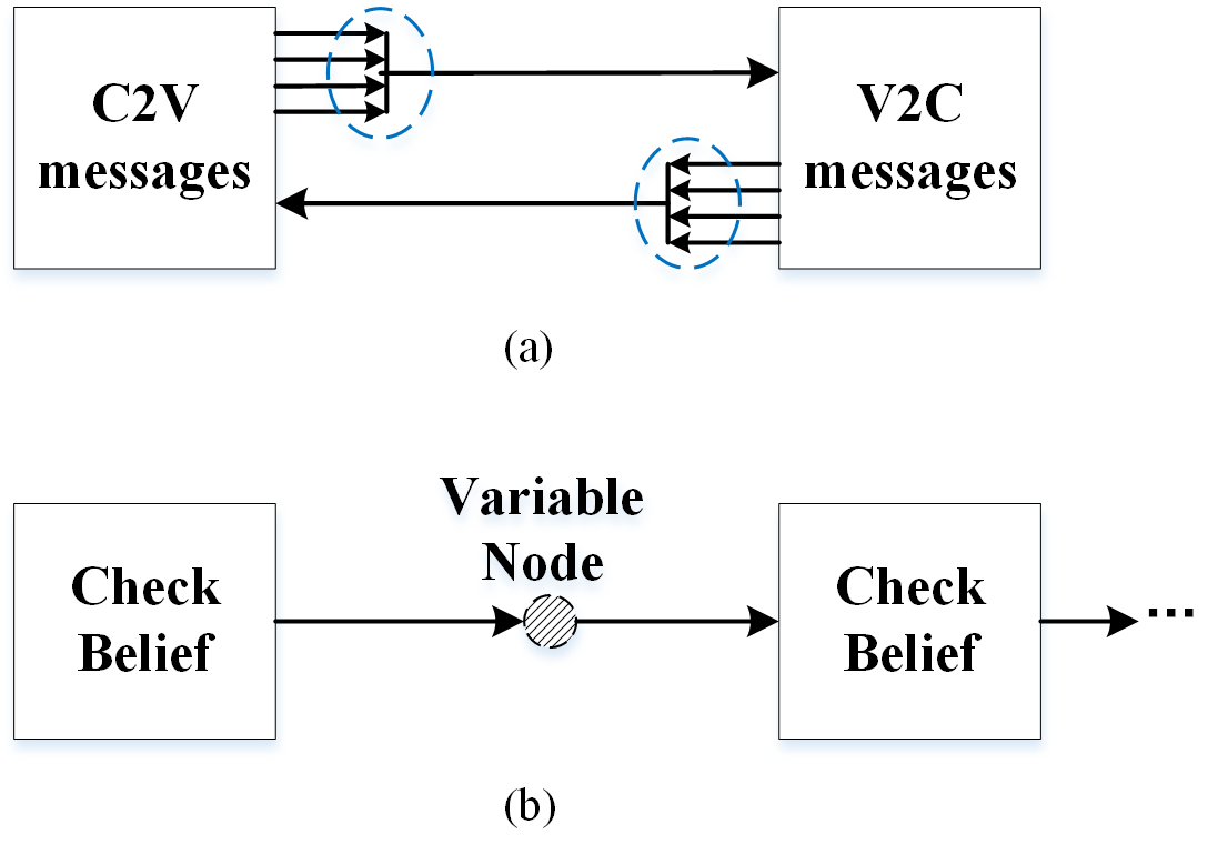
Figure 1: Message update methods of the previous algorithms and the CBP algorithm. (a) The previous algorithms gather messages from all the neighbor nodes through cumulative calculations. (b) The CBP algorithm renews check-belief from one check-node to another through only one variable-node with no cumulative calculations.

To further reduce the complexity, LDPC decoding with no cumulative calculations has been studied. As shown in Fig. 1(b), each check-belief propagates between two check-nodes through only on variable-node. The CBP decoding updates the check-beliefs serially. Compared to other algorithms gathering messages from all the neighbor nodes, CBP decoding renews each check-belief through only two other nodes. This makes that there are no cumulative calculations in CBP. It results in reducing calculations and memories for in-row/in-column message scheduling, and earns a low complexity decoding. Simulation results show that the CBP algorithm has little performance loss in contrast with the previous introduced algorithms. The analyses show that CBP consumes only one in hundreds of the calculation resources of RBP, SVNF-RBP and CI-RBP, much less calculation resources than FBP and LBP. Meanwhile, compared with the previous algorithms, it can reduce a large number of registers. Altogether, it has a much lower complexity than the above mentioned algorithms, making it suitable for high-throughput applications.

The rest of this paper is organized as follows. Section II reviews the FBP, LBP and RBP scheduling algorithms. Section III analyses the influence of cumulative calculations in variant BP decoding. Section IV proposes the CBP decoding algorithm. The error-rate performance and complexity of the CBP algorithm are investigated in Section V. Finally, Section VI concludes this paper.

II Preliminaries

A binary $(N,K)$ LDPC code $C$ with rate $R=K/N$ is characterized by a code graph $\mathbf{G}=(\mathbf{V},\mathbf{C},\mathbf{E})$, where $\mathbf{V}$, $\mathbf{C}$ and $\mathbf{E}$ are the set of variable-nodes, check-nodes and edges, respectively. There are $N$ variable-nodes in $\mathbf{V}$ and $M=N-K$ check-nodes in $\mathbf{C}$. Let $N(v)$ and $N(c)$ denote the neighbour check-nodes of variable-node $v$ and neighbour variable-nodes of check-node $c$, respectively. The symbols $N(v)\backslash c$ and $N(c)\backslash v$ denote the set $N(v)$ except for check-node $c$ and the set $N(c)$ except for variable-node $v$, respectively. Its degree distributions are represented by $(\lambda(x)=\sum_{i}\lambda_{i}x^{i-1},\rho(x)=\sum_{j}\rho_{j}x^{j-1})$, where $\lambda_{i}$ and $\rho_{j}$ denote the percentages of edges with degrees $d_{v}^{i}$ and $d_{c}^{j}$, respectively. The total number of edges in $\mathbf{E}$ is $E=N/(\sum_{i}\lambda_{i}/i)=M/(\sum_{j}\rho_{j}/j)$. Let $\mathbf{X}=[x_{v}]$ and $\mathbf{Y}=[y_{v}]$ be the code transmitted and signal received, respectively.

II-A FBP decoding

The FBP algorithm provides full parallel decoding for LDPC codes [2]. In the decoding, the V2C message sent from variable-node $v_{a}$ to check-node $c_{i}$ is updated as follows,

$$Q_{v_{a}\rightarrow c_{i}}=L_{v_{a}}+\sum_{c_{j}\in N(v_{a})\backslash c_{i}}R_{c_{j}\rightarrow v_{a}}$$ (1)

The C2V message sent from check-node $c_{i}$ to variable-node $v_{a}$ is calculated by

$$R_{c_{i}\rightarrow v_{a}}\!=\!\prod_{v_{b}\in N(c_{i})\backslash v_{a}}\!\text{sgn}\left(Q_{v_{b}\rightarrow c_{i}}\right)\!\phi\left(\sum_{v_{b}\in N(c_{i})\backslash v_{a}}\phi\left(\left|Q_{v_{b}\rightarrow c_{i}}\right|\right)\right)$$ (2)

where

$$\phi(x)=-\log\left(\tanh\frac{x}{2}\right)$$ (3)

The posterior information for each variable-node $v_{a}\in\mathbf{V}$

$$\Lambda_{v_{a}}=L_{v_{a}}+\sum_{c_{j}\in N(v_{a})}R_{c_{j}\rightarrow v_{a}}$$ (4)

is used to make tentative decision $\hat{\mathbf{X}}=[\hat{x}_{v_{a}}]$, where

$$\hat{x}_{v_{a}}=\begin{cases}0,&\Lambda_{v_{a}}\geq 0\\ 1,&\Lambda_{v_{a}}<0\\ \end{cases}$$ (5)

From the above algorithm, we can see that FBP schedules all the V2C updates using (1) in the first phase and all the C2V updates using (2) in the second phase. Therefore, in each iteration, each edge transfers its extrinsic message to its neighbours in each update. This results in a full parallel but slow-message-transfer strategy.

II-B LBP decoding

Different from the full parallel updating in FBP, LBP decoding splits each iteration into multiple propagation layers. This results in deep layer-by-layer message propagation in each iteration and hence promotes convergence.

In each layer, the V2C message is derived from the posterior information as

$$Q_{v_{a}\rightarrow c_{i}}=\Lambda_{v_{a}}-R_{c_{i}\rightarrow v_{a}}$$ (6)

and the posterior information generated from the renewed C2V messages is

$$\Lambda^{new}_{v_{a}}=Q_{v_{a}\rightarrow c_{i}}+R^{new}_{c_{i}\rightarrow v_{a}}$$ (7)

In LBP decoders, each node updates its message using all its renewed neighbours and propagates its newest message to others in each iteration. This promotes the depth of message exchange in each iteration and hence speeds up convergence.

II-C RBP decoding

To improve convergence, RBP dynamically schedules the message with the maximum C2V residuals to be updated [14]. This results in an edge-by-edge update process.

The C2V residual is generated by the magnitude difference between the current C2V message $R_{c_{i}\rightarrow v_{a}}$ and the precomputed message $R_{c_{i}\rightarrow v_{a}}^{pre}$. The C2V messages $R_{c_{i}\rightarrow v_{a}}^{pre}$ are precomputed by (2) for all the edges, and the corresponding C2V message residuals are generated by

$$r_{c_{i}\rightarrow v_{a}}=|R_{c_{i}\rightarrow v_{a}}^{pre}-R_{c_{i}\rightarrow v_{a}}|$$ (8)

The RBP schedules the edge with the maximum C2V residual to be updated, and each updated C2V message is propagated to its neighbours. In this way, the factor for check-node updates is promoted from all the neighbours’ renewal of LBP to every neighbour’s renewal in RBP, which results in a more frequent message exchange and significantly increases the convergence speed. Other methods, including NW-RBP, SVNF-RBP and CI-RBP, can also improve convergence based on reliability-based scheduling.

III Influence of Cumulative Calculations in Decoding

III-A Sole Edge Scheduling

Sole edge scheduling is usually used in informed dynamic strategies for reliability-based BP decoding, such as RBP, SVNF-RBP and CI-RBP. In this type of decoding, message updating is scheduled in an edge-by-edge manner. Each schedule updates the sole C2V message. Both V2C and C2V updates gather messages from all the neighbours; thus, their calculations are based on the cumulative sum or cumulative product of their neighbours’ messages, as described in (1) and (2). Therefore, the calculation complexity of each update is $d_{v}^{i}-1$ for the V2C message updating of a variable-node with degree $d_{v}^{i}$, and $d_{c}^{j}-1$ for the C2V message updating of a check-node with degree $d_{c}^{j}$. As $d_{v}^{i}-1$ and $d_{c}^{j}-1$ are no less than one, it results in a large complexity increase. Therefore, the sole edge scheduling, such as RBP, SVNF-RBP and CI-RBP decoding, is not a popular method for high-throughput applications.

III-B Row/Column Scheduling

Row scheduling or column scheduling, such as FBP and LBP, are popular methods for low-complexity BP decoding. In these methods, the message updating in (1) and (2) are updated as follows:

$$Q_{v_{a}\rightarrow c_{i}}=\left[L_{v_{a}}+\sum_{c_{j}\in N(v_{a})}R_{c_{j}\rightarrow v_{a}}\right]-R_{c_{i}\rightarrow v_{a}}$$ (9)

$$\begin{split}R_{c_{i}\rightarrow v_{a}}=&\left[\prod_{v_{b}\in N(c_{i})}\text{sgn}\left(Q_{v_{b}\rightarrow c_{i}}\right)\right]\cdot\text{sgn}\left(Q_{v_{a}\rightarrow c_{i}}\right)\\ &\cdot\phi\left(\left[\sum_{v_{b}\in N(c_{i})}\phi\left(\left|Q_{v_{b}\rightarrow c_{i}}\right|\right)\right]-\phi\left(\left|Q_{v_{a}\rightarrow c_{i}}\right|\right)\right)\end{split}$$ (10)

In this updating process, the values in $[\cdot]$ are shared. This means that for each variable-node $v_{a}\in N(c_{i})$, the message updating of $Q_{v_{a}\rightarrow c_{i}}$ for all $c_{i}\in N(v_{a})$ uses a shared sum $[L_{v_{a}}+\sum_{c_{j}\in N(v_{a})}R_{c_{j}\rightarrow v_{a}}]$. Similarly, a shared product is applied in the check-node processing, as shown in (10). The output value is obtained from the cumulative result exclusive of the original message.

In this updating, besides the conventional accumulative calculation for the shared value, an additional in-row/in-column scheduling process is needed to provide the original messages for the exclusive operation, as shown in Fig. 2. The shared cumulative value in $[\cdot]$ can be generated recursively, and the in-row/in-column scheduling process is used to reserve the original messages and dispatch them serially when the shared value is generated. This structure can renew one extrinsic message in each unit time. It can obtain the highest throughput among the previous various decoding methods [17].

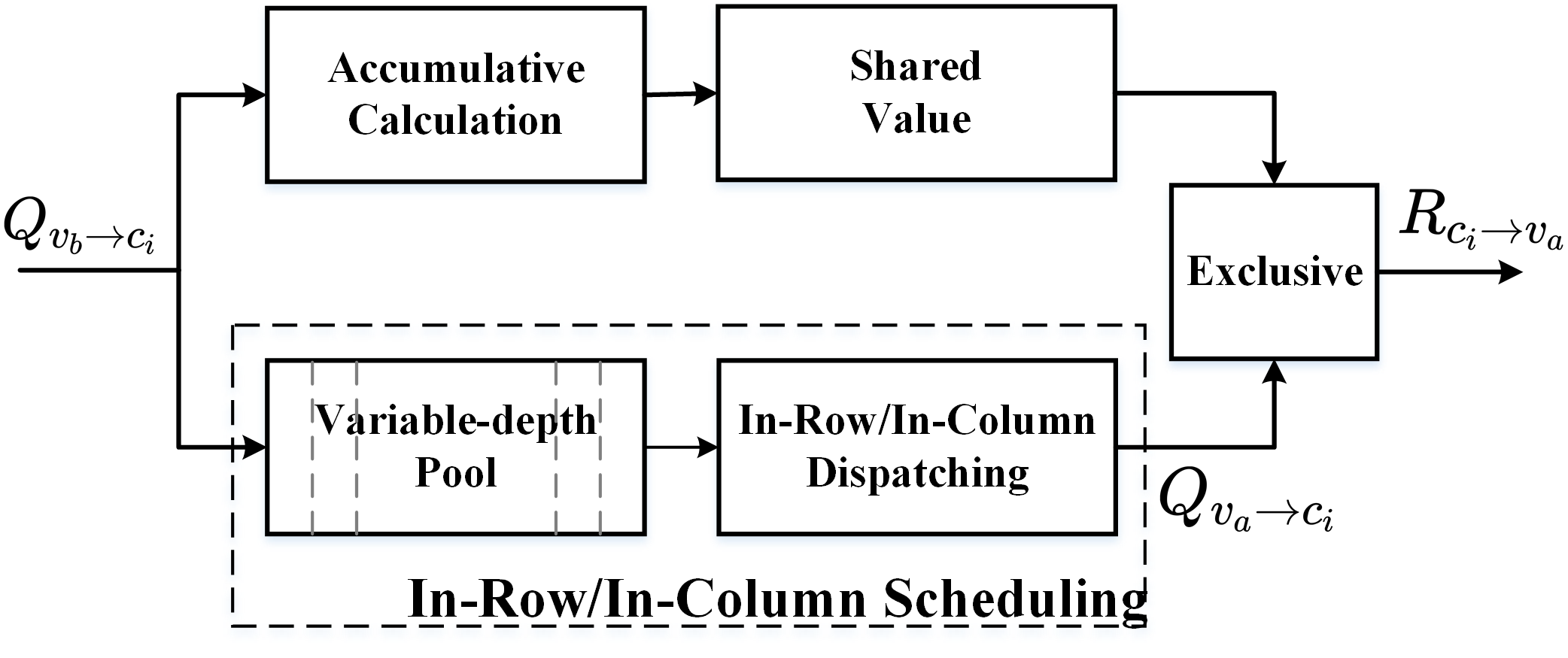
Figure 2: In-row/in-column scheduling for cumulative calculations.

However, the in-row/in-column message scheduling consumes a large number of resources. First, a pool is needed for reserving the $d_{v}^{i}$ or $d_{c}^{j}$ messages. As the degrees of reserving messages varies in a wide range, the pool depth should be a variable. It should be pointed out that a variable-depth memory cell (i.e. register) takes up to 10 to 20 times area of a general memory cell to realize its variable-connections [18]. The pool would consume many resources. Secondly, dispatching process is needed to select the original messages for the exclusive operation. Thirdly, a large number of in-row/in-column scheduling processes should be needed for parallel message updates in high-throughput applications.

As discussed above, the cumulative calculations are highly complex, either from a large number of distributed calculations in the sole edge scheduling or from a large amount of resource consumption for the in-row/in-column scheduling. Moreover, a large number of cumulative calculations consume a large number of registers. It would take 10 to 20 times area of general memories. This is a very critical drawback for high-throughput systems. The aim of non-cumulative calculation algorithms is to decrease the complexity of LDPC decoding.

IV check-belief Propagation Decoding

IV-A Check-beliefs Indicate the Probability of Successful Decoding

In conventional decoding, the V2C and C2V messages are generated with the cumulative calculations of the neighbouring nodes’ messages. This causes the problem of complexity enlargement.

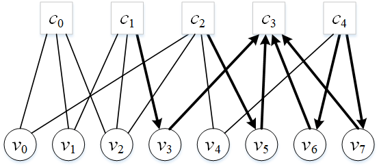
Figure 3: check-beliefs transferred from other check-nodes.

To avoid this problem, we decode the code with message exchanges between the check-nodes. Here, the check-belief of the check-node is denoted as follows [19]:

$$\Omega_{c_{i}}=\log\left(\frac{Pr(S_{c_{i}}=0|\mathbf{Y})}{Pr(S_{c_{i}}=1|\mathbf{Y})}\right)$$ (11)

where $S_{c_{i}}$ denotes the parity check corresponding to check-node $c_{i}$.

The check-belief denotes the probability that the parity check of the check-node is satisfied. For a satisfied parity check, the check-belief should be a positive value; otherwise, it should be a negative value. Thus, for successful decoding, check-beliefs for all check-nodes should be positive, that is,

$$\Omega_{c_{i}}>0,\forall c_{i}\in\mathbf{C}$$ (12)

The check-beliefs can be propagated. As shown in Fig.3, in the code graph, the check-beliefs transferred to check-node $c_{3}$ are from check-node $c_{1}$ through $v_{3}$, from check-node $c_{2}$ through $v_{5}$, from check-node $c_{4}$ through $v_{6}$ and from check-node $c_{4}$ through $v_{7}$. Therefore, the check-belief updating of check-node $c_{3}$ is based on the check-beliefs of check-nodes $c_{1}$, $c_{2}$ and $c_{4}$. Each check-node can receive several check-beliefs from the other check-nodes. This can help the check-node to increase its check-belief. By iteratively propagating the check-beliefs among the code graphs, all the check-beliefs for the check-nodes can be promoted to positive values, and thus successful decoding is achieved.

IV-B Check-Node to Check-Node Check-Belief Propagation

check-beliefs propagate from one check-node to other check-nodes through variable-nodes. They can be generated as follows [2]:

$$\Omega_{c_{i}}=\prod_{v_{a}\in N(c_{i})}\text{sgn}\left(Q_{v_{a}\rightarrow c_{i}}\right)\cdot\phi\left(\sum_{v_{a}\in N(c_{i})}\phi\left(\left|Q_{v_{a}\rightarrow c_{i}}\right|\right)\right)$$ (13)

According to the definition in (13), for every new check-node, its check-belief $\Omega_{c_{i}}^{new}$ can be updated by renewing each of its V2C messages $Q^{new}_{v_{a}\rightarrow c_{i}}$ from its neighbouring variable-nodes as follows,

$$\Omega_{c_{i}}^{new}=\prod_{v_{a}\in N(c_{i})}\text{sgn}\left(Q_{v_{a}\rightarrow c_{i}}^{new}\right)\cdot\phi\left(\sum_{v_{a}\in N(c_{i})}\phi\left(\left|Q_{v_{a}\rightarrow c_{i}}^{new}\right|\right)\right)$$ (14)

As proven in Appendix A, the check-belief in (14) can also be calculated in a recursive manner, that is,

$$\Omega_{c_{i}}^{(n)}=\psi^{+}\left(\Omega_{c_{i}}^{(n-1)},Q_{v_{a_{n}}\rightarrow c_{i}}^{new}\right)$$ (15)

where $n=0,1,\cdots,|N(c_{i})|-1$, $|N(c_{i})|$ is the number of elements in set $N(c_{i})$, and

$$\psi^{+}(x,y)=\text{sgn}(x)\cdot\text{sgn}(y)\cdot\phi\left(\phi(|x|)+\phi(|y|)\right)$$ (16)

Here, $\Omega_{c_{i}}^{(-1)}$ is initialized as $\Omega_{c_{i}}^{(-1)}=\infty$ and

$$\Omega_{c_{i}}^{new}=\Omega_{c_{i}}^{(\left|N(c_{i})\right|-1)}$$ (17)

As calculated in (6), the extrinsic V2C message $Q^{new}_{v_{a}\rightarrow c_{i}}$ can be obtained from the posterior information exclusive to the prior C2V message through variable-node $v_{a}$ as follows:

$$Q^{new}_{v_{a}\rightarrow c_{i}}=\Lambda_{v_{a}}^{new}-R_{c_{i}\rightarrow v_{a}}$$ (18)

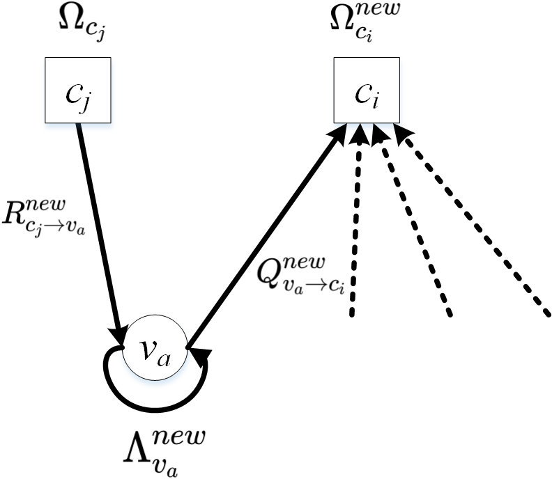
Figure 4: Check-node to check-node check-belief propagation.

Furthermore, by combining (6) and (7), we can see that the posterior information in (18) is renewed by the update of another neighbouring check-node that is different from check-node $c_{i}$, denoted as $c_{j}$. This process is given as follows:

$$\Lambda_{v_{a}}^{new}=\Lambda_{v_{a}}-R_{c_{j}\rightarrow v_{a}}+R_{c_{j}\rightarrow v_{a}}^{new}$$ (19)

The C2V message $R_{c_{j}\rightarrow v_{a}}^{new}$ in (19) can be obtained from the check-belief of $c_{j}$ by excluding its prior message following (10), that is,

$$\begin{split}R^{new}_{c_{j}\rightarrow v_{a}}=&\left[\prod_{v_{b}\in N(c_{j})}\text{sgn}\left(Q_{v_{b}\rightarrow c_{j}}\right)\right]\cdot\text{sgn}\left(Q_{v_{a}\rightarrow c_{j}}\right)\\ &\cdot\phi\left(\left[\sum_{v_{b}\in N(c_{j})}\phi\left(\left|Q_{v_{b}\rightarrow c_{j}}\right|\right)\right]-\phi\left(\left|Q_{v_{a}\rightarrow c_{j}}\right|\right)\right)\end{split}$$ (20)

As proven in Appendix A, by combining (13) and (20), we can obtain

$$R_{c_{j}\rightarrow v_{a}}^{new}=\psi^{-}\left(\Omega_{c_{j}},Q_{v_{a}\rightarrow c_{j}}\right)$$ (21)

where

$$\psi^{-}(x,y)=\text{sgn}(x)\cdot\text{sgn}(y)\cdot\phi\left(\left|\phi(|x|)-\phi(|y|)\right|\right)$$ (22)

Here, the prior V2C message $Q_{v_{a}\rightarrow c_{j}}$ is obtained from the original posterior information following (6), that is,

$$Q_{v_{a}\rightarrow c_{j}}=\Lambda_{v_{a}}-R_{c_{j}\rightarrow v_{a}}$$ (23)

The above check-belief updating process is shown in Fig.4. In this process, first, with the original check-belief $\Omega_{c_{j}}$ of check-node $c_{j}$, we can update the C2V message $R^{new}_{c_{j}\rightarrow v_{a}}$ by (20). Second, the corresponding posterior information $\Lambda^{new}_{v_{a}}$ of variable-node $v_{a}$ is updated by (19). Third, the variable-node $v_{a}$ sends a new V2C message $Q^{new}_{v_{a}\rightarrow c_{i}}$ to check-node $c_{i}$, as described by (18). Finally, check-node $c_{i}$ updates its check-belief $\Omega_{c_{i}}^{new}$ in a recursive manner, following (15). In this way, check-node $c_{j}$ transfers its check-belief $\Omega_{c_{j}}$ to check-node $c_{i}$ through variable-node $v_{a}$. This process provides a way to exchange the check-beliefs between the check-nodes, which can promote the reliability of the check-beliefs, ensuring successful decoding.

IV-C Check-belief Propagation Decoding

Here, there are usually more than two neighbouring check-nodes connected to variable-node $v_{a}$. Thus, there are multiple check-beliefs transferred from the same variable-node, as shown in Fig.5. In this code, to update the check-belief $\Omega_{c_{i}}$ of check-node $c_{i}$ through $v_{a}$, there are two candidate check-nodes $c_{j}$ and $c_{k}$. Therefore, there are two candidate check-beliefs $\Omega_{c_{j}}$ and $\Omega_{c_{k}}$, which can both transfer their check-beliefs to check-node $c_{i}$ through variable-node $v_{a}$. For good message propagation, we transfer the check-beliefs in a sequential manner. As shown in Fig.5, firstly, the check-belief $\Omega_{c_{k}}$ is transferred to check-node $c_{j}$ through variable-node $v_{a}$, and new check-belief $\Omega^{new}_{c_{j}}$ is generated. Then, the new check-belief $\Omega^{new}_{c_{j}}$ is used as prior information $\Omega_{c_{j}}$, and transferred to check-node $c_{i}$ to generate the check-belief $\Omega^{new}_{c_{i}}$. In this way, the check-beliefs are sequentially updated.

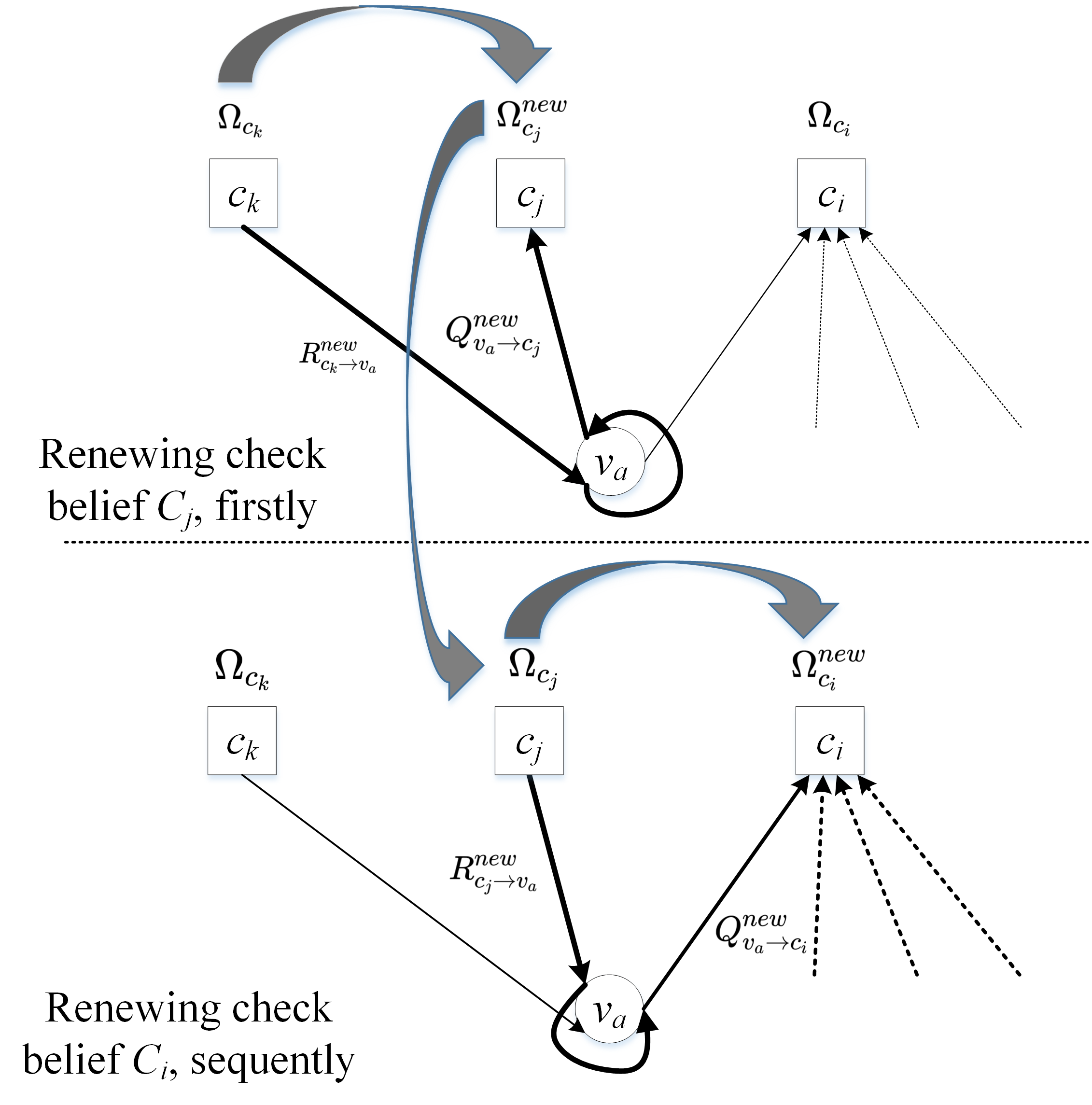
Figure 5: Sequentially check-belief propagation decoding.

From the above analysis, we can see that in sequential decoding, each check-belief $\Omega_{c_{j}}$ of check-node $c_{j}$ is used to update the check-belief of the nearest check-node $c_{i}$. Conversely, the check-belief of check-node $c_{i}$ is updated by the latest check-beliefs through its neighbouring variable-nodes. This means that for each neighbouring variable-node $v_{a}$ of check-node $c_{i}$, there are several neighbouring check-nodes $c_{k},\cdots,c_{j}$, and thus they correspond to the $N(v_{a})$ V2C messages $R_{c_{k}\rightarrow v_{a}},\cdots,R_{c_{j}\rightarrow v_{a}}$. For effective updating of the check-belief $\Omega_{c_{i}}$ through variable-node $v_{a}$, the latest check-belief $\Omega_{c_{j}}$ is used for sequential updating. The newest extrinsic information is propagated from this check-belief to other nodes, which results in improving the convergence speed for sequential decoding.

Meanwhile, only the latest V2C message is used in the sequential decoding. Thus, all the latest V2C messages can be denoted by the same symbol, $Q_{v_{a}\rightarrow c^{*}}$.

In this way, the CBP decoding algorithm can be described as follows.

• Step 1: Initialization.

For each variable-node $v_{a}\in\mathbf{V}$, the latest V2C message is

$$Q_{v_{a}\rightarrow c^{*}}=\ln\frac{Pr(y_{v_{a}}|x_{v_{a}}=0)}{Pr(y_{v_{a}}|x_{v_{a}}=1)}$$ (24)

For each check-node $c_{i}$, the check-belief is

$$\Omega_{c_{i}}=\infty$$ (25)

For each edge connected from check-node $c_{i}$ to variable-node $v_{a}$, the C2V message is

$$R_{c_{i}\rightarrow v_{a}}=0$$ (26)

Initialize the first check-node as the latest updated one.

• Step 2: Sequentially check the belief update.

For each check-node $c_{i}$, update its check-belief recursively.

(1) check-node to check-node check-belief propagation.

a) For each neighbouring variable-node $v_{a}\in N(c_{i})$, the latest updated neighbouring check-node of variable-node $v_{a}$ is denoted as $c_{j}$.

b) Check-belief to variable-node (B2V) message updating following (21),

$$R_{c_{j}\rightarrow v_{a}}^{new}=\psi^{-}\left(\Omega_{c_{j}},Q_{v_{a}\rightarrow c^{*}}\right)$$ (27)

c) V2C message updating. By combining (18), (19) and (23), the V2C message is as follows:

$$Q_{v_{a}\rightarrow c^{*}}^{new}=Q_{v_{a}\rightarrow c^{*}}+R^{new}_{c_{j}\rightarrow v_{a}}-R_{c_{i}\rightarrow v_{a}}$$ (28)

Meanwhile, according to (19) and (23), the posterior information update is generated as

$$\Lambda^{new}_{v_{a}}=Q_{v_{a}\rightarrow c^{*}}+R^{new}_{c_{j}\rightarrow v_{a}}$$ (29)

It is one part of V2C message updating. Following (29), the hard decision $\hat{x}_{v_{a}}$ can be obtained by (5).

d) Following (15), V2C message to check-belief (C2B) updating is as follows,

$$\Omega_{c_{i}}^{(n)}=\psi^{+}\left(\Omega_{c_{i}}^{(n-1)},Q_{v_{a}\rightarrow c^{*}}^{new}\right)$$ (30)

where $\Omega_{c_{i}}^{-1}=\infty$ and $\Omega_{c_{i}}^{new}=\Omega_{c_{i}}^{|N(c_{i})|-1}$.

e) Update the corresponding updated messages for check-node $c_{i}$ and variable-node $v_{a}$ as follows.

$$\begin{array}[]{ccc}R_{c_{i}\rightarrow v_{a}}&\leftarrow&R_{c_{i}\rightarrow v_{a}}^{new}\\ Q_{v_{a}\rightarrow c^{*}}&\leftarrow&Q_{v_{a}\rightarrow c^{*}}^{new}\\ \end{array}$$ (31)

This means that the renewed messages in the updating of check-node $c_{i}$ are used as prior information for the updating of the next check-node. This results in sequential decoding.

(2) The updated check-belief is renewed as a prior belief as follows:

$$\Omega_{c_{i}}\leftarrow\Omega_{c_{i}}^{new}$$ (32)

(3) Stopping criterion test.

If all the $N$ consecutive check-beliefs satisfy (12) and the posterior information signs in (29) have no flips in the $N$ consecutive check-belief updates, the decoding succeeds, that is,

$$\text{sgn}(\Lambda_{v_{a}}^{new})=\text{sgn}(\Lambda_{v_{a}})$$ (33)

Otherwise, go back to Step 2 until the maximum number of iterations is reached.

• Step 3: Output the hard decision $\hat{\mathbf{X}}=[\hat{x}_{v_{a}}]$ generated in the V2C phase of Step 2.

During decoding, each check-belief are transferred through B2V, V2C and C2B phases, following (27), (28) and (30), respectively. In this way, each check-belief can be transferred from one check-node to another check-node through only one variable-node. All the check-beliefs are iteratively enlarged in a sequential recursive order to ensure that all the parity checks are successfully satisfied. Different from previous algorithms, each check-belief is propagated through two other nodes with no cumulative calculations, which results in low complexity decoding with little performance loss.

IV-D Straightforward Decoding Structure with No Cumulative Calculations

The straightforward decoding structure is shown in Fig.6. The check-beliefs $\Omega_{c_{i}}$ for all the check-nodes, the latest V2C messages $Q_{v_{a}\rightarrow c^{*}}$ for all variable-nodes and the C2V messages $R_{c_{i}\rightarrow v_{a}}$ for all the edges in the code graph are retained in each iteration.

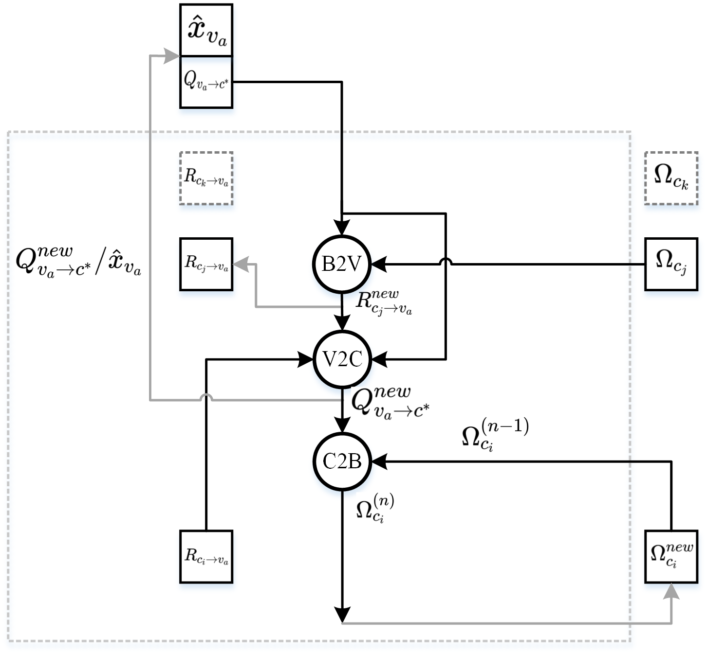
Figure 6: No cumulative calculation decoding structure for CBP decoding.

In decoding, there are three phases: the B2V, V2C and C2B phases. Firstly, in the B2V phase, the check-belief $\Omega_{c_{j}}$ and the latest V2C message $Q_{v_{a}\rightarrow c^{*}}$ are collected, and the updated C2V message $R^{new}_{c_{j}\rightarrow v_{a}}$ is generated according to (27). Secondly, in the V2C phase, the prior V2C message $Q_{v_{a}\rightarrow c^{*}}$, the prior C2V message $R_{c_{i}\rightarrow v_{a}}$ and the updated C2V message $R^{new}_{c_{j}\rightarrow v_{a}}$ are gathered, and the updating message $Q^{new}_{v_{a}\rightarrow c^{*}}$ is generated following (28). Specifically, the decision of the variable-node, $\hat{x}_{v_{a}}$, can also be decided in this step. Thirdly, in the C2B phase, the check-belief is updated recursively using the renewed V2C messages $Q^{new}_{v_{a}\rightarrow c^{*}}$.

Here, we can see that there are no cumulative calculations in the three phases. The three phases can be conducted in a straight pipeline. This results in a low-complexity decoding structure. Meanwhile, messages are transferred by two edges in each check-belief renewing. This promotes the message propagation depth and results in a high convergence speed.

Furthermore, the B2V update in (27) and C2B update in (30) can be simplified based on a normalized min-sum approach:

$$R_{c_{j}\rightarrow v_{a}}^{new}=\left(\Omega_{c_{j}}^{min}==Q_{v_{a}\rightarrow c^{*}}\right)?\Omega_{c_{j}}^{submin}:\Omega_{c_{j}}^{min}$$ (34)

$$\begin{array}[]{l}if\left(Q_{v_{a}\rightarrow c^{*}}^{new}<\Omega_{c_{i}}^{min}\right)\\ \quad\quad\left(\Omega_{c_{i}}^{min},\Omega_{c_{i}}^{submin}\right)=\left(\alpha\cdot Q_{v_{a}\rightarrow c^{*}}^{new},\Omega_{c_{i}}^{min}\right)\\ elseif\left(Q_{v_{a}\rightarrow c^{*}}^{new}<\Omega_{c_{i}}^{submin}\right)\\ \quad\quad\left(\Omega_{c_{i}}^{min},\Omega_{c_{i}}^{submin}\right)=\left(\Omega_{c_{i}}^{min},\alpha\cdot Q_{v_{a}\rightarrow c^{*}}^{new}\right)\\ end\end{array}$$ (35)

where $\Omega_{c_{i}}^{min}$ and $\Omega_{c_{i}}^{submin}$ are the minimum and the sub-minimum value of the min-sum approximation, and $\alpha$ is the normalized parameter [7].

In this way, CBP decoding can be implemented by min and sum functions instead of the log-tanh functions, making it suitable for hardware implementation.

V Performance Simulation and Complexity Analysis

We compare the performance of the traditional algorithms and the proposed CBP algorithm through the binary phase shift keying (BPSK) modulated additive white Gaussian noise (AWGN) channel. Comparisons are made for the regular (3,6) LDPC codes and irregular LDPC codes under degree distributions ($\lambda(x)=0.45x^{1}+0.3708x^{2}+0.0307x^{3}+0.1485x^{11}$, $\rho(x)=0.5467x^{4}+0.4533x^{5}$). The parity-check matrices of the LDPC codes are constructed using the progress edge growth (PEG) algorithm [20]. The codes simulated are all rate-1/2 LDPC codes. The maximum number of iterations is 200.

V-A Error Correction Performance

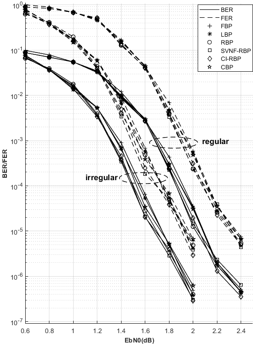
(a)

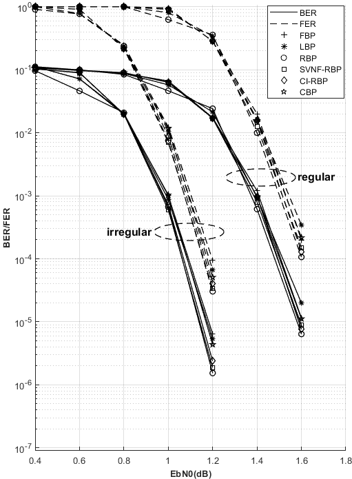
(b)

Figure 7: Performance comparisons of the FBP, LBP, RBP, SVNF-RBP, CI-RBP and the proposed CBP scheduling strategies. (a) Length-2048 LDPC codes. (b) Length-8192 LDPC codes.

Fig.7 show the AWGN performance of the FBP, LBP, RBP, SVNF-RBP, CI-RBP scheduling strategies discussed above and the proposed CBP strategy for regular and irregular LDPC codes, respectively. The figures show that the proposed CBP has a comparable performance to the other algorithms. As indicated in Fig.7, the performance differences for FBP, LBP, RBP, SVNF-RBP, CI-RBP and CBP are less than 0.05 dB for the same code. This is because these decoding algorithms all use belief propagation decoding. They use different scheduling order with different message propagation depth. This can cause different convergence speeds. However, the extrinsic information is all generated from the same parity-checks. Thus, they have similar error-correcting performances. On the other hand, RBP, SVNF-RBP and CI-RBP can schedule the flipped nodes firstly. This would decrease the influence of trapping sets, and win a performance improvement [15]. Especially, CI-RBP can conditionally schedule the flipped variable-nodes to control the influence of trapping sets, it owns much better performance than others[16].

Meanwhile, the performance and convergence comparisons for CBP decoding and its normalized min-sum approach are shown in Fig. 8 and Fig. 9. As shown in these figures, the performance loss between the normalized min-sum approach and the above log-tanh-based CBP is less than 0.2dB, and the number of iterations in the normalized min-sum approach is much larger than that of the CBP in the waterfall area and are almost the same in the low-error-rate area. This is because CBP uses log-tanh function to accurately calculate the messages during decoding, but the normalized min-sum approach uses a normalized-min function to approximate the log-tanh function. Thus, a little performance loss is observed when using the normalize min-sum method. However, it can approximate the log-tanh function in CBP with a very small deviation. Thus, both approaches have almost the same number of iterations in the low-error rate area. Thereby, the normalized min-sum approach of CBP is very suitable for hardware implementation.

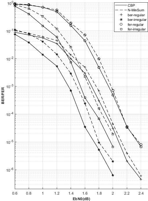
(a)

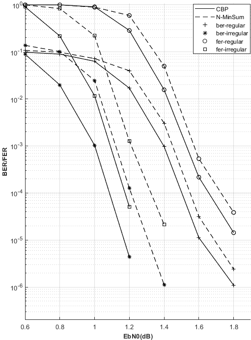
(b)

Figure 8: Performance comparisons of the CBP and its normalized min-sum approach. (a) Length-2048 LDPC codes. (b) Length-8192 LDPC codes.

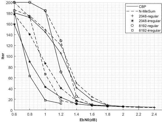
Figure 9: Iteration performance comparisons of the CBP and its normalized min-sum approach for length-2048 and length-8192 LDPC codes.

V-B Calculation Complexity

The decoding complexity of the LDPC codes includes the convergence iterations $I$, the message updates $Q$ in each iteration, and the calculations $W$ in each message update. The total complexity $T$ can be denoted as

$$T=I\times Q\times W$$ (36)

These factors will be analysed below.

V-B1 Convergence Speed

The convergence speed is measured by the average number of iterations $I$ for LDPC decoding. The simulation results for the regular and irregular codes are shown in Fig.10. From the figures above, we can see that the proposed CBP has twice the convergence speed compared to FBP, similar convergence speed as LBP, 1/2 the convergence speed compared to RBP and SVNF-RBP, and approximately 1/3 the convergence speed compared to CI-RBP. This is because the FBP exchanges messages between phases in a fully parallel manner, which results in one update for each message in each iteration. LBP and CBP exchange messages between layers in a sequential order; thus, messages can be propagated serially in columns. Thus, these approaches have better convergence speed. The RBP and SVNF-RBP approaches can improve the convergence speed through edge-by-edge updating and finish the row and column edge updating in two dimensions in each update. The CI-RBP approach can find the variable-nodes with probable incorrect decisions in RBP scheduling; thus, it has the best convergence speed.

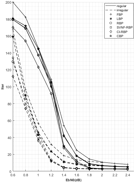
(a)

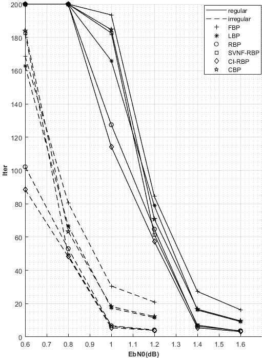
(b)

Figure 10: Convergence performance comparisons of the FBP, LBP, RBP, SVNF-RBP, CI-RBP and the proposed CBP scheduling strategies. (a) Length-2048 LDPC codes. (b) Length-8192 LDPC codes.

V-B2 Updates in Each Iteration

TABLE I: Average Updates in Each Iteration

Schedules	V2C	C2V	B2V	C2B	Residual	Comparison	Dispatching	CI
FBP	$E$	$E$	0	0	0	0	$E$	0
LBP	$E$	$E$	0	0	0	0	$E$	0
RBP	$\sum_{i}E\lambda_{i}(d_{v}^{i}-1)$	$E$	0	0	$\sum_{i,j}E\lambda_{i}\rho_{j}(d_{v}^{i}-1)(d_{c}^{j}-1)$	$E(E-1)$	0	0
SVNF-RBP	$\sum_{i}E\lambda_{i}(d_{v}^{i}-1)$	$E$	0	0	$\sum_{i,j}E\lambda_{i}\rho_{j}(d_{v}^{i}-1)(d_{c}^{j}-1)$	$E(E-1)$	0	0
CI-RBP	$\sum_{i}E\lambda_{i}(d_{v}^{i}-1)$	$E$	0	0	$\sum_{i,j}E\lambda_{i}\rho_{j}(d_{v}^{i}-1)(d_{c}^{j}-1)$	$E(E-1)$	0	$E(E-1)$
CBP	$E$	0	$E$	$E$	0	0	0	0

In Table I, the average updates of the different decoding schedules are presented. The number of updates for the FBP, LBP, RBP and SVNF-RBP schedules can be obtained from Table I in [15], while that of the CI-RBP schedule can be obtained from Table I in [16]. For each check-belief process in CBP, there are $d_{c}^{j}$ B2V updates, $d_{c}^{j}$ V2C updates and $d_{c}^{j}$ C2B updates. Thus, the numbers of B2V, V2C and C2B updates are all $\sum_{j}(E\rho_{j}/d_{c}^{j})\cdot d_{c}^{j}=E$.

V-B3 Calculations in Each Update

TABLE II: Average Calculations in Each Update

Schedules	V2C (sums)	C2V (products)	B2V (products)	C2B (products)	Residual (products)	Comparison (comparision)	Dispatching (selection)	CI (products)
FBP	2	2	0	0	0	0	$max(d_{v}^{i}$, $d_{c}^{j})$	0
LBP	2	2	0	0	0	0	$max(d_{c}^{j})$	0
RBP	$(d_{v}^{i}-1)$	$(d_{c}^{j}-1)$	0	0	$(d_{c}^{j}-1)$	1	0	0
SVNF-RBP	$(d_{v}^{i}-1)$	$(d_{c}^{j}-1)$	0	0	$(d_{c}^{j}-1)$	1	0	0
CI-RBP	$(d_{v}^{i}-1)$	$(d_{c}^{j}-1)$	0	0	$(d_{c}^{j}-1)$	1	0	2
CBP	2	0	1	1	0	0	0	0

In Table II, the average numbers of calculations for each update of FBP, LBP, RBP, SVNF-RBP, CI-RBP and the proposed CBP strategies are presented. The numbers of sums and products in the V2C updates, C2V updates and precomputation are the node degree minus one in RBP, SVNF-RBP and CI-RBP. However, the numbers of V2C updates and C2V updates are all two because they can be carried out in a row or column scheduling manner. Unfortunately, they need an additional in-row/in-column scheduling process for reserving and dispatching the original messages. Furthermore, in CBP, as described in Algorithm 1, there is one product for the B2V update, two sums (including substrates) for the V2C update and one product for the C2B update. Specifically, in CI-RBP, there are exponential functions and division operations, which are no less than two products.

V-B4 Total Complexity

To determine the total complexity, we set the convergence speeds as 1, 1/2, 1/2, 1/4, 1/4 and 1/6 for FBP, LBP, CBP, RBP, SVNF-RBP and CI-RBP, respectively, as discussed above. By combining the convergence speed and data in Table I and Table II, the total number of calculations in each iteration is determined and shown in Table III.

TABLE III: Total Complexity

Schedules	Sums	Products	Comparison	Selection
FBP	$2E$	$2E$	0	$E\cdot max(d_{v}^{i},d_{c}^{j})$
LBP	$E$	$E$	0	$E\cdot max(d_{c}^{j})/2$
RBP	$\sum_{i}E\lambda_{i}(d_{v}^{i}-1)^{2}/4$	$\sum_{j}E\rho_{j}(d_{c}^{j}-1)/4+$ $\sum_{i,j}E\lambda_{i}\rho_{j}(d_{v}^{i}-1)(d_{c}^{j}-1)^{2}/4$	$E(E-1)/4$	0
SVNF-RBP	$\sum_{i}E\lambda_{i}(d_{v}^{i}-1)^{2}/4$	$\sum_{j}E\rho_{j}(d_{c}^{j}-1)/4+$ $\sum_{i,j}E\lambda_{i}\rho_{j}(d_{v}^{i}-1)(d_{c}^{j}-1)^{2}/4$	$E(E-1)/4$	0
CI-RBP	$\sum_{i}E\lambda_{i}(d_{v}^{i}-1)^{2}/6$	$\sum_{j}E\rho_{j}(d_{c}^{j}-1)/6+$ $\sum_{i,j}E\lambda_{i}\rho_{j}(d_{v}^{i}-1)(d_{c}^{j}-1)^{2}/6+$ $E(E-1)/3$	$E(E-1)/6$	0
CBP	$E$	$E$	0	0

As shown in Table III, the complexity of FBP, LBP and CBP is $O(E)$, while that of RBP, SVNF-RBP and CI-RBP is $O(E^{2}/4)$. As $E$ is the number of edges, it is a very big integer. Thus, the complexity of RBP, SVNF-RBP and CI-RBP is much larger than that of CBP. Obviously, there are approximately $E$ more sums, $E$ more products and $E\cdot max(d_{v}^{i},d_{c}^{j})$ more selections for FBP than for CBP. There are $E\cdot max(d_{c}^{j})$ more selections for LBP than for CBP. Thus, the complexity of FBP and LBP is larger than that of CBP, too. Altogether CBP has the lowest calculation complexity among the previous introduced strategies.

To explicitly illustrate the comparisons, numerical results of Table III are shown in Table IV and Table V for (3,6) regular LDPC codes and the above ($\lambda(x),\rho(x)$) irregular ones, respectively. As shown in Table IV and Table V, there are $O(E^{2})$ more comparisons and $O(E)$ more products in RBP, SVNF-RBP and CI-RBP than in CBP. Meanwhile, the number of sums is much less than that of products and comparisons. As $E$ is usually more than hundreds, the complexity of RBP, SVNF-RBP and CI-RBP would be hundreds of times that of CBP. On the other hand, there are multiple of $E$ more selections, $E$ more sums and $E$ more products in FBP than in CBP, and multiple of $E$ more selections in LBP than in CBP. Thus, CBP earns a big benefit in terms of calculation complexity.

TABLE IV: Total Complexity for (3,6) LDPC Codes

Schedules	Sums	Products	Comparisons	Selections
FBP	$2E$	$2E$	0	$6E$
LBP	$E$	$E$	0	$3E$
RBP	$E$	$13.75E$	$E(E-1)/4$	0
SVNF-RBP	$E$	$13.75E$	$E(E-1)/4$	0
CI-RBP	$0.67E$	$E(E/3+8.83)$	$E(E-1)/6$	0
CBP	$E$	$E$	0	0

TABLE V: Total Complexity for the above ($\lambda(x),\rho(x)$) LDPC Codes

Schedules	Sums	Products	Comparisons	Selections
FBP	$2E$	$2E$	0	$12E$
LBP	$E$	$E$	0	$3E$
RBP	$5.04E$	$15.76E$	$E(E-1)/4$	0
SVNF-RBP	$5.04E$	$15.76E$	$E(E-1)/4$	0
CI-RBP	$3.36E$	$E(E/3+10.17)$	$E(E-1)/6$	0
CBP	$E$	$E$	0	0

V-C Memory Consumption

The memory consumed during decoding is depicted in Table VI. Specially, variable-depth pool uses registers for variable-connections while the others use general memories. As shown in Table VI, there are $2E-M$ more general cells for RBP, SVNF-RBP and CI-RBP than for CBP. There are $E-M$ more general cells and $P\cdot max(d_{v}^{i},d_{c}^{j})$ registers for FBP than for CBP. In LBP, there are $M$ less general cells, but $P\cdot max(d_{c}^{j})$ more registers than in CBP. It should be pointed out that a register (not including the mux logics) takes up to 10 to 20 times area of a general memory cell [18]. Thus, CBP owns the least memory consumption.

TABLE VI: Memory Consumption

Schedules	LLR	C2V	V2C	Residual	Check-belief	variable-depth pool
FBP	$N$	$E$	$E$	0	0	$P\cdot max(d_{v}^{i},d_{c}^{j})$
LBP	$N$	$E$	0	0	0	$P\cdot max(d_{c}^{j})$
RBP	$N$	$E$	$E$	$E$	0	0
SVNF-RBP	$N$	$E$	$E$	$E$	0	0
CI-RBP	$N$	$E$	$E$	$E$	0	0
CBP	$N$	$E$	0	0	$M$	0

Reducing the variable-depth pool can result in a large improvement. For example, for the parallel decoding of LDPC codes in 5G NR, assuming a parallel number of $P=384$, $M=46P$, the depth of the pool ranges from 3 to 19, and each message is soft quantized by 8 bits [21]. During decoding, the CBP can reduce approximately $384\times 19\times 8=58,368$ registers. Additionally, it would cost $384\times 46\times 8=141,312$ bits of general memories for reserving check-beliefs, which is equivalent to 14,131 registers. Totally, CBP would reduce about $58,368-14,131=44,237$ bits of registers, compared to other algorithms. A very large number of memory resources is saved, which will improve the cost significantly.

VI Conclusion

In this paper, we have presented an innovative strategy, CBP, based on the check-belief of each check-node. Each check-belief is propagated from one check-node to another check-node through only one variable-node in a recursive manner. This method can strengthen the check-belief sufficiently, ensuring that the corresponding parity check is satisfied and successful decoding is achieved. Compared to previous algorithms employing a large number of cumulative calculations, CBP decoding can renew messages through only two other nodes with no cumulative calculations. This results in reducing calculations and memories for in-row/in-column message scheduling, and earns a low complexity decoding. Simulation results show that the CBP algorithm has no performance loss in contrast with the previous introduced algorithms. The analyses show that CBP consumes only one in hundreds of the calculation resources of RBP, SVNF-RBP and CI-RBP, much less calculation resources than FBP and LBP. Meanwhile, compared with previous algorithms, it can reduce a large number of registers. It has a much lower complexity than the above mentioned algorithms.

[Proof of Inclusive Equations] Here, we note that $\phi(x)$ in (3) is a self-reciprocal function, that is, $\phi^{-1}(x)=\phi(x),\forall x>0$.

Define the right part of (13) as follows:

$$Y_{n}=\phi\left(\sum_{i=0}^{n-1}\phi\left(x_{i}\right)\right).$$ (37)

The inverse of (37) is

$$\phi^{-1}(Y_{n})=\sum_{i=0}^{n-1}\phi\left(x_{i}\right)$$ (38)

According to (38), we can obtain

$$\begin{split}\phi^{-1}(Y_{n+1})&=\sum_{i=0}^{n}\phi\left(\left|x_{i}\right|\right)\\ &=\phi^{-1}(Y_{n})+\phi(x_{n})\\ &=\phi(Y_{n})+\phi(x_{n})\end{split}$$ (39)

Thus,

$$Y_{n+1}=\phi\left(\phi(Y_{n})+\phi(x_{n})\right)$$ (40)

This proves the recursive function in (15).

According to (38), we can also obtain

$$\begin{split}\phi^{-1}(Y_{n-1})&=\sum_{i=0}^{n-2}\phi\left(\left|x_{i}\right|\right)\\ &=\phi^{-1}(Y_{n})-\phi(x_{n-1})\\ &=\phi(Y_{n})-\phi(x_{n-1})\end{split}$$ (41)

Thus,

$$Y_{n-1}=\phi\left(\phi(Y_{n})-\phi(x_{n-1})\right)$$ (42)

According to (38), we know that $\phi(Y_{n})>\phi(x_{n-1})$. However, the result of $\left(\phi(Y_{n})-\phi(x_{n})\right)$ would be a negative value when it is very small. Thus, we usually use (42) as follows:

$$Y_{n-1}=\phi\left(\left|\phi(Y_{n})-\phi(x_{n-1})\right|\right)$$ (43)

This proves the recursive function in (21).

References

- [1] R. G. Gallager, “Low-density parity-check codes,” IRE Trans. Inf. Theory, vol. 8, pp. 21–28, Jan. 1962.
- [2] Second Generation Framing Structure Channel Coding and Modulation Systems for Broadcasting, Digital Video Broadcasting (DVB) standard, ETSI EN 302 307, June 2004.
- [3] IEEE Draft Standard for Information Technology-Wireless LANs—Part 21: mmWave PHY Specification, IEEE Standard 802.11ad, May 2010.
- [4] Multiplexing and Channel Coding, (V 15.3.0) Release 15, 3GPP Standard, TS 38.212, Oct. 2018.
- [5] D. J. C. MacKay and R. M. Neal, “Near Shannon Limit Performance of Low Density Parity Check Codes,” Electron. Lett., vol. 32, no. 18, pp.1645-1646, Jul. 1996.
- [6] J. Zhao, F. Zarkeshvari and A. H. Banihashemi, ”On implementation of min-sum algorithm and its modifications for decoding low-density Parity-check (LDPC) codes,” IEEE Trans. Comm., vol. 53, no. 4, pp. 549-554, April 2005.
- [7] J. Chen, A. Dholakia, E. Eleftheriou, M. P. C. Fossorier and Xiao-Yu Hu, ”Reduced-complexity decoding of LDPC codes,” IEEE Trans. Comm., vol. 53, no. 8, pp. 1288-1299, Aug. 2005.
- [8] D. E. Hocevar, ”A reduced complexity decoder architecture via layered decoding of LDPC codes,” IEEE Workshop on Signal Proc. Syst., 2004. SIPS 2004., 2004, pp. 107-112.
- [9] K. Tian and H. Wang, ”A Novel Base Graph Based Static Scheduling Scheme for Layered Decoding of 5G LDPC Codes,” IEEE Comm. Lett., vol. 26, no. 7, pp. 1450-1453, July 2022.
- [10] E. Sharon, S. Litsyn and J. Goldberger, ”An efficient message-passing schedule for LDPC decoding,” 2004 23rd IEEE Convention of Electrical and Electronics Engineers in Israel, 2004, pp. 223-226.
- [11] S. Usman and M. M. Mansour, ”Fast Column Message-Passing Decoding of Low-Density Parity-Check Codes,” IEEE Trans. Circuits Syst. II: Express Briefs, vol. 68, no. 7, pp. 2389-2393, July 2021.
- [12] X. Pang, W. Song, Y. Shen, X. You and C. Zhang, ”Efficient Row-Layered Decoder for Sparse Code Multiple Access,” IEEE Trans. Circuits Syst. I: Regular Papers, vol. 68, no. 8, pp. 3495-3507, Aug. 2021.
- [13] B. S. Su, C. H. Lee and T. D. Chiueh, ”A 58.6/91.3 pJ/b Dual-Mode Belief-Propagation Decoder for LDPC and Polar Codes in the 5G Communications Standard,” IEEE Solid-State Circuits Lett., vol. 5, pp. 98-101, 2022.
- [14] A. I. V. Casado, M. Griot and R. D. Wesel, ”Informed Dynamic Scheduling for Belief-Propagation Decoding of LDPC Codes,” 2007 IEEE Int. Conf. on Comm., 2007, pp. 932-937.
- [15] H. Lee, Y. Ueng, S. Yeh and W. Weng, ”Two Informed Dynamic Scheduling Strategies for Iterative LDPC Decoders,” IEEE Trans. Comm., vol. 61, no. 3, pp. 886-896, March 2013.
- [16] T. C. Y. Chang, P. H. Wang, J. J. Weng, I. H. Lee and Y. T. Su, ”Belief-Propagation Decoding of LDPC Codes With Variable Node–Centric Dynamic Schedules,” IEEE Trans. Comm., vol. 69, no. 8, pp. 5014-5027, Aug. 2021.
- [17] Z. Wang and Z. Cui, ”A Memory Efficient Partially Parallel Decoder Architecture for Quasi-Cyclic LDPC Codes,” IEEE Trans. Very Large Scale Integration (VLSI) Systems, vol. 15, no. 4, pp. 483-488, April 2007.
- [18] K. Gaurav, R. S. Surendra, R. C. Naga, D. Sudeb, ”Radiation Hard Circuit Design: Flip-Flop and SRAM,” VLSI and Post-CMOS Electronics, Volume 2: Devices, Circuits and Interconnects, IET Digital Library, pp. 249-278.
- [19] G. B. Kyung and C. C. Wang, ”Finding the Exhaustive List of Small Fully Absorbing Sets and Designing the Corresponding Low Error-Floor Decoder,” IEEE Trans. Comm., vol. 60, no. 6, pp. 1487-1498, June 2012.
- [20] Xiao-Yu Hu, E. Eleftheriou and D. M. Arnold, ”Regular and irregular progressive edge-growth tanner graphs,” IEEE Trans. Inf. Theory, vol. 51, no. 1, pp. 386-398, Jan. 2005.
- [21] J. Nadal and A. Baghdadi, ”Parallel and Flexible 5G LDPC Decoder Architecture Targeting FPGA,” in IEEE Trans. Very Large Scale Integration (VLSI) Systems, vol. 29, no. 6, pp. 1141-1151, June 2021.