Concentration in an advection-diffusion model with diffusion coefficient depending on the past trajectory

Abstract.

We consider a drift-diffusion model, with an unknown function depending on the spatial variable and an additional structural variable, the amount of ingested lipid. The diffusion coefficient depends on this additional variable. The drift acts on this additional variable, with a power-law coefficient of the additional variable and a localization function in space. It models the dynamics of a population of macrophage cells. Lipids are located in a given region of space; when cells pass through this region, they internalize some lipids. This leads to a problem whose mathematical novelty is the dependence of the diffusion coefficient on the past trajectory. We discuss global existence and blow-up of the solution.

1. Introduction

1.1. The problem at hand

Atherosclerosis is a major cause of death in industrialized societies since it is the primary cause of heart attack (acute myocardial infarction) and stroke (cerebrovascular accident). It is now accepted that atherosclerosis is a chronic inflammatory disease which starts within the intima, the innermost layer of an artery. It is driven by the accumulation of macrophage cells within the intima and promoted by modified low density lipoprotein (LDL) particles [6, 7]. Inflammation occurs at sites within the arterial wall where modified low-density lipoproteins (LDL) accumulate after penetrating the wall from the bloodstream. The immune response attracts circulating monocytes to these sites.

Mathematical modeling of atherosclerosis has recently gained interest because of the variety of behavior of macrophages depending on the amount of lipid ingested [8]. Many mathematical models divide the macrophage population into “macrophages” and “foam cells”. This is true in models based on ordinary differential equations [12], spatially resolved partial differential equations models [13, 14, 15, 10, 11] and other computational models [17]. However, it is now clear that there is a continuous distribution of lipid loads in macrophage populations, ranging from monocytes with low lipid loads to macrophages that can be labeled as foam cells in atherosclerosis. The variation in lipid load within a macrophage population suggests that it may be instructive to develop structured models in which macrophages are characterized by their intracellular lipid load, similar to adipocytes [18], in the spirit of [9, 19].

We consider here the case where the arterial wall is $\mathbb{R}^{d}$ with $d\geq 1$ and lipids are localized in a prescribed region defined by $\operatorname*{Supp}\psi$ where $\psi$ is a given non-negative function of space. We describe the dynamics of macrophages in the arterial wall by a statistical (kinetic) description of the evolution of their density with respect to the spatial and lipid variables:

(1.1) $$\begin{cases}\partial_{t}u=a\Delta_{x}u+\partial_{a}\left\{\left[\psi(x)f(a)-\lambda a(A^{*}-a)\right]u\right\},&x\in\mathbb{R}^{d},a\geq 0,t>0,\\[5.69054pt] u_{|t=0}=u_{0},&x\in\mathbb{R}^{d},a\geq 0,\end{cases}$$

where $A^{*}>0$, $\lambda\geq 0$ and $f$ is a given function.

In (1.1), $u(t,x,a)$ is the density of cells (macrophages) located at time $t$ in $x\in\mathbb{R}^{d}$ and having with an amount $a$ of ingested lipids. The amount of lipids in the cell affects its spatial dynamics by changing its size for example. This effect is modeled by a diffusion coefficient depending on the variable $a$. The term $\lambda a(A^{*}-a)$ is a logistic (dumping) term that describes the recovery effect, i.e. the tendency of a cell to return to its normal state as it moves away from the hot spot.

We address the question of whether or not this advection-diffusion equation can lead to concentration and eventually blow-up in finite time, if diffusion is not strong enough to prevent cells from being trapped in lipid dense regions. More precisely, our purposes here are to investigate the influence of the nonlinearity $f$, the parameter $\lambda$ and the size of the support of $\psi$ on the local or global well-posedness of problem (1.1). To this end we will consider functions $f$ which typically grow like a power, namely

$$f(a)=\pm a^{\gamma}\textrm{ with }\gamma>0,$$

and three different cases for the function $\psi$:

1. $\psi=\mathds{1}_{\mathbb{R}}$,

2. $\operatorname*{Supp}\psi\left(x\right)\subset B(0,1)$ with $\int_{\mathbb{R}^{d}}\psi\left(x\right)\operatorname{d}\!x=1$,

3. $\psi=\delta_{x=0}$ is the Dirac mass in dimension $d=1$, which was treated in [5] when $\lambda=0$.

1.2. The origin of the model

Let us briefly detail the origin of equation (1.1) in the case where $d=1$, see [2, 5, 4] for more details. Consider a cell, described as a Brownian particle, with position $X_{t}$, whose diffusion coefficient, $A_{t}$, is modified at each passage in the lipid-rich zone and which tends to recover a normal diffusion coefficient, see Figure 1. The couple $(X_{t},A_{t})$ satisfies the system of stochastic differential equations

(1.2) $$\begin{cases}\operatorname{d}\!X_{t}&=\sqrt{2A_{t}}\operatorname{d}\!W_{t},\\[5.69054pt] \operatorname{d}\!A_{t}&=-\psi(X_{t})f(A_{t})\operatorname{d}\!t+\ \lambda A_{t}\left(A^{*}-A_{t}\right)\operatorname{d}\!t,\end{cases}$$

with initial condition $X_{0}\in\mathbb{R}$, $A_{0}>0$, where $(W_{t},t\geq 0)$ is a one-dimensional Brownian motion.

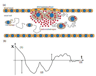
Figure 1. a) Sketch of the different stages of atherosclerosis plaque formation: (1) rapid diffusion of a “free” macrophage cell; (2) upon entering a localized lipid-enriched region, the macrophage accumulates lipids, and thereby grows and becomes less mobile; and (3) after many crossings of the lipid-enriched region, the macrophage eventually gets trapped, resulting in the formation of an atherosclerotic plaque. (b) Sketch of a one-dimensional particle trajectory of the model of locally decelerated random walk.

Intuitively, $\int_{0}^{t}\psi(X_{s})\operatorname{d}\!s$ represents the time spent by $X$ in the lipid-rich region during $[0,t]$. Hence, when $f\geq 0$, the time spent in this region by the macrophage cell tends to decrease its diffusion coefficient $(A_{t},t\geq 0)$, or equivalently to decelerate the cell. Such a decrease in local mobility is due to the internalization and accumulation of lipid particles by macrophages. It can be related to several phenomena: increase in volume or change in cell fate depending on the amount of low-density lipoproteins (LDL) ingested.

The parameter $\gamma$ describes the intensity of the internalization: the higher $\gamma$ is, the lower the internalization is. This parameter is thus related to both the amount of lipids located in the arterial wall hotspot and the capacity of macrophages to internalize lipids. The case $\gamma=0$ corresponds to a very large amount of lipids and a very large capacity of macrophages to internalize lipids. In summary, the parameter $\gamma$ is related to the inflammatory state. In contrast, the term $\lambda A_{t}\left(A^{*}-A_{t}\right)\operatorname{d}\!t$ describes the loss of lipids by the macrophage and its tendency to recover its natural state. The parameters $\lambda$ and $A^{*}$ model the natural immune defenses or medical treatment.

System (1.2) models the effects of lipid accumulation on macrophage dynamics. The novelty of (1.2), compared with the related model in [2, 5], is to include different geometries for lipid source locations (from the Dirac case to the whole real line) and to include the lipid unloading through the logistic dumping term. Non-trivial behaviors of the solution of (1.2) are expected: a dynamic transition to an absorbing state can occur for a sufficiently strong deceleration, and the particle can be trapped in finite time; whereas if the deceleration process is sufficiently weak, the particle is never trapped.

1.3. The main results

Since the couple $(X_{t},A_{t})$ is Markovian, in order to make the previous intuition rigorous, we study the partial differential equation (1.1) and the general questions we are concerned with are the following. By studying the regularity of the solution to (1.1), do we recover the results expected by the probabilistic description, in particular by the simplified differential equations $A^{\prime}(t)=-f(A(t))$? In particular, if $f(a)=a^{\gamma}$ with $\gamma\geq 1$, can we prove global existence as expected from the previous differential equation? In the case $f(a)=a^{\gamma}$ with $\gamma\in(0,1)$, can we prove that the solution to (1.1) becomes unbounded in finite time in any $L^{p}$ space? In order to ease the presentation, we will discuss the particular case of space dimension 1. However, our results remain true in dimension 2. In Section 4.3 we explain the changes in order to recover the blow-up for $\gamma\in[0,1)$ in the the two-dimensional case.

Let us build some intuition on (1.1) in the case where $f(a)=a^{\gamma}$, $\psi=\mathds{1}_{\mathbb{R}}$, $\lambda=0$ and $d=1$. Multiplying (1.1) with $a^{\gamma}$ and denoting $m(t,x,a)=a^{\gamma}u(t,x,a)$, we obtain:

(1.3) $$\partial_{t}m(t,x,a)=a\partial_{xx}m(t,x,a)+a^{\gamma}\partial_{a}m(t,x,a)\,.$$

Let us assume that $\partial_{x}m(t,x,a)$ vanishes at $x\sim\pm\infty$ and let us integrate equation (1.3) on $\mathbb{R}$:

(1.4) $$\partial_{t}\int_{\mathbb{R}}m(t,x,a)\operatorname{d}\!x-a^{\gamma}\partial_{a}\int_{\mathbb{R}}m(t,x,a)\operatorname{d}\!x=0\,.$$

We then write the characteristics $a(t)$ of the previous system, solution to the equation:

(1.5) $$\begin{cases}a^{\prime}(t)&=-a^{\gamma}(t)\\ a(0)&=a_{0}.\end{cases}$$

The equation (1.5) shows how the diffusion coefficient evolves (note that it changes in the same way for all individuals) namely we identify two different regimes:

• if $\gamma\in[0,1)$ the diffusion coefficient vanishes in finite time,

• if $\gamma\geq 1$ the diffusion coefficient is positive for all time provided the initial datum $a_{0}>0$, and vanishes asymptotically in time as $t\to+\infty$.

We are now in the position of stating our main results. We begin with the case where the acceleration-deceleration zone is the whole real axis:

(1.6) $$\begin{cases}\partial_{t}u=a\partial_{xx}^{2}u+\partial_{a}\left(f(a)u\right),&x\in\mathbb{R},\ a\geq 0,\ t>0,\\[5.69054pt] u_{|t=0}=u_{0},&x\in\mathbb{R},\ a\geq 0.\end{cases}$$

We consider the three following cases:

• acceleration: $f(a)=-a^{\gamma}$ with $\gamma\geq 0$,

• subcritical deceleration: $f(a)=a^{\gamma}$ with $\gamma\geq 1$,

• supercritical deceleration: $f(a)=a^{\gamma}$ with $\gamma\in[0,1)$.

In particular, if $f(a)=a^{\gamma}$, by studying the regularity of the solution in a $L^{p}$ framework, we obtain the following dichotomy: global existence if $\gamma\geq 1$, while, in the case $\gamma<1$, the solution becomes unbounded in finite time (so-called blow-up).

This is a linear equation on $u=u(t,x,a)$ defined on $t\geq 0$, $x\in\mathbb{R}$, $a\geq 0$.

The first main result reads :

Theorem 1.1.

Assume that the initial datum $u_{0}$ belongs to $L^{p}\cap L^{1}$, $p\geq 1$. Assume in addition that $\mbox{supp}(u_{0})\subset\mathbb{R}\times[0,A_{0}]$ for some $A_{0}>0$, then

• in the acceleration case $f(a)=-a^{\gamma}$ with $\gamma\geq 0$, there exists a unique global weak solution to (1.6) that satisfies

  $$\forall\,t\geq 0,\quad\int_{\mathbb{R}}\int_{\mathbb{R}_{+}}|u(t,x,a)|^{p}\operatorname{d}\!x\operatorname{d}\!a\leq\int_{\mathbb{R}}\int_{\mathbb{R}_{+}}|u(0,x,a)|^{p}\operatorname{d}\!x\operatorname{d}\!a,$$

• in the subcritical deceleration case $f(a)=a^{\gamma}$ with $\gamma\geq 1$, there exists a unique global weak solution to (1.6) that satisfies

  $$\forall\,t\geq 0,\quad\int_{\mathbb{R}}\int_{\mathbb{R}_{+}}|u(t,x,a)|^{p}\operatorname{d}\!x\operatorname{d}\!a\leq e^{\gamma(1-p)A_{0}^{\gamma-1}t}\int_{\mathbb{R}}\int_{\mathbb{R}_{+}}|u(0,x,a)|^{p}\operatorname{d}\!x\operatorname{d}\!a,$$

• in the supercritical deceleration case $f(a)=a^{\gamma}$ with $\gamma\in[0,1)$, any non-zero weak solution to (1.6) blows-up in finite time with the time of blow-up

  $$T_{b}:=\frac{\int_{\mathbb{R}}\int_{\mathbb{R}_{+}}a^{1-\gamma}u(0,x,a)\operatorname{d}\!x\operatorname{d}\!a}{(1-\gamma)\left(\int_{\mathbb{R}}\int_{\mathbb{R}_{+}}u(0,x,a)\operatorname{d}\!x\operatorname{d}\!a\right)}\in(0,+\infty)$$

  for which all the mass is concentrated at $a=0$.

Our second result concerns the case where the acceleration-deceleration zone is localized:

(1.7) $$\begin{cases}\partial_{t}u=a\partial_{xx}^{2}u+\psi\left(x\right)\partial_{a}\left(f(a)u\right),&x\in\mathbb{R},\ a\geq 0,\ t>0,\\[5.69054pt] u_{|t=0}=u_{0},&x\in\mathbb{R},\ a\geq 0,\end{cases}$$

with a localization function that satisfies

$$\operatorname*{Supp}\psi\left(x\right)\subset\left[-1,1\right]\quad\text{ and }\quad\int_{\mathbb{R}}\psi\left(x\right)\operatorname{d}\!x=1.$$

We will consider the three regimes described above.

Theorem 1.2.

Given $u_{0}\in L^{1}\cap L^{p}$, $p\geq 1$, with $u_{0}\geq 0$ and $\operatorname{supp}u_{0}\subset\mathbb{R}\times[0,A_{0}]$, $A_{0}>0$, we have:

• In the acceleration case, $f(a)=-a^{\gamma}$ with $\gamma>0$, there exists a unique weak solution to (3.5) that satisfies

  $$\forall\,t\geq 0,\quad\int_{\mathbb{R}}\int_{\mathbb{R}_{+}}|u(t,x,a)|^{p}\operatorname{d}\!x\operatorname{d}\!a\leq\int_{\mathbb{R}}\int_{\mathbb{R}_{+}}|u(0,x,a)|^{p}\operatorname{d}\!x\operatorname{d}\!a,.$$

• In the subcritical deceleration case $f(a)=a^{\gamma}$ with $\gamma\geq 1$, there exists a unique weak solution to (3.5) that satisfies

  $$\forall\,t\geq 0,\quad\int_{\mathbb{R}}\int_{\mathbb{R}_{+}}|u(t,x,a)|^{p}\operatorname{d}\!x\operatorname{d}\!a\leq e^{\frac{\gamma(p-1)A_{0}^{\gamma-1}}{2\delta}t}\int_{\mathbb{R}}\int_{\mathbb{R}_{+}}|u(0,x,a)|^{p}\operatorname{d}\!x\operatorname{d}\!a.$$

  Moreover, when $\gamma>3/2$, the following bound (uniform in $\delta$) holds

  $$\forall\,t\geq 0,\quad\int_{\mathbb{R}}\int_{\mathbb{R}_{+}}|u(t,x,a)|^{p}\operatorname{d}\!x\operatorname{d}\!a\leq e^{\gamma^{2}(p-1)t}\int_{\mathbb{R}}\int_{\mathbb{R}_{+}}|u(0,x,a)|^{p}\operatorname{d}\!x\operatorname{d}\!a.$$

• in the supercritical deceleration case $f(a)=a^{\gamma}$ with $\gamma\in[0,1)$, provided that $a_{0}$ is small, there exists arbitrarily small non-negative initial data

  $$0\leq u_{0}\in L^{1}\cap L^{p}(\mathbb{R}\times\mathbb{R}_{+}),\quad\operatorname*{Supp}u_{0}\subset\mathbb{R}\times[a_{0},+\infty)$$

  so that the corresponding unique weak solution $0\leq u\in L^{1}\cap L^{p}$ to (1.7) blows-up in finite time $T^{\ast}\in(0,+\infty)$, in the sense

  (1.8) $$\limsup_{t\rightarrow T^{\ast}}\left\|u\left(t\right)\right\|_{L^{p}(\mathbb{R}\times\mathbb{R}_{+})}=+\infty.$$

  Moreover this time of explosion can be as small as wanted provided that $a_{0}$ is small enough.

1.4. Structure of the paper

The remainder of this paper is organised as follows. In Section 2 we study the case where the diffusion coefficient changes on the whole real line and $\lambda=0$. If $f(a)=a^{\gamma}$, we show that $\gamma=1$ plays a critical role in the problem. In Section 3 we consider the case where the diffusion coefficient changes on an interval and $\lambda=0$. We prove existence and uniqueness if $\gamma\geq 1$ and blow-up of the solution if $\gamma\in(0,1)$. In Section 4, we consider variants of (1.7) in three directions: (1) with a nonlinear diffusion operator, (2) with logistic memory (dumping), and finally in two dimensions in Subsection 4.3.

2. Acceleration-deceleration on $\mathbb{R}$

In this section we prove Theorem 1.6 regarding the case where the acceleration-deceleration zone is the whole real axis:

(2.1) $$\begin{cases}\partial_{t}u=a\partial_{xx}^{2}u+\partial_{a}\left(f(a)u\right),&x\in\mathbb{R},\ a\geq 0,\ t>0,\\[5.69054pt] u_{|t=0}=u_{0},&x\in\mathbb{R},\ a\geq 0.\end{cases}$$

We start by defining weak solutions to (1.6).

Definition 2.1.

Let $A_{0},T>0$ and $u_{0}\in L^{1}\left(\mathbb{R}^{2}\right)\cap L^{p}\left(\mathbb{R}^{2}\right)$ such that

$$\operatorname*{Supp}u_{0}\left(x,a\right)\subset\mathbb{R}\times[0,A_{0}]\text{ and }u_{0}\geq 0.$$

A function $u\in C(\mathbb{[}0,T\mathbb{)};L^{1}(\mathbb{R}^{2}))\cap C(\mathbb{[}0,T\mathbb{)};L_{\mathrm{weak}}^{p}(\mathbb{R}^{2}))$ such that

$$u\in L^{\infty}(\mathbb{(}0,T\mathbb{)};L^{p}(\mathbb{R}^{2})),a\partial_{x}u^{\frac{p}{2}}\in L^{2}\left(\left(0,T\right)\times\mathbb{R}^{2}\right),$$

$$\operatorname*{Supp}u\left(t,x,a\right)\subset\mathbb{R}\times[0,A_{0}]\text{ and }u\left(t,x,a\right)\geq 0\text{,}$$

verifying (1.6) in the sense of distributions is called a weak solution to (1.6) on $\left(0,T\right)$. A function $u\in C(\mathbb{R}_{+};L^{1}(\mathbb{R}^{2}))\cap C(\mathbb{R}_{+};L_{\mathrm{weak}}^{p}(\mathbb{R}^{2}))$ is called a global weak solution to (1.6) if for any $T>0$ its restriction to $\left(0,T\right)$ is a weak solution to (1.6) on $\left(0,T\right)$.

Weak solutions in the sense of Definition 2.1 are mass-preserving:

$$M=\int_{\mathbb{R}}\int_{\mathbb{R}_{+}}u_{0}(x,a)\operatorname{d}\!x\operatorname{d}\!a=\int_{\mathbb{R}}\int_{\mathbb{R}_{+}}u(t,x,a)\operatorname{d}\!x\operatorname{d}\!a.$$

Let us first prove that non-negativity is preserved.

Lemma 2.2.

Assume that $u$ is a weak solution to (1.6) with initial datum $u_{0}$ non-negative almost everywhere. Then $|u(t,\cdot)|=u(t,\cdot)$ almost everywhere for later times.

Proof.

If $u$ is solution in $L^{1}$ then $|u|$ is subsolution in $L^{1}$ since $\mbox{sgn}(u)\partial_{xx}^{2}u\leq\partial_{xx}^{2}|u|$ and $\mbox{sgn}(u)\partial_{a}(f(a)\,u)=\partial_{a}(f(a)\,|u|)$. Hence $|u|-u$ is a subsolution, and we calculate

$$\frac{{\rm d}}{{\rm d}t}\int_{\mathbb{R}}\int_{\mathbb{R}_{+}}\left(|u|-u\right)\operatorname{d}\!x\operatorname{d}\!a\leq 0,$$

which proves the claimed conclusion. ∎

We then use the orientation of the drift to obtain estimates on the $(x,a)$-support of the solution.

Lemma 2.3.

Assume $u$ is a weak solution to (1.6) with $u_{0}\geq 0$. Assume in addition that $f(a)\geq 0$ (deceleration) and $\mbox{supp}(u_{0})\subset\mathbb{R}\times[0,A_{0}]$ for some $A_{0}>0$, then $\mbox{supp}(u_{t})\subset\mathbb{R}\times[0,A_{0}]$ up to the existence time. Similarly, in the case $f(a)\leq 0$ (acceleration) and $\mbox{supp}(u_{0})\subset\mathbb{R}\times[A_{0},+\infty)$ for some $A_{0}>0$, then $\mbox{supp}(u_{t})\subset\mathbb{R}\times[A_{0},+\infty)$ for some $A_{0}>0$ up to the existence time.

Proof.

Note first that $u_{0}\geq 0$ implies $u\geq 0$ by standard arguments. Consider then any non-negative non-decreasing function $\varphi=\varphi(a)$ smooth on $\mathbb{R}_{+}$ with support included in $(A_{0},+\infty)$. Then

$$\frac{{\rm d}}{{\rm d}t}\int_{\mathbb{R}}\int_{\mathbb{R}_{+}}u(t,x,a)\varphi(a)\operatorname{d}\!x\operatorname{d}\!a=\int_{\mathbb{R}}\int_{\mathbb{R}_{+}}f(a)u(t,x,a)\varphi^{\prime}(a)\operatorname{d}\!x\operatorname{d}\!a\leq 0,$$

which proves that $u_{t}\varphi=0$ for later times. This proves that $u_{t}=0$ on $\mathbb{R}\times[A_{0},+\infty)$ for all times. ∎

Proof of Theorem 1.1.

This is a standard drift-diffusion equation and we omit the details regarding the existence of solutions, see for instance [16, 1].

In the cases (a) and (b), we prove the propagation of $L^{p}$ bounds for all times, which is the crucial a priori estimate. To prove that solutions blow-up in finite time in the supercritical case (c), we show that for an appropriate value of $m>0$, the moment $\int_{\mathbb{R}_{+}}a^{m}u(t,x,a)\operatorname{d}\!a$ becomes infinite in finite time.

Case (a). Given $p\in[1,+\infty)$, we calculate

$$\frac{{\rm d}}{{\rm d}t}\int_{\mathbb{R}}\int_{\mathbb{R}_{+}}|u|^{p}\operatorname{d}\!x\operatorname{d}\!a\leq -p(p-1)\int_{\mathbb{R}}\int_{\mathbb{R}_{+}}a\left|\partial_{x}u\right|^{2}|u|^{p-2}\operatorname{d}\!x\operatorname{d}\!a$$

$$-\gamma(p-1)\int_{\mathbb{R}}\int_{\mathbb{R}_{+}}a^{\gamma-1}|u|^{p}\operatorname{d}\!x\operatorname{d}\!a\leq 0,$$

which proves that $L^{p}$ norms remains finite for all times provided they are finite initially, and there is no blow-up in finite time. By applying the same argument to the modulus of the difference of two solutions one proves similarly uniqueness in $L^{p}$.

Case (b). Given $p\in[1,+\infty)$, we calculate

$$\frac{{\rm d}}{{\rm d}t}\iint_{\mathbb{R}\times\mathbb{R}_{+}}|u|^{p}\operatorname{d}\!x\operatorname{d}\!a\leq-p(p-1)\iint_{\mathbb{R}\times\mathbb{R}_{+}}a\left|\partial_{x}u\right|^{p}\operatorname{d}\!x\operatorname{d}\!a+\gamma(p-1)\iint_{\mathbb{R}\times\mathbb{R}_{+}}a^{\gamma-1}|u|^{p}\operatorname{d}\!x\operatorname{d}\!a.$$

Since $\gamma\geq 1$, the weight $a^{\gamma-1}$ is bounded on $[0,A_{0}]$, using Lemma 2.3, and we deduce

$$\frac{{\rm d}}{{\rm d}t}\iint_{\mathbb{R}\times\mathbb{R}_{+}}|u|^{p}\operatorname{d}\!x\operatorname{d}\!a\leq\gamma(p-1)A_{0}^{\gamma-1}\iint_{\mathbb{R}\times\mathbb{R}_{+}}|u|^{p}\operatorname{d}\!x\operatorname{d}\!a,$$

which implies the propagation of $L^{p}$ norms by Gronwall lemma and the bound in the statement.

Case (c). The conclusion follows from

$$\frac{{\rm d}}{{\rm d}t}\int_{\mathbb{R}}\int_{\mathbb{R}_{+}}a^{1-\gamma}u(t,x,a)\operatorname{d}\!x\operatorname{d}\!a =\int_{\mathbb{R}}\int_{\mathbb{R}_{+}}a^{1-\gamma}\partial_{a}\left(a^{\gamma}u\right)\operatorname{d}\!x\operatorname{d}\!a$$

$$=-(1-\gamma)\int_{\mathbb{R}}\int_{\mathbb{R}_{+}}u(t,x,a)\operatorname{d}\!x\operatorname{d}\!a$$

$$=-(1-\gamma)\int_{\mathbb{R}}\int_{\mathbb{R}_{+}}u(0,x,a)\operatorname{d}\!x\operatorname{d}\!a,$$

where we have used the conservation of mass $\iint u(t,x,a)\operatorname{d}\!x\operatorname{d}\!a=\iint u_{0}(x,a)\operatorname{d}\!x\operatorname{d}\!a$. ∎

3. Acceleration-deceleration on an interval

In this section we study, for $f$ locally Lipschitz on $(0,\infty)$,

(3.1) $$\begin{cases}\partial_{t}u=a\partial_{xx}^{2}u+\psi\left(x\right)\partial_{a}\left(f(a)u\right),&x\in\mathbb{R},\ a\geq 0,\ t>0,\\[5.69054pt] u_{|t=0}=u_{0},&x\in\mathbb{R},\ a\geq 0,\end{cases}$$

with a localization function that satisfies

$$\operatorname*{Supp}\psi\left(x\right)\subset\left[-1,1\right]\quad\text{ and }\quad\int_{\mathbb{R}}\psi\left(x\right)\operatorname{d}\!x=1.$$

3.1. Comparison with the acceleration-deceleration at a point

Formally, solutions to (1.7), for a family of functions $\psi_{n}$ that approximates the Dirac mass at zero, converge to the model introduced in [5] which reads

(3.2) $$\begin{cases}\partial_{t}u=a\partial_{xx}^{2}u+\delta_{x=0}\partial_{a}\left(f(a)u\right),&x\in\mathbb{R},\ a\geq 0,\ t>0,\\[5.69054pt] u_{|t=0}=u_{0},&x\in\mathbb{R},\ a\geq 0,\end{cases}$$

However, the method of [5] does not apply. Consider for instance the case $f(a)=a^{\gamma}$ with $\gamma\in(0,1)$. In [5], it was shown that any solution $u$ to (3.2) satisfies

(3.3) $$\int_{0}^{\infty}a^{\frac{1}{2}}u\left(t,0,a\right)\operatorname{d}\!a<+\infty$$

for all times, and that for any $m\in(0,1/2)$ there is $T^{\ast}_{m}\in(0,+\infty)$ such that

$$\lim_{t\rightarrow T^{\ast}_{m}}\int_{0}^{\infty}a^{m}u\left(t,0,a\right)\operatorname{d}\!a=+\infty.$$

Looking now at the equation (1.7), the equivalent of the quantity (3.3) is

$$\int_{0}^{\infty}\int_{-\infty}^{\infty}\psi\left(x\right)a^{m}u\left(t,x,a\right)\operatorname{d}\!x\operatorname{d}\!a,$$

and, when $m=1/2$, we are able to find a bound similar to (3.3):

Lemma 3.1.

Assume that $u$ is a weak solution to (1.7) with $f(a)=a^{\gamma}$ and $\gamma\in(0,1)$ (in the sense of Definition 2.1), then

$$\int_{\mathbb{R}}\int_{\mathbb{R}_{+}}\psi\left(x\right)a^{\frac{1}{2}}u\left(t,x,a\right)\operatorname{d}\!x\operatorname{d}\!a<\infty.$$

Proof.

Using a Duhamel formulation along the heat flow, we have

(3.4) $$u\left(t,\cdot,a\right)=\frac{\sqrt{\pi}}{\sqrt{ta}}e^{\frac{-\left|\cdot\right|^{2}}{4ta}}\ast_{x}u_{0}\left(\cdot,a\right)+\int_{0}^{t}\frac{\sqrt{\pi}}{\sqrt{\tau a}}e^{\frac{-\left|\cdot\right|^{2}}{4\tau a}}\ast_{x}\partial_{a}\left(\psi a^{\gamma}u)\right),$$

which implies, after integration against $a^{m}\psi$,

$$\int_{\mathbb{R}}\int_{\mathbb{R}_{+}}\psi\left(x\right)a^{m}u\left(t,x,a\right)\operatorname{d}\!x=\int_{\mathbb{R}}\int_{\mathbb{R}_{+}}\psi\left(x\right)a^{m}\left(\frac{\sqrt{\pi}}{\sqrt{ta}}e^{\frac{-\left|\cdot\right|^{2}}{4ta}}\ast_{x}u_{0}\left(\cdot,a\right)\right)\left(x\right)\operatorname{d}\!x\operatorname{d}\!a$$

$$\qquad+\int_{0}^{t}\int_{\mathbb{R}}\int_{\mathbb{R}_{+}}\psi\left(x\right)a^{m}\left(\frac{\sqrt{\pi}}{\sqrt{\tau a}}e^{\frac{-\left|\cdot\right|^{2}}{4\tau a}}\ast_{x}\partial_{a}\left(\psi a^{\gamma}u)\right)\right)(x)\operatorname{d}\!\tau\operatorname{d}\!x\operatorname{d}\!a.$$

Observe that the first term in the previous right hand side is bounded for $u_{0}\in L_{x}^{\infty}L_{a}^{1}(a^{m})$:

$$\int_{\mathbb{R}}\int_{\mathbb{R}_{+}}\psi\left(x\right)a^{m}\left(\frac{\sqrt{\pi}}{\sqrt{ta}}e^{\frac{-\left|\cdot\right|^{2}}{4ta}}\ast_{x}u_{0}\left(\cdot,a\right)\right)\left(x\right)\operatorname{d}\!x\operatorname{d}\!a\leq\int_{0}^{+\infty}a^{m}\left\|u_{0}\left(\cdot,a\right)\right\|_{L_{x}^{\infty}}\operatorname{d}\!a<\infty.$$

Next, we compute

$$\int_{0}^{t}\int_{\mathbb{R}}\int_{\mathbb{R}_{+}}\psi\left(x\right)a^{m}\left(\frac{\sqrt{\pi}}{\sqrt{\tau a}}e^{\frac{-\left|\cdot\right|^{2}}{4\tau a}}\ast_{x}\partial_{a}\left(\psi a^{\gamma}u\right)\right)(x)\operatorname{d}\!\tau\operatorname{d}\!x\operatorname{d}\!a$$

$$=\sqrt{\pi}\int_{0}^{t}\int_{\mathbb{R}}\int_{\mathbb{R}_{+}}\int_{\mathbb{R}}\psi\left(x\right)a^{m-\frac{1}{2}}\frac{e^{\frac{-\left|x-y\right|^{2}}{4\tau a}}}{\sqrt{\tau}}\partial_{a}\left[\psi\left(y\right)a^{\gamma}u\left(\tau,y,a\right)\right]\operatorname{d}\!\tau\operatorname{d}\!x\operatorname{d}\!a\operatorname{d}\!y$$

$$=\left(\frac{1}{2}-m\right)\sqrt{\pi}\int_{0}^{t}\int_{\mathbb{R}}\int_{\mathbb{R}_{+}}\int_{\mathbb{R}}a^{\gamma+m-\frac{3}{2}}\frac{e^{\frac{-\left|x-y\right|^{2}}{4\tau a}}}{\sqrt{\tau}}\psi\left(x\right)\psi\left(y\right)u\left(\tau,y,a\right)\operatorname{d}\!\tau\operatorname{d}\!x\operatorname{d}\!a\operatorname{d}\!y$$

$$-\sqrt{\pi}\int_{0}^{t}\int_{\mathbb{R}}\int_{\mathbb{R}_{+}}\int_{\mathbb{R}}a^{\gamma+m-\frac{1}{2}}\frac{\partial}{\partial a}\left(\frac{e^{\frac{-\left|x-y\right|^{2}}{4\tau a}}}{\sqrt{\tau}}\right)\psi\left(x\right)\psi\left(y\right)u\left(\tau,y,a\right)\operatorname{d}\!\tau\operatorname{d}\!x\operatorname{d}\!a\operatorname{d}\!y.$$

The last term in the previous equality can be written

$$-\sqrt{\pi}\int_{0}^{t}\int_{\mathbb{R}}\int_{\mathbb{R}_{+}}\int_{\mathbb{R}}\psi\left(x\right)a^{\gamma+m-\frac{1}{2}}\frac{e^{\frac{-\left|x-y\right|^{2}}{4\tau a}}}{\sqrt{4\tau}}\frac{\left|x-y\right|^{2}}{4\tau a^{2}}\psi\left(y\right)u\left(\tau,y,a\right)\operatorname{d}\!\tau\operatorname{d}\!x\operatorname{d}\!a\operatorname{d}\!y\leq 0.$$

Thus, for $m=\frac{1}{2}$, we have

$$\int_{\mathbb{R}}\int_{\mathbb{R}_{+}}\psi\left(x\right)a^{\frac{1}{2}}u\left(t,x,a\right)\operatorname{d}\!x\operatorname{d}\!a\leq\int_{0}^{+\infty}a^{\frac{1}{2}}\left\|u_{0}\left(\cdot,a\right)\right\|_{L_{x}^{\infty}}\operatorname{d}\!a<\infty$$

which concludes the proof. ∎

However, unlike for equation (3.2), one cannot hope that the quantity

$$\int_{\mathbb{R}}\int_{\mathbb{R}_{+}}\psi\left(x\right)a^{m}u\left(t,x,a\right)\operatorname{d}\!x\operatorname{d}\!a$$

becomes infinite for $m\in\left(0,\frac{1}{2}\right)$ since, if $u$ is compactly supported in $a$ initially, say $u_{0}(x,a)=0$ for $a>A_{0}$ with $A_{0}>0$, it is controlled by the mass:

$$\int_{\mathbb{R}}\int_{\mathbb{R}_{+}}\psi\left(x\right)a^{m}u\left(t,x,a\right)\operatorname{d}\!x\operatorname{d}\!a\leq\left\|\psi\right\|_{L^{\infty}}A_{0}^{m}\int_{\mathbb{R}}\int_{\mathbb{R}_{+}}u\left(t,x,a\right)\operatorname{d}\!x\operatorname{d}\!a.$$

Of course, this estimate degenerates for $\psi_{n}$ converging to a Dirac mass at $x=0$, since $\|\psi_{n}\|_{\infty}\to\infty$.

3.2. The cases without finite time singularity

Denote $\psi_{\delta}(x):=(2\delta)^{-1}{\mathds{1}}_{x\in[-\delta,\delta]}$ and consider

(3.5) $$\begin{cases}\partial_{t}u=a\partial^{2}_{xx}u+\psi_{\delta}\partial_{a}\left(f(a)\,u\right),&x\in\mathbb{R},\ a\geq 0,\ t>0,\\[5.69054pt] u_{|t=0}=u_{0},&x\in\mathbb{R},\ a>0.\end{cases}$$

Proof of Theorem 1.2 for the cases (a) and (b).

We prove the a priori estimate, then briefly explain how to construct solutions.

Case (a). The estimate follows from

$$\frac{{\rm d}}{{\rm d}t}\int_{\mathbb{R}}\int_{\mathbb{R}_{+}}|u|^{p}\operatorname{d}\!x\operatorname{d}\!a\leq -p(p-1)\iint_{\mathbb{R}\times\mathbb{R}_{+}}a\left|\partial_{x}u\right|^{2}|u|^{p-2}\operatorname{d}\!x\operatorname{d}\!a$$

$$-\frac{\gamma(p-1)}{2\delta}\int_{[-\delta,\delta]}\int_{\mathbb{R}_{+}}a^{\gamma-1}|u|^{p}\operatorname{d}\!x\operatorname{d}\!a\leq 0.$$

Case (b). We calculate

$$\frac{{\rm d}}{{\rm d}t}\int_{\mathbb{R}}\int_{\mathbb{R}_{+}}|u|^{p}\operatorname{d}\!x\operatorname{d}\!a\leq -p(p-1)\int_{\mathbb{R}}\int_{\mathbb{R}_{+}}a\left|\partial_{x}u\right|^{2}|u|^{p-2}\operatorname{d}\!x\operatorname{d}\!a$$

$$+\frac{\gamma(p-1)}{2\delta}\int_{x\in[-\delta,\delta]}\int_{a\in\mathbb{R}_{+}}a^{\gamma-1}|u|^{p}\operatorname{d}\!x\operatorname{d}\!a.$$

Since $\gamma\geq 1$, the weight $a^{\gamma-1}$ is bounded on $[0,A_{0}]$ by using Lemma 2.3, and we deduce

$$\frac{{\rm d}}{{\rm d}t}\int_{\mathbb{R}}\int_{\mathbb{R}_{+}}|u|^{p}\operatorname{d}\!x\operatorname{d}\!a\leq\frac{\gamma(p-1)A_{0}^{\gamma-1}}{2\delta}\int_{\mathbb{R}}\int_{\mathbb{R}_{+}}|u|^{p}\operatorname{d}\!x\operatorname{d}\!a,$$

which proves the estimate by the Gronwall lemma. When $p>1$, we further calculate

$$\frac{\operatorname{d}\!}{\operatorname{d}\!t}\iint_{\mathbb{R}\times\mathbb{R}_{+}}|u|^{p}\operatorname{d}\!x\operatorname{d}\!a= -\frac{4(p-1)}{p}\iint_{\mathbb{R}\times\mathbb{R}_{+}}a\left|\partial_{x}\left(u^{\frac{p}{2}}\right)\right|^{2}\operatorname{d}\!x\operatorname{d}\!a$$

$$+\frac{\gamma(p-1)-m}{2\delta}\int_{x\in[\delta,\delta]}\int_{a\in\mathbb{R}_{+}}a^{\gamma-1}|u|^{p}\operatorname{d}\!x\operatorname{d}\!a$$

and we control, with $I_{\varepsilon}:=[x-\varepsilon,x+\varepsilon]$ and $v:=u^{p/2}$,

$$|v(t,x,a)| \leq\left|v(t,x,a)-\frac{1}{|I_{\varepsilon}|}\int_{y\in I_{\varepsilon}}v(t,y,a)\right|+\left|\frac{1}{|I_{\varepsilon}|}\int_{y\in I_{\varepsilon}}v(t,y,a)\operatorname{d}\!y\right|$$

$$\leq\left|\frac{1}{|I_{\varepsilon}|}\int_{y\in I_{\varepsilon}}\Big{(}v(t,x,a)-v(t,y,a)\Big{)}\operatorname{d}\!y\right|+\frac{1}{\sqrt{2\varepsilon}}\|v(t,\cdot,a)\|_{L^{2}_{x}(\mathbb{R})}$$

$$\leq\left|\frac{1}{2\varepsilon}\int_{-\varepsilon}^{\varepsilon}\int_{x}^{y}\partial_{x}v(z,a)\operatorname{d}\!y\operatorname{d}\!z\right|+\frac{1}{\sqrt{2\varepsilon}}\|v(t,\cdot,a)\|_{L^{2}_{x}(\mathbb{R})}$$

$$\leq\sqrt{2\varepsilon}\left\|\partial_{x}v(\cdot,a)\right\|_{L^{2}_{x}(\mathbb{R})}+\frac{1}{\sqrt{2\varepsilon}}\|v(\cdot,a)\|_{L^{2}_{x}(\mathbb{R})}$$

and we deduce (note that the previous bound is pointwise in $a$)

$$\int_{x\in[\delta,\delta]}\int_{a\in\mathbb{R}_{+}}a^{\gamma-1}v^{2}\operatorname{d}\!x\operatorname{d}\!a\leq 2\left\|\varepsilon^{1/2}a^{(\gamma-1)/2}\partial_{x}v\right\|^{2}_{L^{2}_{x,a}}+\left\|\varepsilon^{-1/2}a^{(\gamma-1)/2}v\right\|^{2}_{L^{2}_{x,a}}.$$

We set $\varepsilon=\eta a^{(\gamma-1)}$ and, for $\gamma\geq 3/2$ we have $2(\gamma-1)\geq m+1$ so

$$\int_{x\in[\delta,\delta]}\int_{a\in\mathbb{R}_{+}}a^{\gamma-1}v^{2}\operatorname{d}\!x\operatorname{d}\!a\leq 2\delta\eta\left\|a^{1/2}\partial_{x}v\right\|^{2}_{L^{2}_{x,a}}+\frac{2\delta}{\eta}\left\|v\right\|^{2}_{L^{2}_{x,a}}$$

and finally, with $\eta:=\gamma^{-1}$,

$$\frac{\operatorname{d}\!}{\operatorname{d}\!t}\int_{\mathbb{R}}\int_{\mathbb{R}_{+}}|u|^{p}\operatorname{d}\!x\operatorname{d}\!a$$

$$\leq(p-1)(\eta\gamma-1)\int_{\mathbb{R}}\int_{\mathbb{R}_{+}}a\left|\partial_{x}\left(u^{\frac{p}{2}}\right)\right|^{2}\operatorname{d}\!x\operatorname{d}\!a+\frac{\gamma(p-1)}{\eta}\int_{\mathbb{R}}\int_{\mathbb{R}_{+}}|u|^{p}\operatorname{d}\!x\operatorname{d}\!a$$

$$\leq\gamma^{2}(p-1)\int_{\mathbb{R}}\int_{\mathbb{R}_{+}}|u|^{p}\operatorname{d}\!x\operatorname{d}\!a$$

which proves the estimate by the Gronwall lemma.

To construct solutions, one can for instance use the following iterative scheme, for some $\epsilon>0$:

(3.6) $$\begin{cases}\partial_{t}\tilde{u}-(\epsilon+\varphi\left(a\right))\partial_{xx}\tilde{u}+\partial_{a}\left(\chi\left(a\right)\psi\left(x\right)\tilde{u}\right)=0,&x\in\mathbb{R},a\geq 0,t>0,\\[5.69054pt] \tilde{u}_{|t=0}=u_{0},&x\in\mathbb{R},a\geq 0,\end{cases}$$

where $\varphi$, $\chi$ are defined by

(3.7) $$\varphi\left(a\right)=\begin{cases}0&\text{ if }a\leq 0,\\ a&\text{ if }a\in[0,A_{0}],\\ 0&\text{ if }a\geq 2A_{0},\end{cases}\quad\textrm{ and }\quad\chi\left(a\right)=\begin{cases}0&\text{ if }a\leq 0,\\ f(a)&\text{ if }a\in[0,A_{0}],\\ f(A_{0})&\text{ if }a\geq A_{0}.\end{cases}$$

Note that $\chi^{\prime}\left(a\right)\in L^{1}\left(\mathbb{R}\right)\cap L^{\infty}\left(\mathbb{R}\right)$ with the weak derivative

(3.8) $$|\chi^{\prime}\left(a\right)|=\begin{cases}0&\text{ if }a\leq 0,\\ \gamma a^{\gamma-1}&\text{ if }a\in(0,A_{0}),\\ 0&\text{ if }a\geq A_{0}.\end{cases}$$

We then further approximate by the standard Galerkin method [3]:

(3.9) $$\begin{cases}\partial_{t}\tilde{u}-\mathbb{P}_{n}\left\{(\varepsilon+\varphi\left(a\right))\partial_{xx}\tilde{u}+\partial_{a}\left(\chi\left(a\right)\psi\left(x\right)\tilde{u}\right)\right\}=0,\\[5.69054pt] \tilde{u}_{|t=0}=\mathbb{P}_{n}u_{0},\end{cases}$$

with

$$\mathbb{P}_{n}\tilde{u}:=\mathcal{F}^{-1}\left(\mathds{1}_{\left[-n,n\right]\times\left[-n,n\right]}\left(x,a\right)\mathcal{F}\tilde{u}\right)$$

and $\mathcal{F}$ is the Fourier transform in $(x,a)$. We use, as usual in these methods, Bernstein’s lemma see [3, Lemma 2.1, p.69]-[3, p.191] to control derivative thanks to the Fourier restriction, and the Cauchy-Lipschitz theorem theorem shows global existence-uniqueness in

$$\mathbf{E}_{n}:=\left\{\tilde{u}\in L^{2}\left(\mathbb{R}^{2}\right):\operatorname*{Supp}\mathcal{F}\tilde{u}\subset\left[-n,n\right]\times\left[-n,n\right]\right\}.$$

for each $n\geq 1$. It is then straightforward to check that our previous a priori estimates are satisfied, uniformly in $n\geq 1$, for this approximate problem, and therefore allow to pass to the limit and construct a solution to the limit problem. ∎

3.3. The case of deceleration with $\gamma\in\left(0,1\right)$

We study the local well-posedness for strong solution with a support condition, then for weak solutions with a support condition, and finally we prove finite-time singularity and ill-posedness for weak solutions in $L^{1}\cap L^{p}$.

Proposition 3.2.

Consider $\gamma\in(0,1)$, $\psi\in C_{c}^{\infty}\left(-1,1\right)$ with $0\leq\psi\left(x\right)\leq 1$, and $0\leq u_{0}\in C^{\infty}_{c}$ with

$$\operatorname*{Supp}u_{0}\subset\mathbb{R}\times[a_{0},A_{0}],$$

for some $0<a_{0}<A_{0}$. Then there exists a time $T\in(0,(1-\gamma)^{-1}a_{0}^{\gamma})$ and a unique non-negative mass-preserving smooth solution to (1.7) with $\operatorname*{Supp}u(t,\cdot,\cdot)\subset\mathbb{R}\times[a(t),A_{0}]$ and

$$a(t):=\left(a_{0}^{\gamma}-\left(1-\gamma\right)t\right)^{\frac{1}{1-\gamma}}.$$

Proof of Proposition 3.2.

As long as the support stays away from $a=0$, the construction of the smooth non-negative mass-preserving is done by standard approximation proceedures as before. Let us give the a priori estimate on the support. Let us compute

$$\frac{\operatorname{d}\!}{\operatorname{d}\!t}\int_{\mathbb{R}}\int_{a(t)}^{+\infty}u(t,x,a)\operatorname{d}\!x\operatorname{d}\!a =\int_{\mathbb{R}}\int_{a(t)}^{+\infty}\partial_{t}u(t,x,a)\operatorname{d}\!x\operatorname{d}\!a+\int_{\mathbb{R}}u(t,x,a(t))a(t)^{\gamma}\operatorname{d}\!x$$

$$=\int_{\mathbb{R}}\int_{a(t)}^{+\infty}\Big{[}a\partial_{xx}u+\partial_{a}(\psi u)\Big{]}\operatorname{d}\!x\operatorname{d}\!a+\int_{\mathbb{R}}u(t,x,a(t))a(t)^{\gamma}\operatorname{d}\!x$$

$$=\int_{\mathbb{R}}u(t,x,a(t))\Big{[}a(t)^{\gamma}-\psi(x)\Big{]}\operatorname{d}\!x\geq 0,$$

since $u=0$ at $a(t)$. The conservation of mass and non-negativity of $u$ then implies

$$\int_{\mathbb{R}}\int_{a(t)}^{+\infty}u(t,x,a)\operatorname{d}\!x\operatorname{d}\!a=\int_{\mathbb{R}}\int_{\mathbb{R}_{+}}u(t,x,a)\operatorname{d}\!x\operatorname{d}\!a,$$

and finally

$$\operatorname*{Supp}u(t,\cdot,\cdot)\subset\mathbb{R}\times\left[a(t),+\infty\right].$$

This ends the proof of Proposition 3.2. ∎

As an immediate consequence of Proposition 3.2 we have the following

Proposition 3.3.

Consider $u_{0}\in L^{1}\cap L^{p}(\mathbb{R}\times\mathbb{R}_{+})$, for $p>1$, such that

$$\operatorname*{Supp}u_{0}\subset\mathbb{R}\times[a_{0},A_{0}]\text{ and }u_{0}\geq 0.$$

Then, there exists a $T>0$ and a unique weak solution $0\leq u\in L^{1}\cap L^{p}$ to (1.7) on $\left(0,T\right)$ so that

$$\forall\,t\in\left(0,T\right),\quad\operatorname*{Supp}u(t,\cdot,\cdot)\subset\mathbb{R}\times\left[\frac{a_{0}}{2},A_{0}\right].$$

Proof of Proposition 3.3.

The proof follows by regularization of the initial data and the coefficients. When the support is bounded away from $a=0$, the $L^{p}$ estimate

$$\frac{\operatorname{d}\!}{\operatorname{d}\!t}\int_{\mathbb{R}}\int_{\mathbb{R}_{+}}|u|^{p}\operatorname{d}\!x\operatorname{d}\!a\leq -p(p-1)\int_{\mathbb{R}}\int_{\mathbb{R}_{+}}a\left|\partial_{x}u\right|^{2}|u|^{p-2}\operatorname{d}\!x\operatorname{d}\!a$$

$$+\gamma(p-1)\int_{\mathbb{R}}\int_{\mathbb{R}_{+}}a^{\gamma-1}\psi\left(x\right)|u|^{p}\operatorname{d}\!x\operatorname{d}\!a.$$

can be closed since the last term is bounded in terms of the left hand side. ∎

Proof of Theorem 1.2 for the case (c).

When $\gamma\in(1/2,1)$, we use $\left(1-x^{2}\right)^{2}\mathds{1}_{[-1,1]}\left(x\right)a^{-m}$ as a test function in the weak formulation. In the case $\gamma\in(0,1/2)$, we use instead $\frac{(1-x^{2})^{2}}{\left(\epsilon+a\right)^{m}}\mathds{1}_{[-1,1]}(x)$ and pass to the limit $\epsilon\to 0$. In both cases, we obtain

$$\int_{0}^{\infty}\int_{-1}^{1}\frac{\left(1-x^{2}\right)^{2}u(t,x,a)}{a^{m}}\operatorname{d}\!x\operatorname{d}\!a-\int_{0}^{\infty}\int_{-1}^{1}\frac{\left(1-x^{2}\right)^{2}u_{0}(x,a)}{a^{m}}\operatorname{d}\!x\operatorname{d}\!a$$

$$=\int_{0}^{t}\int_{0}^{\infty}\int_{-1}^{1}4\left(x^{2}-3\right)a^{1-m}u\left(t,x,a\right)\operatorname{d}\!x\operatorname{d}\!a$$

(3.10) $$\qquad+\frac{m}{2}\int_{0}^{t}\int_{0}^{\infty}\int_{-1}^{1}\frac{\left(1-x^{2}\right)^{2}u(t,x,a)}{a^{m+1-\gamma}}\operatorname{d}\!x\operatorname{d}\!a.$$

Owing to the fact that $u\in C([0,T);L_{\mathrm{weak}}^{2}(\mathbb{R}^{2})),$ the application

(3.11) $$t\mapsto y(t):=\int_{0}^{\infty}\int_{-1}^{1}\frac{\left(1-x^{2}\right)^{2}u(t,x,a)}{a^{m}}\operatorname{d}\!x\operatorname{d}\!a$$

is continuous. The support condition on $u$ implies

(3.12) $$\int_{0}^{\infty}\int_{-1}^{1}4\left(x^{2}-3\right)a^{1-m}u\left(t,x,a\right)\operatorname{d}\!x\operatorname{d}\!a\geq-12A_{0}^{1-m}\mathcal{M}(u_{0}).$$

Next, the Hölder inequality implies

$$\int_{0}^{\infty}\int_{-1}^{1}\frac{\left(1-x^{2}\right)^{2}u(t,x,a)}{a^{m}}\operatorname{d}\!x\operatorname{d}\!a$$

$$\leq\left(\int_{0}^{\infty}\int_{-1}^{1}\frac{\left(1-x^{2}\right)^{2}u(t,x,a)}{a^{m+1-\gamma}}\operatorname{d}\!x\operatorname{d}\!a\right)^{\frac{m}{m+1-\gamma}}\left(\int_{0}^{\infty}\int_{-1}^{1}\left(1-x^{2}\right)^{2}u\left(t,x,a\right)\operatorname{d}\!x\operatorname{d}\!a\right)^{\frac{1-\gamma}{m+1-\gamma}}$$

$$\leq\left(\int_{0}^{\infty}\int_{-1}^{1}\frac{\left(1-x^{2}\right)^{2}u(t,x,a)}{a^{m+1-\gamma}}\operatorname{d}\!x\operatorname{d}\!a\right)^{\frac{m}{m+1-\gamma}}\mathcal{M}(u_{0})^{\frac{1-\gamma}{m+1-\gamma}}.$$

Combined with (3.12) and (3.3) it implies the following differential inequality

(3.13) $$y\left(t\right)\geq y\left(0\right)-12A_{0}^{1-m}t\mathcal{M}(u_{0})+\frac{m}{2}\mathcal{M}(u_{0})^{-\frac{1-\gamma}{m}}\int_{0}^{t}y\left(\tau\right)^{\frac{m+1-\gamma}{m}}\operatorname{d}\!\tau.$$

We use the following elementary Gronwall-type lemma:

Lemma 3.4.

Let $C_{1},C_{2},\theta>0$ and $y(t)$ be a continuous function on $[0,T)$ such that

$$y\left(t\right)\geq y\left(0\right)+\int_{0}^{t}\left(C_{2}y^{1+\theta}\left(\tau\right)-C_{1}\right)\operatorname{d}\!\tau.$$

Then if $\alpha:=C_{2}y^{1+\theta}(0)-C_{1}>0$ the time of existence is bounded by

$$T\leq T(\alpha):=\alpha^{-\frac{\theta}{1+\theta}}\frac{1}{\theta}\left(\frac{C_{1}}{C_{2}}\right)^{\frac{1}{1+\theta}}$$

and $y(t)$ blows-up at $t\to T(\alpha)$ like

$$y(t)\geq y(0)\left(\frac{1}{1-t\frac{\alpha\theta}{y(0)}}\right)^{\frac{1}{\theta}}.$$

The proof of this lemma is straightforward by observing that the bound from below $C_{2}y^{1+\theta}(t))-C_{1}\geq\alpha>0$ is propagated in time, and thus $y(t)\geq y(0)$ on the time of existence and finally $y(t)^{-1-\theta}y^{\prime}(t)\geq\alpha y(0)^{-1-\theta}$.

The proof of Theorem 1.2 (case (c)) follows from applying Lemma 3.4 to (3.13) with

$$C_{1}:=12A_{0}^{1-m}\mathcal{M}(u_{0}),\quad C_{2}:=\frac{m}{2}\mathcal{M}(u_{0})^{-\frac{1-\gamma}{m}},\quad\theta:=\frac{1-\gamma}{m}.$$

We only need to construct initial data $u_{0}$ such that $C_{2}y(0)^{1+\theta}-C_{1}\geq\alpha>0$. We write

$$\alpha=\tilde{\alpha}A_{0}^{1-m}\mathcal{M}(u_{0})$$

and we want to construct $u_{0}$ so that

$$\frac{m}{2}\left(\int_{0}^{\infty}\int_{-1}^{1}\frac{\left(1-x^{2}\right)^{2}u_{0}(x,a)}{a^{m}}\operatorname{d}\!x\operatorname{d}\!a\right)^{\frac{m+1-\gamma}{m}}\geq(12+\tilde{\alpha})A_{0}^{1-m}\left(\int_{0}^{\infty}\int_{\mathbb{R}}u_{0}(x,a)\operatorname{d}\!x\operatorname{d}\!a\right)^{\frac{m+1-\gamma}{m}},$$

which is equivalent to

$$\int_{0}^{\infty}\int_{-1}^{1}\frac{\left(1-x^{2}\right)^{2}u_{0}(x,a)}{a^{m}}\operatorname{d}\!x\operatorname{d}\!a\geq\left(\frac{(12+\tilde{\alpha})A^{1-m}}{m}\right)^{\frac{m}{m+1-\gamma}}\int_{0}^{\infty}\int_{\mathbb{R}}u_{0}\left(x,a\right)\operatorname{d}\!x\operatorname{d}\!a.$$

This is clear since the integrand in the left hand side has a singularity $a^{-m}$ in the variable $a$. Moreover this is an homogeneous equation in $u$ so the size of $u$ does not matter. By concentrating the initial data near zero at a distance $a_{0}$ with $a_{0}$ small, we can satisfy the inequality with $\tilde{\alpha}$ as large as wanted, and therefore with a time of explosion as small as wanted. This ends the proof of Theorem 1.2. ∎

3.4. A remark on the blow-up times

Consider $u_{0}$ smooth and a corresponding weak solution to (1.7) that blows-up at a $T^{*}$. The existence time of a classical solution to (1.7) is then strictly shorter than $T^{*}$. Indeed,if the solution remains regular on $(0,T^{*})$ then

$$\forall\,t\in[0,T^{*}),\quad\lim_{a\rightarrow 0}a^{\gamma}u\left(t,x,a\right)=0.$$

But then, we can use the maximum principle on the equation satisfied by $a^{\gamma}u$ to get

(3.14) $$\forall\,t\in[0,T^{*}),\quad\sup_{x,a}a^{\gamma}u\left(t,x,a\right)\leq\sup_{x,a}a^{\gamma}u_{0}\left(x,a\right).$$

The Theorem 1.2 (case (c)) for $m\in(0,1-\gamma)$ is in contradiction with (3.14) since then

$$\int_{0}^{\infty}\int_{-1}^{1}\frac{\left(1-x^{2}\right)^{2}u(t,x,a)}{a^{m}}\operatorname{d}\!x\operatorname{d}\!a\leq\left(\sup_{x,a}a^{\gamma}u_{0}(x,a)\right)\left(\int_{-1}^{1}\left(1-x^{2}\right)^{2}dx\right)\left(\int_{0}^{A_{0}}\frac{da}{a^{m+\gamma}}\right)$$

which remains finite. Note moreover than since the time of explosion can be as small as wanted, we easily deduced that the equation is ill-posed both for regular and weak solutions, when one removes the support condition.

4. Variants and extensions

4.1. Nonlinear diffusion

The argument we used above is robust enough to deal with nonlinear diffusions. Consider, for $q\in[1,1+1/\gamma)$, the equation

(4.1) $$\begin{cases}\partial_{t}u=a\partial_{xx}^{2}(u^{q})+\psi\left(x\right)\partial_{a}(a^{\gamma}u),&x\in\mathbb{R},a\geq 0,t>0,\\[5.69054pt] u_{t=0}=u_{0},&x\in\mathbb{R},a\geq 0,\end{cases}$$

One can extend Theorem 1.2 to the weak $L^{1}\cap L^{p}$ solutions to (4.1). The proof is similar. The only difference is in estimating the first term in (3.3), which now becomes

(4.2) $$\int_{0}^{t}\int_{-1}^{1}\int_{\mathbb{R}_{+}}4\left(x^{2}-3\right)a^{1-m}u^{q}(t,x,a)\operatorname{d}\!\tau\operatorname{d}\!x\operatorname{d}\!a.$$

To control it we use an additional a priori estimate: integrate (4.1) against $p\left(a^{\gamma}u\right)^{p-1}$ to bound

$$\sup_{t\geq 0}\int_{0}^{\infty}\int_{-1}^{1}a^{(p-1)\gamma}u^{q}\left(t,x,a\right)\operatorname{d}\!x\operatorname{d}\!a.$$

This last quantity controls (4.2) if $m$ is chosen such that $m\in(0,1-\left(q-1\right)\gamma)$ (the interval is not empty by assumption). Then one constructs $u_{0}$ such that
$\int_{0}^{\infty}\int_{-1}^{1}\frac{\left(1-x^{2}\right)^{2}u(t,x,a)}{a^{m}}\operatorname{d}\!x\operatorname{d}\!a$ blows-up in finite time as above.

4.2. Logistic memory effect

Consider, for some $\lambda>0$ and $A^{*}>0$ and $\gamma\in(0,1)$, the equation

(4.3) $$\begin{cases}\partial_{t}u=a\partial_{xx}u-\lambda\partial_{a}\left(g\left(a\right)u\right)+\psi\left(x\right)\partial_{a}\left(a^{\gamma}u\right),&x\in\mathbb{R},a\geq 0,t>0,\\[5.69054pt] u_{|t=0}=u_{0},&x\in\mathbb{R},a\geq 0,\end{cases}$$

where $\psi$ is as before, localized in $[-1,1]$ and with mass $1$, and

(4.4) $$g\left(a\right)=\begin{cases}0&\text{ if }a\leq 0,\\ a(A^{\ast}-a)&\text{ if }a\in[0,A^{\ast}],\\ 0&\text{ if }a\geq A^{\ast}.\end{cases}$$

We consider $\gamma\in(0,1)$, and initial data whose support is included in $\mathbb{R}\times(0,A^{\ast})$. It is easy to check that this support condition is propagated by the equation. Define the function

(4.5) $$h:[0,A^{\ast}]\rightarrow\mathbb{R},\quad a\mapsto\lambda(A^{\ast}-a)a-a^{\gamma}.$$

Proposition 4.1.

If $h$ has a root $a^{*}$ in $(0,A^{*})$, and if the initial data satisfies

$$\operatorname*{Supp}u_{0}\subset[a^{*},A^{\ast}]\times\mathbb{R}$$

then this support condition is preserved and the unique weak $L^{1}\cap L^{p}$ solution to (4.3) with (4.4) ($p>1$) exists globally in time.

But in any case, for $a_{0}>0$ small enough, there are arbitrarily small non-negative initial data

$$u_{0}\in L^{1}\cap L^{p}(\mathbb{R}\times\mathbb{R}_{+}),\quad\operatorname*{Supp}u_{0}\subset\mathbb{R}\times[a_{0},A_{0}],$$

so that the corresponding unique weak solution $0\leq u\in L^{1}\cap L^{p}$ to (4.3)-(4.4) blows-up in finite time $T^{\ast}\in(0,+\infty)$, in the sense

(4.6) $$\limsup_{t\rightarrow T^{\ast}}\left\|u\left(t\right)\right\|_{L^{p}(\mathbb{R}\times\mathbb{R}_{+})}=+\infty.$$

Moreover this time of explosion can be as small as wanted provided that $a_{0}$ is small enough.

Note that the existence of a positive root $a^{*}\in(0,A^{*})$ always exist for $\lambda$ large enough. So large memory erasing effects can prevent the blow-up mechanism, as expected.

Proof.

The construction of weak solutions is done as before. To prove blow-up, we argue as in Theorem 1.2 and integrate the equation against $\left(1-x^{2}\right)^{2}\mathds{1}_{[-1,1]}\left(x\right)a^{-m}$ to get

$$\int_{-1}^{1}\int_{\mathbb{R}_{+}}\frac{\left(1-x^{2}\right)^{2}u(t,x,a)}{a^{m}}\operatorname{d}\!x\operatorname{d}\!a-\int_{-1}^{1}\int_{\mathbb{R}_{+}}\frac{\left(1-x^{2}\right)^{2}u_{0}(x,a)}{a^{m}}\operatorname{d}\!x\operatorname{d}\!a$$

$$=\int_{0}^{t}\int_{-1}^{1}\int_{\mathbb{R}_{+}}4\left(x^{2}-3\right)a^{1-m}u\left(s,x,a\right)\operatorname{d}\!s\operatorname{d}\!x\operatorname{d}\!a$$

$$\qquad+\frac{m}{2}\int_{0}^{t}\int_{-1}^{1}\int_{\mathbb{R}_{+}}\frac{\left(1-x^{2}\right)^{2}u(s,x,a)}{a^{m+1-\gamma}}\operatorname{d}\!s\operatorname{d}\!x\operatorname{d}\!a$$

$$\qquad-m\int_{0}^{t}\int_{-1}^{1}\int_{\mathbb{R}_{+}}\frac{\lambda(A^{\ast}-a)\left(1-x^{2}\right)^{2}u(s,x,a)}{a^{m}}\operatorname{d}\!s\operatorname{d}\!x\operatorname{d}\!a.$$

Then the function $y(t):=\int_{-1}^{1}\int_{\mathbb{R}_{+}}\frac{\left(1-x^{2}\right)^{2}u(t,x,a)}{a^{m}}\operatorname{d}\!x\operatorname{d}\!a$ defined as before satisfies

$$y\left(t\right)\geq y\left(0\right)+\int_{0}^{t}\left(C_{2}y^{1+\theta}\left(\tau\right)-C_{1}-C_{3}y\left(\tau\right)\right)\operatorname{d}\!\tau,$$

with $C_{1}$ and $C_{2}$ as in the case $\lambda=0$. Using again Young’s inequality we deduce

$$y\left(t\right)\geq y\left(0\right)+\int_{0}^{t}\left(\tilde{C}_{2}y^{1+\theta}\left(\tau\right)-2\tilde{C}_{1}\right)\operatorname{d}\!\tau,$$

for $\tilde{C}_{1}\tilde{C}_{2}>0$ depending on $C_{1},C_{2}$ and $C_{3}$. The blow-up argument can then be applied as before.

To prove that when a positive root $a^{*}\in(0,A^{*})$ of $h$ exists, one can propagate a support condition in $(a^{*},A^{*})$, use the following a priori (for smooth solutions)

$$\frac{\operatorname{d}\!}{\operatorname{d}\!t}\int_{\mathbb{R}}\int_{a^{*}}^{A^{\ast}}u\left(t,x,a\right)\operatorname{d}\!x\operatorname{d}\!a$$

$$=-\int_{\mathbb{R}}\int_{a^{*}}^{A^{\ast}}\psi\left(x\right)\partial_{a}\left(h\left(a\right)u\right)\operatorname{d}\!x\operatorname{d}\!a-\int_{\mathbb{R}}\int_{a^{*}}^{A^{\ast}}(1-\psi\left(x\right))\partial_{a}\left(\lambda a\left(A^{\ast}-a\right)u\right)\operatorname{d}\!x\operatorname{d}\!a$$

$$=-\int_{\mathbb{R}}\int_{a^{*}}^{A^{\ast}}\psi\left(x\right)\partial_{a}\left(h\left(a\right)u\right)\operatorname{d}\!x\operatorname{d}\!a-\int_{\mathbb{R}}\int_{a^{*}}^{A^{\ast}}(1-\psi\left(x\right))\partial_{a}\left(\lambda a\left(A^{\ast}-a\right)u\right)\operatorname{d}\!x\operatorname{d}\!a$$

$$=\int_{\mathbb{R}}(1-\psi\left(x\right))\lambda a^{*}(A^{\ast}-a^{*})u\left(t,x,a^{*}\right)\operatorname{d}\!x\geq 0.$$

Thus

$$\int_{\mathbb{R}}\int_{a^{*}}^{A^{\ast}}u\left(t,x,a\right)\operatorname{d}\!x\operatorname{d}\!a\geq\int_{\mathbb{R}}\int_{a^{*}}^{A^{\ast}}u_{0}\left(x,a\right)\operatorname{d}\!x\operatorname{d}\!a=\int_{\mathbb{R}}\int_{0}^{+\infty}u\left(t,x,a\right)\operatorname{d}\!x\operatorname{d}\!a,$$

which, given the non negativity of $u$ implies that the support of $u$ is included in $\mathbb{R}\times\left[a^{*},A^{\ast}\right]$. It is then easy to deduce that the solution is global. ∎

4.3. The two-dimensional case

We consider the equation

(4.7) $$\begin{cases}\partial_{t}u-a\Delta_{x}u=\mathds{1}_{B\left(0,1\right)}\left(x\right)\partial_{a}\left(a^{\gamma}u\right),&x\in\mathbb{R}^{2},a\geq 0,t>0,\\[5.69054pt] u_{|t=0}=u_{0},&x\in\mathbb{R}^{2},a\geq 0.\end{cases}$$

We focus on the proof of the occurrence of a blow-up. Indeed, the proof of the existence and uniqueness of the solution is similar to the case of dimension $1$ in Section 3.

Theorem 4.2.

Assume that $\gamma\in\left(0,1\right)$. For any $m\in\left(0,\gamma\right)$ there exists arbitrarily small non-negative, compactly supported initial data $0\leq u_{0}\in L^{1}\cap L^{p}(\mathbb{R}^{2}\times\mathbb{R}_{+})$ so that the corresponding unique weak $L^{1}\cap L^{p}$ solution to (4.7) blows-up in finite time $T^{*}>0$, i.e.

(4.8) $$\lim_{t\rightarrow T^{*}}\int_{B(0,1)}\int_{\mathbb{R}_{+}}\frac{\left(1-x^{2}\right)^{2}u(t,x,a)}{a^{m}}\operatorname{d}\!x\operatorname{d}\!a=\infty\quad\text{ and }\quad\limsup_{t\rightarrow T^{\ast}}\left\|u\left(t\right)\right\|_{L^{p}(\mathbb{R}^{2}\times\mathbb{R}_{+})}=+\infty.$$

Proof of Theorem 4.2.

Consider $m\in(0,\gamma)$ and calculate

$$\frac{\operatorname{d}\!}{\operatorname{d}\!t}\int_{B(0,1)}\int_{\mathbb{R}_{+}}\frac{\left(1-\left|x\right|^{2}\right)^{2}}{a^{m}}u\left(t,x,a\right)\operatorname{d}\!x\operatorname{d}\!a= \int_{B(0,1)}\int_{\mathbb{R}_{+}}\frac{\left(1-\left|x\right|^{2}\right)^{2}}{a^{m}}a\Delta_{x}u\left(t,x,a\right)\operatorname{d}\!x\operatorname{d}\!a$$

(4.9) $$+\int_{B(0,1)}\int_{\mathbb{R}_{+}}\frac{\left(1-\left|x\right|^{2}\right)^{2}}{a^{m}}\partial_{a}\left(a^{\gamma}u\right)\operatorname{d}\!x\operatorname{d}\!a.$$

Regarding the last term of the right hand side, by nonnegativity of $u$, we have

$$\int_{B(0,1)}\int_{\mathbb{R}_{+}}\frac{\left(1-\left|x\right|^{2}\right)^{2}}{a^{m}}\partial_{a}\left(a^{\gamma}u\right)\operatorname{d}\!x\operatorname{d}\!a= \left[\int_{B(0,1)}\frac{\left(1-\left|x\right|^{2}\right)^{2}}{a^{m}}a^{\gamma}u(t,x,a)\operatorname{d}\!x\right]_{a=0}^{a=+\infty}$$

$$-\int_{B(0,1)}\int_{\mathbb{R}_{+}}(-m)\frac{\left(1-\left|x\right|^{2}\right)^{2}}{a^{m+1}}a^{\gamma}u\left(t,x,a\right)\operatorname{d}\!x\operatorname{d}\!a$$

$$\geq m\int_{B(0,1)}\int_{\mathbb{R}_{+}}\frac{\left(1-\left|x\right|^{2}\right)^{2}}{a^{m+1-\gamma}}u\left(t,x,a\right)\operatorname{d}\!x\operatorname{d}\!a.$$

Regarding the first term of the right hand side of (4.9), we integrate by parts to obtain

$$\int_{B(0,1)}\int_{\mathbb{R}_{+}}\frac{\left(1-\left|x\right|^{2}\right)^{2}}{a^{m}}a\Delta_{x}u\operatorname{d}\!x\operatorname{d}\!a= \int_{\partial B(0,1)}\int_{\mathbb{R}_{+}}\frac{\left(1-\left|x\right|^{2}\right)^{2}}{a^{m}}a\nabla_{x}u\frac{x}{\left|x\right|}\operatorname{d}\!x\operatorname{d}\!a$$

$$-\int_{B(0,1)}\int_{\mathbb{R}_{+}}a^{1-m}\nabla_{x}\left(1-\left|x\right|^{2}\right)^{2}\nabla_{x}u\operatorname{d}\!x\operatorname{d}\!a.$$

Using that

$$\nabla_{x}\left(1-\left|x\right|^{2}\right)^{2}=2\left(\left|x\right|^{2}-1\right)\nabla_{x}\left|x\right|^{2}=4\left(\left|x\right|^{2}-1\right)x,$$

we deduce

$$\int_{B(0,1)}\int_{\mathbb{R}_{+}}a^{1-m}\nabla\left(1-\left|x\right|^{2}\right)^{2}\nabla_{x}u\operatorname{d}\!x\operatorname{d}\!a= 4\int_{\partial B(0,1)}\int_{\mathbb{R}_{+}}a^{1-m}u\left(\left|x\right|^{2}-1\right)\left|x\right|$$

$$-\int_{B(0,1)}\int_{\mathbb{R}_{+}}a^{1-m}\Delta_{x}\left(\left(1-\left|x\right|^{2}\right)^{2}\right)u\operatorname{d}\!x\operatorname{d}\!a.$$

Moreover, since

$$\Delta_{x}\left(\left(1-\left|x\right|^{2}\right)^{2}\right)=4\nabla_{x}\cdot\left[\left(\left|x\right|^{2}-1\right)x\right]=8\left(2\left|x\right|^{2}-1\right),$$

we get

$$\int_{B(0,1)}\int_{\mathbb{R}_{+}}\frac{\left(1-\left|x\right|^{2}\right)^{2}}{a^{m}}a\Delta_{x}u\operatorname{d}\!x\operatorname{d}\!a =\int_{B(0,1)}\int_{\mathbb{R}_{+}}a^{1-m}\Delta_{x}\left\{\left(1-\left|x\right|^{2}\right)^{2}\right\}u\operatorname{d}\!x\operatorname{d}\!a$$

$$=8\int_{B(0,1)}\int_{\mathbb{R}_{+}}a^{1-m}\left(2\left|x\right|^{2}-1\right)u\operatorname{d}\!x\operatorname{d}\!a$$

$$\geq-8\int_{B(0,1)}\int_{\mathbb{R}_{+}}a^{1-m}u\operatorname{d}\!x\operatorname{d}\!a$$

$$\geq-8A_{0}^{1-m}\int_{\mathbb{R}^{2}}\int_{\mathbb{R}_{+}}u_{0}\operatorname{d}\!x\operatorname{d}\!a$$

and the rest of the argument is similar to the case of dimension $1$. ∎

References

- [1] G. Allaire and F. Golse, Transport et Diffusion. Lecture notes of École Polytechnique, available online.
- [2] O. Bénichou, N. Meunier, S. Redner and R. Voituriez, Non-Gaussianity and dynamical trapping in loccaly activeted random walks. Phys. Rev. E. (2012).
- [3] H. Bahouri, J.-Y. Chemin and R. Danchin, Fourier Analysis and Nonlinear Partial Differential Equations. Springer, Grundlehren der mathematischen Wissenschaften, 343 (2011).
- [4] N. Eisenbaum and N. Meunier, A stochastic lipid structured model for macrophage dynamics in atherosclerotic plaques. https://cnrs.hal.science/hal-04084573 (2022).
- [5] N. Meunier, C. Mouhot and R. Roux, Long time behavior in locally activated random walks. Commun. Math. Sci. 17, no. 4, 1071-1094 (2019).
- [6] P. Libby, P. M. Ridker and A. Maseri, Inflammation and atherosclerosis, Circulation 105, 1135-1143 (2002).
- [7] K. J. Moore and I. Tabas, Macrophages in the pathogenesis of atherosclerosis, Cell 145, 341- 355 (2011).
- [8] K. Moore, F. Sheedy and E. Fisher, Macrophages in atherosclerosis: a dynamic balance, Nature reviews. Immunology 13, 709 (2013).
- [9] N. Meunier and N. Muller, Mathematical Study of an Inflammatory Model for Atherosclerosis: A Nonlinear Renewal Equation, Acta Applicandae Mathematicae 161, 107-126 (2019).
- [10] V. Calvez, A. Ebde, N. Meunier, and A. Raoult. Mathematical modeling of the atheroscle- rotic plaque formation, ESAIM Proceedings, 1-12, (2009).
- [11] V. Calvez, J.-G. Houot, N. Meunier, A. Raoult, and G. Rusnakova. Mathematical and numerical modeling of early atherosclerotic lesions, ESAIM Proceedings, (30), 1-14, (2010).
- [12] A. Cohen, M. R. Myerscough and R. S. Thompson, Athero-protective effects of high density lipoproteins (hdl): an ode model of the early stages of atherosclerosis, Bulletin of mathematical biology 76, 1117-1142 (2014).
- [13] A. D. Chalmers, A. Cohen, C. A. Bursill and M. R. Myerscough, Bifurcation and dynamics in a mathematical model of early atherosclerosis, Journal of mathematical biology (71), 1451-1480 (2015).
- [14] W. Hao and A. Friedman, The ldl-hdl profile determines the risk of atherosclerosis: a mathematical model, PloS one 9(3), (2014).
- [15] A. Friedman and W. Hao, A mathematical model of atherosclerosis with reverse cholesterol transport and associated risk factors, Bulletin of mathematical biology 77, 758-781 (2015).
- [16] S. Kawashima, Systems of a hyperbolic-parabolic composite type, with applications to the equations of magnetohydrodynamics, Doctoral Thesis, Kyoto University, (1984), available online.
- [17] A. Parton, V. McGilligan, M. O’Kane, F. R. Baldrick and S. Watterson, Computational modelling of atherosclerosis, Briefings in bioinformatics, (2015).
- [18] H. Soula, H. Julienne, C. Soulage and A. Géloen, Modelling adipocytes size distribution, J. Theor. Biol. (332), 89–95 (2013).
- [19] H. Ford, H. Byrne, M. Myerscough, A lipid-structured model for macrophage populations in atherosclerotic plaques, J. Theor. Biol. (479), 48-63 (2019).