A new mean field approach to finite spin systems

Abstract

It is shown that a spin system is equivalent to a set of constrained harmonic oscillators. For finite, but large, systems, a continuous approximation to the density of states can be used, and the oscillator frequencies can be exactly computed. In the phase transition, the effective frequency of the lowest mode passes through zero, that is, it becomes an inverted oscillator. In the small oscillations regime, the oscillators can be treated as independent and the thermodynamic magnitudes can be computed. We show explicit calculations in a disordered, frustrated, high coordination number Blume Capel model with $6\times 10^{4}$ spins.

1 Introduction

Spin systems have attracted a lot of attention recently. Experimental studies on glassy systems [1, 2], and new theoretical ideas [3] have moved ahead the theoretical understanding in this research area. Although the goal is the thermodynamic limit, concepts are usually tested against numerical Monte-Carlo calculations on finite sytems [4, 5, 6], which are afterward extrapolated to the infinite limit.

The finite system itself is the hardest from the theoretical point of view. Phases, transitions and other thermodynamic concepts can not be used. On the other hand, exact calculations can be performed only on very small systems. The number of configurations in a Ising lattice with 100 spins, for example, is around $10^{30}$, a number beyond reach. Monte-Carlo calculations, on the other hand, suffer from metastability effects in glassy systems due to the existence of many local quasi-degenerated pure states [3, 4, 5, 6].

The reason mentioned above explains why to get a quasi-exact approximation for large finite spin systems is a highly desirable goal. In the present paper, we provide a kind of mean-field approximation [7, 8, 9]. The spin system is shown to be equivalent to a set of constrained oscillators. When the number of spins is high enough, we may use a continuous approximation for the density of states, and the effective frequencies of these oscillators can be exactly computed. The phase transition in the spin system is apparent as a change of sign in the frequency of the lowest mode. That is, it becomes an inverted oscillator. In the regime of small oscillations, the oscillators are decoupled and the thermodynamic magnitudes can be computed.

For illustrative purposes, in the paper we perform calculations on a $S=1$ Blume-Capel model (BCM) [10, 11, 12] with Hamiltonian:

$$H=-\frac{1}{2\sqrt{N}}\sum_{i,j}K_{ij}S_{i}S_{j}+D\sum_{i}S_{i}^{2}.$$ (1)

The BCM is usually employed to describe the magnetic properties of systems with randomly distributed impurities, but for us it has a biological motivation. The spin variables, $S_{i}$, take values -1, 0 and 1. The parameter $D$ is a kind of chemical potential, allowing to control the number of “excited” spins, i.e. spins with $|S_{i}|=1$.

We shall study a system with $N=6\times 10^{4}$ spins, a number which is a challenge for current Monte-Carlo calculations. The spin-spin couplings, $K_{ij}$ is described by a symmetric matrix that take random integer values in $\{-1,0,1\}$. Of course, $K_{ii}=0$. The number of ferromagnetic couplings (+1) is roughly equal to the number of anti-ferromagnetic ones (-1). And, overall, the number of non-zero $K_{ij}$ is roughly $0.5\%$ of $N^{2}$. It means that, in average, each spin interacts with $300$ neighbors, and mean field approximations should work.

Thus, our spin model exhibits disorder, frustration and high coordination numbers. In addition, we will not average over disorder, that is, shall perform calculations for a given realization of the $K_{ij}$.

2 The spin system as a set of constrained oscillators

The method to be applied is based on the idea that the matrix $K_{ij}$ can be decomposed in terms of its eigensystem:

$$-\frac{1}{2\sqrt{N}}K_{ij}=\sum_{n}\lambda_{n}u_{ni}u_{nj}.$$ (2)

The $\lambda_{n}$ are the (ordered) eigenvalues, and $u_{n}$ the corresponding eigenvectors. The eigenvalues are real and satisfy the equation $0={\rm Tr}~{}K=\sum_{n}\lambda_{n}$.

For the system under study, the normalized eigenvalues, $y_{n}=\lambda_{n}/|\lambda_{1}|$, are distributed according to Wigner semi-circle law [13, 14], $2\sqrt{1-y^{2}}/\pi$, as it is apparent in Fig. 1.

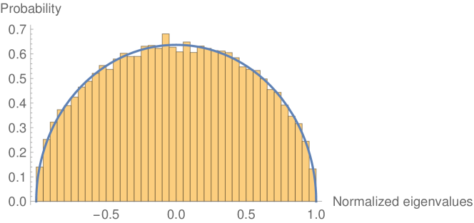
Figure 1: The distribution of normalized eigenvalues for the matrix $-K_{ij}/(2\sqrt{N})$.

The lowest eigenvalue, $\lambda_{1}=-0.0707$ is roughly minus the square root of the sparseness index. By using the decomposition (2), the Hamiltonian is written as a sum of oscillators:

$$H=\sum_{n}(\lambda_{n}+D)x_{n}^{2},$$ (3)

where

$$x_{n}=\sum_{i}S_{i}u_{ni},$$ (4)

is the projection of the lattice spin configuration over the eigenvector $u_{n}$. In our model, with equilibrated ferro- and anti-ferro couplings, the $u_{n}$ vectors corresponding to the lowest $\lambda_{n}$ have large ${\rm Tr}|u_{n}|$, but relatively small ${\rm Tr}(u_{n})$. That is, the typical configurations have large $\langle S^{2}\rangle$, but small magnetizations $\langle S\rangle$. This may change if the proportion of ferro- to anti-ferro bonds changes.

The variables $x_{n}$ are constrained to take discrete values in the interval:

$$-{\rm Tr}|u_{n}|\leq x_{n}\leq{\rm Tr}|u_{n}|.$$ (5)

In the model, the average value of ${\rm Tr}|u_{n}|$ is $0.8\sqrt{N}$, that is around 196. In addition, the $x_{n}$ variables are not independent. Indeed, for a given spin configuration, we may write:

$$\vec{S}=\sum_{n}(\vec{S}\cdot u_{n})u_{n}=\sum_{n}x_{n}u_{n},$$ (6)

and then, using orthogonality of the $u_{n}$:

$$\vec{S}\cdot\vec{S}=\sum_{n}x_{n}^{2}.$$ (7)

The l.h.s. of Eq. (7) takes values between 0 and $N$.

The partition function in our model can thus be written:

$$Z=\left(\prod_{n}Z_{n}\right)\Theta\left(N-\sum_{n}x_{n}^{2}\right),$$ (8)

where

$$Z_{n}=\sum_{x_{n}}e^{-(\lambda_{n}+D)x_{n}^{2}/T},$$ (9)

and $\Theta$ is the step (Heavyside) function: $\Theta(y)=1$ when $y>0$, and $\Theta(y)=0$ for $y<0$.

3 The continuous approximation to $Z_{n}$

As mentioned, the $x_{n}$ take discrete values in the interval given by Eq. (5). There is a single configuration for which $x_{n}={\rm Tr}|u_{n}|$. In that case $S_{i}={\rm Sign}(u_{ni})$. But there are plenty of configurations with $x_{n}\approx 0$. In the large $N$ limit, the projections of spin configurations are quasi-continuous and distributed according to the density:

$$\rho(x_{n})=\sqrt{\frac{3}{4\pi}}e^{-3x_{n}^{2}/4}.$$ (10)

In other words, the projection of $\vec{S}$ over $u_{n}$ behaves as a single $S=1$ spin.

The mode partition function $Z_{n}$ can be written:

$$Z_{n}\approx\int_{-{\rm Tr}|u_{n}|}^{{\rm Tr}|u_{n}|}e^{-\omega_{n}x_{n}^{2}}~{}{\rm d}x_{n},$$ (11)

where the frequencies $\omega_{n}$ are given by:

$$\omega_{n}=\frac{\lambda_{n}+D}{T}+\frac{3}{4}.$$ (12)

This quasi-continuous approximation is essential for the results of the paper. It can be seen to be equivalent to a mean field approximation.

4 The phase transition

The effective frequencies given in Eq. (12) have two contributions. The first coming from the system parameters, and a second “entropic” contribution coming from the number of available states. Even if $(\lambda_{n}+D)<0$ it should overcome the second contribution in order to $\omega_{n}$ to become negative.

And, indeed, there is a change of behavior when $\omega_{n}$ changes sign. In particular $\omega_{1}$, corresponding to the lowest eigenvalue $\lambda_{1}$. For $D>|\lambda_{1}|$, $\omega_{1}$ is always greater than zero. When $0\leq D<|\lambda_{1}|$, one can define a critical temperature $T_{c}=4(|\lambda_{1}|-D)/3$ signaling the transition from the paramagnetic state (PM) to the spin glass (SG). The phase diagram of the studied BCM is shown in Fig. 2.

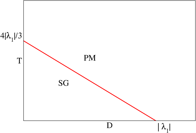
Figure 2: Phase diagram of the studied BCM.

It may be verified, in Ising or other systems in low dimensions, that the critical temperature deduced from the change of sign in $\omega_{1}$ is related to a mean field approximation. In our model, with relatively high coordination numbers, this approximation should be nearly exact.

5 Small oscillations

The regime of small oscillations is characterized by $\sum_{n}x_{n}^{2}<<N$. In the model, this regime can be reached with relatively high values of $D$ or $T$. The $\Theta$ function in this case evaluates to 1, and the mode partition functions, $Z_{n}$ can be independently computed.

5.1 The mean value $\langle x_{n}^{2}\rangle$

In the calculation of $\langle x_{n}^{2}\rangle$ we shall distinguish the cases $\omega_{n}>0$ and $\omega_{n}<0$.

$$\omega_{n}>0:~{}~{}~{}\langle x_{n}^{2}\rangle=\frac{1}{2\omega_{n}}\left(1-\frac{\sqrt{\omega_{n}}~{}{\rm Tr}|u_{n}|~{}e^{-\omega_{n}({\rm Tr}|u_{n}|)^{2}}}{\sqrt{\pi}~{}{\rm Erf}(\sqrt{\omega_{n}}~{}{\rm Tr}|u_{n}|)/2}\right),$$ (13)

where ${\rm Erf}(y)=2\int_{0}^{y}\exp(-t^{2}){\rm d}t/\sqrt{\pi}$ is the error function. The limiting values are:

$$\langle x_{n}^{2}\rangle=0,~{}~{}T\to 0~{}~{}{\rm and}~{}~{}D>|\lambda_{n}|,$$ (14)

$$\langle x_{n}^{2}\rangle=2/3,~{}~{}T\to\infty,$$ (15)

$$\langle x_{n}^{2}\rangle=({\rm Tr}|u_{n}|)^{2}/3,~{}~{}\omega_{n}\to 0.$$ (16)

On the other hand,

$$\omega_{n}<0:~{}~{}~{}\langle x_{n}^{2}\rangle=\frac{1}{2|\omega_{n}|}\left(-1+\frac{\sqrt{|\omega_{n}|}~{}{\rm Tr}|u_{n}|}{{\rm DawsonF}(\sqrt{|\omega_{n}|}~{}{\rm Tr}|u_{n}|)}\right),$$ (17)

where ${\rm DawsonF}(y)=e^{-y^{2}}\int_{0}^{y}e^{t^{2}}{\rm d}t$ is the Dawson function. The limiting values are:

$$\langle x_{n}^{2}\rangle=({\rm Tr}|u_{n}|)^{2},~{}~{}T\to 0,$$ (18)

$$\langle x_{n}^{2}\rangle=({\rm Tr}|u_{n}|)^{2}/3,~{}~{}\omega_{n}\to 0.$$ (19)

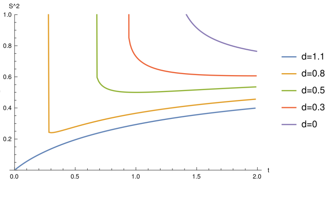
Figure 3: $\langle S^{2}\rangle$ as a function of $t=T/|\lambda_{1}|$ and $d=D/|\lambda_{1}|$ in the BCM.

5.2 The mean value of $S^{2}$

The mean value of $S^{2}$ is defined as:

$$\langle S^{2}\rangle=\frac{1}{N}\left\langle\sum_{n}x_{n}^{2}\right\rangle.$$ (20)

In the small oscillations regime, the mode averages can be independently computed. The results are shown in Fig. 3.

All of the curves tend to 2/3 in the high-$T$ limit and exhibit an abrupt rise as $t$ approaches $t_{c}$. The transition for $d\lesssim 0.7$ is beyond the plot range and beyond the validity range of the small oscillations approximation because, according to Eq. (16), near the transition point the lowest modes make contributions $({\rm Tr}|u_{n}|)^{2}/3\approx 0.2~{}N$ to $\langle S^{2}\rangle$.

Note that, for high enough values of $d$, there are points inside the PM phase at which ${\rm d}\langle S^{2}\rangle/{\rm d}T=0$. They are related to the mentioned rise of $\langle S^{2}\rangle$ as $T$ approaches $T_{c}$.

5.3 The mean energy

The mean energy per spin is defined as:

$$\langle E\rangle=\frac{1}{N}\left\langle\sum_{n}\lambda_{n}x_{n}^{2}\right\rangle.$$ (21)

In the small oscillations regime it can be straightforwardly computed from the previous results. For temperatures greater than $T_{c}$, all the $\omega_{n}$ are greater than zero and:

$$\langle E\rangle\approx\frac{1}{N}\sum_{n}\frac{2}{3}\lambda_{n}\to 0,~{}~{}T\to\infty.$$ (22)

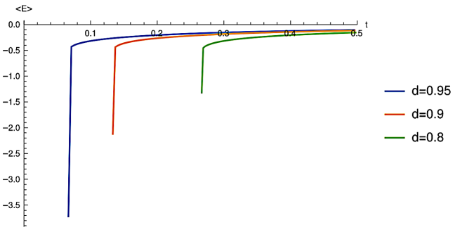
Figure 4: $\langle E\rangle$ as a function of the reduced $t$ and $d$ in the BCM. Each curve starts at the corresponding $t_{c}$ and ends at $t=0.5$.

The results are shown in Fig. 4 for $d>0.8$ and $t\geq t_{c}$, the range in which the small oscillations approximation holds. Notice the very high slope at $t_{c}$.

6 Discussion

In the paper, the interaction matrix of a spin system is diagonalized in order to represent the system as a set of constrained oscillators. For large enough lattices, a quasi-continuous approximation to the projections of the spin configurations over the eigenvectors allows the exact computation of oscillator frequencies, leading to a new mean field theory for the spin system. In quality of illustration, the method is applied to obtain observables in a disordered, frustrated BCM with 60,000 spins.

In the small oscillations regime, the oscillators are decoupled. This approximation holds at large enough temperatures or high values of the $D$ parameter. Below the transition temperature, the constrained sum, Eq. (8), shall be used. We stress that this expression is very well suited for Monte Carlo evaluations. In this way, a mean field Monte Carlo scheme may emerge. Work along this direction is in progress.

Acknowledgements Authors acknowledge the Cuban Agency for Nuclear Energy and Advanced Technologies (AENTA) and the the Office of External Activities of the Abdus Salam Centre for Theoretical Physics (ICTP) for support. The authors are grateful to C. Chatelain for suggestions and criticism.

References

- [1] K. Binder, A.P. Young. Spin glasses: Experimental facts, theoretical concepts, and open questions. Reviews of Modern Physics, Vol. 58, (1986) 801.
- [2] J.A. Mydosh. Spin glasses: redux: an updated experimental/materials survey. Rep. Prog. Phys. 78 (2015) 052501.
- [3] M. Mezard, G. Parisi, M.A. Virasoro. Spin glass theory and beyond. Lecture Notes in Physics Vol. 9. World Scientific. Singapore 1987.
- [4] Robert H. Swendsen and Jian-Sheng Wang. Replica Monte Carlo Simulation of Spin-Glasses. Phys. Rev. Lett. 57 (1986) 2607.
- [5] Koji Hukushima and Koji Nemoto. Exchange Monte Carlo method and application to spin glass simulation. Journal of the Phys. Soc. of Japan 65 (1996) 1604-1608.
- [6] Helmut G. Katzgraber, Matteo Palassini and A. P. Young (2001). Monte Carlo Simulations of Spin Glasses at Low Temperatures. Phys. Rev. B 63, 184422.
- [7] Tommaso Castellani and Andrea Cavagna.Spin-Glass Theory for Pedestrians. J. Stat. Mech. (2005) P05012. DOI 10.1088/1742-5468/2005/05/P05012.
- [8] Francesco Zamponi (2014). Mean field theory of spin glasses. arXiv:1008.4844.
- [9] Leticia F. Cugliandolo. Course 7: Dynamics of Glassy Systems. In: Barrat, JL., Feigelman, M., Kurchan, J., Dalibard, J. (eds) Slow Relaxations and nonequilibrium dynamics in condensed matter. Les Houches-École d’Été de Physique Theorique, vol 77. Springer, Berlin, Heidelberg. https://doi.org/10.1007/978-3-540-44835-8_7.
- [10] J.A. Plascak, J.G. Moreira and F.C. Barreto. Mean field solution of the general spin Blume-Capel model. Physics Letters A 173 (1993) 360-364.
- [11] D. Peña Lara, J. E. Diosa, and C. A. Lozano. Blume-Capel spin-glass model for Fe-Mn-Al alloys. Phys. Rev. E 87, 032108 (2013).
- [12] L. Leuzzi, M. Paoluzzi, and A. Crisanti. Random Blume-Capel model on a cubic lattice: First-order inverse freezing in a three-dimensional spin-glass system. Phys. Rev. B 83, 014107 (2011).
- [13] Florent Benaych-Georges and Antti Knowles. Lectures on the local semicircle law for Wigner matrices. In Advanced topics in random matrices, 1–90, Panor. Synthèses, 53, Soc. Math. France, Paris, 2017.
- [14] Laszlo Erdos, Benjamin Schlein and Horng-Tzer Yau. Local semicircle law and complete delocalization for Wigner random matrices. Commun. Math. Phys. 287, pages 641–655 (2009).