Randomized algorithms for computing the generalized tensor SVD based on the tubal product

Abstract

This work deals with developing two fast randomized algorithms for computing the generalized tensor singular value decomposition (GTSVD) based on the tubal product (t-product). The random projection method is utilized to compute the important actions of the underlying data tensors and use them to get small sketches of the original data tensors, which are easier to be handled. Due to the small size of the sketch tensors, deterministic approaches are applied to them to compute their GTSVDs. Then, from the GTSVD of the small sketch tensors, the GTSVD of the original large-scale data tensors is recovered. Some experiments are conducted to show the effectiveness of the proposed approach.

[label1]organization=Center for Artificial Intelligence Technology, Skolkovo Institute of Science and Technology, Moscow, Russia,  s.asl@skoltech.ru, [label2]organization=Department of Mathematics, Colorado State University, Fort Collins, USA,  Ugochukwu.Ugwu@colostate.edu,

1 Introduction

The Singular Value Decomposition (SVD) is a matrix factorization that has been widely used in many applications, such as signal processing and machine learning [1]. It can compute the best low-rank approximation of a matrix in the least-squares sense for any invariant matrix norm. When applied to a single matrix, the SVD can effectively capture orthonormal bases associated with the four fundamental subspaces. The idea of extending SVD to a pair of matrices was first proposed in [2, 3], and is referred to as the generalized SVD (GSVD). The GSVD has found practical applications in solving inverse problems [4], as well as in genetics [5, 6].

However, the classical SVD or GSVD is prohibitive for computing low-rank approximations of large-scale data matrices. To circumvent this difficulty, randomization is often employed to efficiently compute the SVD or GSVD of such matrices, see, e.g., [7, 8, 9]. Randomized SVD and GSVD methods first capture the range of the given data matrices through multiplication with random matrices or by simply sampling some columns of the original data matrices. Then, generate an orthonormal basis to determine small matrix sketches that are easy to handle. The desired SVD or GSVD of the original data is recovered from the SVD or GSVD of the small sketches.

The benefits of randomized algorithms make them ubiquitous tools in numerical linear algebra. Specifically, randomized approaches provide stable approximations and can be implemented in parallel to significantly speed up SVD or GSVD computation of large-scale matrices. Extensions of randomized SVD to third-order tensors using different tensor decompositions have been considered in the literature, see, e.g., [10, 11, 12, 13, 14, 15], and references therein.

Here, we will focus on the use of tensor SVD (T-SVD) approach proposed in [16, 17]. The T-SVD approach uses the tensor t-product first introduced in [17] to multiply two or more tensors. The t-product between two third-order tensors, which will be defined below, is computed by first transforming the given tensors into the Fourier domain along the third dimension, evaluating matrix-matrix products in the Fourier domain, and then computing the inverse Fourier transform of the result. The T-SVD has similar properties as the classical SVD because its truncation version provides the best tubal rank approximation in the least-squares sense. This is in contrast to the Tucker decomposition [18, 19] or the canonical polyadic decomposition [20, 21].

The GSVD has been generalized to third-order tensors based on the T-SVD approach in [22, 23], and applied to image processing. We will refer to this generalization as the Generalized Tensor SVD (GTSVD). Motivated by [8, 9], we develop two fast randomized algorithms for computing the GTSVD. The key contributions of this work are as follows:

• We develop two fast randomized algorithms for the computation of the GTSVD based on the t-product [16, 17]. The proposed algorithms achieve several orders of magnitude acceleration compared to the existing algorithms. This makes it of more practical interest for big-data processing and real-time applications.

• We provide convincing computer simulations to demonstrate the applicability of the proposed randomized algorithm. In particular, we provide a simulation for the image restoration application.

The structure of this paper is as follows. Section 2 provides preliminaries associated with third-order tensors and the t-product [16, 17]. Here, we introduce the T-SVD model and the necessary algorithms for its computations. In Section 3, we present the GSVD, and its extension to third-order tensors, i.e., the GTSVD framework. Two randomized GTSVD algorithms are proposed in Section 4 with their error analyses shown in Section 5. Computer-simulated results are reported in Section 6. Section 7 presents concluding remarks.

2 Basic definitions and concepts

We adopt the same notations used in [24] in this paper. So, to represent a tensor, a matrix, and a vector we use an underlined bold capital letter, a bold capital letter, and a bold lower letter. Slices are important subtensors that are generated by fixing all but two modes. In particular, for a third-order tensor $\underline{{\bf X}},$ the three types slices $\underline{{\bf X}}(:,:,k),\,\underline{{\bf X}}(:,j,:),\,\underline{{\bf X}}(i,:,:)$ are called frontal, lateral and horizontal slices. For convenience, sometimes in the paper, we use the equivalent notation $\underline{{\bf X}}_{i}\equiv\underline{{\bf X}}(;,:,i)$. Fibers are generated by fixing all but one mode, so they are vectors. For a third-order tensor $\underline{{\bf X}},$ the fiber $\underline{{\bf X}}(i,j,:)$ is called a tube. The notation “conj” denotes the component-wise complex conjugate of a matrix. The Frobenius norm of matrices or tensors is denoted by $\|.\|$ and $\|.\|_{\infty}$ stands for the norm infinity of tensors. The notation $\|.\|_{2}$ stands for the Euclidean norm of vectors and the spectral norm of matrices. For a positive definite matrix ${\bf S}$, the weighted inner product norm is defined as $\|{\bf X}\|_{\bf S}=\sqrt{{\rm Tr}({\bf X}^{T}{\bf S}{\bf X})}$ where “${\rm Tr}$” is the trace operator. The mathematical expectation is represented by $\mathbb{E}$. The singular values of a matrix ${\bf X}$, are denoted by $\sigma_{1},\,\sigma_{2},\ldots,\sigma_{R}$ where $R$ is the rank of the matrix ${\bf X}$. We now present the next definitions, which we need in our presentation.

Definition 1.

(t-product) Let $\underline{\mathbf{X}}\in\mathbb{R}^{I_{1}\times I_{2}\times I_{3}}$ and $\underline{\mathbf{Y}}\in\mathbb{R}^{I_{2}\times I_{4}\times I_{3}}$, the tubal product (t-product) $\underline{\mathbf{X}}*\underline{\mathbf{Y}}\in\mathbb{R}^{I_{1}\times I_{4}\times I_{3}}$ is defined as follows

$$\underline{\mathbf{C}}=\underline{\mathbf{X}}*\underline{\mathbf{Y}}={\rm fold}\left({{\rm circ}\left(\underline{\mathbf{X}}\right){\rm unfold}\left(\underline{\mathbf{Y}}\right)}\right),$$ (1)

where

$${\rm circ}\left(\underline{\mathbf{X}}\right)=\begin{bmatrix}\underline{\mathbf{X}}(:,:,1)&\underline{\mathbf{X}}(:,:,I_{3})&\cdots&\underline{\mathbf{X}}(:,:,2)\\ \underline{\mathbf{X}}(:,:,2)&\underline{\mathbf{X}}(:,:,1)&\cdots&\underline{\mathbf{X}}(:,:,3)\\ \vdots&\vdots&\ddots&\vdots\\ \underline{\mathbf{X}}(:,:,I_{3})&\underline{\mathbf{X}}(:,:,I_{3}-1)&\cdots&\underline{\mathbf{X}}(:,:,1)\end{bmatrix},$$

and

$${\rm unfold}(\underline{\mathbf{Y}})=\begin{bmatrix}\underline{\mathbf{Y}}(:,:,1)\\ \underline{\mathbf{Y}}(:,:,2)\\ \vdots\\ \underline{\mathbf{Y}}(:,:,I_{3})\end{bmatrix},\hskip 14.22636pt\underline{\mathbf{Y}}={\rm fold}\left({\rm unfold}\left(\underline{\mathbf{Y}}\right)\right).$$

Definition 2.

(Transpose) The transpose of a tensor $\underline{\mathbf{X}}\in\mathbb{R}^{I_{1}\times I_{2}\times I_{3}}$ is denoted by $\underline{\mathbf{X}}^{T}\in\mathbb{R}^{I_{2}\times I_{1}\times I_{3}}$ obtained by applying the transpose to all frontal slices of the tensor $\underline{\mathbf{X}}$ and reversing the order of the transposed frontal slices 2 through $I_{3}$.

Definition 3.

(Identity tensor) The identity tensor $\underline{\mathbf{I}}\in\mathbb{R}^{I_{1}\times I_{1}\times I_{3}}$ is a tensor whose first frontal slice is an identity matrix of size $I_{1}\times I_{1}$ and all other frontal slices are zero. It is easy to show $\underline{{\bf I}}*\underline{{\bf X}}=\underline{{\bf X}}$ and $\underline{{\bf X}}*\underline{{\bf I}}=\underline{{\bf X}}$ for all tensors of conforming sizes.

Definition 4.

(Orthogonal tensor) We all that a tensor $\underline{\mathbf{X}}\in\mathbb{R}^{I_{1}\times I_{1}\times I_{3}}$ is orthogonal if ${\underline{\mathbf{X}}^{T}}*\underline{\mathbf{X}}=\underline{\mathbf{X}}*{\underline{\mathbf{X}}^{T}}=\underline{\mathbf{I}}$.

Definition 5.

(f-diagonal tensor) If all frontal slices of a tensor are diagonal then the tensor is called an f-diagonal tensor.

Definition 6.

(Moore-Penrose pseudoinverse of a tensor) Let $\underline{\bf X}\in\mathbb{R}^{I_{1}\times I_{2}\times I_{3}}$ be given. The Moore-Penrose (MP) pseudoinverse of the tensor $\underline{\bf X}$ is denoted by $\underline{\bf X}^{{\dagger}}\in\mathbb{R}^{I_{2}\times I_{1}\times I_{3}}$ and is a unique tensor satisfying the following four equations:

$$\underline{\bf X}^{{\dagger}}*\underline{\bf X}*\underline{\bf X}^{{\dagger}}=\underline{\bf X}^{{\dagger}},\quad\underline{\bf X}*\underline{\bf X}^{{\dagger}}*\underline{\bf X}=\underline{\bf X},$$

$$(\underline{\bf X}*\underline{\bf X}^{{\dagger}})^{T}=\underline{\bf X}*\underline{\bf X}^{{\dagger}},\quad(\underline{\bf X}^{{\dagger}}*\underline{\bf X})^{T}=\underline{\bf X}^{{\dagger}}*\underline{\bf X}.$$

The MP pseudoinverse of a tensor can also be computed in the Fourier domain as shown in Algorithm 2.

The inverse of a tensor is a special case of the MP pseudoinverse of tensors. The inverse of $\underline{\bf X}\in\mathbb{R}^{I_{1}\times I_{1}\times I_{3}}$ is denoted by $\underline{\bf X}^{-1}\in\mathbb{R}^{I_{1}\times I_{1}\times I_{3}}$ is a unique tensor satisfying $\underline{\bf X}*\underline{\bf X}^{-1}=\underline{\bf X}^{-1}*\underline{\bf X}=\underline{\bf I},$ where $\underline{\bf I}\in\mathbb{R}^{I_{1}\times I_{1}\times I_{3}}$ is the identity tensor The inverse of a tensor can be also computed in the Fourier domain by replacing the MATLAB command “inv” in Line 3 of Algorithm 2.

Input : Two data tensors $\underline{\mathbf{X}}\in{\mathbb{R}^{{I_{1}}\times{I_{2}}\times{I_{3}}}},\,\,\underline{\mathbf{Y}}\in{\mathbb{R}^{{I_{2}}\times{I_{4}}\times{I_{3}}}}$

Output : t-product $\underline{\mathbf{C}}=\underline{\mathbf{X}}*\underline{\mathbf{Y}}\in\mathbb{R}^{I_{1}\times I_{4}\times I_{3}}$

1 $\widehat{\underline{\mathbf{X}}}={\rm fft}\left({\underline{\mathbf{X}},[],3}\right)$;

2 $\widehat{\underline{\mathbf{X}}}={\rm fft}\left({\underline{\mathbf{Y}},[],3}\right)$;

3 for $i=1,2,\ldots,\lceil\frac{I_{3}+1}{2}\rceil$ do

4       $\widehat{\underline{\mathbf{C}}}\left({:,:,i}\right)=\widehat{\underline{\mathbf{X}}}\left({:,:,i}\right)\,\widehat{\underline{\mathbf{Y}}}\left({:,:,i}\right)$;

5      

6 end for

7for $i=\lceil\frac{I_{3}+1}{2}\rceil+1\ldots,I_{3}$ do

8       $\widehat{\underline{\mathbf{C}}}\left({:,:,i}\right)={\rm conj}(\widehat{\underline{\mathbf{C}}}\left({:,:,I_{3}-i+2}\right))$;

9 end for

$\underline{\mathbf{C}}={\rm ifft}\left({\widehat{\underline{\mathbf{C}}},[],3}\right)$;

Algorithm 1 The t-product of two tensors [17, 25]

Input : The data tensor $\underline{\mathbf{X}}\in{\mathbb{R}^{{I_{1}}\times{I_{2}}\times{I_{3}}}}$

Output : Moore-Penrose pseudoinvers $\underline{\mathbf{X}}^{{\dagger}}\in\mathbb{R}^{I_{2}\times I_{1}\times I_{3}}$

1 $\widehat{\underline{\mathbf{X}}}={\rm fft}\left({\underline{\mathbf{X}},[],3}\right)$;

2 for $i=1,2,\ldots,\lceil\frac{I_{3}+1}{2}\rceil$ do

3       $\widehat{\underline{\mathbf{C}}}\left({:,:,i}\right)={\rm pinv}\,(\widehat{{\bf X}}(:,:,i))$;

4      

5 end for

6for $i=\lceil\frac{I_{3}+1}{2}\rceil+1,\ldots,I_{3}$ do

7       $\widehat{\underline{\mathbf{C}}}\left({:,:,i}\right)={\rm conj}(\widehat{\underline{\mathbf{C}}}\left({:,:,I_{3}-i+2}\right))$;

8 end for

$\underline{\mathbf{X}}^{{\dagger}}={\rm ifft}\left({\widehat{\underline{\mathbf{C}}},[],3}\right)$;

Algorithm 2 Fast Moore-Penrose pseudoinvers computation of the tensor $\underline{\bf X}$

It can be proven that for a tensor ${\bf X}\in\mathbb{R}^{I_{1}\times I_{2}\times I_{3}}$, we have

$$\|\underline{{\bf X}}\|^{2}_{F}=\frac{1}{I_{3}}\sum_{i=1}^{I_{3}}\|\widehat{\underline{{\bf X}}}(:,:,i)\|_{F}^{2},$$ (2)

where $\widehat{\underline{{\bf X}}}(:,:,i)$ is the $i$-th frontal slice of the tensor $\widehat{\underline{{\bf X}}}={\rm fft}(\underline{{\bf X}},[],3)$, see [25, 14].

2.1 Tensor SVD (T-SVD), Tensor QR (T-QR) decomposition and Tensor LU (T-LU) decomposition

The classical matrix decompositions such as QR, LU, and SVD can be straightforwardly generalized to tenors based on the t-product. Given a tensor $\underline{{\bf X}}\in\mathbb{R}^{I_{1}\times I_{2}\times I_{3}},$ the tensor QR (T-QR) decomposition represents the tensor $\underline{\bf X}$ as $\underline{{\bf X}}=\underline{{\bf Q}}*\underline{{\bf R}}$ and can be computed through Algorithm 3. By a slight modification of Algorithm 3, the tensor LU (T-LU) decomposition and the tensor SVD (T-SVD) can be computed. More precisely, in line 4 of Algorithm 3, we replace the LU decomposition and the SVD of frontal slices $\widehat{\underline{{\bf X}}}(:,:,i),\,i=1,2,\ldots,I_{3},$ instead of the QR decomposition.

The tensor SVD (T-SVD) expresses a tensor as the t-product of three tensors. The first and last tensors are orthogonal while the middle tensor if an f-diagonal tensor. Let $\underline{{\bf X}}\in\mathbb{R}^{I_{1}\times I_{2}\times I_{3}}$, then the T-SVD gives the following model:

$$\underline{{\bf X}}\approx\underline{\bf U}*\underline{\bf S}*\underline{\bf V}^{T},$$

where $\underline{\bf U}\in\mathbb{R}^{I_{1}\times R\times I_{3}},\,\underline{\bf S}\in\mathbb{R}^{R\times R\times I_{3}},$ and $\underline{\bf V}\in\mathbb{R}^{I_{2}\times R\times I_{3}}$. The tensors $\underline{\bf U}$ and $\underline{\bf V}$ are orthogonal, while the tensor $\underline{\bf S}$ is f-diagonal. The generalization of the T-SVD to tensors of order higher than three is done in [26]. The T-SVD can be computed via Algorithm 4.

Input : The data tensor $\underline{\mathbf{X}}\in{\mathbb{R}^{{I_{1}}\times{I_{2}}\times{I_{3}}}}$

Output : The T-QR decomposition of the tensor $\underline{\bf X}=\underline{\bf Q}*\underline{\bf R}$

1 $\widehat{\underline{\mathbf{X}}}={\rm fft}\left({\underline{\mathbf{X}},[],3}\right)$;

2 for $i=1,2,\ldots,\lceil\frac{I_{3}+1}{2}\rceil$ do

3       $[\widehat{\underline{\mathbf{Q}}}\left({:,:,i}\right),\underline{\widehat{{\bf R}}}(:,:,i)]={\rm qr}\,(\underline{\widehat{{\bf X}}}(:,:,i),0)$;

4      

5 end for

6for $i=\lceil\frac{I_{3}+1}{2}\rceil+1\ldots,I_{3}$ do

7       $\widehat{\underline{\mathbf{Q}}}\left({:,:,i}\right)={\rm conj}(\widehat{\underline{\mathbf{Q}}}\left({:,:,I_{3}-i+2}\right))$;

8       $\widehat{\underline{\mathbf{R}}}\left({:,:,i}\right)={\rm conj}(\widehat{\underline{\mathbf{R}}}\left({:,:,I_{3}-i+2}\right))$;

9 end for

10$\underline{\mathbf{Q}}={\rm ifft}\left({\widehat{\underline{\mathbf{Q}}},[],3}\right)$;

$\underline{\mathbf{R}}={\rm ifft}\left({\widehat{\underline{\mathbf{R}}},[],3}\right)$;

Algorithm 3 The T-QR decomposition of the tensor $\underline{\bf X}$

Input : The data tensor $\underline{\mathbf{X}}\in{\mathbb{R}^{{I_{1}}\times{I_{2}}\times{I_{3}}}}$ and a target tubal rank $R$

Output : The truncated T-SVD of the tensor $\underline{\bf X}\approx\underline{\bf U}*\underline{\bf S}*\underline{\bf V}^{T}$

1 $\widehat{\underline{\mathbf{X}}}={\rm fft}\left({\underline{\mathbf{X}},[],3}\right)$;

2 for $i=1,2,\ldots,\lceil\frac{I_{3}+1}{2}\rceil$ do

3       $[\widehat{\underline{\mathbf{U}}}\left({:,:,i}\right),\widehat{\underline{\bf S}}(:,:,i),\widehat{\underline{{\bf V}}}(:,:,i)]={\rm svds}\,(\widehat{\underline{{\bf X}}}(:,:,i),R)$;

4      

5 end for

6for $i=\lceil\frac{I_{3}+1}{2}\rceil+1,\ldots,I_{3}$ do

7       $\widehat{\underline{\mathbf{U}}}\left({:,:,i}\right)={\rm conj}(\widehat{\underline{\mathbf{U}}}\left({:,:,I_{3}-i+2}\right))$;

8       $\widehat{\underline{\mathbf{S}}}\left({:,:,i}\right)=\widehat{\underline{\mathbf{S}}}\left({:,:,I_{3}-i+2}\right)$;

9       $\widehat{\underline{\mathbf{V}}}\left({:,:,i}\right)={\rm conj}(\widehat{\underline{\mathbf{V}}}\left({:,:,I_{3}-i+2}\right))$;

10 end for

$\underline{\mathbf{U}}={\rm ifft}\left({\widehat{\underline{\mathbf{U}}},[],3}\right)$; $\underline{\mathbf{S}}={\rm ifft}\left({\widehat{\underline{\mathbf{S}}},[],3}\right)$; $\underline{\mathbf{V}}={\rm ifft}\left({\widehat{\underline{\mathbf{V}}},[],3}\right)$

Algorithm 4 The truncated T-SVD decomposition of the tensor $\underline{\bf X}$

3 Generalized singular value decomposition (GSVD) and its extension to tensors based on the t-product (GTSVD)

In this section, the GSVD and its extension to tensors based on the t-product are introduced. The GSVD is a generalized version of the classical SVD, which is applied to a pair of matrices. The SVD was generalized in [2] from two different perspectives. More precisely, from the SVD, it is known that each matrix ${\bf X}\in\mathbb{R}^{I_{1}\times I_{2}}$ can be decomposed in the form ${\bf X}={\bf U}{\bf S}{\bf V}^{T}$ where ${\bf U}\in\mathbb{R}^{I_{1}\times I_{1}}$ and ${\bf V}\in\mathbb{R}^{I_{2}\times I_{2}}$ are orthogonal matrices and the ${\bf S}={\rm diag}(\sigma_{1},\sigma_{2},\ldots,\sigma_{\min\{I_{1},I_{2}\}})\in\mathbb{R}^{I_{1}\times I_{2}}$ is a diagonal matrix with singular values $\sigma_{1}\geq\sigma_{2}\geq\ldots\geq\sigma_{R}>\sigma_{R+1}=\ldots=\sigma_{\min\{I_{1},I_{2}\}}=0$ and ${\rm rank}({\bf X})=R.$ Denoting the set of singular values of the matrix ${\bf X}$ as $\sigma({\bf X})=\{\sigma_{1},\sigma_{2},\ldots,\sigma_{\min\{I_{1},I_{2}\}}\}$, it is known that

$$\sigma_{i}\in\sigma({\bf X})\longrightarrow{\rm det}({\bf X}^{T}{\bf X}-\sigma_{i}^{2}{\bf I})=0,$$ (3)

$$\sigma_{i}\in\sigma({\bf X})\longrightarrow\sigma_{i}\textrm{\,is a stationary point of\,}\frac{\|{\bf X}{\bf z}\|_{2}}{\|{\bf z}\|_{2}}.$$ (4)

Based on (3) and 4, the SVD was generalized in the following straightforward ways:

$$\textrm{Find\,}\sigma\geq 0\,\textrm{such that\,\,}{\rm det}({\bf X}^{T}{\bf X}-\sigma^{2}{\bf Y}^{T}{\bf Y})=0,$$ (5)

$$\textrm{Find the stationary values of\,}\frac{\|{\bf X}{\bf z}\|_{\bf S}}{\|{\bf z}\|_{\bf T}},$$ (6)

where ${\bf Y}\in\mathbb{R}^{I_{3}\times I_{2}}$ is an arbitrary matrix and ${\bf S}\in\mathbb{R}^{I_{2}\times I_{2}}$ and ${\bf T}\in\mathbb{R}^{I_{1}\times I_{1}}$ are positive definitive matrices. In this paper, we only consider the generalization of form (5) and its extension to tensors based on the t-product, see see [2] for details about GSVD with formulation (6). To this end, let us denote the set of all points satisfying (5) as $\sigma({\bf X},{\bf Y})=\{\sigma|\sigma\geq 0,\,{\rm det}({\bf X}^{T}{\bf X}-\sigma^{2}{\bf Y}^{T}{\bf Y})=0\},$ which are called ${\bf Y}$-singular values of the matrix ${\bf X}$. It was shown in [2] that given ${\bf X}\in\mathbb{R}^{I_{1}\times I_{2}},\,\,I_{1}\geq I_{2}$ and ${\bf Y}\in\mathbb{R}^{I_{3}\times I_{2}},\,I_{3}\geq I_{2}$ there exist orthogonal matrices ${\bf U}\in\mathbb{R}^{I_{1}\times I_{1}},\,{\bf V}\in\mathbb{R}^{I_{3}\times I_{3}}$ and a nonsingular matrix ${\bf Z}\in\mathbb{R}^{I_{2}\times I_{2}}$ such that

$${\bf U}^{T}{\bf X}{\bf Z} = {\rm diag}(\alpha_{1},\cdots,\alpha_{I_{2}}),\quad\alpha_{i}\in[0,1]$$ (7)

$${\bf V}^{T}{\bf Y}{\bf Z} = {\rm diag}(\beta_{1},\cdots,\beta_{I_{2}}),\quad\beta_{i}\in[0,1]$$ (8)

where $\alpha_{i}^{2}+\beta_{i}^{2}=1$ with the ratios $\beta_{i}/\alpha_{i}$ of nondecreasing order for $i=1,2,\ldots,I_{2}$. A more general SVD was proposed in [3] where a more computationally stable algorithm was also developed to compute it. In the following, the latter GSVD is introduced, which will be considered in our paper.

Theorem 1.

[3] Let two matrices ${\bf X}\in\mathbb{R}^{I_{1}\times I_{2}}$ and ${\bf Y}\in\mathbb{R}^{I_{3}\times I_{2}}$ be given and assume that the SVD of the matrix ${\bf C}=\begin{bmatrix}{\bf X}\\ {\bf Y}\end{bmatrix}$ is

$${\bf E}^{T}{\bf C}{\bf Z}=\begin{bmatrix}{\bf\Gamma}&{\bf 0}\\ {\bf 0}&{\bf 0}\end{bmatrix},$$ (9)

with the unitary matrices ${\bf E}\in\mathbb{R}^{(I_{1}+I_{3})\times(I_{1}+I_{3})},\,{\bf Z}\in\mathbb{R}^{I_{2}\times I_{2}}$ and a diagonal matrix ${\bf\Gamma}\in\mathbb{R}^{k\times k}$. Then, there exist unitary matrices ${\bf U}\in\mathbb{R}^{I_{1}\times I_{1}},\,{\bf V}\in\mathbb{R}^{I_{3}\times I_{3}}$ and ${\bf W}\in\mathbb{R}^{k\times k}$ such that

$${\bf U}^{T}{\bf X}{\bf Z}={\bf\Sigma}_{\bf X}({\bf W}^{T}{\bf\Gamma},{\bf 0}),\quad{\bf V}^{T}{\bf Y}{\bf Z}={\bf\Sigma}_{\bf Y}({\bf W}^{T}{\bf\Gamma},{\bf 0}),$$ (10)

where ${\bf\Sigma}_{\bf X}\in\mathbb{R}^{I_{1}\times k}$ and ${\bf\Sigma}_{\bf Y}\in\mathbb{R}^{I_{3}\times k}$ are defined as follows:

$${\bf\Sigma}_{X}=\begin{bmatrix}{\bf I}_{\bf X}&&\\ &{\bf S}_{\bf X}&\\ &&{\bf 0}_{\bf X}\end{bmatrix},\quad{\bf\Sigma}_{Y}=\begin{bmatrix}{\bf 0}_{\bf Y}&&\\ &{\bf S}_{\bf Y}&\\ &&{\bf I}_{\bf Y}\end{bmatrix}.$$ (11)

Here, ${\bf I}_{\bf X}\in\mathbb{R}^{c\times c}$ and ${\bf I}_{\bf Y}\in\mathbb{R}^{(k-c-d)\times(k-c-d)}$ are identity matrices, ${\bf 0}_{\bf X}\in\mathbb{R}^{(I_{1}-c-d)\times(k-c-d)}$ and ${\bf 0}_{\bf Y}\in\mathbb{R}^{(I_{3}-k+c)\times c}$ are zero matrices that may have no columns/rows and ${\bf S}_{\bf X}\in\mathbb{R}^{d\times d},\,{\bf S}_{\bf Y}\in\mathbb{R}^{d\times d}$ are diagonal matrices with diagonal elements $1>\alpha_{c+1}\geq\cdots\geq\alpha_{c+d}>0$ and $0<\beta_{c+1}\leq\cdots\leq\beta_{c+d}<1$, respectively and $\alpha_{i}^{2}+\beta_{i}^{2}=1$ for $c+1\leq i\leq c+d$. Note that $c$ and $d$ are internally defined by the matrices ${\bf X}$ and ${\bf Y}$.

It is not difficult to check that (10) is reduced to

$${\bf U}^{T}{\bf X}{\bf R}^{-1}=({\bf\Sigma}_{\bf X},{\bf 0}),\quad{\bf V}^{T}{\bf Y}{\bf R}^{-1}=({\bf\Sigma}_{\bf Y},{\bf 0}),$$ (12)

for ${\bf R}^{-1}$ defined as follows

$${\bf R}^{-1}={\bf Z}\begin{bmatrix}{\bf\Gamma}^{-1}{\bf W}&{\bf 0}\\ {\bf 0}&{\bf I}_{I_{2}-k}\end{bmatrix},$$

and if the matrix ${\bf C}$ is of full rank, then the zero blocks on the right-hand sides of (12) are removed. As we see, the first formulation (5) of the GSVD deals with two matrices ${\bf X}$ and ${\bf Y},$ and provides a decomposition of the form (12) with the same right-hand side matrix ${\bf R}^{-1}$.

The GSVD can be analogously extended to tensors based on the t-product [22, 23]. Let $\underline{\bf X},\,\underline{\bf Y}$ be two given tensors with the same number of lateral slices. Then the Generalized tensor SVD (GTSVD) decomposes the tensors $\underline{\bf X}\in\mathbb{R}^{I_{1}\times I_{2}\times I_{3}},\,\,I_{1}\geq I_{2},\,\underline{\bf Y}\in\mathbb{R}^{I_{4}\times I_{2}\times I_{3}},\,I_{4}\geq I_{2},$ jointly in the following form:

$$\underline{\bf X} = \underline{\bf U}*\underline{\bf C}*\underline{\bf Z},$$ (13)

$$\underline{\bf Y} = \underline{\bf V}*\underline{\bf S}*\underline{\bf Z},$$ (14)

where $\underline{\bf U}\in\mathbb{R}^{I_{1}\times I_{1}\times I_{3}},\,\underline{\bf V}\in\mathbb{R}^{I_{4}\times I_{4}\times I_{3}},\,\underline{\bf C}\in\mathbb{R}^{I_{1}\times I_{2}\times I_{3}},\,\underline{\bf S}\in\mathbb{R}^{I_{4}\times I_{2}\times I_{3}},\,\underline{\bf Z}\in\mathbb{R}^{I_{2}\times I_{2}\times I_{3}}$. Note that the tensors $\underline{\bf C}$ and $\underline{\bf S}$ are f-diagonal and the tensors $\underline{\bf U}$ and $\underline{\bf V}$ are orthogonal and $\underline{\bf Z}$ is nonsingular. The procedure of the computation of the GTSVD is presented in Algorithm 5. We need to apply the classical GSVD (lines 3-5) to the first $\lceil\frac{I_{3}+1}{2}\rceil$ frontal slices of the tensors $\underline{\bf X}$ and $\underline{\bf Y}$ in the Fourier domain and the rest of the slices are computed easily (Lines 6-12).

The computation of the GSVD or the GTSVD for large-scale matrices/tensors involves the computation of the SVD of some large matrices. So, it is computationally demanding and requires huge memory and resources. In recent years, the idea of randomization has been utilized to accelerate the computation of the GSVD. In [8], a randomized algorithm is proposed for the GSVD of the form (5) while [9] proposes a randomized algorithm for the GSVD of form 6. The key idea is to employ the random projection method for fast computation of the SVD, which is required in the process of computing the GSVD.

Input : The data tensors $\underline{\mathbf{X}}\in{\mathbb{R}^{{I_{1}}\times{I_{2}}\times{I_{3}}}}$ and $\underline{\mathbf{Y}}\in{\mathbb{R}^{{I_{4}}\times{I_{2}}\times{I_{3}}}}$

Output : The generalized T-SVD (GTSVD) of $\underline{\mathbf{X}}$ and $\underline{\bf Y}$ as $\underline{\mathbf{X}}=\underline{\mathbf{U}}*\underline{\mathbf{C}}*\underline{\mathbf{Z}}$ and $\underline{\mathbf{Y}}=\underline{\mathbf{V}}*\underline{\mathbf{S}}*\underline{\mathbf{Z}}$

1 $\widehat{\underline{\mathbf{X}}}={\rm fft}\left({\underline{\mathbf{X}},[],3}\right)$;

2 $\widehat{\underline{\mathbf{Y}}}={\rm fft}\left({\underline{\mathbf{Y}},[],3}\right)$;

3 for $i=1,2,\ldots,\lceil\frac{I_{3}+1}{2}\rceil$ do

4       $[\widehat{\underline{\mathbf{U}}}_{i},\,\widehat{\underline{\mathbf{V}}}_{i},\,\widehat{\underline{\mathbf{Z}}}_{i},\,\widehat{\underline{\mathbf{C}}}_{i},\,\widehat{\underline{\mathbf{S}}}_{i}]={\rm GSVD}\,(\widehat{\underline{{\bf X}}}(:,:,i),\widehat{\underline{{\bf Y}}}(:,:,i))$;

5      

6 end for

7for $i=\lceil\frac{I_{3}+1}{2}\rceil+1\ldots,I_{3}$ do

8       $\widehat{\underline{\mathbf{U}}}_{i}={\rm conj}(\widehat{\underline{\mathbf{U}}}_{I_{3}-i+2})$;

9       $\widehat{\underline{\mathbf{V}}}_{i}={\rm conj}({\underline{\mathbf{V}}}_{I_{3}-i+2})$;

10       $\widehat{\underline{\mathbf{Z}}}_{i}={\rm conj}(\widehat{\underline{\mathbf{Z}}}_{I_{3}-i+2})$;

11       $\widehat{\underline{\mathbf{C}}}_{i}=\widehat{\underline{\mathbf{C}}}_{I_{3}-i+2}$;

12       $\widehat{\underline{\mathbf{S}}}_{i}=\widehat{\underline{\mathbf{S}}}_{I_{3}-i+2}$;

13 end for

${\underline{\mathbf{U}}}={\rm ifft}\left({\widehat{\underline{\mathbf{U}}},[],3}\right)$; $\,{\underline{\mathbf{V}}}={\rm ifft}\left({\widehat{\underline{\mathbf{V}}},[],3}\right)$; $\,{\underline{\mathbf{Z}}}={\rm ifft}\left({\widehat{\underline{\mathbf{Z}}},[],3}\right)$; $\,{\underline{\mathbf{C}}}={\rm ifft}\left({\widehat{\underline{\mathbf{C}}},[],3}\right)$; $\,{\underline{\mathbf{S}}}={\rm ifft}\left({\widehat{\underline{\mathbf{S}}},[],3}\right)$;

Algorithm 5 Generalized T-SVD of $\underline{\bf X}$ and $\underline{\bf Y}$

4 Proposed fast randomized algorithms for computation of the GTSVD

In this section, we propose two randomized variants of the GTSVD Algorithm 5. The first proposed randomized algorithm is a naive modification of Algorithm 5 where we can replace the deterministic GSVD with the randomized counterpart developed in [8]. This idea is presented in Algorithm 6. Here, we can use the oversampling and the power iteration methods to improve the accuracy of the singular values of the frontal slices do not decay sufficiently fast [7].

The second proposed randomized algorithm is presented in Algorithm 7 where we first make a reduction on the given data tensors by multiplying with random tensors to capture their important actions. Then, by applying the T-QR algorithm to the mentioned compressed tensors, we can obtain orthonormal bases for them (Line 3-4 in Algorithm 7), which are used to get small sketch tensors by projecting the original data tensors onto the compressed tensors . Since the sizes of the sketch tensors are smaller than the original ones, the deterministic algorithms can be used to compute their GTSVDs. Finally, the GTSVD of the original data tensor can be recovered from the GTSVD of the compressed tensors. Note that in Algorithms 6 and 7, we need the tubal rank as input, however, this can be numerically estimated for a given approximation error bound. For example, we can use the randomized fixed-precision developed in [27] and for the case of tensors, the randomized rank-revealing algorithm proposed in [28, 29, 30] is applicable. Similar to Algorithm 6, if the frontal slices of a given tensor do not have a fast decay, the power iteration technique and the oversampling method should be used to better capture their ranges. More precisely, the random projection stages in Algorithm 7 (Lines 1-2) are replaced with the following computations

$$\underline{\bf W}_{1}=(\underline{\bf X}*\underline{\bf X}^{T})^{q}*\underline{\bf X}*\underline{\bf\Omega}_{1},$$ (15)

$$\underline{\bf W}_{2}=(\underline{\bf Y}*\underline{\bf Y}^{T})^{q}*\underline{\bf Y}*\underline{\bf\Omega}_{2}.$$ (16)

In practice, for the computations (15)-(16) to be stable, we employ the T-QR decomposition or the T-LU decomposition or a combination of them [7, 30, 13].

Input : The data tensors $\underline{\mathbf{X}}\in{\mathbb{R}^{{I_{1}}\times{I_{2}}\times{I_{3}}}}$ and $\underline{\mathbf{Y}}\in{\mathbb{R}^{{I_{4}}\times{I_{2}}\times{I_{3}}}}$, standard Gaussian matrices with oversampling parameter $p_{1}$ and $p_{2}$

Output : The generalized T-SVD of $\underline{\mathbf{X}}$ and $\underline{\bf Y}$ as $\underline{\mathbf{X}}=\underline{\mathbf{U}}*\underline{\mathbf{C}}*\underline{\mathbf{Z}}$ and $\underline{\mathbf{Y}}=\underline{\mathbf{V}}*\underline{\mathbf{S}}*\underline{\mathbf{Z}}$

1 $\widehat{\underline{\mathbf{X}}}={\rm fft}\left({\underline{\mathbf{X}},[],3}\right)$;

2 $\widehat{\underline{\mathbf{Y}}}={\rm fft}\left({\underline{\mathbf{Y}},[],3}\right)$;

3 for $i=1,2,\ldots,\lceil\frac{I_{3}+1}{2}\rceil$ do

4       $[\widehat{\underline{\mathbf{U}}}_{i},\,\widehat{\underline{\mathbf{V}}}_{i},\,\widehat{\underline{\mathbf{Z}}}_{i},\,\widehat{\underline{\mathbf{C}}}_{i},\,\widehat{\underline{\mathbf{S}}}_{i}]={\rm Randomized\,\,GSVD}\,(\widehat{\underline{{\bf X}}}(:,:,i),\widehat{\underline{{\bf Y}}}(:,:,i))$;

5      

6 end for

7for $i=\lceil\frac{I_{3}+1}{2}\rceil+1\ldots,I_{3}$ do

8       $\widehat{\underline{\mathbf{U}}}_{i}={\rm conj}(\widehat{\underline{\mathbf{U}}}_{I_{3}-i+2})$;

9       $\widehat{\underline{\mathbf{V}}}_{i}={\rm conj}({\underline{\mathbf{V}}}_{I_{3}-i+2})$;

10       $\widehat{\underline{\mathbf{Z}}}_{i}={\rm conj}(\widehat{\underline{\mathbf{Z}}}_{I_{3}-i+2})$;

11       $\widehat{\underline{\mathbf{C}}}_{i}=\widehat{\underline{\mathbf{C}}}_{I_{3}-i+2}$;

12       $\widehat{\underline{\mathbf{S}}}_{i}=\widehat{\underline{\mathbf{S}}}_{I_{3}-i+2}$;

13 end for

$\widehat{\underline{\mathbf{U}}}={\rm ifft}\left({\widehat{\underline{\mathbf{U}}},[],3}\right)$; $\,\widehat{\underline{\mathbf{V}}}={\rm ifft}\left({\widehat{\underline{\mathbf{V}}},[],3}\right)$; $\,\widehat{\underline{\mathbf{Z}}}={\rm ifft}\left({\widehat{\underline{\mathbf{Z}}},[],3}\right)$; $\,\widehat{\underline{\mathbf{C}}}={\rm ifft}\left({\widehat{\underline{\mathbf{C}}},[],3}\right)$; $\,\widehat{\underline{\mathbf{S}}}={\rm ifft}\left({\widehat{\underline{\mathbf{S}}},[],3}\right)$;

Algorithm 6 The proposed randomized GTSVD I

Input : The data tensors $\underline{\mathbf{X}}\in{\mathbb{R}^{{I_{1}}\times{I_{2}}\times{I_{3}}}}$ and $\underline{\mathbf{Y}}\in{\mathbb{R}^{{I_{4}}\times{I_{2}}\times{I_{3}}}}$, standard Gaussian tensors $\underline{\bf\Omega}_{1},\,\underline{\bf\Omega}_{2}$ with corresponding oversampling parameters $p_{1}$ and $p_{2}$

Output : The generalized T-SVD of $\underline{\mathbf{X}}$ and $\underline{\bf Y}$ as $\underline{\mathbf{X}}=\underline{\mathbf{U}}*\underline{\mathbf{C}}*\underline{\mathbf{Z}}$ and $\underline{\mathbf{Y}}=\underline{\mathbf{V}}*\underline{\mathbf{S}}*\underline{\mathbf{Z}}$

1 $\underline{\bf W}_{1}=\underline{\bf X}*\underline{\bf\Omega}_{1}$;

2 $\underline{\bf W}_{2}=\underline{\bf Y}*\underline{\bf\Omega}_{2}$;

3 $[\underline{\bf Q}_{1},\sim]={\rm T}$-${\rm QR}(\underline{\bf W}_{1})$;

4 $[\underline{\bf Q}_{2},\sim]={\rm T}$-${\rm QR}(\underline{\bf W}_{2})$;

5 $[\widehat{\underline{\bf U}},\underline{\bf C},\underline{\bf Z}]={\rm GTSVD}(\underline{\bf Q}_{1}^{T}*\underline{\bf X})$;

6 $[\widehat{\underline{\bf V}},\underline{\bf S},\sim]={\rm GTSVD}(\underline{\bf Q}_{2}^{T}*\underline{\bf Y})$;

7 ${\underline{\bf U}}={\underline{\bf Q}}_{1}*\widehat{\underline{\bf U}}$;

${\underline{\bf V}}={\underline{\bf Q}}_{2}*\widehat{\underline{\bf V}}$;

Algorithm 7 The proposed randomized GTSVD II

5 Error Analysis

In this section, we provide the average/expected error bounds of the approximations obtained by the proposed randomized algorithms in this section. Let us first partition the GSVD in (12) where ${\bf Z}={\bf R}^{-1}$ in the following form

$${\bf X}={\bf U}\begin{bmatrix}{\bf\Sigma}_{{\bf X}_{1}}&{\bf 0}&{\bf 0}\\ {\bf 0}&{\bf\Sigma}_{{\bf X}_{2}}&{\bf 0}\\ \end{bmatrix}\begin{bmatrix}{\bf Z}_{1}\\ {\bf Z}_{2}\\ {\bf Z}_{3}\end{bmatrix},\quad{\bf Y}={\bf V}\begin{bmatrix}{\bf\Sigma}_{{\bf Y}_{1}}&{\bf 0}&{\bf 0}\\ {\bf 0}&{\bf\Sigma}_{{\bf Y}_{2}}&{\bf 0}\\ \end{bmatrix}\begin{bmatrix}\widehat{{\bf Z}}_{1}\\ \widehat{{\bf Z}}_{2}\\ {\bf Z}_{3}\end{bmatrix}$$ (17)

where ${\bf\Sigma}_{{\bf X}_{1}}\in\mathbb{R}^{r_{1}\times r_{1}},\,{\bf\Sigma}_{{\bf X}_{2}}\in\mathbb{R}^{(I_{1}-r_{1})\times(k-r_{1})},\,{\bf\Sigma}_{{\bf Y}_{1}}\in\mathbb{R}^{(I_{3}-r_{2})\times(k-r_{1})},\,{\bf\Sigma}_{{\bf Y}_{2}}\in\mathbb{R}^{r_{2}\times r_{2}},\,{\bf Z}_{1}\in\mathbb{R}^{r_{1}\times I_{2}},\,{\bf Z}_{2}\in\mathbb{R}^{(k-r_{1})\times I_{2}},\,\widehat{{\bf Z}}_{1}\in\mathbb{R}^{(k-r_{2})\times I_{3}},\,\widehat{{\bf Z}}_{2}\in\mathbb{R}^{r_{2}\times I_{2}}$ and ${\bf Z}_{3}\in\mathbb{R}^{(I_{2}-k)\times I_{2}}$. Also, consider the standard Gaussian matrices ${\bf\Phi}\in\mathbb{R}^{I_{2}\times(r_{1}+p_{1})}$ and ${\bf\Phi}\in\mathbb{R}^{I_{2}\times(r_{2}+p_{2})}$ for the given target ranks $r_{1},\,r_{2}$ and the oversampling parameters $p_{1},\,p_{2}$. We first start with the following theorem that gives the average error bound of an approximation yielded by the random projection method for the computation of the GSVD [8].

Theorem 2.

[8] Given two matrices ${\bf X}\in\mathbb{R}^{I_{1}\times I_{2}},\,{\bf Y}\in\mathbb{R}^{I_{3}\times I_{2}}$ and consider the target ranks $r_{1},\,r_{2}$ and the oversampling parameters $p_{1},\,p_{2}$ ($r_{1}+p_{1}\leq\min({I_{1},I_{2}}),\,r_{2}+p_{2}\leq\min({I_{3},I_{2}}))$. Assume that two standard random matrices ${\bf\Phi}\in\mathbb{R}^{I_{2}\times(r_{1}+p_{1})}$ and ${\bf\Phi}\in\mathbb{R}^{I_{2}\times(r_{2}+p_{2})}$ are used to capture the range of the matrices ${\bf X},\,{\bf Y}$ using ${\bf M}={\bf X}\Phi,\,{\bf N}={\bf Y}\Psi,$ then

$$\mathbb{E}(\|{\bf I}-{\bf M}{\bf M}^{{\dagger}}{\bf X}\|)\leq{\eta^{\bf X}_{1}}{\alpha}_{r_{1}+1}+\eta^{{\bf X}}_{2}\sqrt{\sum_{j>r_{1}}\alpha_{j}^{2}},$$ (18)

$$\mathbb{E}(\|{\bf I}-{\bf N}{\bf N}^{{\dagger}}{\bf Y}\|)\leq\eta^{{\bf Y}}_{1}{\beta}_{k-r_{2}}+\eta^{{\bf Y}}_{2}\sqrt{\sum_{j\leq k-r_{2}}\beta_{j}^{2}},$$ (19)

where

$$\eta^{\bf X}_{1}=\|{\bf Z}\|\left(1+\frac{\sigma_{1}({\bf Z}_{2})}{\sigma_{r_{1}}({\bf Z}_{1})}\right)+\sqrt{\frac{r_{1}}{p_{1}-1}\sum_{j=1}^{r_{1}}\frac{\sigma_{1}^{2}({\bf Z}_{2})}{\sigma_{j}^{2}({\bf Z}_{1})}},\,\,\eta^{\bf X}_{2}=\|{\bf Z}\|\frac{\|{\bf Z}_{2}\|_{F}}{\sigma_{r_{1}}({\bf Z}_{1})}\frac{e\sqrt{r_{1}+p_{1}}}{p_{1}},$$ (20)

$$\eta^{\bf Y}_{1}=\|{\bf Z}\|\left(1+\frac{\sigma_{1}(\widehat{{\bf Z}}_{1})}{\sigma_{r_{2}}(\widehat{{\bf Z}}_{2})}\right)+\sqrt{\frac{r_{2}}{p_{2}-1}\sum_{j=1}^{r_{2}}\frac{\sigma_{1}^{2}(\widehat{{\bf Z}}_{1})}{\sigma_{j}^{2}(\widehat{{\bf Z}}_{2})}},\,\,\eta^{\bf Y}_{2}=\|{\bf Z}\|\frac{\|\widehat{{\bf Z}}_{1}\|_{F}}{\sigma_{r_{2}}(\widehat{{\bf Z}}_{2})}\frac{e\sqrt{r_{2}+p_{2}}}{p_{2}},$$ (21)

and ${\bf Z}_{1},\,\widehat{{\bf Z}}_{1},\,{\bf Z}_{2},\,\widehat{{\bf Z}}_{2}$ are defined in (17).

The average error bounds of the approximations obtained by Algorithms 6-7 are provided in Theorem 3.

Theorem 3.

Let $\underline{\mathbf{X}}\in{\mathbb{R}^{{I_{1}}\times{I_{2}}\times{I_{3}}}}$ and $\underline{\mathbf{Y}}\in{\mathbb{R}^{{I_{4}}\times{I_{2}}\times{I_{3}}}}$ be given data tensors. Assume we use the standard random tensors $\underline{\bf\Omega}\in\mathbb{R}^{I_{2}\times(r_{1}+p_{1})\times I_{3}},\,\underline{\bf\Omega}_{2}\in\mathbb{R}^{I_{2}\times(r_{2}+p_{2})\times I_{3}}$ for the reduction stage and let their compressed tensors are

$$\underline{\bf W}_{1}=\underline{\bf X}*\underline{\bf\Omega}_{1},\quad\underline{\bf W}_{2}=\underline{\bf Y}*\underline{\bf\Omega}_{2},$$

where $r_{1},\,r_{2}$ are the target tubal ranks and oversampling parameters $p_{1},\,p_{2}$ are the oversampling parameters. Then, the GTSVDs computed by Algorithms 6-7 provide the solutions with the following accuracies

$$\mathbb{E}(\|(\underline{\bf I}-{\underline{\bf W}_{1}}*{\underline{\bf W}_{1}^{{\dagger}}}*\underline{{\bf X}})\|)\leq\left(\frac{1}{I_{3}}\sum_{i=1}^{I_{3}}\eta_{1}^{\widehat{\bf X}^{(i)}}{\alpha}^{i}_{r_{1}+1}+\eta_{2}^{\widehat{\bf X}^{(i)}}\sqrt{\sum_{j>r_{1}}({\alpha^{i}_{j}})^{2}}\right)^{1/2},$$ (22)

$$\mathbb{E}(\|(\underline{\bf I}-{\underline{\bf W}_{2}}*{\underline{\bf W}_{2}^{{\dagger}}}*\underline{{\bf Y}})\|)\leq\left(\frac{1}{I_{3}}\sum_{i=1}^{I_{3}}\eta_{1}^{\widehat{\bf Y}^{(i)}}+\eta_{2}^{\widehat{\bf Y}^{(i)}}\sqrt{\sum_{j\leq k-r_{2}}({\beta^{i}_{j}})^{2}}\right)^{1/2},$$ (23)

where, according to (17), the GSVDs of the frontal slices $\widehat{\bf X}^{(i)}=\widehat{\underline{{\bf X}}}(:,:,i)$ and $\widehat{\bf Y}^{(i)}=\widehat{\underline{{\bf Y}}}(:,:,i),\,\,i=1,2,\ldots,I_{3}$ are partitioned as

$$\widehat{\bf X}^{(i)}={\bf U}^{(i)}\begin{bmatrix}{\bf\Sigma}_{{\bf X}^{(i)}_{1}}&{\bf 0}&{\bf 0}\\ {\bf 0}&{\bf\Sigma}_{{\bf X}^{(i)}_{2}}&{\bf 0}\\ \end{bmatrix}\begin{bmatrix}{\bf Z}^{{(i)}}_{1}\\ {\bf Z}^{{(i)}}_{2}\\ {\bf Z}^{{(i)}}_{3}\end{bmatrix},\,\,\widehat{\bf Y}^{(i)}={\bf V}^{(i)}\begin{bmatrix}{\bf\Sigma}_{{\bf Y}^{{(i)}}_{1}}&{\bf 0}&{\bf 0}\\ {\bf 0}&{\bf\Sigma}_{{\bf Y}^{{(i)}}_{2}}&{\bf 0}\\ \end{bmatrix}\begin{bmatrix}\widehat{{\bf Z}}^{{(i)}}_{1}\\ \widehat{{\bf Z}}^{{(i)}}_{2}\\ {\bf Z}^{{(i)}}_{3}\end{bmatrix},$$ (24)

where $\widehat{\underline{\mathbf{X}}}={\rm fft}\left({\underline{\mathbf{X}},[],3}\right),\,\,\widehat{\underline{\mathbf{Y}}}={\rm fft}\left({\underline{\mathbf{Y}},[],3}\right)$. Here, the quantities $\eta_{1}^{\widehat{\bf X}^{(i)}},\,\eta_{2}^{\widehat{\bf X}^{(i)}}$ and $\eta_{1}^{\widehat{\bf Y}^{(i)}},\,\eta_{2}^{\widehat{\bf Y}^{(i)}}$ are defined analogously based on the matrices $\widehat{\bf Z}_{1}^{(i)},\,\widehat{\bf Z}_{2}^{(i)},\,\widehat{\bf Z}_{3}^{(i)},\,{\widehat{\bf Z}}_{1}^{(i)},$ and $\widehat{\bf Z}_{2}^{(i)},$ (replacing them in (20)-(21) instead of $\widehat{\bf Z}_{1},\,\widehat{\bf Z}_{2},\,\widehat{\bf Z}_{3},\,{\widehat{\bf Z}}_{1},\,\widehat{\bf Z}_{2}$). Also $\alpha_{j}^{i},\,\beta_{j}^{i},$ $i=1,2,\ldots,I_{3},\,j=1,2,\ldots,I_{2}$ are the elements of the diagonal middle matrices obtained from the GSVD of the matrices $(\widehat{\bf X}^{(i)},\widehat{\bf Y}^{(i)})$.

Proof.

We prove the theorem only for (22), and part (23) can be similarly proved. Considering the linearity of the expectation operator and formula (2) we have

$$\mathbb{E}\,(\|\underline{{\bf X}}-{\underline{\bf{\bf W}}_{1}}*{{\bf\underline{{\bf W}}}^{{\dagger}}_{1}}*\underline{{\bf X}}\|^{2})\leq\hskip 56.9055pt$$

$$\frac{1}{I_{3}}\left(\sum_{i=1}^{I_{3}}\mathbb{E}\,\|\widehat{\bf X}^{(i)}-\widehat{\bf W}_{1}^{(i)}\widehat{\bf W}_{1}^{(i)\,{\dagger}}\widehat{\bf X}^{(i)}\|^{2}\right),$$ (25)

where $\widehat{\underline{\bf X}}^{(i)}=\widehat{\underline{{\bf X}}}(:,:,i)$ and $\widehat{\underline{\bf W}}_{1}^{(i)}=\widehat{\underline{{\bf W}}}_{1}(:,:,i)$. Now, if we use Theorem 2 to bound each term of (5) and use the Hölder’s identity

$$\mathbb{E}({\,\|\underline{\bf X}-\underline{{\bf W}}_{1}*\underline{{\bf W}}_{1}^{{\dagger}}*\underline{\bf X}\|})\leq(\left(\mathbb{E}({\,\|\underline{\bf X}-\underline{\bf W}_{1}*\underline{\bf W}_{1}^{{\dagger}}*\underline{\bf X}\|^{2}})\right)^{1/2},$$

the proof is concluded. ∎

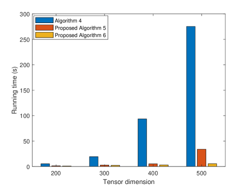
Figure 1: Running time comparison of different algorithms for the synthetics data tensors in Example 1.

6 Experimental Results

In this section, we conduct several simulations to show the efficiency of the proposed algorithms and their superiority over the baseline algorithm. We have used Matlab and some functions of the toolbox:
https://github.com/canyilu/Tensor-tensor-product-toolbox to implement the proposed algorithms using a laptop computer with 2.60 GHz Intel(R) Core(TM) i7-5600U processor and 8GB memory. The algorithms are compared in terms of running time and relative error defined as follows

$${\rm Relative\,\,Error}=\frac{\|\underline{\mathbf{X}}-\underline{\mathbf{U}}*\underline{\mathbf{C}}*\underline{\mathbf{Z}}\|_{F}+\|\underline{\mathbf{Y}}-\underline{\mathbf{V}}*\underline{\mathbf{S}}*\underline{\mathbf{Z}}\|_{F}}{\|\underline{\bf X}\|_{F}+\|\underline{\bf Y}\|_{F}}.$$

The Peak Signal-to-Noise Ratio (PSNR) is also used to compare the quality of images. The PSNR of two images $\underline{\bf X}$ and $\underline{\bf Y}$ is defined as

$${\rm PSNR}=10\log 10\left({\frac{{\|\underline{\bf X}\|}_{\infty}}{\|\underline{\bf X}-\underline{\bf Y}\|_{F}}}\right)\quad{\rm dB}.$$

Example 1.

(Synthetics data tensors) Let us generate random data tensors $\underline{\bf X}$ and $\underline{\bf Y}$ with zero mean and unit variance of size $n\times n\times n$ with the tubal rank 50, where $n=200,300,400,500$. Then, the basic TGSVD and two proposed randomized TGSVD algorithms (Algorithms 6 and 6) are applied to the mentioned data tensor. We set the oversampling as $50$ in both Algorithms 6 and 7. The running times of the algorithms are shown in Figure 1 and the corresponding relative errors achieved by them are reported in Table 1. From Figure 1, for $n=300,400,500$ we achieve $\times 55,\,\times 37.9,$ and $\times 11.01$ speed-up, respectively. So, in all scenarios, we have more than one order of magnitude acceleration. Also from Table 1, we see that the difference between the relative errors of the algorithms is negligible. So, we can provide satisfying results, in much less time than the baseline algorithm 5. This shows the superiority of the proposed algorithms compared to the baseline methods for handling large-scale data tensors.

Table 1: Relative error comparison of different algorithms for the synthetics data tensors in Example 1.

	$n=300$	$n=400$	$n=500$
Algorithm 5	9.8833e-19	6.7230e-19	7.4645e-19
Proposed Algorithm 6	5.4381e-18	2.4254e-18	2.4809e-18
Proposed Algorithm 7	9.8108e-18	9.5354e-18	2.2562e-18

Example 2.

(Synthetics data tensors) In this example, we consider the following data tensors

• $\underline{\bf X}(i,j,k)=\frac{1}{\sqrt{i^{2}+j^{2}+k^{2}}}$

• $\underline{\bf Y}(i,j,k)=\frac{1}{(i^{3}+j^{3}+k^{3})^{1/3}}$

It is easy to check that these tensors have low tubal-rank structures. We set the oversampling parameter to $50$ and the tubal rank $R=50$ in Algorithms 6 and 7 and apply them to the mentioned data tensors. The execution times of the proposed algorithms and the baseline Algorithm 5 are reported in Figure 2. Also, the relative errors of the algorithms are shown in Figure 3. The numerical results presented in Figures 2 and 3, show that Algorithm 7 is much faster than Algorithm 6. We see that the proposed algorithms scale well to the dimension of the data tensors. The accuracy achieved by the proposed algorithms was also almost the same and even better than the baseline algorithm (Algorithm 5), so this indicates the better performance and efficiency of the proposed algorithms.

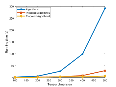
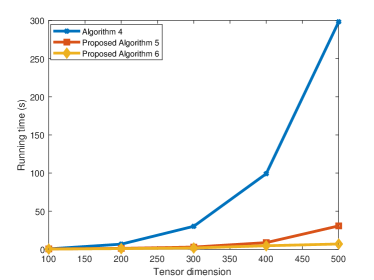
Figure 2: Running time comparison of different algorithms for the synthetics data tensors in Example 2.

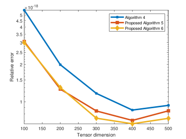
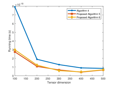
Figure 3: Relative error comparison of the algorithms for the synthetics data tensors in Example 2

Example 3.

(Real data tensors). In this example, we show an application of the proposed algorithms in image restoration task. Image restoration is a computer vision task that involves repairing or improving the quality of damaged or degraded images. The goal of image restoration is to recover the original information, enhance the visual appearance, or remove unwanted artifacts from an image. Let us consider the tensor regularized problem as

$$\min_{\underline{\bf X}\in\mathbb{R}^{m\times 1\times n}}\|\underline{\bf}\underline{\bf A}*\underline{\bf}\underline{\bf X}-\underline{\bf B}\|+\lambda\|\underline{\bf L}*\underline{\bf X}\|,$$ (26)

where $\underline{\bf}\underline{\bf L}\in\mathbb{R}^{s\times m\times n}$ is a regularized operator and $\lambda$ is a regularized parameter. The regularized operator defined as follows

$$\underline{\bf L}(:,:,1)=\frac{1}{4}\begin{bmatrix}-1&2&-1&&\\ &\ddots&\ddots&\ddots&\\ &&-1&2&-1\end{bmatrix},$$ (27)

and the other frontal slices are equal to zero. It is known that this formulation can remove noise and artifacts from images, see [31] for the details about this formulation. The normal equation associated to (26) is

$$(\underline{\bf A}^{T}*\underline{\bf A}+\lambda\underline{\bf L}^{T}*\underline{\bf L})*\underline{\bf X}=\underline{\bf A}^{T}*\underline{\bf B},$$ (28)

and inserting the TGSVD of $\underline{\bf A}$ and $\underline{\bf L}$ in (28)

$$\underline{\bf A}=\underline{\bf U}*\underline{\bf C}*\underline{\bf Z},\quad\underline{\bf L}=\underline{\bf V}*\underline{\bf S}*\underline{\bf Z},$$ (29)

we get the regularized solution as

$$\underline{\bf X}_{\mu}=\underline{\bf Z}^{-1}*(\underline{\bf C}^{T}*\underline{\bf C}+\lambda^{-1}\underline{\bf S}^{T}*\underline{\bf S})^{-1}*\underline{\bf S}^{T}*\underline{\bf U}^{T}*\underline{\bf B}.$$ (30)

To compute the regularized TGSVD, the computation of the GTSVD is required in (29). So, we applied the proposed randomized GTSVD algorithms 6 and 7 and the classical one 5. We considered the “Airplaane”, “Barbara” and “Peppers” images depicted in Figure 4 all are of size $256\times 256\times 3$. Then, we added a noise to the image as

$$\underline{\bf X}=\underline{\bf X}_{clean}+\delta*\frac{\underline{\bf Y}}{\|\underline{\bf Y}\|}\|\underline{\bf X}\|,$$ (31)

where $\underline{\bf Y}$ is a random tensor of size $256\times 256\times 3$. Then the formulation 26 was used for the denoising procedure with the regularized paramter $\lambda=8.56e-2$. The simulation results are reported in Table 2. The numerical results clearly show that the proposed randomized GTSVD algorithms provide satisfying results in much less time compared to the classical GTSVD algorithm. This example convinced us the randomized GTSVD are more efficient and faster in real application scenarios.

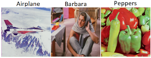
Figure 4: (Top) The true benchmark images for Example 3.

Table 2: The comparison of the PSNR and running time achieved by the proposed algorithms and the baseline method for example 3.

PSNR
Method	Airplane	Barbara	Peppers
Proposed Algorithm 6	27.13	25.76	28.33
Proposed Algorithm 7	27.14	25.78	28.35
Algorithm 5	28.32	26.12	28.89
Time (Second)
Proposed Algorithm 6	2.32	2.11	2.11
Proposed Algorithm 7	2.60	2.45	2.52
Algorithm 5	4.12	4.30	4.24

7 Conclusion and future works

In this paper, we proposed two fast randomized algorithms to compute the generalized T-SVD (GTSVD) of tensors based on the tubal product (t-product). Given two third-order tensors, the random projection technique is first used to compute two small tensor sketches of the given tensors capturing the most important ranges of them. Then from the small sketches, we recovered the GTSVDs of the original data tensor from the GTSVD of the small tensor sketches, which are easier to analyze. The computer simulations were conducted convincing the feasibility and applicability of the proposed randomized algorithm. The error analysis of the proposed algorithms using the power iteration needs to be investigated and this will be our future research. We plan to also develop randomized algorithms for the computation of the GTSVD to be applicable for steaming data tensors, which arises in real-world applications. The generalization of the proposed algorithm to higher order tensors is our ongoing research work.

8 Conflict of Interest Statement

The author declares that he has no conflict of interest with anything.

References

- [1] G. H. Golub, C. F. Van Loan, Matrix computations, JHU press, 2013.
- [2] C. F. Van Loan, Generalizing the singular value decomposition, SIAM Journal on numerical Analysis 13 (1) (1976) 76–83.
- [3] C. C. Paige, M. A. Saunders, Towards a generalized singular value decomposition, SIAM Journal on Numerical Analysis 18 (3) (1981) 398–405.
- [4] P. C. Hansen, Rank-deficient and discrete ill-posed problems: numerical aspects of linear inversion, SIAM, 1998.
- [5] O. Alter, P. O. Brown, D. Botstein, Generalized singular value decomposition for comparative analysis of genome-scale expression data sets of two different organisms, Proceedings of the National Academy of Sciences 100 (6) (2003) 3351–3356.
- [6] S. P. Ponnapalli, M. A. Saunders, C. F. Van Loan, O. Alter, A higher-order generalized singular value decomposition for comparison of global mrna expression from multiple organisms, PloS one 6 (12) (2011) e28072.
- [7] N. Halko, P.-G. Martinsson, J. A. Tropp, Finding structure with randomness: Probabilistic algorithms for constructing approximate matrix decompositions, SIAM review 53 (2) (2011) 217–288.
- [8] W. Wei, H. Zhang, X. Yang, X. Chen, Randomized generalized singular value decomposition, communications on Applied mathematics and computation 3 (1) (2021) 137–156.
- [9] A. K. Saibaba, J. Hart, B. van Bloemen Waanders, Randomized algorithms for generalized singular value decomposition with application to sensitivity analysis, Numerical Linear Algebra with Applications 28 (4) (2021) e2364.
- [10] S. Ahmadi-Asl, A. Cichocki, A. H. Phan, M. G. Asante-Mensah, M. M. Ghazani, T. Tanaka, I. Oseledets, Randomized algorithms for fast computation of low rank tensor ring model, Machine Learning: Science and Technology 2 (1) (2020) 011001.
- [11] S. Ahmadi-Asl, S. Abukhovich, M. G. Asante-Mensah, A. Cichocki, A. H. Phan, T. Tanaka, I. Oseledets, Randomized algorithms for computation of Tucker decomposition and higher order SVD (HOSVD), IEEE Access 9 (2021) 28684–28706.
- [12] M. Che, Y. Wei, Randomized algorithms for the approximations of Tucker and the tensor train decompositions, Advances in Computational Mathematics 45 (1) (2019) 395–428.
- [13] S. Ahmadi-Asl, A randomized algorithm for tensor singular value decomposition using an arbitrary number of passes, arXiv preprint arXiv:2207.12542 (2022).
- [14] J. Zhang, A. K. Saibaba, M. E. Kilmer, S. Aeron, A randomized tensor singular value decomposition based on the t-product, Numerical Linear Algebra with Applications 25 (5) (2018) e2179.
- [15] R. Minster, A. K. Saibaba, M. E. Kilmer, Randomized algorithms for low-rank tensor decompositions in the Tucker format, SIAM Journal on Mathematics of Data Science 2 (1) (2020) 189–215.
- [16] M. E. Kilmer, K. Braman, N. Hao, R. C. Hoover, Third-order tensors as operators on matrices: A theoretical and computational framework with applications in imaging, SIAM Journal on Matrix Analysis and Applications 34 (1) (2013) 148–172.
- [17] M. E. Kilmer, C. D. Martin, Factorization strategies for third-order tensors, Linear Algebra and its Applications 435 (3) (2011) 641–658.
- [18] L. R. Tucker, et al., The extension of factor analysis to three-dimensional matrices, Contributions to mathematical psychology 110119 (1964).
- [19] L. R. Tucker, Some mathematical notes on three-mode factor analysis, Psychometrika 31 (3) (1966) 279–311.
- [20] F. L. Hitchcock, The expression of a tensor or a polyadic as a sum of products, Journal of Mathematics and Physics 6 (1-4) (1927) 164–189.
- [21] F. L. Hitchcock, Multiple invariants and generalized rank of a p-way matrix or tensor, Journal of Mathematics and Physics 7 (1-4) (1928) 39–79.
- [22] Z.-H. He, M. K. Ng, C. Zeng, Generalized singular value decompositions for tensors and their applications., Numerical Mathematics: Theory, Methods & Applications 14 (3) (2021).
- [23] Y. Zhang, X. Guo, P. Xie, Z. Cao, CS decomposition and GSVD for tensors based on the t-product, arXiv preprint arXiv:2106.16073 (2021).
- [24] A. Cichocki, N. Lee, I. Oseledets, A.-H. Phan, Q. Zhao, D. P. Mandic, et al., Tensor networks for dimensionality reduction and large-scale optimization: Part 1 low-rank tensor decompositions, Foundations and Trends® in Machine Learning 9 (4-5) (2016) 249–429.
- [25] C. Lu, J. Feng, Y. Chen, W. Liu, Z. Lin, S. Yan, Tensor robust principal component analysis with a new tensor nuclear norm, IEEE transactions on pattern analysis and machine intelligence 42 (4) (2019) 925–938.
- [26] C. D. Martin, R. Shafer, B. LaRue, An order-p tensor factorization with applications in imaging, SIAM Journal on Scientific Computing 35 (1) (2013) A474–A490.
- [27] W. Yu, Y. Gu, Y. Li, Efficient randomized algorithms for the fixed-precision low-rank matrix approximation, SIAM Journal on Matrix Analysis and Applications 39 (3) (2018) 1339–1359.
- [28] U. O. Ugwu, L. Reichel, Tensor regularization by truncated iteration: a comparison of some solution methods for large-scale linear discrete ill-posed problem with a t-product, arXiv preprint arXiv:2110.02485 (2021).
- [29] U. O. Ugwu, Viterative tensor factorization based on Krylov subspace-type methods with applications to image processing, Kent State University, PhD Thesis,, 2021.
- [30] S. Ahmadi-Asl, An efficient randomized fixed-precision algorithm for tensor singular value decomposition, Communications on Applied Mathematics and Computation (2022) 1–20.
- [31] L. Reichel, U. O. Ugwu, Tensor arnoldi–tikhonov and gmres-type methods for ill-posed problems with a t-product structure, Journal of Scientific Computing 90 (2022) 1–39.