Set-Type Belief Propagation with Applications to Poisson Multi-Bernoulli SLAM

Abstract

Belief propagation (BP) is a useful probabilistic inference algorithm for efficiently computing approximate marginal probability densities of random variables. However, in its standard form, BP is only applicable to the vector-type random variables with a fixed and known number of vector elements, while certain applications rely on random finite sets with an unknown number of vector elements. In this paper, we develop BP rules for factor graphs defined on sequences of RFSs where each RFS has an unknown number of elements, with the intention of deriving novel inference methods for RFSs. Furthermore, we show that vector-type BP is a special case of set-type BP, where each RFS follows the Bernoulli process. To demonstrate the validity of developed set-type BP, we apply it to the Poisson multi-Bernoulli (PMB) filter for simultaneous localization and mapping (SLAM), which naturally leads to new set-type BP-mapping, SLAM, multi-target tracking, and simultaneous localization and tracking filters. Finally, we explore the relationships between the vector-type BP and the proposed set-type BP PMB-SLAM implementations and show a performance gain of the proposed set-type BP PMB-SLAM filter in comparison with the vector-type BP-SLAM filter.

I Introduction

bp is a powerful statistical inference algorithm, applicable to different fields including signal processing, robotics, autonomous vehicles, image processing, and artificial intelligence. In particular, belief propagation (BP) is attractive for computing probability densities in Bayesian networks [1, 2, 3, 4], where one can efficiently compute the marginal probability densities of random variables of interest given the observed data. bp has been actively applied in localization [5, 6], mapping [7], multiple-target tracking (MTT) [8, 9], SLAM [10, 11, 12, 13, 14], and simultaneous localization and tracking (SLAT) [15]. Mapping and MTT respectively involve mapping landmarks and tracking targets, based on the noisy sensor measurements. Simultaneously estimating the unknown sensor state as well as landmarks and targets leads to SLAM and SLAT, respectively. The main challenge in this research stems from the data association uncertainty between the unknown number of targets and imperfect measurements by missed detections and clutter. To effectively address this challenge, several approaches have been developed as follows. Classical SLAM methods [16, 17, 18, 19, 20] consider the data associations outside the Bayesian filter, while the filter operates on vector random variables. With the introduction of RFSs in [21, 22], a theoretically sound tool for modeling the unknown number of targets and for handling the data association between targets and measurements became available. By modeling targets with vector-type random variables, the marginal densities for targets are efficiently computed by BP, relying on several ad-hoc modifications [12, 13, 14]. Between them, the RFS- and BP-based methods have rigorously handled the main challenge of MTT and SLAM by starting with the formulation of joint posterior density of targets and data association.

There are several RFS-based methods for MTT and SLAM. The probability hypothesis density (PHD) [23, 21, 22, 24] and cardinalized probability hypothesis density (CPHD) [25] filters approximate the multi-target posterior as a Poisson point process (PPP), leading to a computationally efficient solution. A more accurate solution can be obtained with RFS filters based on multi-object conjugate priors, which are inherently closed under prediction and update [26, 27, 28, 29]. The Poisson multi-Bernoulli mixture (PMBM) [27, 28] adopts the Poisson birth model and multi-Bernoulli mixture (MBM). For standard multi-object models with Poisson birth [21], the Bayesian optimal solutions to MTT and SLAM are given by the PMBM conjugate prior [26, 28]. With the multi-Bernoulli (MB) birth model instead of Poisson, the conjugate prior is an MBM [27]. The MBM filter corresponds to a PMBM filter where the Poisson intensity equals to zero, and the birth Bernoulli components are added into the MBM in the prediction step. If we expand the number of global hypotheses in the MBM filter such that each Bernoulli has deterministic target existence, we obtain the MBM₀₁ filter [27]. Both MBM and MBM₀₁ filters can be labeled without changing the filtering recursion. The MBM₀₁ filter recursion is analogous to the $\delta$-generalized labeled multi-Bernoulli ($\delta$-GLMB) filtering recursion [30, 31, 32, 33, 34]. Some RFS-based methods rely on BP to compute marginal association probabilities [26], which converts the PMBM [27, 28] to a PMB [26, 35, 29, 28] after every update, by marginalizing out the association variables.

In addition to RFS-based methods, vector-type BP methods have also been applied to tracking and mapping problems. In [8, 9], the MTT problem is tackled by running vector-type BP on the factor graph representation of the joint distribution of target states and data association variables. Here targets are modeled by augmented vectors including the binary target existence indicators, and message passing between targets and data association variables is adopted from [9]. The SLAM problems with radio signal propagation are formulated in [10, 11, 12, 13, 14]. The authors of [10, 11] formulate the factor graph and introduce an efficient message passing scheduling, among the unknown sensor variables consisting of position, orientation, and clock bias, and multiple-types of targets are further studied in [11]. With the augmented target vectors and the factorized joint distribution of targets and data association variables from [9], the message passing methods for joint SLAM and data association are developed [12, 13, 14]. These vector-type BP-based approaches [12, 13, 14] can be explained as the track-oriented PMB filter [28] and yield competitive performance. To handle undetected targets and newly detected targets, the auxiliary PHD is adopted in [12, 13, 14], which was initially considered in [36] for vector-type MTT and in [37] for set-type MTT. However, undetected targets and their connections to newly detected targets are not represented in the formulated factor graph, and corresponding message-passing steps are not explicitly implemented. The modeling of undetected targets in vector-based methods is treated in [38] but the distinction between eventually and never detected targets is required. Moreover, it is not explicitly revealed how to apply BP in the multiple hypotheses tracking formalism. Hence, while BP-based methods have benefits in algorithm implementation, they require certain ad-hoc modifications.

In this paper, we aim to bridge the gap between RFS theory and BP, by developing a novel BP algorithm, running on factor graphs defined on the sequence of RFSs. Like conventional BP, this opens the door to automated inference over factor graphs, once the RFS density is factorized. This approach can avoid the need for heuristics and approximations. Related work has been done in [39], where BP is applied to only the update step, without a systematic treatment to the entire filtering recursion, except for the modeling of undetected targets and newly detected targets. The goal of this paper is thus to formalize set-type BP and the corresponding factor graphs from the RFS densities. From the newly proposed set-type BP, we derive the PMB filter using the developed set-type BP which is applicable to mapping, MTT, SLAM, and SLAT. The contributions of this paper are summarized as follows:

• The specification of set-type BP: We derive set-type BP and demonstrate that vector-type BP is a special case of set-type BP. We also show that as in vector-type BP, the interior stationary points of the constrained Bethe free energy are set-type BP fixed points.

• The introduction of novel factors for set-type BP: We devise a partition and merging factor, which partitions a single set into multiple sets and merges multiple sets into a single set, useful for handling sets with unknown cardinalities. We also propose a conversion factor for sets augmented with auxiliary vectors such as unique marks.

• Derivation of PMB and MB filters with set-type BP for the related problems of mapping, MTT, SLAM, SLAT: With the developed set-type BP, we revisit the PMB- and MB-SLAM filters by factorizing their joint SLAM and data association distribution, formulating a factor graph from the factorized density, and running set-type BP on the factor graph. This work can also lead to set-type BP PMB-mapping, MTT, and SLAT filters. The resulting methods bear close resemblance to the PMB-SLAM filter [28] that computes the marginals, but without its approximations and heuristics.

• Relation to vector-type BP SLAM: We clearly show the connections between the proposed set-type BP PMB-SLAM and vector-type BP-SLAM [12, 13, 14] filters. While the methods turn out to be similar, vector-type BP-SLAM requires heuristics as part of the algorithm development, which is avoided in the proposed set-type BP PMB-SLAM filter. The simulation results show that the proposed set-type BP PMB-SLAM filter outperforms the vector-type BP-SLAM filter [12, 13, 14], especially in scenarios with informative PPP birth.

This paper is organized as follows. Section II provides the background of vector-type BP and RFSs. In Section III, the set-type BP rules and set-type factor nodes are proposed. Proposed set-type BP is applied to the PMB filter, and the connections between set-type and vector-type BP-SLAM filters are analyzed in Section IV. The numerical results and discussions are reported in Section V, and conclusions are drawn in Section VI.

II Background

In this section, we review factor graphs and belief propagation, and we recall the RFS approaches.

Notations: Scalars are denoted by italic font, vectors and matrices are respectively indicated by bold lowercase and uppercase letters, and sets are displayed in calligraphic font, e.g., $x$, $\mathbf{x}$, $\mathbf{X}$, and $\mathcal{X}$. The set of finite subsets of a space $\mathbb{R}$ is denoted by $\mathcal{F}(\mathbb{R})$. The vector consisting of a sequence of vectors $\mathbf{x}^{i}$ is denoted by $\underline{\mathbf{x}}$, and the sequence of multiple sets $\mathcal{X}$ is denoted by $\underline{\mathcal{X}}$.

II-A Vector-Type Factor Graph and Belief Propagation

II-A1 Joint Density Factorization and Factor Graph

Let $\mathbf{x}^{i}\in\mathbb{R}^{n_{\mathbf{x}}}$ denote a single state vector and $\underline{\mathbf{x}}=[(\mathbf{x}^{1})^{\top},\dots,(\mathbf{x}^{N})^{\top}]^{\top}$ denote augment single state vectors representing $N$ states. Then, we denote a joint probability density of the hidden variables $\underline{\mathbf{x}}$ by $f(\underline{\mathbf{x}})$, which can be factorized as [1, 4]

$$f(\underline{\mathbf{x}})\propto\prod_{a}f_{a}(\underline{\mathbf{x}}^{a}),$$ (1)

where $f_{a}(\underline{\mathbf{x}}^{a})$ denotes a nonnegative function, and $\underline{\mathbf{x}}^{a}$ denotes the argument vector of the function $f_{a}(\cdot)$.

The factorized functions in (1) and corresponding argument vectors can be represented by a factor graph. The factor graph with the general graphical model [1] consists of nodes for the different factors and variables, illustrated by squares for the factors, $f_{a}(\cdot)$, and circles for the variables, $\mathbf{x}^{i}$, respectively, with edge connections between the factors and their argument variables.

Example 1.

Suppose we have a probability density $f(\underline{\mathbf{x}})$, such that $\underline{\mathbf{x}}=[(\mathbf{x}^{1})^{\top},(\mathbf{x}^{2})^{\top}]^{\top}$, $\underline{\mathbf{x}}^{A}=\mathbf{x}^{1}$, $\underline{\mathbf{x}}^{B}=\mathbf{x}^{2}$, $\underline{\mathbf{x}}^{C}=[(\mathbf{x}^{1})^{\top},(\mathbf{x}^{2})^{\top}]^{\top}$, which can be factorized as

$$f(\underline{\mathbf{x}})\propto f_{A}(\mathbf{x}^{1})f_{B}(\mathbf{x}^{2})f_{C}(\mathbf{x}^{1},\mathbf{x}^{2}).$$ (2)

The corresponding factor graph is illustrated in Fig. 1.

Figure 1: Factor graph representation of the factorized vector density (2).

II-A2 Belief Propagation

bp is an efficient approach for estimating the marginal densities of the variables from a joint probability density function [1]. By running BP on the factor graph, we compute the messages passed between factors and variables for all links. We denote the propagated messages from factor $a$ to variable $i$ and from variable $i$ to factor $a$ by $\mathtt{m}_{a\to i}(\mathbf{x}^{i})$ and $\mathtt{n}_{i\to a}(\mathbf{x}^{i})$, respectively. The messages are updated with the following rules:

$$\mathtt{m}_{a\to i}(\mathbf{x}^{i}) =\int f_{a}(\underline{\mathbf{x}}^{a})\prod_{j\in\mathcal{N}(a)\setminus\{i\}}\mathtt{n}_{j\to a}(\mathbf{x}^{j})\mathrm{d}\mathbf{x}^{\sim i},$$ (3)

$$\mathtt{n}_{i\to a}(\mathbf{x}^{i}) =\prod_{b\in\mathcal{M}(i)\setminus\{a\}}\mathtt{m}_{b\to i}(\mathbf{x}^{i}),$$ (4)

where $\mathcal{N}(a)$ denotes the set of indices $i$ of neighboring vectors linked to the factor $f_{a}(\underline{\mathbf{x}}^{a})$, such that $i\in\mathcal{N}(a)$ if and only if $\mathbf{x}^{i}$ is an argument of $f_{a}(\cdot)$, $\mathcal{M}(i)$ denotes the set of indices $a$ of neighboring factors linked to the variable $\mathbf{x}^{i}$, such that $a\in\mathcal{M}(i)$ if and only if $\mathbf{x}^{i}$ is an argument of $f_{a}(\cdot)$, and $\int\dots\mathrm{d}\mathbf{x}^{\sim i}$ denotes integration with respect to all vectors $\mathbf{x}^{j}$ except $\mathbf{x}^{i}$. The messages can be used to compute beliefs that approximate the marginalized posterior densities. The beliefs at variable $i$ and factor $a$ are denoted $\mathtt{b}(\mathbf{x}^{i})$ and $\mathtt{b}(\underline{\mathbf{x}}^{a})$, respectively, and are updated using the following rules:

$$\mathtt{b}(\mathbf{x}^{i}) \propto\prod_{a\in\mathcal{M}(i)}\mathtt{m}_{a\to i}(\mathbf{x}^{i}),$$ (5)

$$\mathtt{b}(\underline{\mathbf{x}}^{a}) \propto f_{a}(\underline{\mathbf{x}}^{a})\prod_{i\in\mathcal{N}(a)}\mathtt{n}_{i\to a}(\mathbf{x}^{i}).$$ (6)

II-B Random Finite Sets

II-B1 Set-Variables, Density, and Integral

Let us denote an RFS by $\mathcal{X}=\{\mathbf{x}^{1},\dots,\mathbf{x}^{n}\}\in\mathcal{F}(\mathbb{R}^{n_{\mathbf{x}}})$, where both vector $\mathbf{x}^{i}$, $i\in\{1,\dots,n\}$ and cardinality ${n}=\lvert\mathcal{X}\rvert$ are random. We define a set-density $f({\mathcal{X}})$ as [26]

$$f({\mathcal{X}})=p(n)\sum_{\pi}f^{n}({\mathbf{x}}^{\pi(1)},\dots,{\mathbf{x}}^{\pi(n)}),$$ (7)

in which $p(n)=\mathrm{Pr}(\lvert{\mathcal{X}}\rvert=n)$ denotes the probability mass function of the set cardinality, $\pi$ denotes a possible permutation of the set $\mathcal{N}=\{1,\dots,n\}$ with $\pi(i)\in\mathcal{N}$, and $f^{n}(\cdot)$ is the joint probability density function of the vector with $n$ elements, evaluated for permutation $\pi$. Given the set-valued function $g(\cdot)$, we define the set integral as [22, eq. (3.11)]

$$\int g({\mathcal{X}})\delta{\mathcal{X}}=g(\emptyset)+\sum_{n=1}^{\infty}\dfrac{1}{n!}\int g(\{{\mathbf{x}}^{1},\dots,{\mathbf{x}}^{n}\})\mathrm{d}{\mathbf{x}}^{1}\dots\mathrm{d}{\mathbf{x}}^{n}.$$ (8)

II-B2 Poisson, Bernoulli, and PMB Densities

We will follow the definitions from [21]. Suppose we have a set $\mathcal{X}^{\mathrm{U}}$ that follows the Poisson process. The density is given by [26]

$$f^{\mathrm{PPP}}(\mathcal{X}^{\mathrm{U}})=e^{-\int\lambda(\mathbf{x})\mathrm{d}\mathbf{x}}\prod_{\mathbf{x}\in\mathcal{X}^{\mathrm{U}}}\lambda(\mathbf{x}),$$ (9)

where $\lambda(\mathbf{x})$ denotes the Poisson intensity function. A Bernoulli density $f^{\mathrm{B}}(\mathcal{X})$ is given by

$$f^{\mathrm{B}}(\mathcal{X})=\begin{cases}1-r,&\mathcal{X}=\emptyset\\ r\,f(\mathbf{x}),&\mathcal{X}=\{\mathbf{x}\}\\ 0,&\lvert\mathcal{X}\rvert>1,\end{cases}$$ (10)

where $f(\mathbf{x})$ and $r\in[0,1]$ denote the spatial density and the existence probability, respectively. An MB density with $n$ Bernoulli components is given by

$$f^{\mathrm{MB}}(\mathcal{X}^{\mathrm{D}}) =\sum_{\uplus_{i=1}^{n}\mathcal{X}^{i}=\mathcal{X}^{\mathrm{D}}}\,\,\,\prod_{i=1}^{n}f^{i}(\mathcal{X}^{i}),$$ (11)

where $f^{i}(\mathcal{X}^{i})$ is a Bernoulli density, and $\uplus$ stands for disjoint set union [40, pp. 24].

We are now ready to introduce a PMB density, defined as follows. Suppose we have two independent RFSs $\mathcal{X}^{\mathrm{U}}$ and $\mathcal{X}^{\mathrm{D}}$ such that $\mathcal{X}=\mathcal{X}^{\mathrm{U}}\uplus\mathcal{X}^{\mathrm{D}}$, where $\mathcal{X}^{\mathrm{D}}$ follows a MB process and $\mathcal{X}^{\mathrm{U}}$ follows a PPP. Using the convolution formula for independent RFSs [21], a PMB density $f(\mathcal{X})$ is

$$f^{\mathrm{PMB}}(\mathcal{X})\propto\sum_{\uplus_{i=1}^{n}\mathcal{X}^{i}\uplus\mathcal{X}^{\mathrm{U}}=\mathcal{X}}\,\,\prod_{\mathbf{x}\in\mathcal{X}^{\mathrm{U}}}\lambda(\mathbf{x})\prod_{i=1}^{n}f^{i}(\mathcal{X}^{i}).$$ (12)

II-B3 Auxiliary Variables

The derivation of set-type BP PMB filters will require us to introduce auxiliary variables to remove the summation in (12). In particular, we introduce $u\in\mathbb{U}$ in the PMB density (12), where $\mathbb{U}=\{0,1,\dots,n\}$  [41, 39]. We thus extend the single state space, such that $({u},\mathbf{x})\in\mathbb{U}\times\mathbb{R}^{n_{\mathbf{x}}}$, and denote a set of target states with auxiliary variables by $\tilde{\mathcal{X}}\in\mathcal{F}(\mathbb{U}\times\mathbb{R}^{n_{\mathbf{x}}})$. The set with the auxiliary variable ${u}=0$ follows a PPP and indicates that the targets have not been detected, denoted by $\tilde{\mathcal{X}}^{\mathrm{U}}=\{(u,\mathbf{x})\in\tilde{\mathcal{X}}:u=0\}$. Similarly, the set with ${u}=i$ follows a Bernoulli process and indicates that the single target has previously been detected, denoted by $\tilde{\mathcal{X}}^{i}=\{(u,\mathbf{x})\in\tilde{\mathcal{X}}:u=i\}$. For the set of targets with auxiliary variables $\tilde{\mathcal{X}}$, the PMB density is [41, Definition 1]

$$\tilde{f}^{\mathrm{PMB}}(\tilde{\mathcal{X}}) =\tilde{f}^{\mathrm{U}}(\tilde{\mathcal{X}}^{\mathrm{U}})\prod_{i=1}^{n}\tilde{f}^{i}(\tilde{\mathcal{X}}^{i}).$$ (13)

Here $\tilde{f}^{\mathrm{U}}(\tilde{\mathcal{X}}^{\mathrm{U}})$ and $\tilde{f}^{i}(\tilde{\mathcal{X}}^{i})$ are given by

$$\tilde{f}^{\mathrm{U}}(\tilde{\mathcal{X}}^{\mathrm{U}}) =\exp\left(-\int\lambda(\mathbf{x})\mathrm{d}\mathbf{x}\right)\prod_{(u,\mathbf{x})\in\tilde{\mathcal{X}}^{\mathrm{U}}}\delta_{0}[u]\lambda(\mathbf{x}),$$ (14)

$$\tilde{f}^{i}(\tilde{\mathcal{X}}^{i}) =\begin{cases}1-r^{i},&\tilde{\mathcal{X}}^{i}=\emptyset\\ r^{i}f^{i}(\mathbf{x})\delta_{i}[u],&\tilde{\mathcal{X}}^{i}=(u,\mathbf{x})\\ 0,&\text{otherwise}\end{cases},$$ (15)

where $\delta_{i}[\cdot]$ denotes the Kronecker delta function. For notational simplicity, $\tilde{\cdot}$ on sets with auxiliary variables will be omitted, when possible.

III Factor Graph and Belief Propagation for Random Finite Set

We describe the proposed set-type BP update rules and special factors for RFSs. We reveal that set-type BP is a generalization of standard vector-type BP since a vector can be represented as a set with a single element $p(n=1)=1$ of (7).

III-A Factor Graphs and BP over a Sequence of RFSs

Suppose we have $n$ RFSs ${\mathcal{X}}^{1},\dots,{\mathcal{X}}^{n}$, with the joint density $f({\mathcal{X}}^{1},\dots,{\mathcal{X}}^{n})$. In the general formulation of set-type BP, ${\mathcal{X}}^{1},\dots,{\mathcal{X}}^{n}$ may or may not contain auxiliary variables, and the number of RFSs in the sequence, $n$, is known.

Definition 1 (Factorization of Set-Density and Factor Graph).

Let us denote by $f_{a}(\cdot)$ the set-factor $a$, which is a nonnegative function; by $\mathcal{N}(a)$ the set of neighboring set-variable indices linked to the set-factor $a$; by $\mathcal{X}^{i}$ the set-variable $i$; by $\mathcal{M}(i)$ the set of neighboring set-factor indices linked to the set-variable $\mathcal{X}^{i}$; and by $\underline{\mathcal{X}}^{a}$ the arguments of the set-factor $a$, represented by the sequence of all RFSs $\mathcal{X}^{i}$ for $i\in\mathcal{N}(a)$. Suppose the joint density $f({\mathcal{X}}^{1},\dots,{\mathcal{X}}^{n})$ is factorized as follows:

$$f({\mathcal{X}}^{1},\dots,{\mathcal{X}}^{n})\propto\prod_{a}f_{a}(\underline{\mathcal{X}}^{a}).$$ (16)

The factorized density can then be represented by a factor graph, consisting of the set-variables $\mathcal{X}^{i}$ and set-factors $f_{a}(\underline{\mathcal{X}}^{a})$, which can be represented by circles and squares, and edge connections between $\mathcal{X}^{i}$ and $f_{a}(\underline{\mathcal{X}}^{a})$. It should be noted that $f_{a}(\underline{\mathcal{X}}^{a})$ has adequate units for each cardinality of $\underline{\mathcal{X}}^{a}$ such that we can integrate (16) using set integrals over ${\mathcal{X}}^{1},\dots,{\mathcal{X}}^{n}$ [22, Sec. 3.2.4].

Example 2.

Given a set-density $f(\mathcal{X}^{1},\mathcal{X}^{2})$, such that $\underline{\mathcal{X}}^{A}=\mathcal{X}^{1}$, $\underline{\mathcal{X}}^{B}=\mathcal{X}^{2}$, and $\underline{\mathcal{X}}^{C}=(\mathcal{X}^{1},\mathcal{X}^{2})$, which can be factorized as

$$f({\mathcal{X}}^{1},{\mathcal{X}}^{2})\propto f_{A}(\mathcal{X}^{1})f_{B}(\mathcal{X}^{2})f_{C}(\mathcal{X}^{1},\mathcal{X}^{2}).$$ (17)

Using the set-variables and set-factors, the factor graph corresponding to (17) is shown in Fig. 2.

Figure 2: Factor graph representation of set-density of (17).

Definition 2 (Set-Type BP Update Rules).

The set-messages from the set-factor $a$ to the set-variable $i$ are denoted by $\mathtt{m}_{a\to i}(\mathcal{X}^{i})$, while those from the set-variable $i$ to the set-factor $a$ are denoted by $\mathtt{n}_{i\to a}(\mathcal{X}^{i})$. The beliefs at the set-variable $i$ and set-factor $a$ are denoted by $\mathtt{b}(\mathcal{X}^{i})$ and $\mathtt{b}(\underline{\mathcal{X}}^{a})$, respectively. The set-messages are updated with the following rules:

$$\mathtt{m}_{a\to i}(\mathcal{X}^{i}) =\int f_{a}(\underline{\mathcal{X}}^{a})\prod_{j\in\mathcal{N}(a)\setminus\{i\}}\mathtt{n}_{j\to a}(\mathcal{X}^{j})\delta\mathcal{X}^{\sim i},$$ (18)

$$\mathtt{n}_{i\to a}(\mathcal{X}^{i}) =\prod_{b\in\mathcal{M}(i)\setminus\{a\}}\mathtt{m}_{b\to i}(\mathcal{X}^{i}),$$ (19)

where $\setminus$ denotes the set difference, and $\int\dots\delta\mathcal{X}^{\sim i}$ denotes integration with respect to all sets $\mathcal{X}^{j}$ except $\mathcal{X}^{i}$, i.e., with respect to all $\mathcal{X}^{j}$ for which $j\in\mathcal{N}(a)\setminus\{i\}$. The beliefs at the set-variable $i$ and set-factor $a$ are updated with the following rules:

$$\mathtt{b}(\mathcal{X}^{i}) \propto\prod_{a\in\mathcal{M}(i)}\mathtt{m}_{a\to i}(\mathcal{X}^{i})$$ (20)

$$\mathtt{b}(\underline{\mathcal{X}}^{a}) \propto f_{a}(\underline{\mathcal{X}}^{a})\prod_{i\in\mathcal{N}(a)}\prod_{b\in\mathcal{M}(i)\setminus\{a\}}\mathtt{m}_{b\to i}(\mathcal{X}^{j}).$$ (21)

The optimality of the set-type BP update rules in Definition 1 is described by Theorem 1 and Corollary 1, provided next.

Theorem 1.

The interior stationary points of the constrained Bethe free energy are set-type BP fixed points with positive set-beliefs and vice versa.

Proof.

See Appendix A. ∎

Corollary 1.

The set-beliefs obtained by running set-type BP on a factor graph that has no cycles, represent the exact marginal probability densities.

Proof.

See Appendix B. ∎

Example 3.

Consider the factor graph in Fig. 2, representing the factorized density in Example 2. Using set-type BP, the beliefs at set-variable 1 and factor $C$ are obtained as follows: $\mathtt{m}_{A\rightarrow 1}(\mathcal{X}^{1})=f_{A}(\mathcal{X}^{1})$, $\mathtt{m}_{B\rightarrow 2}(\mathcal{X}^{2})=f_{B}(\mathcal{X}^{2})$, $\mathtt{n}_{1\rightarrow C}(\mathcal{X}^{1})=\mathtt{m}_{A\rightarrow 1}(\mathcal{X}^{1})$, $\mathtt{n}_{2\rightarrow C}(\mathcal{X}^{2})=\mathtt{m}_{B\rightarrow 2}(\mathcal{X}^{2})$,

$$\mathtt{m}_{C\rightarrow 1}(\mathcal{X}^{1}) =\int\mathtt{n}_{2\rightarrow C}(\mathcal{X}^{2})f_{C}(\mathcal{X}^{1},\mathcal{X}^{2})\delta\mathcal{X}^{2},$$ (22a)

$$\mathtt{b}(\mathcal{X}^{1}) \propto\mathtt{m}_{A\rightarrow 1}(\mathcal{X}^{1})\mathtt{m}_{C\rightarrow 1}(\mathcal{X}^{1}),$$ (22b)

$$\mathtt{b}(\mathcal{X}^{C}) \propto f_{C}(\mathcal{X}^{1},\mathcal{X}^{2})\mathtt{m}_{A\rightarrow 1}(\mathcal{X}^{1})\mathtt{m}_{B\rightarrow 2}(\mathcal{X}^{2}).$$ (22c)

Remark 1 (Vector-Type BP is a Special Case of Set-Type BP).

Note that the vector-type BP message passing rules and beliefs can be obtained from the set-type BP expressions when considering sets whose cardinality 1 with probability 1, i.e., $p(\lvert\mathcal{X}^{i}\rvert=1)=1,~{}\forall~{}i$. Note that this property implies that we can directly apply BP to joint set and vector densities using the set- and vector-integrals for set- and vector-variables, respectively. A vector-type factor graph (1) can be written as a set-type factor graph in (16) with the property that each factor requires sets with cardinality 1. Then, for factors that only consider sets with cardinality 1, the set integral is equivalent to a vector integral, and the set-type BP message (20)-(21) becomes equivalent to those in (5)-(6).

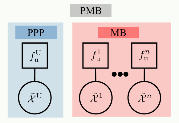
Figure 3: Factor graph of a PMB density with auxiliary variables, see (13), the product of a PPP and $n$ Bernoulli densities.

III-B Examples and Special Factors for Set Densities

III-B1 Factor Graph of a PMB Density

We have so far explained how set-type BP can be applied to a joint density over a sequence of RFSs. We now proceed to explain how to obtain this type of density from a PMB density (12).

A set-density defined in a single-target space that is the disjoint union of different sub-spaces can be used to define a density over a sequence of sets [22, Eq. 3.52]. This type of single-target space was obtained when we introduced auxiliary variables to the PMB in (12), resulting in (13). Therefore, applying this result to the PMB density of the form (13) yields

$$\tilde{f}^{\mathrm{PMB}}(\tilde{\mathcal{X}}^{\mathrm{U}},\tilde{\mathcal{X}}^{1},\dots,\tilde{\mathcal{X}}^{n})=\tilde{f}^{\mathrm{PMB}}(\tilde{\mathcal{X}}^{\mathrm{U}}\uplus\tilde{\mathcal{X}}^{1}\uplus\dots\uplus\tilde{\mathcal{X}}^{n}).$$ (23)

We can now use this joint density over a sequence of RFSs to apply set-type BP. The factor graph of a PMB density (13) with auxiliary variables is then shown in Fig. 3. Since the density is fully factorized, it appears as a collection of disjoint factors. We can also directly obtain the factor graph of a PPP and an MB density with auxiliary variables by removing the required factors and variables in Fig. 3.

III-B2 Partitioning and Merging Factor

Unions of RFSs are common in the literature [22, Sec. 3.5.3]. To represent unions of RFSs in a factor graph, we introduce what we refer to as partitioning and merging factors, defined as follows.

Definition 3 (Partitioning and Merging Factor).

We define a partitioning and merging set-factor as

$$f_{a}(\underline{\mathcal{X}}^{a}) =\delta_{\uplus_{i\in\mathcal{N}(a)\setminus\{j\}}\mathcal{X}^{i}}(\mathcal{X}^{j}),$$ (24)

where $\delta_{\mathcal{X}}(\cdot)$ denotes a set Dirac delta centered at set $\mathcal{X}$, defined in [21, Sec. 11.3.4.3] and $\mathcal{X}^{j}$ is the union $\mathcal{X}^{j}=\uplus_{i\in\mathcal{N}(a)\setminus\{j\}}\mathcal{X}^{i}$. This factor partitions a single set $\mathcal{X}^{j}$ into $\lvert\mathcal{N}(a)\rvert-1$ subsets, i.e., $\mathcal{X}^{i}$ for $i\in\mathcal{N}(a)\setminus\{j\}$, and merges $\lvert\mathcal{N}(a)\rvert-1$ sets, i.e., $\mathcal{X}^{i}$ for $i\in\mathcal{N}(a)\setminus\{j\}$, into a single set $\mathcal{X}^{j}$.

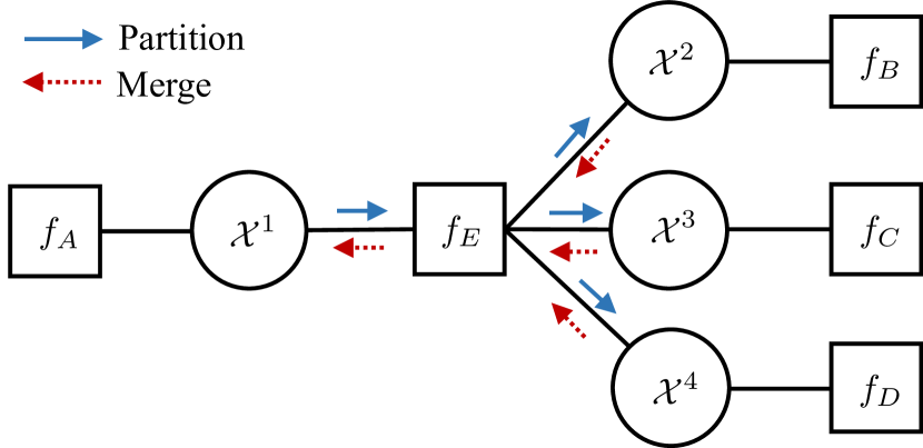
Figure 4: Factor graph representation with a partitioning and merging factor: (left-right) one incoming message is partitioned into multiple messages; and (right-left) multiple messages are merged into one message.

It is useful to understand how this factor affects the set-messages. Suppose we have incoming messages $\mathtt{n}_{j\rightarrow a}(\mathcal{X}^{j})$ and $\mathtt{n}_{q\rightarrow a}(\mathcal{X}^{q})=1$ for $q\in\mathcal{N}(a)\setminus\{j,i\}$. By following the set-type BP update rules, the outgoing messages from the set-factor $a$ to set-variable $i$ for $i\in\mathcal{N}(a)\setminus\{j\}$ are

$$\mathtt{m}_{a\to i}(\mathcal{X}^{i}) =\int\mathtt{n}_{j\to a}(\mathcal{X}^{j})\delta_{\uplus_{q\in\mathcal{N}(a)\setminus\{j\}}\mathcal{X}^{q}}(\mathcal{X}^{j})\delta\mathcal{X}^{\sim i}$$ (25)

$$=\int\mathtt{n}_{j\to a}(\uplus_{q\in\mathcal{N}(a)\setminus\{j\}}\mathcal{X}^{q})\delta\mathcal{X}^{\sim(i,j)}$$ (26)

$$=\int\mathtt{n}_{j\to a}(\mathcal{X}^{i}\uplus\mathcal{X})\delta\mathcal{X},$$ (27)

where $\int\delta\mathcal{X}^{\sim(i,j)}$ indicates the integration with respect to all sets $\mathcal{X}^{q}$ except $\mathcal{X}^{i}$ and $\mathcal{X}^{j}$, and $\mathcal{X}$ is a dummy variable that is used to integrate over all possible sets. It indicates that $\mathcal{X}=\uplus_{q\in\mathcal{N}(a)\setminus\{j,i\}}\mathcal{X}^{q}$, and the single set $\mathcal{X}^{j}$ with the incoming message $\mathtt{n}_{j\to a}(\mathcal{X}^{j})$ is partitioned into $\lvert\mathcal{N}(a)\rvert-1$ subsets $\mathcal{X}^{i}$ with the outgoing messages $\mathtt{m}_{a\rightarrow i}(\mathcal{X}^{i})$, for $i\in\mathcal{N}(a)\setminus\{j\}$.

Conversely, suppose we have incoming messages $\mathtt{n}_{i\to a}(\mathcal{X}^{i})$ for $i\in\mathcal{N}(a)\setminus\{j\}$, then the outgoing message from the set-factor $a$ to the set-variable $j$ is

$$\mathtt{m}_{a\rightarrow j}(\mathcal{X}^{j})$$

$$=\int\prod_{i\in\mathcal{N}(a)\setminus\{j\}}\mathtt{n}_{i\to a}(\mathcal{X}^{i})\delta_{\uplus_{i\in\mathcal{N}(a)\setminus\{j\}}\mathcal{X}^{i}}(\mathcal{X}^{j})\delta\mathcal{X}^{\sim j}$$ (28)

$$=\int\sum_{\uplus_{i\in\mathcal{N}(a)\setminus\{j\}}\mathcal{W}^{i}=\mathcal{X}^{j}}\prod_{i\in\mathcal{N}(a)\setminus\{j\}}\mathtt{n}_{i\to a}(\mathcal{X}^{i})\delta_{\mathcal{W}^{i}}(\mathcal{X}^{i})\delta\mathcal{X}^{\sim j}$$ (29)

$$=\sum_{\uplus_{i\in\mathcal{N}(a)\setminus\{j\}}\mathcal{W}^{i}=\mathcal{X}^{j}}\prod_{i\in\mathcal{N}(a)\setminus\{j\}}\mathtt{n}_{i\to a}(\mathcal{W}^{i}),$$ (30)

where in step (28), we have used that $\delta_{\uplus_{i\in\mathcal{N}(a)\setminus\{j\}}\mathcal{X}^{i}}(\mathcal{X}^{j})=\sum_{\uplus_{i\in\mathcal{N}(a)\setminus\{j\}}\mathcal{W}^{i}=\mathcal{X}^{j}}\prod_{i\in\mathcal{N}(a)\setminus\{j\}}\delta_{\mathcal{W}^{i}}(\mathcal{X}^{i})$ by the convolution formula. Then, (30) indicates that the sets $\mathcal{X}^{i}$ with the incoming messages $\mathtt{n}_{i\to a}(\mathcal{X}^{i})$ for $i\in\mathcal{N}(a)\setminus\{j\}$ are merged into the single set $\mathcal{X}^{j}$ with the outgoing message $\mathtt{m}_{a\to j}(\mathcal{X}^{j})$.

Example 4.

Given the factor graph shown in Fig. 4 such that $\mathcal{X}^{1}=\mathcal{X}^{2}\uplus\mathcal{X}^{3}\uplus\mathcal{X}^{4}$, the argument at the set-factor $E$ is represented as the sequence of sets as $\underline{\mathcal{X}}^{E}=(\mathcal{X}^{1},\mathcal{X}^{2},\mathcal{X}^{3},\mathcal{X}^{4})$ by Definition 1. By Definition 3, the partitioning and merging factor is given by $f_{E}(\underline{\mathcal{X}}^{E})=\delta_{\mathcal{X}^{2}\uplus\mathcal{X}^{3}\uplus\mathcal{X}^{4}}(\mathcal{X}^{1})$. Suppose we have incoming messages $\mathtt{n}_{1\rightarrow E}(\mathcal{X}^{1})$, $\mathtt{n}_{i\rightarrow E}(\mathcal{X}^{i})=1$, for $i\in\{2,3,4\}$. From (26), the partitioned message $\mathtt{m}_{E\rightarrow i}(\mathcal{X}^{i})$ is computed as

$$\mathtt{m}_{E\rightarrow i}(\mathcal{X}^{i}) =\int\mathtt{n}_{1\rightarrow E}(\mathcal{X}^{2}\uplus\mathcal{X}^{3}\uplus\mathcal{X}^{4})\delta\mathcal{X}^{\sim(i,1)},$$ (31)

for $i=2,3,4$. Conversely, suppose we have incoming messages $\mathtt{n}_{j\rightarrow E}(\mathcal{X}^{j})$ for $j\in\{2,3,4\}$, then the outgoing message from the set-factor $E$ to set-variable 1 is computed as

$$\mathtt{m}_{E\rightarrow 1}(\mathcal{X}^{1})$$

$$=\sum_{\mathcal{W}^{2}\uplus\mathcal{W}^{3}\uplus\mathcal{W}^{4}=\mathcal{X}^{1}}\mathtt{n}_{2\rightarrow E}(\mathcal{W}^{2})\ \mathtt{n}_{3\rightarrow E}(\mathcal{W}^{3})\mathtt{n}_{4\rightarrow E}(\mathcal{W}^{4}).$$ (32)

That is, the outgoing message is the convolution of the three incoming messages, representing the union of three independent RFSs.

Proposition 1 (PPP Partitioning and Merging).

Suppose we have a set factor $f_{a}(\underline{\mathcal{X}}^{a})$ and an RFS $\mathcal{X}^{j}=\uplus_{i\in\mathcal{N}(a)\setminus\{j\}}\mathcal{X}^{i}$. Let the RFSs $\mathcal{X}^{i}$ for $i\in\mathcal{N}(a)$ follow a Poisson process. From (27), the partitioning messages from $f_{a}(\underline{\mathcal{X}}^{a})$ to $\mathcal{X}^{i}$ with $i\in\mathcal{N}(a)\setminus\{j\}$ are

$$\mathtt{m}_{a\rightarrow i}(\mathcal{X}^{i})\propto f^{\mathrm{PPP}}(\mathcal{X}^{i}),$$ (33)

From (30), the merging messages from $f_{a}(\underline{\mathcal{X}}^{a})$ to $\mathcal{X}^{j}$ is

$$\mathtt{m}_{a\rightarrow j}(\mathcal{X}^{j}) =\sum_{\uplus_{i\in\mathcal{N}(a)\setminus\{j\}}\mathcal{W}^{i}=\mathcal{X}^{j}}\prod_{i\in\mathcal{N}(a)\setminus\{j\}}f^{\mathrm{PPP}}(\mathcal{W}^{i}),$$ (34)

which follows a PPP.

Proof.

See Appendix C. ∎

III-B3 Auxiliary Variable Shifting Factor

We introduce a factor to change the auxiliary variables.

Definition 4 (Auxiliary Variable Shifting Function).

Given an arbitrary integer $L$ and a single-target space with auxiliary variables, such that $({u},\mathbf{x})\in\mathbb{U}\times\mathbb{R}^{n_{\mathbf{x}}}$, we define the function

$$\mathtt{h}_{L}(u,\mathbf{x})=(u+L,\mathbf{x}),$$ (35)

which shifts the auxiliary variables units by $L$. The function $\mathtt{h}_{L}(\cdot)$ can be extended to a set $\tilde{\mathcal{X}}\in\mathcal{F}(\mathbb{U}\times\mathbb{R}^{n_{\mathbf{x}}})$ such that

$$\mathtt{h}_{L}(\tilde{\mathcal{X}})=\uplus_{(u,\mathbf{x})\in\tilde{\mathcal{X}}}\{(u+L,\mathbf{x})\}.$$ (36)

Definition 5 (Conversion Factor for Auxiliary Variables).

We have two sets $\tilde{\mathcal{X}}^{i}=\{({u}^{1},\mathbf{x}^{1}),\dots,({u}^{n},\mathbf{x}^{n})\}$ and $\tilde{\mathcal{X}}^{j}=\{({u}^{1}+L,\mathbf{x}^{1}),\dots,({u}^{n}+L,\mathbf{x}^{n})\}$, where $L$ is an integer. By Definition 4, we define the conversion factor for auxiliary variables as

$$f_{a}(\tilde{\mathcal{X}}^{i},\tilde{\mathcal{X}}^{j})=\delta_{\mathtt{h}_{-L}(\tilde{\mathcal{X}}^{j})}(\tilde{\mathcal{X}^{i}}),$$ (37)

where $\mathtt{h}_{-L}(\cdot)$ is given by (36).

It is useful to understand how this factor affects the set-messages. Suppose we have an incoming message $\mathtt{n}_{i\rightarrow a}(\tilde{\mathcal{X}}^{i})$. Then, the outgoing message from $f_{a}(\tilde{\mathcal{X}}^{i},\tilde{\mathcal{X}}^{j})$ to $\tilde{\mathcal{X}}^{j}$ is

$$\mathtt{m}_{a\rightarrow j}(\tilde{\mathcal{X}^{j}}) =\int\mathtt{n}_{i\rightarrow a}(\tilde{\mathcal{X}}^{i})\delta_{\mathtt{h}_{-L}(\tilde{\mathcal{X}}^{j})}(\tilde{\mathcal{X}}^{i})\delta\tilde{\mathcal{X}}^{i}$$ (38)

$$=\mathtt{n}_{i\rightarrow a}(\mathtt{h}_{-L}(\tilde{\mathcal{X}}^{j}))=\mathtt{n}_{i\rightarrow a}(\tilde{\mathcal{X}}^{i}).$$ (39)

That is, the outgoing message has the same form as the incoming message with the difference that the auxiliary variables of the incoming message have been converted by the auxiliary variable shifting functions.

IV Application of Set-Type Belief Propagation

The aim of this section is to propose an application of the developed set-type BP update rules and special factors for RFSs. In particular, we derive set-type BP PMB and set-type MB filters for SLAM, where the targets and measurements are modeled by RFSs.

IV-A Problem Formulation

IV-A1 Objective

Our objective is to compute the marginal densities $f(\mathbf{s}_{k}|\mathcal{Z}_{1:k})$ and $f(\tilde{\mathcal{X}_{k}}|\mathcal{Z}_{1:k})$ at discrete time $k$, where the random vector $\mathbf{s}_{k}$ denotes a sensor state, the RFS $\tilde{\mathcal{X}_{k}}$ denotes the set of target states with auxiliary variables, modeled by a PMB. To compute the marginal densities, we adopt the sequential Bayesian framework consisting of prediction and update steps, which will be detailed in Section IV-B and IV-C.

IV-A2 Multi-Target Dynamics

Each target $\mathbf{x}_{k-1}\in\tilde{\mathcal{X}}_{k-1}$ at time $k-1$ survives with probability $p_{\mathrm{S}}(\mathbf{x}_{k-1})$ or dies with probability $1-p_{\mathrm{S}}(\mathbf{x}_{k-1})$. The surviving targets evolve with a transition density $f(\cdot|\mathbf{x}_{k-1})$ but may be static (in which case they are landmarks) or mobile (in this case they are targets, which is the terminology we will adopt here). The set of targets at time step $k$, $\tilde{\mathcal{X}}_{k}$, is the union of surviving and evolving targets and new targets, where target birth follows a PPP with the intensity $\lambda_{\mathrm{B}}(\cdot)$. The sensor may have an unknown state (in the case of SLAT and SLAM) or a known state (in the case of MTT and mapping).

IV-A3 Measurements

The targets ${\mathcal{X}}_{k}$ are observed at the sensor state $\mathbf{s}_{k}$, and the observations are denoted using a measurement set $\mathcal{Z}_{k}$. Each target $\mathbf{x}_{k}\in\tilde{\mathcal{X}}_{k}$ is detected with probability $p_{\mathrm{D}}(\mathbf{s}_{k},\mathbf{x}_{k})$, and if detected, it generates a single measurement with the single target measurement likelihood function $g(\cdot|\mathbf{s}_{k},\mathbf{x}_{k})$. The measurement $\mathcal{Z}_{k}$ is the union of target measurements and PPP with the intensity $c(\cdot)$.

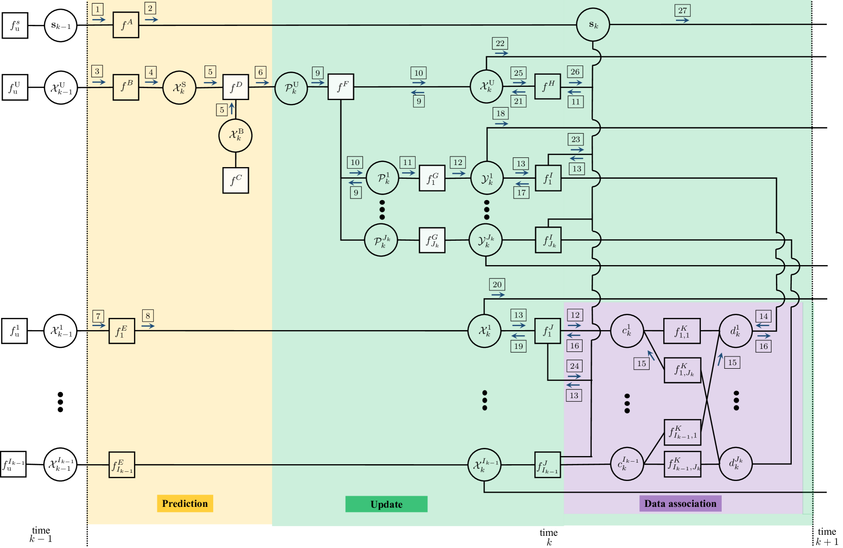
Figure 5: Concatenated factor graph of the joint densities of (40) and (46). The special factors for set densities, discussed in Section III-B, are represented by white squares. The abbreviated notations for the factor nodes are represented by dropping the arguments and $\tilde{(\cdot)}$ on sets, as follows: $f_{\mathsf{u}}^{s}\triangleq\mathtt{b}(\mathbf{s}_{k-1})$, $f_{\mathsf{u}}^{\mathrm{U}}\triangleq\mathtt{b}(\mathcal{X}_{k-1}^{\mathrm{U}})$, $f_{\mathsf{u}}^{i}\triangleq\mathtt{b}(\mathcal{X}_{k-1}^{i})$, $f^{A}\triangleq f^{A}(\mathbf{s}_{k},\mathbf{s}_{k-1})$, $f^{B}\triangleq f^{B}({\mathcal{X}}_{k}^{\mathrm{S}},{\mathcal{X}}_{k-1}^{\mathrm{U}})$, $f^{C}\triangleq f^{C}(\mathcal{X}_{k}^{\mathrm{B}})$, $f^{D}\triangleq f^{D}({\mathcal{X}}_{k}^{\mathrm{S}},{\mathcal{X}}_{k}^{\mathrm{B}},{\mathcal{P}}_{k}^{\mathrm{U}})$, $f_{i}^{E}\triangleq f_{i}^{E}(\mathcal{X}_{k}^{i},\mathcal{X}_{k-1}^{i})$, $f^{F}\triangleq f^{F}({\mathcal{X}}_{k}^{\mathrm{U}},{\mathcal{P}}_{k}^{1},\cdots,{\mathcal{P}}_{k}^{J_{k}})$, $f_{j}^{G}\triangleq f_{j}^{G}({\mathcal{P}}_{k}^{j},{\mathcal{Y}}_{k}^{j})$, $f^{H}\triangleq f^{H}(\mathbf{s}_{k},\mathcal{X}_{k}^{\mathrm{U}})$, $f_{j}^{I}\triangleq f_{j}^{I}(\mathbf{s}_{k},\mathcal{Y}_{k}^{j},d_{k}^{j})$, $f_{i}^{J}\triangleq f_{i}^{J}(\mathbf{s}_{k},\mathcal{X}_{k}^{i},c_{k}^{i})$, and $f_{i,j}^{K}\triangleq f_{i,j}^{K}(c_{k}^{i},d_{k}^{j})$.

IV-B Prediction with Joint Density and Factor Graph

Without loss of generality, we consider two time steps, $k-1$ and $k$, as part of an iterative Bayesian filter. For the factor graph formulation, the joint density for all variables in the prediction is factorized as

$$f(\mathbf{s}_{k-1:k},\tilde{\mathcal{X}}_{k-1}^{\mathrm{U}},\tilde{\mathcal{X}}_{k}^{\mathrm{S}},\tilde{\mathcal{X}}_{k}^{\mathrm{B}},\tilde{\mathcal{P}}_{k}^{\mathrm{U}},\tilde{\mathcal{X}}_{k-1:k}^{1:I_{k-1}})$$

$$\propto f_{\mathtt{u}}(\mathbf{s}_{k-1})f_{\mathtt{u}}^{\mathrm{U}}(\tilde{\mathcal{X}}_{k-1}^{\mathrm{U}})\prod_{i\in\mathcal{I}_{k-1}}f_{\mathtt{u}}^{i}(\tilde{\mathcal{X}}_{k-1}^{i})$$ (40a)

$$\,\,\times f(\mathbf{s}_{k}|\mathbf{s}_{k-1})f^{\mathrm{P}}(\tilde{\mathcal{X}}_{k}^{\mathrm{S}}|\tilde{\mathcal{X}}_{k-1}^{\mathrm{U}})f(\tilde{\mathcal{X}}_{k}^{i}|\tilde{\mathcal{X}}_{k-1}^{i})$$ (40b)

$$\,\,\times f^{\mathrm{U}}(\tilde{\mathcal{X}}_{k}^{\mathrm{B}})\delta_{\tilde{\mathcal{X}}_{k}^{\mathrm{S}}\uplus\tilde{\mathcal{X}}_{k}^{\mathrm{B}}}(\tilde{\mathcal{P}}_{k}^{\mathrm{U}}),$$ (40c)

where $\tilde{\mathcal{X}}_{k-1:k}^{1:I_{k-1}}$ represents the sequence of sets $\tilde{\mathcal{X}}^{i}$ for $i=1,\dots,I_{k-1}$ at time $k$ and $k-1$, and $I_{k-1}$ is the number of Bernoullis at time $k-1$. For completeness, the meaning of each line in (40) is described as follows.

• Posterior at time $k-1$ (40a): This line describes the posterior at time step $k-1$, which is assumed to be $f_{\mathrm{u}}(\mathbf{s}_{k-1},\mathcal{\tilde{X}}_{k-1})=f_{\mathrm{u}}(\mathbf{s}_{k-1})f_{\mathrm{u}}(\mathcal{\tilde{X}}_{k-1})$, where $f_{\mathrm{u}}(\mathbf{s}_{k-1})$ is the sensor state posterior, and $f_{\mathrm{u}}(\tilde{\mathcal{X}}_{k-1}^{\mathrm{U}})$ is the target set posterior. Here $\tilde{\mathcal{X}}_{k-1}$ follows a PMB, endowed with auxiliary variables (see Section II-B3). Due to the auxiliary variables, the PMB posterior at time $k-1$, $f_{\mathrm{u}}(\mathcal{\tilde{X}}_{k-1})$, can be factorized as the product of $f_{\mathrm{u}}(\tilde{\mathcal{X}}_{k-1}^{\mathrm{U}})$ and $f_{\mathrm{u}}(\tilde{\mathcal{X}}_{k-1}^{i})$ for $i\in\mathcal{I}_{k-1}$, where $\mathcal{I}_{k-1}=\{1,\dots,I_{k-1}\}$. Here $\tilde{\mathcal{X}}_{k-1}^{\mathrm{U}}$ is the set of undetected targets (modeled as a PPP), $\tilde{\mathcal{X}}_{k-1}^{i}$ is the set of detected target $i$ (each modeled as a Bernoulli). The subsets $\tilde{\mathcal{X}}_{k-1}^{\mathrm{U}}$ and $\tilde{\mathcal{X}}_{k-1}^{i}$ of $\tilde{\mathcal{X}}_{k-1}^{\mathrm{U}}$ are defined as

  $$\tilde{\mathcal{X}}_{k-1}^{\mathrm{U}} =\{(u,\mathbf{x})\in\tilde{\mathcal{X}}_{k-1}:u=0\},$$ (41)

  $$\tilde{\mathcal{X}}_{k-1}^{i} =\{(u,\mathbf{x})\in\tilde{\mathcal{X}}_{k-1}:u=i\},~{}i\in\mathcal{I}_{k-1}.$$ (42)

  The set densities for targets are given by the form of (13)–(15).

• Transition densities (40b): This line describes the transition densities, where $f(\mathbf{s}_{k}|\mathbf{s}_{k-1})$, $f(\tilde{\mathcal{X}}_{k}^{i}|\tilde{\mathcal{X}}_{k-1}^{i})$, and $f^{\mathrm{P}}(\tilde{\mathcal{X}}_{k}^{\mathrm{S}}|\tilde{\mathcal{X}}_{k-1}^{\mathrm{U}})$ correspond to the sensor state, previously detected targets, and undetected targets. Here $\tilde{\mathcal{X}}_{k}^{\mathrm{S}}$ denotes a surviving set from $\tilde{\mathcal{X}}_{k-1}^{\mathrm{U}}$, modeled as a PPP with auxiliary variable $u=0$. The transition density for Bernoullis with auxiliary variables is

  $$f(\tilde{\mathcal{X}}_{k}|\tilde{\mathcal{Y}}_{k})$$ (43)

  $$=\begin{cases}p_{\mathrm{S}}(\mathbf{y}_{k})f(\mathbf{x}_{k}|\mathbf{y}_{k})\delta_{u_{k}^{\prime}}[u_{k}],&\tilde{\mathcal{X}}_{k}=\{(u_{k},\mathbf{x}_{k})\},\\ &\tilde{\mathcal{Y}_{k}}=\{(u_{k}^{\prime},\mathbf{y}_{k})\}\\ 1-p_{\mathrm{S}}(\mathbf{y}_{k}),&\tilde{\mathcal{X}}_{k}=\emptyset,\\ &\tilde{\mathcal{Y}}_{k}=\{(u_{k}^{\prime},\mathbf{y}_{k})\}\\ 1,&\tilde{\mathcal{X}}_{k}=\emptyset,\tilde{\mathcal{Y}}_{k}=\emptyset\\ 0,&\text{otherwise}\end{cases},$$

  and the transition density for the PPP is

  $$f^{\mathrm{P}}(\tilde{\mathcal{X}}_{k}|\tilde{\mathcal{Y}}_{k})$$ (44)

  $$=\begin{cases}\sum\limits_{\uplus_{i=1}^{n}\tilde{\mathcal{X}}_{k}^{i}=\tilde{\mathcal{X}}_{k}}\prod\limits_{i=1}^{n}f(\tilde{\mathcal{X}}_{k}^{i}|\{\tilde{\mathbf{y}}_{k}^{i}\}),&\tilde{\mathcal{Y}}_{k}=\{\tilde{\mathbf{y}}_{k}^{1},\dots,\tilde{\mathbf{y}}_{k}^{n}\}\\ 1,&\tilde{\mathcal{X}}_{k}=\emptyset,\tilde{\mathcal{Y}}_{k}=\emptyset\\ 0,&\text{otherwise}\end{cases}.$$

  where $f(\tilde{\mathcal{X}}_{k}^{i}|\{\tilde{\mathbf{y}}_{k}^{i}\})$ follows (43) and $\tilde{\mathbf{y}}_{k}^{i}=(0,\mathbf{y}_{k}^{i})$.

• Undetected targets (40c): This last line describes the set-density of newborn targets at time $k$, represented by $f(\tilde{\mathcal{X}}_{k}^{\mathrm{B}})$, where $\tilde{\mathcal{X}}_{k}^{\mathrm{B}}$ denotes a set of newborn targets that follows a PPP, and the set-factor $\delta_{\tilde{\mathcal{X}}_{k}^{\mathrm{S}}\uplus\tilde{\mathcal{X}}_{k}^{\mathrm{B}}}(\tilde{\mathcal{P}}_{k}^{\mathrm{U}})$ merges the set of surviving targets $\tilde{\mathcal{X}}_{k}^{\mathrm{S}}$ and the set of newborn targets $\tilde{\mathcal{X}}_{k}^{\mathrm{B}}$ into the set $\tilde{\mathcal{P}}_{k}^{\mathrm{U}}$ (see also Definition 3). Both $\tilde{\mathcal{X}}_{k}^{\mathrm{B}}$ and $\tilde{\mathcal{P}}_{k}^{\mathrm{U}}$ have auxiliary variable $u=0$.

Using the factorized density in (40), we depict the factor graph for prediction, as shown in Fig. 5 (yellow area). Here we use the following notations for the factor nodes:

$$f^{A}(\mathbf{s}_{k},\mathbf{s}_{k-1})\triangleq f(\mathbf{s}_{k}|\mathbf{s}_{k-1}),$$ (45a)

$$f^{B}(\tilde{\mathcal{X}}_{k}^{\mathrm{S}},\tilde{\mathcal{X}}_{k-1}^{\mathrm{U}})\triangleq f(\tilde{\mathcal{X}}_{k}^{\mathrm{S}}|\tilde{\mathcal{X}}_{k-1}^{\mathrm{U}}),$$ (45b)

$$f^{C}(\tilde{\mathcal{X}}_{k}^{\mathrm{B}})\triangleq f^{\mathrm{U}}(\tilde{\mathcal{X}}_{k}^{\mathrm{B}})$$ (45c)

$$f^{D}(\tilde{\mathcal{X}}_{k}^{\mathrm{S}},\tilde{\mathcal{X}}_{k}^{\mathrm{B}},\tilde{\mathcal{P}}_{k}^{\mathrm{U}})\triangleq\delta_{\tilde{\mathcal{X}}_{k}^{\mathrm{S}}\uplus\tilde{\mathcal{X}}_{k}^{\mathrm{B}}}(\tilde{\mathcal{P}}_{k}^{\mathrm{U}}),$$ (45d)

$$f_{i}^{E}(\tilde{\mathcal{X}}_{k}^{i},\tilde{\mathcal{X}}_{k-1}^{i})\triangleq f(\tilde{\mathcal{X}}_{k}^{i}|\tilde{\mathcal{X}}_{k-1}^{i}).$$ (45e)

We compute the messages on the prediction factor graph in Fig. 5, which has no cycle, by running developed set-type BP. Note that the messages 2, 6, and 8 are equivalent to the marginal densities in prediction of $\mathbf{s}_{k}$, $\tilde{\mathcal{P}}_{k}^{\mathrm{U}}$, and $\tilde{\mathcal{X}}_{k}^{1:I_{k-1}}$, corresponding to prediction of the standard PMB filter [26], represented as $f_{\mathtt{p}}(\mathbf{s}_{k})$, $f_{\mathtt{p}}^{\mathrm{U}}(\tilde{\mathcal{P}}_{k}^{\mathrm{U}})$, and $f_{\mathtt{p}}^{i}(\tilde{\mathcal{X}}_{k}^{i})$ for $i\in\mathcal{I}_{k-1}$.

IV-C Update with Joint Density and its Factor Graph

Without any loss of generality, we consider the update step at time $k$ after the prediction step. The joint density for all variables in the update is

$$f(\mathbf{s}_{k},\tilde{\mathcal{P}}_{k}^{\mathrm{U}},\tilde{\mathcal{P}}_{k}^{1:J_{k}},\tilde{\mathcal{X}}_{k}^{\mathrm{U}},\tilde{\mathcal{Y}}_{k}^{1:J_{k}},\tilde{\mathcal{X}}_{k}^{1:I_{k-1}},\mathbf{c}_{k},\mathbf{d}_{k}|\mathcal{Z}_{k})$$

$$\propto f_{\mathtt{p}}(\mathbf{s}_{k})f_{\mathtt{p}}^{\mathrm{U}}(\tilde{\mathcal{X}}_{k}^{\mathrm{U}})\prod_{i\in\mathcal{I}_{k-1}}f_{\mathtt{p}}^{i}(\tilde{\mathcal{X}}_{k}^{i})$$ (46a)

$$\times\delta_{\tilde{\mathcal{X}}_{k}^{\mathrm{U}}\uplus_{j=1}^{J_{k}}\tilde{\mathcal{P}}_{k}^{j}}(\tilde{\mathcal{P}}_{k}^{\mathrm{U}})\prod_{j\in\mathcal{J}_{k}}\psi(c_{k}^{i},d_{k}^{j})\delta_{\mathtt{h}_{-(I_{k-1}+j)}(\tilde{\mathcal{Y}}_{k}^{j})}(\tilde{\mathcal{P}}_{k}^{j})$$ (46b)

$$\times\tilde{l}(\mathbf{z}_{k}^{j}|\mathbf{s}_{k},\tilde{\mathcal{Y}}_{k}^{j},d_{k}^{j})t(\mathcal{Z}_{k}^{i}|\mathbf{s}_{k},\tilde{\mathcal{X}}_{k}^{i},c_{k}^{i})[1-p_{\mathrm{D}}(\mathbf{s}_{k},\cdot)]^{\tilde{\mathcal{X}}_{k}^{\mathrm{U}}}.$$ (46c)

The proof of (46) is an extension of Appendix E in [28] and [27], found in Appendix E. For completeness, we describe the meaning of each line in (46) as follows.

• Prediction at time $k-1$ (46a): This line describes the predicted densities at time step $k$, discussed at the end of Section IV-B.

• Consistency constraints (46b): This line ensures consistency among the introduced hidden variables. A set of measurements $\mathcal{Z}_{k}$ is provided at time $k$ with index set $\mathcal{J}_{k}=\{1,\dots,J_{k}\}$. We introduce data association variables $\mathbf{c}_{k}\in\mathbb{N}^{I_{k-1}}$, $c_{k}^{i}\in\{0,\dots,J_{k}\}$, and $\mathbf{d}_{k}\in\mathbb{N}^{J_{k-1}}$, $d_{k}^{j}\in\{0,\dots,I_{k-1}\}$, where, in target-oriented data association, $c_{k}^{i}=j$ implies that target $i$ is associated with measurement $j$, and $c_{k}^{i}=0$ implies that target $i$ is not detected. In measurement-oriented data association, $d_{k}^{j}=i>0$ implies that measurement $j$ is associated with target $i$, and $d_{k}^{j}=0$ implies that measurement $j$ originates from either a target that has never been detected or clutter. In particular, we introduced $\Psi(\mathbf{c}_{k},\mathbf{d}_{k})=\prod_{i=1}^{I_{k-1}}\prod_{j=1}^{J_{k}}\psi(c_{k}^{i},d_{k}^{j})$, which ensures mutual consistency between $\mathbf{c}_{k}$ and $\mathbf{d}_{k}$, with $\psi(c_{k}^{i},d_{k}^{j})=0$ when $c_{k}^{i}=j,d_{k}^{j}\neq i~{}\text{or}~{}c_{k}^{i}\neq j,d_{k}^{j}=i$, and 1 otherwise. The factor $\delta_{\tilde{\mathcal{X}}_{k}^{\mathrm{U}}\uplus_{j=1}^{J_{k}}\tilde{\mathcal{P}}_{k}^{j}}(\tilde{\mathcal{P}}_{k}^{\mathrm{U}})$ partitions the set $\tilde{\mathcal{P}}_{k}^{\mathrm{U}}$ into $J_{k}+1$ sets, such that $\tilde{\mathcal{P}}_{k}^{\mathrm{U}}=\tilde{\mathcal{X}}_{k}^{\mathrm{U}}\uplus_{j=1}^{J_{k}}\tilde{\mathcal{P}}_{k}^{j}$, where $\tilde{\mathcal{X}}_{k}^{\mathrm{U}}$ is the set of targets that remain undetected (as indicated by $[1-p_{\mathrm{D}}(\mathbf{s}_{k},\cdot)]^{\tilde{\mathcal{X}}_{k}^{\mathrm{U}}}$ in the likelihood part), and $\tilde{\mathcal{P}}_{k}^{j}$ for $j\in\mathcal{J}_{k}$ represent surviving undetected or newborn targets that are first detected at time $k$. The factor $\delta_{\mathtt{h}_{-(I_{k-1}+j)}(\tilde{\mathcal{Y}}_{k}^{j})}(\tilde{\mathcal{P}}_{k}^{j})$ (see Definition 5) converts the auxiliary variable of $\tilde{\mathcal{P}}_{k}^{j}$ from 0 to $I_{k-1}+j$, turning the set $\tilde{\mathcal{P}}_{k}^{j}$ into a set $\tilde{\mathcal{Y}}_{k}^{j}$ corresponding to a newly detected target (or clutter) arising from measurement $j$. The subsets $\tilde{\mathcal{X}}_{k}^{\mathrm{U}}$, $\tilde{\mathcal{X}}_{k}^{i}$, and $\tilde{\mathcal{Y}}_{k}^{j}$ are defined as

  $$\tilde{\mathcal{X}}_{k}^{\mathrm{U}} =\{(u,\mathbf{x})\in\tilde{\mathcal{X}}_{k}:u=0\},$$ (47)

  $$\tilde{\mathcal{X}}_{k}^{i} =\{(u,\mathbf{x})\in\tilde{\mathcal{X}}_{k}:u=i\},~{}i\in\mathcal{I}_{k-1},$$ (48)

  $$\tilde{\mathcal{Y}}_{k}^{j} =\{(u,\mathbf{x})\in\tilde{\mathcal{X}}_{k}:u=I_{k-1}+j\},~{}j\in\mathcal{J}_{k}.$$ (49)

• Set-likelihoods (46c): This last line describes the likelihood, conditioned on the data association $\mathbf{c}_{k}$ (or equivalently $\mathbf{d}_{k}$). The factor $\tilde{l}(\mathbf{z}_{k}^{j}|\mathbf{s}_{k},\tilde{\mathcal{Y}}_{k}^{j},d_{k}^{j})$ considers potential new targets or clutter, while $t(\mathcal{Z}_{k}^{i}|\mathbf{s}_{k},\tilde{\mathcal{X}}_{k}^{i},c_{k}^{i})$ considers detections and missed detections of the previously detected targets. Both likelihoods are defined as follows. We consider the likelihood when the $j$-th measurement $\mathbf{z}_{k}^{j}$ is associated with a newly detected target or with clutter conditioned on measurement-oriented data association variable $d_{k}^{j}$: $\tilde{l}(\mathbf{z}_{k}^{j}|\mathbf{s}_{k},\tilde{\mathcal{Y}_{k}}^{j},d_{k}^{j})$ is given by

  $$\tilde{l}(\mathbf{z}_{k}^{j}|\mathbf{s}_{k},\tilde{\mathcal{Y}_{k}}^{j},d_{k}^{j})$$ (50)

  $$=\begin{cases}p_{\mathrm{D}}(\mathbf{s}_{k},\mathbf{x}_{k})g(\mathbf{z}_{k}^{j}|\mathbf{s}_{k},\mathbf{x}_{k})\delta_{0}[u_{k}],&\tilde{\mathcal{Y}_{k}}^{j}=\{(u_{k},\mathbf{x}_{k})\},\\ &d_{k}^{j}=0\\ c(\mathbf{z}_{k}),&\tilde{\mathcal{Y}_{k}}^{j}=\emptyset,~{}d_{k}^{j}=0\\ 1,&\tilde{\mathcal{Y}_{k}}^{j}=\emptyset,~{}d_{k}^{j}\neq 0\\ 0,&\mathrm{otherwise}.\end{cases}$$

  Here $p_{\mathrm{D}}(\cdot)$ accounts for the fact that a target may be misdetected, while $c(\mathbf{z}_{k})$ represents the clutter intensity (when a measurement is generated by clutter and not a newly detected target). The function $g(\mathbf{z}_{k}^{j}|\mathbf{s}_{k},\mathbf{x}_{k})$ is a classical likelihood function. Then, the likelihood $t(\mathcal{Z}_{k}^{i}|\mathbf{s}_{k},\tilde{\mathcal{X}}_{k}^{i},c_{k}^{i})$ considers the case when a set $\mathcal{Z}_{k}^{i}$ is associated to the $i$-th previously detected target conditioned on target-oriented data association variable $c_{k}^{i}$:

  $$t(\mathcal{Z}_{k}^{i}|\mathbf{s}_{k},\tilde{\mathcal{X}}_{k}^{i},c_{k}^{i})$$ (51)

  $$=\begin{cases}p_{\mathrm{D}}(\mathbf{s}_{k},\mathbf{x}_{k}^{i})g(\mathbf{z}_{k}^{j}|\mathbf{s}_{k},\mathbf{x}_{k}^{i})\delta_{i}[u_{k}],&\mathcal{Z}_{k}^{i}=\{\mathbf{z}_{k}^{j}\},~{}c_{k}^{i}=j,\\ &\tilde{\mathcal{X}}_{k}^{i}=\{(u_{k},\mathbf{x}_{k}^{i})\}\\ (1-\mathtt{p}_{\mathrm{D}}(\mathbf{s}_{k},\mathbf{x}_{k}^{i}))\delta_{i}[u_{k}],&\mathcal{Z}_{k}^{i}=\emptyset,~{}c_{k}^{i}=0,\\ &\tilde{\mathcal{X}}_{k}^{i}=\{(u_{k},\mathbf{x}_{k}^{i})\}\\ 1,&\mathcal{Z}_{k}^{i}=\emptyset,~{}c_{k}^{i}=0,\\ &\tilde{\mathcal{X}}_{k}^{i}=\emptyset\\ 0,&\mathrm{otherwise}.\end{cases}$$

  The factor $[1-p_{\mathrm{D}}(\mathbf{s}_{k},\cdot)]^{\tilde{\mathcal{X}}_{k}^{\mathrm{U}}}$ describes the set of targets that remain undetected.

Using the factorized density in (46), we depict the factor graph for update, as shown in Fig. 5 (green area). Here we use the following notations for the factor nodes:

$$f^{F}(\tilde{\mathcal{X}}_{k}^{\mathrm{U}},\tilde{\mathcal{P}}_{k}^{1},\cdots,\tilde{\mathcal{P}}_{k}^{J_{k}})\triangleq\delta_{\tilde{\mathcal{X}}_{k}^{\mathrm{U}}\uplus_{j=1}^{J_{k}}\tilde{\mathcal{P}}_{k}^{j}}(\tilde{\mathcal{P}}_{k}^{\mathrm{U}}),$$ (52a)

$$f_{j}^{G}(\tilde{\mathcal{P}}_{k}^{j},\tilde{\mathcal{Y}}_{k}^{j})\triangleq\delta_{\mathtt{h}_{-(I_{k-1}+j)}(\tilde{\mathcal{Y}}_{k}^{j})}(\tilde{\mathcal{P}}_{k}^{j}),$$ (52b)

$$f^{H}(\mathbf{s}_{k},\tilde{\mathcal{X}}_{k}^{\mathrm{U}})\triangleq[1-p_{\mathrm{D}}(\mathbf{s}_{k},\cdot)]^{\tilde{\mathcal{X}}_{k}^{\mathrm{U}}},$$ (52c)

$$f_{j}^{I}(\mathbf{s}_{k},\tilde{\mathcal{Y}}_{k}^{j},d_{k}^{j})\triangleq\tilde{l}(\mathbf{z}_{k}^{j}|\mathbf{s}_{k},\tilde{\mathcal{Y}}_{k}^{j},d_{k}^{j}),$$ (52d)

$$f_{i}^{J}(\mathbf{s}_{k},\tilde{\mathcal{X}}_{k}^{i},c_{k}^{i})\triangleq t(\mathcal{Z}_{k}^{i}|\mathbf{s}_{k},\tilde{\mathcal{X}}_{k}^{i},c_{k}^{i}),$$ (52e)

$$f_{i,j}^{K}(c_{k}^{i},d_{k}^{j})\triangleq\psi(c_{k}^{i},d_{k}^{j}).$$ (52f)

We compute the messages and beliefs on the update factor graph in Fig. 5 by running developed set-type BP, detailed in Appendix F of the supplementary material. As a final result, the message 27 represents the posterior of the sensor state at the end of time step $k$, 22 represents the posterior PPP of undetected targets, 18 represents the posteriors of the Bernoullis of each newly detected target, and 20 represents the posteriors of the Bernoullis of each previously detected target. These posteriors will be used when creating the factor graph connecting time step $k$ with time step $k+1$. Note that the number of detected targets grows over time.

IV-D Connecting the Factor Graphs in Prediction and Update

So far, we have discussed the prediction and update factor graphs independently. We now proceed to explain how these factor graphs are connected. The factor graph in the prediction (see, yellow part in Fig. 5) includes variable nodes $\mathbf{s}_{k},\tilde{\mathcal{P}}_{k}^{\mathrm{U}},\tilde{\mathcal{X}}_{k}^{1},\dots,\tilde{\mathcal{X}}_{k}^{I_{k-1}}$ while the factor graph in the update (see, green and purple parts in Fig. 5) contains variables $\mathbf{s}_{k},\tilde{\mathcal{X}}_{k}^{\mathrm{U}},\tilde{\mathcal{P}}_{k}^{1},\dots,\tilde{\mathcal{P}}_{k}^{J_{k}},\tilde{\mathcal{X}}_{k}^{1},\dots,\tilde{\mathcal{X}}_{k}^{I_{k-1}}$. We note that the variables $\mathbf{s}_{k},\tilde{\mathcal{X}}_{k}^{1},\dots,\tilde{\mathcal{X}}_{k}^{I_{k-1}}$ are the same. To connect the other variable nodes in the prediction and update factor graphs, we can use a merging and partitioning factor (see, Definition 3) as well as a conversion factor for auxiliary variables (see, Definition 5) for newly detected Bernoullis. That is, we first adopt the factor $f^{F}(\tilde{\mathcal{P}}_{k}^{\mathrm{U}},\tilde{\mathcal{X}}_{k}^{\mathrm{U}},\tilde{\mathcal{P}}_{k}^{1},\dots,\tilde{\mathcal{P}}_{k}^{J_{k}})$, which partitions the set $\tilde{\mathcal{P}}_{k}^{\mathrm{U}}$ into subsets $\tilde{\mathcal{X}}_{k}^{\mathrm{U}},\tilde{\mathcal{Y}}_{k}^{1},\dots,\tilde{\mathcal{Y}}_{k}^{J_{k}}$ (all with auxiliary variable 0). Then, to each of the newly detected Bernoullis, we apply the conversion factor for auxiliary variables $f_{j}^{G}(\tilde{\mathcal{P}}_{k}^{j},\tilde{\mathcal{Y}}_{k}^{j})$. Considering the set-variables that are linked to the set-factors $f^{F}(\cdot)$ and $f_{j}^{G}(\cdot)$, see Fig. 5, we know that the set-variable $\tilde{\mathcal{Y}}_{k}^{j}$ and ${\mathcal{X}}_{k}^{\mathrm{U}}$ follow a Poisson process with $u=I_{k-1}+j$ and $u=0$, respectively. Finally, the factor graphs for prediction and update are connected by the factors ($f^{A}(\cdot)$, $f^{D}(\cdot)$, and $f_{i}^{E}(\cdot)$) and their linked variables.

Remark 2 (Factor Graphs for Smoothing at the Previous Time Step).

Fig. 5 shows the concatenation of factor graphs for the prediction and update steps at time $k-1$ and $k$. It is possible to derive a joint prediction and update factor graph (instead of its concatenation). This factor graph would require the use of PMBs for sets of trajectories between time $k-1$ and $k$ [41, 42]. Furthermore, this factor graph would enable us to infer the state at time $k-1$ of a Bernoulli created at time $k$, via smoothing.

Remark 3 (Special Cases and Generalizations).

The factorization ((40) and (46)) and the corresponding factor graph in Fig. 5 can be specialized and generalized to cover a variety of applications. Some special cases include:

• Mapping and SLAM are obtained when the targets have no mobility, which is obtained when the transition density is $f(\mathbf{x}_{k}|\mathbf{x}_{k-1})=\delta(\mathbf{x}_{k}-\mathbf{x}_{k-1})$.

• Mapping and MTT are obtained when then sensor state is known at all times, so that $f_{\mathtt{u}}(\mathbf{s}_{k-1})$ and $f(\mathbf{s}_{k}|\mathbf{s}_{k-1})$ are removed and $\bm{s}_{k-1}$ and $\bm{s}_{k}$ no longer explicitly appear as vertices in the factor graph (instead they are absorbed as parameters in the likelihood functions).

Remark 4 (Set-Type BP MB Filter).

To obtain a set-type BP MB filter (whether labeled or not), we use the same modeling assumptions as in the set-type BP PMB filter except that the birth model is MB instead of Poisson. Then, we set the intensity of PPP to zero and add the Bernoulli components of the birth process in the prediction step [43]. The corresponding factor graph is equivalent to the one in Fig. 5 but removing all the PPP variables ($\mathcal{X}_{k-1}^{\mathrm{U}},\mathcal{X}_{k}^{\mathrm{S}},\mathcal{X}_{k}^{\mathrm{B}},\mathcal{P}_{k}^{\mathrm{U}},\mathcal{P}_{k}^{1},\dots,\mathcal{P}_{k}^{J_{k}},\mathcal{X}_{k}^{\mathrm{U}}$), their connected factors ($f_{\mathsf{u}}^{\mathrm{U}},f^{B},f^{C},f^{D},f^{F},f_{1}^{G},\dots,f_{J_{k}}^{G}$), and newly detected targets ($\mathcal{Y}_{k}^{1},\dots,\mathcal{Y}_{k}^{J_{k}}$), and also adding the new birth Bernoulli variables and factors in the prediction step.

Remark 5 (On the Use of Set-Type BP with Other RFS Filters).

It should be noted that set-type BP can be used to derive RFS filters based on computing marginal distributions for targets, such as PMB and MB filters. It is not suitable to derive PHD and CPHD filters as these filters do not calculate marginals but approximate the posterior as a PPP or as an independent and identically distributed cluster process [22]. Set-type BP is also not suitable for implementing filters based on conjugate priors such as PMBM and $\delta$-GLMB filters.

IV-E Approximate KLD Minimization of Set-Type BP PMB for SLAM

Assuming that the prior is a PMB, the prediction of the set-type BP is represented in closed-form. As a direct application of the PMBM update [28, Sec. IV-B], the updated density is $\tilde{f}_{\mathsf{u}}^{\mathrm{PMBM}}(\tilde{\mathcal{X}}_{k}|\mathbf{s}_{k})f_{\mathsf{u}}(\mathbf{s}_{k})$, where $\tilde{f}_{\mathsf{u}}^{\mathrm{PMBM}}(\tilde{\mathcal{X}}_{k}|\mathbf{s}_{k})$ corresponds to the PMBM with the auxiliary variables [42, Sec. III-A], given the sensor state $\mathbf{s}_{k}$, where $\tilde{\mathcal{X}}_{k}=\tilde{\mathcal{X}}_{k}^{\mathrm{U}}\uplus\tilde{\mathcal{X}}_{k}^{1:I_{k-1}}\uplus\tilde{\mathcal{Y}}_{k}^{1:J_{k}}$ (see, (46)).

Lemma 1.

The marginals of $\mathbf{s}_{k}$, $\tilde{\mathcal{X}}_{k}^{\mathrm{U}}$, $\tilde{\mathcal{X}}_{k}^{i}$, $\tilde{\mathcal{Y}}_{k}^{j}$ of (46) represent a PMB that is an optimal approximation of the corresponding PMBM posterior in the sense that it minimizes the Kullback-Leibler divergence (KLD) $D(\tilde{f}_{\mathsf{u}}^{\mathrm{PMBM}}(\tilde{\mathcal{X}}_{k}|\mathbf{s}_{k})f_{\mathsf{u}}(\mathbf{s}_{k})||\tilde{q}_{\mathtt{u}}^{\mathrm{PMB}}(\tilde{\mathcal{X}})q_{\mathtt{u}}(\mathbf{s}_{k}))$. The marginal densities of $\mathbf{s}_{k}$, $\tilde{\mathcal{X}}_{k}^{\mathrm{U}}$, $\tilde{\mathcal{X}}_{k}^{i}$, $\tilde{\mathcal{Y}}_{k}^{j}$ are given by

$$\tilde{q}_{\mathtt{u}}^{\mathrm{PMB}}(\tilde{\mathcal{X}}) =\tilde{q}_{\mathtt{u}}^{\mathrm{U}}(\tilde{\mathcal{X}}^{\mathrm{U}})\prod_{i=1}^{n}\tilde{q}_{\mathtt{u}}^{i}(\tilde{\mathcal{X}}^{i}),$$ (53)

$$q_{\mathtt{u}}(\mathbf{s}_{k}) =f_{\mathtt{u}}(\mathbf{s}_{k}),$$ (54)

$$q_{\mathtt{u}}(\tilde{\mathcal{X}}_{k}^{\mathrm{U}}) =\int f_{\mathtt{u}}(\tilde{\mathcal{X}}_{k}^{\mathrm{U}}|\mathbf{s}_{k})f_{\mathtt{u}}(\mathbf{s}_{k})\mathrm{d}\mathbf{s}_{k},$$ (55)

$$q_{\mathtt{u}}(\tilde{\mathcal{X}}_{k}^{i}) =\int f_{\mathtt{u}}(\tilde{\mathcal{X}}_{k}^{i}|\mathbf{s}_{k})f_{\mathtt{u}}(\mathbf{s}_{k})\mathrm{d}\mathbf{s}_{k},$$ (56)

$$q_{\mathtt{u}}(\tilde{\mathcal{Y}}_{k}^{j}) =\int f_{\mathtt{u}}(\tilde{\mathcal{Y}}_{k}^{j}|\mathbf{s}_{k})f_{\mathtt{u}}(\mathbf{s}_{k})\mathrm{d}\mathbf{s}_{k}.$$ (57)

Then, upon convergence, the set-type BP applied to (46) approximates these marginal densities by producing the interior points of the constrained Bethe free energy on the factor graph, see Theorem 1.

Proof.

The proof of the KLD minimization is an extension of Proposition 1 of [41], showing the optimality of the solution. The Bethe free minimization is a result of Theorem 1. ∎

IV-F Exploring the Relationships: Set-Type and Vector-Type BP PMB-SLAM Implementations

We now reveal connections between the proposed set-type BP filter to the vector-type BP filters [12, 13]. The connections between them are described from the following viewpoints: (i) models for problem formulation; (ii) messages and beliefs on the factor graph. We note that the connection between vector-type and RFS-based method was partially discussed from the perspective of the expression of target densities and data association in [9, Sec. XIII-A] and [28, Sec. IV-E].

IV-F1 Models

Set-type BP and vector-type BP differ in several ways in the modeling of the problem:

• Undetected targets: In vector-type BP, undetected targets are not explicitly formulated as the variables of the joint density [12, eq. (16)], and thus ad-hoc modifications with the auxiliary PHD are adopted to address undetected targets, outside of the vector-type BP factor graph. On the other hand, undetected targets are explicitly included as one of variables of the joint PMBM density (46) in proposed set-type BP.

• Detected targets: Both BP variants consider an unknown number of targets as well as unknown target states. To account for the existence probabilities in vector-type BP, each target state vector is augmented vector with a binary existence variable $\epsilon$, leading to $\mathbf{y}^{i}=[(\mathbf{x}^{i})^{\top},\epsilon^{i}]^{\top}$, indicating a single target with the density $f(\mathbf{x}^{i},\epsilon^{i})$. It follows that the densities of detected targets in vector-type BP are equivalent to the Bernoulli densities in RFS methods, with $f(\mathbf{x},\epsilon=1)=f(\mathcal{X}=\mathbf{x})=rf(\mathbf{x})$ and $f(\mathbf{x},\epsilon=0)=f(\mathcal{X}=\emptyset)=1-r$.

IV-F2 Messages and Beliefs

The two BP variants also have commonalities and differences in terms of the messages and beliefs on the factor graph:

• Predicted messages: In both BP variants, the messages from the sensor transition factor to the sensor state are identical. The messages from the target transition factor to the previously detected target are also identical since the target density in vector-type BP is identical to the Bernoulli density. The messages for undetected targets can be explicitly computed using the factor graph for the set-type BP approach. Undetected targets in vector-type BP are dealt with via the prediction step of the PHD filter, outside of the factor graph, leading to the same results.

• Data association: In both BP variants, the BP-based data association approach [26] is adopted. Due to the same messages for the sensor state and previously detected targets in the prediction step, the messages from the likelihood functions of previously detected targets to the target-oriented data association variables are identical. Even though the messages for undetected targets are not explicitly represented in the factor graph of vector-type BP, due to the external addition of the auxiliary PHD, the messages from the likelihood functions of undetected targets to the measurement-oriented association variables are identical to set-type BP. It follows that the input messages to the association variables are identical, and thus the output messages after the data association step are also identical.

• Beliefs: Due to the fact that in both BP variants, the messages from the sensor state, previously detected targets, and target-oriented data association variables to likelihood functions for previously detected targets are identical. Therefore, the beliefs at previously detected targets are the same. As we discussed above, even though the messages for undetected targets are not explicitly represented in the factor graph of vector-type BP, the beliefs at newly detected targets with the ad-hoc process of the auxiliary PHD in vector-type BP are identical to the set-type BP. In vector-type BP, the messages for undetected targets that remain undetected are not explicitly expressed. Again this can be addressed if the missed detections are considered in the ad-hoc process with the auxiliary PHD, so that the messages are identical to set-type BP. For the sensor state update, the messages for newly detected targets and undetected targets that remain undetected again are not addressed in vector-type BP. This is because the corresponding factor graph and messages cannot be explicitly formulated. However, the messages from undetected targets can be explicitly derived in the proposed method due to developed set-type BP, running on the formulated factor graph (see, Fig. 5).

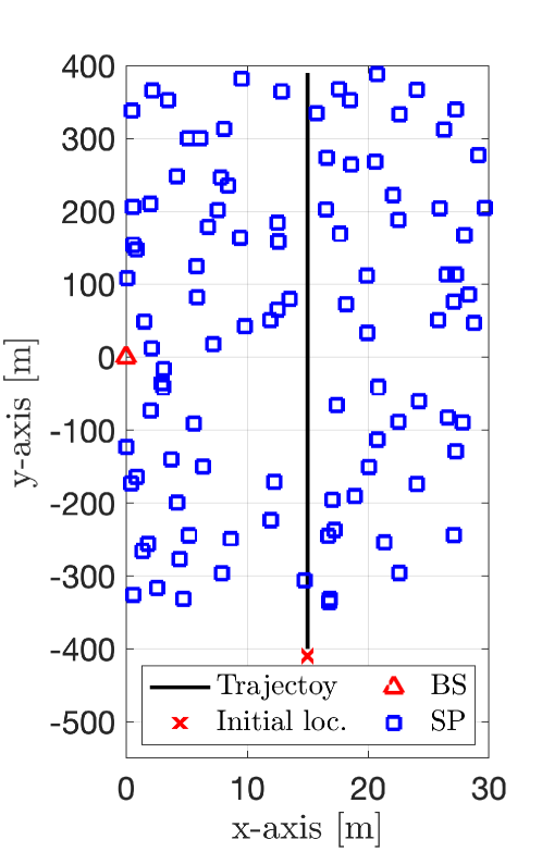
Figure 6: Bistatic radio SLAM scenario, where the SPs are uniformly distributed. A single BS transmits the signal, and the sensor receives the two types of measurements: BS-sensor; and BS-SPs-sensor.

V Numerical Results

In this section, we analyze the proposed set-type BP PMB-SLAM and BP MB-SLAM filters in comparison with BP-SLAM [12, 13]. We introduce the simulation setup for evaluating the SLAM filters, and subsequently the results are discussed.

(a)

(b)

Figure 7: Uninformative birth case. Comparison of the proposed set-type BP PMB-SLAM and vector-type BP-SLAM [12, 13]: (a) RMSEs of sensor localization and (b) GOSPA errors of landmark mapping.

(a)

(b)

Figure 8: Informative birth case. Comparison of the proposed set-type BP PMB-SLAM and vector-type BP-SLAM [12, 13]: (a) RMSEs of sensor localization and (b) GOSPA errors of landmark mapping. The performance of set-type BP MB-SLAM is identical to set-type BP PMB-SLAM, and the plot is omitted.

V-A Simulation Setup

V-A1 Environments

We consider a bistatic radio SLAM scenario, where a single base station (BS) transmits the pilot signals, and scattering points (i.e., landmarks) are uniformly distributed, as shown in Fig. 6. A single sensor can receive two types of measurements: one from BS-sensor path; and others from BS-SPs-sensor paths. We denote the locations of the BS and SP $j$ by $\mathbf{x}_{\mathrm{BS}}$ and $\mathbf{x}_{\text{SP}}^{j}$. The sensor state at time $k$ is denoted by $\mathbf{s}_{k}=[\mathbf{x}_{k,s}^{\top},\dot{\mathbf{x}}_{k,s}^{\top}]^{\top}$, where $\mathbf{x}_{k,s}=[x_{k,s},y_{k,s}]^{\top}$ denotes the location, and $\dot{\mathbf{x}}_{k,s}=[\dot{x}_{k,s},\dot{y}_{k,s}]^{\top}$ denotes the velocity.

V-A2 Dynamics

For the sensor dynamics, we adopt constant-velocity motion model [44, Sec. 6.3.2] with the known transition density $f(\mathbf{s}_{k}|\mathbf{s}_{k-1})$, and the sensor state evolution follows

$$\mathbf{s}_{k}=\mathbf{F}\mathbf{s}_{k-1}+\mathbf{B}\mathbf{q}_{k},$$ (58)

$\mathbf{F}$ and $\mathbf{B}$ are defined as [44, Sec. 6.3.2]

$$\mathbf{F}=\begin{bmatrix}\mathbf{I}_{2\times 2}&\Delta t\mathbf{I}_{2\times 2}\\ \mathbf{0}_{2\times 2}&\mathbf{I}_{2\times 2}\end{bmatrix}, \mathbf{B}=\begin{bmatrix}0.5\Delta t^{2}\mathbf{I}_{2\times 2}\\ \Delta t\mathbf{I}_{2\times 2}\end{bmatrix}.$$ (59)

Here $\Delta t$ is the sampling time, and $\mathbf{q}_{k}$ is the driving process that follows zero-mean Gaussian distribution with the covariance matrix $\sigma_{w}^{2}\mathbf{I}_{2\times 2}$, where $\sigma_{w}$ is the standard deviation, and $\mathbf{I}_{2\times 2}$ is the 2 by 2 identity matrix.

V-A3 Measurements

The sensor obtains the measurement set $\mathcal{Z}_{k}=\{\mathbf{z}_{k}^{0},\mathbf{z}_{k}^{1},\dots,\mathbf{z}_{k}^{J_{k}}\}$, where $\mathbf{z}_{k}^{0}$ and $\mathbf{z}_{k}^{j}$ for $j>0$ are the measurements corresponding to the BS and different SPs, respectively. Let $\mathbf{t}_{k}^{j}=[({\mathbf{x}_{\text{SP}}^{j}})^{\top},\mathbf{x}_{k,s}^{\top}]^{\top}$ be the augmented vector of SP location $\mathbf{x}_{\text{SP}}^{j}$ and the sensor location $\mathbf{x}_{k,s}$. With the known BS location, the measurements $\mathbf{z}_{k}^{0}$ and $\mathbf{z}_{k}^{j}$ for $j>0$ are modeled as

$$\mathbf{z}_{k}^{0} =\mathbf{x}_{k,s}+\mathbf{r}_{k},$$ (60)

$$\mathbf{z}_{k}^{j} =\mathbf{H}\mathbf{t}_{k}^{j}+\mathbf{r}_{k}.$$ (61)

Here $\mathbf{H}=[\mathbf{I}_{2\times 2},-\mathbf{I}_{2\times 2}]$, and $\mathbf{r}_{k}$ is the measurement noise that follows zero-mean Gaussian distribution with the covariance $\sigma_{r}^{2}\mathbf{I}_{2\times 2}$, where $\sigma_{r}$ is the standard deviation. We regard the false alarms and shortly visible SPs as clutter, modeled as $\mathbf{z}_{k}^{\mathrm{C}}\in\mathcal{Z}_{k}$.

V-A4 Scenarios and Parameters

We investigate the performance gain of the proposed set-type BP MB and PMB-SLAM filters, compared to the vector-type BP-SLAM method [12, 13]. We consider $K$ time steps with two scenarios as follows: one with an uninformative birth model, and the other with an informative birth model in modeling of undetected landmarks. In realistic environments, the uninformative birth model represents cases where we lack prior map knowledge, whereas the informative birth models the assumption that we have a previously available map. In both birth models, the landmarks are observable starting from $k=5$, and additional landmarks can be observable at each subsequent time step. For sensor localization in both scenarios, multipath is employed from $k=5$, whereas for $k<5$ the measurement for BS-sensor path is exploited.

For set-type BP PMB-SLAM, undetected landmarks and the birth are modeled by the PPP process, implemented by the intensity functions. The intensities for undetected targets and the birth are represented by $\lambda(\mathbf{x})=\sum_{q}\eta^{q}\mathsf{N}(\mathbf{x};\mathbf{x}^{q},\mathbf{U}^{q})$ and $\lambda^{\mathrm{B}}(\mathbf{x})=\sum_{q}\eta^{\mathrm{B},q}\mathsf{N}(\mathbf{x};\mathbf{x}^{\mathrm{B},q},\mathbf{U}^{\mathrm{B},q})$, where $\mathsf{N}(\mathbf{x};\mathbf{x},\mathbf{U})$ is the Gaussian density, and $\eta$ is the Gaussian weight. For set-type BP MB-SLAM, the birth is modeled by the MB process. The MB birth density is the form of (11), where the $q$-th Bernoulli has an existence probability $r^{\text{B},q}$ and Gaussian density $\mathsf{N}(\mathbf{x};\mathbf{x}^{\text{B},q},\mathbf{U}^{\text{B},q})$. For both birth cases, we set $\mathbf{x}^{\text{B},q}\sim\mathsf{N}(\mathbf{x};\mathbf{x}_{\text{SP}},\mathbf{U}^{\text{B},q})$; for the informative birth case, $\eta^{\text{B},q}=1$ and $\mathbf{U}^{\text{B},q}=0.01\mathbf{I}_{2\times 2}$; and for the uninformative birth case, $\eta^{\text{B},q}=10^{-3}$ and $\mathbf{U}^{\text{B},q}=10^{6}\times\mathbf{I}_{2\times 2}$. Using the Kalman filter [46], we implement the messages and beliefs corresponding to landmarks and data associations. The belief of the sensor state of 27 is intractable by the Kalman filter, and thus implemented by the particle filter [47, 4] with $N_{\mathrm{P}}$ samples. After the belief computation at each time step, we declare that a landmark is detected when $r_{k|k}^{i}>\Gamma_{\mathrm{D}}$. The previously detected landmarks with $r_{k|k}^{i}<\Gamma_{\mathrm{Ber}}$ for $i=1,\dots,I_{k-1}+J_{k}$ are removed, and the Gaussians in the PPP with $\eta_{k|k}^{q}<\Gamma_{\mathrm{Poi}}$ are eliminated.

We set the prior density of the sensor state to $f(\mathbf{s}_{0})=\mathsf{N}(\mathbf{s}_{0};\mathbf{s}_{0|0},\mathbf{P}_{0|0})$, where $\mathbf{s}_{0|0}$ is sampled from $\mathsf{N}(\bar{\mathbf{s}}_{0},\mathbf{P}_{0|0})$ for each simulation run. Here $\bar{\mathbf{s}}_{0}=[15,-420,0,20]^{\top}$ is the ground truth of the initial sensor state, with the units of m, m, m/s, and m/s, and $\mathbf{P}_{0|0}=\mathrm{blkdiag}[0.5\mathbf{I}_{2\times 2},0.005\mathbf{I}_{2\times 2}]$, and the units of the diagonal term of $\mathbf{P}$ are m², m², m²/s², and m²/s². The BS location is set to $\mathbf{x}_{\mathrm{BS}}=[0,0]^{\top}$, and 150 SPs are uniformly distributed in $[30,70]$ m $\times[55,805]$ m. The radius of the field-of-view of the sensor is 20 m, and the landmarks begin to be observable at time $k=5$. To investigate the influence of newly detected landmarks on sensor state updates, we set up the map environment so that an average of two landmarks are newly detected at every single time step. The number of clutter measurements, which are observed by the sensor, is modeled by the Poisson distribution with mean $\mu_{\mathrm{c}}$ [41], and the clutter intensity is denoted by $c(\mathbf{z})$. For both informative and uninformative births, $\mu_{\mathrm{c}}=1$, $c(\mathbf{z})=1.6\cdot 10^{-4}$ in the area of interest. The rest of the simulation parameters are set as follows: $K=80$; $\sigma_{w}=0.1$ m/s²; $\sigma_{r}=0.707$ m; $\Delta t=0.5$ s; $N_{p}=10^{4}$, $\Gamma_{\mathrm{D}}=0.4$; $\Gamma_{\mathrm{Ber}}=10^{-5}$; $\Gamma_{\mathrm{Poi}}=5\cdot 10^{-10}$. For simplicity, we set the detection probability and survival probability to constant values [12, 26]: $p_{\mathrm{D}}(\cdot)=p_{\mathrm{D}}=0.95$ and $p_{\mathrm{S}}(\cdot)=p_{\mathrm{S}}=0.99$. The simulation results are averaged over 500 Monte Carlo trials.

The performance of sensor localization and landmark mapping are evaluated by root mean square error (RMSE) and generalized optimal subpattern assignment (GOSPA) [48, eq. (1)] with parameters $\mathrm{G}_{p}=1$, $\mathrm{G}_{c}=2$, and $\mathrm{G}_{\alpha}=2$, respectively.

V-B Results and Discussions

V-B1 Uninformative Birth

Fig. 7 shows the SLAM performance against time, under the scenario that the PPP for undetected landmarks and birth in set-type BP PMB and the MB for birth in set-type BP MB are uninformative. During $K=80$, the SLAM performance of the set-type BP PMB filter is identical to that of the vector-type BP filter even though the messages 23 are employed for sensor belief computation. This happens because the messages 23 corresponding to newly detected landmarks or clutter are not as informative as the messages 20 corresponding to previously detected landmarks. The mapping performance of the set-type BP MB filter is inferior to the other two filters. This is because the MB birth model is limited in the number of Bernoulli sets, where each is available for modeling a single landmark, whereas the set that follows PPP captures multiple landmarks.

V-B2 Informative Birth

Fig. 8 shows the SLAM performance against time, under the scenario that the PPP for undetected landmarks and birth in set-type BP PMB and MB birth in set-type BP MB are informative. When using the informative PPP, we achieve the performance improvement in set-type BP PMB-SLAM compared to that of vector-type BP-SLAM. This is because new landmarks appear and the PPP for undetected landmarks is informative. The sensor localization gap is clearly visible, and the landmarks are determined, starting from $k=5$ since the landmarks begin to be observable from $k=5$. The gap of GOSPAs increases over time steps because there exist newly detected landmarks at every time step. We obtain that the performance of set-type BP MB-SLAM is identical to that of BP PMB-SLAM, and thus the results are omitted. This is because the clutter part of the messages 23 is much smaller than the newly detected landmark part, and the implementation of MB birth for set-type BP MB-SLAM is equivalent to that of set-type BP PMB-SLAM, under the informative birth case.

Tables I and II present the RMSEs of sensor localization and GOSPA errors of landmark mapping respectively, with the different clutter setup: $\mu_{c}=1$ with $c(\mathbf{z})=1.6\cdot 10^{-4}$, $\mu_{c}=5$ with $c(\mathbf{z})=8\cdot 10^{-4}$, and $\mu_{c}=10$ with $c(\mathbf{z})=1.6\cdot 10^{-3}$. The results are averaged over all Monte Carlo simulation runs during the steady-state operation after $k>40$. Tables I and II show the performance of both methods deteriorates progressively as the clutter Poisson mean $\mu_{c}$ increases ($\mu_{c}=1,\mu_{c}=5,\mu_{c}=10$). The performance gap between set-type BP PMB-SLAM and vector-type BP-SLAM arises from the usage of newly detected targets in sensor state updates, which could be computed thanks to the proposed set-type BP framework.

TABLE I: Informative birth case: RMSEs of Sensor Localization

2	$\mu_{c}=1$	$\mu_{c}=5$	$\mu_{c}=10$
Vector-type BP [12]	0.1651	0.1881	0.2014
Set-type BP (PMB)	0.1306	0.1334	0.1401
2

TABLE II: Informative birth case: GOSPA Errors of Landmark Mapping

2	$\mu_{c}=1$	$\mu_{c}=5$	$\mu_{c}=10$
Vector-type BP [12]	638.48	979.74	1162.34
Set-type BP (PMB)	636.42	977.31	1160.52
2

VI Conclusions

In this paper, we have developed the general framework of set-type BP, which can serve as a fundamental tool for computing either the marginal (or its approximate density) of an RFS. From the framework, we derived the PMB and MB filters with the developed set-type BP, applicable to the related problems of mapping, MTT, SLAM, and SLAT. Under the densities that follow the Bernoulli process, we demonstrated that vector-type BP is the special case of set-type BP. To handle the unknown set cardinality in the factor graph, we developed the set-factor nodes for set partitioning, set merging, and shifting set auxiliary variables. We applied the proposed set-type BP to PMB-SLAM filter and explored the relations between the set-type BP PMB and vector-type BP-SLAM [12, 13] filters. Our results demonstrated that the proposed set-type BP-SLAM filter outperforms the vector-type BP, under the informative PPP for undetected landmarks, and equivalent for the uninformative PPP. Set-type BP can thus also serve as a way to improve vector-type BP, through new heuristics, to match the performance and operation of set-type BP.

Possible extensions include smoothing (obtained by computing messages backward in time), cooperative processing (obtained by linking the factor graphs related to two different sensors), and positioning (by adding factors related to fixed anchors in the environment). Furthermore, applications of the set-type BP framework to other families of RFS filters, along with its BP counterpart [49], deserve further study.

Appendix A Proof of Theorem 1

We prove Theorem 1 in a similar fashion as in the vector-type BP [3, Theorem 2].

Proof.

Using the set beliefs of (20) and (21), we introduce the Bethe free energy [3]: $F_{\mathrm{Bethe}}=U_{\mathrm{Bethe}}-H_{\mathrm{Bethe}}$, where $U_{\mathrm{Bethe}}$ is the Bethe average energy, given by

$$U_{\mathrm{Bethe}}=-\sum_{a}\int\mathtt{b}(\underline{\mathcal{X}}^{a})\ln f_{a}(\underline{\mathcal{X}}^{a})\delta\underline{\mathcal{X}}^{a},$$ (62)

and $H_{\mathrm{Bethe}}$ is the Bethe entropy, given by

$$H_{\mathrm{Bethe}}= \,-\sum_{a}\int\mathtt{b}(\underline{\mathcal{X}}^{a})\ln\mathtt{b}(\underline{\mathcal{X}}^{a})\delta\underline{\mathcal{X}}^{a}$$

$$+\sum_{i}(\lvert\mathcal{M}(i)\rvert-1)\int\mathtt{b}(\mathcal{X}^{i})\ln\mathtt{b}(\mathcal{X}^{i})\delta\mathcal{X}^{i}.$$ (63)

The constraints of the Bethe free energy, the average energy, and the entropy are all functions of set-beliefs. They are introduced as follows. The normalization constraints are $\int\mathtt{b}(\mathcal{X}^{i})\delta\mathcal{X}^{i}=1$ for all set-variable $i$, $\int\mathtt{b}(\underline{\mathcal{X}}^{a})\delta\underline{\mathcal{X}}^{a}=1$ for all set-factor $a$ with $\lvert\mathcal{M}(i)\rvert\geq 2$. The marginalization constraints are $\int\mathtt{b}(\underline{\mathcal{X}}^{a})\delta\mathcal{X}^{\sim i}=\mathtt{b}(\mathcal{X}^{i})$ such that $i\in\mathcal{N}(a)$. The inequality constraints are $0\leq\mathtt{b}(\underline{\mathcal{X}}^{a})\leq 1$ for all set-factor $a$ and $0\leq\mathtt{b}(\mathcal{X}^{i})\leq 1$ for all set-variable $i$. Due to the assumption of the interior stationary point, the inequality constraints will be inactive. Thus, we enforce the equality constraints with the Lagrange multipliers, denoted by $\gamma_{a}$, $\gamma_{i}$, and $\lambda_{a,i}(\mathcal{X}^{i})$, respectively, and the Lagrangian is formulated as

$$L= -\sum_{a}\int\mathtt{b}(\underline{\mathcal{X}}^{a})\ln f_{a}(\underline{\mathcal{X}}^{a})\delta\underline{\mathcal{X}}^{a}$$ (64)

$$+\sum_{a}\int\mathtt{b}(\underline{\mathcal{X}}^{a})\ln\mathtt{b}(\underline{\mathcal{X}}^{a})\delta\underline{\mathcal{X}}^{a}$$

$$-\sum_{i}(\lvert\mathcal{M}(i)\rvert-1)\int\mathtt{b}(\mathcal{X}^{i})\ln\mathtt{b}(\mathcal{X}^{i})\delta\mathcal{X}^{i}$$

$$+\sum_{a}\gamma_{a}(\int\mathtt{b}(\underline{\mathcal{X}}^{a})\delta\underline{\mathcal{X}}^{a}-1)+\sum_{i}\gamma_{i}(\int\mathtt{b}(\mathcal{X}^{i})\delta\mathcal{X}^{i}-1)$$

$$+\sum_{i}\sum_{a\in\mathcal{M}(i)}\int\lambda_{a,i}(\mathcal{X}^{i})(\mathtt{b}(\mathcal{X}^{i})-\int\mathtt{b}(\underline{\mathcal{X}}^{a})\delta\mathcal{X}^{\sim i})\delta\mathcal{X}^{i}.$$

By the derivatives of the Lagrangian with respect to $\mathtt{b}(\underline{\mathcal{X}}^{a})$ and $\mathtt{b}(\mathcal{X}^{i})$, we can obtain the interior stationary points as follows:

$$\hat{\mathtt{b}}(\mathcal{X}^{i}) =\frac{1}{Z_{i}}\exp\Big{(}\frac{1}{\lvert\mathcal{M}(i)\rvert-1}\sum_{a\in\mathcal{M}(i)}\lambda_{a,i}(\mathcal{X}^{i})\Big{)},$$ (65)

$$\hat{\mathtt{b}}(\underline{\mathcal{X}}^{a}) =\frac{1}{Z_{a}}f_{a}(\underline{\mathcal{X}}^{a})\exp\Big{(}\sum_{i\in\mathcal{N}(a)}\lambda_{a,i}(\mathcal{X}^{i})\Big{)},$$ (66)

where $Z_{a}$ and $Z_{i}$ are the normalization constants. Making the identification

$$\lambda_{a,i}(\mathcal{X}^{i})=\ln n_{i\rightarrow a}(\mathcal{X}^{i})=\ln\prod_{b\in\mathcal{M}(i)\setminus\{a\}}m_{b\rightarrow i}(\mathcal{X}^{i}),$$ (67)

and substitute (67) into (65) and (66), then we recover the set-type BP fixed points of (20) and (21) as follows:

$$\hat{\mathtt{b}}(\mathcal{X}^{i}) \propto\prod_{a\in\mathcal{M}(i)}\mathtt{m}_{a\to i}(\mathcal{X}^{i}),$$ (68)

$$\hat{\mathtt{b}}(\underline{\mathcal{X}}^{a}) \propto f_{a}(\underline{\mathcal{X}}^{a})\prod_{i\in\mathcal{N}(a)}\prod_{b\in\mathcal{M}(i)\setminus\{a\}}\mathtt{m}_{b\to i}(\mathcal{X}^{j}).$$ (69)

To derive this theorem conversely, we introduce $\mathtt{m}_{a\rightarrow i}$

$$\mathtt{m}_{a\rightarrow i} =\exp\bigg{(}\frac{2-\lvert\mathcal{M}(i)\rvert}{\lvert\mathcal{M}(i)\rvert-1}\lambda_{a,i}(\mathcal{X}^{i})+\frac{1}{\lvert\mathcal{M}(i)\rvert-1}\lambda_{b,i}(\mathcal{X}^{i})\bigg{)},$$ (70)

where $\lambda_{b,i}(\mathcal{X}^{i})=\ln n_{i\rightarrow b}(\mathcal{X}^{i})$, which can be obtained from (67) and set-message update rules of (18) and (19). Substituting $\prod_{b\in\mathcal{M}(i)\setminus\{a\}}\mathtt{m}_{b\rightarrow i}$ of (67) and $\mathtt{m}_{a\rightarrow i}$ of (70) into the set-type BP fixed points of (20) and (21), the reverse of this theorem can be shown.

We omitted a single variable that is only connected to a single factor (i.e., $\lvert\mathcal{M}(i)\rvert=1$), called a dead-end variable, in the Lagrangian since the dead-end variable does not contribute to the Bethe free energy and the beliefs. The beliefs at dead-end variables are not required but it can be easily computed from the belief $\int\mathtt{b}(\underline{\mathcal{X}}^{a})\delta\mathcal{X}^{\sim i}$ as needed.

∎

Appendix B Proof of Corollary 1

We prove Corollary 1 by showing that the set-belief $\mathtt{b}(\mathcal{X}^{i})$ obtained after running set-type BP in a factor graph with no cycles corresponds to the marginal probability density of $\mathcal{X}^{i}$.

Proof.

Note that $\mathtt{m}_{a\rightarrow i}(\mathcal{X}^{i})=f_{a}(\underline{\mathcal{X}}^{a})$ if $\lvert\mathcal{N}(a)\rvert=1$. By the chain rule with (18) and (19), the set-belief $\mathtt{b}(\mathcal{X}^{i})$ of (18) is represented by the integration of the product of all set-factors $f_{a}(\underline{\mathcal{X}}^{a})$. It corresponds to $\int f({\mathcal{X}}^{1},\dots,{\mathcal{X}}^{n})\delta\mathcal{X}^{\sim i}$ of (16). ∎

Appendix C Proof of Proposition 1

We prove Proposition 1 with the partitioning and merging factor of Definition 3.

Proof.

Using the partitioning and merging factor of Definition 3, we can then partition the Poisson set $\mathcal{X}^{j}$ with the incoming Poisson message $\mathtt{n}_{j\rightarrow a}(\mathcal{X}^{j})$ into $\lvert\mathcal{N}(a)\rvert-1$ Poisson sets $\mathcal{X}^{i}$ with the Poisson outgoing messages $\mathtt{m}_{a\rightarrow i}(\mathcal{X}^{i})$ for $i\in\mathcal{N}(a)\setminus\{j\}$. Suppose we have incoming messages $\mathtt{n}_{j\rightarrow a}(\mathcal{X}^{j})=f^{\mathrm{PPP}}(\mathcal{X}^{j})$ that follows the PPP density, $\mathtt{n}_{q\rightarrow a}(\mathcal{X}^{q})=1$, for $q\in\mathcal{N}(a)\setminus\{j,i\}$. From (26), the partitioning messages from $f_{a}(\underline{\mathcal{X}}^{a})$ to $\mathcal{X}^{i}$ with $i\in\mathcal{N}(a)\setminus\{j\}$ are

$$\mathtt{m}_{a\rightarrow i}(\mathcal{X}^{i}) =\int\mathtt{n}_{j\rightarrow a}(\uplus_{q\in\mathcal{N}(a)\setminus\{j\}}\mathcal{X}^{q})\delta\mathcal{X}^{\sim i}$$ (71)

$$=\int\mathtt{n}_{j\rightarrow a}(\mathcal{X}^{i}\uplus\mathcal{X})\delta\mathcal{X}$$ (72)

$$\propto f^{\mathrm{PPP}}(\mathcal{X}^{i}),$$ (73)

the same PPP intensity function. It indicates that the Poisson set is partitioned into multiple Poisson sets with the same PPP intensity function, which is derived in Appendix D.

Conversely, the $\lvert\mathcal{N}(a)\rvert-1$ Poisson sets $\mathcal{X}^{i}$ with the incoming Poisson messages $\mathtt{n}_{i\rightarrow a}(\mathcal{X}^{i})$ for $i\in\mathcal{N}(a)\setminus\{j\}$ are merged into a single Poisson set $\mathcal{X}^{j}$ with the Poisson outgoing message $\mathtt{m}_{a\rightarrow j}(\mathcal{X}^{j})$. Suppose we have incoming messages $\mathtt{n}_{i\rightarrow a}(\mathcal{X}^{i})=f^{\mathrm{PPP}}(\mathcal{X}^{i})$, for $i\in\mathcal{N}(a)\setminus\{j\}$ that follow PPP densities. The message of (30) is

$$\mathtt{m}_{a\rightarrow j}(\mathcal{X}^{j}) =\sum_{\uplus_{i\in\mathcal{N}(a)\setminus\{j\}}\mathcal{W}^{i}=\mathcal{X}^{j}}\prod_{i\in\mathcal{N}(a)\setminus\{j\}}f^{\mathrm{PPP}}(\mathcal{W}^{i}).$$ (74)

It indicates that the outgoing message is the convolution of all incoming PPP messages, representing the union of multiple Poisson sets. ∎

Appendix D Proof of Poisson Set Partition

We find that $f^{\mathrm{PPP}}(\mathcal{X})=e^{-\bar{\lambda}}\prod_{\mathbf{x}\in\mathcal{X}}\lambda(\mathbf{x})$ and $\bar{\lambda}=\int\lambda(\mathbf{x})\mathrm{d}\mathbf{x}$ from (9), and then (71) is expressed as

$$\mathtt{m}_{a\rightarrow i}(\mathcal{X}^{i})$$ (75)

$$=\int e^{-\bar{\lambda}}\prod_{q\in\mathcal{N}(a)\setminus\{j\}}\prod_{\mathbf{x}\in\mathcal{X}^{q}}\lambda({\mathbf{x}})\delta\mathcal{X}^{\sim i}$$ (76)

$$\propto e^{-\bar{\lambda}}\prod_{\mathbf{x}\in\mathcal{X}^{i}}\lambda({\mathbf{x}})\prod_{q\in\mathcal{N}(a)\setminus\{j\}}\int e^{-\bar{\lambda}}\prod_{\mathbf{x}\in\mathcal{X}^{q}}\lambda({\mathbf{x}})\delta\mathcal{X}^{\sim(i,j)}$$ (77)

$$=e^{-\bar{\lambda}}\prod_{\mathbf{x}\in\mathcal{X}^{i}}\lambda({\mathbf{x}})=f^{\mathrm{PPP}}(\mathcal{X}^{i}).$$ (78)

Finally, we find that $\mathtt{m}_{a\rightarrow i}(\mathcal{X}^{i})\propto f^{\mathrm{PPP}}(\mathcal{X}^{i})$.

Appendix E Joint Update Density

We prove the joint update density of (46) with introducing $\mathcal{X}_{k}^{1}\uplus\cdots\uplus\mathcal{X}_{k}^{I_{k-1}}=\overline{\mathcal{X}}_{k}^{I_{k-1}}$, $\mathcal{Z}_{k}^{1}\uplus\cdots\uplus\mathcal{Z}_{k}^{I_{k-1}}=\overline{\mathcal{Z}}_{k}^{I_{k-1}}$, and $\mathcal{Y}_{k}^{1}\uplus\cdots\uplus\mathcal{Y}_{k}^{J_{k}}=\overline{\mathcal{Y}}_{k}^{J_{k}}$. We start with the prior at time step $k$ (without auxiliary variables) such that

$$f_{\mathtt{p}}(\mathbf{s}_{k},{\mathcal{X}}_{k}) =f_{\mathtt{p}}(\mathbf{s}_{k})f_{\mathtt{p}}({\mathcal{X}}_{k})$$ (79)

$$=f_{\mathtt{p}}(\mathbf{s}_{k})\sum_{{\mathcal{P}}_{k}^{\mathrm{U}}\uplus\overline{\mathcal{X}}_{k}^{I_{k-1}}=\mathcal{X}_{k}}f_{\mathtt{p}}^{\mathrm{U}}({\mathcal{P}}_{k}^{\mathrm{U}})\prod_{i=1}^{I_{k-1}}f_{\mathtt{p}}^{i}({\mathcal{X}}_{k}^{i}),$$ (80)

where the prior assumes that the sensor state and the set of targets are independent. The set of measurements received at time step $k$ is $\mathcal{Z}_{k}=\{z_{k}^{1},...,z_{k}^{J_{k}}\}$.

E-A Likelihood

For any sets $\mathcal{P}_{k}^{\mathrm{U}},\mathcal{X}_{k}^{1},...,\mathcal{X}_{k}^{I_{k-1}}$ such that $\lvert\mathcal{X}_{k}^{i}\rvert\leq 1$ for $i=1,...,I_{k-1}$, we introduce the likelihood functions [27, Eq. (25)]

$$l_{o}(\mathcal{Z}_{k}|{\mathcal{P}}_{k}^{\mathrm{U}},{\mathcal{X}}_{k}^{1},...,{\mathcal{X}}_{k}^{I_{k-1}},\mathbf{s}_{k})$$

$$=\sum_{\mathcal{Z}_{k}^{\mathrm{U}}\uplus\overline{\mathcal{Z}}_{k}^{I_{k-1}}=\mathcal{Z}_{k}}l(\mathcal{Z}_{k}^{\mathrm{U}}|\mathcal{P}_{k}^{\mathrm{U}},\mathbf{s}_{k})\prod_{i=1}^{I_{k-1}}t(\mathcal{Z}_{k}^{i}|\mathcal{X}_{k}^{i},\mathbf{s}_{k}),$$ (81)

where $\mathcal{Z}_{k}^{\mathrm{U}}$ represents a measurement set including measurement elements that are generated from both targets in $\mathcal{X}_{k}^{\mathrm{U}}$ and clutter, and $t(\mathcal{Z}_{k}^{i}|\mathcal{X}_{k}^{i})$ is the likelihood for a set with zero or one measurement element without clutter, given by

$$t(\mathcal{Z}_{k}^{i}|\mathcal{X}_{k}^{i},\mathbf{s}_{k})$$

$$=\begin{cases}p_{\mathrm{D}}(\mathbf{x}_{k},\mathbf{s}_{k})l(\mathbf{z}_{k}|\mathbf{x}_{k},\mathbf{s}_{k}),&\mathcal{Z}_{k}^{i}=\{\mathbf{z}_{k}\},\mathcal{X}_{k}^{i}=\{\mathbf{x}_{k}\}\\ 1-p_{\mathrm{D}}(\mathbf{x}_{k},\mathbf{s}_{k}),&\mathcal{Z}_{k}^{i}=\emptyset,\mathcal{X}_{k}^{i}=\{\mathbf{x}_{k}\}\\ 1,&\mathcal{Z}_{k}^{i}=\emptyset,\mathcal{X}_{k}^{i}=\emptyset\\ 0,&\mathrm{otherwise}.\end{cases}$$ (82)

In addition, we know that, for $\mathcal{P}_{k}^{\mathrm{U}}=\mathcal{X}_{k}^{\mathrm{U}}\uplus\mathcal{Y}_{k}^{1}\uplus\dots\uplus\mathcal{Y}_{k}^{J_{k}}$, the multi-target likelihood meets

$$l(\mathcal{Z}_{k}|\mathcal{P}_{k}^{\mathrm{U}},\mathbf{s}_{k}) =l_{o}(\mathcal{Z}_{k}|\mathcal{X}_{k}^{\mathrm{U}},\mathcal{Y}_{k}^{1},\dots,\mathcal{Y}_{k}^{J_{k}},\mathbf{s}_{k}).$$ (83)

E-B Posterior

From [27, Eq. (34)], the posterior density is then

$$f_{\mathtt{u}}(\mathbf{s}_{k},\mathcal{X}_{k})\propto l(\mathcal{Z}_{k}|\mathcal{X}_{k},\mathbf{s}_{k})f_{\mathtt{p}}(\mathbf{s}_{k},\mathcal{X}_{k})$$ (84)

$$=f_{\mathtt{p}}(\mathbf{s}_{k})\sum_{\mathcal{Z}_{k}^{\mathrm{U}}\uplus\overline{\mathcal{Z}}_{k}^{I_{k-1}}=\mathcal{Z}_{k}}\sum_{\mathcal{P}_{k}^{\mathrm{U}}\uplus\overline{\mathcal{X}}_{k}^{I_{k-1}}=\mathcal{X}_{k}}l(\mathcal{Z}_{k}^{\mathrm{U}}|\mathcal{P}_{k}^{\mathrm{U}},\mathbf{s}_{k})f_{\mathtt{p}}^{\mathrm{U}}(\mathcal{P}_{k}^{\mathrm{U}})$$

$$~{}~{}~{}\times\prod_{i=1}^{I_{k-1}}t(\mathcal{Z}_{k}^{i}|\mathcal{X}_{k}^{i},\mathbf{s}_{k})f_{\mathtt{p}}^{i}(\mathcal{X}_{k}^{i})$$ (85)

$$=f_{\mathtt{p}}(\mathbf{s}_{k})\sum_{\mathcal{Z}_{k}^{\mathrm{U}}\uplus\overline{\mathcal{Z}}_{k}^{I_{k-1}}=\mathcal{Z}_{k}}\sum_{\mathcal{P}_{k}^{\mathrm{U}}\uplus\overline{\mathcal{X}}_{k}^{I_{k-1}}=\mathcal{X}_{k}}\sum_{\mathcal{X}_{k}^{\mathrm{U}}\uplus\overline{\mathcal{Y}}_{k}^{J_{k}}=\mathcal{P}_{k}^{\mathrm{U}}}$$

$$~{}~{}~{}\times f_{\mathtt{p}}^{\mathrm{U}}(\mathcal{X}_{k}^{\mathrm{U}})[1-p_{\mathrm{D}}(\cdot,\mathbf{s}_{k})]^{\mathcal{X}_{k}^{\mathrm{U}}}$$

$$~{}~{}~{}\times\prod_{j=1}^{J_{k}}\big{[}\chi_{\mathcal{Z}_{k}^{\mathrm{U}}}(\mathbf{z}_{k}^{j})\tilde{l}(\mathbf{z}_{k}^{j}|\mathcal{Y}_{k}^{j},\mathbf{s}_{k})f_{\mathtt{p}}^{\mathrm{U}}(\mathcal{Y}_{k}^{j})$$

$$~{}~{}~{}+(1-\chi_{\mathcal{Z}_{k}^{\mathrm{U}}}(\mathbf{z}_{k}^{j}))\delta_{\emptyset}(\mathcal{Y}_{k}^{j})\big{]}\prod_{i=1}^{I_{k-1}}t(\mathcal{Z}_{k}^{i}|\mathcal{X}_{k}^{i},\mathbf{s}_{k})f_{\mathtt{p}}^{i}(\mathcal{X}_{k}^{i}),$$ (86)

where $\chi_{\mathcal{Z}_{k}^{\mathrm{U}}}(\mathbf{z}_{k}^{j})$ is defined to be 1 if $\mathbf{z}_{k}^{j}\in\mathcal{Z}_{k}^{\mathrm{U}}$, and to be 0 otherwise. Combining the last two convolution sums into one, we have

$$f_{\mathtt{u}}(\mathbf{s}_{k},\mathcal{X}_{k})$$

$$\propto f_{\mathtt{p}}(\mathbf{s}_{k})\sum_{\mathcal{Z}_{k}^{\mathrm{U}}\uplus\overline{\mathcal{Z}}_{k}^{I_{k-1}}=\mathcal{Z}_{k}}\sum_{\mathcal{X}_{k}^{\mathrm{U}}\uplus\overline{\mathcal{Y}}_{k}^{J_{k}}\uplus\overline{\mathcal{X}}_{k}^{I_{k-1}}=\mathcal{X}_{k}}f_{\mathtt{p}}^{\mathrm{U}}(\mathcal{X}_{k}^{\mathrm{U}})$$

$$~{}~{}~{}\times[1-p_{\mathrm{D}}(\cdot,\mathbf{s}_{k})]^{\mathcal{X}_{k}^{\mathrm{U}}}\prod_{j=1}^{J_{k}}\big{[}\chi_{\mathcal{Z}_{k}^{\mathrm{U}}}(\mathbf{z}_{k}^{j})\tilde{l}(\mathbf{z}_{k}^{j}|\mathcal{Y}_{k}^{j},\mathbf{s}_{k})f_{\mathtt{p}}^{\mathrm{U}}(\mathcal{Y}_{k}^{j})$$

$$~{}~{}~{}+(1-\chi_{\mathcal{Z}_{k}^{\mathrm{U}}}(\mathbf{z}_{k}^{j}))\delta_{\emptyset}(\mathcal{Y}_{k}^{j})\big{]}\prod_{i=1}^{I_{k-1}}t(\mathcal{Z}_{k}^{i}|\mathcal{X}_{k}^{i},\mathbf{s}_{k})f_{\mathtt{p}}^{i}(\mathcal{X}_{k}^{i}).$$ (87)

We can now add auxiliary variables for the previous targets $\mathcal{X}_{k}^{1},\dots,\mathcal{X}_{k}^{I_{k-1}}$ and also for the newly detected targets $\mathcal{Y}_{k}^{1},\dots,\mathcal{Y}_{k}^{J_{k}}$. The auxiliary variables for the newly detected targets will start from $I_{k-1}+1$. Then, we have

$$\tilde{f}_{\mathtt{u}}(\mathbf{s}_{k},\mathcal{\tilde{X}}_{k})\propto f_{\mathtt{p}}(\mathbf{s})\sum_{\mathcal{Z}_{k}^{\mathrm{U}}\uplus\overline{\mathcal{Z}}_{k}^{I_{k-1}}=Z_{k}}\tilde{f}_{\mathtt{p}}^{\mathrm{U}}(\tilde{\mathcal{X}}_{k}^{\mathrm{U}})[1-p_{\mathrm{D}}(\cdot,\mathbf{s}_{k})]^{\tilde{\mathcal{X}}_{k}^{\mathrm{U}}}$$

$$\times\prod_{j=1}^{J_{k}}\big{[}\chi_{\mathcal{Z}_{k}^{\mathrm{U}}}(\mathbf{z}_{k}^{j})\tilde{l}(\mathbf{z}_{k}^{j}|\tilde{\mathcal{Y}}_{k}^{j},\mathbf{s}_{k})\tilde{f}_{\mathtt{p}}^{\mathrm{U}}(\tilde{\mathcal{Y}}_{k}^{j})$$

$$+(1-\chi_{\mathcal{Z}_{k}^{\mathrm{U}}}(\mathbf{z}_{k}^{j}))\delta_{\emptyset}(\tilde{\mathcal{Y}}_{k}^{j})\big{]}$$

$$\times\prod_{i=1}^{I_{k-1}}t(\mathcal{Z}_{k}^{i}|\tilde{\mathcal{X}}_{k}^{i},\mathbf{s}_{k})\tilde{f}_{\mathtt{p}}^{i}(\tilde{\mathcal{X}}_{k}^{i}).$$ (88)

By jointly considering the data associations $\mathbf{c}_{k}$ and $\mathbf{d}_{k}$ introduced in (46b), we can introduce the measurement sets as follows:

$$\mathcal{Z}_{k}^{i}= \begin{cases}\{\mathbf{z}_{k}^{c_{k}^{i}}\}&c_{k}^{i}>0\\ \emptyset&c_{k}^{i}=0\end{cases},$$ (89)

$$\mathcal{Z}_{k}^{\mathrm{U}}= \{\mathbf{z}_{k}^{j}:d_{k}^{j}=0\}.$$ (90)

With the association function $\psi(\mathbf{c}_{k}^{i},\mathbf{d}_{k}^{j})$ introduced in (46b), we can rewrite (88) as

$$\tilde{f}_{\mathtt{u}}(\mathbf{s}_{k},\mathcal{\tilde{X}}_{k})\propto f_{\mathtt{p}}(\mathbf{s})\sum_{\mathbf{c}_{k},\mathbf{d}_{k}}\tilde{f}_{\mathtt{p}}^{\mathrm{U}}(\tilde{\mathcal{X}}_{k}^{\mathrm{U}})[1-p_{\mathrm{D}}(\cdot,\mathbf{s}_{k})]^{\tilde{\mathcal{X}}_{k}^{\mathrm{U}}}$$ (91)

$$\times\prod_{j=1}^{J_{k}}\big{[}\chi_{\mathcal{Z}_{k}^{\mathrm{U}}}(\mathbf{z}_{k}^{j})\tilde{l}(\mathbf{z}_{k}^{j}|\tilde{\mathcal{Y}}_{k}^{j},\mathbf{s}_{k},d_{k}^{j})\tilde{f}_{\mathtt{p}}^{\mathrm{U}}(\tilde{\mathcal{Y}}_{k}^{j})$$

$$+(1-\chi_{\mathcal{Z}_{k}^{\mathrm{U}}}(\mathbf{z}_{k}^{j}))\delta_{\emptyset}(\tilde{\mathcal{Y}}_{k}^{j})\big{]}$$

$$\times\prod_{i=1}^{I_{k-1}}t(\mathcal{Z}_{k}^{i}|\tilde{\mathcal{X}}_{k}^{i},\mathbf{s}_{k},c_{k}^{i})\tilde{f}_{\mathtt{p}}^{i}(\tilde{\mathcal{X}}_{k}^{i}),$$

where $\tilde{l}(\mathbf{z}_{k}^{j}|\tilde{\mathcal{Y}}_{k}^{j},\mathbf{s}_{k},d_{k}^{j})$ and $t(\mathcal{Z}_{k}^{i}|\tilde{\mathcal{X}}_{k}^{i},\mathbf{s}_{k},c_{k}^{i})$ were defined in (50) and (51), respectively. We now make association variables $\mathbf{c}_{k}$ and $\mathbf{d}_{k}$ explicit in the posterior to define the density. We can then define the joint update density as

$$\tilde{f}_{\mathtt{u}}(\mathbf{s}_{k},\tilde{\mathcal{X}}_{k},\mathbf{c}_{k},\mathbf{d}_{k})\propto f_{\mathtt{p}}(\mathbf{s}_{k})\tilde{f}_{\mathtt{p}}^{\mathrm{U}}(\tilde{\mathcal{X}}_{k}^{\mathrm{U}})[1-p_{\mathrm{D}}(\cdot,\mathbf{s}_{k})]^{\tilde{\mathcal{X}}_{k}^{\mathrm{U}}}$$ (92)

$$\times\prod_{j=1}^{J_{k}}\tilde{l}(\mathbf{z}_{k}^{j}|\tilde{\mathcal{Y}}_{k}^{j},\mathbf{s}_{k},d_{k}^{j})\tilde{f}_{\mathtt{p}}^{\mathrm{U}}(\tilde{\mathcal{Y}}_{k}^{j})$$

$$\times\prod_{i=1}^{I_{k-1}}t(\mathcal{Z}_{k}^{i}|\tilde{\mathcal{X}}_{k}^{i},\mathbf{s}_{k},c_{k}^{i})\tilde{f}_{\mathtt{p}}^{i}(\tilde{\mathcal{X}}_{k}^{i})\psi(c_{k}^{i},d_{k}^{j}),$$

Set-Type Belief Propagation with Applications to Poisson Multi-Bernoulli SLAM: Supplementary Material

Appendix F Set-Type BP Messages and Beliefs

The messages and beliefs on the factor graph (Fig. 5) are computed as follows.

F-A Prediction

The prediction step is cascaded to the updated step of the previous time step, where we have a sensor state vector and $I_{k-1}+1$ sets: 1 for undetected targets that have never been detected; $I_{k-1}$ for detected targets that have been previously detected.

F-A1 Sensor

We compute the message of the predicted density for the sensor state. The belief of the sensor variable $\mathbf{s}_{k-1}$ is denoted by $\mathtt{b}(\mathbf{s}_{k-1})$, obtained from message 27 at the previous time step.

1. A message from the the sensor variable $\mathbf{s}_{k-1}$ to linked factor $A$, i.e., $f^{A}(\mathbf{s}_{k},\mathbf{s}_{k-1})=f(\mathbf{s}_{k}|\mathbf{s}_{k-1})$, is denoted by $\mathtt{n}_{\mathsf{s}_{k-1}\to A}(\mathbf{s}_{k-1})$, and $\mathtt{n}_{\mathsf{s}_{k-1}\to A}(\mathbf{s}_{k-1})=\mathtt{b}(\mathbf{s}_{k-1})$.

2. A message from factor $A$ to the variable $\mathbf{s}_{k}$ is denoted by $\mathtt{m}_{A\to\mathsf{s}_{k}}(\mathbf{s}_{k})$, given by

   $$\mathtt{m}_{A\to\mathsf{s}_{k}}(\mathbf{s}_{k})=\int\mathtt{n}_{\mathsf{s}_{k-1}\to A}(\mathbf{s}_{k-1})f(\mathbf{s}_{k}|\mathbf{s}_{k-1})\mathrm{d}\mathbf{s}_{k-1}.$$ (S1)

F-A2 Undetected Targets

The undetected targets will either remain undetected again or be detected for the first time. Thus, we compute the messages of the predicted densities for the undetected targets and newly detected targets. A belief of undetected target set ${\mathcal{X}}_{k-1}^{\mathrm{U}}$ is denoted by $\mathtt{b}({\mathcal{X}}_{k-1}^{\mathrm{U}})$, obtained from message 22 at the previous time step.

1. A message from the set-variable ${\mathcal{X}}_{k-1}^{\mathrm{U}}$ to the linked factor $B$, i.e., $f^{B}({\mathcal{X}}_{k}^{\mathrm{S}},{\mathcal{X}}_{k-1}^{\mathrm{U}})=f({\mathcal{X}}_{k}^{\mathrm{S}}|{\mathcal{X}}_{k-1}^{\mathrm{U}})$, is denoted by $\mathtt{n}_{\mathsf{X}_{k-1}^{\mathrm{U}}\to B}({\mathcal{X}}_{k-1}^{\mathrm{U}})=\mathtt{b}({\mathcal{X}}_{k-1}^{\mathrm{U}})$ that follows the PPP distribution.

2. A message from the factor $B$ to ${\mathcal{X}}_{k}^{\mathrm{S}}$ is denoted by $\mathtt{m}_{B\to{\mathsf{X}}_{k}^{\mathrm{S}}}({\mathcal{X}}_{k}^{\mathrm{S}})$, given by

   $$\mathtt{m}_{B\to{\mathsf{X}}_{k}^{\mathrm{S}}} ({\mathcal{X}}_{k}^{\mathrm{S}})=\int\mathtt{n}_{\mathsf{X}_{k-1}^{\mathrm{U}}\to B}({\mathcal{X}}_{k-1}^{\mathrm{U}})f({\mathcal{X}}_{k}^{\mathrm{S}}|{\mathcal{X}}_{k-1}^{\mathrm{U}})\delta{\mathcal{X}}_{k-1}^{\mathrm{U}},$$ (S2)

   which follows the PPP distribution.

3. Messages from ${\mathcal{X}}_{k}^{\mathrm{S}}$ and ${\mathcal{X}}_{k}^{\mathrm{B}}$ to the linked factor $D$, i.e., $f^{D}({\mathcal{X}}_{k}^{\mathrm{S}},{\mathcal{X}}_{k}^{\mathrm{B}},{\mathcal{P}}_{k}^{\mathrm{U}})=\delta_{{\mathcal{X}}_{k}^{\mathrm{S}}\uplus{\mathcal{X}}_{k}^{\mathrm{B}}}({\mathcal{P}}_{k}^{\mathrm{U}})$, are denoted by $\mathtt{n}_{\mathsf{X}_{k}^{\mathrm{S}}\to D}({\mathcal{X}}_{k}^{\mathrm{S}})$, respectively, and $\mathtt{n}_{\mathsf{X}_{k}^{\mathrm{B}}\to D}({\mathcal{X}}_{k}^{\mathrm{B}})$, where $\mathtt{n}_{\mathsf{X}_{k}^{\mathrm{B}}\to D}({\mathcal{X}}_{k}^{\mathrm{B}})=f^{C}({\mathcal{X}}_{k}^{\mathrm{B}})=f^{\mathrm{Poi}}({\mathcal{X}}_{k}^{\mathrm{B}})$ follows the PPP distribution.

4. A message from the factor $D$ to ${\mathcal{P}}_{k}^{\mathrm{U}}$ is denoted by $\mathtt{m}_{D\to{\mathsf{P}}_{k}^{\mathrm{U}}}({\mathcal{P}}_{k}^{\mathrm{U}})$, given by

   $$\mathtt{m}_{D\to{\mathsf{P}}_{k}^{\mathrm{U}}}({\mathcal{P}}_{k}^{\mathrm{U}})= \iint\mathtt{n}_{\mathsf{P}_{k}^{\mathrm{S}}\to D}({\mathcal{X}}_{k}^{\mathrm{S}})\mathtt{n}_{\mathsf{X}_{k}^{\mathrm{B}}\to D}({\mathcal{X}}_{k}^{\mathrm{B}})$$

   $$\times\delta_{{\mathcal{X}}_{k}^{\mathrm{S}}\uplus{\mathcal{X}}_{k}^{\mathrm{B}}}({\mathcal{P}}_{k}^{\mathrm{U}})\delta{\mathcal{X}}_{k}^{\mathrm{S}}\delta{\mathcal{X}}_{k}^{\mathrm{B}},$$ (S3)

   which follows the PPP distribution.

F-A3 Previously Detected Targets

We compute the messages of the predicted densities for the previously detected targets. Beliefs of previously detected target set-variables $\mathcal{X}_{k-1}^{i}$ are denoted by $\mathtt{b}(\mathcal{X}_{k-1}^{i})$, for $i=\{1,\dots,I_{k-1}\}$, obtained from message 20 at the previous time step.

1. Messages from the set-variable $\mathcal{X}_{k-1}^{i}$ to the the linked factors $E^{i}$, i.e., $f_{i}^{E}(\mathcal{X}_{k}^{i},\mathcal{X}_{k-1}^{i})=f(\mathcal{X}_{k}^{i}|\mathcal{X}_{k-1}^{i})$, are denoted by $\mathtt{n}_{\mathsf{X}_{k-1}^{i}\to E^{i}}(\mathcal{X}_{k-1}^{i})$, and $\mathtt{n}_{\mathsf{X}_{k-1}^{i}\to E^{i}}(\mathcal{X}_{k-1}^{i})=\mathtt{b}(\mathcal{X}_{k-1}^{i})$ for $i\in\mathcal{I}_{k-1}$.

2. Messages from factors $E^{i}$ to the linked detected set-variables $\mathcal{X}_{k}^{i}$ are denoted by $\mathtt{m}_{E^{i}\to\mathsf{X}_{k}^{i}}(\mathcal{X}_{k}^{i})$, given by

   $$\mathtt{m}_{E^{i}\to\mathsf{X}_{k}^{i}}(\mathcal{X}_{k}^{i})=\int\mathtt{n}_{\mathsf{X}_{k-1}^{i}\to E^{i}}(\mathcal{X}_{k-1}^{i})f(\mathcal{X}_{k}^{i}|\mathcal{X}_{k-1}^{i})\delta\mathcal{X}_{k-1}^{i}$$ (S4)

F-B Update

The update step is cascaded to the prediction step from which the messages 2, 6, and 8 are obtained.

F-B1 Separation of Undetected Targets

The set of undetected targets is partitioned into $1$ set of targets that remains undetected and $J_{k}$ sets of newly detected targets.

1. A message from the set-variable ${\mathcal{P}}_{k}^{\mathrm{U}}$ to factor $F$, i.e., $f^{F}({\mathcal{P}}_{k}^{\mathrm{U}},{\mathcal{X}}_{k}^{\mathrm{U}},{\mathcal{P}}_{k}^{1},\dots,{\mathcal{P}}_{k}^{J_{k}})=\delta_{{\mathcal{X}}_{k}^{\mathrm{U}}\uplus{\mathcal{P}}_{k}}({\mathcal{P}}_{k}^{\mathrm{U}})$, is denoted by $\mathtt{n}_{{\mathsf{P}}_{k}^{\mathrm{U}}\to F}({\mathcal{P}}_{k}^{\mathrm{U}})$, where $\mathtt{n}_{{\mathsf{P}}_{k}^{\mathrm{U}}\to F}({\mathcal{P}}_{k}^{\mathrm{U}})=\mathtt{m}_{D\to{\mathsf{P}}_{k}^{\mathrm{U}}}({\mathcal{P}}_{k}^{\mathrm{U}})$. Messages from the sets $\mathcal{X}_{k}^{\mathrm{U}}$, ${\mathcal{P}}_{k}^{1},\dots,{\mathcal{P}}_{k}^{J_{k}}$ to factor $F$ are $\mathtt{n}_{\mathsf{X}_{k}^{\mathrm{U}}\to F}(\mathcal{X}_{k}^{\mathrm{U}})=1,\mathtt{n}_{{\mathsf{P}}_{k}^{j}\to F}({\mathcal{P}}_{k}^{j})=1$, for $j\in\{1,\dots,J_{k}\}$.

2. A message from factor $F$ to $\mathcal{X}_{k}^{\mathrm{U}}$ is denoted by $\mathtt{m}_{F\to\mathsf{X}_{k}^{\mathrm{U}}}(\mathcal{X}_{k}^{\mathrm{U}})$. With the Proposition 1, $\mathtt{m}_{F\to\mathsf{X}_{k}^{\mathrm{U}}}(\mathcal{X}_{k}^{\mathrm{U}})$ is given by

   $$\mathtt{m}_{F\to\mathsf{X}_{k}^{\mathrm{U}}}(\mathcal{X}_{k}^{\mathrm{U}}) =\int\mathtt{n}_{{\mathsf{P}}_{k}^{\mathrm{U}}\to F}({\mathcal{P}}_{k}^{\mathrm{U}})\delta_{{\mathcal{X}}_{k}^{\mathrm{U}}\uplus{\mathcal{P}}_{k}}({\mathcal{P}}_{k}^{\mathrm{U}})\delta\mathcal{X}_{k}^{\sim\mathrm{U}}$$ (S5)

   $$\propto f^{\mathrm{Poi}}(\mathcal{X}_{k}^{\mathrm{U}}),$$ (S6)

   proportional to the PPP distribution. In similarly, messages from factor $F$ to ${\mathcal{P}}_{k}^{j}$, for $j\in\{1,\dots,J_{k}\}$, are denoted by $\mathtt{m}_{F\to{\mathsf{P}}_{k}^{j}}({\mathcal{P}}_{k}^{j})$, and with Proposition 1, $\mathtt{m}_{F\to{\mathsf{P}}_{k}^{j}}({\mathcal{P}}_{k}^{j})$ for $j\in\{1,\dots,J_{k}\}$ are given by

   $$\mathtt{m}_{F\to{\mathsf{P}}_{k}^{j}}({\mathcal{P}}_{k}^{j}) =\int\mathtt{n}_{{\mathsf{P}}_{k}^{\mathrm{U}}\to F}({\mathcal{P}}_{k}^{\mathrm{U}})\delta_{{\mathcal{X}}_{k}^{\mathrm{U}}\uplus{\mathcal{P}}_{k}}({\mathcal{P}}_{k}^{\mathrm{U}})\delta{\mathcal{P}}_{k}^{\sim j},$$ (S7)

   $$\propto f^{\mathrm{Poi}}({\mathcal{P}}_{k}^{j})$$ (S8)

   also proportional to the PPP distribution.

3. Messages from the set-variable ${\mathcal{P}}_{k}^{j}$ to linked factor $G^{j}$, i.e., $f_{j}^{G}({\mathcal{P}}_{k}^{j},{\mathcal{Y}}_{k}^{j})=\delta_{\mathtt{h}_{-(I_{k-1}+j)}({\mathcal{Y}}_{k}^{j})}({\mathcal{P}}_{k}^{j})$, are denoted by $\mathtt{n}_{{\mathsf{P}}_{k}^{j}\to G^{j}}({\mathcal{P}}_{k}^{j})=\mathtt{m}_{F\to{\mathsf{P}}_{k}^{j}}({\mathcal{P}}_{k}^{j})$, for $j=\{1,\dots,J_{k}\}$.

4. Messages from factor $G^{j}$ to the linked set-variable ${\mathcal{Y}}_{k}^{j}$ are denoted by $\mathtt{m}_{G^{j}\to\mathsf{Y}_{k}^{j}}({\mathcal{Y}}_{k}^{j})$. With the Definition 5, the messages $\mathtt{m}_{G^{j}\to\mathsf{Y}_{k}^{j}}({\mathcal{Y}}_{k}^{j})$ are given by

   $$\mathtt{m}_{G^{j}\to\mathsf{Y}_{k}^{j}}({\mathcal{Y}}_{k}^{j}) =\int\mathtt{n}_{F\to{\mathsf{P}}_{k}^{j}}({\mathcal{P}}_{k}^{j})\delta_{\mathtt{h}_{-(I_{k-1}+j)}({\mathcal{Y}}_{k}^{j})}({\mathcal{P}}_{k}^{j}),$$ (S9)

   which follows the PPP distribution with auxiliary variables $u=I_{k-1}+j$.

F-B2 Data Association

We compute the messages of marginal probabilities for $c_{k}^{i}$ and $d_{k}^{j}$ by running loopy BP [26] on the factor graph with cycle. Initial association probabilities are determined by the predicted messages and their linked likelihood factors.

1. Messages from the sensor state variable $\mathbf{s}_{k}$ to linked factors $I^{j}$, i.e., $f_{j}^{I}(\mathbf{s}_{k},\mathcal{Y}_{k}^{j},d_{k}^{j})=\tilde{l}(\mathbf{z}_{k}^{j}|\mathbf{s}_{k},\mathcal{Y}_{k}^{j},d_{k}^{j})$ for $j\in\mathcal{J}_{k}$, and $J^{i}$, i.e., $f_{i}^{J}(\mathbf{s}_{k},\mathcal{X}_{k}^{i},c_{k}^{i})=t(\mathcal{Z}_{k}^{i}|\mathbf{s}_{k},\mathcal{X}_{k}^{i},c_{k}^{i})$ for $i\in\mathcal{I}_{k-1}$, are respectively denoted by $\mathtt{n}_{\mathsf{s}_{k}\to I^{j}}(\mathbf{s}_{k})$, and $\mathtt{n}_{\mathsf{s}_{k}\to J^{i}}(\mathbf{s}_{k})$, given by $\mathtt{n}_{\mathsf{s}_{k}\to I^{j}}(\mathbf{s}_{k})=\mathtt{n}_{\mathsf{s}_{k}\to J^{i}}(\mathbf{s}_{k})=\mathtt{m}_{A\to\mathsf{s}_{k}}(\mathbf{s}_{k})$. Messages from the set-variables $\mathcal{Y}_{k}^{j}$ to factor $I^{j}$ are denoted by $\mathtt{n}_{\mathsf{Y}_{k}^{j}\to I^{j}}(\mathcal{Y}_{k}^{j})$, and $\mathtt{n}_{\mathsf{Y}_{k}^{j}\to I^{j}}(\mathcal{Y}_{k}^{j})=\mathtt{m}_{G^{j}\to\mathsf{Y}_{k}^{j}}(\mathcal{Y}_{k}^{j})$, for $j\in\{1,\dots,J_{k}\}$. Messages from the set-variable $\mathcal{X}_{k}^{i}$ to linked factors $J^{i}$ are denoted by $\mathtt{n}_{\mathsf{X}_{k}^{i}\to J^{i}}(\mathcal{X}_{k}^{i})$, and $\mathtt{n}_{\mathsf{X}_{k}^{i}\to J^{i}}(\mathcal{X}_{k}^{i})=\mathtt{m}_{E^{i}\to\mathsf{X}_{k}^{i}}(\mathcal{X}_{k}^{i})$, for $i\in\mathcal{I}_{k-1}$.

2. Messages from the linked factors $I^{j}$ to the the linked variables $d_{k}^{j}$ are denoted by $\mathtt{m}_{I^{j}\to\mathsf{d}_{k}^{j}}(d_{k}^{j})$. The messages $\mathtt{m}_{I^{j}\to\mathsf{d}_{k}^{j}}(d_{k}^{j})$, for $j\in\mathcal{J}_{k}$, are given by

   $$\mathtt{m}_{I^{j}\to\mathsf{d}_{k}^{j}}(d_{k}^{j})$$

   $$=\iint\mathtt{n}_{\mathsf{s}_{k}\to F^{j}}(\mathbf{s}_{k})\mathtt{n}_{\mathsf{Y}_{k}^{j}\to I^{j}}(\mathcal{Y}_{k}^{j})\tilde{l}(\mathbf{z}_{k}^{j}|\mathbf{s}_{k},\mathcal{Y}_{k}^{j},d_{k}^{j})\mathrm{d}\mathbf{s}_{k}\delta\mathcal{Y}_{k}^{j}.$$ (S10)

   Messages from the linked factors $J^{i}$ to the linked variables $c_{k}^{i}$ are denoted by $\mathtt{m}_{J^{i}\to\mathsf{c}_{k}^{i}}(c_{k}^{i})$. The messages $\mathtt{m}_{J^{i}\to\mathsf{c}_{k}^{i}}(c_{k}^{i})$, for $i\in\mathcal{I}_{k-1}$, are given by

   $$\mathtt{m}_{J^{i}\to\mathsf{c}_{k}^{i}}(c_{k}^{i})$$

   $$=\iint\mathtt{n}_{\mathsf{s}_{k}\to J^{i}}(\mathbf{s}_{k})\mathtt{n}_{\mathsf{X}_{k}^{i}\to J^{i}}(\mathcal{X}_{k}^{i})t(\mathcal{Z}_{k}^{i}|\mathbf{s}_{k},\mathcal{X}_{k}^{i},c_{k}^{i})\mathrm{d}\mathbf{s}_{k}\delta\mathcal{X}_{k}^{i}.$$ (S11)

3. During $L$ iteration, loopy BP [26] between target-oriented data association variables $c_{k}^{i}$ and measurement-oriented data association variables $d_{k}^{j}$ with the factors $K^{i,j}$, i.e., $f_{i,j}^{K}(c_{k}^{i},d_{k}^{j})=\psi(c_{k}^{i},d_{k}^{j})$, is performed. Messages from the variables $c_{k}^{i}$ to $d_{k}^{j}$ and from the variables $d_{k}^{j}$ to $c_{k}^{i}$ at the $l$-th iteration are respectively denoted by $\mathtt{m}_{\mathsf{d}_{k}^{j}\to\mathsf{c}_{k}^{i}}^{(l)}(c_{k}^{i})$ and $\mathtt{m}_{\mathsf{c}_{k}^{i}\to\mathsf{d}_{k}^{j}}^{(l)}(d_{k}^{j})$, given by

   $$\mathtt{m}_{\mathsf{d}_{k}^{j}\to\mathsf{c}_{k}^{i}}^{(l)}(c_{k}^{i})$$

   $$=\sum_{j=0}^{J_{k}}\mathtt{m}_{J^{i}\to\mathsf{c}_{k}^{i}}(c_{k}^{i})\psi(c_{k}^{i},d_{k}^{j})\prod_{i^{\prime}\in\mathcal{I}_{k-1}\setminus\{i\}}\mathtt{m}_{\mathsf{c}_{k}^{i^{\prime}}\to\mathsf{d}_{k}^{j}}^{(l-1)}(d_{k}^{j})$$ (S12)

   $$\mathtt{m}_{\mathsf{c}_{k}^{i}\to\mathsf{d}_{k}^{j}}^{(l)}(d_{k}^{j})$$

   $$=\sum_{i=0}^{I_{k-1}}\mathtt{m}_{I^{j}\to\mathsf{d}_{k}^{j}}(d_{k}^{j})\psi(c_{k}^{i},d_{k}^{j})\prod_{j^{\prime}\in\mathcal{J}_{k}\setminus\{j\}}\mathtt{m}_{\mathsf{d}_{k}^{j^{\prime}}\to\mathsf{c}_{k}^{i}}^{(l-1)}(c_{k}^{i}).$$ (S13)

   Their initial messages are given by $\mathtt{m}_{\mathsf{d}_{k}^{j}\to\mathsf{c}_{k}^{i}}^{(0)}(c_{k}^{i})=\sum_{j=0}^{J_{k}}\mathtt{m}_{J^{i}\to\mathsf{c}_{k}^{i}}(c_{k}^{i})\psi(c_{k}^{i},d_{k}^{j})$ and $\mathtt{m}_{\mathsf{c}_{k}^{i}\to\mathsf{d}_{k}^{j}}^{(0)}(d_{k}^{j})=\sum_{i=0}^{I_{k-1}}\mathtt{m}_{I^{j}\to\mathsf{d}_{k}^{j}}(d_{k}^{j})\psi(c_{k}^{i},d_{k}^{j})$.

4. Messages from the variables $c_{k}^{i}$ to factor $J^{i}$ are denoted by $\mathtt{n}_{c_{k}^{i}\to J^{i}}(c_{k}^{i})$. The messages $\mathtt{n}_{c_{k}^{i}\to J^{i}}(c_{k}^{i})$, for $i\in\mathcal{I}_{k-1}$, are given by

   $$\mathtt{n}_{c_{k}^{i}\to J^{i}}(c_{k}^{i})=\prod_{j\in\mathcal{J}_{k}}\mathtt{m}_{\mathsf{d}_{k}^{j}\to\mathsf{c}_{k}^{i}}^{(L)}(c_{k}^{i}).$$ (S14)

   Messages from the variables $d_{k}^{j}$ to linked factors $I^{j}$ are denoted by $\mathtt{n}_{\mathsf{d}_{k}^{j}\to I^{j}}(d_{k}^{j})$. The messages $\mathtt{n}_{\mathsf{d}_{k}^{j}\to I^{j}}(d_{k}^{j})$, for $j\in\mathcal{J}_{k}$, are given by

   $$\mathtt{n}_{\mathsf{d}_{k}^{j}\to I^{j}}(d_{k}^{j})=\prod_{i\in\mathcal{I}_{k-1}}\mathtt{m}_{\mathsf{c}_{k}^{i}\to\mathsf{d}_{k}^{j}}^{(L)}(d_{k}^{j}).$$ (S15)

F-B3 Belief Computation

We compute beliefs of previously detected targets, newly detected targets, undetected targets, and sensor state. The total number of beliefs is 2+$I_{k-1}+J_{k}$: 1 for the sensor state vector; 1 for undetected targets; and $I_{k-1}+J_{k}$ for detected targets.

Newly Detected Targets

We compute $J_{k}$ beliefs of the set-variables $\mathcal{X}_{k}^{j}$ for $j\in\mathcal{J}_{k}$. Each set-variable $\mathcal{X}_{k}^{j}$ represents a target, newly detected for the first time or clutter, obtained as follows.

1. Messages from factors $I^{j}$ to the linked set-variables $\mathcal{Y}_{k}^{j}$ are denoted by $\mathtt{m}_{I^{j}\to\mathsf{Y}_{k}^{j}}(\mathcal{Y}_{k}^{j})$. The messages $\mathtt{m}_{I^{j}\to\mathsf{Y}_{k}^{j}}(\mathcal{Y}_{k}^{j})$, for $j\in\mathcal{J}_{k}$, are given by

   $$\mathtt{m}_{I^{j}\to\mathsf{Y}_{k}^{j}}(\mathcal{Y}_{k}^{j})= \int\sum_{i=0}^{I_{k-1}}\mathtt{n}_{\mathsf{d}_{k}^{j}\to I^{j}}(d_{k}^{j}=i)\mathtt{n}_{\mathsf{s}_{k}\to I^{j}}(\mathbf{s}_{k})$$

   $$\times\tilde{l}(\mathbf{z}_{k}^{j}|\mathbf{s}_{k},\mathcal{Y}_{k}^{j},d_{k}^{j}=i)\mathrm{d}\mathbf{s}_{k}.$$ (S16)

2. Beliefs of the set-variables $\mathcal{Y}_{k}^{j}$ are denoted by $\mathtt{b}(\mathcal{Y}_{k}^{j})$, for $j\in\mathcal{J}_{k}$. The beliefs $\mathtt{b}(\mathcal{Y}_{k}^{j})$ are obtained by

   $$\mathtt{b}(\mathcal{Y}_{k}^{j})\propto\mathtt{m}_{G^{j}\to\mathcal{Y}_{k}^{j}}(\mathcal{Y}_{k}^{j})\mathtt{m}_{I^{j}\to\mathcal{Y}_{k}^{j}}(\mathcal{Y}_{k}^{j}),$$ (S17)

   which follow the Bernoulli distribution.

Previously Detected targets

We compute $I_{k-1}$ beliefs of the set-variables $\mathcal{X}_{k}^{i}$ for $i\in\mathcal{I}_{k-1}$. Each set-variable $\mathcal{X}_{k}^{i}$ represents the target that had been previously detected, obtained as follows.

1. Messages from factors $J^{i}$ to the set-variables $\mathcal{X}_{k}^{i}$ are denoted by $\mathtt{m}_{J^{i}\to\mathsf{X}_{k}^{i}}(\mathcal{X}_{k}^{i})$. The messages $\mathtt{m}_{J^{i}\to\mathsf{X}_{k}^{i}}(\mathcal{X}_{k}^{i})$, for $i\in\mathcal{I}_{k-1}$, are given by

   $$\mathtt{m}_{J^{i}\to\mathsf{X}_{k}^{i}}(\mathcal{X}_{k}^{i})= \int\sum_{j=0}^{J_{k}}\mathtt{n}_{\mathsf{c}_{k}^{i}\to J^{i}}(c_{k}^{i}=j)\mathtt{n}_{\mathsf{s}_{k}\to J^{i}}(\mathbf{s}_{k})$$

   $$\times t(\mathcal{Z}_{k}^{i}|\mathbf{s}_{k},\mathcal{X}_{k}^{i},c_{k}^{i}=j)\mathrm{d}\mathbf{s}_{k}.$$ (S18)

2. Beliefs of the set-variables are denoted by $\mathcal{X}_{k}^{i}$, for $i\in\mathcal{I}_{k-1}$. The beliefs $\mathtt{b}(\mathcal{X}_{k}^{i})$ are obtained by

   $$\mathtt{b}(\mathcal{X}_{k}^{i})\propto\mathtt{m}_{E^{i}\to\mathsf{X}_{k}^{i}}(\mathcal{X}_{k}^{i})\mathtt{m}_{J^{i}\to\mathsf{X}_{k}^{i}}(\mathcal{X}_{k}^{i}),$$ (S19)

   which follows the Bernoulli distribution.

Undetected Targets

We compute 1 belief of the set-variable $\mathcal{X}_{k}^{\mathrm{U}}$ representing the targets that have never been detected and thus remain undetected again, obtained as follows.

1. A message from the sensor state $\mathbf{s}_{k}$ to factor $H$, i.e., $f^{H}(\mathbf{s}_{k},\mathcal{X}_{k}^{\mathrm{U}})=[1-\mathsf{p}_{\mathrm{D}}(\mathbf{s}_{k},\mathcal{X}_{k}^{\mathrm{U}})]^{\mathcal{X}_{k}^{\mathrm{U}}}$, is denoted by $\mathtt{n}_{\mathsf{s}_{k}\to I}(\mathbf{s}_{k})$, given by $\mathtt{n}_{\mathsf{s}_{k}\to H}(\mathbf{s}_{k})=\mathtt{n}_{A\to\mathsf{s}_{k}}(\mathbf{s}_{k})$. A message from factor $H$ to the linked set-variable $\mathcal{X}_{k}^{\mathrm{U}}$ is denoted by $\mathtt{m}_{H\to\mathsf{X}_{k}^{\mathrm{U}}}(\mathcal{X}_{k}^{\mathrm{U}})$, given by

   $$\mathtt{m}_{H\to\mathsf{X}_{k}^{\mathrm{U}}}(\mathcal{X}_{k}^{\mathrm{U}})= \int\mathtt{n}_{\mathsf{s}_{k}\to H}(\mathbf{s}_{k})[1-\mathsf{p}_{\mathrm{D}}(\mathbf{s}_{k},\mathcal{X}_{k}^{\mathrm{U}})]^{\mathcal{X}_{k}^{\mathrm{U}}}\mathrm{d}\mathbf{s}_{k}.$$ (S20)

2. The belief of the set-variables $\mathcal{X}_{k}^{\mathrm{U}}$ is denoted by $\mathtt{b}(\mathcal{Y}_{k}^{j})$, computed by

   $$\mathtt{b}(\mathcal{X}_{k}^{\mathrm{U}})\propto\mathtt{m}_{F\to\mathsf{X}_{k}^{\mathrm{U}}}(\mathcal{X}_{k}^{\mathrm{U}})\mathtt{m}_{H\to\mathsf{X}_{k}^{\mathrm{U}}}(\mathcal{X}_{k}^{\mathrm{U}}),$$ (S21)

   which follows the Bernoulli distribution.

Sensor

We compute 1 belief of the sensor state $\mathbf{s}_{k}$ using the messages from the predicted sensor state, previously detected targets, and newly detected targets.

1. Messages from factor $I^{j}$ to the linked vector variable $\mathbf{s}_{k}$ are denoted by $\mathtt{m}_{I^{j}\to\mathsf{s}_{k}}(\mathbf{s}_{k})$. The messages $\mathtt{m}_{I^{j}\to\mathsf{s}_{k}}(\mathbf{s}_{k})$, for $j\in\mathcal{J}_{k}$, are given by

   $$\mathtt{m}_{I^{j}\to\mathsf{s}_{k}}(\mathbf{s}_{k})= \int\sum_{i=0}^{I_{k-1}}\mathtt{n}_{\mathsf{d}_{k}^{j}\to I^{j}}(d_{k}^{j}=i)\mathtt{n}_{\mathsf{Y}_{k}^{j}\to I^{j}}(\mathcal{Y}_{k}^{j})$$

   $$\times\tilde{l}(\mathbf{z}_{k}^{j}|\mathbf{s}_{k},\mathcal{Y}_{k}^{j},d_{k}^{j}=i)\delta\mathcal{Y}_{k}^{j}.$$ (S22)

2. Messages from factors $J^{i}$ to the linked vector variable $\mathbf{s}_{k}$ are denoted by $\mathtt{m}_{J^{i}\to\mathsf{s}_{k}}(\mathbf{s}_{k})$. The messages $\mathtt{m}_{J^{i}\to\mathsf{s}_{k}}(\mathbf{s}_{k})$, for $i\in\mathcal{I}_{k-1}$, are given by

   $$\mathtt{m}_{J^{i}\to\mathsf{s}_{k}}(\mathbf{s}_{k})= \int\sum_{j=0}^{J_{k}}\mathtt{n}_{\mathsf{c}_{k}^{i}\to J^{i}}(c_{k}^{i}=j)\mathtt{n}_{\mathsf{X}_{k}^{i}\to J^{i}}(\mathcal{X}_{k}^{i})$$

   $$\times t(\mathcal{Z}_{k}^{i}|\mathbf{s}_{k},\mathcal{X}_{k}^{i},c_{k}^{i}=j)\delta\mathcal{X}_{k}^{i}.$$ (S23)

3. A message from $\mathcal{X}_{k}^{\mathrm{U}}$ to factor $H$ is denoted by $\mathtt{n}_{\mathsf{X}_{k}^{\mathrm{U}}\to H}(\mathcal{X}_{k}^{\mathrm{U}})$, and $\mathtt{n}_{\mathsf{X}_{k}^{\mathrm{U}}\to H}(\mathcal{X}_{k}^{\mathrm{U}})=\mathtt{m}_{F\to\mathsf{X}_{k}^{\mathrm{U}}}(\mathcal{X}_{k}^{\mathrm{U}})$.

4. A message from factor $H$ to the sensor state $\mathbf{s}_{k}$ is denoted by $\mathtt{m}_{H\to\mathsf{s}_{k}}(\mathbf{s}_{k})$, computed by

   $$\mathtt{m}_{H\to\mathsf{s}_{k}}(\mathbf{s}_{k})=\int\mathtt{n}_{\mathsf{X}_{k}^{\mathrm{U}}\to H}(\mathcal{X}_{k}^{\mathrm{U}})[1-\mathsf{p}_{\mathrm{D}}(\mathbf{s}_{k},\mathcal{X}_{k}^{\mathrm{U}})]^{\mathcal{X}_{k}^{\mathrm{U}}}\delta\mathcal{X}_{k}^{\mathrm{U}}$$ (S24)

5. A belief of the sensor variable $\mathbf{s}_{k}$ is denoted by $\mathtt{b}(\mathbf{s}_{k})$, computed by

   $$\mathtt{b}(\mathbf{s}_{k})\propto \,\mathtt{m}_{A\to\mathsf{s}_{k}}(\mathbf{s}_{k})\mathtt{m}_{H\to\mathsf{s}_{k}}(\mathbf{s}_{k})$$

   $$\times\prod_{j\in\mathcal{J}_{k}}\mathtt{m}_{I^{j}\to\mathsf{s}_{k}}(\mathbf{s}_{k})\prod_{i\in\mathcal{I}_{k-1}}\mathtt{m}_{J^{i}\to\mathsf{s}_{k}}(\mathbf{s}_{k}).$$ (S25)

Finally, we obtain the marginal posterior densities, $f_{\mathtt{u}}(\mathbf{s}_{k})=\mathtt{b}(\mathbf{s}_{k})$, $f_{\mathtt{u}}^{\mathrm{U}}({\mathcal{X}}_{k}^{\mathrm{U}})=\mathtt{b}(\mathcal{X}_{k}^{\mathrm{U}})$, $f_{\mathtt{u}}^{i}(\mathcal{X}_{k}^{i})=\mathtt{b}(\mathcal{X}_{k}^{i})$ for $i\in\mathcal{I}_{k-1}$, $f_{\mathtt{u}}^{i}(\mathcal{X}_{k}^{I_{k-1}+j})=\mathtt{b}(\mathcal{X}_{k}^{j})$ for $j\in\mathcal{J}_{k}$.

References

- [1] F. R. Kschischang, B. J. Frey, and H.-A. Loeliger, “Factor graphs and the sum-product algorithm,” IEEE Trans. Inf. Theory, vol. 47, no. 2, pp. 498–519, Feb. 2001.
- [2] H.-A. Loeliger, “An introduction to factor graphs,” IEEE Signal Process. Mag., vol. 21, no. 1, pp. 28–41, Jan. 2004.
- [3] J. S. Yedidia, W. T. Freeman, and Y. Weiss, “Constructing free-energy approximations and generalized belief propagation algorithms,” IEEE Trans. Inf. Theory, vol. 51, no. 7, pp. 2282–2312, Jul. 2005.
- [4] H. Wymeersch, Iterative Receiver Design. Cambridge University Press, 2007.
- [5] A. Ihler, J. Fisher, R. Moses, and A. Willsky, “Nonparametric belief propagation for sensor network self-calibration,” IEEE J. Sel. Areas Commun., vol. 23, no. 4, pp. 809–819, Apr. 2005.
- [6] H. Wymeersch, J. Lien, and M. Z. Win, “Cooperative localization in wireless networks,” Proc. IEEE, vol. 97, no. 2, pp. 427–450, Feb. 2009.
- [7] C. Rhodes, C. Liu, and W.-H. Chen, “Scalable probabilistic gas distribution mapping using gaussian belief propagation,” in 2022 IEEE/RSJ Int. Conf. Intell. Robots and Syst. (IROS), Kyoto, Japan, Oct. 2022, pp. 9459–9466.
- [8] F. Meyer, P. Braca, P. Willett, and F. Hlawatsch, “A scalable algorithm for tracking an unknown number of targets using multiple sensors,” IEEE Trans. Signal Process., vol. 65, no. 13, pp. 3478–3493, Jul. 2017.
- [9] F. Meyer, T. Kropfreiter, J. L. Williams, R. Lau, F. Hlawatsch, P. Braca, and M. Z. Win, “Message passing algorithms for scalable multitarget tracking,” Proc. IEEE, vol. 106, no. 2, pp. 221–259, Feb. 2018.
- [10] H. Wymeersch, N. Garcia, H. Kim, G. Seco-Granados, S. Kim, F. Wen, and M. Fröhle, “5G mmWave downlink vehicular positioning,” in Proc. IEEE Global Commun. Conf. (GLOBECOM), Abu Dhabi, UAE, Dec. 2018, pp. 206–212.
- [11] H. Kim, H. Wymeersch, N. Garcia, G. Seco-Granados, and S. Kim, “5G mmWave vehicular tracking,” in Proc. IEEE 52nd Asilomar Conf. Signals, Syst., Comput., Pacific Grove, CA, USA, Oct. 2018, pp. 541–547.
- [12] E. Leitinger, F. Meyer, F. Hlawatsch, K. Witrisal, F. Tufvesson, and M. Z. Win, “A belief propagation algorithm for multipath-based SLAM,” IEEE Trans. Wireless Commun., vol. 18, no. 12, pp. 5613–5629, Sep. 2019.
- [13] E. Leitinger, S. Grebien, and K. Witrisal, “Multipath-based SLAM exploiting AoA and amplitude information,” in Proc. IEEE Int. Conf. Commun. Workshops (ICC Workshops), Shanghai, China, May 2019.
- [14] E. Leitinger, A. Venus, B. Teague, and F. Meyer, “Data fusion for multipath-based slam: Combining information from multiple propagation paths,” ArXiv e-prints, 2022.
- [15] F. Meyer, O. Hlinka, H. Wymeersch, E. Riegler, and F. Hlawatsch, “Distributed localization and tracking of mobile networks including noncooperative objects,” IEEE Trans. Signal Inf. Process. Netw., vol. 2, no. 1, pp. 57–71, Mar. 2015.
- [16] A. Stentz, D. Fox, and M. Montemerlo, “FastSLAM: A factored solution to the simultaneous localization and mapping problem,” in Proc. Nat. Conf. Artf. Intell., 2002, pp. 593–598.
- [17] G. Grisetti, R. Kümmerle, C. Stachniss, and W. Burgard, “A tutorial on graph-based SLAM,” IEEE Intell. Transp. Syst. Mag., vol. 2, no. 4, pp. 31–43, 2010.
- [18] H. Durrant-Whyte and T. Bailey, “Simultaneous localization and mapping: Part I,” IEEE Robot. Autom. Mag., vol. 13, no. 2, pp. 99–110, Jun. 2006.
- [19] T. Bailey and H. Durrant-Whyte, “Simultaneous localization and mapping (SLAM): Part II,” IEEE Robot. Autom. Mag., vol. 13, no. 3, pp. 108–117, Sep. 2006.
- [20] R. C. Smith and P. Cheeseman, “On the representation and estimation of spatial uncertainty,” Int. J. Robot. Res., vol. 5, no. 4, pp. 56–68, 1986.
- [21] R. Mahler, Statistical Multisource-Multitarget Information Fusion. Norwood, MA, USA: Artech House, 2007.
- [22] ——, Advances Statistical Multisource-Multitarget Information Fusion. Artech House, 2014.
- [23] ——, “Multitarget Bayes filtering via first-order multi target moments,” IEEE Trans. Aerosp. Electron. Syst., vol. 39, no. 4, pp. 1152–1178, Oct. 2003.
- [24] H. Kim, K. Granström, L. Gao, G. Battistelli, S. Kim, and H. Wymeersch, “5G mmWave cooperative positioning and mapping using multi-model PHD,” IEEE Trans. Wireless Commun., vol. 19, no. 6, pp. 3782–3795, Mar. 2020.
- [25] A. F. Garcia-Fernandez and B.-N. Vo, “Derivation of the PHD and CPHD filters based on direct Kullback-Leibler divergence minimization,” IEEE Trans. Signal Process., vol. 63, no. 21, pp. 5812–5820, Nov. 2015.
- [26] J. L. Williams, “Marginal multi-Bernoulli filters: RFS derivation of MHT, JIPDA, and association-based MeMBer,” IEEE Trans. Aerosp. Electron. Syst., vol. 51, no. 3, pp. 1664–1687, Jul. 2015.
- [27] Á. F. García-Fernández, J. L. Williams, K. Granström, and L. Svensson, “Poisson multi-Bernoulli mixture filter: Direct derivation and implementation,” IEEE Trans. Aerosp. Electron. Syst., vol. 54, no. 4, pp. 1883–1901, Aug. 2018.
- [28] H. Kim, K. Granstrom, L. Svensson, S. Kim, and H. Wymeersch, “PMBM-based SLAM filters in 5G mmWave vehicular networks,” IEEE Trans. Veh. Technol., vol. 71, no. 8, pp. 8646–8661, Aug. 2022.
- [29] M. Fröhle, C. Lindberg, K. Granström, and H. Wymeersch, “Multisensor Poisson multi-Bernoulli filter for joint target–sensor state tracking,” IEEE Trans. Int. Veh., vol. 4, no. 4, pp. 609–621, Dec. 2019.
- [30] D. Moratuwage, M. Adams, and F. Inostroza, “-generalised labelled multi-Bernoulli simultaneous localisation and mapping,” in Int. Conf. Control, Autom. Inf. Sci. (ICCAIS), Pyeong Chang, South Korea, Oct. 2018, pp. 175–182.
- [31] ——, “-generalized labeled multi-Bernoulli simultaneous localization and mapping with an optimal kernel-based particle filtering approach,” Sensors, vol. 19, no. 10, May 2019.
- [32] H. Deusch, “Random finite set-based localization and SLAM for highly automated vehicles,” Ph.D. dissertation, driveU/Institute of Measurement, Control and Microtechnology, Universität Ulm, Germany, 2015.
- [33] H. Deusch, S. Reuter, and K. Dietmayer, “The labeled multi-Bernoulli SLAM filter,” IEEE Signal Process. Lett., vol. 22, no. 10, pp. 1561–1565, Oct. 2015.
- [34] B.-T. Vo and B.-N. Vo, “Labeled random finite sets and multi-object conjugate priors,” IEEE Trans. Signal Process., vol. 61, no. 13, pp. 3460–3475, Jul. 2013.
- [35] Y. Ge, O. Kaltiokallio, H. Kim, F. Jiang, J. Talvitie, M. Valkama, L. Svensson, S. Kim, and H. Wymeersch, “A computationally efficient EK-PMBM filter for bistatic mmWave radio SLAM,” IEEE J. Sel. Areas Commun., Jul. 2022.
- [36] P. Horridge and S. Maskell, “Using a probabilistic hypothesis density filter to confirm tracks in a multi-target environment.” in Proc. Workshop on Sensor Data Fusion, Berlin, Germany, Oct. 2011, pp. 1103–1110.
- [37] J. L. Williams, “Hybrid Poisson and multi-Bernoulli filters,” in Proc. Int. Conf. Inf. Fusion, Singapore, Jul. 2012, pp. 1103–1110.
- [38] S. Coraluppi and C. A. Carthel, “If a tree falls in the woods, it does make a sound: multiple-hypothesis tracking with undetected target births,” IEEE Trans. Aerosp. Electron. Syst., vol. 50, no. 3, pp. 2379–2388, Jul. 2014.
- [39] Y. Xia, Á. F. García-Fernández, F. Meyer, J. L. Williams, K. Granström, and L. Svensson, “Trajectory PMB filters for extended object tracking using belief propagation,” IEEE Trans. Aerosp. Electron. Syst., 2023.
- [40] M. A. Armstrong, Basic topology. Springer Science & Business Media, 2013.
- [41] Á. F. García-Fernández, L. Svensson, J. L. Williams, Y. Xia, and K. Granström, “Trajectory Poisson multi-Bernoulli filters,” IEEE Trans. Signal Process., vol. 68, pp. 4933–4945, Aug. 2020.
- [42] Á. F. García-Fernández, L. Svensson, and M. R. Morelande, “Multiple target tracking based on sets of trajectories,” IEEE Trans. Aerosp. and Electron. Syst., vol. 56, no. 3, pp. 1685–1707, Jun. 2019.
- [43] Á. F. García-Fernández, Y. Xia, K. Granström, L. Svensson, and J. L. Williams, “Gaussian implementation of the multi-Bernoulli mixture filter,” in 22th Int. Conf. Inf. Fusion (FUSION), Ottawa, Canada, Jul. 2019, pp. 1–8.
- [44] Y. Bar-Shalom, X. R. Li, and T. Kirubarajan, Estimation with Applications to Tracking and Navigation: Theory Algorithms and Software. Hoboken, NJ, USA: Wiley, 2002.
- [45] K. Panta, B.-N. Vo, and S. Singh, “Novel data association schemes for the probability hypothesis density filter,” IEEE Trans. Aerosp. Electron. Syst., vol. 43, no. 2, pp. 556–570, Apr. 2007.
- [46] S. Särkkä, Bayesian Filtering and Smoothing. Cambridge University Press, 2013.
- [47] M. S. Arulampalam, S. Maskell, N. Gordon, and T. Clapp, “A tutorial on particle filters for online nonlinear/non-Gaussian bayesian tracking,” IEEE Trans. Signal Process., vol. 50, no. 2, pp. 174–188, Feb. 2002.
- [48] A. S. Rahmathullah, A. F. García Fernández, and L. Svensson, “Generalized optimal sub-pattern assignment metric,” in Proc. 20th Int. Conf. Inf. Fusion (FUSION), Xian, China, Jul. 2017, pp. 1–8.
- [49] T. Kropfreiter, F. Meyer, and F. Hlawatsch, “A fast labeled multi-Bernoulli filter using belief propagation,” IEEE Trans. Aerosp. Electron. Syst., vol. 56, no. 3, pp. 2478–2488, Jun. 2019.
- [50] H. G. Hoang, B.-N. Vo, B.-T. Vo, and R. Mahler, “The Cauchy–Schwarz divergence for Poisson point processes,” IEEE Trans. Inf. Theory, vol. 61, no. 8, pp. 4475–4485, Aug. 2015.