Non-thermal emissions from a head-tail radio galaxy in 3D magnetohydrodynamic simulations

Abstract

We present magnetohydrodynamic simulations of a jet-wind interaction in a galaxy cluster and the radio to gamma-ray and the neutrino emissions from this ”head-tail galaxy”. Our simulation follows the evolution of cosmic-ray (CR) particle spectra with energy losses and the stochastic turbulence acceleration. We find that the reacceleration is essential to explain the observed radio properties of head-tail galaxies, in which the radio flux and spectral index do not drastically change. Our models suggest that hard X-ray emissions can be detected around the head-tail galaxy in the Perseus cluster by the hard X-ray satellites, such as FORCE, and it will potentially constrain the acceleration efficiency. We also explore the origin of the collimated synchrotron threads, which are found in some head-tail galaxies by recent high-quality radio observations. Thin and elongated flux tubes, connecting the two tails, are formed by strong backflows at an early phase. We find that these threads advect with the wind for over 300 Myr without disrupting. The radio flux from the flux tubes is much lower than the typical observed flux. An efficient CR diffusion process along the flux tubes, however, may solve this discrepancy.

1 Introduction

Radio jets from active galactic nuclei (AGN) are observed in clusters of galaxies. Radio jets with ’U’ or ’V’ shape are often termed as ’head-tail’ galaxies. These sources are composed of a luminous AGN (’head’) and diffuse radio plumes of bent jets (’tail’) (Ryle & Windram, 1968; Miley et al., 1972). Tails (or ’lobe’ for standard radio jets) are spatially extended on scales of hundreds of kpc, in which a large number of relativistic cosmic-ray particles are stored. The standard scenario for the formation of head-tail galaxies is that the curved tails are formed due to the ram pressure induced by the peculiar motion of the host galaxy in the intracluster medium (ICM) and/or the large-scale turbulence motion of ICM (Begelman et al., 1979; Jones & Owen, 1979). Another scenario is that strong magnetic fields, which are amplified by the motion of ICM, bend the radio jets by magnetic tension force (Soker, 1997; Chibueze et al., 2021). The models of the ram pressure bending are well supported by several hydrodynamics and magnetohydrodynamics (MHD) simulations (Williams & Gull, 1984; Balsara & Norman, 1992; Gan et al., 2017; O’Neill et al., 2019).

Another interesting finding in recent radio observations of head-tail galaxies is collimated synchrotron threads, whose width is a few kpc and length is several tens kpc (Ramatsoku et al., 2020; Chibueze et al., 2021; Knowles et al., 2022; Rudnick et al., 2022). In particular, MeerKAT observations have firstly shown that a head-tail galaxy ESO 137-006 has threads liking the tails with a steep spectral index of about 2 between 1000 MHz and 1400 MHz (Ramatsoku et al., 2020). However, the origin of these threads is not well understood. These threads provide us useful insights into the physical process of CRe transport and the coherent scale of the magnetic field. Several MHD simulations of galaxy cluster mergers with AGN jets show that the threads-like structures can be formed by merger-driven flows that stretch out the old CRe from AGN jets (Vazza et al., 2021; ZuHone et al., 2021).

Reacceleration of cosmic-ray protons (CRp) and electrons (CRe) due to the Fermi-II type stochastic process (Fermi, 1949) is often invoked to explain the observed morphology of head-tail galaxies. The origin of the diffuse radio emission of the tails is synchrotron radiation from CRe. Several radio observations reveal that the tailed region retains a roughly constant radio flux and spectral index with the spatial extent of up to several hundreds kpc (Miley et al., 1975; O’Dea & Owen, 1986; Feretti et al., 1998). The timescale of the energy loss of CRe in a cluster magnetic field ($\sim\mu$G; Govoni & Feretti, 2004) is shorter than the times-scale of wind advection. Therefore, the reacceleration process of CRe is needed to explain radio properties (Pacholczyk & Scott, 1976). Since no radio and X-ray shocks are observed at tails, the turbulence driven by the jet-ICM interaction is thought to play a major role in the acceleration of CRe (e.g., Schlickeiser, 1989; Ptuskin, 1988). Recently, gentle reacceleration with a timescale longer than 100 Myr has been suggested to explain the radio features of the head-tail galaxies in Abell 1033 (de Gasperin et al., 2017; Edler et al., 2022) and 2A0335+096 (Ignesti et al., 2022). The turbulent reacceleration would also play an important role in various diffuse sources such as the radio halos in galaxy clusters (Petrosian, 2001; Brunetti & Jones, 2014; Fujita et al., 2015; Nishiwaki & Asano, 2022), the Fermi bubbles (Mertsch & Sarkar, 2011; Sasaki et al., 2015), and pulsar wind nebulae (Tanaka & Asano, 2017).

To study the connection between the jet dynamics and non-thermal processes, fluid simulations combined with CR evolution are essential. One major approach is to solve Fokker–Planck equations in the MHD simulations simultaneously. This phenomenological approach is valid when the gyration radius of CR particles is much less than MHD grid scales and CR particles have nearly an isotropic equilibrium distribution function as a consequence of frequent pitch-angle scattering on sub-grid scale MHD turbulence. Nowadays, several groups have successfully developed simulation codes with this approach (Jones & Kang, 2005; Mimica et al., 2009; Vaidya et al., 2018; Winner et al., 2019; Vazza et al., 2021). Several groups have demonstrated the role of reacceleration for the non-thermal emissions for galaxy clusters (ZuHone et al., 2013; Donnert & Brunetti, 2014) and powerful AGN jets (Kundu et al., 2021, 2022).

In this paper, we explore multi-wavelength emissions from radio to gamma-ray and neutrino emissions from a head-tail galaxy in our MHD simulation. Our code follows the energy and spatial evolutions for CRe and CRp, which are accelerated by sub-grid scale turbulence. To connect the strength of turbulence and the acceleration efficiency, we employ a sub-grid model. Our aim is on constraining the acceleration efficiency. We also investigate the origin of the collimated synchrotron threads in a simulated head-tail galaxy.

Our paper is structured as follows: in section 2 we present the setup of our MHD simulations and numerical methods for solving the Fokker–Planck equations employed in this paper, and we propose our ’sub-grid’ model for reacceleration in section 2.3. In section 3 and 4, we present the results of the MHD simulations and the murti-wavelength and the neutrino emissions of the simulated head-tail galaxy. We discuss the transport mechanism of CRe to reproduce the collimated synchrotron threads in section 5. Section 6 summarizes our results and discusses future developments of this work.

2 Numerical Method

2.1 Simulation setup

Our simulation tracks the evolution of AGN jets extending up to hundred kpc scales in hundred Myrs . To simulate the dynamics of a head-tail galaxy, we follow the simulation setup by O’Neill et al. (2019). The jet would be launched with a highly relativistic speed from the AGN, but it would be strongly decelerated on the kpc scale (e.g., Bicknell, 1984). Thus, we deal with non-relativistic jets and solve ideal MHD equations. The MHD simulations are carried out by using deeply modified version of CANS+ (Matsumoto et al., 2019). CANS+ employs the HLLD Riemann solver to compute the numerical flux across grid interfaces (Miyoshi & Kusano, 2005). The time integral is performed with the third-order strong-stability-preserving Runge-Kutta method, and reconstruction adopts a fifth-order-monotonicity-preserving interpolation scheme (Suresh & Huynh, 1997). The hyperbolic divergence cleaning method is adopted to maintain the condition of $\nabla\cdot\bm{B}=0$ (Dedner et al., 2002).

We use a Cartesian coordinate $(x,y,z)$ with a uniform cells, $\Delta=0.375$ kpc, and the numerical resolution is chosen to be $N_{x}\times N_{y}\times N_{z}=640\times 880\times 280$. Thus, the simulation domain is defined by $x\in[-20,220]$ kpc, $y\in[-164,164]$ kpc, and $z\in[-52,52]$ kpc. The jets are launched along $\pm y$-directions. We impose free boundary conditions in the $+x$, $\pm y$, and $\pm z$ directions. The gas adiabatic index is simply constant as $\Gamma=5/3$. In this simulation, we solve simultaneously the Fokker–Planck equations for CRe and CRp including particle reacceleration process with MHD equations (see detail in the next sub-section). We perform simulations for three models with varying acceleration efficiencies. The model without reacceleration only considers the evolution of the CRe spectra The symmetrical boundary condition is applied at $y=0$ for only the models with reacceleration for reducing the computational cost.

The bipolar jets propagate in unmagnetized and uniform ICM, whose number density and temperature are $n_{\rm ICM}=5.0\times 10^{-3}$ ${\rm cm^{-3}}$ and $T=5$ keV, respectively. To implement ICM winds, we set initial flow velocity along x-direction for the ICM and an incoming flow boundary condition on the -x boundary. The wind velocity, $v_{\rm ICM}$, is $400$ ${\rm km/s}$. The central black hole is located at the coordinate origin, and the jet material is injected into the simulation domain through an area of circle with a radius $r_{\rm jet}=$ 3 kpc at a distance 6 kpc from the origin. The density, sonic Mach number, and temperature for jets are $0.01n_{\rm ICM}$, 2, and 500 keV, respectively. The jets are initially weakly magnetized with a purely toroidal magnetic field $B_{\phi}=B_{\rm jet}{\rm sgn}(z)\sin^{4}(\pi r/r_{\rm jet}),$ where $B_{\rm jet}=6.8$ $\mu$G (Asahina et al., 2014). This simple configuration of magnetic field is valid only for the high-beta jets ($\beta_{\rm jet}\equiv 8\pi p_{\rm jet}/B_{\rm jet}^{2}=25$). Hence, our jets are a kinetic energy dominant with the kinetic power $L_{\rm kin}=2.0\times 10^{44}$ $\rm erg~{}s^{-1}$. To make non-axisymmetric features, a small-amplitude (1 percent) random pressure perturbation of gas pressure for the jet flows is adapted at each grids (Matsumoto & Masada, 2019). On direct cross-wind and non-relativistic jet interaction, the balance between the ram pressures provides a characteristic bending length, $l_{\rm b}\approx r_{\rm jet}(\rho_{\rm jet}v_{\rm jet}^{2})/(\rho_{\rm ICM}v_{\rm ICM}^{2})\sim 70$ kpc (Jones & Owen, 1979). The parameters of the jets and ICM are summarized in Table 1.

2.2 The evolution of CRe and CRp

In our simulations, CR particles injected in the jet flows are advected passively with the background MHD bulk flow, with the bulk velocity denoted by $\bm{v}$. This simplification implies strong coupling between the thermal plasma and CR particles due to the wave-particle interaction. As mentioned before, we do not identify the CR pressure independently in our MHD simulations, i.e., the two-fluid approximation is not adopted. While the CR injection after the jet injection is ignored throughout this simulation, CR particles are accelerated by sub-grid scale turbulence. The reacceleration process is treated phenomenologically as energy diffusion process, and we introduce a sub-grid model to determine the acceleration efficiency.

We solve the Fokker–Planck equations of CRe and CRp without injection term (e.g., Schlickeiser, 2002):

$$\partialderivative{N_{e}}{t}+\nabla\cdot(N_{e}\bm{v}) = \partialderivative{\gamma}\quantity[N_{e}\frac{\gamma}{3}(\nabla\cdot\bm{v})-N_{e}\dot{\gamma}_{\rm cool}]$$ (1)

$$- \partialderivative{\gamma}\quantity[\frac{N_{e}}{\gamma^{2}}\partialderivative{\gamma}\quantity(\gamma^{2}D_{\gamma\gamma})]+\partialderivative[2]{\gamma}\quantity[D_{\gamma\gamma}N_{e}],$$

$$\partialderivative{N_{p}}{t}+\nabla\cdot(N_{p}\bm{v}) = \partialderivative{\gamma}\quantity[N_{p}\frac{\gamma}{3}(\nabla\cdot\bm{v})]$$ (2)

$$- \partialderivative{\gamma}\quantity[\frac{N_{p}}{\gamma^{2}}\partialderivative{\gamma}\quantity(\gamma^{2}D_{\gamma\gamma})]+\partialderivative[2]{\gamma}\quantity[D_{\gamma\gamma}N_{p}],$$

where $N_{\rm e,p}(\gamma,\bm{x},t)$ are the number densities of CRe and CRp with Lorentz factor $\gamma$, respectively, and $\dot{\gamma}_{\rm cool}$ is the energy loss function. The second line for both the equations represents the energy diffusion by the stochastic reacceleration process (Fermi-II reacceleration) with the diffusion coefficient $D_{\gamma\gamma}(\gamma)$. For simplicity, we ignore the back-reaction of CR particles to the fluid, the loss process by $pp$-collision and the Coulomb collision of CRp, and the spatial diffusion for both CRe and CRp.

For the energy loss of CRe, we consider the Coulomb collision, synchrotron radiation, and inverse Compton scattering with cosmic microwave background (CMB) photons, so that $\dot{\gamma}_{\rm cool}=\dot{\gamma}_{\rm C}+\dot{\gamma}_{\rm rad}+\dot{\gamma}_{\rm IC}$. The energy loss rate by the Coulomb collision is given by (Gould, 1972; Winner et al., 2019)

$$\dot{\gamma}_{\rm C}=-\frac{3\sigma_{\rm T}n_{\rm e}c}{2}\left\{\ln\quantity(\frac{m_{\rm e}c^{2}\sqrt{\gamma-1}}{\hbar\omega_{\rm pl}})+\ln(2)\quantity(\frac{1}{2}+\gamma^{-1})\right.$$

$$\left.+\frac{1}{2}+\left(\frac{\gamma-1}{4\gamma}\right)^{2}\right\},$$ (3)

where $n_{\rm e}$ is the number density of thermal electrons, and $\omega_{\rm pl}$ is the electron plasma frequency. The loss rates by the synchrotron radiation and inverse Compton scattering are

$$\dot{\gamma}_{\rm rad}=-\frac{4\sigma_{T}}{3m_{\rm e}c^{2}}\gamma^{2}\frac{B^{2}}{8\pi},$$ (4)

$$\dot{\gamma}_{\rm IC}=-\frac{4\sigma_{T}}{3m_{\rm e}c^{2}}\gamma^{2}u_{\rm CMB},$$ (5)

where $B$ and $u_{\rm CMB}(z)$ are the magnetic field and the CMB photon energy density at redshift $z$, respectively. This paper adopts a constant redshift, $z=0$, for simplicity. We assume that the magnetic field is disturbed on much smaller scales than the numerical grid, so that the pitch angle distribution for CR particles is isotropic.

To solve the Fokker–Planck equations of CRe and CRp numerically, we use the operator-split method for dividing the spatial and momentum term. The fifth-order monotonicity-preserving method is adopted to solve spatial advection term of the equations (1) and (2). Momentum advection operator can be computed using a second-order piecewise linear construction following Winner et al. (2019). We use van Leer flux limiter (van Leer, 1977). Velocity divergence, $(\nabla\cdot\bm{v})$, is computed by the center difference method. Finally, the explicit-solver is used to calculate the momentum diffusion term. The momentum bins are equally spaced in logarithmic space, as there are 60 bins in $\gamma_{\rm e}\in[5.0\times 10^{1},5.0\times 10^{6}]$ and 90 bins in $\gamma_{\rm p}\beta_{\rm p}\in[5.0\times 10^{-1},5.0\times 10^{8}]$, for CRe and CRp, respectively. Although CR particles in our simulation do not affect the fluid dynamics, we adopt on-the-fly approach to calculate the diffusion term accurately and anticipate future development.

Table 1: Jets and ICM setup parameters of MHD simulation

Jet Kinetic power	$L_{\rm kin}$	$2.0\times 10^{44}$ [erg ${\rm s^{-1}}$]
Jet thermal power	$L_{\rm th}$	$5.4\times 10^{43}$ [erg ${\rm s^{-1}}$]
Jet magnetic power	$L_{\rm mag}$	$2.0\times 10^{42}$ [erg ${\rm s^{-1}}$]
Jet CRp power	$L_{\rm CRp}$	$6.0\times 10^{42}$ [erg ${\rm s^{-1}}$]
Jet CRe power	$L_{\rm CRe}$	$2.0\times 10^{42}$ [erg ${\rm s^{-1}}$]
Jet radius	$r_{\rm jet}$	3 [kpc]
Jet Sonic Mach Number	${\mathcal{M}}_{\rm jet}$	2
Jet magnetic field	$B_{\rm\phi,jet}$	6.8 $[\mu{\rm G}]$
Jet plasma beta	$\beta_{\rm jet}$	20
ICM temperature	$T_{\rm ICM}$	5 [keV]
ICM number density	$n_{\rm ICM}$	$5\times 10^{-3}~{}{\rm[cm^{-3}]}$
Wind velocity	$v_{\rm ICM}$	$4.0\times 10^{2}~{}{\rm[km~{}s^{-1}]}$
Bending radius	$l_{\rm b}$	70 [kpc]
Density ratio	$n_{\rm jet}/n_{\rm ICM}$	0.01

Table 2: Parameters of CR injection

$N_{\rm e,0}$ [$\rm cm^{-3}$]	$6.0\times 10^{-7}$
$N_{\rm p,0}$ [$\rm cm^{-3}$]	$3.3\times 10^{-10}$
$p$	2.1
$\gamma_{\rm e,min}$	$5\times 10^{2}$
$\gamma_{\rm p,min}$	$5.0$
$\gamma_{\rm e,max}$	$1.0\times 10^{5}$
$\gamma_{\rm p,max}$	$1.0\times 10^{5}$

2.3 Model for turbulence reaccelartion

In 3D MHD simulations, large scale vortices cascade down to smaller scales, and then the kinetic energy of the vortex is dissipated numerically when its size is comparable to the MHD grid size. In actual astrophysical environments, CR particles could be accelerated by interaction with a turbulent eddy whose scale is not fully resolved in numerical simulations. From the multi-scale nature of the system, one can presume that the strength of the sub-grid scale turbulence scales with the dissipation energy at each MHD grid. Therefore, in this work, we assume that a portion of the turbulence dissipation is converted into the energy of CR particle.

The stochastic acceleration process in MHD turbulence is studied to explain the observed radio emission from galaxy clusters (e.g., Schlickeiser et al., 1987; Brunetti et al., 2001). It is often assumed that $D_{\gamma\gamma}=K\gamma^{2}$, so called hard-sphere approximation (Brunetti & Lazarian, 2007; Teraki & Asano, 2019). Under this assumption, the acceleration timescale $\tau_{\rm acc}\equiv\gamma^{2}/(4D_{\gamma\gamma})=(4K)^{-1}$ is independent of the CR momenta. We assume that the acceleration timescale depends on the energy dissipation rate of turbulence $\dot{u}_{\rm diss}$ in the MHD simulation as

$$\tau_{\rm acc}=\frac{u_{\rm e}+u_{\rm p}}{4\eta\dot{u}_{\rm diss}},$$ (6)

where $u_{\rm e,p}$ are the energy of CRe and CRp, respectively, and $\eta$ is the efficiency of energy conversion from dissipated turbulence to CR particles, which is a parameter in this study.

The energy dissipation rate is frequently discussed in the context of the two-temperature MHD simulation for the hot accretion flow and AGN jets. This work follows the methodology of those studies (Ressler et al., 2015; Sadowski et al., 2017; Ohmura et al., 2020), by adopting

$$\dot{u}_{\rm diss}=\frac{u_{\rm int}-u_{\rm ad}}{\Delta t},$$ (7)

in each numerical cell. Here, $u_{\rm int}$, $\Delta t$, and $u_{\rm ad}$ are the internal energy density of the thermal gas, time step of the explicit solver for MHD equations, respectively, and the internal energy density estimated with purely adiabatic evolution, respectively. For computing the adiabatic evolution, we solve the entropy evolution equation with the MHD equations as

$$\partialderivative{t}\quantity(\rho s_{\rm gas})+\nabla\cdot\quantity(\rho s_{\rm gas}\bm{v})=0,$$ (8)

where $\rho$ is the density of thermal particles and $s_{\rm gas}=p_{\rm gas}\rho^{-\Gamma}$ is the pseudo-entropy. We re-calculate $s_{\rm gas}$ at the start of each time steps, and solve the equation by adopting the fifth-order monotonicity-preserving method. The internal energy density that evolves under the adiabatic process is then computed as

$$u_{\rm ad}=\frac{s_{\rm gas}\rho^{\Gamma}}{\Gamma-1}.$$ (9)

As already discussed in section 3.1 of Sadowski et al. (2017), the finite difference and finite-volume approach to solving MHD equations artificially increase the entropy in a grid when a hotter gas and a cooler gas are mixed in the grid. Therefore, the energy dissipation tends to be overly estimated, especially around contact discontinuity, and the CR energy is also overly estimated in our code. We include this effect as the uncertainty in the phenomenological parameter $\eta$.

2.4 Particle injection

We assume that the jet in our simulation has already experienced several shocks near the launch region. Those shocks may correspond to radio knots frequently identified in observations. Thus, we inject CRe and CRp into the jet at the jet injection area of the simulation. Since the sonic Mach number of our jets is 2, those jets do not induce strong shock waves. Therefore, we neglect additional injection of CR in our simulations.

The energy distribution is assumed to be a single power-law with an exponential cut-off as

$$Q_{\rm s}=N_{\rm s,0}\gamma^{-p}\exp(-\gamma/\gamma_{\rm s,max})~{}~{}~{}(\gamma>\gamma_{\rm s,min}),$$ (10)

where the subscript $s$ refers to electrons and protons ($s={\rm e,p}$) with $N_{\rm s,0}$, $p$, $\gamma_{\rm s,min}$, and $\gamma_{\rm s,max}$ are the model parameters, whose values are listed in Table 2. Under this parameter set, the CR proton-to-electron number ratio is 3.5 at 10 GeV.

As mentioned above, the acceleration timescale depends on the total CR energy in our sub-grid model. Injection parameters of CRe and CRp, therefore, influence our results. In this work, we simply use the equipartition condition, $u_{\rm e}\approx u_{\rm p}\approx u_{\rm mag}$, at the jet injection point. The choice of $p=2.1$ ensures that the radio spectral index ($\nu^{\alpha}$) in the region near the AGN core for head-tail galaxies is $\alpha\approx-0.5$, which is consistent with radio observations (Pacholczyk & Scott, 1976). From the radio and X-ray observations of radio jets, the energy density of the magnetic field and CRe can be estimated, and these energies are comparable, though the energy density of CRe can be slightly larger than that of the magnetic field (Hardcastle et al., 2002, 2004). Since low-energy CRe ($\gamma_{\rm e}\lesssim 500$) rapidly loses energy by Coulomb interactions (Sarazin, 1999), we use $\gamma_{\rm e,min}=500$. However, it is difficult to constrain the ratio of energy in CRp to CRe from observations, while a significant contribution of non-radiating particles (CRp and/or thermal particles) to inflate the radio lobe of the FR-I jets is needed (Hardcastle & Worrall, 2000; Croston & Hardcastle, 2014). Note that a larger $\eta$ value is required to obtain the same acceleration efficiency of CRe if $u_{\rm p}\gg u_{\rm e}$.

2.5 Non-thermal emission

We calculate the intensities $I(\nu)$ of electromagnetic waves and neutrinos by integrating emissivities along lines of sight throughout the entire simulation domain. In this work, we consider lepton emission with synchrotron and inverse Compton scattering, and hadronic emission due to interactions of CRp with thermal protons.

The synchrotron emissivity from CRe (in optical thin limit) is given by

$$\mathcal{J_{\nu}}^{sync}=\frac{1}{4\pi}\int P_{\nu}(B_{\perp},\gamma)N_{\rm e}(\gamma)d\gamma,$$ (11)

where $P_{\nu}(B_{\perp},\gamma)$ and $B_{\perp}$ are the specific emissivity of a single electron by synchrotron radiation and the strength of the magnetic field perpendicular to the lines of sight, respectively. To reduce the computational effort, we use the fitting formula of Fouka & Ouichaoui (2013) for the specific emissivity. After calculating the surface brightness maps, it is smoothed by the Gaussian convolutions parameterized by a beam size.

A radio spectral index is computed using two radio maps at different frequencies $\nu_{1}$ and $\nu_{2}$ as follows:

$$\alpha_{\nu_{1}-\nu_{2}}=-\frac{\log_{10}\{I(\nu_{2})/I(\nu_{1})\}}{\log_{10}(\nu_{2}/\nu_{1})}.$$ (12)

For the emissivity of inverse Compton radiation with CMB photons, we use the formula given in Inoue & Takahara (1996):

$$\mathcal{J_{\nu}^{IC}}=\frac{h}{4\pi}\varepsilon q(\varepsilon),~{}~{}~{}\nu=\frac{m_{\rm e}c^{2}}{h}\varepsilon,$$ (13)

$$q(\varepsilon)=\int d\varepsilon_{0}n_{\rm ph}(\varepsilon_{0})\int d\gamma N_{\rm e}(\gamma)C(\varepsilon,\gamma,\varepsilon_{0}),$$ (14)

where $\varepsilon m_{\rm e}c^{2}$, $\varepsilon_{0}m_{\rm e}c^{2}$, $h$ and $n_{\rm ph}(\varepsilon_{0})$ are the energy of CRe, the target photon energy, the Planck constant and the number density of CMB photons per energy interval, respectively. The function $C$ is called the Compton kernel (see equation (44) in Jones, 1968). We assume that $n_{\rm ph}(\varepsilon_{0})$ is a blackbody spectrum with the temperature $T_{\rm CMB}$.

For computing the emissivities of hadronic gamma-ray and neutrinos from the $pp$ collision, we use the numerical code of Nishiwaki et al. (2021). This code uses the approximate expression for the spectra of pions and neutrinos given in Kelner et al. (2006) and the inclusive cross section for neutral and charged pion productions from Kamae et al. (2006, 2007).

3 Results

3.1 Overview of Simulations

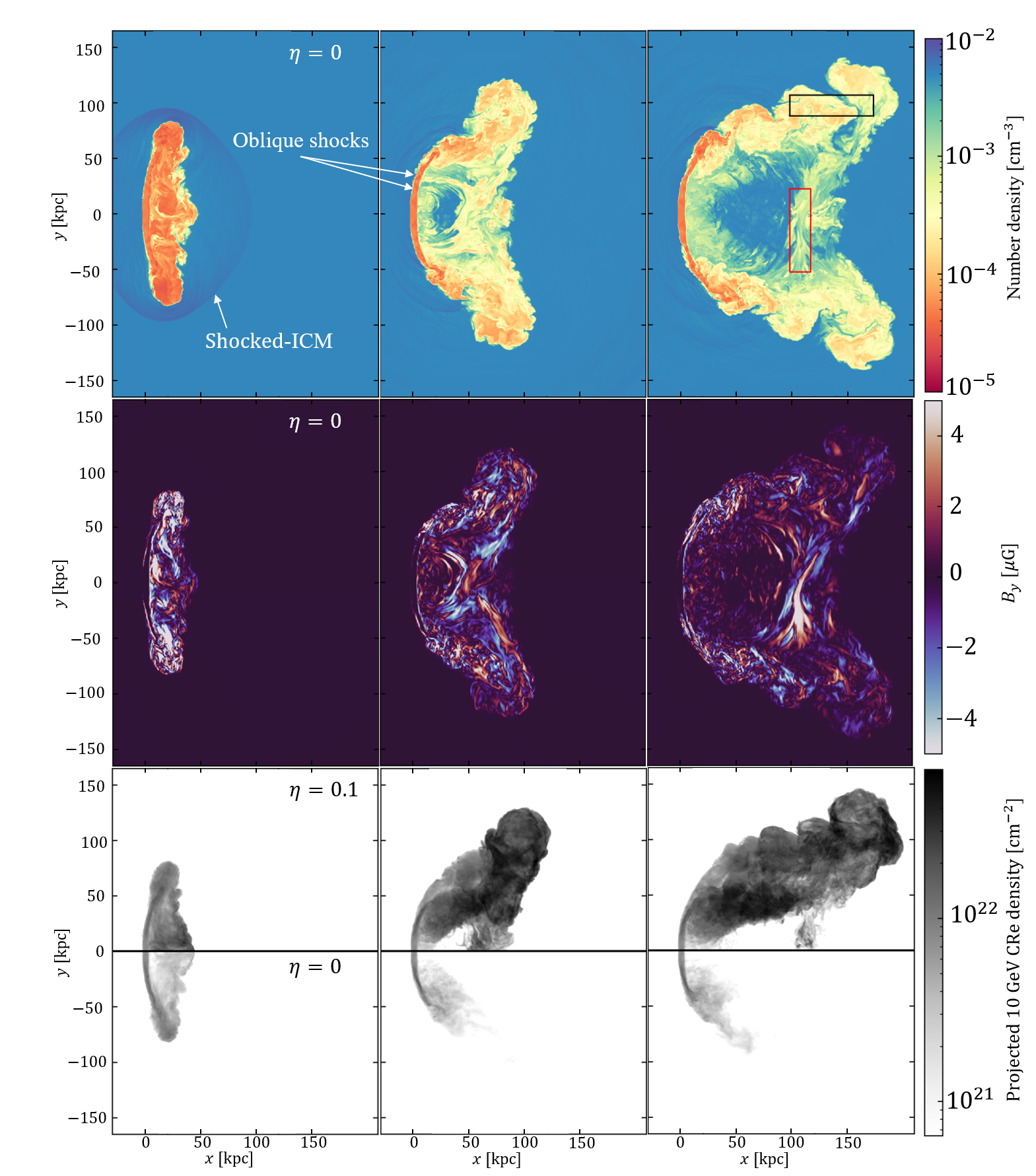
Figure 1: Number density (top) and the magnetic field strength (middle) maps ($z=0$ kpc) at $t=96.6,$ 193.2, and 316.3 Myr (from left to right). The rectangles indicate the regions to compute the characteristic scales of magnetic field for the tail (black) and the threads (red) (see section 5). The bottom panels show maps of 10 GeV CRe column density, $\int N_{\rm e,10GeV}dz$, for $\eta=0$ (lower half) and 0.1 (upper half).

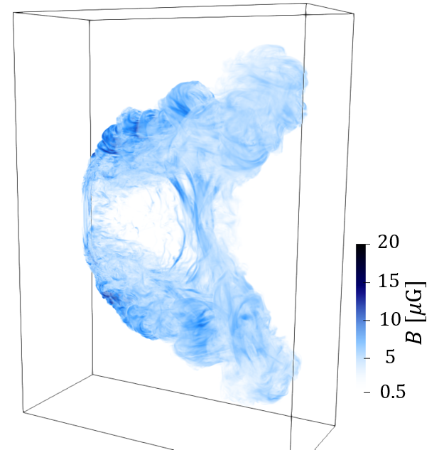
Figure 2: 3D render of magnetic field strength at $t=$ 316.3 Myr. The box size is $240\times 328\times 104$ ${\rm kpc^{3}}$.

The overall morphology and dynamics of the jets are similar to that discussed in previous simulations (Balsara & Norman, 1992; Porter et al., 2009; O’Neill et al., 2019). In Figure 1, we show snapshots of the number density, the magnetic field strength, and the projected 10 GeV CRe density at three different times $t=96.6$, 193.2, and 316.3 Myr. At early times, one can see the weak forward shock propagating into the ICM. The jet flows, which are heated up through the reverse shock (termination shock), decelerate and expand transversely. If there is no wind in the ambient ICM, these jets flow back symmetric along the jet axis and form ’cocoon’ (e.g., Norman et al., 1982). Since the backflow material is hot and light, the fluid is advected toward in the downwind direction. As a result, the jet material forms a ’U’ shape. Here, the important feature is that the backflowing plasma is connected to the opposite side of the jet tips. This phenomena is associated with the formation of magnetic threads in the later phase.

After the jet flow changes direction at the bending radius, $l_{\rm b}\sim 70$ kpc, by $\sim 90^{\circ}$ (see the middle panel of Figure 1), sub-sonic and super-Alfvenic turbulence are developed due to the growth of the Kelvin-Helmholtz (KH) instability between the lobe and the ICM. The weak oblique (recollimation) shocks are formed along the jet beams, and the jet velocity decreases through these shocks. The sonic Mach number of these shocks is about 2 so that the reveres shock may not lead sufficient shock acceleration. Beyond the point of maximum curvature along the jet axis, the flows are decelerated to sub-sonic velocities.

Since the pressure of the tail is greater than that of the surrounding ICM, the tail expands being mixed with ICM. One can see large vortices, whose diameter is about 30 - 50 kpc, in both the tails at $t=$ 316.3 Myr (the right panel of Figure 1). According to the discussion in O’Neill et al. (2019), the eddy turnover timescale can be roughly estimated as $\tau_{\rm eddy}\sim l_{\rm t}/v_{k,{\rm min}}\sim l_{\rm b}/v_{\rm w}\sim$ 80 Myr.

In our simulations, the magnetic field is provided only from the jet launching region. Since the plasma-$\beta$ for the jet, $\beta_{\rm jet}=20$, is high, the jet morphology is not affected by the magnetic force. We find that the magnetic field gradually decreases along the tail because the tail is expanding, and the diffusion and dissipation of the magnetic field occur at the boundary between tails and ICM. Note that in simulations the diffusion and dissipation of the magnetic field are numerically induced. We confirm that although the symmetrical boundary condition at $y=0$ does not affect the dynamics in the simulated results significantly by comparing the results for the symmetric and non-symmetric cases.

The bottom panels in Figure 1 show the effect of reacceleration for CRe. For $\eta=0.1$, the radio-emitting CRe, whose typical energy is 10 GeV, appear even at the end of the tail. The CRe are accumulated around the region of $|y|<50$ kpc, where the small-scale KH vortices are well developed. However, the magnetic field of this region is lower than that of the jets (see Figure 2). On the other hand, for $\eta=0$, there is no 10 GeV CRe in the tail. Since the cooling time for 10 GeV at $B=8$ $\mu$G is $\sim$ 170 Myr, the first injected CRe are already cooled at $t=193.2$ Myr (see the lower middle column in Figure 1).

3.2 Formation of magnetic threads

Figure 2 shows magnetic field threads connecting the two tails. Similar structures are also formed in the simulations of O’Neill et al. (2019) and Nolting et al. (2022), but the threads in our simulations are thinner and collimated, because of the high-spatial resolution scheme. The two large threads have opposite $y$-direction magnetic field. The radius and length of these threads are about 10 kpc and 150 kpc at $t=316.3$ Myr, respectively. The threads have relatively strong magnetic field, compared to that of the tail region. As we have pointed out, the backflowing materials at the initial stage are the origin of the magnetic threads. The threads dynamically evolve with the wind, i.e., the backflowing materials are advected by the wind forming the threads.

To clarify this point, we examine the time evolutions of the positions of the two threads. The average $y$-direction magnetic field in each grid point $(i,j,k)$ is calculated as

$$\bar{B}_{y}=\frac{1}{11^{2}}\sum^{i+5}_{i^{\prime}=i-5}\sum^{k+5}_{k^{\prime}=k-5}B_{y,(i^{\prime},j,k^{\prime})},$$ (15)

by averaging magnetic field $\pm 10$ grids in $x$ and $z$ directions. Then, we define the positions of the rich magnetic threads as the position where $|\bar{B}_{y}|$ is the maximum at $y=0$ plane. As shown in Figure 3, the advection velocities of both the threads are almost the same as the wind velocity after $t=100$ Myr.

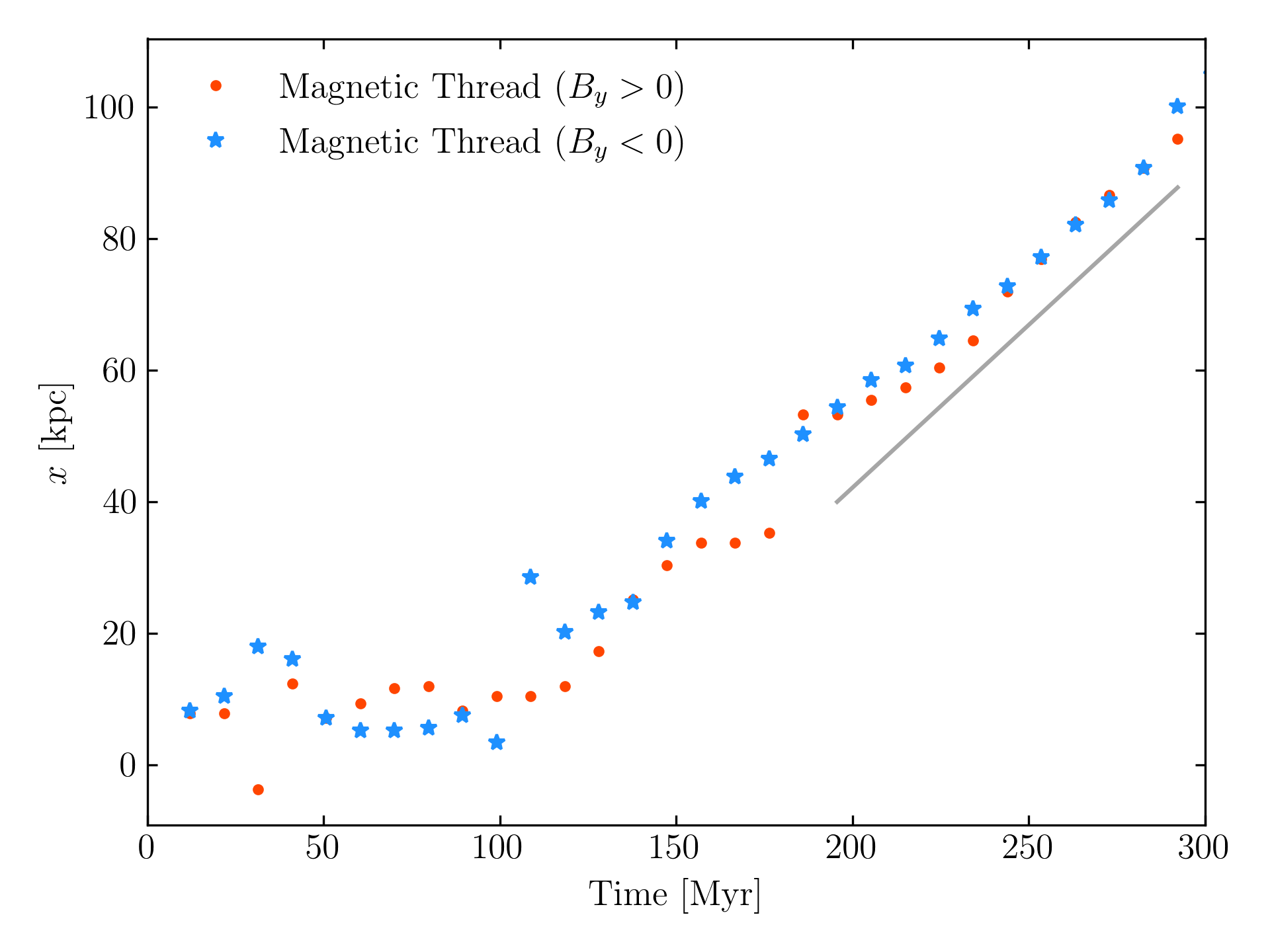
Figure 3: The time evolutions of the positions of the two magnetic threads at $y=0$. The gray line shows the wind motion, $x=v_{\rm ICM}t$

3.3 CRe and CRp energy evolution

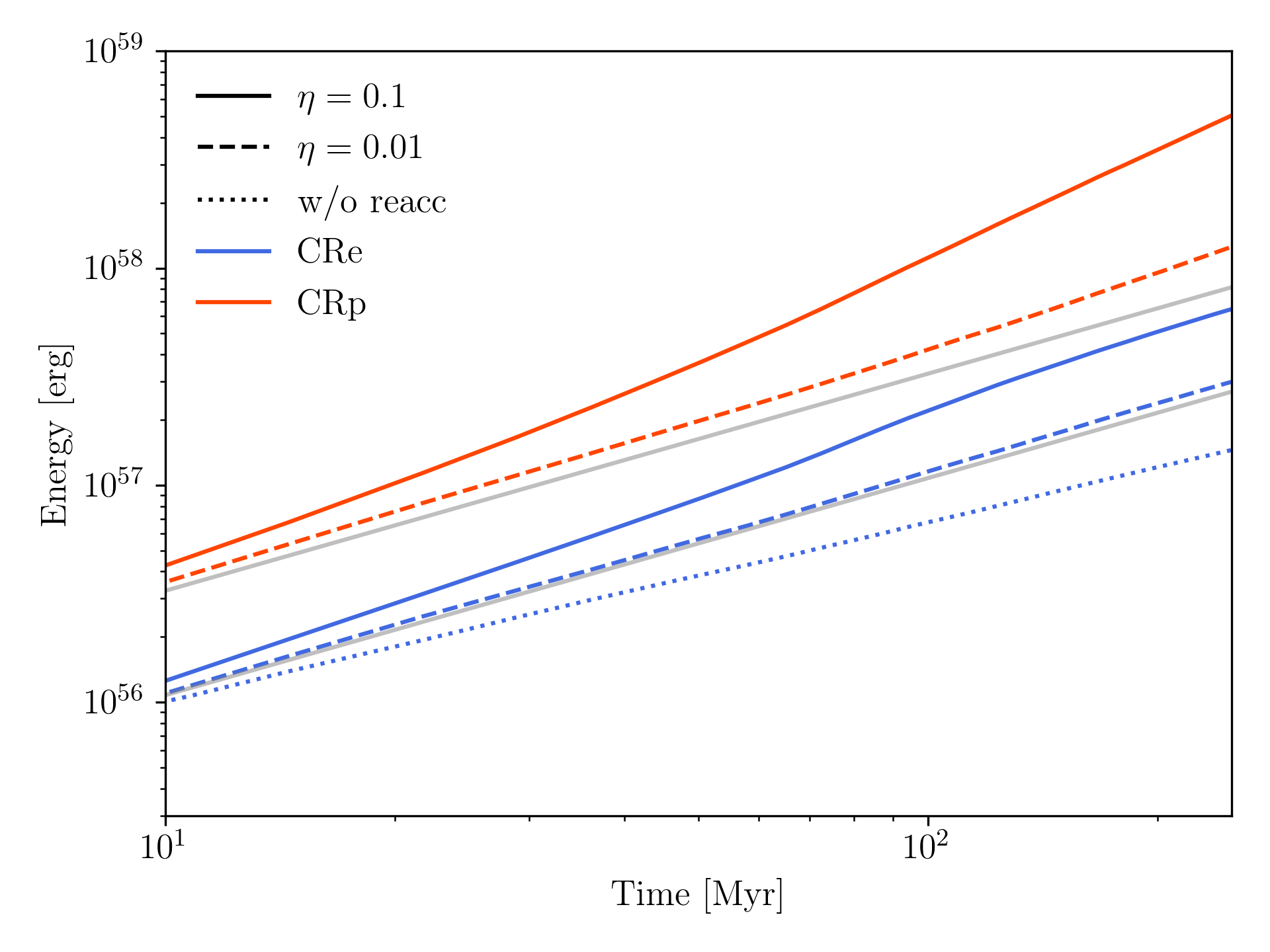
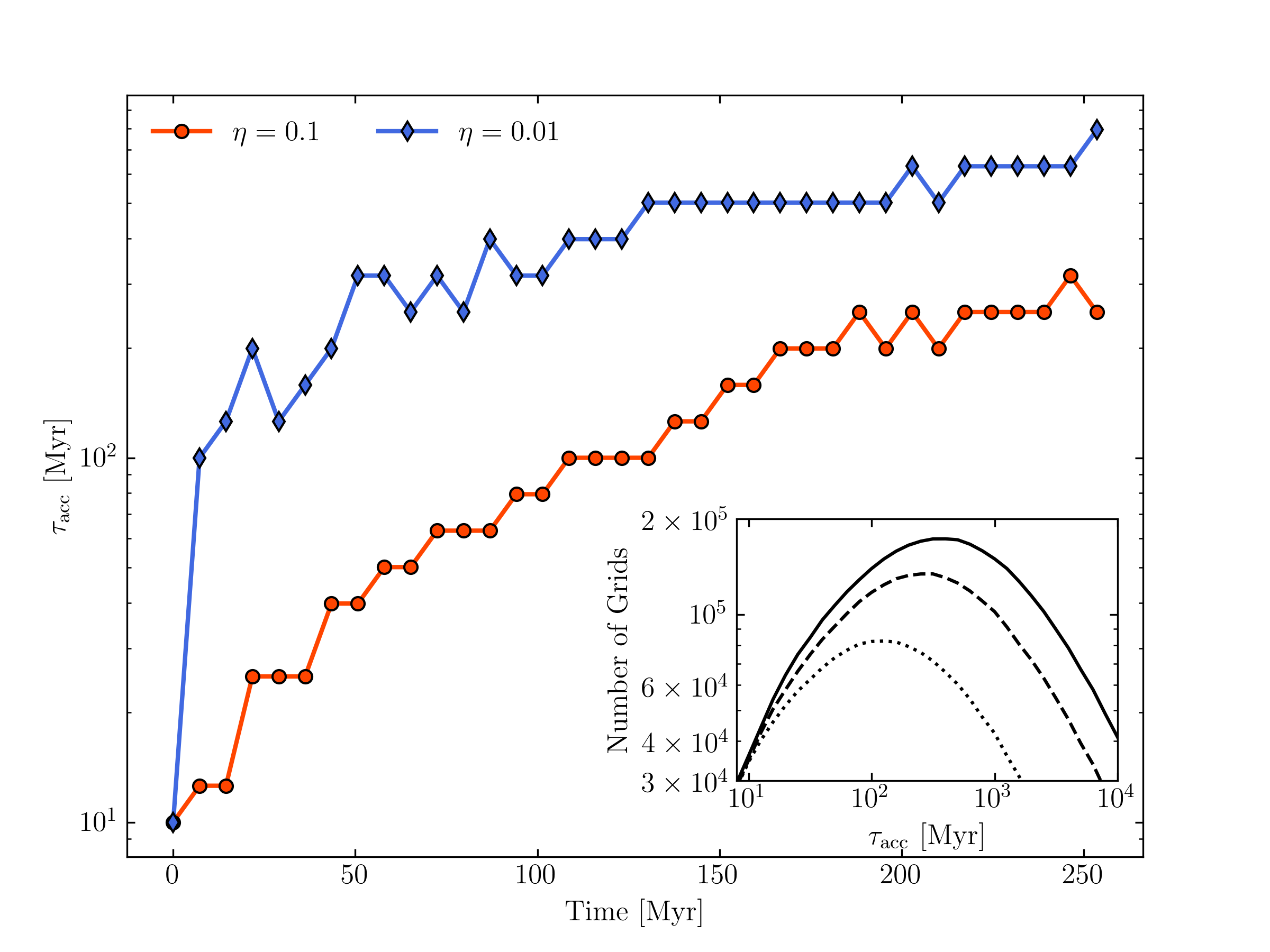
Figure 4: Left: Time evolutions of the energies of CRe (blue) and CRp (red) in the systems for $\eta=0$ (dotted), $0.01$ (dashed), and $0.1$ (solid). The gray solid lines are the expected growth of the CRe and CRp energies without energy gain and loss processes. Right: Time evolutions of the mode value of the acceleration timescales for $\eta=0.01$ (blue diamond) and $0.1$ (red circle). The inlet shows the distributions of the acceleration timescales at $t=$ 96.6 (dotted), 193.2 (dashed), and 316.3 (solid) Myr for $\eta=0.01$.

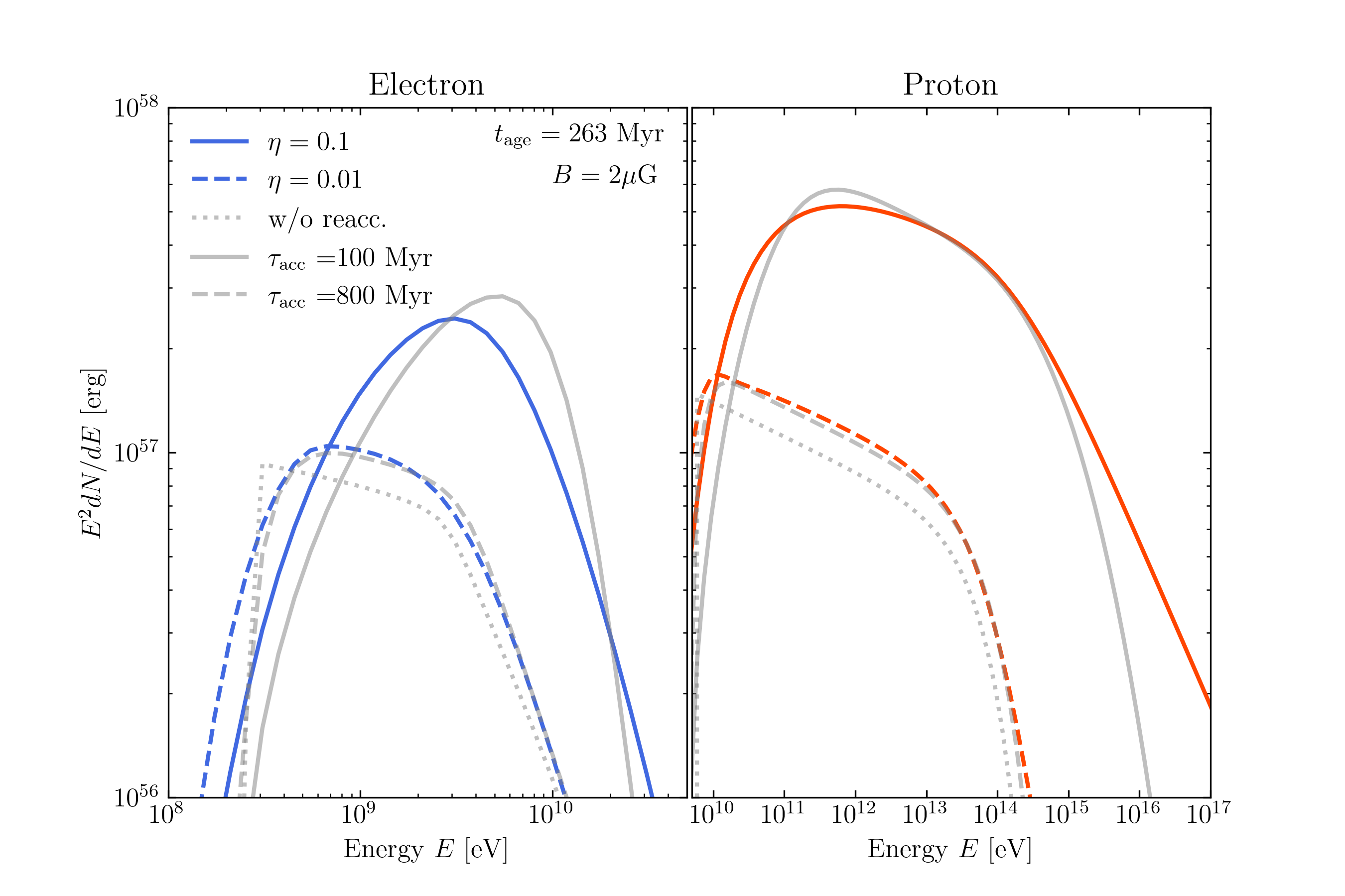
Figure 5: The CRe (left) and CRp (right) energy distributions integrated over the whole region for $\eta=0.01$ (dashed) and 0.1 (solid) at $t=316.3$ Myr. The gray lines show the spectra for the one-zone model with $\tau_{\rm acc}=$ 100 (solid), 800 (dashed), and $\infty$ (dotted) Myr, respectively.

The CRp and CRe energies evolve as shown in Figure 4. As mentioned in section 2.3, the effective value of $\eta$ is larger than the values we set. Our simulations show that 3 % and 30 % of the jet kinetic energy, $E_{\rm jet}=L_{\rm kin}t\sim 2.0\times 10^{59}$ erg, is converted into the CR particles energy at 316.3 Myr for $\eta=0.01$ and $0.1$, respectively. We check that the effective efficiencies $\eta^{\rm eff}\equiv\Delta E_{\rm CR}/E_{\rm diss}$, where $\Delta E_{\rm CR}$ and $E_{\rm diss}$ are respectively the energy gain of CR particles and the total dissipation energy, are $6.5\times 10^{-3}$ and $6.6\times 10^{-2}$ for $\eta=0.01$ and 0.1 at 316.3 Myr, respectively. This implies that the about 35 % of the gain energy is lost via radiation and adiabatic processes.

The acceleration timescale for CR particles is not constant, and depends on the total CR energy density and dissipated energy at each position. In Figure 4b, the acceleration timescales approximately follows a log-normal distribution. The mode value of the acceleration timescales monotonically increases and saturates at several hundred Myrs for both the models. There are two reasons for this trend. First, the volume of the tail increases with time, and also the turbulence decays along with the tail. As a result, the region with a lower dissipation rate expands. Since the flows around the bent region are supersonic, the dissipated energies are much larger than that around the tail region. Second, as the energy density of CR particles inceases, the acceleration timescale becomes longer.

Since CRe lose its energy by radiations, the growth rate of the CRe energy is lower than that of the CRp energy. For the case of $\eta=0.01$, the radiative energy loss is comparable to the energy gain due to reacceleration (see Figure 4), as the cooling timescale for GeV CRe is about 100 Myr in $\sim\mu$G magnetic field. Meanwhile, the energies of CRe and CRp for $\eta=0.1$ drastically increase because the jet age and the acceleration time are always comparable. The CRp energy of $\eta=0.1$ is about 10 times larger than that without reacceleration at $t=$ 316 Myr, while the CRe energy is slightly larger than that without reacceleration, because of the radiative cooling.

The CRe and CRp energy distributions integrated over the whole region are shown in Figure 5. For comparison, we calculated the time evolution of CR particles with a one-zone model, where we neglect the advection and the adiabatic terms in equations (1) and (2). We adopt a constant magnetic field 3 $\mu$G and thermal electron density of 0.01 ${\rm cm^{3}}$, and the acceleration times of 100 and 800 Myr for $\eta=0.01$ and 0.1. The results are shown by the gray lines in Figure 5. For $\eta=0.01$, the simulation and the one-zone model have similar energy distributions of CRe and CRp. While most of the acceleration timescales are longer than the age of the jet during the simulation, a small fraction of CRe accelerate very efficiently. In contrary to this, the energy distributions of both CRe and CRp for $\eta=0.1$ are significantly different from that of the one-zone model. At higher energies, the spectra in the simulations is much harder than those for the one-zone model (see Figure 4). Differently from the one-zone model, the scattered values of the energy dissipation rate in the MHD simulations broaden the CR spectra. In low-dissipation regions, the inefficient acceleration leads to the lower peak of the CR spectra. Alternatively, high-dissipation regions are the main sites where CRs in the high-energy tail are accelerated.

4 Radiation from head-tail galaxy

In this section, we discuss leptonic and hadronic emissions from our models. For calculating fluxes, the source luminosity distance is assumed as $D=$ 70 Mpc, which is roughly the same as the distance of NGC 1265 in the Perseus Cluster. The emissions are calculated by using the snap shot data at $t=316.3$ Myr. We assume that the tails lie in the plane of the sky for simplicity.

4.1 Radio emission

The integrated synchrotron flux densities are shown in Figure 6. In the model without reacceleration, the radio spectrum is almost a single power-law with an index of $\alpha\sim-0.9$. The index is slightly harder than the simple expectation from the continuous injection model, whose electron spectrum, $N(\gamma)\propto\gamma^{-p+1}$, i.e., $\alpha\sim-1.05$. That difference may come from the effect of adiabatic compression and the Coulomb loss. In contrast to this, the spectral indices for the models with reacceleration become softer as frequencies get higher. Above 5 GHz the radio spectra become harder reflecting the curved electron spectrum.

The physical sizes of our models are $\sim$ 200 kpc at the time in our mock observation, and the 150 MHz luminosities are $L_{\rm 150}=2.1\times 10^{32},~{}6.0\times 10^{32}$, and $1.5\times 10^{33}$ erg/Hz for $\eta=$ 0, 0.01, and 0.1, respectively. From the LOFAR Two-Metre Sky Survey, $L_{\rm 150}$ is in the ranges between $10^{31}$ and $10^{33}$ for the observed head-tail galaxies, whose physical size are about 200 kpc (Mingo et al., 2019). Thus, the model for $\eta=0.1$ corresponds to the most luminous radio source.

The 300 MHz radio maps and the spectral index map derived from the radio data at 150 - 600 MHz in our simulations are shown in Figure 7. We also show their profiles across the jets in Figure 8. The radio emission is most prominent at the end of the bending, where the magnetic field strength is high (see also Figure 1 and 2). Because of radiative cooling and adiabatic expansion, the brightness in the model without reacceleration is dark in the tail region. Although a large amount of CRe is accumulated in the tail region, such low-energy electrons do not radiate in the radio band. This behavior is the same as ones seen in the pure-aging scenario, that is inconsistent with radio observations (Jaffe & Perola, 1973).

In the presence of the reacceleration, the radio intensity in the tail region is so high that recent instruments can detect. The radio flux and spectral index do not change drastically. Those behaviors are consistent with some head tail galaxies (Pacholczyk & Scott, 1976; Miley et al., 1975; O’Dea & Owen, 1986; Feretti et al., 1998; Müller et al., 2021). The profiles of the radio flux and the spectral index for $\eta=0.01$ and 0.1 have similar trends, while the efficiency of the reacceleration affects the normalization. Thus, it may be difficult to determine the value of $\eta$ from the radio intensity distribution. Meanwhile, the spectral index offers a hint. Recent radio observations show that the spectral index for hundreds of MHz frequency range is -1.0 or less in the tails (Sebastian et al., 2017; Gendron-Marsolais et al., 2020). Therefore, the spectral index fro $\eta=0.1$ may be too hard.

Our simulation shows the rich magnetic threads. However, the radio emission from this threads is not identified in the radio maps, because CRe in this region are already cooled and those CRe are not accelerated efficiently due to lower dissipation energies in this region. An additional mechanism is needed to produce radio threads. The detailed discussion of the radio threads is described in the section 5.

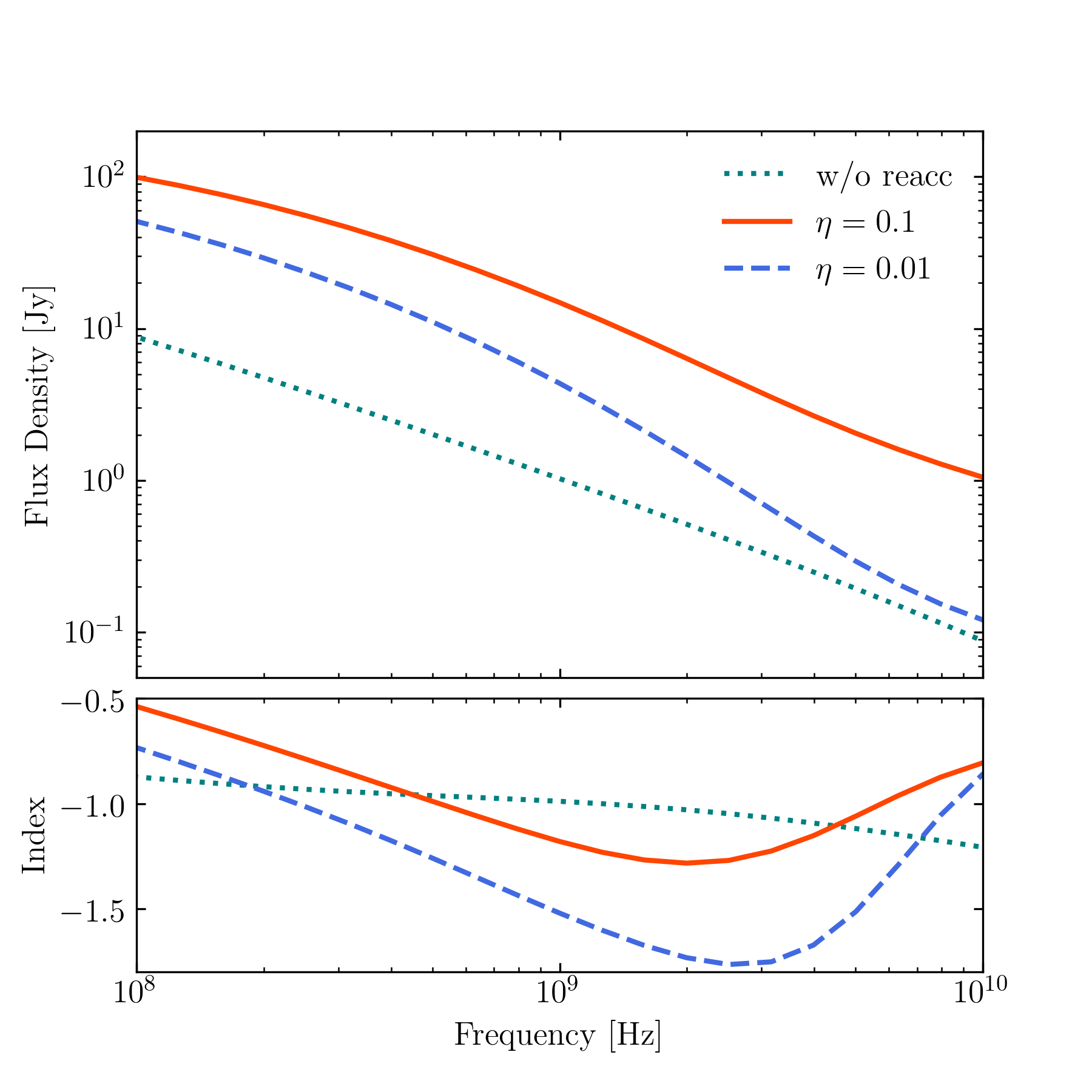
Figure 6: Integrated radio spectra for $\eta=0$ (green dotted), 0.01 (blue dashed), and 0.1 (red solid).

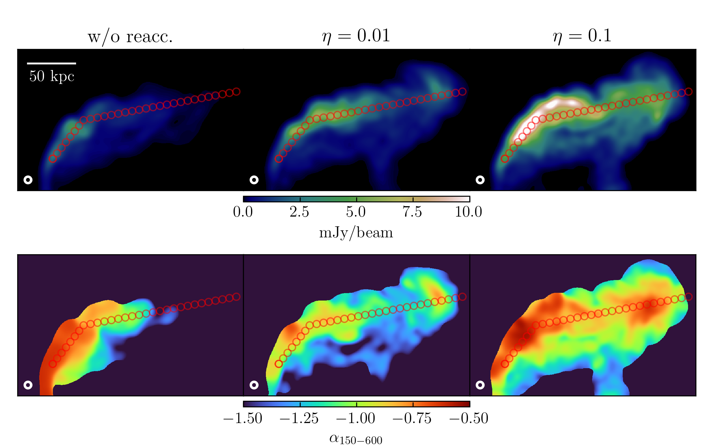
Figure 7: top: 300 MHz radio maps for $\eta=$ 0, 0.01, and 0.1 (from left to right). The source luminosity distance is assumed as $D=$ 70 Mpc. The beam size, 7” $\times$ 7”, is shown in the bottom left corner. Red circles on the radio jet indicate the position where the fluxes are estimated in Figure 8. bottom: Spectral index maps derived from the radio data obtained at 150 - 600 MHz.

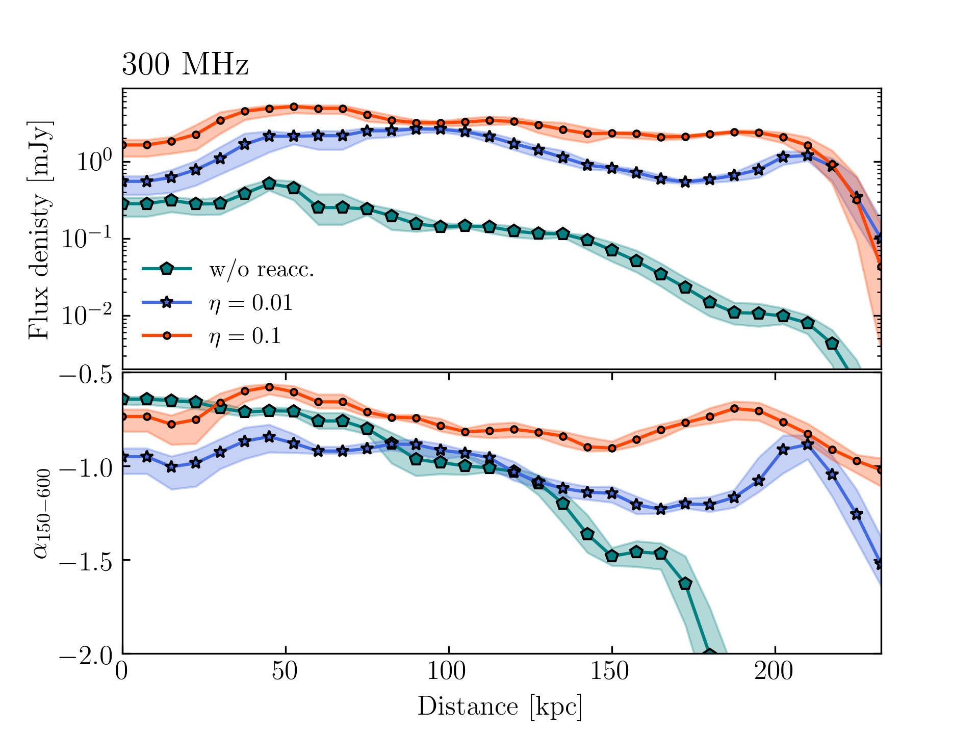
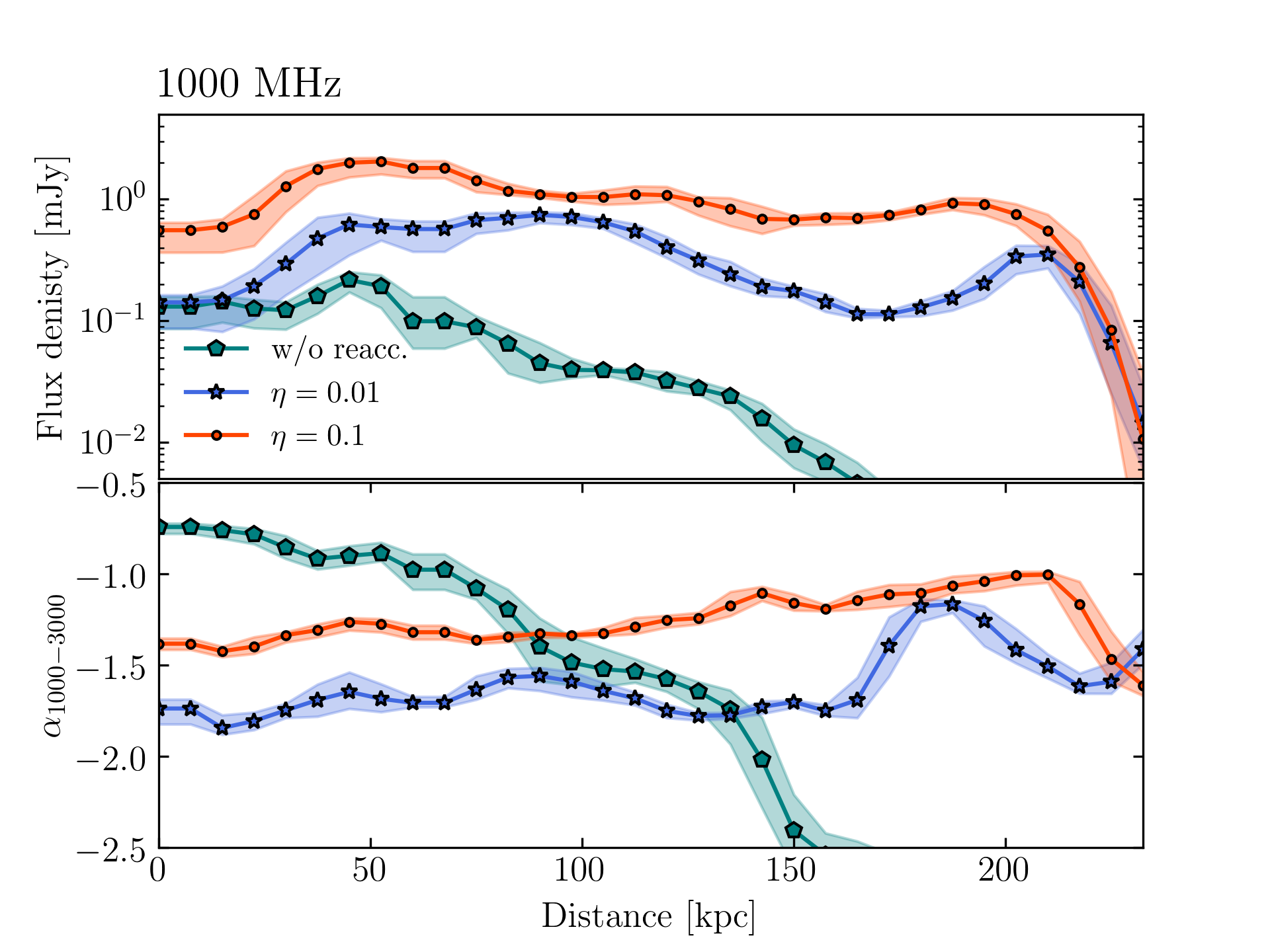
Figure 8: Flux densities (top panels) and spectral indices (bottom panels) profiles along the radio jets indicated in Figure 7 for $\eta=0$ (green hexagons), 0.01 (blue stars), and 0.1 (red circles).

4.2 Non-thermal X-ray emission

Figure 9 (left) shows the 20 keV X-ray map for $\eta=0.1$. The typical Lorentz factor of 20 keV X-ray emitting electrons by inverse Compton scattering is $\gamma_{\rm IC}\sim 6000$. The hard X-ray is the brightest in the termination of the radio tail, where the accelerated CRe are accumulated (see also the bottom right panel of Figure 1). This result is different from the radio morphology (see Figure 7), which is brightest at the bending point.

To discuss the detectability with the future X-ray mission, Focusing On Relativistic universe and Cosmic Evolution (FORCE) (Mori et al., 2016), we derive X-ray spectra integrated within the field of view (FOV) of FORCE (Figure 9). FORCE has $\sim$ 15” angular resolution, and thus has high sensitivity of $3\times 10^{-15}$ ${\rm erg~{}cm^{-2}~{}s^{-1}~{}keV^{-1}}$ for 1 Ms observations in the range of 10 to 40 keV for point-like sources (Nakazawa et al., 2018). As shown in Figure 9 (right), hard X-ray emissions from radio tail can be detected when electrons are reaccelerated efficiently. Since the FORCE target sensitivity for diffuse sources is lower than that for point-like sources, it might be hard to detect hard X-ray emission for the case of inefficient reacceleration ($\eta<0.01$).

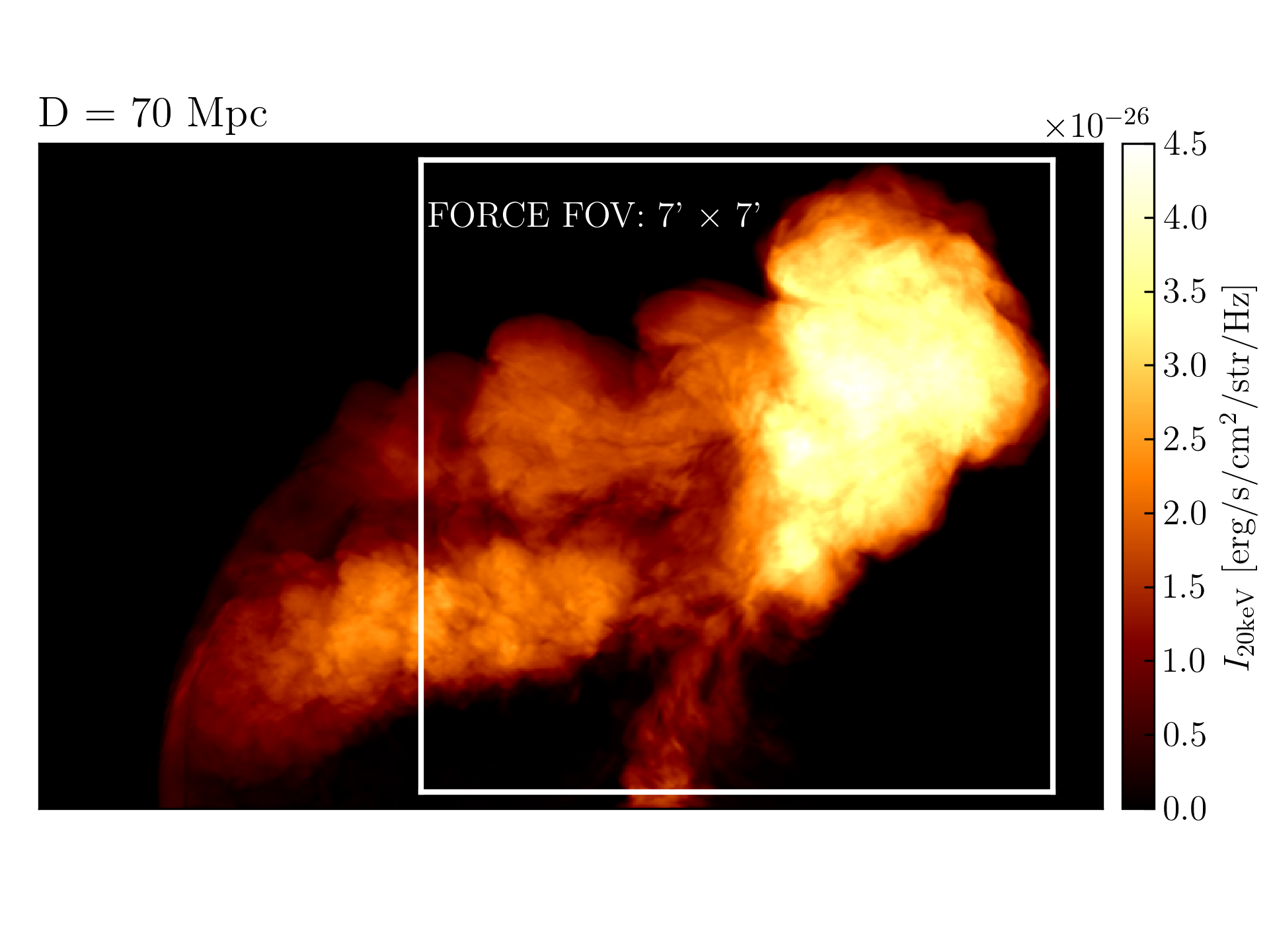
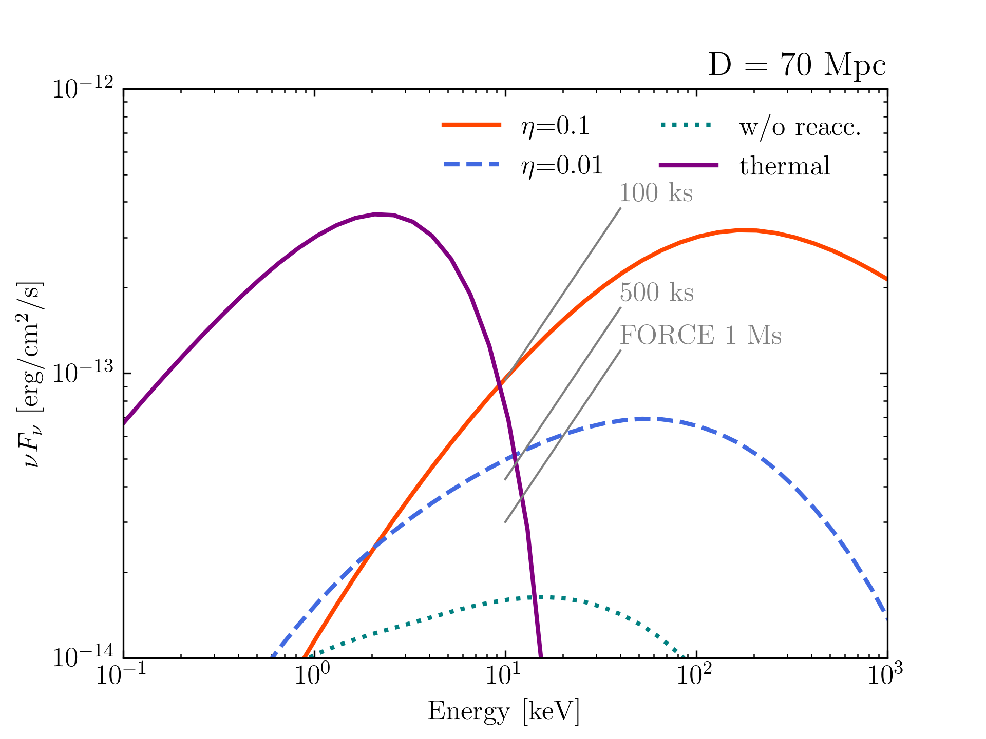
Figure 9: left: 20 keV X-ray map for $\eta=0.1$. The square corresponds to the FOV of FORCE at a distance of 70 Mpc. right: X-ray spectra within the FOV of FORCE. The dashed blue line and solid red line show non-thermal X-ray spectra of inverse Compton scattering for $\eta=0.01$ and $0.1$, respectively. The purple solid line shows the thermal X-ray emission from 5 keV ICM. The gray lines illustrate the target sensitivity of FORCE with 100 ks, 500 ks, and 1 Ms of observation time (Nakazawa et al., 2018).

4.3 Gamma-ray and neutrino emissions

We show gamma and neutrino spectra for $\eta=0.01$ and $0.1$ in Figure 10. The fluxes are calculated as a point source at $D=70$ Mpc. Note that, for simplicity, the extragalactic background light absorption, which is significant above 100 GeV, is ignored. These fluxes are more than three orders of magnitude below the upper limits of the Fermi-LAT and the IceCube.

Comparing with the spectra for the one-zone model (see detail in section 3.3), our MHD models show harder spectra, especially for $\eta=0.1$. Note that the normalization of the one-zone model is adjusted to visualize the differences clearly in Figure 10. Because turbulence develops around the contact discontinuity, CR particles are efficiently accelerated in these regions. The gas density is also higher due to mixing of the ICM and the jet gas. Therefore, contributions from such regions are dominant in the final spectra.

Only one candidate gamma-ray source has been found for head-tail galaxies. Neronov et al. (2010) reported that very high energy gamma-ray photons come from the head-tail galaxy IC 310. However, its core has a blazer-like radio structure (Kadler et al., 2012), i.e., the jet orients close to the line of sight. Thus, high-energy TeV photons most likely originate from the core region. Our result is compatible with this interpretation.

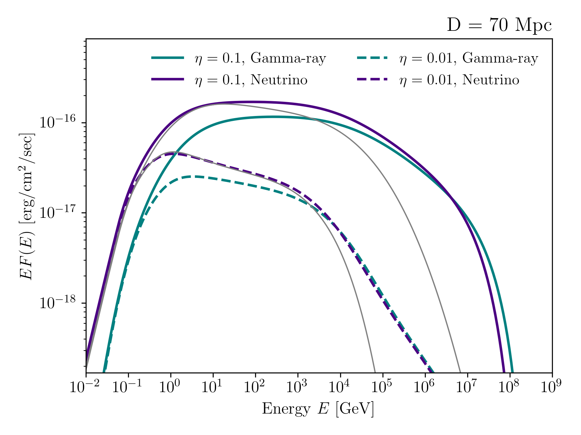
Figure 10: $\pi^{0}$ gamma (green) and neutrino (purple) spectra for $\eta=0.01$ (dashed) and 0.1 (solid). The gray lines show the neutrino spectra of the one-zone model with $\tau_{\rm acc}=$ 100 (upper) and 800 (lower) Myr.

5 spatial diffusion of electrons in the magnetic threads

Our simulations show that head-tail galaxies have magnetic threads linking the two tails (see Figure 2). However, the radio intensity from these threads is lower than sensitivities of recent radio detectors (Ramatsoku et al., 2020). In this section, we dicsuss the spatial diffusion effect, neglected in our simulations, on the radio brightness of the magnetic threads. High-energy electrons penetrating into the threads would produce radio threads that can be identified with observations.

First, we calculate the characteristic scales of magnetic field in the parallel and perpendicular in the magnetic threads and tails as follows (Schekochihin et al., 2004; Bodo et al., 2011)

$$l_{\parallel}=\sqrt{\frac{\langle\bm{B}^{4}\rangle}{\langle|\bm{B}\cdot\nabla\bm{B}|^{2}\rangle}},$$ (16)

$$l_{\perp}=\sqrt{\frac{\langle\bm{B}^{4}\rangle}{\langle|\bm{B}\times\bm{J}|^{2}\rangle}},$$ (17)

where $\bm{J}=\nabla\times\bm{B}$, and $\langle\rangle$ denotes a volume average. The spatial regions for the average are shown by the rectangles in Figure 1. The tail and threads have similar values of $l_{\perp}$, 1.35 kpc and 1.71 kpc, respectively. In contrast to this, we can see the magnetic structures of the threads are more anisotropic than that of the tail. The values of $l_{\parallel}$ are 3.99 kpc for tails and 9.88 kpc for threads. Here, we note that a highly anisotropy with $l_{\parallel}/l_{\perp}>10$ can be seen when we cut out a small region focusing on the large magnetic threads.

First, we discuss the spatial diffusion of CRe. Based on the result of the previous paragraph, we assume that CRe can diffuse only along the flux-tube. Typical value of magnetic field in the threads is 5 $\mu$G, and hence the cooling time for 10 GeV electrons is $\tau_{\rm cool}\sim 170$ Myr. The diffusion length can be written as $l_{\rm diff}\sim 2\sqrt{D_{\parallel}t}$ in a time $t$, where $D_{\parallel}$ is the spatial diffusion coefficient. Thus, the spatial diffusion coefficient along the flux tube required for transportation of CRe to shine the threads, whose half length is about 70 kpc, within the cooling time is $\sim 2.1\times 10^{30}$ $\rm cm^{2}/s$.

Considering the spatial diffusion via the gyroresonant interaction, the spatial diffusion coefficient can be written as (Kulsrud & Pearce, 1969)

$$D_{\parallel}=\frac{1}{3}cr_{\rm g}\quantity(\frac{B^{2}_{\parallel}}{k_{\rm g}W_{B_{\perp}}(k_{\rm g})}),$$ (18)

where $r_{\rm g},~{}k_{\rm g}$ and $W_{B_{\perp}}$ are the Larmor radius of the CRe, $k_{\rm g}=2\pi r^{-1}_{\rm g}$, and the turbulent spectrum of the perpendicular magnetic field, respectively. We compute the volume average parallel magnetic field in the region of the thread as

$$\bar{B_{\parallel}}=\frac{\int B_{y}N_{\rm e,100MeV}\differential{V}}{\int N_{\rm e,100MeV}\differential{V}}=4.8~{}\mu{\rm G},$$ (19)

and the average perpendicular magnetic field as

$$\bar{B_{\perp}}(y)=\frac{\int\int B_{\perp}N_{\rm e,100MeV}\differential{x}\differential{z}}{\int\int N_{\rm e,100MeV}\differential{x}\differential{z}},$$ (20)

where $B_{\perp}=\sqrt{B_{x}^{2}+B_{z}^{2}}$. Then, we calculate the turbulence spectrum by using the Fourier transform of $\bar{B_{\perp}}(y)$. We find that the index of the turbulence spectrum is close to the Kolmogorov scaling, $W_{B_{\perp}}\propto k^{-5/3}$. Since the Larmor radius of 10 GeV electrons is much smaller than the MHD grid size, the resonant occurs at the sub-grid scale. Therefore, we extrapolate the turbulence spectrum extrapolating the Kolmogorov scaling to estimate $D_{\parallel}$ for 10 GeV electrons. As a result, we obtain $D_{\parallel}\sim 10^{32}~{}{\rm cm^{2}/s}$ from equation (18). This value is two orders of magnitude larger than that required for the transportation of CRe. Meanwhile, this discussion is optimistic in the sense of assuming that the flux tube completely lies in the y-direction, i.e., the flux tube is not tangled. The average procedure with equation (20) may also lead to an underestimated amplitude of the local turbulence.

In addition to the spatial diffusion, ”CR streaming” is often invoked as another transport mechanism of CR particles (Kulsrud & Pearce, 1969). The CR particles can stream along the magnetic field line with Alfvén waves, and it is generally known that the streaming velocity $v_{\rm st}$ is limit to Alfvén velocity $v_{\rm A}(=B/\sqrt{4\pi\rho})$. Optimistically, we adopt $B=5~{}\mu{\rm G},\rho=1.0\times 10^{-3}m_{\rm p}$ and $v_{\rm st}=v_{\rm A}\sim 335$ km/s. So that the length that CRe can stream along the flux tube in $\tau_{\rm cool}$ is $l_{\rm st}=v_{\rm A}\tau_{\rm cool}\sim 67$ kpc, which is comparable to the length of threads. This simple estimate implies that the CR streaming could also be the important process for the formation of synchrotron threads.

6 Summary and discussion

We have performed the 3D CR MHD simulations of a head-tail galaxy, focusing on reacceleration of CR particles and non-thermal emissions. Because the scale at which CR particles interact with turbulence is much smaller than the resolution of our simulations, we estimate the efficiency of reacceleration with a sub-grid recipe to bride this scale gap. In this paper, we adopt the hard-sphere type acceleration model with a parameter $\eta$, that adjusts the energy conversion efficiency from dissipation energy to the CR particle energy. The main results of this study are summarized as follows:

• Depending on the values of $\eta$, 3 - 30 % of the jet kinetic energy is converted into CR particles energy at $t=316.3$ Myr. Our global simulations show significantly different CR spectra from those in simple one-zone models.

• In the presence of reacceleartion, the radio flux and spectral index do not decrease along with the tails. Those behaviors are consistent with some head-tail galaxies, and therefore reacceleration is essential. For $\eta=0.1$, the spectral index for hundreds of MHz frequency ranges is harder than that for $\eta=0.01$ and the radio observations.

• Inverse Compton X-ray emission from head-tail galaxies in the Perseus Cluster can be observed by the future X-ray observatory (FORCE). On the other hand, hadronic gamma-ray and neutrino emissions are too dim to be detected with the current instruments.

• Thin magnetic field threads connecting the two tails are identified in our simulations. The origin of these threads is backflow at early phase. The backflowing materials are simply advected by the wind to form the threads.

• An efficient transport mechanism of CRe is needed to explain the observed radio threads. Considering the spatial diffusion process of CRe along the threads, $D_{\parallel}\sim 2.1\times 10^{30}$ $\rm cm^{2}/s$ is required.

This study is our first step in constructing a realistic model to implement the reacceleration process with MHD simulations, and there are several important limitations in our current models. First, our code do not account for the dynamical back-reaction from CR particles. The CR energy density is comparable to the thermal energy density for $\eta=0.1$. Therefore, the CR pressure may be dynamically significant.

Second, the spatial diffusion and streaming would affect the radio emission map. As discussed in section 5, it would be important for the formation of synchrotron threads. Meanwhile, in the tail regions, the magnetic field is highly tangled so that the spatial diffusion may be suppressed in such disturbed regions. This picture has been supported by early MHD simulations of radio jets (Ehlert et al., 2018).

Additionally, subsequent particle injection has been neglected. O’Neill et al. (2019) showed that weak shocks in the tail region is too weak to inject particles. However, the shock acceleration can be dominant process in high power jets. As future extension of this study we should implement those processes in a self-consistently manner (e.g., Girichidis et al., 2020; Ogrodnik et al., 2021; Böss et al., 2022).

References

- Asahina et al. (2014) Asahina, Y., Ogawa, T., Kawashima, T., et al. 2014, ApJ, 789, 79
- Balsara & Norman (1992) Balsara, D. S., & Norman, M. L. 1992, ApJ, 393, 631
- Begelman et al. (1979) Begelman, M. C., Rees, M. J., & Blandford, R. D. 1979, Nature, 279, 770
- Bicknell (1984) Bicknell, G. V. 1984, ApJ, 286, 68
- Bodo et al. (2011) Bodo, G., Cattaneo, F., Ferrari, A., Mignone, A., & Rossi, P. 2011, ApJ, 739, 82
- Böss et al. (2022) Böss, L. M., Steinwandel, U. P., Dolag, K., & Lesch, H. 2022, arXiv e-prints, arXiv:2207.05087
- Brunetti & Jones (2014) Brunetti, G., & Jones, T. W. 2014, International Journal of Modern Physics D, 23, 1430007
- Brunetti & Lazarian (2007) Brunetti, G., & Lazarian, A. 2007, MNRAS, 378, 245
- Brunetti et al. (2001) Brunetti, G., Setti, G., Feretti, L., & Giovannini, G. 2001, MNRAS, 320, 365
- Chibueze et al. (2021) Chibueze, J. O., Sakemi, H., Ohmura, T., et al. 2021, Nature, 593, 47
- Croston & Hardcastle (2014) Croston, J. H., & Hardcastle, M. J. 2014, MNRAS, 438, 3310
- de Gasperin et al. (2017) de Gasperin, F., Intema, H. T., Shimwell, T. W., et al. 2017, Science Advances, 3, e1701634
- Dedner et al. (2002) Dedner, A., Kemm, F., Kröner, D., et al. 2002, Journal of Computational Physics, 175, 645
- Donnert & Brunetti (2014) Donnert, J., & Brunetti, G. 2014, MNRAS, 443, 3564
- Edler et al. (2022) Edler, H. W., de Gasperin, F., Brunetti, G., et al. 2022, A&A, 666, A3
- Ehlert et al. (2018) Ehlert, K., Weinberger, R., Pfrommer, C., Pakmor, R., & Springel, V. 2018, MNRAS, 481, 2878
- Feretti et al. (1998) Feretti, L., Giovannini, G., Klein, U., et al. 1998, A&A, 331, 475
- Fermi (1949) Fermi, E. 1949, Phys. Rev., 75, 1169. https://link.aps.org/doi/10.1103/PhysRev.75.1169
- Fouka & Ouichaoui (2013) Fouka, M., & Ouichaoui, S. 2013, Research in Astronomy and Astrophysics, 13, 680
- Fujita et al. (2015) Fujita, Y., Takizawa, M., Yamazaki, R., Akamatsu, H., & Ohno, H. 2015, ApJ, 815, 116
- Gan et al. (2017) Gan, Z., Li, H., Li, S., & Yuan, F. 2017, ApJ, 839, 14
- Gendron-Marsolais et al. (2020) Gendron-Marsolais, M., Hlavacek-Larrondo, J., van Weeren, R. J., et al. 2020, MNRAS, 499, 5791
- Girichidis et al. (2020) Girichidis, P., Pfrommer, C., Hanasz, M., & Naab, T. 2020, MNRAS, 491, 993
- Gould (1972) Gould, R. 1972, Physica, 60, 145. https://www.sciencedirect.com/science/article/pii/0031891472902273
- Govoni & Feretti (2004) Govoni, F., & Feretti, L. 2004, International Journal of Modern Physics D, 13, 1549
- Hardcastle et al. (2002) Hardcastle, M. J., Birkinshaw, M., Cameron, R. A., et al. 2002, ApJ, 581, 948
- Hardcastle et al. (2004) Hardcastle, M. J., Harris, D. E., Worrall, D. M., & Birkinshaw, M. 2004, ApJ, 612, 729
- Hardcastle & Worrall (2000) Hardcastle, M. J., & Worrall, D. M. 2000, MNRAS, 319, 562
- Ignesti et al. (2022) Ignesti, A., Brunetti, G., Shimwell, T., et al. 2022, A&A, 659, A20
- Inoue & Takahara (1996) Inoue, S., & Takahara, F. 1996, ApJ, 463, 555
- Jaffe & Perola (1973) Jaffe, W. J., & Perola, G. C. 1973, A&A, 26, 423
- Jones (1968) Jones, F. C. 1968, Physical Review, 167, 1159
- Jones & Kang (2005) Jones, T. W., & Kang, H. 2005, Astroparticle Physics, 24, 75
- Jones & Owen (1979) Jones, T. W., & Owen, F. N. 1979, ApJ, 234, 818
- Kadler et al. (2012) Kadler, M., Eisenacher, D., Ros, E., et al. 2012, A&A, 538, L1
- Kamae et al. (2006) Kamae, T., Karlsson, N., Mizuno, T., Abe, T., & Koi, T. 2006, ApJ, 647, 692
- Kamae et al. (2007) —. 2007, ApJ, 662, 779
- Kelner et al. (2006) Kelner, S. R., Aharonian, F. A., & Bugayov, V. V. 2006, Phys. Rev. D, 74, 034018
- Knowles et al. (2022) Knowles, K., Cotton, W. D., Rudnick, L., et al. 2022, A&A, 657, A56
- Kulsrud & Pearce (1969) Kulsrud, R., & Pearce, W. P. 1969, ApJ, 156, 445
- Kundu et al. (2021) Kundu, S., Vaidya, B., & Mignone, A. 2021, ApJ, 921, 74
- Kundu et al. (2022) Kundu, S., Vaidya, B., Mignone, A., & Hardcastle, M. J. 2022, A&A, 667, A138
- Matsumoto & Masada (2019) Matsumoto, J., & Masada, Y. 2019, MNRAS, 490, 4271
- Matsumoto et al. (2019) Matsumoto, Y., Asahina, Y., Kudoh, Y., et al. 2019, PASJ, 71, 83
- Mertsch & Sarkar (2011) Mertsch, P., & Sarkar, S. 2011, Phys. Rev. Lett., 107, 091101
- Miley et al. (1972) Miley, G. K., Perola, G. C., van der Kruit, P. C., & van der Laan, H. 1972, Nature, 237, 269
- Miley et al. (1975) Miley, G. K., Wellington, K. J., & van der Laan, H. 1975, A&A, 38, 381
- Mimica et al. (2009) Mimica, P., Aloy, M. A., Agudo, I., et al. 2009, ApJ, 696, 1142
- Mingo et al. (2019) Mingo, B., Croston, J. H., Hardcastle, M. J., et al. 2019, MNRAS, 488, 2701
- Miyoshi & Kusano (2005) Miyoshi, T., & Kusano, K. 2005, Journal of Computational Physics, 208, 315
- Mori et al. (2016) Mori, K., Tsuru, T. G., Nakazawa, K., et al. 2016, in Society of Photo-Optical Instrumentation Engineers (SPIE) Conference Series, Vol. 9905, Space Telescopes and Instrumentation 2016: Ultraviolet to Gamma Ray, ed. J.-W. A. den Herder, T. Takahashi, & M. Bautz, 99051O
- Müller et al. (2021) Müller, A., Pfrommer, C., Ignesti, A., et al. 2021, MNRAS, 508, 5326
- Nakazawa et al. (2018) Nakazawa, K., Mori, K., Tsuru, T. G., et al. 2018, in Society of Photo-Optical Instrumentation Engineers (SPIE) Conference Series, Vol. 10699, Space Telescopes and Instrumentation 2018: Ultraviolet to Gamma Ray, ed. J.-W. A. den Herder, S. Nikzad, & K. Nakazawa, 106992D
- Neronov et al. (2010) Neronov, A., Semikoz, D., & Vovk, I. 2010, A&A, 519, L6
- Nishiwaki & Asano (2022) Nishiwaki, K., & Asano, K. 2022, ApJ, 934, 182
- Nishiwaki et al. (2021) Nishiwaki, K., Asano, K., & Murase, K. 2021, ApJ, 922, 190
- Nolting et al. (2022) Nolting, C., Lacy, M., Croft, S., et al. 2022, arXiv e-prints, arXiv:2206.04757
- Norman et al. (1982) Norman, M. L., Winkler, K. H. A., Smarr, L., & Smith, M. D. 1982, A&A, 113, 285
- O’Dea & Owen (1986) O’Dea, C. P., & Owen, F. N. 1986, ApJ, 301, 841
- Ogrodnik et al. (2021) Ogrodnik, M. A., Hanasz, M., & Wóltański, D. 2021, ApJS, 253, 18
- Ohmura et al. (2020) Ohmura, T., Machida, M., Nakamura, K., Kudoh, Y., & Matsumoto, R. 2020, MNRAS, 493, 5761
- O’Neill et al. (2019) O’Neill, B. J., Jones, T. W., Nolting, C., & Mendygral, P. J. 2019, ApJ, 884, 12
- Pacholczyk & Scott (1976) Pacholczyk, A. G., & Scott, J. S. 1976, ApJ, 203, 313
- Petrosian (2001) Petrosian, V. 2001, ApJ, 557, 560
- Porter et al. (2009) Porter, D. H., Mendygral, P. J., & Jones, T. W. 2009, in American Institute of Physics Conference Series, Vol. 1201, The Monster’s Fiery Breath: Feedback in Galaxies, Groups, and Clusters, ed. S. Heinz & E. Wilcots, 259–262
- Ptuskin (1988) Ptuskin, V. S. 1988, Soviet Astronomy Letters, 14, 255
- Ramatsoku et al. (2020) Ramatsoku, M., Murgia, M., Vacca, V., et al. 2020, A&A, 636, L1
- Ressler et al. (2015) Ressler, S. M., Tchekhovskoy, A., Quataert, E., Chand ra, M., & Gammie, C. F. 2015, MNRAS, 454, 1848
- Rudnick et al. (2022) Rudnick, L., Brüggen, M., Brunetti, G., et al. 2022, ApJ, 935, 168
- Ryle & Windram (1968) Ryle, M., & Windram, M. D. 1968, MNRAS, 138, 1
- Sadowski et al. (2017) Sadowski, A., Wielgus, M., Narayan, R., et al. 2017, MNRAS, 466, 705
- Sarazin (1999) Sarazin, C. L. 1999, ApJ, 520, 529
- Sasaki et al. (2015) Sasaki, K., Asano, K., & Terasawa, T. 2015, ApJ, 814, 93
- Schekochihin et al. (2004) Schekochihin, A. A., Cowley, S. C., Taylor, S. F., Maron, J. L., & McWilliams, J. C. 2004, ApJ, 612, 276
- Schlickeiser (1989) Schlickeiser, R. 1989, ApJ, 336, 243
- Schlickeiser (2002) —. 2002, Cosmic Ray Astrophysics
- Schlickeiser et al. (1987) Schlickeiser, R., Sievers, A., & Thiemann, H. 1987, A&A, 182, 21
- Sebastian et al. (2017) Sebastian, B., Lal, D. V., & Pramesh Rao, A. 2017, AJ, 154, 169
- Soker (1997) Soker, N. 1997, ApJ, 488, 572
- Suresh & Huynh (1997) Suresh, A., & Huynh, H. T. 1997, Journal of Computational Physics, 136, 83
- Tanaka & Asano (2017) Tanaka, S. J., & Asano, K. 2017, ApJ, 841, 78
- Teraki & Asano (2019) Teraki, Y., & Asano, K. 2019, ApJ, 877, 71
- Vaidya et al. (2018) Vaidya, B., Mignone, A., Bodo, G., Rossi, P., & Massaglia, S. 2018, ApJ, 865, 144
- van Leer (1977) van Leer, B. 1977, Journal of Computational Physics, 23, 276
- Vazza et al. (2021) Vazza, F., Wittor, D., Brunetti, G., & Brüggen, M. 2021, A&A, 653, A23
- Williams & Gull (1984) Williams, A. G., & Gull, S. F. 1984, Nature, 310, 33
- Winner et al. (2019) Winner, G., Pfrommer, C., Girichidis, P., & Pakmor, R. 2019, MNRAS, 488, 2235
- ZuHone et al. (2013) ZuHone, J. A., Markevitch, M., Brunetti, G., & Giacintucci, S. 2013, ApJ, 762, 78
- ZuHone et al. (2021) ZuHone, J. A., Markevitch, M., Weinberger, R., Nulsen, P., & Ehlert, K. 2021, ApJ, 914, 73