Full Counting Statistics of Yu-Shiba-Rusinov Bound States

Abstract

With the help of scanning tunneling microscopy (STM) it has become possible to address single magnetic impurities on superconducting surfaces and to investigate the peculiar properties of the in-gap states known as Yu-Shiba-Rusinov (YSR) states. These systems are an ideal playground to investigate multiple aspects of superconducting bound states, such as the occurrence of quantum phase transitions or the interplay between Andreev transport physics and the spin degree of freedom, with profound implications for disparate topics like Majorana modes or Andreev spin qubits. However, until very recently YSR states were only investigated with conventional tunneling spectroscopy, missing the crucial information contained in other transport properties such as shot noise. In this work we adapt the concept of full counting statistics (FCS) to provide the deepest insight thus far into the spin-dependent transport in these hybrid atomic-scale systems. We illustrate the power of FCS by analyzing different situations in which YSR states show up including single-impurity junctions with a normal and a superconducting STM tip, as well as double-impurity systems where one can probe the tunneling between individual YSR states [Nat. Phys. 16, 1227 (2020)]. The FCS concept allows us to unambiguously identify every tunneling process that plays a role in these situations and to classify them according to the charge transferred in them. Moreover, FCS provides all the relevant transport properties, including current, shot noise and all the cumulants of the current distribution. In particular, our approach is able to reproduce the experimental results recently reported on the shot noise of a single-impurity junction with a normal STM tip [Phys. Rev. Lett. 128, 247001 (2022)]. We also predict the signatures of resonant (and non-resonant) multiple Andreev reflections in the shot noise and Fano factor of single-impurity junctions with two superconducting electrodes and show that the FCS approach allows us to understand conductance features that have been incorrectly interpreted in the literature. In the case of double-impurity junctions we show that the direct tunneling between YSR states is characterized by a strong reduction of the Fano factor that reaches a minimum value of $7/32$, a new fundamental result in quantum transport. The FCS approach presented here can be naturally extended to investigate the spin-dependent superconducting transport in a variety of situations, such as atomic spin chains on surfaces or superconductor-semiconductor nanowire junctions, and it is also suitable to analyze multi-terminal superconducting junctions, irradiated contacts, and many other basic situations.

I Introduction

Yu-Shiba-Rusinov (YSR) bound states are one of the most fundamental consequences of the interplay between magnetism and superconductivity at the atomic scale [1, 2, 3]. They appear when a magnetic impurity is coupled to one or several superconducting leads, and they have been extensively investigated in the context of STM experiments and impurities on superconducting surfaces [4, 5, 6, 7, 8, 9, 10, 11, 12, 13, 14, 15, 16, 17, 18, 19, 20, 21, 22, 23, 25, 24, 26, 27, 28, 29, 30, 31], for recent reviews see Refs. [32, 33]. The appeal of these hybrid junctions is manifold. On the one hand, they enable the investigation of a fundamental quantum phase transition [6, 7, 18, 16, 27]. They also provide the chance to study states that are the precursors of Majorana modes, which might potentially appear when magnetic impurities are combined to form magnetic chains [34, 35, 36, 37, 38, 39, 40]. On the other hand, these systems are also a new kind of Andreev spin qubit, a topic that is rapidly growing in the community of superconducting qubits [41, 42, 43, 44]. More important for the topic of this work is the fact that magnetic impurities on superconducting surfaces offer the possibility of exploring the role of the spin degree of freedom in situations where the electronic transport is dominated by Andreev reflections, which is a topic of great interest for the field of superconducting spintronics [45, 46].

Until very recently, YSR states had been only investigated by the means of standard tunneling spectroscopy, i.e., via current or conductance measurements. This has already allowed us to elucidate many basic properties of these superconducting bound states. However, as it is well-known in mesoscopic physics, the analysis of other transport properties, such as shot noise, may provide very valuable information that is out of scope of conventional tunneling spectroscopy [47, 48]. An experimental breakthrough illustrating this idea was recently reported in which the shot noise through a magnetic impurity featuring YSR states was measured [49]. These experiments revealed the power of shot noise measurements by accessing scales like the intrinsic YSR lifetimes, which are very difficult to obtain via conductance measurements. These experiments call for more comprehensive theories able to provide knowledge about the YSR states and their transport properties beyond the conventional calculations of the charge current. In this regard, the concept of full counting statistics (FCS), introduced some time ago in the context of quantum transport in mesoscopic systems [50, 51], is clearly the most powerful tool that we have at our disposal to reach this goal. This concept has already provided unprecedented insight into the physics of superconducting junctions [52, 53, 54, 55, 56], which includes not only the current, shot noise and all possible cumulants of the current distribution, but also the possibility to unambiguously identify the contribution of every possible tunneling process and the charge transferred in it. Unfortunately, the concept of FCS has not been used in the context of the superconducting hybrid junctions featuring YSR states mainly due to technical difficulties implementing the spin-dependent scattering that occurs in these systems.

In this work we fill this void by providing a systematic study of the FCS in a variety of junctions featuring YSR bound states. Those cases include single-impurity junctions with one and two superconducting leads, and two-impurity systems in which the tunneling between individual YSR states has been recently reported for the first time [25, 26]. In all these cases we show how the concept of FCS allows us to identify all the relevant tunneling processes and to classify them according to the charge transferred in them, providing so a very deep insight into the physics of YSR states. Moreover, from the knowledge of the FCS in these situations we obtain all the relevant transport properties: current, shot noise, and all the cumulants of the current distribution. Among the main result of this work we can highlight the full analysis of the shot noise through a single-magnetic impurity coupled to a normal and to a superconducting lead in excellent agreement with very recent experimental results [49]. This analysis reveals the possibility to access energy and time scales that are usually out of the scope of conductance measurements, and it provides a very fresh insight into the nature of a resonant Andreev reflection. We also present very concrete predictions for the shot noise and Fano factor in the case in which a magnetic impurity is coupled to two superconducting leads for arbitrary junction transparency. In particular, we elucidate the signatures of resonant and YSR-mediated multiple Andreev reflections (MARs) in both the current and shot noise and amend some misinterpretations related to these processes that have been reported in the literature. In the case of two-impurity junctions, we demonstrate that the direct quasiparticle tunneling between YSR states provides an unique signature in the noise and Fano factor. In particular, this tunneling can be identified by a strong reduction of the Fano factor at the resonant voltage at which the two states align and it can reach a minimum value of $7/32$. We quantitatively explain this result in terms of the quasiparticle tunneling between two sharp levels, which constitutes an extreme example of quantum tunneling. It is also worth stressing that the FCS approach presented here can be readily adapted to analyze the charge transport properties in a plethora of superconducting nanoscale junctions including magnetic atomic chains, superconductor-semiconductor nanowire hybrid junctions, multi-terminal Josephson junctions, irradiated junctions, just to mention a few.

The rest of this paper is organized as follows. First, in Sec. II we remind the basics of FCS in the context of electronic quantum transport. Then, Sec. III presents the details on how the FCS can be obtained in practice in all the systems analyzed in this work with the help of a powerful Keldysh action. Section IV shows how this action can be used in combination with a mean-field model for the YSR states to describe the FCS in single-impurity junctions. The results of this combination are discussed in detail in Sec. V for the case in which an impurity is coupled to a superconducting lead and a normal reservoir. In particular, we focus on the analysis of the resonant Andreev reflection that can take place in the presence of YSR states and we present a detailed discussion on very recent shot noise experiments [49]. This analysis is extended to the case of single-magnetic impurities with two superconducting electrodes in Sec. VII. In this case, we focus on the prediction of the signatures of MARs in the noise and Fano factor to guide future experiments. Section VIII deals with the case of two-impurity junctions in close connection with recent experiments [25, 26], and shows how the tunneling between individual YSR states is revealed in the current fluctuations. Finally, we present an outlook and our main conclusions in Sec. IX. Some of the technical details related to the Keldysh action and the corresponding Green’s functions are discussed in Appendices A and B.

II Full Counting Statistics: A Reminder

The electronic transport in a quantum device can be viewed as a stochastic process which can be completely characterized by a probability distribution. Most experiments focus on the measurement of the electrical current, i.e. the average of that distribution. However, it has been shown in numerous systems that nonequilibrium current fluctuations (shot noise), i.e., the second cumulant of the current distribution, contain very valuable information out the scope of current measurements such as the charge of the carriers or the distribution of conduction channels [47, 48]. Ideally, one would like to have access to all the cumulants of the current distribution to completely characterize the electronic transport. This idea was developed in the context of quantum optics and led to the introduction of the concept of photon counting statistics [57], which turned out to be key to characterize quantum states of the light such as those realized in a laser. In the 1990s, Levitov and Lesovik adapted this concept to mesoscopic electron transport [50, 51], in which the electrons passing a certain conductor are counted. Later on, Nazarov and coworkers showed that these ideas could be combined with the powerful Keldysh-Green’s function approach [58, 48], which enabled the analysis of the electron counting statistics in numerous situations including those that involve superconducting electrodes [52, 53, 54]. In this section, we briefly remind the reader of the basics of full counting statistics in the context of quantum electronic devices, and in Sec. III we shall address how it can be computed in the situations in which we are interested in this work, namely superconducting hybrid junctions featuring YSR states.

Since the charge transfer in any junction is fundamentally discrete, one can aim at counting those charges. In a measuring time $t_{0}$, there is a certain likelihood for $N$ particles to cross the junction, which is described by a set of probabilities $\{P_{t_{0}}(N)\}_{N}$, the so-called full counting statistics (FCS), which contains all the information concerning the possible transport processes. In practice, the FCS can be obtained from the so-called cumulant generating function (CGF) $\mathcal{A}_{t_{0}}(\chi)$, which is given by

$$\mathcal{A}_{t_{0}}(\chi)=\ln\left(\sum_{N}P_{t_{0}}(N)e^{\imath N\chi}\right),$$ (1)

where $\chi$ is the so-called counting field. Notice that because $\sum_{N}P_{t_{0}}(N)=1$, the CGF is normalized: $\mathcal{A}_{t_{0}}(0)=0$. The counting field $\chi$ is the conjugate variable to the charge number $N$ and it is used as an auxiliary variable. By performing derivatives of the CGF with respect to the counting field, one obtains the cumulants $C_{n}$ as follows

$$C_{n}=(-\imath)^{n}\frac{\partial^{n}\mathcal{A}_{t_{0}}(\chi)}{\partial\chi^{n}}\Big{|}_{\chi=0}.$$ (2)

Thus, for instance, the first cumulant reads

$$C_{1}=\sum_{N}NP_{t_{0}}(N)=\langle N\rangle,$$ (3)

which is the expectation value of the charge number. Physically, it corresponds to the current $I$ averaged over the time interval $t_{0}$, $I=eC_{1}/t_{0}$. The second cumulant is given by

$$C_{2}=\sum_{N}N^{2}P_{t_{0}}(N)-\left(\sum_{N}NP_{t_{0}}(N)\right)^{2}=\langle N^{2}\rangle-\langle N\rangle^{2},$$ (4)

which describes the variance. This second cumulant can be related to the zero-frequency shot noise $S$ via $S=2e^{2}C_{2}/t_{0}$. An important measurable quantity is the so-called Fano factor, which is given by

$$F^{\ast}=\frac{S}{2e|I|}=\frac{C_{2}}{|C_{1}|},$$ (5)

which is easily accessible in the framework of FCS. The Fano factor is a measure of the effective charge of the carriers in a system when the junction transmission is low and tunneling events are uncorrelated (Poissonian limit). In superconducting (SC) junctions, the Fano factor can be super-Poissonian ($F^{\ast}>1$), indicating that the transferred charge is larger than one due to the occurrence of Andreev reflections. In contrast, resonant tunneling might result in a so-called sub-Poissonian ($F^{\ast}<1$) Fano factor, where the interpretation of the Fano factor as an effective charge breaks down [47].

In the simple case of a two-terminal device featuring a single conduction channel characterized by an energy-independent transmission coefficient $\tau$, the CGF at zero temperature reads (ignoring spin)

$$\mathcal{A}_{t_{0}}(\chi)=\frac{eVt_{0}}{h}\ln\left(1+\tau(e^{\imath\chi}-1)\right),$$ (6)

where $V$ is the bias voltage between the two terminals. The interpretation of this result is that the transport is dominated by single-electron tunneling with a probability $P_{1}=\tau$. This interpretation becomes apparent when considering the corresponding full counting statistics, which is given by

$$P_{t_{0}}(N)=\binom{M}{N}\tau^{N}(1-\tau)^{M-N}.$$ (7)

This is a binomial distribution where we define the number of attempts $M=\lceil eVt_{0}/h\rceil$, where $\lceil\ \rceil$ describes the next highest integer. This is justified by the fact that $t_{0}$ is chosen to be sufficiently large. Hence, it is evident that the transport can be described as $N$ particles being transmitted in individual tunneling processes transferring a single electron charge with a probability $\tau$.

In the case of junctions containing SCs, there are additional multi-particle tunneling processes, namely MARs, whose probabilities can also be obtained from the knowledge of the CGF. As we shall show below, in the case where there is no spin-flip scattering the CGF of a superconducting contact can be expressed as [55, 56]

$$\mathcal{A}_{t_{0}}(\chi)=\frac{t_{0}}{2h}\sum_{\sigma}\int dE\ln\left[\sum^{\infty}_{n=-\infty}P_{n}^{\sigma}(E,V)e^{\imath n\chi}\right],$$ (8)

where $P_{n}^{\sigma}(E,V)$ is the spin-, energy- and bias-dependent probability of a transport process transferring $n$ electron charges with spin $\sigma$. Thus, the evaluation of the CGF in the different physical situations that we shall address in this work will allow us to classify the different tunneling processes that can take place according to the charge they transfer, something that cannot be objectively done with any other theoretical method. Moreover, from the knowledge of those probabilities we can readily obtain the different transport quantities: current, noise, and higher-order cumulants. In the most general case of spin-flip, like in the example of Section VIII, the main difference will be the impossibility to spin-resolve the tunneling probabilities (see discussion below).

III Keldysh Action

Our goal is to obtain the probabilities of the different tunneling processes $P_{n}(E,V)$ from the knowledge of the CGF, like in Eq. (8). Here, we shall make use of a remarkable result obtained by Snyman and Nazarov [60, 61] in which the CGF of an arbitrary mesoscopic/nanoscopic device can be expressed in terms of two basic ingredientes: (i) the Green’s functions of the electron reservoirs or leads, which can be superconducting, and (ii) the scattering matrix of the device in the normal state. Technically speaking, these researchers showed that the CGF of any type of junction (ignoring inelastic interactions) can be expressed as (in this section we drop the subindex $t_{0}$ and omit the prefactor $t_{0}/h$)

$$\mathcal{A}(\chi)=\frac{1}{2}\mathrm{Tr}\ln\left[\underbrace{\frac{\hat{1}+\hat{G}(\chi)}{2}+\hat{S}\frac{\hat{1}-\hat{G}(\chi)}{2}}_{\hat{Q}(\chi)}\right]-\frac{1}{2}\mathrm{Tr}\ln\hat{Q}(0),$$ (9)

where $\hat{G}(\chi)$ contains the information of the reservoir Green’s functions (GFs) and $\hat{S}$ is the normal-state scattering matrix whose structure will be explained in what follows. First, $\hat{G}(\chi)$ is a GF in the lead-time-Keldysh-spin-Nambu space, denoted by the symbol $(\ \hat{}\ )$. In this work, we focus on two-terminal settings for which this GF adopts the generic form

$$\hat{G}(\chi)=\mathrm{diag}(G_{\mathrm{L}}(\chi),G_{\mathrm{R}}),$$ (10)

which is a block-diagonal matrix with the two time-Keldysh-spin-Nambu GFs as entries on the diagonal. The counting field, similarly to the voltage, can be gauged away from the right onto the left lead. In what follows the right terminal will always be superconducting $G_{\mathrm{R}}=G_{\mathrm{SC}}$, while the left terminal can be either normal or superconducting. The GFs are in fact infinite matrices in time space, which means that the element $(t,t^{\prime})$ of the GF $G_{\mathrm{L,R}}(\chi)$ is the Keldysh GF $\check{g}_{\rm L,R}(\chi,t,t^{\prime})$. In other words, the lead GF is an infinitely large matrix in time space whose entries are $16\times 16$-matrices in lead-Keldysh-spin-Nambu space. For a detailed explanation of the structure of the GFs we refer to Appendix A. Equivalently, the normal state scattering matrix $\hat{S}$ is also an infinite matrix in time space whose $(t,t^{\prime})$ entry is a $16\times 16$-matrix in lead-Keldysh-spin-Nambu space, which we denote as $\tilde{s}(t,t^{\prime})$, where the symbol $(\ \tilde{}\ )$ indicates that the scattering matrix is expressed in lead-Keldysh-spin-Nambu space. However, the scattering matrix only depends on the relative time $t_{\mathrm{rel}}=t-t^{\prime}$, meaning that $\tilde{s}(t,t^{\prime})=\tilde{s}(t_{\mathrm{rel}})$. To elaborate on the structure of the scattering matrix, in a two-terminal setting it can be written in lead space as follows

$$\tilde{s}(t_{\rm rel})=\begin{pmatrix}\check{\mathfrak{r}}(t_{\mathrm{rel}})&\check{\mathfrak{t}}^{\prime}(t_{\mathrm{rel}})\\ \check{\mathfrak{t}}(t_{\mathrm{rel}})&\check{\mathfrak{r}}^{\prime}(t_{\mathrm{rel}})\end{pmatrix},$$ (11)

where $\check{\mathfrak{t}}(t_{\mathrm{rel}})$ is the transmission matrix and $\check{\mathfrak{r}}(t_{\mathrm{rel}})$ the reflection matrix in Keldysh-spin-Nambu space. Upon a Fourier transformation the scattering matrix reads

$$\tilde{s}(E)=\begin{pmatrix}\check{\mathfrak{r}}(E)&\check{\mathfrak{t}}^{\prime}(E)\\ \check{\mathfrak{t}}(E)&\check{\mathfrak{r}}^{\prime}(E)\end{pmatrix}.$$ (12)

The scattering matrix is unitary, meaning that $\tilde{s}(E)\tilde{s}^{\dagger}(E)=\tilde{1}$, where $\tilde{1}$ is the identity in lead-Keldysh-spin-Nambu space. If the transport preserves time-reversal symmetry, the scattering matrix is symmetric, meaning that $\tilde{s}(E)=\tilde{s}^{T}(E)$. The scattering matrix depends on the system under consideration and below we shall show how it can be obtained from models for the description of YSR states.

Fourier transforming, we can write Eq. (9) in a Floquet representation as follows

$$\mathcal{A}(\chi)= \frac{1}{2}\mathrm{Tr}\ln\left[\underbrace{\frac{\breve{1}+\breve{\cal G}(\chi,E)}{2}+\breve{\cal S}(E)\frac{\breve{1}-\breve{\cal G}(\chi,E)}{2}}_{\breve{\cal Q}(\chi,E)}\right]$$

$$-\frac{1}{2}\mathrm{Tr}\ln\breve{\cal Q}(0,E),$$ (13)

with the matrices $\breve{\cal G}(\chi,E)$ and $\breve{\cal S}(E)$ both expressed in Floquet-lead-Keldysh-spin-Nambu space which are the Floquet representations of the GF $\hat{G}(\chi)$ and the scattering matrix $\hat{S}$ respectively. In addition, we define the matrix $\breve{\cal Q}(\chi,E)$. The trace that initially went over time space goes now about the Floquet space and Eq. (III) can be rewritten in terms of the Floquet energy $E\in[-eV,eV]$ as follows (see Appendix B for more details)

$$\mathcal{A}(\chi)=\frac{1}{2}\int_{-eV}^{eV}dE\,\mathrm{Tr}\left(\ln\left[\breve{\cal Q}(\chi,E)\right]-\ln\left[\breve{\cal Q}(0,E)\right]\right).$$ (14)

The trace now goes over the matrix $\breve{\cal Q}(\chi,E)$, which is infinite in the Floquet index with its entries being $16\times 16$-matrices in lead-Keldysh-spin-Nambu space. Note, that we can use that $\mathrm{Tr}\ln\breve{\cal Q}=\ln\det(\breve{\cal Q})$. In addition, in the case of single-impurity junctions the matrix $\breve{\cal Q}(\chi,E)$ is a block-diagonal matrix in spin space and thus the determinant factorizes into two contributions, a spin $\Uparrow$ and $\Downarrow$ contribution, $\breve{\cal Q}^{\Uparrow}$ and $\breve{\cal Q}^{\Downarrow}$, which leads to the result

$$\mathcal{A}(\chi) = \frac{1}{2}\int_{-eV}^{eV}dE\,\left(\ln\det\left[\breve{\cal Q}(\chi,E)\right]-\ln\det\left[\breve{\cal Q}(0,E)\right]\right)$$ (15)

$$= \frac{1}{2}\int_{-eV}^{eV}dE\,\ln\frac{\det\breve{\cal Q}(\chi,E)}{\det\breve{\cal Q}(0,E)}$$

$$= \frac{1}{2}\sum_{\sigma=\Uparrow,\Downarrow}\int_{-eV}^{eV}dE\,\ln\frac{\det\breve{\cal Q}^{\sigma}(\chi,E)}{\det\breve{\cal Q}^{\sigma}(0,E)}$$

$$= \frac{1}{2}\sum_{\sigma=\Uparrow,\Downarrow}\int_{-eV}^{eV}dE\,\ln\mathcal{P}^{\sigma}(\chi,E),$$

where we have defined the charge- and spin-resolved counting polynomials $\mathcal{P}^{\sigma}(\chi,E)$. Note, that these counting polynomials follow from the determinant of infinitely large matrices, namely $\breve{\cal Q}^{\sigma}$. In addition, it holds that $\mathcal{P}^{\sigma}(0,E)=1$. Therefore, it is evident that the counting polynomials take the following form

$$\mathcal{P}^{\sigma}(\chi,E)=\sum_{n=-\infty}^{\infty}P_{n}^{\sigma}(E)e^{\imath n\chi},$$ (16)

where we encounter the spin-, charge- and energy-resolved tunneling probabilities $P_{n}^{\sigma}(E)$ with the respective counting factor $e^{\imath n\chi}$. Thus, we obtain the action in the form of Eq. (8) by adding the prefactor $t_{0}/h$.

IV Single-impurity YSR junctions: Model and scattering matrix

The goal of this section is to use the concept of full counting statistics to describe the electronic transport properties of a junction featuring YSR states in which a single magnetic impurity is coupled to superconducting leads. As we showed in Sec. III, we need as an input a normal-state scattering matrix describing these types of junctions. To obtain it, we make use of a mean-field Anderson model with broken spin symmetry (see Ref. [62] and references therein for a discussion on its origin and range of applicability), and which has been very successful describing different transport characteristics [23, 27]. This model, which is illustrated in Fig. 1, describes the experimentally relevant situation in which a magnetic impurity (an atom or a molecule) is coupled to a superconducting substrate (S) and to an STM tip (t), which can also be superconducting. The model used here is summarized in the following Hamiltonian

$$H=H_{\rm t}+H_{\rm S}+H_{\rm imp}+H_{\mathrm{hopping}}.$$ (17)

Here, $H_{j}$ (with $j={\rm t,S}$) is the BCS Hamiltonian of the lead $j$ given by

$$H_{j}=\sum_{{\bm{k}}\sigma}\xi_{{\bm{k}}j}c^{\dagger}_{{\bm{k}}j\sigma}c_{{\bm{k}}j\sigma}\\ +\sum_{\bm{k}}\left(\Delta_{j}e^{i\varphi_{j}}c^{\dagger}_{{\bm{k}}j\uparrow}c^{\dagger}_{{-\bm{k}}j\downarrow}+\Delta_{j}e^{-i\varphi_{j}}c_{{-\bm{k}}j\downarrow}c_{{\bm{k}}j\uparrow}\right),$$ (18)

where $c^{\dagger}_{{\bm{k}}j\sigma}$ and $c_{{\bm{k}}j\sigma}$ are the creation and annihilation operators, respectively, of an electron of momentum ${\bm{k}}$, energy $\xi_{{\bm{k}}j}$, and spin $\sigma=\uparrow,\downarrow$ in lead $j$, $\Delta_{j}$ is the superconducting gap, and $\varphi_{j}$ is the corresponding superconducting phase. On the other hand, $H_{\rm imp}$ is the Hamiltonian of the magnetic impurity, which reads

$$H_{\rm imp}=U(n_{\uparrow}+n_{\downarrow})+J(n_{\uparrow}-n_{\downarrow}).$$ (19)

Here, $n_{\sigma}=d^{\dagger}_{\sigma}d_{\sigma}$ is the occupation number operator on the impurity, $U$ is the on-site energy, and $J$ is the exchange energy that breaks the spin degeneracy on the impurity. Finally, $H_{\mathrm{hopping}}$ describes the coupling between the magnetic impurity and the leads and adopts the form

$$H_{\rm hopping}=\sum_{{\bm{k}},j,\sigma}t_{j}\left(d^{\dagger}_{\sigma}c_{{\bm{k}}j\sigma}+c^{\dagger}_{{\bm{k}}j\sigma}d_{\sigma}\right),$$ (20)

where $t_{j}$ describes the tunneling coupling between the impurity and the lead $j=\mathrm{t,S}$ and it is chosen to be real.

Figure 1: Schematic representation of a magnetic impurity coupled to a superconducting substrate and to an STM tip that can be either normal or superconducting. The tunneling rates $\Gamma_{\rm t}$ and $\Gamma_{\rm S}$ describe the strength of the coupling of the impurity to the tip and substrate, respectively. The superconducting gaps of the electrodes are denoted by $\Delta_{\rm t}$ and $\Delta_{\rm S}$.

It is convenient to rewrite the previous Hamiltonian in terms of four-dimensional spinors that live in a space resulting from the direct product of the spin space and the Nambu (electron-hole) space. In the case of the leads, the relevant spinor is defined as

$$\bar{c}^{\dagger}_{{\bm{k}}j}=\left(c^{\dagger}_{{\bm{k}}j\uparrow},c_{{-\bm{k}}j\downarrow},c^{\dagger}_{{\bm{k}}j\downarrow},-c_{{-\bm{k}}j\uparrow}\right),$$ (21)

while for the impurity states we define

$$\bar{d}^{\dagger}=\left(d^{\dagger}_{\uparrow},d_{\downarrow},d^{\dagger}_{\downarrow},-d_{\uparrow}\right).$$ (22)

Using the notation $\tau_{i}$ and $\sigma_{i}$ ($i=1,2,3$) for Pauli matrices in Nambu and spin space, respectively, and with $\tau_{0}$ and $\sigma_{0}$ as the unit matrices in those spaces, one can show that the Hamiltonian in Eq. (17) can be cast into the form

$$H_{j} = \frac{1}{2}\sum_{\bm{k}}\bar{c}^{\dagger}_{{\bm{k}}j}\bar{H}_{{\bm{k}}j}\bar{c}_{{\bm{k}}j},$$ (23a)

$$H_{\rm imp} = \frac{1}{2}\bar{d}^{\dagger}\bar{H}_{\rm imp}\bar{d},$$ (23b)

$$H_{\rm hopping} = \frac{1}{2}\sum_{{\bm{k}},j}\left\{\bar{c}^{\dagger}_{{\bm{k}}j}\bar{V}_{j,{\rm imp}}\bar{d}+\bar{d}^{\dagger}\bar{V}_{{\rm imp},j}\bar{c}_{{\bm{k}}j}\right\},$$ (23c)

where

$$\bar{H}_{{\bm{k}}j} = \sigma_{0}\otimes(\xi_{\bm{k}}\tau_{3}+\Delta_{j}e^{i\varphi_{j}\tau_{3}}\tau_{1}),$$ (24a)

$$\bar{H}_{\rm imp} = U(\sigma_{0}\otimes\tau_{3})+J(\sigma_{3}\otimes\tau_{0}),$$ (24b)

$$\bar{V}_{j,{\rm imp}} = t_{j}(\sigma_{0}\otimes\tau_{3})=\bar{V}^{\dagger}_{{\rm imp},j}.$$ (24c)

The $k$-dependent retarded and advanced GFs of the leads can be expressed in spin-Nambu space as a function of the energy as

$$\bar{g}^{\rm r/a}_{\bm{k},j}(E)=\left(E\pm\imath\eta_{j}-\bar{H}_{\bm{k},j}\right)^{-1},$$ (25)

where the Dynes’ parameters $\eta_{j}$ are introduced. The $k$-dependence can be eliminated by summing over it and defining the spin-Nambu GF

$$\bar{g}^{\rm r/a}_{j}(E) = \sum_{\bm{k}}\bar{g}_{\bm{k},j}^{\rm r/a}(E)$$

$$= \sigma_{0}\otimes\frac{-1}{\sqrt{\Delta_{j}^{2}-(E\pm\imath\eta_{j})^{2}}}\begin{pmatrix}E\pm\imath\eta_{j}&\Delta_{j}e^{\imath\phi_{j}}\\ \Delta_{j}e^{-\imath\phi_{j}}&E\pm\imath\eta_{j}\end{pmatrix},$$

where $\phi_{j}$ is the superconducting phase of the order parameter of electrode $j$. In the case of a normal metal, the previous expression reduces to

$$\bar{g}^{\rm r/a}_{\mathrm{N}}=\mp\imath\sigma_{0}\otimes\tau_{0}.$$ (27)

Equivalently for the impurity, its GF is given by

$$\bar{g}_{\mathrm{imp}}^{\rm r/a}=\left(E\pm\imath\eta_{\mathrm{imp}}-\bar{H}_{\mathrm{imp}}\right)^{-1},$$ (28)

where $\eta_{\mathrm{imp}}$ is the regularization constant of the impurity GF. It will later be evident that it can be set to zero. In the following, we focus on the electron space of Nambu space. Namely, on the first and third component of the spinors in Eq. (21) and Eq. (22). Of special interest are the electron self-energies of the two leads which are given by

$$\bar{\Sigma}_{\rm t,e}^{\rm r/a} =\bar{V}_{\rm imp,t,e}\,\bar{g}^{\rm r/a}_{\rm t,e}\,\bar{V}_{\rm t,imp,e}$$ (29)

$$\bar{\Sigma}_{\rm S,e}^{\rm r/a} =\bar{V}_{\rm imp,S,e}\,\bar{g}^{\rm r/a}_{\rm S,e}\,\bar{V}_{\rm S,imp,e},$$ (30)

where the index $({}_{\rm e})$ refers to extracting the first and third component of the respective quantity in spin-Nambu space. The dressed electron impurity retarded GF can be calculated using the self-energies as follows

$$\bar{G}_{\mathrm{imp,e}}^{\rm r/a}=\left((E\pm\imath\eta_{\mathrm{imp}})\bar{1}-\bar{H}_{\mathrm{imp,e}}-\bar{\Sigma}_{\mathrm{t,e}}^{\rm r/a}-\bar{\Sigma}_{\mathrm{S,e}}^{\rm r/a}\right)^{-1}.$$ (31)

We define the electron coupling matrix in spin space with $\bar{\Gamma}_{t/S,e}$ by taking the imaginary part of the self-energy

$$\bar{\Gamma}_{\rm t/S,e}=\Im\left(\bar{\Sigma}_{\rm t/S,e}^{\rm a}\right).$$ (32)

Let us recall that in the usual regime in which the STM experiments are operated $\Gamma_{\rm t}\ll\Gamma_{\rm S}$, this model predicts the appearance of a pair of fully spin-polarized YSR bound states in the limit $J\gg\Delta_{\mathrm{S}}$, and they are inside the gap when also $\Gamma_{\mathrm{S}}\gg\Delta_{\mathrm{S}}$. In this case, the energy of the YSR states (measured with respect to the Fermi energy) is given by [62]

$$\epsilon_{\rm YSR}=\pm\Delta_{\rm S}\frac{J^{2}-\Gamma^{2}_{\rm S}-U^{2}}{\sqrt{\left[\Gamma^{2}_{\rm S}+(J-U)^{2}\right]\left[\Gamma^{2}_{\rm S}+(J+U)^{2}\right]}},$$ (33)

In the electron-hole symmetric case $U=0$, the previous expression reduces to

$$\epsilon_{\rm YSR}=\pm\Delta_{\rm S}\frac{J^{2}-\Gamma^{2}_{\rm S}}{J^{2}+\Gamma^{2}_{\rm S}}.$$ (34)

The entries of the electron scattering matrix, namely the electron reflection matrices $\mathfrak{r}_{\rm e},\mathfrak{r}^{\prime}_{\rm e}$ and the transmission matrices $\mathfrak{t}_{\rm e},\mathfrak{t}^{\prime}_{\rm e}$, can be computed using the Fisher-Lee relations following Ref. [63]

$$\bar{\mathfrak{r}}_{\rm e} =\sigma_{0}-2\imath\left(\bar{\Gamma}_{\mathrm{t,e}}\right)^{1/2}\bar{G}_{\mathrm{imp,e}}^{\rm r}(\bar{\Gamma}_{\rm t,e})^{1/2}$$ (35)

$$\bar{\mathfrak{t}}^{\prime}_{\rm e} =2\left(\bar{\Gamma}_{\mathrm{t,e}}\right)^{1/2}\bar{G}_{\mathrm{imp,e}}^{\rm r}(\bar{\Gamma}_{\rm S,e})^{1/2}$$ (36)

$$\bar{\mathfrak{t}}_{\rm e} =2\left(\bar{\Gamma}_{\mathrm{S,e}}\right)^{1/2}\bar{G}_{\mathrm{imp,e}}^{\rm r}(\bar{\Gamma}_{\rm t,e})^{1/2}$$ (37)

$$\bar{\mathfrak{r}}^{\prime}_{\rm e} =-\sigma_{0}+2\imath\left(\bar{\Gamma}_{\mathrm{S,e}}\right)^{1/2}\bar{G}_{\mathrm{imp,e}}^{\rm r}(\bar{\Gamma}_{\rm S,e})^{1/2}.$$ (38)

The hole-components of the scattering matrix follow from the electron-components with [61]

$$s_{\rm h}(E)=\sigma_{2}s_{\rm e}(-E)^{\rm T}\sigma_{2}.$$ (39)

It is important to remark that in the action of Eq. (9), the scattering matrix is the normal-state one. Hence, to obtain the desired result, we have to evaluate the transmission matrix in the case in which both reservoirs are in the normal state, i.e., when the corresponding GFs are given by $\bar{g}_{j}^{\rm r/a}=\bar{g}_{\mathrm{N}}^{\rm r/a}$. Thus, for instance, it is straightforward to show that the transmission matrix $\bar{\mathfrak{t}}$ in the spin-Nambu basis $(\Psi_{\uparrow}^{\dagger},\Psi_{\downarrow},\Psi_{\downarrow}^{\dagger},-\Psi_{\dagger})$ is given by the following diagonal matrix

$$\bar{\mathfrak{t}}=\begin{pmatrix}t_{\rm e}^{\Uparrow}(E)&&&\\ &t_{\rm h}^{\Uparrow}(E)&&\\ &&t_{\rm e}^{\Downarrow}(E)&\\ &&&t_{\rm h}^{\Downarrow}(E)\end{pmatrix}=\begin{pmatrix}\frac{2\sqrt{\Gamma_{\mathrm{t}}\Gamma_{\mathrm{S}}}}{E-U-J+\imath(\Gamma_{\mathrm{S}}+\Gamma_{\mathrm{t}})}&&&\\ &\frac{2\sqrt{\Gamma_{\mathrm{t}}\Gamma_{\mathrm{S}}}}{-E-U+J+\imath(\Gamma_{\mathrm{S}}+\Gamma_{\mathrm{t}})}&&\\ &&\frac{2\sqrt{\Gamma_{\mathrm{t}}\Gamma_{\mathrm{S}}}}{E-U+J+\imath(\Gamma_{\mathrm{S}}+\Gamma_{\mathrm{t}})}&\\ &&&\frac{2\sqrt{\Gamma_{\mathrm{t}}\Gamma_{\mathrm{S}}}}{-E-U-J+\imath(\Gamma_{\mathrm{S}}+\Gamma_{\mathrm{t}})}\end{pmatrix},$$ (40)

where we have defined the tunneling rates $\Gamma_{\rm t/S}=\pi N_{0,\rm t/S}t^{2}_{\rm t/S}$, where $N_{0,\rm t/S}$ corresponds to the normal density of state of the corresponding electrode. The tunneling rates describe the strength of the coupling between the impurity and the corresponding lead ($j={\rm t,S}$). It is evident that the impurity regularization constant can be set to zero $\eta_{\rm imp}\approx 0$ as the substrate tunneling rate is always orders of magnitude larger than it.

Due to the unitary of the scattering matrix, it can be written in terms of the transmission matrix $\bar{\mathfrak{t}}$ as follows

$$\tilde{s}(E)=\begin{pmatrix}\bar{\mathfrak{r}}&\bar{\mathfrak{t}}^{\prime}\\ \bar{\mathfrak{t}}&\bar{\mathfrak{r}}^{\prime}\end{pmatrix}=\begin{pmatrix}1-\imath\bar{\mathfrak{t}}\sqrt{\frac{\Gamma_{\mathrm{t}}}{\Gamma_{\mathrm{S}}}}&\bar{\mathfrak{t}}\\ \bar{\mathfrak{t}}&-\frac{\bar{\mathfrak{t}}}{\bar{\mathfrak{t}}^{*}}\left(1-\imath\bar{\mathfrak{t}}\sqrt{\frac{\Gamma_{\mathrm{t}}}{\Gamma_{\mathrm{S}}}}\right)^{\ast}\end{pmatrix},$$ (41)

which is a $8\times 8$-matrix in lead-spin-Nambu space. Note that the scattering matrix is proportional to the identity in Keldysh space in this case, thus its Keldysh structure is not included in the above formulas.

There are some interesting limiting cases to be discussed. First, in the case in which the energy of the impurity level is $U=0$, the electron- and hole-transmission function are related via

$$t_{\rm e}^{\Uparrow}(E)=-t_{\rm h}^{\Uparrow}(E)^{*},$$ (42)

and thus $|t_{\rm e}^{\Uparrow}|^{2}=|t_{\rm h}^{\Uparrow}|^{2}$, so the transmission is the same for electrons and holes. Another interesting case is the high-coupling regime where $\Gamma_{\mathrm{L}},\Gamma_{\mathrm{R}}\gg U,J$. In that case, the transmission at low energies adopts the form

$$t_{\rm e}^{\Uparrow}(E)=\frac{2\sqrt{\Gamma_{\mathrm{L}}\Gamma_{\mathrm{R}}}}{\imath(\Gamma_{\mathrm{R}}+\Gamma_{\mathrm{L}})}=t_{\rm h}^{\Uparrow}(E),$$ (43)

so the transmission matrix for electrons and holes are the same. In the case where $\Gamma_{\mathrm{t}}=\Gamma_{\mathrm{S}}$, it holds that $r_{\rm e}^{\Uparrow}=r_{\rm h}^{\Uparrow}\approx 0$ and the junction behaves as a single-channel highly transmissive point contact.

V Single-impurity YSR junctions: Normal conducting tip

We now analyze the situation in which the STM tip is in the normal state, while the substrate is in the superconducting state. In this case the transport properties are a result of the competition between two tunneling processes, namely single-quasiparticle tunneling and an Andreev reflection, and the fact that both of them become resonant due to the presence of in-gap YSR states, see Fig. 2.

Figure 2: Tunneling processes in the case of an impurity coupled to a normal and to a superconducting lead. In these diagrams the left density of states (DOS) corresponds to a normal STM tip and the right one to the impurity coupled to the superconducting substrate. The red lines correspond to electron-like quasiparticles and the blue ones to hole-like. In all cases, we indicate the threshold voltage at which the process starts to contribute to the transport. (a) Single-quasiparticle tunneling in which a quasiparticle tunnels either into the continuum DOS of the superconducting electrode (i) or resonantly into the excited YSR state inside the gap (ii). (b) Standard non-resonant Andreev reflection in which an electron is reflected as a hole. (c) A resonant Andreev reflection in which the electron that is retro-reflected impinges at the energy of a YSR state.

In this case, the GFs only depend on the relative time and we just have to integrate over all energies $E$ in the formula of the Keldysh action in Eq. (9). Moreover, in this single-impurity case the electrode GFs and the scattering matrix are block-diagonal in spin space. This allows us to carry out the calculation of the CGF analytically and the final result reads

$$\mathcal{A}_{t_{0}}(\chi)=\frac{t_{0}}{2h}\sum_{\sigma=\Uparrow,\Downarrow}\int^{\infty}_{-\infty}dE\ln\left[\sum_{n=-2}^{2}P_{n}^{\sigma}(E,V)e^{\imath n\chi}\right],$$ (44)

where $P_{n}^{\sigma}(E,V)$ corresponds to the probability of transferring $n$ charges across the junction for spin $\sigma$. The single-quasiparticle tunneling probabilities from tip to substrate ($n=1$) and from substrate to tip ($n=-1$) are given by

$$P^{\sigma}_{1}(E,V) = \frac{\rho_{\mathrm{S}}}{D^{\sigma}}\left[(|t_{\rm e}^{\sigma}|^{2}-|t_{\rm e}^{\sigma}|^{2}|t_{\rm h}^{\sigma}|^{2}/2)f_{1}(1-f_{0})+(|t_{\rm h}^{\sigma}|^{2}-|t_{\rm e}^{\sigma}|^{2}|t_{\rm h}^{\sigma}|^{2}/2)f_{0}(1-f_{-1})\right]+$$ (45)

$$\frac{|t_{\rm e}^{\sigma}|^{2}|t_{\rm h}^{\sigma}|^{2}}{8D^{\sigma}}(1+f^{\rm a}f^{\rm r}-g^{\rm a}g^{\rm r})(2f_{0}-1)\left\{(f_{1}+f_{-1}-1)\left[1-(2f_{0}-1)(f_{1}+f_{-1}-1)\right]+\right.$$

$$\hskip 165.02606pt\left.(2f_{0}-1)(1+f_{1}-f_{-1})(f_{1}-f_{-1})\right\},$$

$$P^{\sigma}_{-1}(E,V) = \frac{\rho_{\mathrm{S}}}{D^{\sigma}}\left[(|t_{\rm e}^{\sigma}|^{2}-|t_{\rm e}^{\sigma}|^{2}|t_{\rm h}^{\sigma}|^{2}/2)f_{0}(1-f_{1})+(|t_{\rm h}^{\sigma}|^{2}-|t_{\rm e}^{\sigma}|^{2}|t_{\rm h}^{\sigma}|^{2}/2)f_{-1}(1-f_{0})\right]+$$ (46)

$$\frac{|t_{\rm e}^{\sigma}|^{2}|t_{h}^{\sigma}|^{2}}{8D^{\sigma}}(1+f^{\rm a}f^{\rm r}-g^{\rm a}g^{\rm r})(2f_{0}-1)\left\{(f_{1}+f_{-1}-1)\left[1-(2f_{0}-1)(f_{1}+f_{-1}-1)\right]+\right.$$

$$\hskip 165.02606pt\left.(2f_{0}-1)(1+f_{-1}-f_{1})(f_{-1}-f_{1})\right\},$$

while the corresponding Andreev reflection probabilities from tip to substrate ($n=2$) and from substrate to tip ($n=-2$) are given by

$$P_{2}^{\sigma}(E,V) = \frac{|t_{\rm e}^{\sigma}|^{2}|t_{\rm h}^{\sigma}|^{2}}{8D^{\sigma}}f_{1}(1-f_{-1})\left[1-f^{\rm a}f^{\rm r}-g^{\rm a}g^{\rm r}-(2f_{0}-1)^{2}(1+f^{\rm a}f^{\rm r}-g^{\rm a}g^{\rm r})\right],$$ (47)

$$P_{-2}^{\sigma}(E,V) = \frac{|t_{\rm e}^{\sigma}|^{2}|t_{\rm h}^{\sigma}|^{2}}{8D^{\sigma}}f_{-1}(1-f_{1})\left[1-f^{\rm a}f^{\rm r}-g^{\rm a}g^{\rm r}-(2f_{0}-1)^{2}(1+f^{\rm a}f^{\rm r}-g^{\rm a}g^{\rm r})\right].$$ (48)

In these expressions we have assumed that a bias voltage is applied to the normal metal, $g^{\rm r,a}(E)=-\imath(E\pm\imath\eta)/\sqrt{\Delta^{2}-(E\pm\imath\eta)^{2}}$ and $f^{\rm r,a}(E)=-\imath\Delta/\sqrt{\Delta^{2}-(E\pm\imath\eta)^{2}}$ are the GFs of the superconducting substrate, $\Delta$ being the gap of the SC electrode and $\eta$ the corresponding Dynes’ parameter, $\rho_{\mathrm{S}}=(g^{\rm r}-g^{\rm a})/2$ is the substrate density of states (DOS), $f_{n}(E)=f(E+neV)$ with the Fermi function $f(E)=1/(e^{E/k_{\rm B}T}+1)$, and the normalization factor $D^{\sigma}(E)$ is given by

$$D^{\sigma}=\left|1+\frac{1}{2}(1-r_{\rm e}^{\sigma}(r_{\rm h}^{\sigma})^{\ast})(g^{r}-1)\right|^{2}.$$ (49)

Let us say that these probabilities reduce to the known result for a NS junction with energy-independent transmission and spin degeneracy [54]. Moreover, we have verified that they lead to the same results for the current as in Ref. [62]. These probabilities have the expected structure. Thus, for instance, the single-quasiparticle probabilities ($n=\pm 1$) are to a leading order proportional to the transmission coefficients (for electrons and holes) and to the DOS in the superconducting substrate. The Andreev reflection probabilities ($n=\pm 2$) are proportional to the product of the electron and hole transmission coefficients and to the Cooper pair density in the superconducting electrode (this will become more obvious in a moment). On the other hand, the denominators or normalization factors $D^{\sigma}$ are responsible for higher-order terms in the transmission and they contain the information of the energy of the bound states and their lifetimes.

One can gain more insight into these expressions by considering the zero-temperature case where the above probabilities reduce to

$$P_{1}^{\sigma}(E,V>0) = \frac{1}{{D^{\sigma}}}\left\{\begin{array}[]{cc}\rho_{\mathrm{S}}|t_{\rm h}^{\sigma}|^{2}+|t_{\rm h}^{\sigma}|^{2}|t_{\rm e}^{\sigma}|^{2}(1+f^{\rm a}f^{\rm r}-g^{\rm a}g^{\rm r}-2\rho_{\mathrm{S}})&\mbox{if}\;E\in[0,eV]\\ \rho_{\mathrm{S}}|t_{\rm e}^{\sigma}|^{2}+|t_{\rm e}^{\sigma}|^{2}|t_{\rm h}^{\sigma}|^{2}(1+f^{\rm a}f^{\rm r}-g^{\rm a}g^{\rm r}-2\rho_{\mathrm{S}})&\mbox{if}\;E\in[-eV,0]\\ 0&\,\textrm{otherwise}\\ \end{array}\right.,$$ (53)

$$P_{2}^{\sigma}(E,V>0) = \frac{1}{4D^{\sigma}}\left\{\begin{array}[]{cc}-f^{\rm a}f^{\rm r}|t_{\rm e}^{\sigma}|^{2}|t_{\rm h}^{\sigma}|^{2}&\mbox{if}\;E\in[-eV,eV]\\ 0&\mathrm{otherwise}\end{array}\right.,$$ (56)

where $-f^{\rm a}f^{\rm r}$ corresponds to the energy-dependent Cooper pair density. The other contributions are zero ($P_{-1/-2}^{\sigma}=0$) as there is no current flowing to the normal metal without thermal excitation. For negative voltages, we obtain

$$P_{-1}^{\sigma}(E,V<0) = \frac{1}{D^{\sigma}}\left\{\begin{array}[]{cc}\rho_{\mathrm{S}}|t_{\rm h}^{\sigma}|^{2}+|t_{\rm h}^{\sigma}|^{2}|t_{\rm e}^{\sigma}|^{2}(1+f^{\rm a}f^{\rm r}-g^{\rm a}g^{\rm r}-2\rho_{\mathrm{S}})&\mbox{if}\;E\in[-e|V|,0]\\ \rho_{\mathrm{S}}|t_{\rm e}^{\sigma}|^{2}+|t_{\rm e}^{\sigma}|^{2}|t_{\rm h}^{\sigma}|^{2}(1+f^{\rm a}f^{\rm r}-g^{\rm a}g^{\rm r}-2\rho_{\mathrm{S}})&\mbox{if}\;E\in[0,e|V|]\\ 0&\,\textrm{otherwise}\\ \end{array}\right.$$ (60)

$$P_{-2}^{\sigma}(E,V<0) = \frac{1}{4D^{\sigma}}\left\{\begin{array}[]{ccc}-f^{\rm a}f^{\rm r}|t_{\rm e}^{\sigma}|^{2}|t_{\rm h}^{\sigma}|^{2}&\mbox{if}\;E\in[-e|V|,e|V|]\\ 0&\mathrm{otherwise}\end{array}\right.,$$ (63)

where we see that now only the currents flowing from the substrate to the tip are nonzero and $P^{\sigma}_{1/2}=0$.

From the knowledge of the probabilities $P_{n}^{\sigma}(E,V)$ we can easily compute all the cumulants of the current distribution. Here, we shall focus on the analysis of the current and the noise, which can be obtained from the CGF of Eq. (44) using Eqs. (3) and (4), and are given by

$$I(V) = \frac{e}{2h}\sum_{\sigma=\Uparrow,\Downarrow}\int^{\infty}_{-\infty}dE\sum^{2}_{n=-2}nP_{n}^{\sigma}(E,V),$$ (64)

$$S(V) = \frac{e^{2}}{h}\sum_{\sigma=\Uparrow,\Downarrow}\int^{\infty}_{-\infty}dE\left\{\sum^{2}_{n=-2}n^{2}P_{n}^{\sigma}(E,V)-\right.$$

$$\hskip 79.6678pt\left.\left(\sum^{2}_{n=-2}nP_{n}^{\sigma}(E,V)\right)^{2}\right\}.$$

Figure 3: Differential conductance (a), shot noise (b), and Fano factor (c) as a function of the voltage for the case of a single impurity coupled to a normal tip and SC substrate for different values of the Dynes’ parameter $\eta$ of the SC electrode, as indicated in the legend of panel (b). The parameters used are $\Gamma_{\mathrm{S}}=100\Delta,\ J=80\Delta,\ U=60\Delta,\Gamma_{\mathrm{t}}=\Delta$, and $T=0$. With these parameters the junction has a normal-state conductance of $0.026G_{0}$ and the corresponding YSR energy is $\epsilon_{\rm YSR}=0.41\Delta$.

Let us now illustrate the results. We begin by analyzing the impact of the broadening or lifetime of the YSR states on the different transport properties. For this purpose, we choose the following system parameters: $\Gamma_{\mathrm{S}}=100\Delta,\ J=80\Delta,\ U=60\Delta,\Gamma_{\mathrm{t}}=\Delta$, and assume zero temperature. With these parameters the junction has a total normal-state conductance of $G_{\rm N}=0.025G_{0}$, where $G_{0}=2e^{2}/h$. This corresponds to the tunnel regime in which the STM usually operates, and the corresponding YSR energy given by Eq. (33) is $\epsilon_{\rm YSR}=0.41\Delta$. In Fig. 3 we show the bias dependence of the differential conductance, shot noise and Fano factor for these parameters and for different values of the Dynes’ parameter $\eta$ of the substrate. The most salient feature in the conductance is the appearance of a peak (for both positive and negative voltages) exactly at the energy of the YSR states. The broadening of these peaks increases as $\eta$ increases, as expected, and the height goes from being independent of the bias polarity for very small $\eta$ to exhibit a very clear asymmetry when $\eta$ is relatively large. In the case of the shot noise, see Fig. 3(b), the presence of the YSR states results in an abrupt increase of the noise at the energy of these states, while the value of $\eta$ determines the rounding of the noise step. Finally, the impact of the YSR lifetime is most notable in the Fano factor, see Fig. 3(c). In this case, for very long lifetimes, $F^{\ast}$ exhibits a plateau for voltages below the YSR energy ($e|V|<\epsilon_{\rm YSR}$), while it adopts values very close to 1 for higher voltages. As the broadening of the YSR states increases (or their lifetime decreases), the Fano factor at low voltages progressively diminishes. Moreover, the dependence on the bias polarity also becomes more apparent. Notice also that values of $F^{\ast}<1$ become possible, in particular, inside the gap. Another thing that it worth mentioning is the absence of pronounced features at $eV=\pm\Delta$ in all transport characteristics, contrary to what happens in the absence of YSR states. This is due to the fact that, due to the conservation of the number of states, the appearance of in-gap states is accompanied by the disappearance of the BCS gap edge singularities. This fact will become important in the next section when we compare with recent experimental results.

The previous results can be easily understood thanks to the unique insight that FCS offers us by identifying every individual tunneling process that contributes to the transport. In this regard, we show in Fig. 4 the results for the charge-resolved contributions to the differential conductance corresponding to the example of Fig. 3. In other words, we present in Fig. 4 the individual contributions to the conductance due to single-quasiparticle tunneling ($G_{1}$) and to the Andreev reflection ($G_{2}$). These processes are schematically represented in Fig. 2. The first thing to notice is that while the contribution of single-quasiparticle tunneling depends on the bias polarity, it is not the case for the Andreev reflection. Thus, any asymmetry in the transport characteristics must be produced by the contribution of the single-quasiparticle tunneling. The main message of this figure is that the Dynes parameter $\eta$ determines the relative contribution of both tunneling processes: in the limit of large $\eta$ the single-quasiparticle tunneling dominates the transport characteristics, while the Andreev reflection takes over in the opposite limit of very long-lived YSR states. This naturally explains the fact that the Fano factor is reduced upon increasing the broadening, which is simply due to the fact that in this case the transport is dominated by single-quasiparticle tunneling, see Fig. 2(a). This also explains the doubling of the Fano factor at low bias ($e|V|<\epsilon_{\rm YSR}$) in the limit of small $\eta$ because in this case the Andreev reflection (transferring two electron charges) dominates the transport, see Fig. 2(b). A less trivial issue is to understand the origin of the abrupt jump of the Fano factor when $eV=\pm\epsilon_{\rm YSR}$ and why in the limit of $\eta\to 0$ the Fano factor gets much smaller than 2 in the voltage range $\epsilon_{\rm YSR}<e|V|<\Delta$ where the Andreev reflection completely dominates the transport. These interesting issues deserve a detailed explanation, as the one we are about to provide in the following paragraphs.

Figure 4: Charge-resolved differential conductance as a function of the voltage for the cases considered in Fig. 3. Every panel corresponds to a value of the Dynes’ parameter $\eta$ of the SC electrode: (a) $\eta=0.1\Delta$, (b) $\eta=0.01\Delta$, (c) $\eta=0.001\Delta$, and (d) $\eta=0.0001\Delta$. The red lines correspond to the contribution of single-quasiparticle tunneling ($G_{1}$) and the blue ones to the contribution of the Andreev reflection ($G_{2}$).

To clarify these issues we make use of the following analytical approximation for the probabilities of the two tunneling processes. Assuming zero temperature and focusing on energies close to the YSR energy, the probabilities for single-quasiparticle tunneling and the Andreev reflection for positive bias in Eq. (53) can be approximated as Lorentzians of the form

$$P^{\rm YSR}_{1}(E) \approx \frac{P^{\mathrm{max}}_{1}}{1+(E-\epsilon_{\mathrm{YSR}})^{2}/W^{2}},$$ (66)

$$P^{\rm YSR}_{2}(E) \approx \frac{P^{\mathrm{max}}_{2}}{1+(E-\epsilon_{\mathrm{YSR}})^{2}/W^{2}},$$ (67)

where $P^{\mathrm{max}}_{1/2}$ are the energy-independent maxima of these two probabilities that is reached at $E=\epsilon_{\mathrm{YSR}}$ and $W$ is the broadening of the YSR state in our model. If we assume electron-hole symmetry ($U=0$) for simplicity, the factors $P^{\mathrm{max}}_{1/2}$ are given by

$$P_{1}^{\mathrm{max}}=\frac{2Z}{(1+Z)^{2}}\;\;\;\mbox{and}\;\;\;P_{2}^{\mathrm{max}}=\frac{1}{(1+Z)^{2}},$$ (68)

where $Z=\frac{\eta J}{\Gamma_{\mathrm{t}}\Delta}\frac{(\Gamma_{\mathrm{S}}^{2}+J^{2})^{2}}{4\Gamma_{\mathrm{S}}^{2}J^{2}}$. Notice that in the limiting case $\eta\to 0$, it holds that $Z=0$ and then, $P_{2}^{\mathrm{max}}=1$ and $P_{1}^{\mathrm{max}}=0$, i.e., there is no single-quasiparticle tunneling as expected. On the other hand, in the limit $\Gamma_{\mathrm{L}}\ll\Gamma_{\mathrm{R}},J$ and $\eta\ll\Delta$, the broadening of the YSR states is given by

$$W=\eta+\frac{\Gamma_{\mathrm{t}}}{J}\frac{4J^{2}\Gamma_{\mathrm{S}}^{2}}{(\Gamma_{\mathrm{S}}^{2}+J^{2})^{2}}\Delta.$$ (69)

With these approximate expressions, one can compute the current and shot noise in the voltage range $\epsilon_{\rm YSR}<e|V|<\Delta$. Considering first the ideal case of $\eta=0$, where only the Andreev reflection contributes to the in-gap transport, we obtain

$$I(V) = \frac{2e}{h}\int_{-\infty}^{\infty}dE\,P^{\rm YSR}_{2}(E)=\frac{2e}{h}\pi W,$$ (70)

$$S(V) = \frac{8e^{2}}{h}\int_{-\infty}^{\infty}dE\,P^{\rm YSR}_{2}(E)(1-P^{\rm YSR}_{2}(E))$$ (71)

$$= \frac{4e^{2}}{h}\pi W.$$

Figure 5: Differential conductance (a), shot noise (b), and Fano factor (c) as a function of the voltage for the case of a single impurity coupled to a normal tip and SC substrate and for different values of the tip tunneling rate $\Gamma_{\rm t}$, as indicated in the legend of panel (b). The parameters used are $\Gamma_{\mathrm{S}}=100\Delta,\ J=80\Delta,\ U=60\Delta,\eta=0.001\Delta$, and $T=0$.

Thus, the corresponding Fano factor is $F^{\ast}=S/(2eI)=1$ in this voltage range, while it is easy to show that $F^{\ast}=2$ for $e|V|<\epsilon_{\rm YSR}$ (as long as $\eta=0$). Thus, the abrupt reduction of the Fano factor at $e|V|=\epsilon_{\rm YSR}$ is a signature of the fact that the Andreev reflection becomes resonant because of the presence of the bound state, see Fig. 2(c). The occurrence of this resonant Andreev reflection can reduce the Fano factor all the way down to 1 inside the gap, see Fig. 3(c). This is due to the fact that the Andreev reflection can have a probability as high as 1 at the energy of the YSR states, which leads to a reduction of the Fano factor from 2 to 1 when crossing the bound state. In other words, as the Andreev reflection is resonant at the YSR energy, the transport is not longer in the Poissonian limit (with independent tunneling events) and the Fano factor cannot longer be interpreted as an effective charge. The fact that we observe in Fig. 3(c) that the Fano can be larger than 1 in the voltage range $\epsilon_{\rm YSR}<e|V|<\Delta$ is because $U\neq 0$ in this example. In this case, it can be shown that the probability of the Andreev reflection does not reach unity, see Fig. S2(d) in the Supplemental Material [71], and the Fano factor reduction upon crossing the YSR state is not complete, i.e., $F^{\ast}>1$. Actually, all of this is analogous to what happens in other resonant situations like in the case of a normal conductive double barrier structure. In that case, the Fano factor becomes $1/2$ for a symmetric situation (two identical barriers), and it gets close to 1 for a very asymmetric case [47, 64, 65]. It is also worth mentioning that this crossover of the Fano factor, related to an Andreev reflection from 2 to 1 when crossing a bound state, has been reported theoretically in mesoscopic normal-superconducting structures [66]. To conclude this discussion, let us mention that one can also show using Eqs. (66) and (67) that, as long as $U=0$, even in the case of a finite $\eta$, the zero-temperature Fano factor is equal to 1 in the voltage range $\epsilon_{\rm YSR}<e|V|<\Delta$.

Figure 6: Charge-resolved differential conductance as a function of the voltage for the cases considered in Fig. 5. Every panel corresponds to a given value of the tip tunneling rate $\Gamma_{\rm t}$: (a) $\Gamma_{\rm t}=0.1\Delta$, (b) $\Gamma_{\rm t}=1\Delta$, (c) $\Gamma_{\rm t}=10\Delta$, and (d) $\Gamma_{\rm t}=100\Delta$. The red lines correspond to the contribution of single-quasiparticle tunneling ($G_{1}$) and the blue ones to the contribution of the Andreev reflection ($G_{2}$).

Let us now analyze the evolution of the transport characteristics in the crossover between the tunneling regime and a highly transparent situation. For this purpose, we show in Fig. 5 the bias dependence of the differential conductance, shot noise and Fano factor for different values of the tunneling rate $\Gamma_{\rm t}$ and $\Gamma_{\mathrm{S}}=100\Delta,\ J=80\Delta,\ U=60\Delta,\eta=0.001\Delta$, and $T=0$. In this case the conductance evolves from exhibiting peaks at the YSR energies (see curve for $\Gamma_{\rm t}=0.1\Delta$, which corresponds to $G_{\rm N}=0.0025G_{0}$), to display a plateau inside the gap in which the conductance is close to $2G_{0}$ (see curve for $\Gamma_{\rm t}=100\Delta$, which corresponds to $G_{\rm N}=0.83G_{0}$). This latter case essentially corresponds to a fully transparent standard (spin-degenerate) NS point contact. Notice that in this case the Fano factor has a complex evolution, namely it first increases at low bias upon increasing the transparency of the contact and then becomes sub-Poissonian ($F^{\ast}<1$) in the whole voltage range due to the reduction caused by the Pauli exclusion principle.

Again, these results can be easily rationalized making use of the charge-resolved contributions to the total differential conductance, which are displayed in Fig. 6 for this example. These results show that at the lowest transparency in this example the single-quasiparticle tunneling and the Andreev reflection give similar contributions. However, as the transmission increases the Andreev reflection completely dominates the transport inside the gap. For this reason, the evolution of the Fano factor can be solely understood from the evolution of the probability of the Andreev reflection. In particular, the sub-Poissonian Fano factor inside the gap for the highest transmission is simply due to the fact that the Andreev reflection reaches almost perfect transparency. Outside the gap, the Factor factors remains smaller than 1 due to the competition between the two tunneling processes that both give finite contributions. Finally, notice again that the contribution of the Andreev reflection is independent of the bias polarity and, thus, any asymmetry in the transport characteristics must be due to the contribution of single-quasiparticle tunneling.

VI Single-impurity YSR junctions: Comparison with shot noise measurements

Very recently, Thupakula and coworkers reported the first measurements of the shot noise through a magnetic impurity on a superconducting substrate featuring YSR states [49]. To be precise, these researchers employed shot-noise scanning tunneling microscopy to measure the nonequilibrium current fluctuations through a magnetic impurity deposited on 2H-NbSe₂ at temperatures around $0.7$ K, way below the critical temperature of this superconductor. The STM tip was made of a normal metal and the main observation was the appearance of a Fano factor above 1. This fact was interpreted as the evidence of the contribution of an Andreev reflection to the charge transport. Moreover, those authors presented a theoretical analysis that suggested that the broadening of the YSR state was of the order of $1$ $\mu$eV, which was clearly below the thermal energy ($k_{\rm B}T$) in this experiment demonstrating that shot noise can probe energy scales that are not accessible in conventional tunneling spectroscopy measurements. The goal of this section is to provide a thorough analysis of those experimental results in the light of the theory presented in Sec. V.

In Fig. 7 we show an example of the experimental results reported in Ref. [49], which corresponds to the conductance and Fano factor measured in the tail of the YSR states of a magnetic impurity. The most notable feature in the conductance is the appearance of two peaks inside the gap, which correspond to the YSR states. Notice also the asymmetry in the height of the peaks for positive and negative bias. With respect to the Fano factor, the main observation is the appearance of values above 1 for negative bias, but inside the gap region. This signature was taken as the evidence of the occurrence of Andreev reflections. Notice also that the Fano factor is asymmetric and for positive bias it remains below 1 for most voltages inside the gap. The Fano factor at very low bias was not reported simply due to the difficulty of measuring the very low currents in this voltage range.

Figure 7: Conductance (a) and Fano factor (b) as a function of voltage. The symbols correspond to the experimental data of Ref. [49] that were obtained with a normal tip at $T=0.7$ K and a magnetic impurity deposited on a 2H-NbSe₂ superconducting surface. The orange lines in both panels correspond to a fit with our theory using a two-channel model, as described in the main text. The yellow lines in both panels correspond to the theory results considering only the contribution of the magnetic channel (see explanation in the text).

These experimental results were analyzed in Ref. [49] in the light of a model for the YSR state similar in spirit to ours, but just focusing on voltages inside the gap. To be precise, these authors used an approximation similar to that summarized in our Eqs. (66) and (67). Although such a simplified model qualitatively captures the physics of the YSR states, it is obvious that it cannot provide an overall correct picture of the experimental results. Actually, the major problem is that no model based on a single magnetic channel can describe the simultaneous appearance in the conductance of YSR peaks and pronounced coherent peaks as those in Fig. 7(a). As we explained above, these models do not predict the appearance of the coherent peaks simply due to the conservation of the number of states. So, as a way out to provide an overall consistent fit of the experimental results, we propose that there are at least two channels or pathways for the current: one due to the magnetic impurity and another non-magnetic channel, which probably results from the direct tunneling of the STM tip to the superconducting substrate. This is actually a solution that has been proposed before to explain the reported conductance spectra, see for instance Refs. [23, 27]. There is another subtlety that we need to take into account, namely 2H-NbSe₂ is not a regular BCS superconductor. In fact, it has been shown by several groups that 2H-NbSe2 can be described as a two-band superconductor [67, 68, 20]. So, we propose here to explain the experimental results assuming that the transport takes place via two independent channels, one magnetic that is described by our YSR model of the previous sections and a non-magnetic channel that proceeds from the normal tip to the 2H-NbSe₂ substrate that we describe as a two-band superconductor. Moreover, we shall assume that this non-magnetic channel can be described in the tunneling regime, i.e., taking only into account the quasiparticle tunneling at the lowest order in transmission. We proceed now to describe the details of such a two-channel model.

First, for the non-magnetic channel we describe the superconductivity in 2H-NbSe₂ using the two-band model described in Ref. [68]. In this model one considers that the SC order parameter has two energy-dependent components $\Delta_{1}(E)$ and $\Delta_{2}(E)$ that can be computed by solving the following self-consistent set of equations

$$\Delta_{1}(E) =\Delta_{1}^{\mathrm{BCS}}-\Gamma_{12}\frac{\Delta_{1}(E)-\Delta_{2}(E)}{\sqrt{\Delta_{2}^{2}(E)-E^{2}}}$$ (72)

$$\Delta_{2}(E) =\Delta_{2}^{\mathrm{BCS}}-\Gamma_{21}\frac{\Delta_{2}(E)-\Delta_{1}(E)}{\sqrt{\Delta_{1}^{2}(E)-E^{2}}},$$ (73)

where $\Delta_{1/2}^{\mathrm{BCS}}$ describes the bare SC gap of the separate bands. The density of states for the two bands can be computed as follows

$$\rho_{i}(E)=\rho_{i}(E_{\rm F})\int d\theta\,\Re\left(\frac{|E|}{\sqrt{(1+\alpha\cos(\theta))\Delta^{2}_{i}(E)-E^{2}}}\right),$$ (74)

where the DOS at the Fermi energy is adjusted to fit the experimental data and $\alpha$ is a measure of the band anisotropy. The total DOS then follows

$$\rho_{\rm S}(E)=\rho_{1}(E)+\rho_{2}(E).$$ (75)

Using the procedure explained in Ref. [20], we solved the algebraic system of Eqs. (72) and (73) and found that the best set of parameters is given by $\Delta_{1}^{\mathrm{BCS}}=1.23$ meV, $\Gamma_{12}=0.27$ meV, $\rho_{1}(E_{\rm F})=1$, $\Delta_{2}^{\mathrm{BCS}}=0.29$ meV, $\Gamma_{21}=1.25$ meV, $\rho_{2}(E_{\rm F})=0.18$ and $\alpha=0.2$. As mentioned above, we assume that the non-magnetic channel operates in the tunnel regime such that its transport properties are solely determined by single-quasiparticle tunneling, whose probabilities can be computed adapting Eqs. (45) and (46) to a non-magnetic situation in the tunneling regime, i.e.,

$$P^{(\mathrm{nm})}_{1} =|t|^{2}\rho_{\rm S}\left[f_{1}(1-f_{0})+f_{0}(1-f_{-1})\right],$$ (76)

$$P^{(\mathrm{nm})}_{-1} =|t|^{2}\rho_{\rm S}\left[f_{0}(1-f_{1})+f_{-1}(1-f_{0})\right],$$ (77)

where $\rho_{\rm S}$ is given by Eq. (75). We have made use of the fact that all the transmission coefficients are the same (for electrons and holes and for spin up and spin down) and equal to $|t|^{2}$. This transmission coefficient was adjusted to fit the experimental results for the conductance and we obtained a value of $|t|^{2}=0.0044$. For the second, magnetic channel we simply used the theory of Sec. V and adjusted the different parameters to describe as well as possible the in-gap conductance due to the YSR states. In particular, our best fit was produced with the following set of parameters: $\Delta=1.23$ meV, $\Gamma_{\mathrm{S}}=123$ meV, $\Gamma_{\mathrm{t}}=0.014$ meV, $J=99.32$ meV, $U=49.2$ meV, $\eta=0.0011$ meV, and we used the temperature of the experiment $T=0.7$ K.

The results of the best fit with our two-channel theory are shown in Fig. 7 alongside with the experimental results for both the conductance and Fano factor. As a reference, we also include the corresponding theory results obtained taking only into account the contribution of the magnetic channel. As one can see in panel (a), the theory captures very well the salient features of the differential conductance, namely the YSR peaks inside the gap and the coherent peaks related to the double-gap structure. Notice that the magnetic channel by itself reproduces well the YSR peaks, but it is unable to properly describe the conductance close to the gap edges and outside the largest gap.

Concerning the Fano factor, which was simply calculated from the parameters extracted from the fit of the conductance, there is an excellent agreement for positive voltages, see Fig. 7(b). The Fano Factor is super-Poissonian for voltages below the YSR energy and becomes sub-Poissonian for voltages higher than the bound state energy. For negative voltages there seems to be fine structure that we are not able to perfectly reproduce, but overall the agreement is quite satisfactory. In particular, we are able to reproduce the fact that the Fano factor is always bigger than 1 inside the gap and it tends to 1 for higher voltages. Here, it becomes even more apparent that a two-channel model is necessary. The contribution of the magnetic channel alone does not reproduce very well the structure of the Fano factor and it supports our hypothesis on the need of an additional contribution. Let us also say that at very low bias (not shown here) the Fano factor becomes very large simply because the current fluctuations are dominated by a finite thermal noise, while the current tends to zero.

Something that is very important to emphasize is the fact that, as we showed in Sec. V, the Fano factor is very sensitive to the broadening or lifetime of the YSR states. In our fit we obtained a value of $\eta=1.1$ $\mu$eV for the Dynes’ parameter in the superconducting substrate. Using Eq. (69) and the rest of the parameter values extracted from the fit, we obtain that $W\approx\eta=1.1$ $\mu$eV, which is much smaller than the thermal energy in this case ($k_{\rm B}T\approx 60$ $\mu$eV). Thus, as stated in Ref. [49], the analysis of the noise and the corresponding Fano factor allows us to have access to energy and time scales that are usually out of the scope of conventional conductance measurements due to thermal broadening.

Figure 8: Tunneling processes through an impurity coupled to two superconducting leads. Here, the left electrode is a superconducting tip and the right one is the impurity coupled to the superconducting substrate featuring YSR states. The diagrams follow the same convention as in Fig. 2. (a) Single-quasiparticle tunneling, both non-resonant (upper) and resonant one (lower). (b) Standard non-resonant (multiple) Andreev reflections. (c) Resonant (multiple) Andreev reflections in which at least an Andreev reflection at the energy of the YSR states takes place. (d) YSR-mediated Andreev reflections, which are Andreev reflections that involve the tunneling from or into a YSR state.

VII Single-impurity YSR junctions: Superconducting tip

We now analyze the case in which a magnetic impurity is coupled to two superconducting leads, which for simplicity we assume to have the same gap $\Delta$. In this case, the novelty with respect to the previous case is the possibility of having MARs. As a reference for our discussions below, we illustrate the relevant tunneling processes in this case in Fig. 8.

Technically speaking, this case is considerably more complicated than the NS one because the GFs of the terminals are not longer diagonal in energy space, which is due to the ac Josephson effect. This means in practice that we have to treat the problem in the Floquet language, as explained in Appendix A. For this reason, it is not possible to provide a complete analytical solution for the CGF and we have to resort to numerics. The technical details are presented in Appendix A,B and here we shall focus on the discussion of the physical results.

As discussed in Sec. III, in this case the CGF reads

$$\mathcal{A}_{t_{0}}(\chi)=\frac{t_{0}}{2h}\sum_{\sigma=\Uparrow,\Downarrow}\int^{eV}_{-eV}dE\ln\left[\sum_{n=-\infty}^{\infty}P_{n}^{\sigma}(E,V)e^{\imath n\chi}\right],$$ (78)

where $P_{n}^{\sigma}(E,V)$ corresponds to the probability of transferring $n$ charges across the junction for spin $\sigma$ and $E$ is the Floquet energy. Notice that the main difference with respect to Eq. (44) is the fact that $n$ now runs from $-\infty$ to $\infty$ due to the occurrence of MARs and we integrate over a finite energy range. Again, from the knowledge of the probabilities $P_{n}^{\sigma}(E,V)$ we can easily compute the current and the noise, which are given by the standard formulas of a multinomial distribution

$$I(V) = \frac{e}{2h}\sum_{\sigma=\Uparrow,\Downarrow}\int^{eV}_{-eV}dE\sum^{\infty}_{n=-\infty}nP_{n}^{\sigma}(E,V),$$ (79)

$$S(V) = \frac{e^{2}}{h}\sum_{\sigma=\Uparrow,\Downarrow}\int^{eV}_{-eV}dE\left\{\sum^{\infty}_{n=-\infty}n^{2}P_{n}^{\sigma}(E,V)-\right.$$

$$\hskip 79.6678pt\left.\left(\sum^{\infty}_{n=-\infty}nP_{n}^{\sigma}(E,V)\right)^{2}\right\}.$$

Figure 9: Differential conductance (a), shot noise (b), and Fano factor (c) as a function of the voltage for the case of a single impurity coupled to two superconducting electrodes and for different values of the Dynes’ parameter $\eta$ of the SC electrode, as indicated in the legend of panel (b). The parameters used are $\Gamma_{\mathrm{S}}=100\Delta,\ J=80\Delta,\ U=60\Delta,\Gamma_{\mathrm{t}}=5\Delta$, $\eta_{\rm t}=0.001\Delta$ and $T=0$. With these parameters the junction has a normal-state conductance of $0.12G_{0}$ and the corresponding YSR energy is $\epsilon_{\rm YSR}=0.41\Delta$. The vertical lines indicate the position of the voltages $eV=\pm 2\Delta/n$ (dotted lines) and $eV=\pm(\Delta+\epsilon_{\rm YSR})/n$ (solid lines) with $n=1,2,\dots$

We begin by analyzing the impact of the broadening or lifetime of the YSR states on the different transport properties. For this purpose, we choose the following system parameters: $\Gamma_{\mathrm{S}}=100\Delta,\ J=80\Delta,\ U=60\Delta,\Gamma_{\mathrm{t}}=5\Delta$, $\eta_{\rm t}=0.001\Delta$ and assume zero temperature. With these parameters the junction has a normal-state conductance of $G_{\rm N}=0.12G_{0}$ and the corresponding YSR energy given by Eq. (33) is $\epsilon_{\rm YSR}=0.41\Delta$. Figure 9 displays the conductance, shot noise, and Fano factor for these parameters and different values of the Dynes parameter of the substrate $\eta_{\rm S}$. Notice that the conductance exhibits a very rich subgap structure due to the occurrence of MARs. In any case, the most visible conductance peaks appear at $eV=\pm(\Delta+\epsilon_{\mathrm{YSR}})$, which as we show below are due to both single-quasiparticle tunneling and the lowest-order resonant Andreev reflection. Notice also that the conductance depends on the bias polarity because we are dealing with a situation with electron-hole asymmetry ($U=60\Delta$). The additional conductance peaks appear at $eV=\pm 2\Delta/n$, which are due to conventional (non-resonant) Andreev reflections, and at $eV=\pm(\Delta+\epsilon_{\mathrm{YSR}})/n$, whose origin will be discussed below. Overall, the role of the Dynes’ parameter is to determine the width and the height of all these conductance peaks, as expected. On the other hand, the shot noise exhibits steps at the voltages at which the conductance peaks appear and these steps are progressively more pronounced as $\eta_{\rm S}$ decreases, see Fig. 9(b). Again, this parameter has a strong impact in the Fano factor, see Fig. 9(c), which now exhibits super-Poissonian values well above 2 as $\eta_{\rm S}$ decreases. This is obviously a signature of the occurrence of MARs. It is also important to notice that the Fano factor does not exhibit integer values inside the gap, as it occurs in the absence of in-gap states [69, 70], which suggests that no tunneling process completely dominates the transport at any subgap voltage. Let us also say that we do not report the results at very low bias because the current becomes exceedingly small and it is not measurable in practice.

Figure 10: Charge-resolved currents as a function of the voltage for the cases considered in Fig. 9. Every panel corresponds to a given value of the Dynes’ parameter of the substrate: (a) $\eta_{\rm S}=0.1\Delta$, (b) $\eta_{\rm S}=0.01\Delta$, (c) $\eta_{\rm S}=0.001\Delta$, and (d) $\eta_{\rm S}=0.0001\Delta$. Notice that the absolute value of the current is plotted for clarity. The vertical lines follow the same convention as in Fig. 9.

Again, we can rationalize these results with the analysis of the individual contributions of the different tunneling processes classified according to the charge they transfer. In Fig. 10, the charge-resolved currents are shown for different values of $\eta_{\rm S}$ (we plot the absolute value of those currents for clarity). The corresponding charge-resolved conductances are shown in the Supplemental Material (Fig. S7) [71]. The light grey line indicates the total current, whereas the others correspond to the contributions $I_{n}$ due to the processes transferring $n$ electron charges. Notice that for the smallest value of the Dynes’ parameter, $\eta_{\rm S}=0.1\Delta$ in panel (a), the single-quasiparticle tunneling and Andreev reflection dominate the transport and the MAR contributions with $n>2$ are negligible for all voltages. However, the resonant Andreev reflection illustrated in the upper graph of Fig. 8(c) gives a sizeable contribution to the conductance peak at $eV=\pm(\Delta+\epsilon_{\mathrm{YSR}})=\pm 1.41\Delta$. Decreasing $\eta_{\rm S}$ results in the suppression of the quasiparticle current ($I_{1}$) because the SC DOS in the gap region is lowered. For $\eta_{\rm S}=0.01\Delta$ in panel (b), we see that the lowest-order Andreev reflection takes over at voltages $\Delta<e|V|<2\Delta$ and it is responsible for the conductance peaks at $eV=\pm\Delta$ (non-resonant Andreev reflection, see Fig. 8(b)) and at $eV=\pm(\Delta+\epsilon_{\mathrm{YSR}})=\pm 1.41\Delta$ (resonant Andreev reflection, see Fig. 8(c)). Notice, on the other hand, that the third-order MAR starts to play a fundamental role in the subgap transport and it is responsible for the conductance peak at $eV=\pm(\Delta+\epsilon_{\mathrm{YSR}})/2=\pm 0.705\Delta$ and $eV=\pm(\Delta+\epsilon_{\mathrm{YSR}})/3=\pm 0.47\Delta$, this latter one exhibiting moreover a pronounced negative differential conductance. The conductance peak at $eV=\pm(\Delta+\epsilon_{\mathrm{YSR}})/2=\pm 0.705\Delta$ is extremely interesting because it has been observed in a number of experiments and its origin has been attributed to a second-order Andreev reflection that starts or ends in a YSR state (transferring 2 charges) [12, 16, 26, 30]. This process, which we term YSR-mediated Andreev reflection, is illustrated in the upper diagram of Fig. 8(d) and, it has in fact a threshold voltage equal to $eV=\pm(\Delta+\epsilon_{\mathrm{YSR}})/2$. However, this interpretation is incorrect in our case, as it is evidenced by the charge-resolved currents and by the fact that the Fano factor is clearly above 2 in this voltage region. Such a conductance peak originates indeed from a MAR of order 3 that becomes resonant precisely at $eV=\pm(\Delta+\epsilon_{\mathrm{YSR}})/2$, as we illustrate in the lower diagram of Fig. 8(c). It is easy to show that such a resonant MAR requires the YSR energy to fulfill $\epsilon_{\rm YSR}\geq\Delta/3$, which is satisfied in this example. Another fact that confirms our interpretation is the absence of negative differential conductance at that bias, which would be expected from a YSR-mediated Andreev reflection, but not from a resonant MAR. This discussion illustrates again the unique insight of the FCS approach, without which it would be hard to draw the right conclusion in this case.

Coming back to the features at $eV=\pm(\Delta+\epsilon_{\mathrm{YSR}})/3=\pm 0.47\Delta$, they also originate from a third-order MAR, but in this case it is a MAR process that involves the tunneling into an YSR state (i.e., a YSR-mediated MAR), which explains the negative differential conductance. This process is illustrated in the lower graph of Fig. 8(d). For $\eta_{\rm S}=0.001\Delta$ in panel (c), the current steps are very abrupt leading to very high conductance peaks. In this case, the conductance peaks at $eV=\pm(\Delta+\epsilon_{\mathrm{YSR}})/3$ can now be mainly attributed to the fifth-order YSR-mediated MAR. For the smallest $\eta_{\rm S}=0.0001\Delta$ in panel (d), the total current exhibits pronounced negative differential conductance whenever the tunneling into a YSR state is involved. An important observation in Fig. 9 is that, contrary to the case of a normal tip, the contribution of the different Andreev reflections does depend on the bias polarity. Thus, asymmetries in the the current-voltage characteristics cannot be solely attributed to the contribution of single-quasiparticle tunneling.

Let us explore now the impact of the junction transmission by changing the tip tunneling rate $\Gamma_{\rm t}$, while maintaining constant the other parameters: $\Gamma_{\mathrm{S}}=100\Delta,\ J=80\Delta,\ U=60\Delta,\eta_{\rm S}=0.001\Delta,\eta_{\rm t}=0.001\Delta$, and $T=0$. In Fig. 11, the conductance, shot noise, and Fano factor are shown as a function of the voltage and for different tip tunneling rates $\Gamma_{\mathrm{t}}$. Considering the conductance, for the smallest value of $\Gamma_{\mathrm{t}}=0.1\Delta$ ($G_{\rm N}=0.0025G_{0}$), the first YSR resonance at $eV=\pm(\Delta+\epsilon_{\mathrm{YSR}})$ dominates the subgap structure. Increasing $\Gamma_{\mathrm{t}}$ firstly broadens the conductance peaks, and secondly shifts the position of the conductance peaks slightly. This is caused by the renormalization of the YSR energies due to the finite coupling to the tip. For $\Gamma_{\mathrm{t}}=\Delta$ ($G_{\rm N}=0.025G_{0}$), the first YSR resonance at $eV=\pm(\Delta+\epsilon_{\mathrm{YSR}})$ becomes increasingly pronounced and additional subgap structure starts to appear, namely at the Andreev reflection onsets at $eV=\pm\Delta$ but also at the onset of the YSR-mediated and resonant Andreev reflections $eV=\pm(\Delta+\epsilon_{\mathrm{YSR}})/n$ (with $n>1$). For $\Gamma_{\mathrm{t}}=5\Delta$ ($G_{\rm N}=0.12G_{0}$), the conductance peaks are increasingly broadened and, in particular, the peaks at $eV=\pm(\Delta+\epsilon_{\mathrm{YSR}})/3$ become clearly visible. For $\Gamma_{\mathrm{L}}=10\Delta$ ($G_{\rm N}=0.22G_{0}$), the YSR peaks at $eV=\pm(\Delta+\epsilon_{\mathrm{YSR}})$ are almost completely washed out. The peaks at $eV=\pm\Delta$ are clearly visible and correspond to the onset of the regular Andreev reflection. At $eV=\pm(\Delta+\epsilon_{\mathrm{YSR}})/3$, we see high conductance peaks that correspond to YSR-mediated Andreev reflections. If one continued increasing the coupling (not shown here), the system would resemble a highly transparent superconducting point contact [72], and the YSR resonances are no longer resolvable. On the other hand, the shot noise exhibits steps at voltages corresponding to onsets of the different types of Andreev processes. Concerning the Fano factor, for large values of $\Gamma_{\mathrm{t}}=5,10\Delta$ it exhibits very high super-Poissonian values due to the occurrence of MARs. In addition, we see the characteristic drop-off of the Fano factor from roughly 2 to almost 1 at the first YSR resonance at $eV=\pm(\Delta+\epsilon_{\mathrm{YSR}})$, which has the same origin as in the NS case just shifted by the gap energy $\Delta$. Decreasing the tip coupling decreases the Fano factor because the MAR contributions are suppressed. Notice that for small $\Gamma_{\mathrm{t}}=0.1\Delta$, the Fano Factor never reaches over 2 indicating that MARs do not contribute to the transport. In addition to the characteristic drop-off at $eV=\pm(\Delta+\epsilon_{\mathrm{YSR}})$, there are other signatures in the Fano factor which correspond to the MAR onsets at $eV=\pm(2\Delta/n)$ and to the onset of both resonant MARs and YSR-mediated Andreev reflections at $eV=\pm(\Delta+\epsilon_{\mathrm{YSR}})/n$.

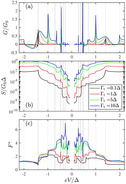
Figure 11: Differential conductance (a), shot noise (b), and Fano factor (c) as a function of the voltage for the case of a single impurity coupled to two superconducting electrodes and for different values of the tunneling rate $\Gamma_{\rm t}$, as indicated in the legend of panel (b). The parameters used are $\Gamma_{\mathrm{S}}=100\Delta,\ J=80\Delta,\ U=60\Delta,\eta_{\rm S}=0.001\Delta,\eta_{\rm t}=0.001\Delta$ and $T=0$. The vertical lines follow the same convention as in Fig. 9.

Figure 12: Charge-resolved currents as a function of the voltage for the cases considered in Fig. 11. Every panel corresponds to a given value of the tip tunneling rate: (a) $\Gamma_{\rm t}=0.1\Delta$, (b) $\Gamma_{\rm t}=\Delta$, (c) $\Gamma_{\rm t}=5\Delta$, and (a) $\Gamma_{\rm t}=10\Delta$. Notice that the absolute value of the current is plotted for clarity. The vertical lines follow the same convention as in Fig. 9.

Again, we can pinpoint the origin of every feature in the transport characteristics by considering the charge-resolved currents, as we illustrate in Fig. 12 (see Fig. S8 for the corresponding charge-resolved conductances [71]). Notice that for the smallest coupling $\Gamma_{\mathrm{t}}=0.1\Delta$ in panel (a) the single-quasiparticle tunneling and the lowest-order Andreev reflection dominate the transport and give similar contributions at $eV=\pm(\Delta+\epsilon_{\mathrm{YSR}})$. However, as the transmission increases, the quasiparticle tunneling becomes progressively more irrelevant in the subgap transport. Thus, for instance, for $\Gamma_{\mathrm{t}}=\Delta$, the structure at $eV=\pm(\Delta+\epsilon_{\mathrm{YSR}})$ is solely due to the resonant Andreev reflection. For $\Gamma_{\mathrm{t}}=5\Delta$ in panel (c), the subgap structure becomes much more pronounced with current steps not only at the standard MAR onsets $eV=\pm 2\Delta/n$, but also at voltages $eV=\pm(\Delta+\epsilon_{\mathrm{YSR}})/2$ and $eV=\pm(\Delta+\epsilon_{\mathrm{YSR}})/3$ which, as explained above, are due to resonant MARs and to YSR-mediated Andreev reflections, respectively. Thus, for instance, the structure at $eV=\pm(\Delta+\epsilon_{\mathrm{YSR}})/2$ is mainly due to the third-order MAR, whereas several YSR-mediated MARs contribute to the structure at $eV=\pm(\Delta+\epsilon_{\mathrm{YSR}})/3$. The steps in the charge-resolved currents are smoothed out when $\Gamma_{\mathrm{t}}$ is further increased towards $\Gamma_{\mathrm{t}}=10\Delta$ in panel (d). In this case the first YSR resonance becomes so broad that it can barely be identified as a resonance, whereas the higher-order YSR resonances are still very sharp and become increasingly easy to detect.

To conclude this section, let us say that one can provide some analytical insight in the tunnel regime when $\Gamma_{\mathrm{t}}\ll\Gamma_{\mathrm{S}}$. In this limit, and with the help of Ref. [62], one can derive perturbative expressions for the current contributions of single-quasiparticle tunneling ($I_{1}$) and the lowest-order Andreev reflection ($I_{2}$). These expressions are given by

$$I^{\rm tunnel}_{1}(V) \approx \frac{4e\pi^{2}}{h}\Gamma_{\mathrm{t}}\int^{\infty}_{-\infty}\rho_{\rm t}(E-eV)\rho_{\mathrm{imp}}(E)\times$$ (81)

$$\left[f(E-eV)-f(E)\right]dE,$$

$$I^{\rm tunnel}_{2}(V) \approx \frac{8e\pi^{2}}{h}\Gamma_{\mathrm{t}}^{2}\int^{\infty}_{-\infty}\rho_{\rm t}(E-eV)\rho_{\rm t}(E+eV)\times$$ (82)

$$|F(E)|^{2}\left[f(E-eV)-f(E+eV)\right]dE.$$

Here, $\rho_{\rm t}(E)$ is the BCS DOS of the superconducting tip, $\rho_{\mathrm{imp}}(E)$ is the total DOS of the impurity coupled to the superconducting substrate, and $F(E)$ is the corresponding anomalous Green’s function of the impurity coupled to the substrate. The impurity DOS is given by

$$\rho_{\mathrm{imp}}(E) = \frac{1}{\pi}\Im\left[\frac{E\Gamma_{\rm S}+(U+E-J)\sqrt{\Delta^{2}-E^{2}}}{D(E)}+\right.$$ (83)

$$\left.\frac{-E\Gamma_{\rm S}+(U-E-J)\sqrt{\Delta^{2}-E^{2}}}{D(-E)}\right],$$

where

$$D(E) = 2\Gamma_{\rm S}E(E-J)+$$ (84)

$$\left[(E-J)^{2}-U^{2}-\Gamma_{\rm S}^{2}\right]\sqrt{\Delta^{2}-E^{2}},$$

and the impurity anomalous Green’s function is given by

$$F(E)=\frac{\Gamma_{\rm S}\Delta}{D(E)}.$$ (85)

By construction, these perturbative current formulas are only valid in the tunnel regime, but they also require the broadening of the YSR states to be large in comparison with the tip tunneling rate $\Gamma_{\rm t}$. To test these approximate formulas, we present in Fig. 13 a comparison with the exact numerical results for the case in which $\Gamma_{\mathrm{S}}=100\Delta$, $J=80\Delta$, $U=60\Delta$, $\eta_{\rm t,S}=0.01\Delta$, $\Gamma_{\mathrm{t}}=0.01\Delta$, and $T=0$. Notice that the analytical formulas nicely reproduce the numerical results, except for the Andreev reflection contribution at very low bias when higher-order terms in the transmission are expected to play a role.

Figure 13: Comparison between the analytical results of Eqs. (81) and (82) for the current contributions from single-quasiparticle tunneling and Andreev reflection and the numerically exact results obtained from the CGF. The different parameters of the model are: $\Gamma_{\mathrm{S}}=100\Delta$, $J=80\Delta$, $U=60\Delta$, $\eta_{\rm t/S}=0.01\Delta$, $\Gamma_{\mathrm{t}}=0.01\Delta$, and $T=0$.

VIII Double-impurity junctions: Tunneling between YSR states

As mentioned in Sec. I, recently it has been experimentally demonstrated that a superconducting STM tip can be functionalized with a magnetic impurity that then features YSR states [25]. More importantly, it was shown that this YSR-STM can be used to probe other magnetic impurities deposited on a superconducting substrate that also features YSR states. In this way, these experiments realized for the first time the tunneling between individual superconducting bound states at the atomic scale, which is the ultimate limit for quantum transport. In particular, the current-voltage characteristics in these double-impurity junctions were shown to exhibit huge current peaks inside the gap (with an extremely pronounced negative differential conductance). These current peaks have been interpreted as the evidence of tunneling between YSR states (both direct at low temperatures and thermally excited at high temperatures) [25, 73, 26]. In this section we want to analyze this unique situation from the FCS point of view and, in particular, provide very concrete predictions for the shot noise and Fano factor in these junctions. In turn, this problem gives us the opportunity to show how the FCS approach can be used in a case in which the scattering matrix is not diagonal in spin space.

VIII.1 Model and scattering matrix

In the spirit of the Keldysh action of Eq. (9) we now need a scattering matrix describing these double impurity junctions. For this purpose, we follow the model put forward in Ref. [73], which has been very successful describing the experimental observations for the current-voltage characteristics [25, 26]. We briefly describe this model and then proceed to the determination of the corresponding normal-state scattering matrix.

Figure 14: Schematic representation of our two-impurity model. Two magnetic impurities are respectively coupled to a superconducting substrate and to an STM tip that is also superconducting. The tunneling rates $\Gamma_{\rm t}$ and $\Gamma_{\rm S}$ measure the strength of the coupling of the impurity to the tip and substrate, respectively, and $v$ is the hopping matrix element describing the tunnel coupling between the impurities. These impurities have magnetizations $\bm{J}_{\mathrm{t}}$ and $\bm{J}_{\mathrm{S}}$ whose relative orientation is described by the angle $\theta$.

The double-impurity model of Ref. [73] is schematically illustrated in Fig. 14. In this model, and inspired by the experiments of Ref. [25], every impurity is strongly coupled to a given superconducting lead (tip and substrate) and both impurities are coupled via a tunnel coupling. The Hamiltonian describing this model is given by [73]

$$H = H_{\mathrm{lead,t}}+H_{\mathrm{imp,t}}+H_{\mathrm{hopping,t}}+$$ (86)

$$H_{\mathrm{lead,S}}+H_{\mathrm{imp,S}}+H_{\mathrm{hopping,S}}+V,$$

where $H_{\mathrm{lead},j}$ describes the Hamiltonian of lead $j={\rm t,S}$, $H_{\mathrm{imp},j}$ describes the respective impurity which is coupled to lead $j$ via the Hamiltonian $H_{\mathrm{hopping,j}}$ and $V$ describes the coupling between the two impurities. We choose a global $z$-quantization axis in which to describe the creation and annihilation operators

$$\bar{c}_{\bm{k},j}^{\dagger} =\left(c_{\bm{k}\uparrow,j}^{\dagger},c_{-\bm{k}\downarrow,j},c_{\bm{k}\downarrow,j}^{\dagger},-c_{-\bm{k}\uparrow,j}\right)$$ (87)

$$\bar{d}^{\dagger}_{j} =\left(d_{\uparrow,j}^{\dagger},d_{\downarrow,j},d_{\downarrow,j}^{\dagger},-d_{\uparrow,j}\right),$$ (88)

where $\bar{c}_{\bm{k},j}^{\dagger}$ corresponds to lead $j$ and $\bar{d}^{\dagger}_{j}$ to impurity $j$. We can express the different terms of the Hamiltonian in their respective basis as follows

$$H_{\mathrm{lead},j} =\frac{1}{2}\sum_{\bm{k}}\bar{c}_{\bm{k},j}^{\dagger}\bar{H}_{\bm{k},j}\bar{c}_{\bm{k},j}$$ (89)

$$H_{\mathrm{imp},j} =\frac{1}{2}\bar{d}_{j}^{\dagger}\bar{H}_{\mathrm{imp}}\bar{d}_{j}$$ (90)

$$H_{\mathrm{hopping},j} =\frac{1}{2}\sum_{\bm{k}}\left(\bar{c}_{\bm{k},j}^{\dagger}\bar{V}_{j}\bar{d}_{j}+\bar{d}_{j}^{\dagger}\bar{V}_{j}^{\dagger}\bar{c}_{\bm{k},j}\right),$$ (91)

where the respective matrices in spin-Nambu space take the form

$$\bar{H}_{\bm{k},j} =\sigma_{0}\otimes\left(\xi_{\bm{k},j}\tau_{3}+\Delta_{j}e^{\imath\varphi_{j}\tau_{3}}\tau_{1}\right)$$ (92)

$$\bar{H}_{\mathrm{imp},j} =U_{j}\sigma_{0}\otimes\tau_{3}+\bm{J}_{j}\cdot(\bm{\sigma}\otimes\tau_{0})$$ (93)

$$\bar{V}_{j} =t_{j}\sigma_{0}\otimes\tau_{3},$$ (94)

with the on-site energies $U_{j}$ and the exchange energies $\bm{J}_{j}$. The tunneling term between the two magnetic impurities reads

$$V=\frac{1}{2}\bar{d}^{\dagger}_{\mathrm{t}}\bar{V}_{\mathrm{tS}}\bar{d}_{\mathrm{S}}+\frac{1}{2}\bar{d}^{\dagger}_{\mathrm{S}}\bar{V}_{\mathrm{St}}\bar{d}_{\mathrm{t}},$$ (95)

with the coupling matrix

$$\bar{V}_{\mathrm{St}}=v(\sigma_{0}\otimes\tau_{3})=\bar{V}_{\mathrm{tS}}^{\dagger},$$ (96)

where $v$ is the tunneling coupling between the impurities. To simplify things, it is convenient to transfer the dependence on $\theta_{j}$ and $\varphi_{j}$ to the coupling term $V$ in Eq. (86) and work with Hamiltonians describing the subsystems in which the corresponding spin points along its quantization axis. For this purpose, we introduce the combined unitary transformation $\bar{R}_{j}=e^{\imath\theta_{j}\sigma_{2}/2}\otimes e^{-\imath\varphi_{j}\tau_{3}/2}$, where $\theta_{j}$ is the angle formed between the exchange energy $\bm{J}_{j}$ and the global $z$-quantization axis. Upon performing this unitary transformation, the Hamiltonian matrices of Eqs. (92)-(94) become now

$$\bar{\mathcal{H}}_{\bm{k},j} =\sigma_{0}\otimes\left(\xi_{\bm{k},j}\tau_{3}+\Delta_{j}\tau_{1}\right)$$ (97)

$$\bar{\mathcal{H}}_{\mathrm{imp},j} =U_{j}\sigma_{0}\otimes\tau_{3}+J_{j}(\sigma_{3}\otimes\tau_{0})$$ (98)

$$\bar{\mathcal{V}}_{j} =t_{j}\sigma_{0}\otimes\tau_{3},$$ (99)

while the coupling matrices in Eq. (96) adopt now the form

$$\bar{\mathcal{V}}_{\mathrm{tS}} =v\left(e^{-\imath\theta\sigma_{2}/2}\otimes\tau_{3}e^{-\imath\varphi_{0}\tau_{3}/2}\right)$$ (100)

$$\bar{\mathcal{V}}_{\mathrm{St}} =v\left(e^{\imath\theta\sigma_{2}/2}\otimes\tau_{3}e^{\imath\varphi_{0}\tau_{3}/2}\right).$$ (101)

Notice that these coupling matrices effectively describe a spin-active interface in which there are spin-flip processes whose probabilities depend on the relative orientation of the impurity spins described by $\theta$.

To obtain the scattering matrix, we shall make use again of the Fischer-Lee relations. For this purpose, we first notice that the central region is now twice as big as in the single-impurity case, and the corresponding Hamiltonian describing this region reads

$$\mathcal{H}_{\mathrm{C}}=\begin{pmatrix}\bar{\mathcal{H}}_{\mathrm{imp,t}}&\bar{\mathcal{V}}_{\mathrm{tS}}\\ \bar{\mathcal{V}}_{\mathrm{St}}&\bar{\mathcal{H}}_{\mathrm{imp,S}}\end{pmatrix}$$ (102)

in the rotated basis $(\mathcal{d}_{\mathrm{t}}^{\dagger},\mathcal{d}_{\mathrm{S}}^{\dagger})\equiv(\bar{R}_{\mathrm{t}}\bar{d}_{\mathrm{t}}^{\dagger},\bar{R}_{\mathrm{S}}\bar{d}_{\mathrm{S}}^{\dagger})$. As in previous cases, only the electron-components of the matrix representation are needed for the computation of the scattering matrix, namely the first and third component of the spinor basis in Eq. (88). Explicitly, that part of the Hamiltonian of the central system reads

$$\mathcal{H}_{\mathrm{C},e}=\begin{pmatrix}U_{\mathrm{t}}+eV+J_{\mathrm{t}}&0&v\cos(\theta/2)&-v\sin(\theta/2)\\ 0&U_{\mathrm{t}}+eV-J_{\mathrm{t}}&v\sin(\theta/2)&v\cos(\theta/2)\\ v\cos(\theta/2)&v\sin(\theta/2)&U_{\mathrm{S}}+J_{\mathrm{S}}&0\\ -v\sin(\theta/2)&v\cos(\theta/2)&0&U_{\mathrm{S}}-J_{\mathrm{S}},\end{pmatrix}$$ (103)

in the basis $(\mathcal{d}_{\uparrow,\mathrm{t}}^{\dagger},\mathcal{d}_{\downarrow,\mathrm{t}}^{\dagger},\mathcal{d}_{\uparrow,\mathrm{S}}^{\dagger},\mathcal{d}_{\downarrow,\mathrm{S}}^{\dagger})$. Notice that we have included the bias voltage $V$ in the tip subsystem as a shift of the corresponding impurity level. This way we describe a situation in which the voltage entirely drops between the two impurities, as it happens in the STM experiments. On the other hand, the couplings can be expressed as $H_{\mathrm{hopping},j}=\frac{1}{2}\sum_{\bm{k}}(\mathcal{c}_{\bm{k}\uparrow,\mathrm{j}}^{\dagger},\mathcal{c}_{\bm{k}\downarrow,\mathrm{j}}^{\dagger})\mathcal{V}_{j,\rm e}(\mathcal{d}_{\uparrow,\mathrm{t}},\mathcal{d}_{\downarrow,\mathrm{t}},\mathcal{d}_{\uparrow,\mathrm{S}},\mathcal{d}_{\downarrow,\mathrm{S}})^{\rm T}+\mathrm{c.c.}$, where the matrices $\mathcal{V}_{j,\rm e}$ are given by

$$\mathcal{V}_{\mathrm{t},e} =\begin{pmatrix}t_{\mathrm{t}}&0&0&0\\ 0&t_{\mathrm{t}}&0&0\end{pmatrix}$$ (104)

$$\mathcal{V}_{\mathrm{S},e} =\begin{pmatrix}0&0&t_{\mathrm{S}}&0\\ 0&0&0&t_{\mathrm{S}}\end{pmatrix}.$$ (105)

With these couplings, the self-energies of the tip and substrate can be readily computed as we are only interested in the normal state scattering matrix, and thus the lead GFs are normal metal ones. In particular, the (normal-state) electron part of the GFs are given by $g_{\mathrm{N,e}}^{\rm r/a}=\mp\imath\sigma_{0}$. Thus, the self-energies read

$$\Sigma_{\rm t,e}^{\rm r/a} =\mathcal{V}_{\mathrm{t,e}}^{\dagger}g^{\rm r/a}_{\mathrm{N,e}}\mathcal{V}_{\mathrm{t,e}}$$ (106)

$$\Sigma_{\rm S,e}^{\rm r/a} =\mathcal{V}_{\mathrm{S,e}}^{\dagger}g^{\rm r/a}_{\mathrm{N,e}}\mathcal{V}_{\mathrm{S,e}},$$ (107)

or more explicitly

$$\Sigma_{\rm t,e}^{\rm r/a}=\mp\imath\begin{pmatrix}\Gamma_{\rm t}&0&0&0\\ 0&\Gamma_{\rm t}&0&0\\ 0&0&0&0\\ 0&0&0&0\end{pmatrix}$$ (108)

$$\Sigma_{\rm S,e}^{\rm r/a}=\mp\imath\begin{pmatrix}0&0&0&0\\ 0&0&0&0\\ 0&0&\Gamma_{\rm S}&0\\ 0&0&0&\Gamma_{\rm S}\end{pmatrix},$$ (109)

so they are $4\times 4$ matrices in impurity-spin space and they are not of full rank. The dressed central GFs can then be computed from the Dyson equation

$$G_{\mathrm{C},e}^{\mathrm{r/a}}=\left[(E\pm\imath\eta_{\mathrm{imp}})1-\mathcal{H}_{\mathrm{C},e}-\Sigma_{\rm t,e}^{\rm r/a}-\Sigma_{\rm S,e}^{\rm r/a}\right]^{-1},$$ (110)

with the regularization factor $\eta_{\mathrm{imp}}$ which can again be chosen as zero, as in the single impurity case. To compute the components, we also need the scattering rate matrices $\bm{\Gamma}_{\rm t}\equiv\Im(\Sigma_{\mathrm{t,e}}^{\rm a})$ and $\bm{\Gamma}_{\rm S}\equiv\Im(\Sigma_{\mathrm{S,e}}^{\rm a})$. Finally, the scattering matrix then follows from the Fisher-Lee relation using the $4\times 4$ dressed central GFs, namely

$$s_{\rm e}(E,V) =\begin{pmatrix}\mathfrak{r}_{\rm{e}}&\mathfrak{t}_{\rm{e}}^{\prime}\\ \mathfrak{t}_{\rm{e}}&\mathfrak{r}_{\rm{e}}^{\prime}\end{pmatrix}$$ (111)

$$=\rho_{3}\sigma_{0}-2\imath\left(\bm{\Gamma}_{\rm t}^{1/2}+\imath\bm{\Gamma}_{\rm S}^{1/2}\right)G_{\rm C,e}^{\rm r}\left(\bm{\Gamma}_{\rm t}^{1/2}+\imath\bm{\Gamma}_{\rm S}^{1/2}\right),$$

where $\rho_{3}$ is the third Pauli matrix in lead space. For the hole part of the scattering matrix, it holds that

$$s_{\rm h}(E,V)=\sigma_{2}s_{\rm e}(-E,V)^{\rm T}\sigma_{2},$$ (112)

and the total scattering matrix reads

$$s(E,V)=\mathrm{diag}(s_{\rm e}(E,V),s_{\rm h}(E,V)).$$ (113)

VIII.2 Results

The calculation of the Keldysh action in this double-impurity case is very similar to that of a single impurity discussed in Sec. VII. Again, we have to treat the problem in the Floquet language and resort to numerics to compute the charge-resolved probabilities. On a conceptual level, the main differences are that the scattering matrix has a different energy dependence and it is non-diagonal in spin space. Therefore, it can be shown that the CGF in this case reads

$$\mathcal{A}_{t_{0}}(\chi)=\frac{t_{0}}{2h}\int^{eV}_{-eV}dE\ln\left[\sum_{n=-\infty}^{\infty}P_{n}(E,V)e^{\imath n\chi}\right],$$ (114)

where $P_{n}(E,V)$ corresponds to the probability of transferring $n$ charges across the junction and $E$ is the Floquet energy. Notice the absence of the spin index, when compared to Eq. (78). We can then compute the current and the noise, which are given by the standard formulas of a multinomial distribution

$$I(V) = \frac{e}{2h}\int^{eV}_{-eV}dE\sum^{\infty}_{n=-\infty}nP_{n}(E,V),$$ (115)

$$S(V) = \frac{e^{2}}{h}\int^{eV}_{-eV}dE\left\{\sum^{\infty}_{n=-\infty}n^{2}P_{n}(E,V)-\right.$$

$$\hskip 79.6678pt\left.\left(\sum^{\infty}_{n=-\infty}nP_{n}(E,V)\right)^{2}\right\}.$$

Figure 15: Zero-temperature current (a), shot noise (b), and Fano factor (c) as a function of the voltage for the case of two impurities coupled to their respective superconducting electrodes at zero temperature. The two superconductors are assumed to be identical and have a gap equal to $\Delta$. The model parameters used in this example are: $\Gamma_{\rm t}=\Gamma_{\rm S}=100\Delta$, $J_{\rm t}=60\Delta$, $U_{\rm t}=0$, $J_{\rm S}=60\Delta$, $U_{\rm S}=60\Delta$, $\eta_{\rm t}=\eta_{\rm S}=0.001\Delta$, $v=\Delta$, and $\theta=\pi/2$. With these parameters the junction has a normal state conductance of $4\times 10^{-4}G_{0}$ and the YSR energies are $\epsilon_{\rm t}=0.48\Delta$ and $\epsilon_{\rm S}=0.64\Delta$. In the different panels, the black lines correspond to the exact results (including all possible contributions) and the red lines to the contribution of single-quasiparticle tunneling. The dotted vertical lines indicate the position of the voltages $eV=\pm|\epsilon_{\rm S}+\epsilon_{\rm t}|$ of the direct Shiba-Shiba tunneling. (d-f) The same as in panels (a-c), but for a temperature $k_{\rm B}T=0.2\Delta$ with additional dotted vertical lines indicating the position of the voltages $eV=\pm|\epsilon_{\rm S}-\epsilon_{\rm t}|$ of the thermal Shiba-Shiba tunneling. (g,h) Schematic representation of the tunneling processes between the two YSR states. Here, the left electrode is a magnetic impurity coupled to a SC tip and the right one is another impurity coupled to a superconducting substrate both featuring YSR states. The green shaded areas represent the corresponding Fermi functions of both electrodes. The diagrams follow the same convention as in Fig. 2. Panel (g) corresponds to the direct Shiba-Shiba tunneling enabled by a finite spin-mixing angle $\theta$ and panel (h) to the thermal Shiba-Shiba tunneling enabled by a finite temperature and a spin-mixing angle $\theta\neq\pi$.

To make a connection with the experiments of Refs. [25, 26], we shall mainly focus here on the analysis of the results in the regime of weak coupling between the impurities in which the transport properties are mainly determined by the tunneling of quasiparticles. Moreover, we shall assume that the two superconducting electrodes are identical and the corresponding gap is given by $\Delta$. To illustrate the results in the weak-coupling regime, we consider an example in which the different model parameters are given by: $\Gamma_{\rm S,t}=100\Delta$, $J_{\rm t}=60\Delta$, $U_{\rm t}=0$, $J_{\rm S}=60\Delta$, $U_{\rm S}=60\Delta$. With these parameters, the YSR energies are $\epsilon_{\rm t}=0.48\Delta$ for the SC tip and $\epsilon_{\rm S}=0.64\Delta$ for the substrate. The Dynes’ parameter is chosen to be the same for both SCs $\eta_{\rm t,S}=0.001\Delta$. Moreover, we choose the impurity coupling $v=\Delta$ such that the normal state conductance is relatively low ($\approx 4\times 10^{-4}G_{0}$) and the quasiparticle tunneling dominates the transport. Finally, the spin-mixing angle is chosen as $\theta=\pi/2$, which has been shown to reproduce the experimental results [26]. Actually, this value was interpreted as a way to describe the average transport properties in a situation in which the two spins are freely rotating, see Ref. [26] for details. The results for the current, shot noise, and Fano factor as a function of the bias voltage are shown in Fig. 15 for two cases: zero temperature ($k_{\rm B}T=0$) and $k_{\rm B}T=0.2\Delta$. Let us first discuss the zero-temperature results. The main salient feature in the current is the appearance of very pronounced peaks (with a huge negative differential conductance) inside the gap region at voltages given by $eV=\pm|\epsilon_{\rm S}+\epsilon_{\rm t}|\approx\pm 1.12\Delta$, see Fig. 15(a), which reproduces the main observation in Refs. [25, 26]. As explained in Refs. [25, 73, 26], these current peaks are due to the resonant quasiparticle tunneling between the lower and upper YSR states of the impurities in the tip and substrate, as we illustrate in Fig. 15(g). Such a tunneling process, which we shall refer to as direct Shiba-Shiba tunneling, can occur at any temperature and it only requires the impurity spins to be nonparallel (i.e., $\theta\neq 0$), otherwise it would be forbidden due to the full spin polarization of the YSR states. Notice that in Fig. 15(a) we compare the exact result taking into account any possible contribution (also from Andreev reflections) and the result only including single-quasiparticle tunneling ($n=\pm 1$). Such a comparison shows that the current is dominated in this case by quasiparticle tunneling. With respect to the shot noise, see Fig. 15(b), it exhibits the same voltage dependence as the current and it shows two pronounced peaks at $eV=\pm|\epsilon_{\rm S}+\epsilon_{\rm t}|$ as a result of the direct Shiba-Shiba tunneling. Again, the noise is dominated by the contribution of single-quasiparticle tunneling. Turning now to the Fano factor, see Fig. 15(c), the main feature is the strong reduction at the voltages of the direct Shiba-Shiba tunneling. In this particular case, the Fano factor reaches a value around $0.5$ that actually depends on the bias polarity. Notice that the Fano factor reduction is also dominated by single-quasiparticle tunneling. Obviously, the origin of this pronounced reduction of the Fano factor must be due to the resonant character of this tunneling process between the two individual YSR states. This will be explained below. Notice, on the other hand, that the Fano factor is close to 1 away from the resonant voltage and it reaches values above 1 inside the gap due to the contribution of Andreev reflections.

Turning now to the high temperature case ($k_{\rm B}T=0.2\Delta$), the main novelty in the current is the presence of two additional current peaks inside the gap that appear at $eV=\pm|\epsilon_{\rm t}-\epsilon_{\rm S}|\approx 0.16\Delta$, see Fig. 15(d). These current peaks, which were in fact experimentally observed [25, 26], are due to the thermally activated tunneling between the two upper (or excited) YSR states, as we illustrate in Fig. 15(h). As explained in Refs. [25, 73, 26], this thermally activated tunneling process, which we shall refer to as thermal Shiba-Shiba tunneling, can occur when the temperature is high enough to have a partial occupation of the excited YSR states and it requires that the impurity spins are not antiparallel (i.e., $\theta\neq\pi$), otherwise it would be forbidden due to the full spin polarization of the YSR states. Again, we note that the current in this case is also dominated by single-quasiparticle tunneling, see Fig. 15(d). The thermal Shiba-Shiba tunneling is also visible in the shot noise in the form of two peaks at $eV=\pm|\epsilon_{\rm t}-\epsilon_{\rm S}|$. In the case of the Fano factor, the values at the voltages $eV=\pm|\epsilon_{\rm t}+\epsilon_{\rm S}|$ associated to direct Shiba-Shiba tunneling have increased as compared to the zero-temperature case, while there is no visible feature at the biases of the thermal Shiba-Shiba tunneling because in this example it is masked by the rapid increase of the thermal noise that dominates the low-bias regime in the Fano factor at finite temperatures.

Figure 16: (a) Zero-temperature current and shot noise at the direct Shiba-Shiba energy $eV=|\epsilon_{\rm S}+\epsilon_{\rm t}|$ as a function of the coupling $v$. The rest of the parameters of the model correspond to those of Fig. 15. The solid lines correspond to the exact results, while the dotted lines were computed taking only into account the contribution of the tunneling of single quasiparticles. (b) The corresponding Fano factor $F^{\ast}$. The black line corresponds to the exact results and the red line to the contribution of single-quasiparticle tunneling.

From the discussion of the example of Fig. 15 it is obvious that the most important feature related to the tunneling between two YSR states is the Fano factor reduction at the resonant bias of the direct Shiba-Shiba tunneling. To understand its origin and magnitude we first need to analyze more systematically how this reduction depends on the different parameters of the model. In particular, the Fano factor related to the direct Shiba-Shiba tunneling is expected to depend on the relative value between the effective tunneling rate (related to the hopping element $v$) and the broadening (or lifetime) of the bound states. In fact, this issue is very much related to another interesting observation reported in Ref. [25], namely the fact that the height of the direct Shiba-Shiba current peaks (and their area) undergoes a crossover between a linear regime at very low transmission (or normal state conductance) and a sublinear regime at higher transmission when the STM tip with its impurity was brought closer to the impurity on the substrate. To understand the impact of the junction transmission, we considered the zero-temperature example of Fig. 15 and computed the value of the current, noise and Fano factor at the direct Shiba-Shiba voltage $eV=|\epsilon_{\rm S}+\epsilon_{\rm t}|$ as a function of the hopping matrix element $v$ describing the coupling between the impurities, while the rest of the parameters are kept constant. The results are displayed in Fig. 16, where we show both the exact results and those computed taking only into account the contribution of single-quasiparticle processes. As it can be seen in panel (a), the peak height indeed exhibits the type of crossover observed experimentally. For small values of $v$, i.e., deep into the tunnel regime, the current peak height increases linearly with the transmission (which in this regime is proportional to $v^{2}$) and it crosses over to a sublinear regime at higher couplings. Moreover, this crossover is mainly about the quasiparticle current and only at high enough couplings ($v\gtrsim\Delta$) we start to see additional contributions due to Andreev reflections. Interestingly, the shot noise exhibits a similar crossover, but with an important difference, namely the fact that it enters the sublinear regime more quickly than the current and even exhibits a local minimum at a certain value of $v$. This peculiar behavior is clearly reflected in the evolution of Fano factor, see Fig. 16(b). The Fano factor for very small couplings is equal to 1, as expected from standard (non-resonant) tunneling, it is progressively reduced as the coupling increases reaching a minimum value of around ($\sim 0.22$), and it increases again monotonically for even higher couplings. Notice also that the quasiparticle contribution dominates the Fano factor up to coupling values clearly beyond that at which the minimum takes place.

To understand the origin of this crossover, the existence and magnitude of the Fano factor minimum, and whether this behavior is universal, we put forward the following toy model. We consider two energy levels $\epsilon_{\rm t}$ and $\epsilon_{\rm S}$ that are coupled to their respective electron reservoirs. Due to this coupling, the quantum levels acquire a broadening, which we assume to be equal for both levels and given by $\eta_{\rm S}=\eta_{\rm t}=\eta$. Additionally, these two levels are coupled via a tunnel coupling $v_{\rm eff}$. This model is illustrated in Fig. 17(a). Notice that we do not even need to invoke the existence of superconductivity. The energy and bias dependent electron transmission in this toy model is given by [63]

$$T(E,V)=\frac{4\pi^{2}v_{\rm eff}^{2}\rho_{\rm t}(E-eV)\rho_{\rm S}(E)}{|1-v_{\rm eff}^{2}g_{\rm t}(E-eV)g_{\rm S}(E)|^{2}},$$ (117)

where $g_{\rm t,S}(E)$ are advanced GFs related to both energy levels and given by

$$g_{\rm t,S}(E)=\frac{1}{E-\epsilon_{\rm t,S}-\imath\eta},$$ (118)

and $\rho_{\rm t/S}(E)=(1/\pi)\Im(g_{\rm L/R})$ are the DOS associated to those two levels. Without loss of generality, we choose $\epsilon_{\rm t}<0$, $\epsilon_{\rm S}>0$, and a positive bias. Since we want to emulate the transport properties at the direct Shiba-Shiba energy, we shall set from now on $eV=|\epsilon_{\rm t}|+|\epsilon_{\rm S}|$. At this bias, the transmission adopts the form

$$T(E) =\frac{4v_{\rm eff}^{2}\eta^{2}}{[(E-\epsilon_{\rm S}-v_{\rm eff})^{2}+\eta^{2}][(E-\epsilon_{\rm S}+v_{\rm eff})^{2}+\eta^{2}]}$$

$$=\frac{4\gamma^{2}}{\left[\left(\frac{E-\epsilon_{\rm S}}{\eta}-\gamma\right)^{2}+1\right]\left[\left(\frac{E-\epsilon_{\rm S}}{\eta}+\gamma\right)^{2}+1\right]},$$ (119)

where $\gamma=v_{\rm eff}/\eta$. Within this model, the corresponding zero-temperature current and noise are given by

$$I = \frac{2e}{h}\int_{0}^{eV}T(E)\,dE,$$ (120)

$$S = \frac{4e^{2}}{h}\int_{0}^{eV}T(E)\left[1-T(E)\right]dE.$$ (121)

Assuming that $\eta\ll|\epsilon_{\rm t,S}|$ and $v_{\rm eff}<|\epsilon_{\rm t}|+|\epsilon_{\rm S}|$, one can compute analytically the previous integrals to obtain

$$I = \left(\frac{2e}{h}\right)2\pi\eta\frac{\gamma^{2}}{\gamma^{2}+1},$$ (122)

$$S = \left(\frac{4e^{2}}{h}\right)2\pi\eta\left[\frac{\gamma^{2}}{\gamma^{2}+1}-\frac{\gamma^{4}(\gamma^{2}+5)}{2(\gamma^{2}+1)^{3}}\right].$$ (123)

The corresponding Fano factor is then given by

$$F^{*}=\frac{S}{2eI}=\frac{\gamma^{4}-\gamma^{2}+2}{2(\gamma^{2}+1)^{2}}.$$ (124)

These expressions nicely summarize the type of crossover that we discussed above and show that it is simply controlled by the parameter $\gamma$, i.e., ratio between the tunnel coupling and the level width. Before comparing with the actual results of the two impurity system, let us analyze the Fano factor in different limiting cases. First, in the weak coupling regime $\gamma\ll 1$, the Fano factor becomes 1, which is the expected result for non-resonant tunneling situations. Second, in the high coupling regime $\gamma\gg 1$, the Fano factor tends to $1/2$, which is the generic expected result for two very narrow energy levels. We shall see that this regime cannot be easily achieved with the YSR states because for very large $v$ the Fano factor is altered by the Andreev reflections. More interestingly, the Fano factor can be much smaller than $1/2$. Thus, for instance, for $\gamma=1$ the Fano factor is exactly $1/4$. In particular, the shot noise exhibits a local minimum at this value of $\gamma$, which we propose as a new method to extract the intrinsic lifetime of the states. However, the Fano factor of $1/4$ does not mark the lowest Fano factor. It is easy to show that the minimum Fano factor value is achieved when $\gamma=\sqrt{5/3}>1$, which results in a Fano factor equal to $7/32$. This is a unique value that, to our knowledge, is not found in any other generic situation.

Figure 17: (a) Schematic representation of the model used to describe the tunneling between two bound states. (b) Zero-temperature current and shot noise computed with the model of panel (a) (dotted lines) as a function of the ratio $v_{\rm eff}/\eta$. The solid lines correspond to the exact results taken from Fig. 16 and using the expression of $v_{\rm eff}$ of Eq. (127). The vertical line indicates the case $v_{\rm eff}=\eta$. (c) The corresponding Fano factor computed with the model (dotted line) and the results of Fig. 16(b) (both exact and single-quasiparticle contributions). The solid horizontal line indicates a Fano factor equal to $7/32$, while the the horizontal dashed line corresponds to the Fano factor equal to $1/4$.

To establish a quantitative comparison between the toy model and the direct tunneling between YSR states, we still need to identify the effective tunneling coupling in the latter situation. In the presence of YSR states the effective coupling must take into account both the spin-mixing angle $\theta$ and the coherent factors that determine the height of the DOS associated to the YSR states. These coherent factors are given in our model by

$$u_{j}^{2} =\frac{2J_{j}\Gamma_{j}^{2}\Delta_{j}}{\left[\Gamma_{j}^{2}+(J_{j}+U_{j})^{2}\right]^{3/2}\left[\Gamma_{j}^{2}+(J_{j}-U_{j})^{2}\right]^{1/2}},$$ (125)

$$v_{j}^{2} =\frac{2J_{j}\Gamma_{j}^{2}\Delta_{j}}{\left[\Gamma_{j}^{2}+(J_{j}-U_{j})^{2}\right]^{3/2}\left[\Gamma_{j}^{2}+(J_{j}+U_{j})^{2}\right]^{1/2}}.$$ (126)

with $j=\rm t,S$. Thus, the effective tunnel coupling $v_{\rm eff}$ describing the direct Shiba-Shiba tunneling can be expressed in terms of the bare $v$ hopping matrix elements as follows

$$v_{\rm eff}=v\sin(\theta/2)\times\begin{cases}u_{\rm t}v_{\rm S}&\mbox{for}\;V>0\\ u_{\rm S}v_{\rm t}&\mbox{for}\;V<0\end{cases}.$$ (127)

Finally, we are in position to establish the desired comparison, which is shown in Fig. 17(b,c). There we present both the analytical results obtained with the toy model for the current, noise, and Fano factor at the resonant bias, as well as the exact results shown in Fig. 16(a,b) where the tunnel coupling has been renormalized according to Eq. (127). The results are presented as a function of the ratio $v_{\rm eff}/\eta$. Notice that the toy model is able to quantitative reproduce the results of our two-impurity model over a broad range of values of that ratio. In particular, the toy model nicely reproduces the crossover in all transport properties up to coupling values in which Andreev reflections start playing a role. Interestingly, we now can see that the local minimum in the shot noise exactly corresponds to the case $v_{\rm eff}=\eta$ when the effective coupling is equal to the broadening of the YSR states. Moreover, the minimum of the Fano factor is shown to reach the value $7/32$ predicted by the toy model, and the Fano factor becomes $1/4$ exactly when the shot noise is locally minimal. On the other hand, notice that the prediction of the toy model of a Fano factor equal to $1/2$ when $v_{\rm eff}\gg\eta$ is not reached in the direct Shiba-Shiba tunneling case due to the onset of the Andreev reflections, as one can see in Fig. 17(c). Finally, the most important conclusion of the impressive agreement with the toy model is the universality of the results when considered as a function of the the ratio $v_{\rm eff}/\eta$, as long as the transport is dominated by the tunneling of single quasiparticles. This universality is illustrated in Ref. [71] where we present the results for this crossover for different sets of values of the model parameters, see Fig. S15.

It is important to stress that our FCS approach is valid for arbitrary junction transparency and can also describe situations in which the transport is dominated by MARs. Actually, this is a very interesting subject since, as it has been theoretically shown in Ref. [73] for the current, the transport properties are expected to exhibit an extremely rich subgap structure due to the occurrence of a variety of different types of MARs, some of which have no analog in the single-impurity case. However, due to the richness of that physics, and to keep the length of this manuscript under control, we shall postpone the analysis of that regime to a forthcoming publication. In any case, we have included some examples of the high transparency regime in Ref. [71] to illustrate once more the power of our FCS approach, see Figs. S10-S14.

IX Discussion and conclusions

As explained in Sec. I, the concept of FCS has already been used to understand the transport properties of several basic superconducting junctions. However, the Keldysh action described in Sec. III [60, 61], which has remained fairly unnoticed, puts this concept at a whole new level because it allows us to describe the coherent transport in situations where the scattering matrix of the system may depend on energy, spin, and even involve an arbitrary number of superconducting terminals. Here, we have shown how this action can be used in practice by combining it with model Hamiltonians, and we have illustrated its power in the several examples concerning the spin-dependent transport in hybrid superconducting systems that exhibit YSR states. Such a combination opens up the possibility to shed new light on the coherent transport in numerous superconducting nanostructures. Thus, for instance, among the natural extensions of this work we can mention the study of Majorana physics in magnetic atomic chains from the FCS point of view [34, 35, 36, 37, 38, 39, 40]. In fact, it has been recently suggested that shot-noise tomography in hybrid magnetic-superconducting wire systems could be used to distinguish Majorana modes from other trivial fermionic states [74]. Another context in which one could straightforwardly apply our FCS approach is that of superconductor-semiconductor nanowire junctions in which one can realize single and double quantum dot systems that exhibit YSR states, see Refs. [75, 76, 77] and references therein. An interesting situation in which it would be very interesting to apply the FCS approach is that of microwave-irradiated junctions [78, 79, 80]. It has been recently shown that one can gain some new insight into the interplay between YSR states and Andreev transport by studying the single-impurity systems discussed in this work with the assistance of a microwave field [81, 82, 83]. Probably the most exciting possibility of the approach put forward in this work is the analysis of multiterminal superconducting systems. As mentioned above, the Keldysh action described here is valid for arbitrary number of terminals. In this sense, we are very much interested in extending this work to study different aspects of superconducting multiterminal systems that are currently attracting a lot of attention such as the generation of Cooper quartets [84, 85, 86, 87, 88], the study of the Josephson effects [89, 90, 91, 92], or the possibility to engineer Andreev bound states with interesting topological properties [93, 94, 95, 96, 97, 98, 99, 100, 101, 102, 103, 104]. Last but not least, nothing prevents us from using this FCS approach in the case of junctions involving unconventional superconductors.

It is worth remarking that our whole analysis of the FCS in these impurity systems has been done making use of mean-field models. In that regard, it would be interesting, albeit very challenging, to investigate the role of electronic correlations or spin fluctuations in the transport properties discussed in this work, most notably in the noise. This clearly goes beyond the scope of this work and it cannot be done with the action of Eq. (9) used here as starting point. The success of these mean-field models is indeed quite remarkable, as we have shown in Sec. VI and has been demonstrated in numerous publications [9, 23, 25, 26, 27, 81, 82, 73, 83]. So, it will be interesting to see if future shot noise experiments reveal the presence of significant correlation effects.

To summarize the present work, let us say that we have shown here that the FCS approach can be extended to describe the spin-dependent transport in systems involving magnetic impurities coupled to superconducting leads. In particular, with the analysis of different situations we have illustrated how the concept of FCS provides an unprecedented insight into the interplay between YSR states and electronic transport. Among the lessons and predictions put forward here, we can highlight the following ones. First, in the case of single-impurity junctions with only one superconducting electrode, we have shown that the whole subgap transport can be understood as a competition between single-quasiparticle tunneling and a resonant Andreev reflection. Such a competition is especially reflected in the shot noise and Fano factor, which allow us to access energy scales that are out of the scope of conventional conductance measurements, most notably the YSR lifetimes. In particular, we have illustrated this fact with the analysis of very recent experiments that have reported for the first time shot noise measurements in these hybrid atomic-scale systems [49]. Second, in the case of single-impurity junctions with two superconducting leads, we have shown how the FCS concept allows us to unambiguously identify the contribution of all the tunneling processes, including multiple Andreev reflections. In particular, this has helped us to correct common misinterpretations on the origin of certain features in the subgap structure of the conductance. In particular, we have discussed the unique signatures of the so-called resonant multiple Andreev reflections (multiple versions of the known lowest-order resonant Andreev reflection), which should enable their experimental identification, something that to our knowledge has not been reported thus far. Moreover, we have presented extensive predictions on how the occurrence of these resonant Andreev reflections, and YSR-mediated Andreev reflections, are reflected in the shot noise and Fano factor. Finally, in connection to recent experiments on the tunneling between two individual YSR states in two-impurity systems [25, 26], we have shown that such a tunneling leads to an unambiguous signature in the Fano factor in the form of a strong reduction at the resonant bias voltage at which the two YSR states are aligned. In particular, we have demonstrated that the direct Shiba-Shiba tunneling at low temperatures can exhibit a Fano factor as small as $7/32$, which results from the resonant quasiparticle tunneling between two YSR states. This constitutes a novel result in quantum transport that has not been realized in any other system. So, in short, we think that these examples and predictions will motivate other theoretical groups to use the concept of FCS to provide a new point of view on the superconducting transport in numerous situations. Moreover, our work clearly shows the importance of going beyond conductance measurements to truly understand the Andreev transport in the presence of superconducting bound states. In this sense, we are convinced that this work will trigger off the realization of new shot noise measurements in these atomic-scale superconducting systems exhibiting YSR states.

Appendix A Keldysh Green function formalism

One ingredient for the Keldysh action in Eq. (9) are the Green’s functions (GFs) of the leads, which are described in the framework of the Keldysh formalism [105]. We provide a more in-depth discussion of these functions in this Appendix. The retarded and advanced GFs of a BCS superconductor (SC) in spin-Nambu space are given by

$$\bar{g}^{\rm r/a}(E) =\sigma_{0}\otimes\frac{-\imath}{\sqrt{\Delta^{2}-(E\pm\imath\eta)^{2}}}\begin{pmatrix}(E\pm\imath\eta)&\Delta e^{\imath\phi}\\ -\Delta e^{-\imath\phi}&-(E\pm\imath\eta)\end{pmatrix}$$

$$=\sigma_{0}\otimes\begin{pmatrix}g^{\rm r/a}&f^{\rm r/a}\\ {\mathfrak{f}^{\rm r/a}}&-g^{\rm r/a}\end{pmatrix},$$ (128)

where we have used the spinor basis $(\Psi_{\uparrow}^{\dagger},\Psi_{\downarrow},\Psi_{\downarrow}^{\dagger},-\Psi_{\dagger})$ and the Pauli matrices $\sigma_{i}$ in spin space, $\sigma_{0}$ being the identity. Note that we already eliminated the $k$-dependence by summing it out. The bar ($\ \bar{}\$) indicates that a quantity is expressed in spin-Nambu space. The SC is described by a gap $\Delta>0$ and the phase of the SC condensate $\phi$. The regularization parameter $\eta$ should in principle tend to zero in these expressions, but it can be kept constant to describe in simple terms inelastic mechanisms that tend to broaden the electronic states (Dynes’ parameter). Note that we are using here GFs subjected to the normalization condition $\bar{g}^{\rm r/a}\bar{g}^{\rm r/a}=\bar{1}$, where $\bar{1}$ is the identity in spin-Nambu space. Notice also that the GFs are block-diagonal in spin space

$$\bar{g}^{\rm r/a}(E)=\begin{pmatrix}g^{\rm r/a}_{\Uparrow}(E)&0\\ 0&g^{\rm r/a}_{\Downarrow}(E)\end{pmatrix},$$ (129)

where $g^{\rm r/a}_{\Uparrow}(E)$ is the GF in the spinor basis $\Psi_{\Uparrow}=(\Psi_{\uparrow}^{\dagger},\Psi_{\downarrow})$, including spin-up electrons and spin-down holes, whereas $g^{r/a}_{\Downarrow}(E)$ is the GF in the spinor basis $\Psi_{\Downarrow}=(\Psi_{\downarrow}^{\dagger},-\Psi_{\uparrow})$, describing spin-down electrons and spin-up holes. We shall assume in this work that $g_{\Uparrow}=g_{\Downarrow}$ (no net spin polarization in the electrodes).

In the case of a normal metal ($\Delta=0$), the GFs reduce to

$$\bar{g}^{\rm r/a}_{\mathrm{N}}(E)=\pm\sigma_{0}\otimes\tau_{3},$$ (130)

where we have used the Pauli matrices $\tau_{i}$ in Nambu space.

To deal with nonequilibrium situations, we consider the Keldysh GFs of a SC given by

$$\check{g}(E)=\begin{pmatrix}\bar{g}^{--}&\bar{g}^{-+}\\ \bar{g}^{+-}&\bar{g}^{++}\end{pmatrix}=\frac{1}{2}\begin{pmatrix}\bar{g}^{\rm a}+\bar{g}^{\rm r}+\bar{g}^{\rm k}&\bar{g}^{\rm a}-\bar{g}^{\rm r}+\bar{g}^{\rm k}\\ \bar{g}^{\rm a}-\bar{g}^{\rm r}-\bar{g}^{\rm k}&\bar{g}^{\rm a}+\bar{g}^{\rm r}-\bar{g}^{\rm k}\end{pmatrix},$$ (131)

with the retarded and advanced GF in spin-Nambu basis from Eq. (A) and the Keldysh component of the GF $\bar{g}^{\rm k}=(\bar{g}^{\rm r}-\bar{g}^{\rm a})(1-2f)$ with the Fermi function of the superconductor $f(E)=1/(e^{E/k_{\mathrm{B}}T}+1)$ with the temperature $T$ and the Boltzman constant $k_{\mathrm{B}}$. The index $(\ \check{}\ )$ indicates that the GF is expressed in Keldysh-spin-Nambu space. The Keldysh GF can be brought into the time-domain by a Fourier transformation as follows:

$$\check{g}(t_{\mathrm{rel}})=\int dE\,\check{g}(E)e^{\imath Et_{\mathrm{rel}}},$$ (132)

where $t_{\mathrm{rel}}=t-t^{\prime}$ is the relative time. If a reservoir is voltage biased, the voltage can be gauged onto the GF. Namely, for a constant bias voltage $V$, the SC phase is given by $\phi(t)=2eVt/\hbar$ (where the dc phase $\phi_{0}$ is already included in the GF in Eq. (A)). The voltage dependent GF is then obtained via

$$\check{g}(t,t^{\prime})=e^{\imath\phi(t)(\nu_{0}\otimes\sigma_{0}\otimes\tau_{3})/2}\check{g}(t_{\mathrm{rel}})e^{-\imath\phi(t^{\prime})(\nu_{0}\otimes\sigma_{0}\otimes\tau_{3})/2},$$ (133)

where the Pauli matrices in Keldysh $\nu_{i}$, spin $\sigma_{i}$ and Nambu $\tau_{i}$ space and their respective identities $\nu_{0}$, $\sigma_{0}$ and $\tau_{0}$ are used. Similar to the voltage, the counting field $\chi$ can be gauged onto the SC GF

$$\check{g}(\chi,t,t^{\prime})=e^{-\imath\chi(\nu_{3}\otimes\sigma_{0}\otimes\tau_{3})/2}\check{g}(t,t^{\prime})e^{\imath\chi(\nu_{3}\otimes\sigma_{0}\otimes\tau_{3})/2}.$$ (134)

Since we only consider two-terminal settings in this work, we only need a single counting field (the other one can be gauged away). Additionally, the non-diagonal entries in Nambu space result in a dependence of the GF on the average time $t_{\rm av}=(t+t^{\prime})/2$. We can thus express the GF as a function of relative time $t_{\rm rel}$ and average time $t_{\rm av}=(t+t^{\prime})/2$, namely $\check{g}(t_{\rm rel},t_{\rm av})$. For a normal metal, the off-diagonal entries in Nambu space are zero and the GFs only depend on the relative time $t_{\mathrm{rel}}$. Then, the GFs can be trivially Fourier transformed back with respect to $t_{\mathrm{rel}}$ to the energy space. However, because of the occurrence of $t_{\mathrm{av}}$, this is not possible in the SC case. Hence, we introduce the Wigner representation of the GFs following Ref. [106]. The $n$th moment of the Keldysh GF is defined by

$$\check{g}^{n}(E)\equiv\int_{\mathbb{R}}dt_{\mathrm{rel}}\frac{1}{\tau}\int_{-\tau/2}^{\tau/2}dt_{\mathrm{av}}e^{\imath Et_{\mathrm{rel}}+\imath n\Omega t_{\mathrm{av}}}\check{g}(t_{\mathrm{rel}},t_{\mathrm{av}}),$$ (135)

where $\Omega=2eV$ is the fundamental energy (periodicity of the average time argument) and $\tau=2\pi/\Omega$ is the corresponding period. This way, we restrict the Floquet energy to the first Floquet Brioullin zone, namely $E\in[-\Omega/2,\Omega/2]=[-eV,eV]$. From the Wigner representation of the GF, one can compute the components of the so-called Floquet matrix $\mathcal{G}$ which are given by

$$(\mathcal{G})^{mn}(E)\equiv\check{g}^{mn}(E)\equiv\check{g}^{m-n}\left(E+(m+n)eV\right),$$ (136)

which explicitly written out for the case of the voltage-biased SC GF in Keldysh space reads (we omit the spin structure as the GF is identity in spin space)

$$\check{g}^{mn}=\begin{pmatrix}g^{--}_{2m+1}\delta_{m,n}&e^{-\imath\chi}f^{--}_{2m+1}\delta_{m+1,n}&e^{-\imath\chi}g^{-+}_{2m+1}\delta_{m,n}&f^{-+}_{2m+1}\delta_{m+1,n}\\ e^{\imath\chi}\mathfrak{f}^{--}_{2m-1}\delta_{m,n+1}&-g^{--}_{2m-1}\delta_{m,n}&\mathfrak{f}^{-+}_{2m-1}\delta_{m,n+1}&-e^{\imath\chi}g^{-+}_{2m-1}\delta_{m,n}\\ e^{\imath\chi}g^{+-}_{2m+1}\delta_{m,n}&f^{+-}_{2m+1}\delta_{m+1,n}&g^{++}_{2m+1}\delta_{m,n}&e^{\imath\chi}f^{++}_{2m+1}\delta_{m+1,n}\\ \mathfrak{f}^{+-}_{2m-1}\delta_{m,n+1}&-e^{-\imath\chi}g^{+-}_{2m-1}\delta_{m,n}&e^{-\imath\chi}\mathfrak{f}^{++}_{2m-1}\delta_{m,n+1}&-g^{++}_{2m-1}\delta_{m,n}\end{pmatrix}.$$ (137)

where we have used the notation $g_{n}\equiv g(E+neV)$. Hence, the GF is an infinitely large matrix in Floquet space with each entry being an $8\times 8$ Keldysh-spin-Nambu GF. In the case of a constant voltage, there are off-diagonal contributions in the Floquet space, characterized by factors of $\delta_{m+1,n}$ and $\delta_{m,n+1}$. In the case when the SC is not voltage-biased, there are no off-diagonal entries in Floquet space and we obtain

$$\check{g}^{mn}_{\mathrm{SC}}(\chi,\omega)=\begin{pmatrix}g^{--}_{2m}&e^{-\imath\chi}f^{--}_{2m}&e^{-\imath\chi}g^{-+}_{2m}&f^{-+}_{2m}\\ e^{\imath\chi}\mathfrak{f}^{--}_{2m}&-g^{--}_{2m}&\mathfrak{f}^{-+}_{2m}&-e^{\imath\chi}g^{-+}_{2m}\\ e^{\imath\chi}g^{+-}_{2m}&f^{+-}_{2m}&g^{++}_{2m}&e^{\imath\chi}f^{++}_{m}\\ \mathfrak{f}^{+-}_{2m}&-e^{-\imath\chi}g^{+-}_{2m}&e^{-\imath\chi}\mathfrak{f}^{++}_{2m}&-g^{++}_{m}\end{pmatrix}\delta_{m,n}$$ (138)

so the Floquet GF is diagonal in Floquet space. In the case of a normal metal, $g_{\rm N}^{\rm r/a}=\pm 1$ and $f^{\rm r/a}=\mathfrak{f}^{\rm r/a}=0$ and the voltage-biased normal metal Floquet GF follows easily by taking these limits in Eq. (137). In particular, the voltage-biased normal metal Floquet GF is diagonal in Floquet space. Let us remark that in the case of a normal metal and one SC, the voltage can be gauged onto the normal metal. Hence, both of the Floquet GFs are fully diagonal in Floquet space and the problem can be treated by just integrating over the whole energy range.

The other ingredient for the action in Eq. (9) is the normal state scattering matrix. The structure of the scattering matrix is explained in detail in Sec. IV for the single-impurity and in Sec. VIII for the double-impurity case. The scattering matrix is a function of the energy $E$. Thus, upon a Fourier transformation, the scattering matrix only depends on relative time $\tilde{s}=\tilde{s}(t_{\rm rel})$ where ($\ \tilde{\ }\$) signifies that the quantity is expressed in lead-Keldysh-spin-Nambu space. Thus, its Wigner representation is trivial and its Floquet matrix $\breve{\mathcal{S}}$ is diagonal in Floquet space. In particular, the element $(n,m)$ of the Floquet matrix is given by

$$(\breve{\mathcal{S}})^{mn}\equiv\tilde{s}^{mn}(E)=\tilde{s}(E+2meV)\delta_{m,n},$$ (139)

with the energy-dependent scattering matrix in lead-Keldysh-spin-Nambu space.

Appendix B More on the Keldysh action

In the following, we want to go through the derivation of the Keldysh action in the Floquet representation in detail. We start by the Keldysh action

$$\mathcal{A}(\chi)=\frac{1}{2}\mathrm{Tr}\ln\left[\underbrace{\frac{\hat{1}+\hat{G}(\chi)}{2}+\hat{S}\frac{\hat{1}-\hat{G}(\chi)}{2}}_{\hat{Q}(\chi)}\right]-\frac{1}{2}\mathrm{Tr}\ln\hat{Q}(0),$$ (140)

where $\hat{S}$ is the normal-state scattering matrix and $\hat{G}(\chi)=\mathrm{diag}(G_{\rm L}(\chi),G_{\rm R})$ is a block-diagonal matrix containing the lead GFs $G_{\rm L/R}$. In this formalism, the reservoir GFs are expressed as infinitely large matrices in time-space. Namely, the element $(t,t^{\prime})$ of the GF $G_{\rm L/R}(\chi)$ is the Keldysh GF $\check{g}_{\rm L/R}(\chi,t,t^{\prime})$ from Eq. (134). In addition, the scattering matrix is expressed in the same way as a matrix $\hat{S}$ with its element $(t,t^{\prime})$ being the scattering matrix $\tilde{s}(t,t^{\prime})$. Note that by expressing the GFs and scattering matrix as infinitely large matrices in time space, the trace and logarithm in Eq. (140) imply convolutions over intermediate arguments. In particular, it holds

$$(G_{\rm L}G_{\rm R})_{t,t^{\prime}}=(\check{g}_{\rm L}\otimes\check{g}_{\rm R})(t,t^{\prime}),$$ (141)

where $G_{\rm L}G_{\rm R}$ describes a matrix multiplication in time-Keldysh-spin-Nambu space between two GFs $G_{\rm L}$ and $G_{\rm R}$ in time-Keldysh-spin-Nambu space. The subindex (${}_{t,t^{\prime}}$) refers to extracting the element $(t,t^{\prime})$. As a reminder, the Floquet matrix representation of the GFs $G_{\rm L}$ is $\mathcal{G}_{\rm L}(E)$ with its element $(n,m)$ being the Keldysh matrix $\check{g}_{\rm L}^{nm}(E)$ from Eq. (137) and equivalently for the GF $G_{\rm R}$ and its Floquet matrix $\mathcal{G}_{\rm R}$. An important mathematical relation of the Floquet matrix representation in Eq. (136) is that upon mapping the GFs in time space to the Floquet space, the algebraic structure of a generalized convolution is preserved [106]

$$(\check{g}_{\rm L}\otimes\check{g}_{\rm R})(t,t^{\prime})=(G_{\rm L}G_{\rm R})_{t,t^{\prime}}$$

$$\Leftrightarrow \sum_{l=-\infty}^{\infty}\check{g}_{\rm L}^{ml}(E)\check{g}_{\rm R}^{ln}(E)=(\mathcal{G}_{\rm L}(E)\mathcal{G}_{\rm R}(E))^{mn},$$ (142)

where $\check{g}_{\rm L}^{ml}$ and $\check{g}_{\rm R}^{ln}$ are the components of the Floquet matrices of the Keldysh functions $\check{g}_{\rm L}$ and $\check{g}_{\rm R}$ respectively. It is seen that a multiplication of two Keldysh functions in time-Keldysh-spin-Nambu-space can just be translated into a multiplication of Floquet matrices in Floquet-Keldysh-spin-Nambu-space. Thus we can rewrite the action in Eq. (140) using Floquet matrices

$$\mathcal{A}(\chi)= \frac{1}{2}\mathrm{Tr}\ln\left[\underbrace{\frac{\breve{1}+\breve{\cal G}(\chi,E)}{2}+\breve{\cal S}(E)\frac{\breve{1}-\breve{\cal G}(\chi,E)}{2}}_{\breve{\cal Q}(\chi,E)}\right]$$

$$-\frac{1}{2}\mathrm{Tr}\ln\breve{\cal Q}(0,E),$$ (143)

where the GF $\breve{\mathcal{G}}(\chi,E)=\mathrm{diag}(\mathcal{G}_{\rm L}(E),\mathcal{G}_{\rm R}(\chi,E))$ is block-diagonal in lead space with $\mathcal{G}_{\rm L/R}(\chi,E)$ the Floquet matrices of the GFs $G_{\rm L/R}$ and the Floquet matrix $\breve{\mathcal{S}}(E)$ of the scattering matrix $\hat{S}$. Hence, the Keldysh action is form-invariant under the transformation. The infinitely large uncountable time space is mapped onto an infinitely large uncountable energy argument $E$ and an infinitely large countable Floquet index. Hence, the trace is mapped from time space to a trace over the Floquet index and an integral over the Floquet energy $E\in[-eV,eV]$

$$\mathcal{A}(\chi)=\frac{1}{2}\int_{-eV}^{eV}dE\left(\ln\det\left[\frac{\breve{1}+\breve{\cal G}(\chi,E)}{2}+\breve{\cal S}(E)\frac{\breve{1}-\breve{\cal G}(\chi,E)}{2}\right]-\ln\det\breve{\mathcal{Q}}(0,E)\right).$$ (144)

Practically, the Floquet matrices cannot be expressed as infinitely large matrices. Thus, when computing the determinant in Eq. (144) numerically, one introduces a cutoff in the Floquet index large enough for the cumulants to converge.

In the case of single-impurity junctions, the matrix $\breve{\mathcal{Q}}$ is block-diagonal in spin space, thus $\det\breve{\mathcal{Q}}=\det\breve{\mathcal{Q}}^{\Uparrow}\det\breve{\mathcal{Q}}^{\Downarrow}$ and the charge- and spin-resolved tunneling probabilities are computed using the inverse Fourier transformation

$$P_{n}^{\sigma}(E,V)=\frac{1}{2\pi}\int_{0}^{2\pi}d\chi\left(\frac{\det\breve{\mathcal{Q}}^{\sigma}(\chi,E)}{\det\breve{\mathcal{Q}}^{\sigma}(0,E)}\right)e^{-\imath n\chi}$$ (145)

for $\sigma=\Uparrow,\Downarrow$. In the two-impurity case, the matrix $\breve{\mathcal{Q}}$ is not block-diagonal in spin space and the charge-resolved tunneling probabilities can be obtained as follows

$$P_{n}(E,V)=\frac{1}{2\pi}\int_{0}^{2\pi}d\chi\left(\frac{\det\breve{\mathcal{Q}}(\chi,E)}{\det\breve{\mathcal{Q}}(0,E)}\right)e^{-\imath n\chi}.$$ (146)

References

- [1] L. Yu, Bound state in superconductors with paramagnetic impurities, Acta Phys. Sin. 21, 75 (1965).
- [2] H. Shiba, Classical Spins in Superconductors, Prog. Theor. Phys. 40, 435 (1968).
- [3] A. I. Rusinov, Superconductivity near a paramagnetic impurity, Pis’Ma Zh. Eksp. Teor. Fiz. 9, 146 (1968) [JETP Lett. 9, 85 (1969)].
- [4] A. Yazdani, B. A. Jones, C. P. Lutz, M. F. Crommie, and D. M. Eigler, Probing the Local Effects of Magnetic Impurities on Superconductivity, Science 275, 1767 (1997).
- [5] S.-H. Ji, T. Zhang, Y.-S. Fu, X. Chen, X.-C. Ma, J. Li, W.-H. Duan, J.-F. Jia, and Q.-K. Xue, High-Resolution Scanning Tunneling Spectroscopy of Magnetic Impurity Induced Bound States in the Superconducting Gap of Pb Thin Films, Phys. Rev. Lett. 100, 226801 (2008).
- [6] K. J. Franke, G. Schulze, and J. I. Pascual, Competition of Superconducting Phenomena and Kondo Screening at the Nanoscale, Science 332, 940 (2011).
- [7] J. Bauer, J. I. Pascual, and K. J. Franke, Microscopic resolution of the interplay of Kondo screening and superconducting pairing: Mn-phthalocyanine molecules adsorbed on superconducting Pb(111), Phys. Rev. B 87, 075125 (2013).
- [8] G. C. Ménard, S. Guissart, C. Brun, S. Pons, V. S. Stolyarov, F. Debontridder, M. V. Leclerc, E. Janod, L. Cario, D. Roditchev, P. Simon, and T. Cren, Coherent long-range magnetic bound states in a superconductor, Nat. Phys. 11, 1013 (2015).
- [9] M. Ruby, F. Pientka, Y. Peng, F. von Oppen, B. W. Heinrich, and K. J. Franke, Tunneling Processes into Localized Subgap States in Superconductors, Phys. Rev. Lett. 115, 087001 (2015).
- [10] N. Hatter, B. W. Heinrich, M. Ruby, J. I. Pascual, and K. J. Franke, Magnetic anisotropy in Shiba bound states across a quantum phase transition, Nat. Commun. 6, 8988 (2015).
- [11] M. Ruby, Y. Peng, F. von Oppen, B. W. Heinrich, and K. J. Franke, Orbital Picture of Yu-Shiba-Rusinov Multiplets, Phys. Rev. Lett. 117, 186801 (2016).
- [12] M. T. Randeria, B. E. Feldman, I. K. Drozdov, and A. Yazdani, Scanning Josephson spectroscopy on the atomic scale, Phys. Rev. B 93, 161115(R) (2016).
- [13] D. J. Choi, C. Rubio-Verdú, J. De Bruijckere, M. M. Ugeda, N. Lorente, and J. I. Pascual, Mapping the orbital structure of impurity bound states in a superconductor, Nat. Commun. 8, 15175 (2017).
- [14] L. Cornils, A. Kamlapure, L. Zhou, S. Pradhan, A. A. Khajetoorians, J. Fransson, J. Wiebe, and R. Wiesendanger, Spin-Resolved Spectroscopy of the Yu-Shiba-Rusinov States of Individual Atoms, Phys. Rev. Lett. 119, 197002 (2017).
- [15] N. Hatter, B. W. Heinrich, D. Rolf, and K. J. Franke, Scaling of Yu-Shiba-Rusinov energies in the weak-coupling Kondo regime, Nat. Commun. 8, 2016 (2017).
- [16] L. Farinacci, G. Ahmadi, G. Reecht, M. Ruby, N. Bogdanoff, O. Peters, B. W. Heinrich, F. von Oppen, and K. J. Franke, Tuning the Coupling of an Individual Magnetic Impurity to a Superconductor: Quantum Phase Transition and Transport, Phys. Rev. Lett. 121, 196803 (2018).
- [17] J. Brand, S. Gozdzik, N. Néel, J. L. Lado, J. Fernández-Rossier, and J. Kröger, Electron and Cooper-pair transport across a single magnetic molecule explored with a scanning tunneling microscope, Phys. Rev. B 97, 195429 (2018).
- [18] L. Malavolti, M. Briganti, M. Hänze, G. Serrano, I. Cimai, G. McMurtrie, E. Otero, P. Ohresser, F. Toi, M. Mannini, R. Sessoli, and S. Loth, Tunable Spin-Superconductor Coupling of Spin 1/2 Vanadyl Phthalocyanine Molecules, Nano Lett. 18, 7955 (2018).
- [19] S. Kezilebieke, R. Žitko, M. Dvorak, T. Ojanen, and P. Liljeroth, Observation of Coexistence of Yu-Shiba-Rusinov States and Spin-Flip Excitations, Nano Lett. 19, 4614 (2019).
- [20] J. Senkpiel, C. Rubio-Verdú, M. Etzkorn, R. Drost, L. M. Schoop, S. Dambach, C. Padurariu, B. Kubala, J. Ankerhold, C. R. Ast, and K. Kern, Robustness of Yu-Shiba-Rusinov resonances in the presence of a complex superconducting order parameter, Phys. Rev. B 100, 014502 (2019).
- [21] L. Schneider, M. Steinbrecher, L. Rózsa, J. Bouaziz, K. Palotás, M. dos Santos Dias, S. Lounis, J. Wiebe, and R. Wiesendanger, Magnetism and in-gap states of 3d transition metal atoms on superconducting Re, Quantum Mater. 4, 42 (2019).
- [22] E. Liebhaber, S. A. González, R. Baba, G. Reecht, B. W. Heinrich, S. Rohlf, K. Rossnagel, F. von Oppen, and K. J. Franke, Yu-Shiba-Rusinov States in the Charge-Density Modulated Superconductor NbSe2, Nano Lett. 20, 339 (2020).
- [23] H. Huang, R. Drost, J. Senkpiel, C. Padurariu, B. Kubala, A. Levy Yeyati, J. C. Cuevas, J. Ankerhold, K. Kern, C. R. Ast, Quantum phase transitions and the role of impurity-substrate hybridization in Yu-Shiba-Rusinov states, Commun. Phys. 3, 199 (2020).
- [24] A. Odobesko, D. Di Sante, A. Kowalski, S. Wilfert, F. Friedrich, R. Thomale, G. Sangiovanni, and M. Bode, Observation of tunable single-atom Yu-Shiba-Rusinov states, Phys. Rev. B 102, 174504 (2020).
- [25] H. Huang, C. Padurariu, J. Senkpiel, R. Drost, A. Levy Yeyati, J. C. Cuevas, B. Kubala, J. Ankerhold, K. Kern, C. R. Ast, Tunneling dynamics between superconducting bound states at the atomic limit, Nat. Phys. 16, 1227 (2020).
- [26] H. Huang, J. Senkpiel, C. Padurariu, R. Drost, A. Villas, R. L. Klees, A. Levy Yeyati, J. C. Cuevas, B. Kubala, J. Ankerhold, K. Kern, C. R. Ast, Spin-dependent tunneling between individual superconducting bound states, Phys. Rev. Research. 3, L032008 (2021).
- [27] S. Karan, H. Huang, C. Padurariu, B. Kubala, G. Morrás, A. Levy Yeyati, J.C. Cuevas, J. Ankerhold, K. Kern, C.R. Ast, Superconducting quantum interference at the atomic scale, Nat. Phys. 18, 893-898 (2022).
- [28] J. Homberg, A. Weismann, T. Markussen, and R. Berndt, Resonance-Enhanced Vibrational Spectroscopy of Molecules on a Superconductor, Phys. Rev. Lett. 129, 116801 (2022).
- [29] C. Li, J. Homberg, A. Weismann, and Richard Berndt, On-Surface Synthesis and Spectroscopy of Aluminum Phthalocyanine on Superconducting Lead, ACS Nano 16, 16987 (2022).
- [30] M. Trahms, L. Melischek, J. F. Steiner, B. Mahendru1, I. Tamir, N. Bogdanoff, O. Peters, Gaël Reecht, C. B. Winkelmann, F. von Oppen, and K. J. Franke, Diode effect in Josephson junctions with a single magnetic atom, Nature (London) 615, 628 (2023).
- [31] S. Trivini, J. Ortuzar, K. Vaxevani, J. Li, F. S. Bergeret, M. A. Cazalilla, and J. I. Pascual, Cooper Pair Excitation Mediated by a Molecular Quantum Spin on a Superconducting Proximitized Gold Film, Phys. Rev. Lett. 130, 136004 (2023).
- [32] B. W. Heinrich, J. I. Pascual, and K. J. Franke, Single magnetic adsorbates on s-wave superconductors, Prog. Surf. Sci. 93, 1 (2018).
- [33] D. Choi, N. Lorente, J. Wiebe, K. von Bergmann, A. F. Otte, and A. J. Heinrich, Colloquium: Atomic spin chains on surfaces, Rev. Mod. Phys. 91, 041001 (2019).
- [34] S. Nadj-Perge, I. K. Drozdov, J. Li, H. Chen, S. Jeon, J. Seo, A. H. MacDonald, B. A. Bernevig, A. Yazdani, Observation of Majorana Fermions in Ferromagnetic Atomic Chains on a Superconductor, Science 346, 602 (2014).
- [35] M. Ruby, F. Pientka, Y. Peng, F. von Oppen, B. W. Heinrich, K. J. Franke, End States and Subgap Structure in Proximity-Coupled Chains of Magnetic Adatoms, Phys. Rev. Lett. 115, 197204 (2015).
- [36] S. Kezilebieke, M. Dvorak, T. Ojanen, P. Liljeroth, Coupled Yu-Shiba-Rusinov states in molecular dimers on NbSe2, Nano Lett. 18, 2311 (2018).
- [37] M. Ruby, B. W. Heinrich, Y. Peng, F. von Oppen, K. J. Franke, Exploring a Proximity-Coupled Co Chain on Pb(110) as a Possible Majorana Platform, Nano Lett. 17, 4473 (2017).
- [38] M. Ruby, B. W. Heinrich, Y Peng, F. von Oppen, K. J. Franke, Wave-Function Hybridization in Yu-Shiba-Rusinov Dimers, Phys. Rev. Lett. 120, 156803 (2018).
- [39] A. Kamlapure, L. Cornils, R. Z̆itko, M. Valentyuk, R. Mozara, S. Pradhan, J. Fransson, A. I. Lichtenstein, J. Wiebe, and R. Wiesendanger, Correlation of Yu–Shiba–Rusinov States and Kondo Resonances in Artificial Spin Arrays on an s-Wave Superconductor, Nano Lett. 21, 6748 (2021).
- [40] L. Schneider, P. Beck, J. Neuhaus-Steinmetz, L. Rózsa, T. Posske, J. Wiebe, and R. Wiesendanger, Precursors of Majorana modes and their length-dependent energy oscillations probed at both ends of atomic Shiba chains, Nat. Nanotech. 17, 384 (2022).
- [41] L. Tosi, C. Metzger, M. F. Goffman, C. Urbina, H. Pothier, S. Park, A. Levy Yeyati, J. Nygård, and P. Krogstrup, Spin-Orbit Splitting of Andreev States Revealed by Microwave Spectroscopy, Phys. Rev. X 9, 011010 (2019).
- [42] M. Hays, V. Fatemi, D. Bouman, J. Cerrillo, S. Diamond, K. Serniak, T. Connolly, P. Krogstrup, J. Nygård, A. Levy Yeyati, A. Geresdi, M. H. Devoret Coherent manipulation of an Andreev spin qubit, Science 373, 430 (2021).
- [43] F. J. Matute-Cañadas, C. Metzger, S. Park, L. Tosi, P. Krogstrup, J. Nygård, M. F. Goffman, C. Urbina, H. Pothier, and A. Levy Yeyati, Signatures of Interactions in the Andreev Spectrum of Nanowire Josephson Junctions, Phys. Rev. Lett. 128, 197702 (2022).
- [44] M. Pita-Vidal, A. Bargerbos, R. Z̆itko, L. J. Splitthoff, L. Grünhaupt, J. J. Wesdorp, Y. Liu, L. P. Kouwenhoven, R. Aguado, B. van Heck, A. Kou, C. K. Andersen, Direct manipulation of a superconducting spin qubit strongly coupled to a transmon qubit, arXiv:2208.10094.
- [45] J. Linder and J. W. A. Robinson, Superconducting spintronics, Nat. Phys. 11, 307 (2015).
- [46] M. Eschrig, Spin-polarized supercurrents for spintronics: a review of current progress, Rep. Prog. Phys. 78, 104501 (2015).
- [47] Ya. M. Blanter and M. Büttiker, Shot noise in mesoscopic conductors, Phys. Rep. 336, 1 (2000).
- [48] Quantum Noise in Mesoscopic Physics, edited by Yu. V. Nazarov (Kluwer, Dordrecht, 2003).
- [49] U. Thupakula, V. Perrin, A. Palacio-Morales, L. Cario, M. Aprili, P. Simon, and F. Massee, Coherent and Incoherent Tunneling into Yu-Shiba-Rusinov States Revealed by Atomic Scale Shot-Noise Spectroscopy, Phys. Rev. Lett. 128, 247001 (2022).
- [50] L. S. Levitov and G. B. Lesovik, Charge distribution in quantum shot noise, JETP Lett. 58, 230 (1993).
- [51] L. S. Levitov, H. W. Lee, and G. B. Lesovik, Electron counting statistics and coherent states of electric current, J. Math. Phys. 37, 4845 (1996).
- [52] W. Belzig and Yu.V. Nazarov, Full Counting Statistics of Electron Transfer between Superconductors, Phys. Rev. Lett. 87, 197006 (2001).
- [53] W. Belzig and Yu. V. Nazarov, Full Current Statistics in Diffusive Normal-Superconductor Structures, Phys. Rev. Lett. 87, 067006 (2001).
- [54] W. Belzig, Full Counting Statistics of Superconductor-Normal-Metal Heterostructures, pp 463–496 in Quantum Noise in Mesoscopic Physics, edited by Yu. V. Nazarov (Kluwer, Dordrecht, 2003).
- [55] J. C. Cuevas and W. Belzig, Full Counting Statistics of Multiple Andreev Reflections, Phys. Rev. Lett. 91, 187001 (2003).
- [56] J. C. Cuevas and W. Belzig, dc transport in superconducting point contacts: A full-counting-statistics view, Phys. Rev. B 70, 214512 (2004).
- [57] M. O. Scully and M. S. Zubairy, Quantum Optics (Cambridge University Press, Cambridge, 1997).
- [58] Yu. V. Nazarov, Universalities of weak localization, Ann. Phys. (Berlin) 8, SI-193 (1999).
- [59] Yu. V. Nazarov, M. Kindermann, Full counting statistics of a general quantum mechanical variable, Eur. Phys. J. B 35, 413 (2003).
- [60] I. Snyman and Y. V. Nazarov, Keldysh action of a multiterminal time-dependent scatterer, Phys. Rev. B 77, 165118 (2008).
- [61] Y. V. Nazarov, Block-determinant formalism for an action of a multi-terminal scatterer, Physica E: Low-dimensional Systems and Nanostructures 74, 561 (2015).
- [62] A. Villas, R.L. Klees, H. Huang, C. R. Ast, G. Rastelli, W. Belzig, J. C. Cuevas, Interplay between Yu-Shiba-Rusinov states and multiple Andreev reflections, Phys. Rev. B 101, 235445 (2020).
- [63] J. C. Cuevas and E. Scheer, Molecular Electronics: An Introduction to Theory and Experiment (World Scientific, Singapore, 2017).
- [64] L. Y. Chen and C. S. Ting, Theoretical investigation of noise characteristics of double-barrier resonant-tunneling systems, Phys. Rev. B 43, 4534 (1991).
- [65] M. Büttiker, The quantum phase of flux correlations in waveguides, Physica B 175, 199 (1991).
- [66] A. L. Fauchère, G. B. Lesovik, and G. Blatter, Finite-voltage shot noise in normal-metal-superconductor junctions, Phys. Rev. B 58, 11177 (1998).
- [67] Y. Noat, J. A. Silva-Guillén, T. Cren, V. Cherkez, C. Brun, S. Pons, F. Debontridder, D. Roditchev, W. Sacks, L. Cario, P. Ordejón, A. García, and E. Canadell, Quasiparticle spectra of 2H-NbSe2: Two-band superconductivity and the role of tunneling selectivity, Phys. Rev. B 92, 134510 (2015).
- [68] T. Dvir, F. Massee, L. Attias, M. Khodas, M. Aprili, C. H. L. Quay, and H. Steinberg, Spectroscopy of bulk and few-layer superconducting NbSe2 with van der Waals tunnel junctions, Nat. Commun. 9, 598 (2018).
- [69] J. C. Cuevas, A. Martín-Rodero and A. Levy Yeyati, Shot Noise and Coherent Multiple Charge Transfer in Superconducting Quantum Point Contacts, Phys. Rev. Lett. 82, 4086 (1999).
- [70] R. Cron, M. F. Goffman, D. Esteve, and C. Urbina, Multiple-Charge-Quanta Shot Noise in Superconducting Atomic Contacts, Phys. Rev. Lett. 86, 4104 (2001).
- [71] See Supplemental Material at …, which contains additional results on the three situations discussed in the main text that clarify or further illustrate certain issues.
- [72] J. C. Cuevas, A. Martín-Rodero and A. Levy Yeyati, Hamiltonian approach to the transport properties of superconducting quantum point contacts, Phys. Rev. B 54, 7366 (1996).
- [73] A. Villas, R. L. Klees, G. Morrás, H. Huang, C. R. Ast, G. Rastelli, W. Belzig, J. C. Cuevas, Tunneling processes between Yu-Shiba-Rusinov bound states, Phys. Rev. B 103, 155407 (2021).
- [74] V. Perrin, M. Civelli, and P. Simon, Identifying Majorana bound states by tunneling shot-noise tomography, Phys. Rev. B 104, L121406 (2021).
- [75] K. Grove-Rasmussen, G. Steffensen, A. Jellinggaard, M. H. Madsen, R. Žitko, J. Paaske, J. Nygård, Yu–Shiba–Rusinov screening of spins in double quantum dots, Nat. Commun. 9, 2376 (2018).
- [76] J. C. Estrada Saldaña, A. Vekris, G. Steffensen, R. Žitko, P. Krogstrup, J. Paaske, K. Grove-Rasmussen, and J. Nygård, Supercurrent in a Double Quantum Dot, Phys. Rev. Lett. 121, 257701 (2018).
- [77] G. O. Steffensen, J. C. Estrada Saldaña, A. Vekris, P. Krogstrup, K. Grove-Rasmussen, J. Nygård, A. Levy Yeyati, and J. Paaske, Direct transport between superconducting subgap states in a double quantum dot, Phys. Rev. B 105, L161302 (2022).
- [78] J. C. Cuevas, J. Heurich, A. Martín-Rodero, A. Levy Yeyati, and G. Schön, Subharmonic Shapiro Steps and Assisted Tunneling in Superconducting Point Contacts, Phys. Rev. Lett. 88, 157001 (2002).
- [79] M. Chauvin, P. vom Stein, H. Pothier, P. Joyez, M. E. Huber, D. Esteve, and C. Urbina, Superconducting Atomic Contacts under Microwave Irradiation, Phys. Rev. Lett. 97, 067006 (2006).
- [80] P. Kot, R. Drost, M. Uhl, J. Ankerhold, J. C. Cuevas, and C. R. Ast, Microwave-assisted tunneling and interference effects in superconducting junctions under fast driving signals, Phys. Rev. B 101, 134507 (2020).
- [81] O. Peters, N. Bogdano, S. A. González, L. Melischek, J. R. Simon, G. Reecht, C. B. Winkelmann, F. von Oppen, and K. J. Franke, Resonant Andreev reflections probed by photon-assisted tunnelling at the atomic scale, Nat. Phys. 16, 1222 (2020).
- [82] S. A. González, L. Melischek, O. Peters, K. Flensberg, K. J. Franke, and F. von Oppen, Photon-assisted resonant Andreev reflections: Yu-Shiba-Rusinov and Majorana states, Phys. Rev. B 102, 045413 (2020).
- [83] J. Siebrecht, H. Huang, P. Kot, R. Drost, C. Padurariu, B. Kubala, J. Ankerhold, J. C. Cuevas, C. R. Ast, Microwave excitation of atomic scale superconducting bound states, arXiv:2303.13098.
- [84] A. Freyn, B. Douçot, D. Feinberg, and R. Mélin, Production of Nonlocal Quartets and Phase-Sensitive Entanglement in a Superconducting Beam Splitter, Phys. Rev. Lett. 106, 257005 (2011).
- [85] T. Jonckheere, J. Rech, T. Martin, B. Douçot, D. Feinberg, and R. Mélin, Multipair dc Josephson resonances in a biased all-superconducting bijunction, Phys. Rev. B 87, 214501 (2013).
- [86] A. H. Pfeffer, J. E. Duvauchelle, H. Courtois, R. Mélin, D. Feinberg, and F. Lefloch, Subgap structure in the conductance of a three-terminal Josephson junction, Phys. Rev. B 90, 075401 (2014).
- [87] Y. Cohen, Y. Ronen, J.-H. Kang, and H. Shtrikman, Nonlocal supercurrent of quartets in a three-terminal Josephson junction, Proc. Natl. Acad. Sci. U.S.A. 115, 6991 (2018).
- [88] K.-F. Huang, Y. Ronen, R. Mélin, D. Feinberg, K. Watanabe, T. Taniguchi, P. Kim, Evidence for 4e charge of Cooper quartets in a biased multi-terminal graphene-based Josephson junction, Nat. Commun. 13, 3032 (2022).
- [89] A. W. Draelos, M.-T. Wei, A. Seredinski, H. Li, Y. Mehta, K. Watanabe, T. Taniguchi, I. V. Borzenets, F. Amet, and G. Finkelstein, Supercurrent Flow in Multiterminal Graphene Josephson Junctions, Nano Lett. 19, 1039 (2019).
- [90] G. V. Graziano, J. S. Lee, M. Pendharkar, C. J. Palmstrøm, and V. S. Pribiag, Transport studies in a gate-tunable three-terminal Josephson junction, Phys. Rev. B 101, 054510 (2020).
- [91] N. Pankratova, H. Lee, R. Kuzmin, K. Wickramasinghe, W. Mayer, J. Yuan, M. G. Vavilov, J. Shabani, and V. E. Manucharyan, Multiterminal Josephson Effect, Phys. Rev. X 10, 031051 (2020).
- [92] E. G. Arnault, T. F. Q. Larson, A. Seredinski, L. Zhao, S. Idris, A. McConnell, K. Watanabe, T. Taniguchi, I. Borzenets, F. Amet, and G. Finkelstein, Multiterminal Inverse AC Josephson Effect, Nano Lett. 21, 9668 (2021).
- [93] B. van Heck, S. Mi, and A. R. Akhmerov, Single fermion manipulation via superconducting phase differences in multiterminal Josephson junctions, Phys. Rev. B 90, 155450 (2014).
- [94] T. Yokoyama and Y. V. Nazarov, Singularities in the Andreev spectrum of a multiterminal Josephson junction, Phys. Rev. B 92, 155437 (2015).
- [95] R.-P. Riwar, M. Houzet, J. S. Meyer, and Y. V. Nazarov, Multi-terminal Josephson junctions as topological matter, Nat. Commun. 7, 11167 (2016).
- [96] E. Eriksson, R.-P. Riwar, M. Houzet, J. S. Meyer, and Y. V. Nazarov, Topological transconductance quantization in a four-terminal Josephson junction, Phys. Rev. B 95, 075417 (2017).
- [97] J. S. Meyer and M. Houzet, Nontrivial Chern Numbers in Three-Terminal Josephson Junctions, Phys. Rev. Lett. 119, 136807 (2017).
- [98] H.-Y. Xie, M. G. Vavilov and A. Levchenko, Topological Andreev bands in three-terminal Josephson junctions, Phys. Rev. B 96, 161406(R) (2017).
- [99] H.-Y. Xie and A. Levchenko, Topological supercurrents interaction and fluctuations in the multiterminal Josephson effect, Phys. Rev. B 99, 094519 (2019).
- [100] E. V. Repin, Y. Chen and Y. V. Nazarov, Topological properties of multiterminal superconducting nanostructures: Effect of a continuous spectrum, Phys. Rev. B 99, 165414 (2019).
- [101] L. Peralta Gavensky, G. Usaj and C. A. Balseiro, Topological phase diagram of a three-terminal Josephson junction: From the conventional to the Majorana regime, Phys. Rev. B 100, 014514 (2019).
- [102] M. Houzet and J. S. Meyer, Majorana-Weyl crossings in topological multiterminal junctions, Phys. Rev. B 100, 014521 (2019).
- [103] R. L. Klees, G. Rastelli, J. C. Cuevas, and W. Belzig, Microwave Spectroscopy Reveals the Quantum Geometric Tensor of Topological Josephson Matter, Phys. Rev. Lett. 124, 197002 (2020).
- [104] M. Coraiola, D. Z. Haxell, D. Sabonis, H. Weisbrich, A. E. Svetogorov, M. Hinderling, S. C. ten Kate, E. Cheah, F. Krizek, R. Schott, W. Wegscheider, J. C. Cuevas, W. Belzig, F. Nichele, Hybridisation of Andreev bound states in three-terminal Josephson junctions, arXiv:2302.14535.
- [105] L. V. Keldysh, Diagram technique for nonequilibrium processes, Sov. Phys. JETP 20, 1018 (1965).
- [106] N. Tsuji, T. Oka, H. Aoki, Correlated electron systems periodically driven out of equilibrium: Floquet+DMFT formalism, Phys. Rev. B 78, 235124 (2008).