Octet baryon isovector charges from $\bm{N_{f}=2+1}$ lattice QCD

Abstract

We determine the axial, scalar and tensor isovector charges of the nucleon, sigma and cascade baryons as well as the difference between the up and down quark masses, $m_{u}-m_{d}$. We employ gauge ensembles with $N_{f}=2+1$ non-perturbatively improved Wilson fermions at six values of the lattice spacing in the range $a\approx(0.039-0.098)\,\text{fm}$, generated by the Coordinated Lattice Simulations (CLS) effort. The pion mass $M_{\pi}$ ranges from around $430\,\text{MeV}$ down to a near physical value of $130\,\text{MeV}$ and the linear spatial lattice extent $L$ varies from $6.5\,M_{\pi}^{-1}$ to $3.0\,M_{\pi}^{-1}$, where $LM_{\pi}\geq 4$ for the majority of the ensembles. This allows us to perform a controlled interpolation/extrapolation of the charges to the physical mass point in the infinite volume and continuum limit. Investigating SU(3) flavour symmetry, we find moderate symmetry breaking effects for the axial charges at the physical quark mass point, while no significant effects are found for the other charges within current uncertainties.

I Introduction

A charge of a hadron parameterizes the strength of its interaction at small momentum transfer with a particle that couples to this particular charge. For instance, the isovector axial charge determines the $\beta$ decay rate of the neutron. At the same time, this charge corresponds to the difference between the contribution of the spin of the up quarks minus the spin of the down quarks to the total longitudinal spin of a nucleon in the light front frame that is used in the collinear description of deep inelastic scattering. This intimate connection to spin physics at large virtualities and, more specifically, to the decomposition of the longitudinal proton spin into contributions of the gluon total angular momentum and the spins and angular momenta for the different quark flavours [1, 2] opens up a whole area of intense experimental and theoretical research: the first Mellin moment of the helicity structure functions $g_{1}(x)$ is related to the sum of the individual spins of the quarks within the proton. For lattice determinations of the individual quark contributions to its first and third moments, see, e.g., Refs. [3, 4, 5, 6, 7] and Ref. [8], respectively. Due to the lack of experimental data on $g_{1}(x)$, in particular at small Bjorken-$x$, and difficulties in the flavour separation, usually additional information is used in determinations of the helicity parton distribution functions (PDFs) from global fits to experimental data [9, 10, 11, 12, 13]. In addition to the axial charge $g_{A}$ of the proton, this includes information from hyperon decays, in combination with SU(3) flavour symmetry relations whose validity need to be checked.

In this article we establish the size of the corrections to SU(3) flavour symmetry in the axial sector and also for the scalar and the tensor isovector charges of the octet baryons: in analogy to the connection between axial charges and the first moments of helicity PDFs, the tensor charges are related to first moments of transversity PDFs. This was exploited recently in a global fit by the JAM Collaboration [14, 15]. Since no tensor or scalar couplings contribute to tree-level Standard Model processes, such interactions may hint at new physics and it is important to constrain new interactions (once discovered) using lattice QCD input, see, e.g., Ref. [16] for a detailed discussion. SU(3) flavour symmetry among the scalar charges is also instrumental regarding recent tensions between different determinations of the pion nucleon $\sigma$ term, see Ref. [17] for a summary of latest phenomenological and lattice QCD results and, e.g., the discussion in Sec. 10 of Ref. [18] about the connection between OZI violation, (approximate) SU(3) flavour symmetry and the value of the pion nucleon $\sigma$ term. Finally, the scalar isovector charges relate the QCD part of the mass splitting between isospin partners to the difference of the up and down quark masses.

Assuming SU(3) flavour symmetry, the charges for the whole baryon octet in a given channel only depend on two independent parameters. For the proton and the axial charge, this relation reads $g_{A}=F_{A}+D_{A}$, where in the massless limit $F_{A}$ and $D_{A}$ correspond to the chiral perturbation theory (ChPT) low energy constants (LECs) $F$ and $D$, respectively. Already in the first lattice calculations of the axial charge of the proton [19, 20, 21], that were carried out in the quenched approximation, $F_{A}$ and $D_{A}$ have been determined separately. However, in spite of the long history of nucleon structure calculations, SU(3) flavour symmetry breaking is relatively little explored using lattice QCD: only very few investigations of axial charges of the baryon octet exist to date [22, 23, 24, 25, 26] and only one of these includes the scalar and tensor charges [26]. Here we compute these charges for the light baryon octet. We also predict the difference between the up and down quark masses, the QCD contributions to baryon isospin mass splittings and isospin differences of pion baryon $\sigma$ terms.

This article is organized as follows. In Sec. II we define the octet baryon charges and some related quantities of interest. In Sec. III the lattice set-up is described, including the gauge ensembles employed, the computational methods used to obtain two- and three-point correlation functions and the excited state analysis performed to extract the ground state matrix elements of interest. We continue with details on the non-perturbative renormalization and order $a$ improvement, before explaining our infinite volume, continuum limit and quark mass extrapolation strategy. Our results for the charges in the infinite volume, continuum limit at physical quark masses are then presented in Sec. IV. Subsequently, in Sec. V we discuss SU(3) symmetry breaking effects, determine the up and down quark mass difference from the scalar charge of the $\Sigma$ baryon, split isospin breaking effects on the baryon masses into QCD and QED contributions and determine isospin breaking corrections to the pion baryon $\sigma$ terms. Throughout this section we also compare our results to literature values, before we give a summary and an outlook in Sec. VI. In the appendices further details regarding the stochastic three-point function method are given and additional data tables and figures are provided.

II Octet baryon charges

All light baryons (i.e., baryons without charm or bottom quarks) with strangeness $S<0$, i.e., with a net difference between the numbers of strange ($s$) antiquarks and quarks are usually called hyperons. The spin-$1/2$ baryon octet, depicted in Fig. 1, contains the nucleons $N\in\{p,n\}$, besides the $S=-1$ hyperons $\Lambda^{0}$ and $\Sigma\in\{\Sigma^{+},\Sigma^{0},\Sigma^{-}\}$ and the $S=-2$ hyperons $\Xi\in\{\Xi^{0},\Xi^{-}\}$ (cascades). We assume isospin symmetry $m_{\ell}=m_{u}=m_{d}$, where $m_{\ell}$ corresponds to the average mass of the physical up ($u$) and down ($d$) quarks. In this case, the baryon masses within isomultiplets are degenerate and simple relations exist between matrix elements that differ in terms of the isospin $I_{3}$ of the baryons and of the local operator (current).

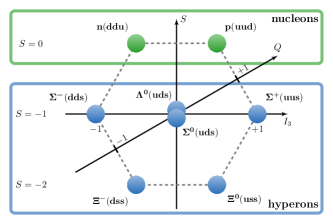
Figure 1: The spin-1/2 baryon octet where $S$, $I_{3}$ and $Q=(1+S)/2+I_{3}$ label strangeness, isospin and charge, respectively.

Baryon charges $g_{J}^{B^{\prime}B}$ are obtained from matrix elements of the form

$$\langle B^{\prime}(p^{\prime},s^{\prime})|\bar{u}\Gamma_{J}d|B(p,s)\rangle=g_{J}^{B^{\prime}B}\bar{u}_{B^{\prime}}(p^{\prime},s^{\prime})\Gamma_{J}u_{B}(p,s)$$ (1)

at zero four-momentum transfer $q^{2}=(p^{\prime}-p)^{2}=0$. Above, $u_{B}(p,s)$ denotes the Dirac spinor of a baryon $B$ with four momentum $p$ and spin $s$. We restrict ourselves to $\Delta I_{3}=1$ transitions within the baryon octet. In this case $p^{\prime}=p$, since in isosymmetric QCD $m_{B^{\prime}}=m_{B}$, and it is sufficient to set $\mathbf{p}=\bm{0}$. Rather than using the above $I_{3}=1$ currents $\bar{u}\Gamma_{J}d$ (where the vector and axial currents couple to the $W^{-}$ boson), it is convenient to define $I_{3}=0$ isovector currents,

$$\mathcal{O}_{J}(x)=\bar{u}(x)\Gamma_{J}u(x)-\bar{d}(x)\Gamma_{J}d(x),$$ (2)

and the corresponding charges $g_{J}^{B}$,

$$\langle B(p,s)|\mathcal{O}_{J}|B(p,s)\rangle=g_{J}^{B}\bar{u}_{B}(p,s)\Gamma_{J}u_{B}(p,s),$$ (3)

which, in the case of isospin symmetry, are trivially related to the $g_{J}^{B^{\prime}B}$:

$$g_{J}^{N} \coloneqq g_{J}^{p}=g_{J}^{pn},$$ (4)

$$g_{J}^{\Sigma} \coloneqq g_{J}^{\Sigma^{+}}=-\sqrt{2}\,g_{J}^{\Sigma^{+}\Sigma^{0}},$$ (5)

$$g_{J}^{\Xi} \coloneqq g_{J}^{\Xi^{0}}=-g_{J}^{\Xi^{0}\Xi^{-}}.$$ (6)

Note that we do not include the $\Lambda$ baryon here since in this case the isovector combination trivially gives zero. We consider vector ($V$), axialvector ($A$), scalar ($S$) and tensor ($T$) operators which are defined through the Dirac matrices $\Gamma_{J}=\gamma_{4},\,\gamma_{i}\gamma_{5},\,\mathds{1},\,\sigma_{ij}$ for $J\in\{V,A,S,T\}$, with $\sigma_{\mu\nu}=\frac{1}{2}[\gamma_{\mu},\gamma_{\nu}]$, where $i,j\in\{1,2,3\}$ and $i<j$.

The axial charges in the $m_{s}=m_{\ell}=0$ chiral limit are important parameters in SU(3) ChPT and enter the expansion of every baryonic quantity. These couplings can be decomposed into two LECs $F$ and $D$ which appear in the first order meson-baryon Lagrangian for three light quark flavours (see, e.g., Ref. [27]):

$$g_{A}^{N}=F+D,\quad g_{A}^{\Sigma}=2F,\quad g_{A}^{\Xi}=F-D.$$ (7)

Due to group theoretical constraints, see, e.g., Refs. [28, 29], such a decomposition also holds for $m_{s}=m_{\ell}>0$, for the axial as well as for the other charges. We define for $m=m_{s}=m_{\ell}$

$$g_{J}^{N}(m) =F_{J}(m)+D_{J}(m),$$ (8)

$$g_{J}^{\Sigma}(m) =2F_{J}(m),$$ (9)

$$g_{J}^{\Xi}(m) =F_{J}(m)-D_{J}(m),$$ (10)

where $F=F_{A}(0)$, $D=D_{A}(0)$. The vector Ward identity (conserved vector current, CVC relation) implies that $g_{V}^{N}=g_{V}^{\Xi}=F_{V}=1$ and $g_{V}^{\Sigma}=2F_{V}$, i.e., in this case the above relations also hold for $m_{s}\neq m_{\ell}$, with $F_{V}(m)=1$ and $D_{V}(m)=0$.

In this article we determine the charges at many different positions in the quark mass plane and investigate SU(3) flavour symmetry breaking, i.e., the extent of violation of Eqs. (8)–(10). Due to this, other than for $J\neq V$ where $D_{V}/F_{V}=0$, the functions $D_{J}(m)$ and $F_{J}(m)$ are not uniquely determined at the physical point, where $m_{s}\gg m_{\ell}$. At this quark mass point we will find the approximate ratios $D_{A}/F_{A}\approx(1.55\mbox{ -- }1.95)$, $D_{S}/F_{S}\approx-(0.2\mbox{ -- }0.5)$ and $D_{T}/F_{T}\approx 1.5$. The first ratio can be compared to the SU(6) quark model expectation $D_{A}(m)/F_{A}(m)=3/2$ (see, e.g., ref. [30]), which is consistent with the large-$N_{c}$ limit [31].

III Lattice set-up

In this section we present the details of our lattice set-up. First, we describe the gauge ensembles employed and the construction of the correlation functions. The computation of the three-point correlation functions via a stochastic approach is briefly discussed. Following this, we present the fitting analysis and treatment of excited state contributions employed to extract the ground state baryon matrix elements. The renormalization factors used to match to the continuum $\overline{\text{MS}}$ scheme and the improvement factors utilized to ensure leading $O(a^{2})$ discretization effects are then given. Finally, the strategy for interpolation/extrapolation to the physical point in the infinite volume and continuum limit is outlined.

III.1 Gauge ensembles

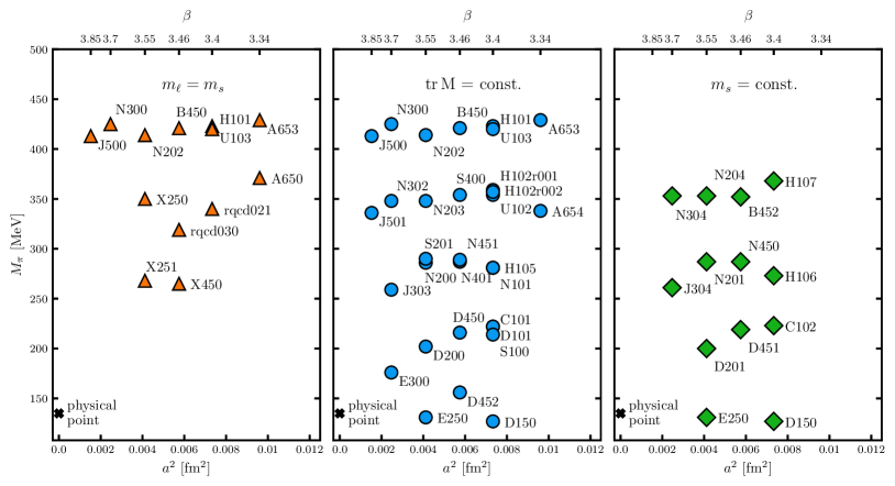
Figure 2: Parameter landscape of the ensembles listed in Table III.1. The ensembles are grouped according to the three quark mass trajectories (see the text and Fig. 3): (left) the symmetric line ($m_{\ell}=m_{s}$), (middle) the $\operatorname{tr}\,M=\text{const.}$ line and (right) the $m_{s}=\text{const.}$ line.

We employ ensembles generated with $N_{f}=2+1$ flavours of non-perturbatively $\mathcal{O}(a)$ improved Wilson fermions and a tree-level Symanzik improved gauge action, which were mostly produced within the Coordinated Lattice Simulations (CLS) [32] effort. Either periodic or open boundary conditions in time [33] are imposed, where the latter choice is necessary for ensembles with $a<0.06\,\text{fm}$ in order to avoid freezing of the topological charge and thus to ensure ergodicity [34]. The hybrid Monte Carlo (HMC) simulations are stabilized by introducing a twisted mass term for the light quarks [35], whereas the strange quark is included via the rational hybrid Monte Carlo (RHMC) algorithm [36]. The modifications of the target action are corrected for by applying the appropriate reweighting, see Refs. [32, 37, 17] for further details.

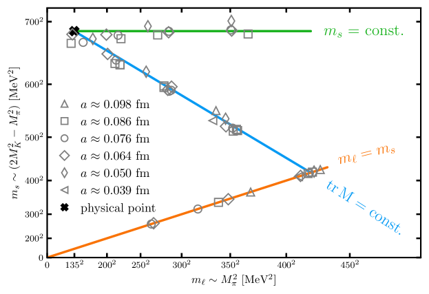
Figure 3: Position of the ensembles in the quark mass plane. The $\operatorname{tr}\,M=\text{const.}$ line (indicated as a blue line) and $m_{s}=\text{const.}$ line (green line) intersect close to the physical point (black cross). The symmetric line (orange line), which approaches the SU(3) chiral limit, crosses the $\operatorname{tr}\,M=\text{const.}$ line around $M_{\pi}=411\,\text{MeV}$.

In total 47 ensembles were analysed spanning six lattice spacings $a$ in the range $0.039\,\text{fm}\lesssim a\lesssim 0.098\,\text{fm}$, with pion masses between $430\,\text{MeV}$ and $130\,\text{MeV}$ (below the physical pion mass), as shown in Fig. 2. The lattice spatial extent $L$ is kept sufficiently large, where $LM_{\pi}\geq 4$ for the majority of the ensembles. A limited number of smaller volumes are employed to enable finite volume effects to be investigated, with the spatial extent varying across all the ensembles in the range $3.0\leq LM_{\pi}\leq 6.5$. Further details are given in Table III.1. The ensembles lie along three trajectories in the quark mass plane, as displayed in Fig. 3:

• the symmetric line: the light and strange quark masses are degenerate ($m_{\ell}=m_{s}$) and SU(3) flavour symmetry is exact.

• The $\operatorname{tr}\,M=\text{const.}$ line: starting at the $m_{\ell}=m_{s}$ flavour symmetric point, the trajectory approaches the physical point holding the trace of the quark mass matrix ($2m_{\ell}+m_{s}$, i.e., the flavour averaged quark mass) constant such that $2M_{K}^{2}+M_{\pi}^{2}$ is close to its physical value.

• The $m_{s}=\text{const.}$ line: the renormalized strange quark mass is kept near to its physical value [38].

The latter two trajectories intersect close to the physical point, whereas the symmetric line approaches the SU(3) chiral limit. In figures where data from different lines are shown, we will distinguish these, employing the symbol shapes of Fig. 2 (triangle, circle, diamond). The excellent coverage of the quark mass plane enables the interpolation/extrapolation of the results for the charges to the physical point to be tightly constrained. In addition, considering the wide range of lattice spacings and spatial volumes and the high statistics available for most ensembles, all sources of systematic uncertainty associated with simulating at unphysical quark mass, finite lattice spacing and finite volume can be investigated. Our strategy for performing a simultaneous continuum, quark mass and infinite volume extrapolation is given in Sec. III.6.

Table 1: List of the gauge ensembles analysed in this work. The rqcdxyz ensembles were generated by the RQCD group using the BQCD code [39], whereas all other ensembles were created within the CLS effort. Note that for H102 there are two replicas. These have the same parameters but were generated with slightly different algorithmic set-ups and, therefore, have to be analysed separately. N401 and N451 differ in terms of the boundary conditions (bc) imposed in the time direction (open (o) and anti-periodic (p), respectively). The lattice spacings $a$ are determined in Ref. [17]. In the second to last column $t$ denotes the source-sink separation of the connected three-point functions. The subscript (superscript) given for each separation indicates the number of measurements performed using the sequential source (stochastic) method on each configuration (see Secs. III.2 and III.3). The last column gives $N_{\text{cnfg}}$, the number of configurations analysed.

Ensemble	$\beta$	$a[\text{fm}]$	trajectory	bc	$N_{t}\cdot N_{s}^{3}$	$M_{\pi}[\text{MeV}]$	$M_{K}[\text{MeV}]$	$LM_{\pi}$	$t/a$	$N_{\text{cnfg}}$
A650	3.34	0.098	sym	p	$48\cdot 24^{3}$	371	371	4.43	$7_{3},9_{3},11_{3},13_{4}$	5062
A653			tr M/sym	p	$48\cdot 24^{3}$	429	429	5.12	$7_{3},9_{3},11_{3},13_{4}$	2525
A654			tr M	p	$48\cdot 24^{3}$	338	459	4.04	$7_{3}^{2},9_{3}^{2},11_{3}^{2},13_{4}^{2}$	2533
rqcd021	3.4	0.086	sym	p	$32\cdot 32^{3}$	340	340	4.73	$8_{2},10_{2},12_{4},14_{4}$	1541
H101			tr M/sym	o	$96\cdot 32^{3}$	423	423	5.88	$8_{2},10_{2},12_{2},14_{2}$	2000
U103			tr M/sym	o	$128\cdot 24^{3}$	420	420	4.38	$8_{1},10_{2},12_{3},14_{4}$	2470
H102r001			tr M	o	$96\cdot 32^{3}$	354	442	4.92	$8_{1}^{4},10_{2}^{4},12_{3}^{4},14_{4}^{4}$	997
H102r002			tr M	o	$96\cdot 32^{3}$	359	444	4.99	$8_{1}^{4},10_{2}^{4},12_{3}^{4},14_{4}^{4}$	1000
U102			tr M	o	$128\cdot 24^{3}$	357	445	3.72	$8_{1},10_{2},12_{3},14_{4}$	2210
N101			tr M	o	$128\cdot 48^{3}$	281	467	5.86	$8_{1},10_{2},12_{3},14_{4}$	1457
H105			tr M	o	$96\cdot 32^{3}$	281	468	3.91	$8_{1}^{2},10_{2}^{2},12_{3}^{2},14_{4}^{2}$	2038
D101			tr M	o	$128\cdot 64^{3}$	222	476	6.18	$8_{1},10_{2},12_{3},14_{4}$	608
C101			tr M	o	$96\cdot 48^{3}$	222	476	4.63	$8_{1}^{2},10_{2}^{2},12_{3}^{2},14_{4}^{2}$	2000
S100			tr M	o	$128\cdot 32^{3}$	214	476	2.98	$8_{1},10_{2},12_{3},14_{4}$	983
D150			tr M/ms	p	$128\cdot 64^{3}$	127	482	3.53	$8_{1},10_{2},12_{3},14_{4}$	603
H107			ms	o	$96\cdot 32^{3}$	368	550	5.12	$8_{2}^{2},10_{2}^{2},12_{3}^{2},14_{4}^{2}$	1564
H106			ms	o	$96\cdot 32^{3}$	273	520	3.80	$8_{2}^{4},10_{2}^{4},12_{3}^{4},14_{4}^{4}$	1553
C102			ms	o	$96\cdot 48^{3}$	223	504	4.65	$8_{2}^{4},10_{2}^{4},12_{3}^{4},14_{4}^{4}$	1500
rqcd030	3.46	0.076	sym	p	$64\cdot 32^{3}$	319	319	3.93	$9_{4},11_{4},13_{8},16_{8}$	1224
X450			sym	p	$64\cdot 48^{3}$	265	265	4.90	$9_{2},11_{2},13_{4},16_{4}$	400
B450			tr M/sym	p	$64\cdot 32^{3}$	421	421	5.19	$9_{3},11_{3},14_{3},16_{4}$	1612
S400			tr M	o	$128\cdot 32^{3}$	354	445	4.36	$9_{1}^{2},11_{2}^{2},13_{3},14^{2},16_{4}^{2}$	2872
N451			tr M	p	$128\cdot 48^{3}$	289	466	5.34	$9_{4}^{4},11_{4}^{4},13_{4},14^{4},16_{4}^{4}$	1011
N401			tr M	o	$128\cdot 48^{3}$	287	464	5.30	$9_{1}^{2},11_{2}^{2},13_{3},14^{2},16_{4}^{2}$	1086
D450			tr M	p	$128\cdot 64^{3}$	216	480	5.32	$9_{4}^{2},11_{4}^{2},13_{4},14^{2},16_{4}^{2}$	621
D452			tr M	p	$128\cdot 64^{3}$	156	488	3.84	$9^{4},11^{4},14^{4},16^{4}$	1000
B452			ms	p	$64\cdot 32^{3}$	352	548	4.34	$9_{3}^{2},11_{3}^{2},13_{3},14^{2},16_{4}^{2}$	1944
N450			ms	p	$128\cdot 48^{3}$	287	528	5.30	$9_{4}^{2},11_{4}^{2},13_{4},14^{2},16_{4}^{2}$	1132
D451			ms	p	$128\cdot 64^{3}$	219	507	5.39	$9_{4}^{2},11_{4}^{2},13_{4},14^{2},16_{4}^{2}$	458
X250	3.55	0.064	sym	p	$64\cdot 48^{3}$	350	350	5.47	$11_{2},14_{2},16_{4},19_{4}$	1493
X251			sym	p	$64\cdot 48^{3}$	268	268	4.19	$11_{4},14_{4},16_{8},19_{8}$	1474
N202			tr M/sym	o	$128\cdot 48^{3}$	414	414	6.47	$11_{1},14_{2},16_{2},19_{4}$	883
N203			tr M	o	$128\cdot 48^{3}$	348	445	5.44	$11_{1}^{4},14_{2}^{4},16_{3}^{4},19_{4}^{4}$	1543
N200			tr M	o	$128\cdot 48^{3}$	286	466	4.47	$11_{1}^{4},14_{2}^{4},16_{3}^{4},19_{4}^{4}$	1712
S201			tr M	o	$128\cdot 32^{3}$	290	471	3.02	$11_{1},14_{2},16_{3},19_{4}$	2092
D200			tr M	o	$128\cdot 64^{3}$	202	484	4.21	$11_{1}^{2},14_{2}^{2},16_{3}^{2},19_{4}^{2}$	2001
E250			tr M/ms	p	$192\cdot 96^{3}$	131	493	4.10	$11_{4},14_{4},16_{4},19_{4}$	490
N204			ms	o	$128\cdot 48^{3}$	353	549	5.52	$11_{2}^{2},14_{2}^{2},16_{3}^{2},19_{4}^{2}$	1500
N201			ms	o	$128\cdot 48^{3}$	287	527	4.49	$11_{2}^{2},14_{2}^{2},16_{3}^{2},19_{4}^{2}$	1522
D201			ms	o	$128\cdot 64^{3}$	200	504	4.17	$11_{1}^{4},14_{2}^{4},16_{3}^{4},19_{4}^{4}$	1078
N300	3.7	0.049	tr M/sym	o	$128\cdot 48^{3}$	425	425	5.15	$14_{1},17_{2},21_{2},24_{4}$	1539
N302			tr M	o	$128\cdot 48^{3}$	348	455	4.21	$14_{1}^{2},17_{2}^{2},21_{3}^{2},24_{4}^{2}$	1383
J303			tr M	o	$192\cdot 64^{3}$	259	479	4.18	$14_{2}^{2},17_{4}^{2},21_{6}^{2},24_{8}^{2}$	998
E300			tr M	o	$192\cdot 96^{3}$	176	496	4.26	$14_{3}^{2},17_{3}^{2},21_{6}^{2},24_{6}^{2}$	1038
N304			ms	o	$128\cdot 48^{3}$	353	558	4.27	$14_{2}^{2},17_{2}^{2},21_{3}^{2},24_{4}^{2}$	1652
J304			ms	o	$192\cdot 64^{3}$	261	527	4.21	$14_{3}^{2},17_{3}^{2},21_{3}^{2},24_{4}^{2}$	1630
J500	3.85	0.039	tr M/sym	o	$192\cdot 64^{3}$	413	413	5.24	$17_{1},22_{2},27_{3},32_{4}$	1837
J501			tr M	o	$192\cdot 64^{3}$	336	448	4.26	$17_{1}^{2},22_{2}^{2},27_{3}^{2},32_{4}^{2}$

III.2 Correlation functions

The baryon octet charges are extracted from two- and three-point correlation functions of the form

$$C_{\text{2pt}}^{B}(t)=\mathcal{P}_{+}^{\alpha\beta}\sum_{\mathbf{x}^{\prime}}\langle\mathcal{B}_{\alpha}(\mathbf{x}^{\prime},t)\;\bar{\mathcal{B}}_{\beta}(\mathbf{0},0)\rangle,$$ (11)

$$C_{\text{3pt}}^{B}(t,\tau)=\mathcal{P}^{\alpha\beta}\sum_{\mathbf{x}^{\prime},\mathbf{y}}\langle\mathcal{B}_{\alpha}(\mathbf{x}^{\prime},t)\mathcal{O}_{J}(\mathbf{y},\tau)\bar{\mathcal{B}}_{\beta}(\mathbf{0},0)\rangle.$$ (12)

Spin-1/2 baryon states are created (annihilated) using suitable interpolators $\overline{\mathcal{B}}$ ($\mathcal{B}$): for the nucleon, $\Sigma$ and $\Xi$, we employ interpolators corresponding to the proton, $\Sigma^{+}$ and $\Xi^{0}$, respectively,

$$N_{\alpha} =\epsilon^{ijk}u^{i}_{\alpha}\left(u^{jT}C\gamma_{5}d^{k}\right),$$ (13)

$$\Sigma_{\alpha} =\epsilon^{ijk}u^{i}_{\alpha}\left(s^{jT}C\gamma_{5}u^{k}\right),$$ (14)

$$\Xi_{\alpha} =\epsilon^{ijk}s^{i}_{\alpha}\left(s^{jT}C\gamma_{5}u^{k}\right),$$ (15)

with spin index $\alpha$, colour indices $i$, $j$, $k$ and $C$ being the charge conjugation matrix. The $\Lambda$ baryon is not considered here since three-point functions with the currents $\mathcal{O}_{J}=\bar{u}\Gamma_{J}u-\bar{d}\Gamma_{J}d$ vanish in this case. Without loss of generality, we place the source space-time position at the origin $(\mathbf{0},0)$ and the sink at $(\mathbf{x}^{\prime},t)$ such that the source-sink separation in time equals $t$. The current is inserted at $(\mathbf{y},\tau)$ with $0\leq\tau\leq t$. The annihilation interpolators are projected onto zero-momentum via the sums over the spatial sink position, while momentum conservation (and the sum over $\mathbf{y}$ for the current) means the source is also at rest.

Figure 4: Effective masses $m_{\text{eff}}^{B}(t)=\ln[C_{\text{2pt}}^{B}(t-\tfrac{a}{2})/C_{\text{2pt}}^{B}(t+\tfrac{a}{2})]/a$ of the nucleon (top) and $\Xi$ (bottom) determined on ensembles with $M_{\pi}\approx 340\,\text{MeV}$ and $M_{K}\approx 450\,\text{MeV}$ and lattice spacings ranging from $a=0.098\,\text{fm}$ (ensemble A654) down to $a=0.039\,\text{fm}$ (ensemble J501). The errors of $m^{B}_{\text{eff}}(t)$ are expected to increase in proportion to $a^{-1}$ but they also vary, e.g., with the number of effectively independent ensembles analysed.

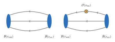
Figure 5: Quark-line diagrams of the two-point (left) and connected three-point (right) correlation functions where $x_{\text{src}}=(\mathbf{0},0)$, $x_{\text{ins}}=(\mathbf{y},\tau)$ and $x_{\text{snk}}=(\mathbf{x}^{\prime},t)$.

We ensure positive parity via the projection operator $\mathcal{P}_{+}=\frac{1}{2}(\mathds{1}+\gamma_{4})$. For the three-point functions, $\mathcal{P}=\mathcal{P}_{+}$ for $J=V,S$ and $\mathcal{P}=i\gamma_{i}\gamma_{5}\mathcal{P}_{+}$ for $J=A,T$. The latter corresponds to taking the difference of the polarizations (in the $i$ direction). The interpolators are constructed from spatially extended quark fields in order to increase the overlap with the ground state of interest and minimize contributions to the correlation functions from excited states. Wuppertal smearing is employed [20], together with APE-smeared [40] gauge transporters. The number of smearing iterations is varied with the aim of ensuring that ground state dominance sets in for moderate time separations. The root mean squared light quark smearing radii range from about $0.6\,\text{fm}$ (for $M_{\pi}\approx 430\,\text{MeV}$) up to about $0.8\,\text{fm}$ (for $M_{\pi}\approx 130\,\text{MeV}$), whereas the strange quark radii range from about $0.5\,\text{fm}$ (for the physical strange quark mass) up to about $0.7\,\text{fm}$ (for $M_{K}=M_{\pi}\approx 270\,\text{MeV}$). See Sec. E.1 (and in particular Table 15) of Ref. [17] for further details. Figure III.1 demonstrates that, when keeping for similar pion and kaon masses the smearing radii fixed in physical units, the ground state dominates the two-point functions at similar physical times across different lattice spacings.

Performing the Wick contractions for the two- and three-point correlation functions leads to the connected quark-line diagrams displayed in Fig. 5. Note that there are no disconnected quark-line diagrams for the three-point functions as these cancel when forming the isovector flavour combination of the current. The two-point functions are constructed in the standard way using point-to-all propagators. For the three-point functions either a stochastic approach (described in the next subsection) or the sequential source method [41] (on some ensembles in combination with the coherent sink technique [42]) is employed. The stochastic approach provides a computationally cost efficient way of evaluating the three-point functions for the whole of the baryon octet, however, additional noise is introduced. The relevant measurements for the nucleon (which has the worst signal-to-noise ratio of the octet) have already been performed with the sequential source method as part of other projects by our group, see, e.g., Ref. [43]. We use these data in our analysis and the stochastic approach for the correlation functions of the $\Sigma$ and the $\Xi$ baryons. Note that along the symmetric line ($m_{\ell}=m_{s}$) the hyperon three-point functions can be obtained as linear combinations of the contractions carried out for the currents $\bar{u}\Gamma_{J}u$ and $\bar{d}\Gamma_{J}d$ within the proton. Therefore, no stochastic three-point functions are generated in these cases.

We typically realize four source-sink separations with $t/\text{fm}\approx\{0.7,0.8,1.0,1.2\}$ in order to investigate excited state contamination and reliably extract the ground state baryon octet charges. Details of our fitting analysis are presented in Sec. III.4. Multiple measurements are performed per configuration, in particular for the larger source-sink separations to improve the signal, see Table III.1. The source positions are chosen randomly on each configuration in order to reduce autocorrelations. On ensembles with open boundary conditions in time only the spatial positions are varied and the source and sink time slices are restricted to the bulk of the lattice (sufficiently away from the boundaries), where translational symmetry is effectively restored.

III.3 Stochastic three-point correlation functions

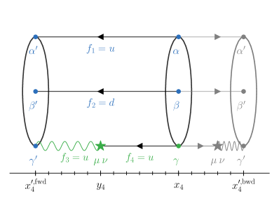
Figure 6: Schematic representation of the forward (left) and backward (right, shown in grey) propagating three-point correlation functions with open spin indices that are computed simultaneously with the stochastic approach. The indices corresponding to the spectator and insertion part from the factorization in Eq. (24) are colour-coded in blue and green, respectively. The black solid lines correspond to the standard point-to-all propagators, whereas the green wiggly lines represent stochastic timeslice-to-all propagators. The temporal positions of the forward/backward sink, insertion and source are labelled as $x_{4}^{\prime,\text{fwd}|\text{bwd}}$, $y_{4}$ and $x_{4}$, respectively. The flavour indices are chosen corresponding to a nucleon three-point function with a $\bar{u}\Gamma_{J}u$-current insertion.

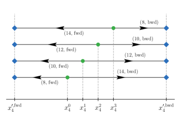
Figure 7: Sketch of the source and sink positions of the three-point functions realized using the stochastic approach. Blue diamonds depict the position of the forward ($x^{\prime,\text{fwd}}_{x}$) and backward ($x^{\prime,\text{bwd}}_{x}$) sink timeslices. Green points correspond to the source timeslices $x_{4}^{k}$ for $k=0,1,2,3$. Each three-point function measurement is labelled by the source-sink separation, where the values given correspond to the set-up for the ensembles at $\beta=3.40$.

In the following, we describe the construction of the connected three-point correlation functions using a computationally efficient stochastic approach. This method was introduced for computing meson three-point functions in Ref. [44] and utilized for baryons in Refs. [45, 46] and also for mesons in Refs. [47, 48]. Similar stochastic approaches have been implemented by other groups, see, e.g., Refs. [49, 50].

In Fig. 5 the quark-line diagram for the three-point function contains an all-to-all quark propagator which connects the current insertion at time $\tau$ with the baryon sink at time $t$. The all-to-all propagator is too computationally expensive to evaluate exactly. One commonly used approach avoids directly calculating the propagator by constructing a sequential source [41] which depends on the baryon sink interpolator (including its temporal position and momentum). This method has the disadvantage that one needs to compute a new quark propagator for each source-sink separation, sink momentum and baryon sink interpolator. Alternatively, one can estimate the all-to-all propagator stochastically. This introduces additional noise on top of the gauge noise, however, the quark-line diagram can be computed in a very efficient way. The stochastic approach allows one to factorize the three-point correlation function into a “spectator” and an “insertion” part which can be computed and stored independently with all spin indices and one colour index open. This is illustrated in Fig. 6 and explained in more detail below. The two parts can be contracted at a later (post-processing) stage with the appropriate spin and polarization matrices, such that arbitrary baryonic interpolators can be realized, making this method ideal for SU(3) flavour symmetry studies. Furthermore, no additional inversions are needed for different sink momenta.

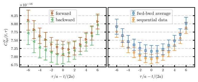
Figure 8: Left: polarized nucleon three-point correlation function propagating in the forward and backward directions for a $\bar{u}\gamma_{y}\gamma_{z}u$ current insertion obtained from one stochastic measurement on ensemble N200 ($a=0.064\,\text{fm}$). Note that two different source positions were needed to obtain the same source-sink separation $t=14a$ in the two directions, see Fig. 7. Right: forward-backward average of the stochastic three-point function shown on the left compared to that obtained using the sequential source method (with one source position, propagating in the forward direction).

As depicted in Fig. 7, we simultaneously compute the three-point functions for a baryon propagating (forwards) from source timeslice $x_{4}$ to sink timeslice $x_{4}^{\prime,\text{fwd}}$ and propagating (backwards) from $x_{4}$ to $x_{4}^{\prime,\text{bwd}}$. We start with the definition of the stochastic source and solution vectors which can be used to construct the timeslice-to-all propagator (shown as a green wiggly line in Fig. 6). In the following $i\in\{1,\dots,N_{\text{sto}}\}$ is the “stochastic index”, we denote spin indices with Greek letters, colour indices with Latin letters (other than $f$ or $i$) and we use flavour indices $f_{n}\in\{u,d,s\}$. We introduce (time partitioned) complex $\mathbb{Z}_{2}$ noise vectors [51, 52]

$$\eta_{i}(x)^{\alpha}_{a}=\left\{\begin{array}[]{ccl}\left(\mathbb{Z}_{2}\otimes\mathrm{i}\mathbb{Z}_{2}\right)/\sqrt{2}&\text{if}&x_{4}=x_{4}^{\prime,\text{fwd}|\text{bwd}}\\ \\ 0&&\text{otherwise}\ ,\end{array}\right.,$$ (19)

where the noise vector has support on timeslices $x_{4}^{\prime,\text{fwd}}$ and $x_{4}^{\prime,\text{bwd}}$. The noise vectors have the properties

$$\frac{1}{N_{\text{sto}}}\sum_{i=1}^{N_{\text{sto}}}\eta_{i}(x)^{\alpha}_{a} =\mathcal{O}\left(\frac{1}{\sqrt{N_{\text{sto}}}}\right),$$ (20)

$$\frac{1}{N_{\text{sto}}}\sum_{i=1}^{N_{\text{sto}}}\eta_{i}(x)^{\alpha}_{a}\eta^{*}_{i}(y)^{\beta}_{b} =\delta_{xy}\delta_{\alpha\beta}\delta_{ab}+\mathcal{O}\left(\frac{1}{\sqrt{N_{\text{sto}}}}\right).$$ (21)

The solution vectors $s_{f,i}(y)$ are defined through the linear system

$$D_{f}(x,y)^{\alpha\beta}_{ab}s_{f,i}(y)^{\beta}_{b}=\eta_{i}(x)^{\alpha}_{a},$$ (22)

where we sum over repeated indices (other than $f$) and $D_{f}(x,y)^{\alpha\beta}_{ab}$ is the Wilson-Dirac operator for the quark flavour $f$. Note that $s_{u,i}=s_{d,i}$ since our light quarks are mass-degenerate.

Using $\gamma_{5}$-Hermiticity ($\gamma_{5}D_{f}\gamma_{5}=D_{f}^{\dagger}$) and the properties given in Eqs. (20) and (21), the timeslice-to-all propagator connecting all points of the (forward and backward) sink timeslices $x_{4}^{\prime}$ to all points of any insertion timeslice $y_{4}$ can be estimated as

$$G_{f_{3}}(x^{\prime},y)^{\gamma^{\prime}\mu}_{c^{\prime}d}\approx\frac{1}{N_{\text{sto}}}\sum_{i=1}^{N_{\text{sto}}}\left[\gamma_{5}\eta_{i}(x^{\prime})\right]^{\gamma^{\prime}}_{c^{\prime}}\left[\gamma_{5}s^{*}_{f_{3}}(y)\right]^{\mu}_{d}.$$ (23)

Combining this timeslice-to-all propagator with point-to-all propagators for the source position $x_{4}$, the baryonic three-point correlation functions Eq. (12) can be factorized as visualized in Fig. 6 into a spectator part (S) and an insertion part (I), leaving all flavour and spin indices open:

$$C_{\text{3pt}} (\mathbf{p}^{\prime},\mathbf{q}|x_{4}^{\prime},y_{4},x_{4})^{\alpha^{\prime}\alpha\beta^{\prime}\beta\gamma^{\prime}\mu\nu\gamma}_{f_{1}f_{2}f_{3}f_{4}}$$

$$\approx\frac{1}{N_{\text{sto}}}\sum_{i=1}^{N_{\text{sto}}}\sum_{c=1}^{3}\Big{(}S_{f_{1}f_{2}}(\mathbf{p}^{\prime},x_{4}^{\prime},x_{4})^{\alpha^{\prime}\alpha\beta^{\prime}\beta\gamma^{\prime}}_{ic}$$

$$\qquad\qquad\qquad\qquad\qquad\times I_{f_{3}f_{4}}(\mathbf{q},y_{4},x_{4})^{\mu\nu\gamma}_{ic}\Big{)}.$$ (24)

The spectator and insertion parts are defined as

$$S_{f_{1}f_{2}} (\mathbf{p}^{\prime},x_{4}^{\prime},x_{4})^{\alpha^{\prime}\alpha\beta^{\prime}\beta\gamma^{\prime}}_{ic}$$

$$\coloneqq \sum_{\mathbf{x}^{\prime}}\Big{(}\epsilon_{a^{\prime}b^{\prime}c^{\prime}}\epsilon_{abc}G_{f_{1}}(x^{\prime},x)^{\alpha^{\prime}\alpha}_{a^{\prime}a}G_{f_{2}}(x^{\prime},x)^{\beta^{\prime}\beta}_{b^{\prime}b}$$

$$\qquad\qquad\qquad\qquad\times\big{[}\gamma_{5}\eta_{i}(x^{\prime})\big{]}^{\gamma^{\prime}}_{c^{\prime}}\;e^{-i\mathbf{p}^{\prime}\cdot(\mathbf{x}^{\prime}-\mathbf{x})}\Big{)},$$ (25)

$$I_{f_{3}f_{4}} (\mathbf{q},y_{4},x_{4})^{\mu\nu\gamma}_{ic}$$

$$\coloneqq\sum_{\textbf{y}}\left[\gamma_{5}s^{*}_{f_{3},i}(y)\right]^{\mu}_{d}G_{f_{4}}(y,x)^{\nu\gamma}_{dc}\;e^{+i\mathbf{q}\cdot(\mathbf{y}-\mathbf{x})}.$$ (26)

Using these building blocks, three-point functions for given baryon interpolators and currents for any momentum combination can be constructed. Note that in this article we restrict ourselves to the case $\mathbf{q}=\mathbf{p}^{\prime}={\bf 0}$. The point-to-all propagators within the spectator part are smeared at the source and at the sink, whereas $G_{f_{4}}$ is only smeared at the source. The stochastic source is smeared too, however, this is carried out after solving Eq. (22). In principle, the spectator part also depends on $f_{3}$ because for $f_{3}=s$ and $f_{3}\in\{u,d\}$ different smearing parameters are used. We ignore the dependence of the spectator part on $f_{3}$ since here we restrict ourselves to $f_{3},f_{4}\in\{u,d\}$. For details on the smearing see the previous subsection. Using the same set of timeslice-to-all propagators, we compute point-to-all propagators for a number of different source positions at timeslices $x_{4}$ in-between $x_{4}^{\prime,\text{bwd}}$ and $x_{4}^{\prime,\text{fwd}}$ which allows us to vary the source-sink distances, see Figs. 6 and 7.

The number of stochastic estimates $N_{\text{sto}}$ is chosen by balancing the computational cost against the size of the stochastic noise introduced. We find that for $N_{\text{sto}}\gtrsim 100$ the stochastic noise becomes relatively small compared to the gauge noise and we employ 100 estimates across all the ensembles. In some channels the signal obtained for the three-point function, after averaging over the forward and backward directions, is comparable to that obtained from the traditional sequential source method (for a single source, computed in the forward direction), as shown in Fig. 8. Nonetheless, when taking the ratio of the three-point function with the two-point function for the fitting analysis, discussed in the next subsection, a significant part of the gauge noise cancels, while the stochastic noise remains. This results in larger statistical errors in the ratio for the stochastic approach. This is a particular problem in the vector channel. A more detailed comparison of the two methods is given in Appendix A.

As mentioned above, only flavour conserving currents and zero momentum transfer are considered, however, the data to construct three-point functions with flavour changing currents containing up to one derivative for various different momenta is also available, enabling an extensive investigation of (generalized) form factors in the future. Similarly, meson three-point functions can be constructed by computing the relatively inexpensive meson spectator part and (re-)using the insertion part, see Ref. [48] for first results.

III.4 Fitting and excited state analysis

The spectral decompositions of the two- and three-point correlation functions read

$$C_{\text{2pt}}^{B}(t)=\sum_{n}|Z^{B}_{n}|^{2}e^{-E_{n}^{B}t}\ ,$$ (27)

$$C_{\text{3pt}}^{B}(t,\tau;\mathcal{O}_{J})=\sum_{n,m}Z^{B}_{n}Z^{B*}_{m}\langle n|\mathcal{O}_{J}|m\rangle e^{-E_{n}^{B}(t-\tau)}e^{E_{m}^{B}\tau},$$ (28)

where $E_{n}^{B}$ is the energy of state $|n\rangle$ ($n=0,1,\ldots$), created when applying the baryon interpolator $\bar{\mathcal{B}}$ to the vacuum state $|\Omega\rangle$ and $Z_{n}^{B}$ is the associated overlap factor $Z_{n}^{B}\propto\langle n|\bar{\mathcal{B}}|\Omega\rangle$. The ground state matrix elements of interest $\langle 0|\mathcal{O}_{J}|0\rangle=g_{J}^{B,\text{latt}}$ can be obtained in the limit of large time separations from the ratio of the three-point and two-point functions

$$R^{B}_{J}(t,\tau) =\frac{C^{B}_{\text{3pt}}(t,\tau;\mathcal{O}_{J})}{C^{B}_{\text{2pt}}(t)}\stackrel{{\scriptstyle t,\tau\rightarrow\infty}}{{\longrightarrow}}g_{J}^{B,\text{latt}}.$$ (29)

However, the signal-to-noise ratio of the correlation functions deteriorates exponentially with the time separation and with current techniques it is not possible to achieve a reasonable signal for separations that are large enough to ensure ground state dominance. At moderate $t$ and $\tau$, one observes significant excited state contributions to the ratio. All states with the same quantum numbers as the baryon interpolator contribute to the sums in Eqs. (27) and (28), including multi-particle excitations such as $B\pi$ P-wave and $B\pi\pi$ S-wave scattering states. The spectrum of states becomes increasingly dense as one decreases the pion mass while keeping the spatial extent of the lattice sufficiently large, where the lowest lying excitations are multi-particle states.

Table 2: Summary of the fits performed. We vary the combinations of channels $J$ that are fitted simultaneously as well as the number of excited states (ES) included in the fit and the fit interval $\tau\in[\delta t,t-\delta t]$ with $\delta t\in\{\delta t_{1},\delta t_{2}\}$, where $\delta t_{1}\approx 0.15\,\text{fm}$, $\delta t_{2}\approx 0.25\,\text{fm}$. The last two columns indicate which parameters in Eq. (30) are constrained by a prior or set to zero. All other parameters are determined in the fit.

Fit	$J$	$\delta t$	ES	prior	set to zero
1	$A,S,T$	$\delta t_{1}$	1	-	$b_{2}^{J}$, $b_{3}^{J}$, $b_{4}^{J}$, $\Delta E_{2}$
2	$A,S,T$	$\delta t_{2}$	1	-	$b_{2}^{J}$, $b_{3}^{J}$, $b_{4}^{J}$, $\Delta E_{2}$
3	$A,S,T,V$	$\delta t_{1}$	1	-	$b_{2}^{J}$, $b_{3}^{J}$, $b_{4}^{J}$, $\Delta E_{2}$
4	$A,S,T,V$	$\delta t_{2}$	1	-	$b_{2}^{J}$, $b_{3}^{J}$, $b_{4}^{J}$, $\Delta E_{2}$
5	$A,S,T$	$\delta t_{1}$	2	$\Delta E_{1}$	$b_{1}^{T}$, $b_{2}^{J}$, $b_{4}^{J}$
6	$A,S,T$	$\delta t_{2}$	2	$\Delta E_{1}$	$b_{1}^{T}$, $b_{2}^{J}$, $b_{4}^{J}$
7	$A,S,T,V$	$\delta t_{1}$	2	$\Delta E_{1}$	$b_{1}^{T,V}$, $b_{2}^{J}$, $b_{4}^{J}$
8	$A,S,T,V$	$\delta t_{2}$	2	$\Delta E_{1}$	$b_{1}^{T,V}$, $b_{2}^{J}$, $b_{4}^{J}$
9	$A,S,T$	$\delta t_{1}$	2	$\Delta E_{1}$	$b_{2}^{J}$, $b_{4}^{J}$
10	$A,S,T$	$\delta t_{2}$	2	$\Delta E_{1}$	$b_{2}^{J}$, $b_{4}^{J}$
11	$A,S,T,V$	$\delta t_{1}$	2	$\Delta E_{1}$	$b_{2}^{J}$, $b_{4}^{J}$
12	$A,S,T,V$	$\delta t_{2}$	2	$\Delta E_{1}$	$b_{2}^{J}$, $b_{4}^{J}$
13	$A,S,T$	$\delta t_{1}$	2	$\Delta E_{2}$	$b_{1}^{T}$, $b_{2}^{J}$, $b_{4}^{J}$
14	$A,S,T$	$\delta t_{2}$	2	$\Delta E_{2}$	$b_{1}^{T}$, $b_{2}^{J}$, $b_{4}^{J}$
15	$A,S,T,V$	$\delta t_{1}$	2	$\Delta E_{2}$	$b_{1}^{T,V}$, $b_{2}^{J}$, $b_{4}^{J}$
16	$A,S,T,V$	$\delta t_{2}$	2	$\Delta E_{2}$	$b_{1}^{T,V}$, $b_{2}^{J}$, $b_{4}^{J}$
17	$A,S,T$	$\delta t_{1}$	2	$\Delta E_{2}$	$b_{2}^{J}$, $b_{4}^{J}$
18	$A,S,T$	$\delta t_{2}$	2	$\Delta E_{2}$	$b_{2}^{J}$, $b_{4}^{J}$
19	$A,S,T,V$	$\delta t_{1}$	2	$\Delta E_{2}$	$b_{2}^{J}$, $b_{4}^{J}$
20	$A,S,T,V$	$\delta t_{2}$	2	$\Delta E_{2}$	$b_{2}^{J}$, $b_{4}^{J}$

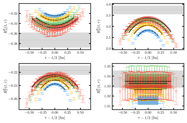
Figure 9: Unrenormalized ratios $R_{J}^{\Xi}(t,\tau)$, $J\in\{A,S,T,V\}$ (defined in Eq. (29)) for the cascade baryon on ensemble N302 ($M_{\pi}=348\,\text{MeV}$ and $a=0.049\,\text{fm}$), where $t\approx\{0.7,0.8,1.0,1.2\}\,\text{fm}$. The grey horizontal lines and bands show the results for the ground state matrix elements $\langle 0|\bar{u}\Gamma_{J}u-\bar{d}\Gamma_{J}d|0\rangle=g_{J}^{\Xi,\text{latt}}$, obtained from a simultaneous fit to the ratios for all channels and source-sink separations using parametrization 7 (see Eq. (30) and Table 2). The data points with $\tau\in\left[\delta t,t-\delta t\right]$, where $\delta t=2a$, are included in the fit (the faded data points are omitted), which is the maximum fit range possible for our action. The coloured curves show the expectation from the fit for each source-sink separation.

Figure 10: Results for the four unrenormalized charges of the nucleon (top) and cascade baryon (bottom) obtained from the fits listed in Table 2 for ensemble N302 ($M_{\pi}=348\,\text{MeV}$ and $a=0.049\,\text{fm}$). The green (blue) horizontal lines and bands indicate the final results and errors obtained from the median and 68% confidence level interval of the combined bootstrap distributions determined from the fits indicated by the green (blue) data points which include one (two) excited state(s). On the right the energy gaps determined in the fits and those corresponding to the lowest lying multi-particle states are displayed using the same colour coding as in Fig. 11.

One possible strategy is to first determine the energies of the ground state and lowest lying excitations by fitting to the two-point function (which is statistically more precise than the three-point function) with a suitable functional form. The energies can then be used in a fit to the three-point function (or the ratio $R_{J}^{B}$) to extract the charge $g_{J}^{B}$. However, the three-quark baryon interpolators we use by design have only a small overlap with the multi-particle states containing five or more quarks and antiquarks and it is difficult to extract the lower lying excited state spectrum from the two-point function. Nonetheless, multi-particle states can significantly contribute to the three-point function if the transition matrix elements $\langle n|{\cal O}_{J}|0\rangle$ are large. Furthermore, depending on the current, different matrix elements, and hence excited state contributions, will dominate. In particular, one would expect the axial and scalar currents to couple to the $B\pi$ P-wave and $B\pi\pi$ S-wave states, respectively, while the tensor and vector currents may enhance transitions between $B$ and $B\pi\pi$ states when $\pi\pi$ is in a P-wave.

The summation method [41] is an alternative approach, which involves summing the ratio over the operator insertion time $S_{J}^{B}(t)=\sum_{\tau=\tau_{0}}^{t-\tau_{0}}R^{B}_{J}(t,\tau)$, where one can show that the leading excited state contributions to $S_{J}^{B}(t)$ only depend on $t$ (rather than also on $t-\tau$ and $\tau$ as for $R^{B}_{J}(t,\tau)$). However, one needs a large number of source-sink separations (more than the four values of $t$ that are realized in this study) in order to extract reliable results from this approach.

These considerations motivate us to extract the charges by fitting to the ratio of correlation functions using a fit form which takes into account contributions from up to two excited states,

$$R^{B}_{J} (t,\tau)=b_{0}^{J}$$

$$+b_{1}^{J}\left(e^{-\Delta E_{1}(t-\tau)}+e^{-\Delta E_{1}\tau}\right)+b_{2}^{J}e^{-\Delta E_{1}t}$$

$$+b_{3}^{J}\left(e^{-\Delta E_{2}(t-\tau)}+e^{-\Delta E_{2}\tau}\right)+b_{4}^{J}e^{-\Delta E_{2}t}.$$ (30)

where $\Delta E_{n}=E_{n}^{B}-E_{0}^{B}$ denotes the energy gap between the ground state and the $n^{th}$ excited state of baryon $B$ and we have not included transitions between the first and the second excited state. The amplitude $b_{0}^{J}=g_{J}^{B,\text{latt}}$ gives the charge, while $b_{1,3}^{J}$ and $b_{2,4}^{J}$ are related to the ground state to excited state and excited state to excited state transition matrix elements, respectively. In practice, even when simultaneously fitting to all available source-sink separations, it is difficult to determine the energy gaps (and amplitudes) for a particular channel $J$. Similar to the strategy pursued in Ref. [53], we simultaneously fit to all four channels $J\in\{V,A,S,T\}$ for a given baryon. As the same energy gaps are present, the overall number of fit parameters is reduced and the fits are further constrained.

To ensure that the excited state contributions are sufficiently under control, we carry out a variety of different fits, summarized in Table 2. We vary

• the data sets included in the fit: simultaneous fits are performed to the data for $J\in\{A,S,T,V\}$ and $J\in\{A,S,T\}$. As the axial, scalar and tensor channels are the main focus of this study, we only consider excluding the vector channel data.

• the parametrization: either one (‘ES=1’) or two (‘ES=2’) excited states are included in the fits. In the latter case, in order to stabilize the fit, we use a prior for $\Delta E_{1}$ corresponding to the energy gap for the lowest lying multi-particle state. As a cross-check we repeat these fits using the average result obtained for $\Delta E_{2}$ in fits 5–8 as a prior and leaving $\Delta E_{1}$ as a free parameter (fits 13–20). The widths of the priors are set to $E_{1}/100$ and to $E_{2}/100$, respectively. In general, the contributions from excited state to excited state transitions could not be resolved and the parameters $b^{J}_{2,4}$ are set to zero. We also found that the tensor and vector currents couple more strongly to the second excited state, consistent with the expectations mentioned above, and the first excited state contributions are omitted for these channels in the ‘ES=2’ fits. Furthermore, due to the large statistical error of the stochastic three-point functions for the $\Sigma$ and $\Xi$ baryons in the vector channel (see Fig. 9 and the discussion in Appendix A), we are not able to resolve $b_{1}^{V}$ (and analogously $b_{3}^{V}$). For these baryons we also set $b_{1,3}^{V}=0$ in all the fits.

• the fit range: two fit intervals $\tau\in[\delta t_{j},t-\delta t_{j}]$ are used with $\delta t_{1}=n_{1}a\approx 0.15\,\text{fm}$ and $\delta t_{2}=n_{2}a\approx 0.25\,\text{fm}$.

A typical fit to the ratios for the cascade baryon is shown in Fig. 9 for ensemble N302 ($M_{\pi}=348\,\text{MeV}$ and $a=0.049\,\text{fm}$). The variation in the ground state matrix elements extracted from the 20 different fits is shown in Fig. III.1, also for the nucleon on the same ensemble. See Appendix C for the analogous plot for the $\Sigma$ baryon. Overall, the results are consistent within errors, however, some trends in the results can be seen across the different ensembles. In the axial channel, in particular the results for the fits involving a single excited state (fits 1–4), tend to be lower than those involving two excited states (fits 5–20). The former are, in general, statistically more precise than the latter due to the smaller number of parameters in the fit.

In order to study the systematics arising from any residual excited state contamination in the final results at the physical point (in the continuum limit at infinite volume), the extrapolations, detailed in Sec. III.6, are performed for the results obtained from fits 1–4 (‘ES=1’) and fits 5–8 (‘ES=2’), separately. For each set of fits, 500 samples are drawn from the combined bootstrap distributions of the four fit variations. The final result and error, shown as the green and blue bands in Fig. III.1, correspond to the median and the 68% confidence interval, respectively. Note that we take the same 500 bootstrap samples for all the baryons to preserve correlations. The final results for all the ensembles are listed in Tables B,  B and B of Appendix B for the nucleon, sigma and cascade baryons, respectively.

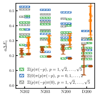
Figure 11: Results for the first and second excited state energy gaps of the cascade baryon, $\Delta E_{1}$ (brown data points) and $\Delta E_{2}$ (orange data points), respectively, determined on ensembles lying on the $\operatorname{tr}\,M=\text{const.}$ trajectory with $a=0.064\,\text{fm}$. The pion mass decreases from left to right with $M_{\pi}=414$ MeV for ensemble N202 and $M_{\pi}=202$ MeV for ensemble D200, see Table III.1. For each ensemble, the $\Delta E_{1}$ obtained using fits 1–4 of Table 2 are shown on the left and the $\Delta E_{1}$ (fixed with a prior to the lowest multi-particle energy gap) and $\Delta E_{2}$ resulting from fits 5–8 are displayed on the right. For comparison, the energy gaps of the lower lying non-interacting multi-particle states with the quantum numbers of the cascade baryon are shown as horizontal lines, where the momenta utilized for each hadron are indicated in lattice units.

In terms of the energy gaps extracted, Fig. III.1 shows that we find consistency across variations in the fit range and whether the vector channel data is included or not. However, the first excited energy gap $\Delta E_{1}$ obtained from the single excited state fits tends to be higher than the lowest multi-particle level, in particular, as the pion mass is decreased, suggesting that contributions from higher excited states are significant. This can be seen in Fig. 11, where we compare the results for the energy gaps for the cascade baryon with the lower lying non-interacting $\Xi\pi$ and $\Xi\pi\pi$ states for four ensembles with $a=0.064\,\text{fm}$ and pion masses ranging from $414\,\text{MeV}$ down to $202\,\text{MeV}$. Note that the multi-particle levels are modified in a finite volume, although the corresponding energy shifts may be small for the large volumes realized here. There are a number of levels within roughly $500\,\text{MeV}$ of the first excited state. Some levels lie close to each other and one would not expect that the difference can be resolved by fits with one or two excited states. The $\Delta E_{2}$ energy gaps from the two excited state fits (with the first excited state fixed with a prior to the lowest multi-particle level) are consistent with the next level that is significantly above the first excited state, although for ensemble D200 the errors are too large to draw a conclusion. Given that more than one excited state is contributing significantly, we expect that the latter fits isolate the ground state contribution more reliably. We remark that within present statistics, two-exponential fits to the two-point functions alone give energy gaps $a\Delta E=0.390(37),0.371(34),0.430(37)$ and $0.312(46)$ for N202, N203, N200 and D200, respectively, that are all larger than $a\Delta E_{2}$, with the exception of D200, where the two gaps agree within errors.

III.5 Non-perturbative renormalization and improvement

The isovector lattice charges, $g_{J}^{B,\text{latt}}$, extracted in the previous subsection need to be matched to the continuum $\overline{\text{MS}}$ scheme. The renormalized matrix elements suffer from discretization effects, however, the leading order effects are reduced to $O(a^{2})$ when implementing full $O(a)$ improvement. In the forward limit, in addition to using a non-perturbatively $O(a)$ improved fermion action, this involves taking mass dependent terms into account. The following multiplicative factors are applied,

$$g_{J}^{B}=Z^{k}_{J}\left(1+am_{\ell}b_{J}+3a\bar{m}\tilde{b}_{J}\right)g_{J}^{B,\text{latt}}+O(a^{2})\ ,$$ (31)

for $J\in\{V,A,S,T\}$, where $Z_{J}$ are the renormalization factors and $b_{J}$ and $\tilde{b}_{J}$ are the $O(a)$ improvement coefficients. Note that the renormalization factors for the scalar and tensor currents depend on the scale, $Z_{S,T}=Z_{S,T}(\mu)$, where we take $\mu=2\,\text{GeV}$. The vector Ward identity lattice quark mass $am_{q}$ is obtained from the hopping parameter $\kappa_{q}$ ($q=\ell,s$) and the critical hopping parameter $\kappa_{\text{crit}}$ via $am_{q}=\left(1/\kappa_{q}-1/\kappa_{\text{crit}}\right)/2$. $\bar{m}=(2m_{\ell}+m_{s})/3$ denotes the flavour averaged quark mass. The hopping parameters for all ensembles used within this work are tabulated in Table B of Appendix B. For $\kappa_{\text{crit}}$ we utilize the interpolation formula [17]

$$\frac{1}{\kappa_{\text{crit}}}=8-0.402454g^{2}\frac{1+0.28955g^{2}-0.1660g^{6}}{1+0.22770g^{2}-0.2540g^{4}}.$$ (32)

The improvement coefficients $b_{J}$ and $\tilde{b}_{J}$ are determined non-perturbatively in Ref. [54]. We make use of updated preliminary values, which will appear in a future publication [55]. These are listed in Tables 3 and 4, respectively. Note that no estimates of $\tilde{b}_{J}$ are available for $\beta=3.85$. Considering the size of the statistical errors, the general reduction of the $|\tilde{b}_{J}|$ values with increasing $\beta$ (and the decreasing $a$), at this lattice spacing we set $\tilde{b}_{J}=0$ for all $J$.

Table 3: Improvement coefficients $b_{J}$ for $J\in\{A,S,T,V\}$ from Refs. [54, 55].

$\beta$	$b_{A}$	$b_{S}$	$b_{T}$	$b_{V}$
3.34	1.249(16)	1.622(47)	1.471(11)	1.456(11)
3.4	1.244(16)	1.583(62)	1.4155(48)	1.428(11)
3.46	1.239(15)	1.567(74)	1.367(12)	1.410(13)
3.55	1.232(15)	1.606(98)	1.283(14)	1.388(17)
3.7	1.221(13)	1.49(11)	1.125(15)	1.309(22)
3.85	1.211(12)	1.33(16)	0.977(38)	1.247(26)

Table 4: Improvement coefficients $\tilde{b}_{J}$ for $J\in\{A,S,T,V\}$ from Refs. [54, 55]. Note that no results are available for $\beta=3.85$.

$\beta$	$\tilde{b}_{A}$	$\tilde{b}_{S}$	$\tilde{b}_{T}$	$\tilde{b}_{V}$
3.34	-0.06(28)	-0.24(55)	1.02(16)	1.05(13)
3.4	-0.11(13)	-0.36(23)	0.49(17)	0.41(11)
3.46	0.08(11)	-0.421(83)	0.115(19)	0.158(28)
3.55	-0.03(13)	-0.25(12)	0.000(37)	0.069(42)
3.7	-0.047(75)	-0.274(65)	-0.0382(60)	-0.031(18)

For the renormalization factors, we employ the values obtained in Ref. [56]. The factors are determined non-perturbatively in the RI^′-SMOM scheme [57, 58] and then (for $Z_{S}$ and $Z_{T}$) converted to the $\overline{\text{MS}}$ scheme using three-loop matching [59, 60, 61]. We remark that the techniques for implementing the Rome-Southampton method were extended in Ref. [56] to ensembles with open boundary conditions in time. This development enables us to utilize ensembles with $a<0.06\,\text{fm}$, where only open boundary conditions in time are available due to the need to maintain ergodicity.

Table 5: Set of renormalization factors taken from Ref. [56], denoted as $Z_{J}^{1}$ in the text. The factors are determined using the RI^′-SMOM scheme and the ‘fixed-scale method’ with the perturbative subtraction of lattice artefacts. For $Z_{A}$ and $Z_{V}$, the values correspond to those listed under $Z^{\prime}_{A}$ and $Z^{\prime}_{V}$, respectively, which are obtained using renormalization conditions consistent with the respective Ward identities. The statistical and systematic errors have been added in quadrature.

$\beta$	$Z_{A}$	$Z_{S}^{\overline{\text{MS}}}(2\,\text{GeV})$	$Z_{T}^{\overline{\text{MS}}}(2\,\text{GeV})$	$Z_{V}$
3.34	0.77610(58)	0.6072(26)	0.8443(35)	0.72690(71)
3.4	0.77940(36)	0.6027(25)	0.8560(35)	0.73290(67)
3.46	0.78240(32)	0.5985(25)	0.8665(36)	0.73870(71)
3.55	0.78740(22)	0.5930(25)	0.8820(37)	0.74740(82)
3.7	0.79560(98)	0.5846(24)	0.9055(42)	0.76150(94)
3.85	0.8040(13)	0.5764(25)	0.9276(42)	0.77430(76)

Table 6: Set of renormalization factors denoted as $Z_{J}^{2}$ in the text. These are determined as in Table 5 but now using the ‘fit method’.

$\beta$	$Z_{A}$	$Z_{S}^{\overline{\text{MS}}}(2\,\text{GeV})$	$Z_{T}^{\overline{\text{MS}}}(2\,\text{GeV})$	$Z_{V}$
3.34	0.7579(42)	0.6115(93)	0.8321(95)	0.7072(60)
3.4	0.7641(35)	0.6068(86)	0.8462(88)	0.7168(49)
3.46	0.7695(36)	0.6025(79)	0.8585(84)	0.7250(43)
3.55	0.7774(36)	0.5968(66)	0.8756(76)	0.7367(37)
3.7	0.7895(32)	0.5880(45)	0.9010(63)	0.7544(30)
3.85	0.8006(25)	0.5793(35)	0.9243(55)	0.7699(38)

Table 7: Renormalization factors $Z_{A}$ and $Z_{V}$ obtained from the interpolation formulas in Eqs. (C.7) and (C.8) in Ref. [62], denoted as $Z_{J}^{3}$ in the text.

$\beta$	$Z_{A}$	$Z_{V}$
3.34	0.7510(11)	0.7154(11)
3.4	0.75629(65)	0.72221(65)
3.46	0.76172(39)	0.72898(39)
3.55	0.76994(34)	0.73905(35)
3.7	0.78356(32)	0.75538(33)
3.85	0.79675(45)	0.77089(47)

A number of different methods are employed in Ref. [56] to determine the renormalization factors. In order to assess the systematic uncertainty arising from the matching in the final results for the charges at the physical point in the continuum limit, we make use of two sets of results, collected in Tables 5 and 6 and referred to as $Z_{J}^{1}$ and $Z_{J}^{2}$, respectively, in the following. The first set of results are extracted using the ‘fixed-scale method’, where the RI^′-SMOM factors are determined at a fixed scale (ignoring discretization effects), while the second set are obtained by fitting the factors as a function of the scale and the lattice spacing, the ‘fit method’. See Ref. [56] for further details. In both cases, lattice artefacts are reduced by subtracting the perturbative one-loop expectation. For the axial and vector currents, we also consider a third set of renormalization factors, $Z_{J}^{3}$, listed in Table 7, that are obtained with the chirally rotated Schrödinger functional approach [63], see Ref. [62]. We emphasize that employing the different sets of renormalization factors should lead to consistent results for the charges in the continuum limit.

III.6 Extrapolation strategy

In the final step of the analysis the renormalized charges $g_{J}^{B}$ determined at unphysical quark masses and finite lattice spacing and spatial volume are extrapolated to the physical point in the continuum and infinite volume limits. We employ a similar strategy to the one outlined in Ref. [64] and choose continuum fit functions of the form

$$g_{J}^{B}(M_{\pi},M_{K} ,L,a=0)=$$ (33)

$$c_{0}+c_{\pi}M_{\pi}^{2}+c_{K}M_{K}^{2}+c_{V}M_{\pi}^{2}\frac{e^{-LM_{\pi}}}{\sqrt{LM_{\pi}}}\ ,$$

to parameterize the quark mass and finite volume dependence, where $L$ is the spatial lattice extent and the coefficients $c_{X}$, $X\in\{0,\pi,K,V\}$ are understood to depend on the baryon $B$ and the current $J$. The leading order coefficients $c_{0}$ give the charges in the SU(3) chiral limit, which can be expressed in terms of two LECs, e.g., $F$ and $D$, for the axial charges, see Eq. (7).

Equation (33) is a phenomenological fit form based on the SU(3) ChPT expressions for the axial charge. It contains the expected $O(p^{2})$ terms for the quark mass dependence and the dominant finite volume corrections. The $O(p^{3})$ expressions for $g_{A}^{B}$ [65, 66, 67] contain log terms with coefficients completely determined by the LECs $F$ and $D$. In an earlier study of the axial charges on the $m_{s}=m_{\ell}$ subset of the ensembles used here [64], we found that including these terms did not provide a satisfactory description of the data. When terms arising from loop corrections that contain decuplet baryons are taken into account, additional LECs enter that are difficult to resolve. If the coefficient of the log term is left as a free parameter, one finds that the coefficient has the opposite sign to the ChPT expectation without decuplet loops. We made similar observations in this study and this is also consistent with the findings of previous works, see, e.g., Refs. [68, 69, 70]. Finite volume effects appear at $O(p^{3})$ with no additional LECs appearing in the coefficients. Again the signs of the corrections are the opposite to the trend seen in the data and, when included, it is difficult to resolve the effects of the decuplet baryons. As is shown in Sec. IV, the data for all the charges are well described when the fit form is restricted to the dominant terms, with free coefficients $c_{0}$, $c_{\pi}$, $c_{K}$ and $c_{V}$.

We remark that the same set of LECs appear in the $O(p^{2})$ SU(3) ChPT expressions for the three different octet baryons (for a particular charge). Ideally, one would carry out a simultaneous fit to the whole baryon octet (taking the correlations between the $g_{J}^{B}$ determined on the same ensemble into account). However, we obtain very similar results when fitting the $g_{J}^{B}$ individually compared to fitting the results for all the octet baryons simultaneously. For simplicity, we choose to do the former, such that the coefficients $c_{X}$ for the different baryons are independent of one another.

Lattice spacing effects also need to be taken into account and we add both mass independent and mass dependent terms to the continuum fit ansatz to give

$$g_{J}^{B}(M_{\pi},M_{K},L,a) =g_{J}^{B}(\mathcal{M}_{\pi},\mathcal{M}_{K},L,0)$$

$$+c_{a}\;\mathbbm{a}^{2}+\bar{c}_{a}\overline{\mathcal{M}}^{2}\;\mathbbm{a}^{2}+\delta c_{a}\delta\mathcal{M}^{2}\;\mathbbm{a}^{2}$$

$$+c_{a,3}\;\mathbbm{a}^{3},$$ (34)

where $\overline{\mathcal{M}}^{2}=(2\mathcal{M}_{K}^{2}+\mathcal{M}_{\pi}^{2})/3$ and $\delta\mathcal{M}^{2}=\mathcal{M}_{K}^{2}-\mathcal{M}_{\pi}^{2}$. The meson masses are rescaled with the Wilson flow scale $t_{0}$ [71], $\mathcal{M}_{\pi,K}=\sqrt{8t_{0}}M_{\pi,K}$ to form dimensionless combinations. This rescaling is required to implement full $O(a)$ improvement (along with employing a fermion action and isovector currents that are non-perturbatively $O(a)$ improved) when simulating at fixed bare lattice coupling instead of at fixed lattice spacing, see Sec. 4.1 of Ref. [17] for a detailed discussion of this issue. The values of $t_{0}/a^{2}$ and the pion and kaon masses in lattice units for our set of ensembles are given in Table B of Appendix B. We translate between different lattice spacings using $t_{0}^{\star}$, the value of $t_{0}$ along the symmetric line where $12t_{0}^{*}M_{\pi}^{2}=1.110$ [72], i.e., $\mathbbm{a}={a}/{\sqrt{8t_{0}^{\star}}}$. The values, determined in Ref. [17], are listed in Table 8. Note that we include a term that is cubic in the lattice spacing in the fit form, however, this term is only utilized in the analysis of the vector charge, for which we have the most precise data.

Table 8: Values for $t_{0}^{\star}/a^{2}$ at each $\beta$-value as determined in Ref. [17].

$\beta$	3.34	3.4	3.46	3.55	3.7	3.85
$\tfrac{t_{0}^{\star}}{a^{2}}$	2.204(6)	2.888(8)	3.686(11)	5.157(15)	8.617(22)	13.988(34)

To obtain results at the physical quark mass point, we make use of the scale setting parameter

$$\sqrt{8t_{0,\text{phys}}}=0.4098^{(20)}_{(25)}\,\text{fm},$$ (35)

determined in Ref. [17] and take the isospin corrected pion and kaon masses quoted in the FLAG 16 review [73] to define the physical point in the quark mass plane,

$$M_{\pi}^{\text{phys}} =134.8(3)\,\text{MeV},$$ (36)

$$M_{K}^{\text{phys}} =494.2(3)\,\text{MeV}.$$ (37)

In practice, we choose to fit to the bare lattice charges $g_{J}^{B,\text{latt}}$ rather than the renormalized ones as this enables us to include the uncertainties of the renormalization and improvement factors (which are the same for all ensembles at fixed $\beta$) consistently. Therefore, our final fit form reads

$$g_{J}^{B,\text{latt}}=\frac{g_{J}^{B}(M_{\pi},M_{K},L,a)}{Z^{k}_{J}(\beta)\left(1+am_{\ell}b_{J}(\beta)+3a\bar{m}\tilde{b}_{J}(\beta)\right)},$$ (38)

where the dependence of the factors on the $\beta$-value is made explicit and the superscript $k$ of $Z_{J}^{k}$ refers to the different determinations of the renormalization factors that we consider, $k=1,2,3$ for $J\in\{A,V\}$ and $k=1,2$ for $J\in\{S,T\}$ (see Tables 5, 6 and 7 in the previous subsection). We introduce a separate parameter for $Z^{k}_{J}$, $b_{J}$ and $\tilde{b}_{J}$ for each $\beta$-value and add corresponding “prior” terms to the $\chi^{2}$ function. The statistical uncertainties of these quantities are incorporated by generating pseudo-bootstrap distributions.

The systematic uncertainty in the determination of the charges at the physical point is investigated by varying the fit model and by employing different cuts on the ensembles that enter the fits. For the latter we consider

1. no cut: including all the available data points, denoted as data set 0, DS$(0)$,

2. pion mass cut: excluding all ensembles with $M_{\pi}>400\,\text{MeV}$, DS($M_{\pi}^{\footnotesize{<400\,\text{MeV}}}$),

3. pion mass cut: excluding all ensembles with $M_{\pi}>300\,\text{MeV}$, DS($M_{\pi}^{\footnotesize{<300\,\text{MeV}}}$),

4. a lattice spacing cut: excluding the coarsest lattice spacing, i.e., the ensembles with $a\approx 0.098\,\text{fm}$, DS($a^{\footnotesize{<0.1\,\text{fm}}}$),

5. a volume cut: excluding all ensembles with $LM_{\pi}<4$, DS($LM_{\pi}^{\footnotesize{>4}}$).

In some cases, more than one cut is applied, e.g., cut 2 and 4, with the data set denoted DS($M_{\pi}^{\footnotesize{<400\,\text{MeV}}}$, $a^{\footnotesize{<0.1\,\text{fm}}}$), etc.. Our final results are obtained by carrying out the averaging procedure described in Appendix B of Ref. [64] which gives an average and error that incorporates both the statistical and systematic uncertainties.

IV Extrapolations to the continuum, infinite volume, physical quark mass limit

We present the extrapolations to the physical point in the continuum and infinite volume limits of the isovector vector ($V$), axial ($A$), scalar ($S$) and tensor ($T$) charges for the nucleon ($N$), sigma ($\Sigma$) and cascade ($\Xi$) octet baryons.

IV.1 Vector charges

The isovector vector charges for the nucleon, cascade and sigma baryons are $g_{V}^{N}=g_{V}^{\Xi}=1$ and $g_{V}^{\Sigma}=2$, up to second order isospin breaking corrections [74]. These values also apply to our isospin symmetric lattice results in the continuum limit for any quark mass combination and volume. A determination of the vector charges provides an important cross-check of our analysis methods and allows us to demonstrate that all systematics are under control.

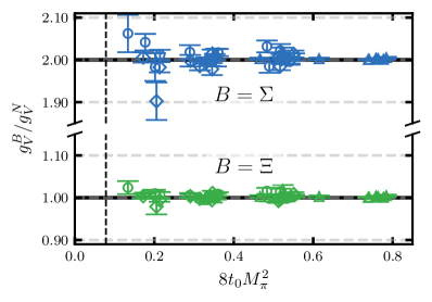
Figure 12: Ratio of the hyperon ($B=\Sigma,\Xi$) vector charges over the nucleon charge, $g_{V}^{B}/g_{V}^{N}$, as a function of the rescaled pion mass squared ($8t_{0}M_{\pi}^{2}=\mathcal{M}_{\pi}^{2}$). The data were extracted using two excited states in the fitting analysis, see Sec. III.4, and not corrected for lattice spacing or volume effects. Circles (diamonds) correspond to the $\operatorname{tr}M=\text{const.}$ ($m_{s}=\text{const.}$) trajectories, the triangles to the $m_{s}=m_{\ell}$ line.

To start with, we display the ratios of the hyperon charges over the nucleon charge in Fig. 12. The renormalization factors drop out in the ratio and lattice spacing effects are expected to cancel to some extent. As one can see, the results align very well with the expected values.

For the individual charges, we perform a continuum extrapolation of the data using the fit form

$$g_{V}= \;c_{0}+c_{a}\;\mathbbm{a}^{2}+\bar{c}_{a}\overline{\mathcal{M}}^{2}\;\mathbbm{a}^{2}+\delta c_{a}\delta\mathcal{M}^{2}\;\mathbbm{a}^{2}+c_{a,3}\;\mathbbm{a}^{3}.$$ (39)

Note that there is no dependence on the pion or kaon mass nor on the spatial volume in the continuum limit. $\mathcal{M}^{2}$ and $\delta\mathcal{M}^{2}$ represent the flavour average and difference of the kaon and pion masses squared, rescaled with the scale parameter $t_{0}$, while the lattice spacing $\mathbbm{a}=a/\sqrt{8t_{0}^{*}}$. See the previous section for further details of the extrapolation procedure. We implement full $O(a)$ improvement and leading discretization effects are quadratic in the lattice spacing. However, the data for the nucleon vector charge are statistically very precise and higher order effects can be resolved. This motivates the addition of the cubic term in Eq. (39). The data for $g_{V}^{\Sigma}$ and $g_{V}^{\Xi}$ are less precise as they are determined employing the stochastic approach outlined in Sec. III.3 which introduces additional noise, see Appendix A for further discussion.

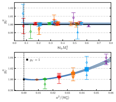
Figure 13: Continuum limit extrapolation of the nucleon isovector vector charge $g_{V}^{N}$ for a five parameter fit (Eq. (39)) using the renormalization factors $Z_{V}^{3}$ (see Table 7) and imposing the cut $M_{\pi}<400\,\text{MeV}$. The data were extracted including two excited states in the fitting analysis, see Sec. III.4. The upper panel shows the data points corrected for discretization effects according to the fit. They are consistent with $g_{V}^{N}=1$. The bottom panel shows the lattice spacing dependence at the physical point. The blue lines and grey bands indicate the expectations from the fit. For better visibility, the data point for ensemble D452, which has a relatively large error (see Table B), is not displayed. Circles (diamonds) correspond to the $\operatorname{tr}M=\text{const.}$ ($m_{s}=\text{const.}$) trajectories, the triangles to the $m_{s}=m_{\ell}$ line.

The data are well described by Eq. (39), as demonstrated by the fit, shown in Fig. 13, for $g_{V}^{N}$ which has a goodness of fit of $\chi^{2}/N_{\text{dof}}=0.92$. The data are extracted using two excited states in the fitting analysis (see Sec. III.4) and we employ the most precise determination of the renormalization factors ($Z_{V}^{3}$, see Table 7). A cut of $M_{\pi}<400$ MeV is imposed on the ensembles entering the fit, however, fits including all data points are also performed, as detailed below. When the data are corrected for the discretization effects according to the fit, we see consistency with $g_{V}^{N}=1$, for all pion and kaon masses. Using the fit to shift the data points to the physical point, we observe that the lattice spacing dependence is moderate but statistically significant, with a 3–4% deviation from the continuum value at the coarsest lattice spacing (lower panel of Fig. 13).

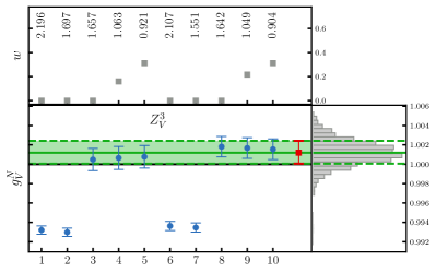
Figure 14: Results for the nucleon vector charge $g_{V}^{N}$ in the continuum limit at the physical point obtained using $Z_{V}^{3}$ (see Table 7) and five different parametrizations applied to data set DS($M_{\pi}^{\footnotesize{<400\,\text{MeV}}}$) (fits to Eq. (34) with different coefficients set to zero labelled 1,…,5, see the text) and DS($M_{\pi}^{\footnotesize{<400\,\text{MeV}}}$, $a^{\footnotesize{<0.1\,\text{fm}}}$) (6,…,10). See Sec. III.6 for the definitions of the data sets. The data were extracted including two excited states in the fitting analysis, see Sec. III.4. The model average is shown as the red data point and the green horizontal line and band. On the right the model averaged distribution is displayed as a histogram where also the median and the 68% confidence level interval, which form the final result, are indicated (green lines). The top panel shows the weights (grey points) assigned to the individual fits, with the corresponding $\chi^{2}/N_{\text{dof}}$ values given above.

In order to investigate the uncertainty arising from the choice of parametrization and the importance of the different terms, we repeat the extrapolations employing five different parametrizations (listed in terms of the coefficients of the terms entering the fit): $(1,\{c_{0},c_{a}\})$, $(2,\{c_{0},c_{a},\delta c_{a}\})$, $(3,\{c_{0},c_{a},c_{a,3}\})$, $(4,\{c_{0},c_{a},c_{a,3},\delta c_{a}\})$ and $(5,\{c_{0},c_{a},c_{a,3},\bar{c}_{a},\delta c_{a}\})$. Regarding the lattice spacing dependence, the mass independent term $c_{a}$ is always included as the other terms are formally at a higher order. These five fits are performed on two data sets. The first set contains ensembles with $M_{\pi}<400\,\text{MeV}$ (data set DS($M_{\pi}^{\footnotesize{<400\,\text{MeV}}}$)), while in the second set the ensembles with the coarsest lattice spacing are also excluded (DS($M_{\pi}^{\footnotesize{<400\,\text{MeV}}}$, $a^{\footnotesize{<0.1\,\text{fm}}}$), $+5$ is added to the fit number). See the end of Sec. III.6 for the definitions of the data sets.

The results for $g_{V}^{N}$, displayed in Fig. 14, show that the cubic term and at least one mass dependent term are needed to obtain a reasonable description of the data in terms of the $\chi^{2}/N_{\text{dof}}$. Two of the fit forms with large $\chi^{2}/N_{\text{dof}}$ values (corresponding to 1, 2, 6, 7, with negligible weight in the model averaging procedure) give values that are inconsistent with the continuum expectation. The results are stable under the removal of the coarsest ensembles. Performing the model averaging procedure, the final result for the nucleon, given in the last row of the first column of Table 9, agrees with the expectation $g_{V}^{N}=1$ within a combined statistical and systematic uncertainty of about 1‰.

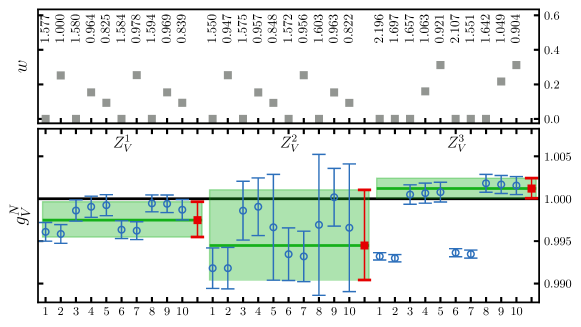
Figure 15: Results for the nucleon vector charge $g_{V}^{N}$ as in Fig. 14 but now also including those obtained employing $Z_{V}^{1}$ and $Z_{V}^{2}$.

The above analysis is also performed utilizing the sets of renormalization factors $Z_{V}^{1}$ and $Z_{V}^{2}$, determined via the RI^′-SMOM scheme [56]. The results for the nucleon vector charge are compared in Fig. 15. The uncertainties on these factors are larger, in particular for $Z_{V}^{2}$, than those of set $Z_{V}^{3}$, which is derived using the chirally rotated Schrödinger functional approach [62]. This translates into larger errors for $g_{V}^{N}$ for those fits. The lattice spacing dependence is somewhat different: the first quadratic mass dependent term in Eq. (39) and the cubic term can no longer be fully resolved and also parametrization $(2,\{c_{0},c_{a},\delta c_{a}\})$ gives a $\chi^{2}/N_{\text{dof}}=1.00$ (0.95) when employing $Z_{V}^{1}$ ($Z_{V}^{2}$).

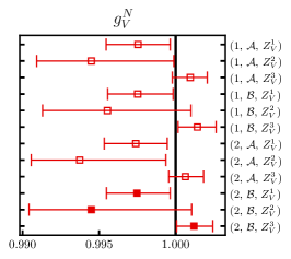
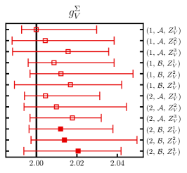
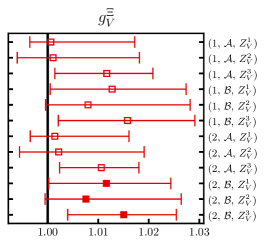
Figure 16: Overview of the results for the vector charges $g_{V}^{B}$, $B\in\{N,\Sigma,\Xi\}$, obtained from different data sets. These are labelled by the number of excited states used in the fitting analysis (ES=1, 2), the pion mass cut imposed (denoted $\mathcal{A}$ or $\mathcal{B}$) and the set of renormalization factors employed ($Z_{V}^{k}$, $k=1,2,3$). Each data point represents a model averaged result. The label $\mathcal{A}$ indicates that 15 fits (5 fit variations applied to three data sets, DS(0), DS($M_{\pi}^{\footnotesize{<400\,\text{MeV}}}$) and DS($a^{\footnotesize{<0.1\,\text{fm}}}$)) are averaged, while the results labelled with $\mathcal{B}$ are based on the set of 10 fits utilized in Fig. 14 (5 fit variations applied to two data sets, DS($M_{\pi}^{\footnotesize{<400\,\text{MeV}}}$) and DS($M_{\pi}^{\footnotesize{<400\,\text{MeV}}}$, $a^{\footnotesize{<0.1\,\text{fm}}}$)). See Sec. III.6 for the definitions of the data sets. The final results for each $Z_{V}^{k}$ (filled squares) are listed in Table 9.

The systematic uncertainty of the results due to residual excited state contamination and the range of pion masses employed in the extrapolations is also considered. Figure 16 shows the model averaged results discussed so far, displayed as filled squares, and also those obtained using several other sets of fits. These are labelled in terms of the number of excited states (one or two) included in the fitting analysis, the cuts imposed on the pion mass ($\mathcal{A}$ or $\mathcal{B}$) and the renormalization factors utilized. For the results from pion mass cut $\mathcal{A}$, 15 fits enter the model average, the five different parametrizations are applied to three data sets DS(0), DS($M_{\pi}^{\footnotesize{<400\,\text{MeV}}}$) and DS($a^{\footnotesize{<0.1\,\text{fm}}}$). Note that the first and third data set include ensembles with pion masses up to $430\,\text{MeV}$. For mass cut $\mathcal{B}$, data sets DS($M_{\pi}^{\footnotesize{<400\,\text{MeV}}}$) and DS($M_{\pi}^{\footnotesize{<400\,\text{MeV}}}$, $a^{\footnotesize{<0.1\,\text{fm}}}$)) are used, giving 10 fits in total. The results only depend on the choice of renormalization factors, suggesting that the systematic uncertainties due to excited state contamination and the cut made on the pion mass are very small.

Repeating the whole procedure for the sigma and the cascade baryons gives vector charges which are also consistent with the expected values to within $1.5\,\sigma$, as shown in Fig. 16 (see Figs. 41 and 42 in Appendix C for the individual fits for mass cut $\mathcal{B}$). The statistical noise introduced by the stochastic approach dominates, leading to much less precise values and very little variation between the results for the different hyperon data sets. We take the values obtained from the data sets (2, $\mathcal{B}$, $Z_{V}^{k}$), listed in Table 9, as our estimates of the vector charges as these data sets give the most reliable determinations of the charges across the different channels (as discussed in the following subsections).

Table 9: Results for $g_{V}^{B}$, $B\in\{N,\Sigma,\Xi\}$, obtained with three different sets of renormalization factors. The errors include the statistical and all the systematic uncertainties.

Renormalization	$g_{V}^{N}$	$g_{V}^{\Sigma}$	$g_{V}^{\Xi}$
$Z_{V}^{1}$ (Table 5)	$0.9975^{(22)}_{(20)}$	$2.012^{(26)}_{(16)}$	$1.012^{(13)}_{(11)}$
$Z_{V}^{2}$ (Table 6)	$0.9945^{(66)}_{(41)}$	$2.014^{(36)}_{(16)}$	$1.008^{(19)}_{(8)}$
$Z_{V}^{3}$ (Table 7)	$1.0012^{(12)}_{(11)}$	$2.021^{(21)}_{(27)}$	$1.015^{(10)}_{(11)}$

Overall, the results demonstrate that the systematics arising from excited state contamination, renormalization and finite lattice spacing are under control in our analysis in this channel (to within an error of 1‰ for the nucleon).

IV.2 Axial charges

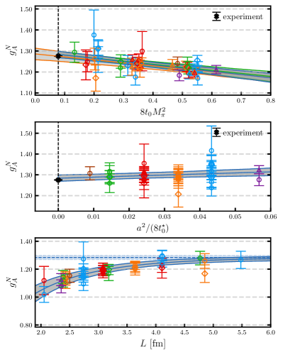
Figure 17: Simultaneous quark mass, continuum and finite volume extrapolation of the nucleon isovector axial charge $g_{A}^{N}$ extracted on ensembles with $M_{\pi}<400\,\text{MeV}$ using two excited states in the fitting analysis (see Sec. III.4) and renormalization factors $Z_{A}^{3}$ (see Table 7). A five parameter fit form is employed, see the text. (Top) Pion mass dependence of $g_{A}^{N}$, where the data points are corrected, using the fit, for finite volume and discretization effects and shifted (depending on the ensemble) to kaon masses corresponding to the $\operatorname{tr}\,M=\text{const.}$ and $m_{s}=\text{const.}$ trajectories. The fit is shown as a grey band with the three trajectories distinguished by blue ($\operatorname{tr}M=\text{const.}$, circles), green ($m_{s}=\text{const.}$, diamonds) and orange ($m_{s}=m_{\ell}$, triangles) lines, respectively. The vertical dashed line indicates the physical point. (Middle) Lattice spacing dependence at the physical point in the infinite volume limit. (Bottom) Finite volume dependence at the physical point in the continuum limit. The dashed blue line (band) indicates the infinite volume result. For better visibility, the data points for ensembles D150, E250 and D452, which have relatively large errors (see Table B), are not displayed. The black cross at the physical point indicates the experimental value [75].

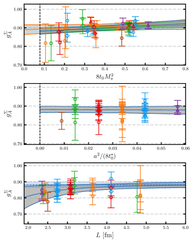
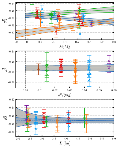
Figure 18: The same as Fig. 17 for the isovector axial charges $g_{A}^{B}$ of the sigma baryon (left) and the cascade baryon (right). For better visibility, the data points for ensembles D452 and D451, which have relatively large errors (see Table B), are not displayed for the cascade baryon. Compared to the nucleon, for the analysis of the hyperon charges a reduced set of ensembles is employed, see Tables B and B for a complete list of ensembles.

In the following we present our results for the nucleon, sigma and cascade isovector axial charges $g_{A}^{B}$, $B\in\{N,\Sigma,\Xi\}$. The nucleon axial charge is very precisely measured in experiment, $\lambda=g_{A}^{N}/g_{V}^{N}=1.2754(13)$ [75], and serves as another benchmark quantity when assessing the size of the systematics of the final results. Note, however, that possible differences of up to 2%, due to radiative corrections, between $\lambda$ computed in QCD and an effective $\lambda$ measured in experiment have been discussed recently [76, 77]. Lattice determinations of $g_{A}^{N}$ are known to be sensitive to excited state contributions, finite volume effects and other systematics. Whereas there is a long history of lattice QCD calculations of $g_{A}^{N}$, see, e.g., the FLAG 21 review [78], there are very few lattice computations of hyperon axial charges [22, 23, 24, 25, 26] and only few phenomenological estimates exist from measurements of semileptonic hyperon decay rates.

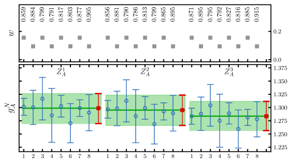
Figure 19: The same as Fig. 15 for the nucleon axial charge $g_{A}^{N}$. The eight fits correspond to two fit variations, see the text, applied to four data sets, DS($M_{\pi}^{\footnotesize{<400\,\text{MeV}}}$), DS($M_{\pi}^{\footnotesize{<300\,\text{MeV}}}$), DS($M_{\pi}^{\footnotesize{<400\,\text{MeV}}}$, $a^{\footnotesize{<0.1\,\text{fm}}}$) and DS($M_{\pi}^{\footnotesize{<400\,\text{MeV}}}$, $LM_{\pi}^{\footnotesize{>4}}$). The data are extracted using two excited states in the fitting analysis, see Sec. III.4.

We carry out simultaneous continuum, quark mass and finite volume fits to the individual baryon charges employing the parametrization in Eq. (34) (with the continuum form in Eq. (33)). The discretization effects are found to be fairly mild and we are not able to resolve the quadratic mass dependent terms or a cubic term. These terms are omitted throughout. As already mentioned in Sec. III.6 we are also not able to resolve any higher order ChPT terms in the continuum parametrization.

A five parameter fit, with free coefficients $\{c_{0},c_{\pi},c_{K},c_{V},c_{a}\}$, describes the data well, as demonstrated in Fig. 17 for the nucleon (with $\chi^{2}/N_{\text{dof}}=0.86$) and Fig. 18 for the sigma and cascade baryons (with $\chi^{2}/N_{\text{dof}}=0.85$ and 1.25, respectively). The data are extracted using two excited states (‘ES=2’) in the fitting analysis (see Sec. III.4) and renormalized with factors $Z_{A}^{3}$ (that are the most precise of the three determinations considered, see Table 7). For the cascade baryon, with two strange quarks, the data on the three quark mass trajectories ($\operatorname{tr}\,M=\text{const.}$, $m_{s}=\text{const.}$ and $m_{\ell}=m_{s}$) are clearly delineated, however, note the different scale on the right of Fig. 18. The availability of ensembles on two trajectories which intersect at the physical point helps to constrain the physical value of the axial charge. In terms of the finite volume effects, only the nucleon shows a significant dependence on the spatial extent. The quark mass dependence is also pronounced in this case.

As in the vector case, we quantify the systematics associated with the extraction of the charges at the physical point (in the continuum and infinite volume limits) by varying the parametrization and the set of ensembles that are included in the fit. We consider two fit forms $(1,\{c_{0},c_{\pi},c_{K},c_{V},c_{a}\})$ and $(2,\{c_{0},c_{\pi},c_{K},c_{V},c_{a},\delta c_{a}\}$) and four data sets, DS($M_{\pi}^{\footnotesize{<400\,\text{MeV}}}$), DS($M_{\pi}^{\footnotesize{<300\,\text{MeV}}}$), DS($M_{\pi}^{\footnotesize{<400\,\text{MeV}}}$, $a^{\footnotesize{<0.1\,\text{fm}}}$) and DS($M_{\pi}^{\footnotesize{<400\,\text{MeV}}}$, $LM_{\pi}^{\footnotesize{>4}}$), see Sec. III.6 for their definitions.

The results of the eight fits and their model averages for the three different determinations of the renormalization factors are shown in Fig. 19 for the nucleon and in Fig. 43 of Appendix C for the hyperon axial charges. In all cases, we find consistent results across the different fits and choice of renormalization factor suggesting that the statistical errors dominate. The additional lattice spacing term is not really resolved with the goodness of fit only changing slightly, while the errors on the coefficients increase. For the nucleon and sigma baryon, all fits have a $\chi^{2}/N_{\text{dof}}<1$ and are given a similar weight in the model average, while for the cascade baryon, the cut $M_{\pi}^{\footnotesize{<300\,\text{MeV}}}$ is needed to achieve a goodness of fit around 1 and these fits have the highest weight factors.

In order to further explore the systematics, additional data sets are considered. We assess the sensitivity of the results to excited state contributions by performing extrapolations of the data extracted using only one excited state (‘ES=1’) in the fitting analysis. In addition, as only the $O(p^{2})$ ChPT terms are included in the continuum parametrization, we test the description of the quark mass dependence by performing 10 fits, involving the two parametrization variations above, applied to five data sets, DS(0), DS($M_{\pi}^{\footnotesize{<400\,\text{MeV}}}$), DS($M_{\pi}^{\footnotesize{<300\,\text{MeV}}}$), DS($a^{\footnotesize{<0.1\,\text{fm}}}$) and DS($LM_{\pi}^{\footnotesize{>4}}$). The first, fourth and fifth data sets include ensembles with pion masses up to $430\,\text{MeV}$.

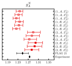
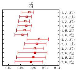
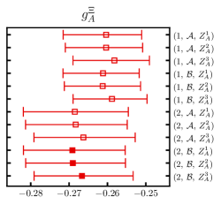
Figure 20: The same as Fig. 16 for the nucleon, sigma and cascade axial charges. The label $\mathcal{A}$ indicates that 10 fits enter the model average corresponding to two fit variations, see the text, applied to 5 data sets, DS(0), DS($M_{\pi}^{\footnotesize{<400\,\text{MeV}}}$), DS($M_{\pi}^{\footnotesize{<300\,\text{MeV}}}$), DS($a^{\footnotesize{<0.1\,\text{fm}}}$) and DS($LM_{\pi}^{\footnotesize{>4}}$). For the data points labelled with $\mathcal{B}$, the results of the 8 fits employed in Fig. 19 are averaged. For the nucleon, the FLAG 21 average for $N_{f}=2+1$ [79, 53] and the experimental value [75] are indicated (black diamonds)

Table 10: Results for $g_{A}^{B}$, $B\in\{N,\Sigma,\Xi\}$, obtained with three different sets of renormalization factors. The errors include the statistical and all the systematic uncertainties.

Renormalization	$g_{A}^{N}$	$g_{A}^{\Sigma}$	$g_{A}^{\Xi}$
$Z_{A}^{1}$ (Table 5)	$1.299^{(28)}_{(29)}$	$0.885^{(30)}_{(42)}$	$-0.269^{(14)}_{(13)}$
$Z_{A}^{2}$ (Table 6)	$1.295^{(28)}_{(29)}$	$0.882^{(30)}_{(42)}$	$-0.269^{(14)}_{(12)}$
$Z_{A}^{3}$ (Table 7)	$1.284^{(28)}_{(27)}$	$0.875^{(30)}_{(39)}$	$-0.267^{(13)}_{(12)}$

The results for the axial charges from model averaging the 10 fits (denoted $\mathcal{A}$) employing the 5 data sets and also from the 8 fits (denoted $\mathcal{B}$) using the 4 data sets given above, for the ‘ES=1’ and ‘ES=2’ data and the different renormalization factors are displayed in Fig. 20. Very little variation is seen in the results in terms of the range of pion masses included and, as before, the renormalization factors employed, suggesting the associated systematics are accounted for within the combined statistical and systematic error (which includes the uncertainty due to lattice spacing and finite volume effects). However, the results are sensitive to the number of excited states included in the fitting analysis. This is only a significant effect for the nucleon, for which the ‘ES=1’ results lie around $2.5\,\sigma$ below experiment. Similar underestimates of $g_{A}^{N}$ have been observed in many earlier lattice studies [78].

As detailed in Sec. III.4, more than one excited state is contributing significantly to the ratio of three-point over two-point correlation functions and including two excited states in the fitting analysis enables the ground state matrix element to be isolated more reliably. Considering the pion mass cuts, to be conservative we take the results of the model averages of the $\mathcal{B}$ data sets (where all the ensembles have $M_{\pi}<400\,\text{MeV}$) as only the dominant mass dependent terms are included in the continuum parametrization. Our estimates, corresponding to the (‘ES=2’, $\mathcal{B}$, $Z_{A}^{k}$) results in Fig. 20, are listed in Table 10.

IV.3 Scalar charges

As there is no isovector scalar current interaction at tree-level in the Standard Model, the scalar charges cannot be measured directly in experiment. However, the conserved vector current (CVC) relation can be used to estimate the charges from determinations of the up and down quark mass difference, $\delta_{m}=m_{u}-m_{d}$, and the QCD contribution to baryon mass isospin splittings, e.g., between the mass of the proton and the neutron, $\Delta m^{\text{QCD}}_{N}$, (for $g_{S}^{N}$ see Eq. (58) below). Reference [80] finds $g_{S}^{N}=1.02(11)$ employing lattice estimates for $\delta_{m}$ and an average of lattice and phenomenological values for $\Delta m^{\text{QCD}}_{N}$, which is consistent with the FLAG 21 [78] $N_{f}=2+1$ result of $g_{S}^{N}=1.13(14)$ [53]. Estimates can also be made of the isovector scalar charges of the other octet baryons, see the discussion in Sec. V.1. Conversely, direct determinations of the scalar charges can be used to predict $\delta_{m}$, as presented in Sec. V.3. So far, there has been only one previous study of the hyperon scalar charges [26].

For the extrapolation of the scalar charges and the extraction of the value at the physical point, we follow the same procedures as for the axial channel, presented in the previous subsection. The five parameter fit (with coefficients $\{c_{0},c_{\pi},c_{K},c_{V},c_{a}\}$) can again account for the observed quark mass, lattice spacing and volume dependence as illustrated in Fig. 21 for the nucleon (with $\chi^{2}/N_{\text{dof}}=0.56$) and Fig. 46 of Appendix C for the sigma and cascade baryons (with $\chi^{2}/N_{\text{dof}}=0.97$ and 1.14, respectively). The data are extracted using two excited states in the fitting analysis. For both hyperons, the quark mass and lattice spacing effects can be resolved, in contrast to the nucleon, while for all baryons the dependence on the spatial volume is marginal. When investigating the systematics in the estimates of the charges at the physical point, we perform model averages of the results of ($\mathcal{A}$): 8 fits from the two fit variations (as for the axial case) and the four data sets, DS(0), DS($M_{\pi}^{\footnotesize{<400\,\text{MeV}}}$), DS($a^{\footnotesize{<0.1\,\text{fm}}}$) and DS($LM_{\pi}^{\footnotesize{>4}}$), ($\mathcal{B}$): 6 fits from the two fit variations to the three data sets DS($M_{\pi}^{\footnotesize{<400\,\text{MeV}}}$), DS($M_{\pi}^{\footnotesize{<400\,\text{MeV}}}$, $a^{\footnotesize{<0.1\,\text{fm}}}$) and DS($M_{\pi}^{\footnotesize{<400\,\text{MeV}}}$, $LM_{\pi}^{\footnotesize{>4}}$). Note that a cut on the pion mass $M_{\pi}<300\,\text{MeV}$ is not considered. The scalar matrix elements are generally less precise than the axial ones and utilizing such a reduced data set leads to instabilities in the extrapolation and spurious values of the coefficients.

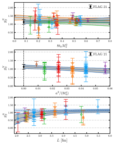
Figure 21: The same as Fig. 17 for the nucleon scalar charge $g_{S}^{N}$. The factors $Z_{S}^{1}$ are used for the matching (see Table 5). For orientation, the FLAG 21 result for $N_{f}=2+1$ [53] is indicated (black diamond) at the physical point. For better visibility, the data points for ensembles D150, E250 and D452, which have relatively large errors (see Table B), are not displayed.

Table 11: Results for $g_{S}^{B}$, $B\in\{N,\Sigma,\Xi\}$, obtained with two different sets of renormalization factors. The errors include the statistical and all the systematic uncertainties.

Renormalization	$g_{S}^{N}$	$g_{S}^{\Sigma}$	$g_{S}^{\Xi}$
$Z_{S}^{1}$ (Table 5)	$1.11^{(14)}_{(16)}$	$3.98^{(22)}_{(24)}$	$2.57^{(11)}_{(11)}$
$Z_{S}^{2}$ (Table 6)	$1.12^{(14)}_{(17)}$	$4.00^{(23)}_{(24)}$	$2.57^{(11)}_{(11)}$

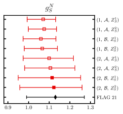
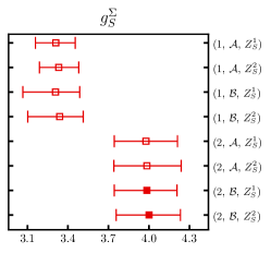
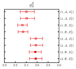
Figure 22: The same as Fig. 16 for the nucleon, sigma and cascade scalar charges. The label $\mathcal{A}$ indicates that 8 fits enter the model average corresponding to two fit variations, see the text, applied to 4 data sets, DS(0), DS($M_{\pi}^{\footnotesize{<400\,\text{MeV}}}$), DS($a^{\footnotesize{<0.1\,\text{fm}}}$) and DS($LM_{\pi}^{\footnotesize{>4}}$). For the data points labelled with $\mathcal{B}$, the two fit variations are performed on 3 data sets, DS($M_{\pi}^{\footnotesize{<400\,\text{MeV}}}$), DS($M_{\pi}^{\footnotesize{<400\,\text{MeV}}}$, $a^{\footnotesize{<0.1\,\text{fm}}}$) and DS($M_{\pi}^{\footnotesize{<400\,\text{MeV}}}$, $LM_{\pi}^{\footnotesize{>4}}$), giving a total of 6 fits for the average. For the nucleon, the FLAG 21 result for $N_{f}=2+1$ [53] is also shown (black diamond).

For illustration, the values from the individual fits and the model averages over the $\mathcal{B}$ data sets for the two different determinations of the renormalization factors are given in Fig. III.1 in Appendix C. The results are consistent across the different fits, although the weights vary. The values of the scalar charges for all the model averages performed are compiled in Fig. 22. There are no significant variations in the results obtained using the different renormalization factors and data sets ($\mathcal{A}$ or $\mathcal{B}$). For the nucleon, there is also agreement between the values for the data extracted including one (‘ES=1’) or two (‘ES=2’) excited states in the fitting analysis and consistency with the current FLAG 21 result. For the sigma baryon, and to a lesser extent for the cascade baryon, there is a tension between the ‘ES=1’ and ‘ES=2’ determinations. As discussed previously, the (‘ES=2’, $\mathcal{B}$, $Z_{S}^{k}$) values are considered the most reliable. These are listed in Table 11.

IV.4 Tensor charges

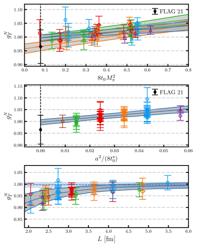
Figure 23: The same as Fig. 17 for the nucleon tensor charge $g_{T}^{N}$. The factors $Z_{T}^{1}$ are used for the matching (see Table 5). For orientation, the FLAG 21 result for $N_{f}=2+1$ [53] is indicated (black diamond) at the physical point. For better visibility, the data points for ensembles D150 and D452, which have relatively large errors (see Table B), are not displayed.

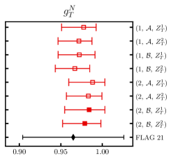
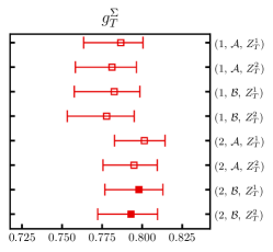
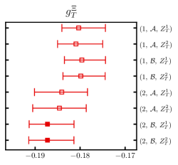
Figure 24: The same as Fig. 16 for the nucleon, sigma and cascade tensor charges. For the nucleon, the FLAG 21 result for $N_{f}=2+1$ [53] is also shown (black diamond).

In the isosymmetric limit, the nucleon tensor charge is equal to the first moment of the nucleon isovector transversity parton distribution function. Due to the lack of experimental data, estimates of $g_{T}^{N}$ from phenomenological fits have very large uncertainties, unless some assumptions are made. In fact, in some analyses, the fit is constrained to reproduce the lattice results for the isovector charge, see Refs. [14, 15]. The FLAG 21 review [78] gives as the $N_{f}=2+1$ value for the nucleon tensor charge the result of Ref. [53], $g_{T}^{N}=0.965(61)$, whereas, as far as we know, there is only one previous study of the hyperon tensor charges [26].

The extraction of the octet baryon tensor charges at the physical point follows the analysis of the axial charges in Sec. IV.2. In particular, the parametrizations employed and the data sets considered are the same. Figure 23 displays a typical example of an extrapolation for the nucleon tensor charge for a five parameter fit with a $\chi^{2}/N_{\text{dof}}=0.63$. See Fig. 47 in Appendix C for the analogous figures for the sigma and cascade baryons. The variation of the fits with the parametrization and the data sets utilized and the corresponding model averages, for the data sets with pion mass cut $\mathcal{B}$ (see Sec. IV.2), are shown in Fig. III.1.

Table 12: Results for $g_{T}^{B}$, $B\in\{N,\Sigma,\Xi\}$, obtained with two different sets of renormalization factors. The errors include the statistical and all the systematic uncertainties.

Renormalization	$g_{T}^{N}$	$g_{T}^{\Sigma}$	$g_{T}^{\Xi}$
$Z_{T}^{1}$ (Table 5)	$0.984^{(19)}_{(29)}$	$0.798^{(15)}_{(21)}$	$-0.1872^{(59)}_{(41)}$
$Z_{T}^{2}$ (Table 6)	$0.979^{(19)}_{(27)}$	$0.793^{(17)}_{(21)}$	$-0.1872^{(59)}_{(42)}$

An overview of the model averaged results for all variations of the input data is given in Fig. 24. The agreement between the different determinations suggests the systematics associated with the extrapolation are under control. Although the results utilizing data extracted with two excited states (‘ES=2’) in the fitting analysis are consistently above or below those extracted from the ‘ES=1’ data, considering the size of the errors of the model averages (which combine the statistical and systematic uncertainties), the differences are not significant. Our estimates for the tensor charges, corresponding to the (‘ES=2’, $\mathcal{B}$, $Z_{T}^{k}$) values, are listed in Table 12.

V Discussion of the results

Our values for the vector, axial, scalar and tensor charges of the nucleon, sigma and cascade baryons are given in Tables 9, 10, 11 and 12, respectively. In each case, we take the most precise value as our final result, i.e., the one obtained using $Z_{V}^{3}$ and $Z_{A}^{3}$ for the vector and axial channels, respectively, and $Z_{S}^{1}$ and $Z_{T}^{1}$ for the scalar and the tensor. In the following we compare with previous determinations of the charges taken from the literature and discuss the SU(3) flavour symmetry breaking effects in the different channels. We use the conserved vector current relation and our result for the scalar charge of the sigma baryon to determine the up and down quark mass difference. We compute the QCD contributions to baryon isospin mass splittings and evaluate the isospin breaking effects on the pion baryon $\sigma$ terms.

V.1 Individual charges

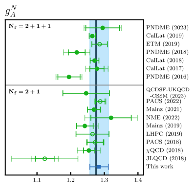
Figure 25: Compilation of recent lattice determinations of the nucleon axial charge $g_{A}^{N}$ with $N_{f}=2+1$ [81, 79, 82, 83, 53, 84, 85, 86, 26] and $N_{f}=2+1+1$ [87, 88, 68, 69, 89, 90, 91] dynamical fermions. Values with filled symbols were obtained via a chiral, continuum and finite volume extrapolation. The vertical black line gives the experimental result [75].

We first consider the axial charges. Our final values read

$$g_{A}^{N}=1.284^{(28)}_{(27)},\quad g_{A}^{\Sigma}=0.875^{(30)}_{(39)},\quad g_{A}^{\Xi}=-0.267^{(13)}_{(12)}.$$ (40)

The result for the nucleon compares favourably with the experimental value $g_{A}^{N}/g_{V}^{N}=1.2754(13)$ [75] and the FLAG 21 [78] average for $N_{f}=2+1$, $g_{A}^{N}=1.248(23)$. The latter is based on the determinations in Refs. [79, 53]. All sources of systematic uncertainty must be reasonably under control to be included in the FLAG average and a number of more recent studies incorporate continuum, quark mass and finite volume extrapolations. A compilation of results for $g_{A}^{N}$ is displayed in Fig. 25. Although the determinations are separated in terms of the number of dynamical fermions employed, including charm quarks in the sea is not expected to lead to a discernible effect.

Regarding the hyperon axial charges, far fewer works exist. Lin et al. [92, 22] performed the first study, utilizing $N_{f}=2+1$ ensembles with pion masses ranging between $350\,\text{MeV}$ and $750\,\text{MeV}$ and a single lattice spacing of $0.12\,\text{fm}$. After an extrapolation to the physical pion mass they obtain $g_{A}^{\Sigma}=0.900(42)_{\text{stat}}(54)_{\text{sys}}$ and $g_{A}^{\Xi}=-0.277(15)_{\text{stat}}(19)_{\text{sys}}$, where estimates of finite volume and discretization effects are included in the systematic uncertainty. Note that we have multiplied their result for $g_{A}^{\Sigma}$ by a factor of two to match our normalization convention. In Refs. [93, 24] ETMC determined all octet and decuplet (i.e., nucleon, hyperon and $\Delta$) axial couplings employing $N_{f}=2+1+1$ ensembles with pion masses between $210\,\text{MeV}$ and $430\,\text{MeV}$ and two lattice spacings $a\in\{0.065\,\text{fm},0.082\,\text{fm}\}$. Using a simple linear ansatz for the quark mass extrapolation, they quote $g_{A}^{\Sigma}=0.7629(218)_{\text{stat}}$ and $g_{A}^{\Xi}=-0.2479(87)_{\text{stat}}$, where the errors are purely statistical.

More recently, Savanur et al. [25] extracted the axial charges on $N_{f}=2+1+1$ ensembles with three different lattice spacings $a\in\{0.06\,\text{fm},0.09\,\text{fm},0.12\,\text{fm}\}$, pion masses between $135\,\text{MeV}$ and $310\,\text{MeV}$ and volumes in the range $3.3\leq LM_{\pi}\leq 5.5$. The ratios $g_{A}^{\Sigma}/g_{A}^{N}$ and $g_{A}^{\Xi}/g_{A}^{N}$ are extrapolated taking the quark mass dependence and lattice spacing and finite volume effects into account. The experimental value of $g^{N}_{A}$ is then used to obtain $g_{A}^{\Sigma}=0.891(11)_{\text{stat}}(13)_{\text{sys}}$ (again multiplied by a factor of two to meet our conventions) and $g_{A}^{\Xi}=-0.2703(47)_{\text{stat}}(13)_{\text{sys}}$. Finally, QCDSF-UKQCD-CSSM presented results for the isovector axial, scalar and tensor charges in Ref. [26]. They employ $N_{f}=2+1$ ensembles lying on a $\operatorname{tr}M=\text{const.}$ trajectory with pion masses ranging between $220\,\text{MeV}$ and $470\,\text{MeV}$ and five different values of the lattice spacing in the range $(0.052-0.082)\,\text{fm}$. The Feynman-Hellmann theorem is used to calculate the baryon matrix elements. Performing an extrapolation to the physical mass point including lattice spacing and finite volume effects, they find $g_{A}^{\Sigma}=0.876(26)_{\text{stat}}(09)_{\text{sys}}$ and $g_{A}^{\Xi}=-0.206(22)_{\text{stat}}(19)_{\text{sys}}$.

We also mention the earlier studies of Erkol et al. [23] ($N_{f}=2$), utilizing pion masses above $500\,\text{MeV}$, and QCDSF-UKQCD ($N_{f}=2+1$) carried out at a single lattice spacing [94].

Figure 26: Comparison of lattice determinations [22, 24, 25] of the hyperon axial charges for the $\Sigma$ and $\Xi$ baryons normalized to the nucleon axial charge. Some of the results from Lin et al. at heavier pion masses are not shown. The grey vertical dashed line indicates the physical pion mass point. Only our results from the $m_{s}=\text{const.}$ trajectory are shown. The grey bands indicate the (continuum limit, infinite volume) quark mass behaviour according to the fits displayed in Figs. 17 and 18. Note that the data points are not corrected for finite volume or discretization effects. All data are converted to our phase and normalization conventions, Eqs. (1)–(6). The Lin et al. and ETMC results are obtained by taking the ratio of the individual charges and employing error propagation.

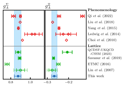
Figure 27: Comparison of our results for the axial charges $g_{A}^{\Sigma}$ and $g_{A}^{\Xi}$ (blue symbols and error bands) with other lattice determinations [22, 24, 25, 26] and phenomenological estimates [95, 67, 96, 97, 98]. Values with filled symbols were obtained via a chiral, continuum and finite volume extrapolation. All results are converted to our phase and normalization conventions, Eqs. (1)–(6).

In Fig. 26 we compare the ratios of the hyperon axial charges to the nucleon axial charge, $g_{A}^{B}/g_{A}^{N}$, from Refs. [22, 24, 25], obtained on individual ensembles to our results. A comparison of the charges themselves cannot be made since, as mentioned above, Savanur et al. only present results for the ratio. As the strange quark mass is held approximately constant in these works, only our results from the $m_{s}=\text{const.}$ trajectory are displayed. Similarly, the QCDSF-UKQCD-CSSM values are omitted as the ensembles utilized lie on a $\operatorname{tr}M=\text{const.}$ trajectory. We observe reasonable agreement between the data. Note that our continuum, infinite volume limit result (the grey band in the figure) for $g_{A}^{\Sigma}/g_{A}^{N}$ lies slightly below the central values of most of our $m_{s}=\text{const.}$ data points.

The individual hyperon axial charges at the physical point are shown in Fig. 27, along with a number of phenomenological determinations employing a variety of quark models [95, 97, 98], the chiral soliton model [96] and SU(3) covariant baryon ChPT [67]. Within errors, the lattice results are consistent apart from the rather low value for $g_{A}^{\Sigma}$ from ETMC [24] and the rather high value for $g_{A}^{\Xi}$ from QCDSF-UKQCD-CSSM [26]. The phenomenological estimates for $g_{A}^{\Sigma}$ are in reasonable agreement with our value, while there is a large spread in the expectations for $g_{A}^{\Xi}$.

We remark that, in analogy to the CVC relation (discussed in Sec. V.3 below), the axial Ward identity, $\partial_{\mu}(\bar{u}\gamma_{\mu}\gamma_{5}d)=i(m_{d}+m_{u})\bar{u}\gamma_{5}d$, connects the axial and pseudoscalar charges,

$$g^{B}_{P}=\frac{m_{B}}{m_{\ell}}g_{A}^{B},$$ (41)

where $m_{B}$ and $m_{\ell}$ correspond to the baryon and the light quark mass, respectively. This relation was employed in Ref. [80] to determine the pseudoscalar charge of the nucleon, which is defined as the pseudoscalar form factor in the forward limit. Taking the baryon masses of isosymmetric QCD from Table 14 of Ref. [17] and the isospin averaged light quark mass $m_{\ell}=3.381(40)\,\text{MeV}$ in the $N_{f}=4$ flavour $\overline{\text{MS}}$ scheme at $\mu=2\,\text{GeV}$ from the FLAG 21 review [78], we find

$$g_{P,N_{f}=4}^{N} =356^{(9)}_{(9)},\quad g_{P,N_{f}=4}^{\Sigma}=308^{(11)}_{(14)},$$

$$g_{P,N_{f}=4}^{\Xi} =-104^{(5)}_{(5)}.$$ (42)

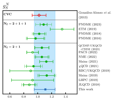
Figure 28: As in Fig. 25 for the nucleon scalar charge $g_{S}^{N}$ with $N_{f}=2+1$ [81, 83, 53, 99, 100, 85, 84, 86, 26] and $N_{f}=2+1+1$ [87, 69, 89, 91] dynamical fermions. González-Alonso et al. estimate the scalar charge via the conserved vector current (CVC) relation [80].

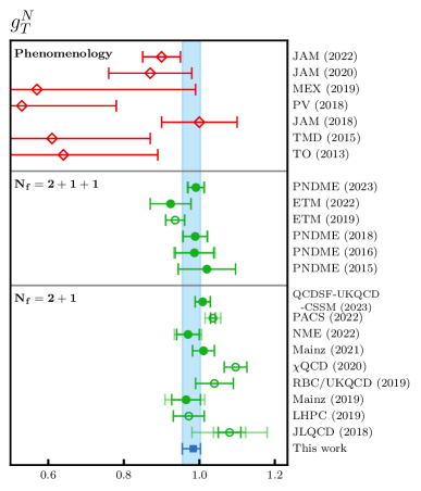
Figure 29: As in Fig. 25 for the nucleon tensor charge $g_{T}^{N}$ with $N_{f}=2+1$ [81, 83, 53, 99, 101, 85, 84, 86, 26] and $N_{f}=2+1+1$ [102, 87, 69, 89, 103, 91] dynamical fermions. Recent phenomenological estimates are also displayed for comparison [104, 105, 14, 106, 107, 108, 15]. Values with filled symbols were obtained via a quark mass, continuum and finite volume extrapolation. In addition, the filled ETM (2022) [103] point is obtained from a continuum limit extrapolation of results determined on three physical point ensembles with large spatial volumes.

Turning to the scalar charges, our final results in the three flavour $\overline{\text{MS}}$ scheme at $\mu=2\,\text{GeV}$ read

$$g_{S}^{N}=1.11^{(14)}_{(16)},\quad g_{S}^{\Sigma}=3.98^{(22)}_{(24)},\quad g_{S}^{\Xi}=2.57^{(11)}_{(11)}.$$ (43)

For the nucleon, our result for $g_{S}^{N}$ agrees with the FLAG 21 value $g_{S}^{N}=1.13(14)$ for $N_{f}=2+1$ [78] (taken from Ref. [53]) and more recent lattice determinations, see Fig. 28. There is only one previous lattice determination of the hyperon scalar couplings by QCDSF-UKQCD-CSSM [26], who obtain $g_{S}^{\Sigma}=2.80(24)_{\text{stat}}(05)_{\text{sys}}$ and $g_{S}^{\Xi}=1.59(11)_{\text{stat}}(04)_{\text{sys}}$. These values are much smaller than ours.

One can also employ the CVC relation and estimates of the QCD contribution to the isospin mass splittings and the light quark mass difference to determine the scalar charges. For a detailed discussion see Sec. V.3 below. Ref. [80] obtains $g_{S}^{N}=1.02(11)$ assuming $\Delta m_{N}^{\text{QCD}}=m^{\text{QCD}}_{p}-m^{\text{QCD}}_{n}=-2.58(18)\,\text{MeV}$ and the quark mass difference $\delta_{m}=m_{u}-m_{d}=-2.52(19)\,\text{MeV}$. Similarly, using the results by BMWc on the light quark mass splitting [116] and their QCD contributions to the baryon mass splittings [117], we obtain

$$g_{S}^{N}=1.05(13),\quad g_{S}^{\Sigma}=3.35(19),\quad g_{S}^{\Xi}=2.29(15),$$ (44)

which agree with our results to within two standard deviations. Note that a smaller value for $|\delta_{m}|$ (see Sec. V.3) would uniformly increase these charges.

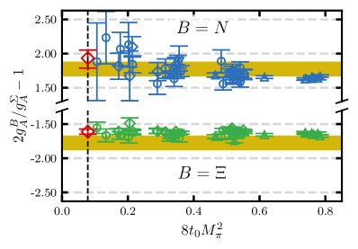
Figure 30: The ratios $2g_{A}^{B}/g_{A}^{\Sigma}-1$ for $B\in\{N,\Xi\}$ as a function of the pion mass squared. The latter are rescaled with the Wilson flow scale $t_{0}$. The red diamonds are the continuum and infinite volume limit results at the physical point (indicated by the dashed vertical line) obtained from our extrapolations of the individual charges. The yellow bands depict the corresponding $m_{s}=m_{\ell}=0$ predictions $\pm D/F$. Circles (diamonds) correspond to the $\operatorname{tr}M=\text{const.}$ ($m_{s}=\text{const.}$) trajectories, the triangles to the $m_{s}=m_{\ell}$ line. The data are not corrected for lattice spacing or volume effects.

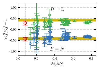
Figure 31: The same as Fig. 30 for the scalar channel. The yellow bands depict the $m_{s}=m_{\ell}=0$ predictions $\pm D_{S}(0)/F_{S}(0)$ obtained from the extrapolations of the individual charges.

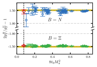
Figure 32: The same as Fig. 30 for the tensor channel.

Regarding the tensor charges we find in the $N_{f}=3$ $\overline{\text{MS}}$ scheme at $\mu=2\,\text{GeV}$

$$g_{T}^{N}=0.984^{(19)}_{(29)},\quad g_{T}^{\Sigma}=0.798^{(15)}_{(21)},\quad g_{T}^{\Xi}=-0.1872^{(59)}_{(41)}.$$ (45)

Since the anomalous dimension of the tensor bilinear is smaller than for the scalar case, we would expect no statistically relevant difference between the $N_{f}=3$ and $N_{f}=4$ schemes at $\mu=2\,\text{GeV}$. The nucleon charge agrees with the FLAG 21 [78] value of $g_{T}^{N}=0.965(61)$ [53] for $N_{f}=2+1$ and other recent lattice studies. These are shown in Fig. 29 along with determinations from phenomenology. The large uncertainties of the latter reflect the lack of experimental data. In particular, in Refs. [14, 15] the JAM collaboration constrain the first Mellin moment of the isovector combination of the transverse parton distribution functions to reproduce a lattice result for $g_{T}^{N}$. QCDSF-UKQCD-CSSM also determined the hyperon tensor charges [26]. Their results $g_{T}^{\Sigma}=0.805(15)_{\text{stat}}(02)_{\text{sys}}$ and $g_{T}^{\Xi}=-0.1952(74)_{\text{stat}}(10)_{\text{sys}}$ are in good agreement with ours.

V.2 SU(3) flavour symmetry breaking

On the SU(3) flavour symmetric line, i.e., for $m=m_{\ell}=m_{s}$, the baryon charges $g_{J}^{B}(m)$ can be decomposed into two functions, $F_{J}(m)$ and $D_{J}(m)$, see Sec. II and Eqs. (8)–(10). For the axial charges $g_{A}^{B}$, the values of these functions in the SU(3) chiral limit correspond to the LECs $F=F_{A}(0)$ and $D=D_{A}(0)$. We will not consider the vector channel ($J=V$) here since $F_{V}(m)=1$ and $D_{V}(m)=0$, which holds even at $m_{s}\neq m_{\ell}$, due to charge conservation.

Estimates of baryon structure observables often rely on SU(3) flavour symmetry arguments, however, it is not known a priori to what extent this symmetry is broken for $m_{s}\neq m_{\ell}$ and, in particular, at the physical point. Since within this analysis, we only determined three isovector charges ($B\in\{N,\Sigma,\Xi\}$) for each channel ($J\in\{A,S,T\}$), we cannot follow the systematic approach to investigate SU(3) flavour symmetry breaking of matrix elements proposed in Ref. [29]. Nevertheless, constructing appropriate ratios from the individual charges will provide us with estimates of the flavour symmetry breaking effects for each channel.

Using Eqs. (8)–(10), we obtain for $m=m_{s}=m_{\ell}$

$$\frac{2g_{J}^{B}(m)}{g_{J}^{\Sigma}(m)}-1=\pm\frac{D_{J}(m)}{F_{J}(m)},$$ (46)

where ‘$+$’ and ‘$-$’ corresponds to $B=N$ and $B=\Xi$, respectively. Figure 30 shows these combinations for the axial charges, as functions of the squared pion mass, compared to the chiral, continuum limit expectations $\pm D/F$ (yellow bands) determined from our global fit (see Fig. 18 and Table 13). The chiral limit value agrees with our earlier result $D/F=1.641^{(27)}_{(44)}$ [64] (model averaging recomputed for $D/F$ instead of $F/D$) within 1.5 standard errors. The data shown in the figure are not corrected for volume or lattice spacing effects. Note that the renormalization factors and improvement coefficients and, possibly, other systematics cancel from Eq. (46). For the ratio of the $\Xi$ over the $\Sigma$ axial charge we see no significant difference between the physical point value and that obtained for the same average quark mass at the flavour symmetric point. The symmetry breaking effect of the combination involving $g_{A}^{N}/g_{A}^{\Sigma}$ can be attributed to the pion mass dependence of $g_{A}^{N}$, see Fig. 17. The red symbols at the physical point (dashed vertical line) correspond to our continuum, infinite volume limit extrapolated results, listed in Table 13 for the combinations Eq. (46).

Table 13: The combinations $2g_{J}^{B}/g_{J}^{\Sigma}-1$ of Eq. (46) with $B\in\{N,\Xi\}$ at the physical point, in the continuum and infinite volume limit. These are computed from the individual charges in Tables 10 (for $Z_{A}^{3}$), 11 and 12 (for $Z_{J}^{1}$). The last row gives the combination $D_{J}(0)/F_{J}(0)$ in the chiral, continuum and infinite volume limit (yellow bands in Figs. 30–32), computed from the individual charges: $D_{J}/F_{J}=(g_{J}^{N}-g_{J}^{\Xi})/g_{J}^{\Sigma}$.

$B$	$2g_{A}^{B}/g_{A}^{\Sigma}-1$	$2g_{S}^{B}/g_{S}^{\Sigma}-1$	$2g_{T}^{B}/g_{T}^{\Sigma}-1$
$N$	$\phantom{-}1.93^{(12)}_{(15)}$	$-0.441^{(76)}_{(89)}$	$\phantom{-}1.467^{(67)}_{(99)}$
$\Xi$	$-1.609^{(37)}_{(40)}$	$\phantom{-}0.288^{(91)}_{(96)}$	$-1.469^{(17)}_{(16)}$
$D_{J}(0)/F_{J}(0)$	$\phantom{-}1.79^{(11)}_{(~{}8)}$	$-0.416^{(46)}_{(49)}$	$\phantom{-}1.530^{(54)}_{(56)}$

In Fig. 31 the combinations Eq. (46) are shown for the isovector scalar charges. These are compared to our SU(3) chiral limit extrapolated results (yellow bands) and the continuum, infinite volume limit results at the physical point (red diamonds). We find no statistically significant symmetry breaking in this case. However, the statistical errors are larger than for the axial case and also $F_{S}>F_{A}$. Therefore, we cannot exclude symmetry breaking of a similar size as for the axial charges, in particular, in the ratio of the $\Xi$ over the $\Sigma$ baryon charge. Finally, in Fig. 32 we carry out the same comparison for the tensor charges. In this case, within errors of a few per cent, no flavour symmetry violation is seen. Moreover, $D_{T}(m)/F_{T}(m)=D_{T}(0)/F_{T}(0)$ within errors.

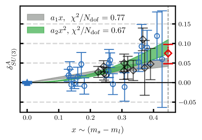
Figure 33: The SU(3) symmetry breaking ratio $\delta_{\text{SU(3)}}^{A}(x)$ (Eq. (48)) for the axial charges as a function of $x=(M_{K}^{2}-M_{\pi}^{2})/(2M_{K}^{2}+M_{\pi}^{2})$. Circles (diamonds) correspond to the $\operatorname{tr}M=\text{const.}$ ($m_{s}=\text{const.}$) trajectories, the triangle to $m_{s}=m_{\ell}$. The grey (green) band shows the result from a linear (quadratic) one parameter fit including only the blue data points that correspond to the ensembles on the $\operatorname{tr}\,M=\text{const.}$ line. Black data points correspond to ensembles on the $m_{s}=\text{const.}$ trajectory. The vertical grey dashed line indicates the physical point. The red diamond corresponds to the result derived from the values for the individual charges, see Sec. V.1.

In order to quantify the symmetry breaking effect between matrix elements involving the current $J$ as a function of the quark mass splitting $m_{s}-m_{\ell}$, we define

$$\delta_{\text{SU(3)}}^{J}=\frac{g_{J}^{\Xi}+g_{J}^{N}-g_{J}^{\Sigma}}{g_{J}^{\Xi}+g_{J}^{N}+g_{J}^{\Sigma}},$$ (47)

where for $m_{s}=m_{\ell}$, $\delta_{\text{SU(3)}}^{J}=(2F_{J}-2F_{J})/(2F_{J}+2F_{J})=0$, see Eqs. (8)–(10). Also from these ratios some of the systematics as well as the renormalization factors and improvement terms will cancel. We define a dimensionless SU(3) breaking parameter $x=(M_{K}^{2}-M_{\pi}^{2})/(2M_{K}^{2}+M_{\pi}^{2})\sim m_{s}-m_{\ell}$ and assume a polynomial dependence:

$$\delta^{J}_{\text{SU(3)}}=\sum_{n>0}a^{J}_{n}\,x^{n}.$$ (48)

The data for $\delta_{\text{SU(3)}}^{A}(x)$ depicted in Fig. 33 become more and more positive as the physical point (vertical dashed line) is approached. This observation agrees with findings from earlier studies [22, 23, 24, 25, 26]. We fit to data for which the average quark mass is kept constant (blue circles). However, there is no significant difference between these and the $m_{s}\approx\text{const}.$ points (black squares). Both linear and quadratic fits in $x$ ($a^{A}_{n}=0$ for $n\neq 1$ and $a^{A}_{n}=0$ for $n\neq 2$, respectively) give adequate descriptions of the data and agree with our continuum, infinite volume limit extrapolated physical point result (red diamond)

$$\delta^{A}_{\text{SU(3)}}=0.075^{(23)}_{(27)},$$ (49)

derived from the values for the individual charges. Effects of this sign and magnitude were also reported previously. ETMC [24] find $g_{A}^{N}+g_{A}^{\Xi}-g_{A}^{\Sigma}=0.147(24)$, whereas Savanur and Lin [25] quote $(g_{A}^{N}+g_{A}^{\Xi}-g_{A}^{\Sigma})/g_{A}^{N}=0.087(15)$.

For $J\neq A$ no statistically significant effects were observed. Nevertheless, for completeness we carry out the same analysis for $J=S$ and $J=T$, see Fig. III.1. Our continuum, infinite volume limit extrapolated physical point results

$$\delta^{S}_{\text{SU(3)}}=-0.040^{(37)}_{(41)},\quad\delta^{T}_{\text{SU(3)}}=-0.001^{(16)}_{(23)}$$ (50)

provide upper limits on the relative size of SU(3) flavour violation at the physical point.

Figure 34: The same as Fig. 33 for the scalar (top) and tensor (bottom) charges.

V.3 The up and down quark mass difference

Our results on the scalar charges, in particular, $g_{S}^{\Sigma}$, enable us to determine the quark mass splitting $\delta_{m}=m_{u}-m_{d}$. While we simulate the isosymmetric theory, in Nature this symmetry is broken. The extent of isospin symmetry breaking is determined by two small parameters, $\delta_{m}/\Lambda_{\text{QCD}}$ and the fine structure constant $\alpha_{\text{QED}}$, which are similar in size. The vector Ward identity relates $\delta_{m}$ to the QCD contributions to baryon mass splittings within an isomultiplet. In particular, to leading order in $\delta_{m}/\Lambda_{\text{QCD}}$ and $\alpha_{\text{QED}}$, the difference between the $\Sigma^{+}$ and $\Sigma^{-}$ baryon masses is a pure QCD effect from which, with our knowledge of $g_{S}^{\Sigma}$, we can extract $\delta_{m}$ without additional assumptions.

We consider isospin multiplets of baryons $B^{Q}\in\{N^{Q},\Sigma^{Q},\Xi^{Q}\}$ with electric charges $Q=I_{3}+\tfrac{1}{2}(1+S)\in\{0,\pm 1\}$ ($N^{+}=p$, $N^{0}=n$) and define the mass differences $\Delta m_{B^{Q+1}}=m_{B^{Q+1}}-m_{B^{Q}}$. Note that for the $\Sigma$ there are two differences [75],

$$\Delta m_{\Sigma^{+}} =m_{\Sigma^{+}}-m_{\Sigma^{0}}=-3.27(7)\,\text{MeV},$$ (51)

$$\Delta m_{\Sigma^{0}} =m_{\Sigma^{0}}-m_{\Sigma^{-}}=-4.81(4)\,\text{MeV}.$$ (52)

The other splittings read [75]

$$\Delta m_{\Xi}=-6.85(21)\,\text{MeV},\quad\Delta m_{N}\approx-1.293\,\text{MeV}.$$ (53)

The mass differences can be split into QCD ($\sim\delta_{m}$) and QED ($\sim\alpha_{\text{QED}}\Lambda_{\text{QCD}}$) contributions:

$$\Delta m_{B}=\Delta m_{B}^{\text{QCD}}+\Delta m_{B}^{\text{QED}}.$$ (54)

The splitting depends on the scale, the renormalization scheme and the matching conventions between QCD and QCD+QED. The Cottingham formula [118] relates the leading QED contribution to hadron masses to the total electric charge squared times a function of the unpolarized Compton forward-amplitude, i.e., to leading order in $\alpha_{\text{QED}}$ the electric contribution to charge-neutral hadron masses should vanish (as was suggested in the massless limit by Dashen [119]). Moreover, for $\delta_{m}=0$ this implies that the leading QED contributions to the masses of the $\Sigma^{+}$ and $\Sigma^{-}$ baryons are the same. Therefore, up to $\mathcal{O}(\alpha_{\text{QED}},\delta_{m}/\Lambda_{\text{QCD}})\cdot\delta_{m}$ terms,

$$\Delta m_{\Sigma}^{\text{QCD}} =\frac{1}{2}(m_{\Sigma^{+}}-m_{\Sigma^{-}})$$

$$=-4.04(4)\,\text{MeV},$$ (55)

$$\Delta m_{\Sigma^{+}}^{\text{QED}} =\frac{1}{2}(m_{\Sigma^{+}}+m_{\Sigma^{-}})-m_{\Sigma^{0}}$$

$$=0.77(5)\,\text{MeV}=-\Delta m_{\Sigma^{0}}^{\text{QED}}.$$ (56)

From the Ademollo-Gatto theorem [74] we know that the leading isospin breaking effects on the vector charges $g_{V}^{N}=g_{V}^{\Xi}=1$ and $g_{V}^{\Sigma}=2$ are quadratic functions of $\delta_{m}/\Lambda_{\text{QCD}}$ and $\alpha_{\text{QED}}$, whereas the scalar charges $g_{S}^{B}$ are subject to linear corrections in $\alpha_{\text{QED}}$ and $\delta_{m}/\Lambda_{\text{QCD}}$.

The Lorentz decomposition of the on-shell QCD matrix element for the isovector vector current between baryons $B^{\prime}=B^{Q+1}$ and $B=B^{Q}$ (that differ by $\Delta I_{3}=1$ in their isospin) gives (see Eq. (1))

$$i\partial^{\mu}\langle B^{\prime}(p^{\prime})| \bar{d}\gamma_{\mu}u|B(p)\rangle=g_{V}^{B^{\prime}B}i\partial^{\mu}\bar{u}_{B^{\prime}}(p^{\prime})\gamma_{\mu}u_{B}(p)$$

$$=g_{V}^{B^{\prime}B}\Delta m_{B}^{\text{QCD}}[1+\mathcal{O}(\delta_{m}/\Lambda_{\text{QCD}})],$$ (57)

where the leading correction is due to $q_{0}=p_{0}^{\prime}-p_{0}=\Delta m^{\text{QCD}}_{B}=|\mathbf{q}|$. In the last step we used the equations of motion. Combining this with the vector Ward identity $i\partial^{\mu}\bar{d}\gamma_{\mu}u=(m_{u}-m_{d})\bar{d}u$ gives

$$g_{V}^{B^{\prime}B}\Delta m^{\text{QCD}}_{B}=g_{S}^{B^{\prime}B}(m_{u}-m_{d})$$ (58)

as the QCD contribution to the mass difference, with corrections that are suppressed by powers of the symmetry breaking parameters. Note that the normalization convention of the charges $g_{J}^{B}$ defined in Eq. (3),

$$g_{J}^{pn}=g_{J}^{N},\quad g_{J}^{\Sigma^{+}\Sigma^{0}}=-g_{J}^{\Sigma}/\sqrt{2},\quad g_{J}^{\Xi^{0}\Xi^{-}}=-g_{J}^{\Xi},$$ (59)

cancels in the above equation so that we can replace $g_{J}^{B^{\prime}B}\mapsto g_{J}^{B}$ to obtain

$$\delta_{m}=m_{u}-m_{d}=\frac{g_{V}^{B}}{g_{S}^{B}}\Delta m^{\text{QCD}}_{B},$$ (60)

which we refer to as the CVC relation.

Using our physical point, continuum and infinite volume limit result $g_{S}^{\Sigma}=3.98^{(22)}_{(24)}$, assuming $g_{V}^{\Sigma}=2$ and applying Eq. (60) for the $\Sigma$ baryon, we obtain in the $N_{f}=3$ $\overline{\text{MS}}$ scheme at $\mu=2\,\text{GeV}$

$$m_{u}-m_{d}=-2.03^{(12)}_{(12)}\,\text{MeV}.$$ (61)

We expect $|\mathcal{O}(\delta_{m}/\Lambda_{\text{QCD}},\alpha_{\text{QED}})|\lesssim 1\%$ corrections from higher order effects to this result, which we can neglect at the present level of accuracy.

Table 14: Comparison of the light quark mass difference.

	$N_{f}$	$\delta_{m}$/MeV
RM123 [121]	2+1+1	$-2.38(18)$
FNAL-MILC [122]	2+1+1	$-2.55^{(9)}_{(7)}$
MILC [123]	2+1+1	$-2.57^{(11)}_{(6)}$
BMWc [116]	2+1	$-2.41(12)$
This work	2+1	$-2.03(12)$

We can compare our value of $\delta_{m}$ with results from the literature in Table 14. This includes the $N_{f}=2+1$ result of BMWc [116] and the $N_{f}=2+1+1$ continuum limit results of RM123 [121], FNAL-MILC [122] and MILC [123]. In the latter two cases we convert results for $m_{u}/m_{d}$ into $\delta_{m}$ as described in the table caption. We see a tension between the previous determinations and our result on the two to three $\sigma$ level.

We remark that all the previous results utilize the dependence of the pion and kaon masses on the quark masses and the electromagnetic coupling. We consider our method of determining the quark mass splitting from the scalar coupling $g^{\Sigma}_{S}$ and the mass difference between the $\Sigma^{+}$ and the $\Sigma^{-}$ baryons as more direct. In Ref. [124] $\Delta m_{N}^{\text{QCD}}=-1.87(16)\,\text{MeV}$ (which agrees within errors with lattice determinations, including ours, see below) is determined from experimental input. A larger (negative) QCD difference would require a larger QED contribution to the proton mass. As discussed above, the QED contribution to the mass of the $\Sigma^{+}$ baryon is $0.77(5)\,\text{MeV}$ (similar in size to $\Delta m_{N}^{\text{QED}}=0.58(16)\,\text{MeV}$ [124]) and it would be surprising if this increased when replacing a strange quark by a down quark. Assuming $\Delta m_{N}^{\text{QCD}}=-1.87(16)\,\text{MeV}$ and a value $\delta_{m}\approx-2.50(10)\,\text{MeV}$ as suggested by Refs. [116, 121, 122, 123] would require a coupling $g_{S}^{N}=0.75(7)$ to satisfy the CVC relation Eq. (60). This in turn is hard to reconcile with the majority of lattice results compiled in Fig. 28. With a lower value for $|\delta_{m}|$ (and/or a larger $|\Delta m_{N}^{\text{QCD}}|$) this inconsistency disappears.

V.4 QCD and QED isospin breaking effects on the baryon masses

We proceed to compute the QED contributions to the proton and $\Xi^{-}$ masses, $\Delta m_{N}^{\text{QED}}$ and $-\Delta m_{\Xi}^{\text{QED}}$:

$$\Delta m^{\text{QED}}_{N} =\Delta m_{N}-g_{S}^{N}(m_{u}-m_{d})$$

$$=\Delta m_{N}-\frac{2g_{S}^{N}}{g_{S}^{\Sigma}}\Delta m_{\Sigma}^{\text{QCD}},$$ (62)

$$\Delta m^{\text{QED}}_{\Xi} =\Delta m_{\Xi}-\frac{2g_{S}^{\Xi}}{g_{S}^{\Sigma}}\Delta m_{\Sigma}^{\text{QCD}}.$$ (63)

This gives

$$\Delta m_{N}^{\text{QED}} =0.97^{(31)}_{(36)}\,\text{MeV}, \!\!\!\!\Delta m_{N}^{\text{QCD}} =-2.26^{(31)}_{(36)}\,\text{MeV},$$ (64)

$$\Delta m_{\Sigma}^{\text{QED}} =0.77(05)\,\text{MeV}, \!\!\!\!\Delta m_{\Sigma}^{\text{QCD}} =-4.04(04)\,\text{MeV},$$ (65)

$$\Delta m_{\Xi}^{\text{QED}} =-1.65^{(37)}_{(39)}\,\text{MeV}, \!\!\!\!\Delta m_{\Xi}^{\text{QCD}} =-5.20^{(42)}_{(44)}\,\text{MeV}.$$ (66)

For completeness we included the values for the $\Sigma$ baryons that we determined from the experimental masses alone, without lattice input. The above mass splittings agree with the BMWc [117] continuum limit results from simulations of QCD plus QED, see Fig. 35 (errors added in quadrature). Nevertheless, as mentioned above, the value of $\delta_{m}$, reported by BMWc [116] from simulations of QCD with quenched QED, differs by 2.2 standard deviations from our result in Eq. (61). Also other lattice results on the QCD contribution to the mass-splittings (summarized in Fig. 35), obtained at a single lattice spacing from Endres et al. [125] using $\text{QED}_{\text{TL}}$ and $\text{QED}_{\text{M}}$, Brantley et al. [126] and CSSM-QCDSF-UKQCD [127] agree within errors.

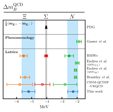
Figure 35: Comparison of the QCD contributions to isospin mass splittings [75, 117, 125, 126, 127, 124]. Note that in our normalization $m_{\Sigma^{+}}-m_{\Sigma^{-}}\approx 2\Delta m_{\Sigma}^{\text{QCD}}$. Values with filled symbols were obtained via a quark mass, continuum and finite volume extrapolation. Endres et al. [125] only quote values for $\Delta m_{N}^{\text{QED}}$ from which we compute $\Delta m_{N}^{\text{QCD}}$ employing the experimental proton-neutron mass splitting.

We mention the possibility of an enhancement of the (higher order) $\delta_{m}^{2}/\Lambda_{\text{QCD}}$ correction to the $\Sigma^{0}$ mass due to the possibility of mixing with the $\Lambda^{0}$, which, however, appears to be a very small effect [128]. A positive contribution to the $\Sigma^{0}$ mass would increase $\Delta m_{\Sigma}^{\text{QED}}$ but leave $\Delta m_{\Sigma}^{\text{QCD}}$ (and therefore the quark mass difference Eq. (61)) invariant.

The electromagnetic contributions to the $p$, $\Sigma^{\pm}$ and $\Xi^{-}$ masses are all similar to $1\,\text{MeV}$, with an enhancement for the heavier, more compact cascade baryon. Recently, combining the Cottingham formula [118] with experimental input from elastic scattering and parton distribution functions, the value $\Delta m_{N}^{\text{QED}}=0.58(16)\,\text{MeV}$ was determined in Ref. [124]. While within errors our result Eq. (64) agrees with this value, the number obtained in Ref. [124] is more inline with the suggested ordering $\Delta m_{N}^{\text{QED}}<\Delta m_{\Sigma}^{\text{QED}}<-\Delta m_{\Xi}^{\text{QED}}$. Combining their value with our determination of $g_{S}^{N}$ gives $\delta_{m}=-1.69^{(28)}_{(26)}\text{MeV}$, somewhat smaller in modulus than our result Eq. (61) and certainly in tension with, e.g., $\delta_{m}=-2.41(12)\,\text{MeV}$ [116].

We find that the effect of $m_{d}>m_{u}$ on the $\Xi$ and $\Sigma$ mass splittings is much bigger than for the nucleon since this is proportional to $g_{S}^{B}/g_{V}^{B}$ and $g_{S}^{N}<g_{S}^{\Sigma}/2<g_{S}^{\Xi}$. This hierarchy is due to $g_{S}^{N}\approx F_{S}+D_{S}$, $g_{S}^{\Sigma}/2\approx F_{S}$ and $g_{S}^{\Xi}\approx F_{S}-D_{S}$ with $F_{S}>0$ and $D_{S}<0$. Interestingly, the pion baryon $\sigma$ terms $\sigma_{\pi B}=\sigma_{uB}+\sigma_{dB}$ that encode the up plus down quark mass contribution to the baryon masses exhibit the opposite ordering [17], $\sigma_{\pi N}>\sigma_{\pi\Sigma}>\sigma_{\pi\Xi}$.

V.5 Isospin breaking effects on the pion baryon $\sigma$ terms

Having determined the quark mass differences, we can also compute the leading isospin violating corrections to the pion baryon $\sigma$ terms $\sigma_{\pi B}=\sigma_{uB}+\sigma_{dB}$. One can either work with matrix elements [129], using the identity

$$m_{u}\bar{u}u+m_{d}\bar{d}d=m_{\ell}\left(\bar{u}u+\bar{d}{d}\right)+\frac{\delta_{m}}{2}\left(\bar{u}u-\bar{d}d\right),$$ (67)

or one can start from the Feynman-Hellmann theorem

$$\sigma_{qB}=m_{q}\frac{\langle B|\bar{q}q|B\rangle}{\langle B|B\rangle}=m_{q}\frac{\partial m_{B}}{\partial m_{q}}.$$ (68)

Writing $m_{p}=m_{N}+\Delta m_{N}^{\text{QCD}}/2+\Delta m_{N}^{\text{QED}}$ and $m_{n}=m_{N}-\Delta m_{N}^{\text{QCD}}/2$, where $\Delta m_{N}^{\text{QCD}}=\delta_{m}g_{S}^{N}/g_{V}^{N}$, and realizing that the dependence of the QED contributions on the quark masses is of higher order in the isospin breaking, we obtain at linear order

$$\sigma_{\pi p} =m_{u}\frac{\partial m_{p}}{\partial m_{u}}+m_{d}\frac{\partial m_{p}}{\partial m_{d}}=\sigma_{\pi N}+\frac{1}{2}\Delta m_{N}^{\text{QCD}},$$ (69)

$$\sigma_{\pi n} =m_{u}\frac{\partial m_{n}}{\partial m_{u}}+m_{d}\frac{\partial m_{n}}{\partial m_{d}}=\sigma_{\pi N}-\frac{1}{2}\Delta m_{N}^{\text{QCD}}.$$ (70)

The same can be carried out for the $\Sigma^{\pm}$, $\Xi^{0}$ and $\Xi^{-}$ baryons. Using the results for the $\sigma$ terms of the isosymmetric theory of Ref. [17], we obtain

$$\sigma_{\pi p} =42.8^{(4.7)}_{(4.7)}\,\text{MeV}, \sigma_{\pi n} =45.0^{(4.7)}_{(4.7)}\,\text{MeV},$$ (71)

$$\sigma_{\pi\Sigma^{+}} =21.9^{(3.8)}_{(6.1)}\,\text{MeV}, \sigma_{\pi\Sigma^{-}} =29.9^{(3.8)}_{(6.1)}\,\text{MeV},$$ (72)

$$\sigma_{\pi\Xi^{0}} =8.6^{(4.5)}_{(6.4)}\,\text{MeV}, \sigma_{\pi\Xi^{-}} =13.8^{(4.5)}_{(6.4)}\,\text{MeV},$$ (73)

whereas the pion $\sigma$ term for the $\Sigma^{0}$ is not affected at linear order: $\sigma_{\pi\Sigma^{0}}\approx\sigma_{\pi\Sigma}=25.9^{(3.8)}_{(6.1)}\,\text{MeV}$. We refrain from further decomposing the pion baryon $\sigma$ terms into the individual up and down quark contributions. However, this can easily be accomplished [129]. It is worth noting that $(\sigma_{\pi\Xi^{-}}-\sigma_{\pi\Xi^{0}})/\sigma_{\pi\Xi}\gg(\sigma_{\pi n}-\sigma_{\pi p})/\sigma_{\pi N}$, in spite of the same isospin difference.

VI Summary and outlook

We determined the axial, scalar and tensor isovector charges of the nucleon, sigma and cascade baryons using $N_{f}=2+1$ lattice QCD simulations. The analysis is based on 47 gauge ensembles, spanning a range of pion masses from $430\,\text{MeV}$ down to a near physical value of $130\,\text{MeV}$ across six different lattice spacings between $a\approx 0.039\,\text{fm}$ and $a\approx 0.098\,\text{fm}$ and linear spatial lattice extents $3.0\,M_{\pi}^{-1}\leq L\leq 6.5\,M_{\pi}^{-1}$. The availability of ensembles lying on three trajectories in the quark mass plane enables SU(3) flavour symmetry breaking to be explored systematically and the quark mass dependence of the charges to be tightly constrained. Simultaneous extrapolations to the physical point in the continuum and infinite volume limit are performed. Systematic errors are assessed by imposing cuts on the pion mass, the lattice spacing and the volume as well as using different sets of renormalization factors. Our results (in the $\overline{\text{MS}}$ scheme at $\mu=2\,\text{GeV}$) for the nucleon charges are

$$g_{A}^{N} =1.284^{(28)}_{(27)}, g_{S}^{N} =1.11^{(14)}_{(16)}, g_{T}^{N} =0.984^{(19)}_{(29)}.$$

For the hyperon charges we find

$$g_{A}^{\Sigma} =0.875^{(30)}_{(39)}, g_{S}^{\Sigma} =3.98^{(22)}_{(24)}, g_{T}^{\Sigma} =0.798^{(15)}_{(21)},$$

$$g_{A}^{\Xi} =-0.267^{(13)}_{(12)}, g_{S}^{\Xi} =2.57^{(11)}_{(11)}, g_{T}^{\Xi} =-0.1872^{(59)}_{(41)}.$$

A comparison with previous works is presented in Sec. V.1. We quantify SU(3) symmetry breaking effects for the axial charge at the physical point in terms of the combination

$$\delta^{A}_{\text{SU(3)}}=\frac{g_{A}^{\Xi}+g_{A}^{N}-g_{A}^{\Sigma}}{g_{A}^{\Xi}+g_{A}^{N}+g_{A}^{\Sigma}}=0.075^{(23)}_{(27)},$$

see Fig. 33. In particular the axial charge of the nucleon deviates from its value in the SU(3) chiral limit, as can be seen in Fig. 30 and Table 13. No significant symmetry breaking is observed for the other charges within current precision, see Figs. 31, 32 and III.1.

To cross-check the analysis methods, the vector charges are determined and the expected values, $g_{V}^{N}=g_{V}^{\Xi}=1$ and $g_{V}^{\Sigma}=2$, are reproduced reasonably well:

$$g_{V}^{N} =1.0012^{(12)}_{(11)}, g_{V}^{\Sigma} =2.021^{(21)}_{(27)}, g_{V}^{\Xi} =1.015^{(10)}_{(11)}.$$

Furthermore, we exploit the conserved vector current relation to predict the quark mass difference

$$m_{u}-m_{d}=-2.03(12)\,\text{MeV}$$

from the scalar charge of the $\Sigma$ baryon. We utilize this to decompose isospin mass splittings between the baryons into QCD and QED contributions (see Eqs. (64)–(66)) and to predict the leading isospin corrections to the pion baryon $\sigma$ terms (see Eqs. (71)–(73)).

A computationally efficient stochastic approach was employed in the analysis, which allows for the simultaneous evaluation of the three-point correlation functions of all baryons with a variety of current insertions and momentum combinations. This work is a first step towards determining hyperon decay form factors which are relevant for the study of CP violation [130]. A complementary study of the baryon octet $\sigma$ terms on the same data set as used here is already ongoing [131].

Appendix A Further details of the three-point function measurements

A.1 Comparison of the stochastic and sequential source methods

We computed the connected three-point functions for all the octet baryons utilizing the computationally efficient stochastic approach outlined in Sec. III.3. This approach introduces additional stochastic noise on top of the gauge noise. In the analysis presented, for the nucleon, we make use of statistically more precise three-point correlation function measurements determined via the sequential source method as part of other projects. In the following, we compare the computational costs of the stochastic and the sequential source methods and the results for the ratios of the three-point over two-point functions for the nucleon.

As a typical example, we consider the measurements performed on ensemble N200 ($M_{\pi}=286$ MeV and $a=0.064$ fm). For our set-up, illustrated in Figs. 6 and 7, a total of $4\times 12$ solves are needed for the 4 source positions of the point-to-all propagators. To form the three-point functions for the nucleon an additional $N_{\text{sto}}=100$ light stochastic solves (for the timeslice-to-all propagators connecting the sink and current timeslices, the wiggly line in Fig. 6) are performed. This set-up provides 8 measurements of the nucleon three-point function (as shown in Fig. 7, with the source-sink separations $t/a=11$, $14$, $16$, $19$) and includes all polarizations (and the unpolarized case) as well as a range of sink momenta (almost) for free. In principle, decuplet baryon three-point functions can also be constructed at the analysis stage. This set-up is evaluated twice on each configuration leading to a total of 296 inversions. Similarly, an additional $(4\times 12+100)\times 2$ strange solves are performed in order to form the three-point functions for all the (octet and decuplet) hyperons, including strangeness changing currents that we did not consider here.

In the sequential source set-up, we compute the three-point function for the nucleon at rest, again for source-sink separations $t/a=11$, $14$, $16$ and $19$. Ten measurements are carried out per configuration (corresponding to 1, 2, 3 and 4 measurements for each $t$, respectively), where in each case the two light quark flavours ($u$ and $d$) of the current and the four possible polarizations of the nucleon require $2\times 4$ sequential sources to be constructed. This amounts to performing $(4+10\times 2\times 4)\times 12=1008$ light solves. The additional $4\times 12$ inversions refer to the point-to-all propagators for 4 different source positions that connect the source to the sink (and the current). This is three-times the cost of the stochastic approach (for the nucleon three-point functions), which realizes a range of sink momenta.

The ratios of the three-point over two-point functions for the nucleon obtained from the two different approaches are compared in Fig. III.1. A significant part of the gauge noise cancels in the ratio, while the (additional) stochastic noise remains. For our set-up, this leads to larger statistical errors for the stochastic data compared to the sequential source results. This difference can clearly be seen for the ratio in the vector channel, for which the gauge noise is minimal, however, the difference is less pronounced for the other charges. For the sigma and cascade baryons we generally find a good statistical signal in the ratios employing the stochastic approach, see Fig. 37, although, also in this case the ratios for the hyperon vector charges suffer from large errors.

Figure 36: Unrenormalized ratio of three-point over two-point functions for the nucleon vector, axial, scalar and tensor charge (from top to bottom) on ensemble N200. The left hand side shows the data from the sequential source method from 1,2,3 and 4 measurements (for increasing values of $t$) compared to the same measurements obtained from the stochastic approach with four measurements for each value of $t$ on the right hand side.

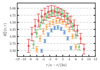
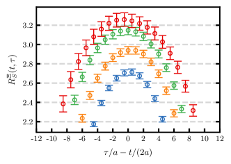
Figure 37: Unrenormalized ratio of three-point over two-point functions for the $\Sigma$ (left) and $\Xi$ (right) scalar charge on ensemble N200.

In the case of a large-scale analysis effort including high statistics, as presented in this article, the disk space required to store the stochastic three-point function data is significant. The individual spectator ($S$) and insertion ($I$) parts as defined in Eqs. (25) and (26), respectively, are stored with all indices open. In general this amounts to $N=N[S]+N[I]$ complex double precision floating point numbers for each gauge field configuration where

$$N[S] =N_{F}^{S}\cdot N_{\mathbf{p}^{\prime}}\cdot N_{\text{snk}}\cdot N_{\text{src}}\cdot N_{\text{sto}}\cdot N_{c}\cdot N_{s}^{5}\ ,$$ (74)

$$N[I] =N_{F}^{I}\cdot N_{\mathbf{q}}\cdot N_{\partial_{\mu}}\cdot N_{\tau}\cdot N_{\text{src}}\cdot N_{\text{sto}}\cdot N_{c}\cdot N_{s}^{2}\ .$$ (75)

Here $N_{F}^{S/I}$ denotes the number of flavour combinations for the spectator and insertion parts (typically 4 and 2, respectively), $N_{\mathbf{p}}$ gives the number of momentum combinations for a maximum momentum $|\mathbf{p}|$ (with $\mathbf{p}$ either being the sink momentum $\mathbf{p}^{\prime}$ or the momentum transfer $\mathbf{q}$), $N_{\text{src}/\text{snk}}$ corresponds to the number of source (4) and sink (2) positions, $N_{c}=3$ and $N_{s}=4$ are the dimensions of colour and spin space and $N_{\tau}$ is the number of current insertion timeslices, usually the distance between the two sink timeslices, see Figs. 6 and 7. $N_{\partial_{\mu}}$ refers to the number of derivatives included in the current insertion. We consider all currents including up to one derivative ($N_{\partial_{\mu}}=1+4$), although only the currents without derivatives are presented in this work. This adds up to a file size of the order of GBs for a single gauge field configuration and disk space usage of the order of TBs for a typical CLS gauge ensemble. Storing the data with all indices open allows for a very flexible analysis. Octet or decuplet baryon three-point functions can be constructed from the spectator and insertion parts for different polarizations, current insertions as well as for a large number of momentum combinations.

A.2 Treatment of outliers

When analysing the three-point functions on some of the ensembles, we observe a small number of three-point function results that are by many orders of magnitude larger than the rest. These outliers, whose origin currently remains unexplained, would have a significant impact on the analysis, as illustrated in Fig. 38 for ensemble D200 ($M_{\pi}=202$ MeV and $a=0.064$ fm). The three-point function for the scalar charge with source-sink separation $t/a=16$ for a single source position is displayed. In this case one outlier is identified (according to the criterion given below) and one sees a substantial change in the configuration average and a reduction in the standard deviation if this measurement (on a particular configuration) is excluded. The Mainz group [141] reported similar outliers when determining the nucleon $\sigma$ terms on a subset of the CLS gauge ensembles employed here. We remark that such outliers do not seem to occur in the distributions of the two-point function measurements.

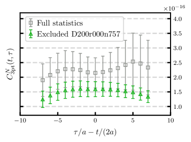
Figure 38: Nucleon three-point function for the scalar channel with a source-sink separation $t/a=16$ for a single source position on ensemble D200. The average and standard error is computed including and excluding one particular gauge configuration.

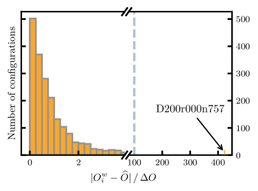
Figure 39: The numbers of configurations separated by a distance $|O_{i}^{w}-\widehat{O}|/\Delta O$ from the central value $\widehat{O}$ for the three-point function data of Fig. 38 on the insertion timeslice $\tau/a=15$. The blue dashed line indicates the cutoff $K=100$, which is exceeded by a single measurement. Note the cut and different scales of the ordinate. Due to this representation a few histogram entries are not shown.

To overcome this obstacle we constrain the analysed data and discard ‘outlier’ configurations on which measurements give contributions that are very far away from the expected central value. As discussed in Sec. III.1 we employ the appropriate reweighting factors where $w_{i}=w_{i}^{\ell}w_{i}^{s}$ is the product of the light and strange reweighting factors, determined on each configuration $i$, see in particular the discussion in Appendix G.2 of Ref. [17]. In order to have a robust estimate for the variance of the reweighted data

$$O_{i}^{w}=\frac{w_{i}O_{i}}{w},$$ (76)

where $w=N_{\text{cnfg}}^{-1}\sum_{i}w_{i}$, we determine the lower and upper boundary values $O^{w}_{\text{low}}$ and $O^{w}_{\text{up}}$ of the central 68% interval of this distribution. We then remove configurations $i$ with

$$|O_{i}^{w}-\widehat{O}|>K\,\Delta O,$$ (77)

where

$$\widehat{O}=\frac{O^{w}_{\text{up}}+O^{w}_{\text{low}}}{2},\quad\Delta O=\frac{O^{w}_{\text{up}}-O^{w}_{\text{low}}}{2},$$ (78)

setting the cutoff $K$ to a large value ($K=100$). In Fig. 39 we show the distribution of the measurements for the nucleon three-point function for a scalar current (at a single source position and current insertion time) on the ensemble D200 discussed above (see Fig. 38). The outlier is more than $400\,\Delta O$ away from $\widehat{O}$. Considering all the three-point function measurements across the different ensembles, we uniformly set the cutoff in Eq. (77) to $K=100$ and remove all configurations from the analysis on which at least one measurement satisfies this criterion.

Appendix B Additional tables

In Table B we include further details on the gauge ensembles. In Tables B–B the results for the unrenormalized charges for the three octet baryons are collected.

Table 15: The gauge ensembles utilized in this work: the light and strange hopping parameters $\kappa_{\ell}$ and $\kappa_{s}$, the gradient flow scale parameter $t_{0}/a^{2}$ and the pion ($M_{\pi}$) and kaon masses ($M_{K}$) [17].

Table 16: Results for the unrenormalized nucleon charges $g_{J}^{N,\text{latt}}$ for $J\in\{A,S,T,V\}$. #ES labels the number of excited states used to determine the ground state matrix element, see the discussion in Sec. III.4.

Table 17: Results for the unrenormalized hyperon charges $g_{J}^{\Sigma,\text{latt}}$ for $J\in\{A,S,T,V\}$. #ES labels the number of excited states used to determine the ground state matrix element, see the discussion in Sec. III.4. The three-point functions are computed employing the “stochastic” approach.

Table 18: Results for the unrenormalized hyperon charges $g_{J}^{\Xi,\text{latt}}$ for $J\in\{A,S,T,V\}$. #ES labels the number of excited states used to determine the ground state matrix element, see the discussion in Sec. III.4. The three-point functions are computed employing the “stochastic” approach.

Appendix C Additional figures

We provide additional figures (Figs. 40–47).

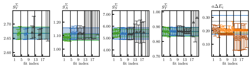
Figure 40: The same as Fig. III.1 for the sigma baryon.

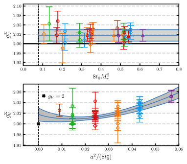
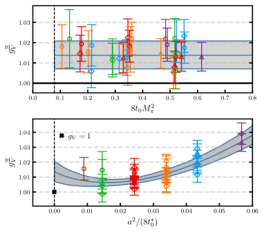
Figure 41: The same as Fig. 13 for the isovector vector charges $g_{V}^{B}$ of the sigma baryon (left) and the cascade baryon (right). For better visibility, the data points for ensemble D451, which have large errors (see Tables B and B), are not displayed. See Tables B and B for the set of ensembles used.

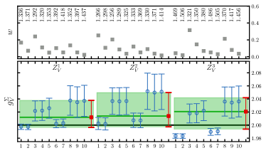
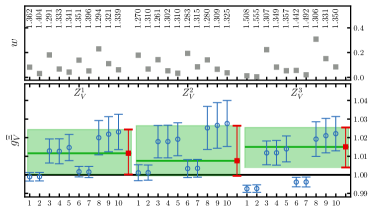
Figure 42: The same as Fig. 15 for the vector charge $g_{V}^{B}$ of the sigma (right) and cascade (left) baryon.

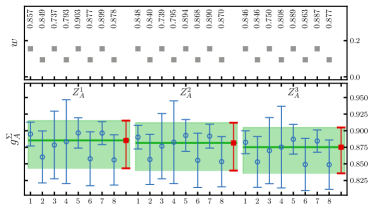
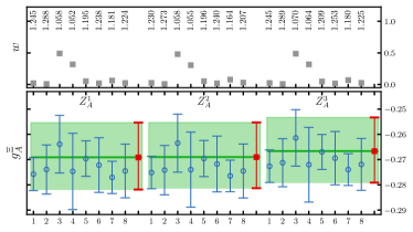
Figure 43: The same as Fig. 19 for the axial charge $g_{A}^{B}$ of the sigma (right) and cascade (left) baryon.

Figure 44: The same as Fig. 19 for the scalar charge $g_{S}^{B}$ of the nucleon (top, left), sigma (top, right) and cascade (bottom) baryons. The six fits correspond to two fit variations, see the text, applied to three data sets, DS($M_{\pi}^{\footnotesize{<400\,\text{MeV}}}$), DS($M_{\pi}^{\footnotesize{<400\,\text{MeV}}}$, $a^{\footnotesize{<0.1\,\text{fm}}}$) and DS($M_{\pi}^{\footnotesize{<400\,\text{MeV}}}$, $LM_{\pi}^{\footnotesize{>4}}$). The data are extracted using two excited states in the fitting analysis, see Sec. III.4. Only two different sets of renormalization factors are used.

Figure 45: The same as Fig. 19 for the tensor charge $g_{T}^{B}$ for the nucleon (top, left), sigma (top, right) and cascade (bottom) baryons. The data are extracted using two excited states in the fitting analysis, see Sec. III.4. Only two different sets of renormalization factors are used.

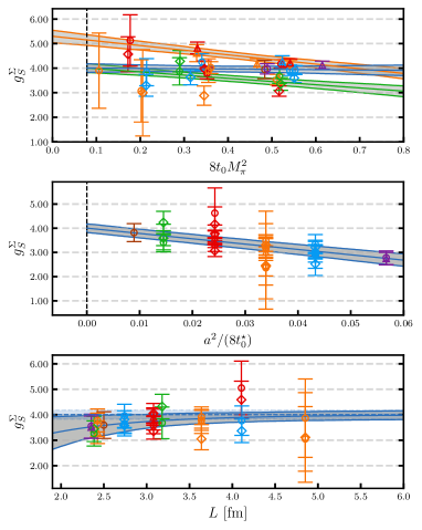
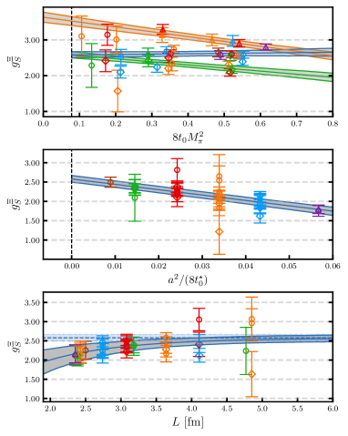
Figure 46: The same as Fig. 21 for the isovector scalar charges $g_{S}^{B}$ of the sigma baryon (left) and the cascade baryon (right). For better visibility, the data point for ensemble E300, which has a relatively large error (see Table B), is not displayed for the sigma baryon. See Tables B and B for the set of ensembles used.

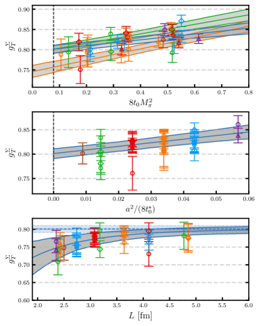
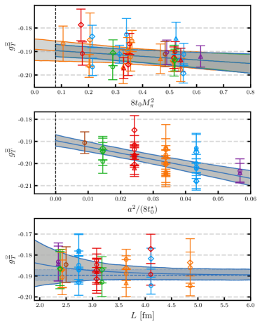
Figure 47: The same as Fig. 23 for the isovector tensor charges $g_{T}^{B}$ of the sigma baryon (left) and the cascade baryon (right). For better visibility, the data point for ensemble E300, which has a relatively large error (see Table B), is not displayed for the cascade baryon. See Tables B and B for the set of ensembles used.

References

- Ji [1997] X.-D. Ji, Gauge-invariant decomposition of nucleon spin, Phys. Rev. Lett. 78, 610 (1997), arXiv:hep-ph/9603249 .
- Jaffe and Manohar [1990] R. L. Jaffe and A. Manohar, The problem: Fact and fantasy on the spin of the proton, Nucl. Phys. B 337, 509 (1990).
- Bali et al. [2012] G. S. Bali et al. (QCDSF Collaboration), Strangeness contribution to the proton spin from lattice QCD, Phys. Rev. Lett. 108, 222001 (2012), arXiv:1112.3354 [hep-lat] .
- Engelhardt [2012] M. Engelhardt, Strange quark contributions to nucleon mass and spin from lattice QCD, Phys. Rev. D 86, 114510 (2012), arXiv:1210.0025 [hep-lat] .
- Gong et al. [2017] M. Gong, Y.-B. Yang, J. Liang, A. Alexandru, T. Draper, and K.-F. Liu (QCD Collaboration), Strange and charm quark spins from the anomalous Ward identity, Phys. Rev. D 95, 114509 (2017), arXiv:1511.03671 [hep-ph] .
- Alexandrou et al. [2017] C. Alexandrou, M. Constantinou, K. Hadjiyiannakou, K. Jansen, C. Kallidonis, G. Koutsou, A. Vaquero Avilés-Casco, and C. Wiese (ETM Collaboration), Nucleon spin and momentum decomposition using lattice QCD simulations, Phys. Rev. Lett. 119, 142002 (2017), arXiv:1706.02973 [hep-lat] .
- Green et al. [2017] J. Green, N. Hasan, S. Meinel, M. Engelhardt, S. Krieg, J. Laeuchli, J. Negele, K. Orginos, A. Pochinsky, and S. Syritsyn, Up, down, and strange nucleon axial form factors from lattice QCD, Phys. Rev. D 95, 114502 (2017), arXiv:1703.06703 [hep-lat] .
- Bürger et al. [2022] S. Bürger, T. Wurm, M. Löffler, M. Göckeler, G. Bali, S. Collins, A. Schäfer, and A. Sternbeck (RQCD Collaboration), Lattice results for the longitudinal spin structure and color forces on quarks in a nucleon, Phys. Rev. D 105, 054504 (2022), arXiv:2111.08306 [hep-lat] .
- de Florian et al. [2008] D. de Florian, R. Sassot, M. Stratmann, and W. Vogelsang, Global analysis of helicity parton densities and their uncertainties, Phys. Rev. Lett. 101, 072001 (2008), arXiv:0804.0422 [hep-ph] .
- Blümlein and Böttcher [2010] J. Blümlein and H. Böttcher, QCD analysis of polarized deep inelastic scattering data, Nucl. Phys. B 841, 205 (2010), arXiv:1005.3113 [hep-ph] .
- Nocera et al. [2014] E. R. Nocera, R. D. Ball, S. Forte, G. Ridolfi, and J. Rojo (NNPDF Collaboration), A first unbiased global determination of polarized PDFs and their uncertainties, Nucl. Phys. B 887, 276 (2014), arXiv:1406.5539 [hep-ph] .
- Sato et al. [2016] N. Sato, W. Melnitchouk, S. E. Kuhn, J. J. Ethier, and A. Accardi (JAM Collaboration), Iterative Monte Carlo analysis of spin-dependent parton distributions, Phys. Rev. D 93, 074005 (2016), arXiv:1601.07782 [hep-ph] .
- Ethier et al. [2017] J. J. Ethier, N. Sato, and W. Melnitchouk (JAM Collaboration), First simultaneous extraction of spin-dependent parton distributions and fragmentation functions from a global QCD analysis, Phys. Rev. Lett. 119, 132001 (2017), arXiv:1705.05889 [hep-ph] .
- Lin et al. [2018] H.-W. Lin, W. Melnitchouk, A. Prokudin, N. Sato, and H. Shows (JAM Collaboration), First Monte Carlo global analysis of nucleon transversity with lattice QCD Constraints, Phys. Rev. Lett. 120, 152502 (2018), arXiv:1710.09858 [hep-ph] .
- Gamberg et al. [2022] L. Gamberg, M. Malda, J. A. Miller, D. Pitonyak, A. Prokudin, and N. Sato (JAM Collaboration), Updated QCD global analysis of single transverse-spin asymmetries: Extracting , and the role of the Soffer bound and lattice QCD, Phys. Rev. D 106, 034014 (2022), arXiv:2205.00999 [hep-ph] .
- Bhattacharya et al. [2012] T. Bhattacharya, V. Cirigliano, S. D. Cohen, A. Filipuzzi, M. Gonzalez-Alonso, M. L. Graesser, R. Gupta, and H.-W. Lin, Probing novel scalar and tensor interactions from (ultra)cold neutrons to the LHC, Phys. Rev. D 85, 054512 (2012), arXiv:1110.6448 [hep-ph] .
- Bali et al. [2023a] G. S. Bali, S. Collins, P. Georg, D. Jenkins, P. Korcyl, A. Schäfer, E. E. Scholz, J. Simeth, W. Söldner, and S. Weishäupl (RQCD Collaboration), Scale setting and the light baryon spectrum in QCD with Wilson fermions, J. High Energy Phys. 05, 035 (2023a), arXiv:2211.03744 [hep-lat] .
- Leutwyler [2015] H. Leutwyler, Theoretical aspects of Chiral Dynamics, Proc. Sci. CD15, 022 (2015), arXiv:1510.07511 [hep-ph] .
- Fucito et al. [1982] F. Fucito, G. Parisi, and S. Petrarca, First evaluation of in lattice QCD in the quenched approximation, Phys. Lett. B 115, 148 (1982).
- Güsken et al. [1989] S. Güsken, U. Löw, K.-H. Mütter, R. Sommer, A. Patel, and K. Schilling, Nonsinglet axial vector couplings of the baryon octet in lattice QCD, Phys. Lett. B 227, 266 (1989).
- Woloshyn and Liu [1989] R. M. Woloshyn and K.-F. Liu, A study of the nucleon axial current coupling in quenched lattice QCD, Nucl. Phys. B 311, 527 (1989).
- Lin and Orginos [2009] H.-W. Lin and K. Orginos, First calculation of hyperon axial couplings from lattice QCD, Phys. Rev. D 79, 034507 (2009), arXiv:0712.1214 [hep-lat] .
- Erkol et al. [2010] G. Erkol, M. Oka, and T. T. Takahashi, Axial charges of octet baryons in two-flavor lattice QCD, Phys. Lett. B 686, 36 (2010), arXiv:0911.2447 [hep-lat] .
- Alexandrou et al. [2016] C. Alexandrou, K. Hadjiyiannakou, and C. Kallidonis (ETM Collaboration), Axial charges of hyperons and charmed baryons using twisted mass fermions, Phys. Rev. D 94, 034502 (2016), arXiv:1606.01650 [hep-lat] .
- Savanur and Lin [2020] A. Savanur and H.-W. Lin, Lattice-QCD determination of the hyperon axial couplings in the continuum limit, Phys. Rev. D 102, 014501 (2020), arXiv:1901.00018 [hep-lat] .
- Smail et al. [2023] R. E. Smail et al. (QCDSF-UKQCD-CSSM Collaboration), Constraining beyond the Standard Model nucleon isovector charges, (2023), arXiv:2304.02866 [hep-lat] .
- Borasoy and Meissner [1997] B. Borasoy and U.-G. Meissner, Chiral expansion of baryon masses and -terms, Ann. Phys. (N.Y.) 254, 192 (1997), arXiv:hep-ph/9607432 .
- Cooke et al. [2012] A. N. Cooke, R. Horsley, Y. Nakamura, D. Pleiter, P. E. L. Rakow, G. Schierholz, and J. M. Zanotti, The effects of flavour symmetry breaking on hadron matrix elements, Proceedings, 30th International Symposium on Lattice Field Theory (Lattice 2012): Cairns, Australia, June 24-29, 2012, Proc. Sci. LATTICE2012, 116 (2012), arXiv:1212.2564 [hep-lat] .
- Bickerton et al. [2019] J. M. Bickerton, R. Horsley, Y. Nakamura, H. Perlt, D. Pleiter, P. E. L. Rakow, G. Schierholz, H. Stüben, R. D. Young, and J. M. Zanotti (QCDSF-UKQCD-CSSM Collaboration), Patterns of flavor symmetry breaking in hadron matrix elements involving , , and quarks, Phys. Rev. D 100, 114516 (2019), arXiv:1909.02521 [hep-lat] .
- Jenkins and Manohar [1991a] E. E. Jenkins and A. V. Manohar, Chiral corrections to the baryon axial currents, Phys. Lett. B 259, 353 (1991a).
- Dashen and Manohar [1993] R. F. Dashen and A. V. Manohar, corrections to the baryon axial currents in QCD, Phys. Lett. B 315, 438 (1993), arXiv:hep-ph/9307242 .
- Bruno et al. [2015] M. Bruno et al. (CLS Effort), Simulation of QCD with flavors of non-perturbatively improved Wilson fermions, J. High Energy Phys. 02, 043 (2015), arXiv:1411.3982 [hep-lat] .
- Lüscher and Schaefer [2011] M. Lüscher and S. Schaefer, Lattice QCD without topology barriers, J. High Energy Phys. 07, 036, arXiv:1105.4749 [hep-lat] .
- Schaefer et al. [2011] S. Schaefer, R. Sommer, and F. Virotta (ALPHA Collaboration), Critical slowing down and error analysis in lattice QCD simulations, Nucl. Phys. B 845, 93 (2011), arXiv:1009.5228 [hep-lat] .
- Lüscher and Schaefer [2013] M. Lüscher and S. Schaefer, Lattice QCD with open boundary conditions and twisted-mass reweighting, Comput. Phys. Commun. 184, 519 (2013), arXiv:1206.2809 [hep-lat] .
- Clark and Kennedy [2007] M. A. Clark and A. D. Kennedy, Accelerating dynamical fermion computations using the rational hybrid Monte Carlo (RHMC) algorithm with multiple pseudofermion fields, Phys. Rev. Lett. 98, 051601 (2007), arXiv:hep-lat/0608015 .
- Mohler and Schaefer [2020] D. Mohler and S. Schaefer, Remarks on strange-quark simulations with Wilson fermions, Phys. Rev. D 102, 074506 (2020), arXiv:2003.13359 [hep-lat] .
- Bali et al. [2016] G. S. Bali, E. E. Scholz, J. Simeth, and W. Söldner (RQCD Collaboration), Lattice simulations with improved Wilson fermions at a fixed strange quark mass, Phys. Rev. D 94, 074501 (2016), arXiv:1606.09039 [hep-lat] .
- Nakamura and Stüben [2010] Y. Nakamura and H. Stüben, BQCD - Berlin quantum chromodynamics program, Proceedings, 28th International Symposium on Lattice Field Theory (Lattice 2010): Villasimius, Italy, June 14-19, 2010, Proc. Sci. LATTICE2010, 040 (2010), arXiv:1011.0199 [hep-lat] .
- Falcioni et al. [1985] M. Falcioni, M. L. Paciello, G. Parisi, and B. Taglienti (APE Collaboration), Again on SU(3) glueball mass, Nucl. Phys. B251, 624 (1985).
- Maiani et al. [1987] L. Maiani, G. Martinelli, M. L. Paciello, and B. Taglienti, Scalar densities and baryon mass differences in lattice QCD with Wilson fermions, Nucl. Phys. B293, 420 (1987).
- Bratt et al. [2010] J. D. Bratt et al. (LHP Collaboration), Nucleon structure from mixed action calculations using flavors of asqtad sea and domain wall valence fermions, Phys. Rev. D 82, 094502 (2010), arXiv:1001.3620 [hep-lat] .
- Bali et al. [2020] G. S. Bali, L. Barca, S. Collins, M. Gruber, M. Löffler, A. Schäfer, W. Söldner, P. Wein, S. Weishäupl, and T. Wurm (RQCD Collaboration), Nucleon axial structure from lattice QCD, J. High Energy Phys. 05, 126 (2020), arXiv:1911.13150 [hep-lat] .
- Evans et al. [2010] R. Evans, G. Bali, and S. Collins, Improved semileptonic form factor calculations in lattice QCD, Phys. Rev. D 82, 094501 (2010), arXiv:1008.3293 [hep-lat] .
- Bali et al. [2014] G. S. Bali, S. Collins, B. Gläßle, M. Göckeler, J. Najjar, R. Rödl, A. Schäfer, A. Sternbeck, and W. Söldner, Nucleon structure from stochastic estimators, Proceedings, 31st International Symposium on Lattice Field Theory (Lattice 2013): Mainz, Germany, July 29-August 3, 2013, Proc. Sci. LATTICE2013, 271 (2014), arXiv:1311.1718 [hep-lat] .
- Bali et al. [2019] G. S. Bali, S. Collins, P. Korcyl, R. Rödl, S. Weishäupl, and T. Wurm, Hyperon couplings from lattice QCD, Proc. Sci. LATTICE2019, 099 (2019), arXiv:1907.13454 [hep-lat] .
- Bali et al. [2018] G. S. Bali, S. Collins, B. Gläßle, S. Heybrock, P. Korcyl, M. Löffler, R. Rödl, and A. Schäfer, Baryonic and mesonic 3-point functions with open spin indices, Proceedings, 35th International Symposium on Lattice Field Theory (Lattice 2017): Granada, Spain, June 18-24, 2017, EPJ Web Conf. 175, 06014 (2018), arXiv:1711.02384 [hep-lat] .
- Löffler et al. [2022] M. Löffler, P. Wein, T. Wurm, S. Weishäupl, D. Jenkins, R. Rödl, A. Schäfer, and L. Walter (RQCD Collaboration), Mellin moments of spin dependent and independent PDFs of the pion and rho meson, Phys. Rev. D 105, 014505 (2022), arXiv:2108.07544 [hep-lat] .
- Alexandrou et al. [2014a] C. Alexandrou, S. Dinter, V. Drach, K. Jansen, K. Hadjiyiannakou, and D. B. Renner (ETM Collaboration), A stochastic method for computing hadronic matrix elements, Eur. Phys. J. C 74, 2692 (2014a), arXiv:1302.2608 [hep-lat] .
- Yang et al. [2016] Y.-B. Yang, A. Alexandru, T. Draper, M. Gong, and K.-F. Liu (QCD Collaboration), Stochastic method with low mode substitution for nucleon isovector matrix elements, Phys. Rev. D 93, 034503 (2016), arXiv:1509.04616 [hep-lat] .
- Dong and Liu [1994] S.-J. Dong and K.-F. Liu, Stochastic estimation with Z(2) noise, Phys. Lett. B 328, 130 (1994), arXiv:hep-lat/9308015 .
- Bernardson et al. [1993] S. Bernardson, P. McCarty, and C. Thron, Monte Carlo methods for estimating linear combinations of inverse matrix entries in lattice QCD, Comput. Phys. Commun. 78, 256 (1993).
- Harris et al. [2019] T. Harris, G. von Hippel, P. Junnarkar, H. B. Meyer, K. Ottnad, J. Wilhelm, H. Wittig, and L. Wrang, Nucleon isovector charges and twist-2 matrix elements with dynamical Wilson quarks, Phys. Rev. D 100, 034513 (2019), arXiv:1905.01291 [hep-lat] .
- Korcyl and Bali [2016] P. Korcyl and G. S. Bali, Non-perturbative determination of improvement coefficients using coordinate space correlators in lattice QCD, Proceedings, 34th International Symposium on Lattice Field Theory (Lattice 2016): Southampton, UK, July 24-30, 2016, Proc. Sci. LATTICE2016, 190 (2016), arXiv:1609.09477 [hep-lat] .
- Bali et al. [2023b] G. S. Bali, K. G. Chetyrkin, P. Korcyl, and J. Simeth, Non-perturbative determination of quark-mass independent improvement coefficients in lattice QCD (2023b), in preparation.
- Bali et al. [2021] G. S. Bali et al. (RQCD Collaboration), Nonperturbative renormalization in lattice QCD with three flavors of clover fermions: Using periodic and open boundary conditions, Phys. Rev. D 103, 094511 (2021), [Erratum: Phys. Rev. D 107, 039901 (2023)], arXiv:2012.06284 [hep-lat] .
- Martinelli et al. [1995] G. Martinelli, C. Pittori, C. T. Sachrajda, M. Testa, and A. Vladikas, A General method for nonperturbative renormalization of lattice operators, Nucl. Phys. B 445, 81 (1995), arXiv:hep-lat/9411010 .
- Sturm et al. [2009] C. Sturm, Y. Aoki, N. H. Christ, T. Izubuchi, C. T. C. Sachrajda, and A. Soni, Renormalization of quark bilinear operators in a momentum-subtraction scheme with a nonexceptional subtraction point, Phys. Rev. D 80, 014501 (2009), arXiv:0901.2599 [hep-ph] .
- Kniehl and Veretin [2020a] B. A. Kniehl and O. L. Veretin, Bilinear quark operators in the RI/SMOM scheme at three loops, Phys. Lett. B 804, 135398 (2020a), arXiv:2002.10894 [hep-ph] .
- Bednyakov and Pikelner [2020] A. Bednyakov and A. Pikelner, Quark masses: N3LO bridge from to scheme, Phys. Rev. D 101, 091501 (2020), arXiv:2002.12758 [hep-ph] .
- Kniehl and Veretin [2020b] B. A. Kniehl and O. L. Veretin, Moments and of the Wilson twist-two operators at three loops in the RI′/SMOM scheme, Nucl. Phys. B 961, 115229 (2020b), arXiv:2009.11325 [hep-ph] .
- Dalla Brida et al. [2019] M. Dalla Brida, T. Korzec, S. Sint, and P. Vilaseca, High precision renormalization of the flavour non-singlet Noether currents in lattice QCD with Wilson quarks, Eur. Phys. J. C 79, 23 (2019), arXiv:1808.09236 [hep-lat] .
- Sint [2011] S. Sint, The Chirally rotated Schrödinger functional with Wilson fermions and automatic O(a) improvement, Nucl. Phys. B 847, 491 (2011), arXiv:1008.4857 [hep-lat] .
- Bali et al. [2022] G. S. Bali, S. Collins, W. Söldner, and S. Weishäupl (RQCD Collaboration), Leading order mesonic and baryonic SU(3) low energy constants from lattice QCD, Phys. Rev. D 105, 054516 (2022), arXiv:2201.05591 [hep-lat] .
- Jenkins and Manohar [1991b] E. E. Jenkins and A. V. Manohar, Baryon chiral perturbation theory using a heavy fermion Lagrangian, Phys. Lett. B 255, 558 (1991b).
- Bijnens et al. [1985] J. Bijnens, H. Sonoda, and M. B. Wise, On the validity of chiral perturbation theory for weak hyperon decays, Nucl. Phys. B261, 185 (1985).
- Ledwig et al. [2014] T. Ledwig, J. Martin Camalich, L. S. Geng, and M. J. Vicente Vacas, Octet-baryon axial-vector charges and SU(3)-breaking effects in the semileptonic hyperon decays, Phys. Rev. D 90, 054502 (2014), arXiv:1405.5456 [hep-ph] .
- Chang et al. [2018] C. C. Chang et al., A per-cent-level determination of the nucleon axial coupling from quantum chromodynamics, Nature 558, 91 (2018), arXiv:1805.12130 [hep-lat] .
- Gupta et al. [2018] R. Gupta, Y.-C. Jang, B. Yoon, H.-W. Lin, V. Cirigliano, and T. Bhattacharya (PNDME Collaboration), Isovector charges of the nucleon from -flavor lattice QCD, Phys. Rev. D 98, 034503 (2018), arXiv:1806.09006 [hep-lat] .
- Lutz et al. [2020] M. F. M. Lutz, U. Sauerwein, and R. G. E. Timmermans, On the axial-vector form factor of the nucleon and chiral symmetry, Eur. Phys. J. C 80, 844 (2020), arXiv:2003.10158 [hep-lat] .
- Lüscher [2010] M. Lüscher, Properties and uses of the Wilson flow in lattice QCD, J. High Energy Phys. 08, 071, [Erratum: J. High Energy Phys. 03, 092 (2014)], arXiv:1006.4518 [hep-lat] .
- Bruno et al. [2017a] M. Bruno, T. Korzec, and S. Schaefer, Setting the scale for the CLS flavor ensembles, Phys. Rev. D 95, 074504 (2017a), arXiv:1608.08900 [hep-lat] .
- Aoki et al. [2017] S. Aoki et al., Review of lattice results concerning low-energy particle physics, Eur. Phys. J. C 77, 112 (2017), arXiv:1607.00299 [hep-lat] .
- Ademollo and Gatto [1964] M. Ademollo and R. Gatto, Nonrenormalization theorem for the strangeness violating vector currents, Phys. Rev. Lett. 13, 264 (1964).
- Workman and Others [2022] R. L. Workman and Others (Particle Data Group), Review of Particle Physics, Prog. Theor. Exp. Phys. 2022, 083C01 (2022).
- Hayen [2021] L. Hayen, Standard model renormalization of and its impact on new physics searches, Phys. Rev. D 103, 113001 (2021), arXiv:2010.07262 [hep-ph] .
- Cirigliano et al. [2022] V. Cirigliano, J. de Vries, L. Hayen, E. Mereghetti, and A. Walker-Loud, Pion-induced radiative corrections to neutron decay, Phys. Rev. Lett. 129, 121801 (2022), arXiv:2202.10439 [nucl-th] .
- Aoki et al. [2022] Y. Aoki et al. (Flavour Lattice Averaging Group (FLAG)), FLAG Review 2021, Eur. Phys. J. C 82, 869 (2022), arXiv:2111.09849 [hep-lat] .
- Liang et al. [2018] J. Liang, Y.-B. Yang, T. Draper, M. Gong, and K.-F. Liu (QCD Collaboration), Quark spins and anomalous Ward identity, Phys. Rev. D 98, 074505 (2018), arXiv:1806.08366 [hep-ph] .
- González-Alonso and Martin Camalich [2014] M. González-Alonso and J. Martin Camalich, Isospin breaking in the nucleon mass and the sensitivity of decays to new physics, Phys. Rev. Lett. 112, 042501 (2014), arXiv:1309.4434 [hep-ph] .
- Yamanaka et al. [2018] N. Yamanaka, S. Hashimoto, T. Kaneko, and H. Ohki (JLQCD Collaboration), Nucleon charges with dynamical overlap fermions, Phys. Rev. D 98, 054516 (2018), arXiv:1805.10507 [hep-lat] .
- Shintani et al. [2019] E. Shintani, K.-I. Ishikawa, Y. Kuramashi, S. Sasaki, and T. Yamazaki (PACS Collaboration), Nucleon form factors and root-mean-square radii on a (10.8 fm)4 lattice at the physical point, Phys. Rev. D 99, 014510 (2019), [Erratum: Phys. Rev. D 102, 019902 (2020)], arXiv:1811.07292 [hep-lat] .
- Hasan et al. [2019] N. Hasan, J. Green, S. Meinel, M. Engelhardt, S. Krieg, J. Negele, A. Pochinsky, and S. Syritsyn (LHPC Collaboration), Nucleon axial, scalar, and tensor charges using lattice QCD at the physical pion mass, Phys. Rev. D 99, 114505 (2019), arXiv:1903.06487 [hep-lat] .
- Park et al. [2022] S. Park, R. Gupta, B. Yoon, S. Mondal, T. Bhattacharya, Y.-C. Jang, B. Jo’o, and F. Winter (NME Collaboration), Precision nucleon charges and form factors using ()-flavor lattice QCD, Phys. Rev. D 105, 054505 (2022), arXiv:2103.05599 [hep-lat] .
- Ottnad et al. [2022] K. Ottnad, D. Djukanovic, T. Harris, H. B. Meyer, G. von Hippel, and H. Wittig, Improved analysis of nucleon isovector charges and twist-2 matrix elements on CLS ensembles, Proc. Sci. LATTICE2021, 343 (2022), arXiv:2110.10500 [hep-lat] .
- Tsuji et al. [2022] R. Tsuji, N. Tsukamoto, Y. Aoki, K.-I. Ishikawa, Y. Kuramashi, S. Sasaki, E. Shintani, and T. Yamazaki (PACS Collaboration), Nucleon isovector couplings in lattice QCD at the physical point, Phys. Rev. D 106, 094505 (2022), arXiv:2207.11914 [hep-lat] .
- Bhattacharya et al. [2016] T. Bhattacharya, V. Cirigliano, S. Cohen, R. Gupta, H.-W. Lin, and B. Yoon (PNDME Collaboration), Axial, scalar and tensor charges of the nucleon from -flavor lattice QCD, Phys. Rev. D 94, 054508 (2016), arXiv:1606.07049 [hep-lat] .
- Berkowitz et al. [2017] E. Berkowitz et al., An accurate calculation of the nucleon axial charge with lattice QCD, arXiv:1704.01114 [hep-lat] (2017).
- Alexandrou et al. [2020] C. Alexandrou, S. Bacchio, M. Constantinou, J. Finkenrath, K. Hadjiyiannakou, K. Jansen, G. Koutsou, and A. Vaquero Aviles-Casco (ETM Collaboration), Nucleon axial, tensor, and scalar charges and -terms in lattice QCD, Phys. Rev. D 102, 054517 (2020), arXiv:1909.00485 [hep-lat] .
- Walker-Loud et al. [2020] A. Walker-Loud et al., Lattice QCD determination of , Proc. Sci. CD2018, 020 (2020), arXiv:1912.08321 [hep-lat] .
- Jang et al. [2023] Y.-C. Jang, R. Gupta, T. Bhattacharya, B. Yoon, and H.-W. Lin (PNDME Collaboration), Nucleon isovector axial form factors, (2023), arXiv:2305.11330 [hep-lat] .
- Lin [2007] H.-W. Lin, Nucleon structure and hyperon form factor from lattice QCD, arXiv:0707.3844 [hep-lat] (2007).
- Alexandrou et al. [2014b] C. Alexandrou, K. Hadjiyiannakou, K. Jansen, and C. Kallidonis, Sigma-terms and axial charges for hyperons and charmed baryons, Proc. Sci. Lattice2013, 279 (2014b), arXiv:1404.6355 [hep-lat] .
- Göckeler et al. [2010] M. Göckeler, P. Hägler, R. Horsley, Y. Nakamura, D. Pleiter, P. E. L. Rakow, A. Schäfer, G. Schierholz, H. Stüben, and J. M. Zanotti (QCDSF-UKQCD Collaboration), Baryon axial charges and momentum fractions with dynamical fermions, Proceedings, 28th International Symposium on Lattice field theory (Lattice 2010): Villasimius, Italy, June 14-19, 2010, Proc. Sci. LATTICE2010, 163 (2010), arXiv:1102.3407 [hep-lat] .
- Choi et al. [2010] K.-S. Choi, W. Plessas, and R. F. Wagenbrunn, Axial charges of octet and decuplet baryons, Phys. Rev. D 82, 014007 (2010), arXiv:1005.0337 [hep-ph] .
- Yang and Kim [2015] G.-S. Yang and H.-C. Kim, Hyperon semileptonic decay constants with flavor SU(3) symmetry breaking, Phys. Rev. C 92, 035206 (2015), arXiv:1504.04453 [hep-ph] .
- Liu et al. [2018] X. Y. Liu, D. Samart, K. Khosonthongkee, A. Limphirat, K. Xu, and Y. Yan, Axial charges of octet and decuplet baryons in a perturbative chiral quark model, Phys. Rev. C 97, 055206 (2018).
- Qi et al. [2022] R. Qi, J.-B. Wang, G. Li, C.-S. An, C.-R. Deng, and J.-J. Xie, Investigations on the flavor-dependent axial charges of the octet baryons, Phys. Rev. C 105, 065204 (2022), arXiv:2205.14419 [hep-ph] .
- Abramczyk et al. [2020] M. Abramczyk, T. Blum, T. Izubuchi, C. Jung, M. Lin, A. Lytle, S. Ohta, and E. Shintani (RBC and UKQCD Collaborations), Nucleon mass and isovector couplings in -flavor dynamical domain-wall lattice QCD near physical mass, Phys. Rev. D 101, 034510 (2020), arXiv:1911.03524 [hep-lat] .
- Liu et al. [2021] L. Liu, T. Chen, T. Draper, J. Liang, K.-F. Liu, G. Wang, and Y.-B. Yang (QCD Collaboration), Nucleon isovector scalar charge from overlap fermions, Phys. Rev. D 104, 094503 (2021), arXiv:2103.12933 [hep-lat] .
- Horkel et al. [2020] D. Horkel, Y. Bi, M. Constantinou, T. Draper, J. Liang, K.-F. Liu, Z. Liu, and Y.-B. Yang (QCD Collaboration), Nucleon isovector tensor charge from lattice QCD using chiral fermions, Phys. Rev. D 101, 094501 (2020), arXiv:2002.06699 [hep-lat] .
- Bhattacharya et al. [2015] T. Bhattacharya, V. Cirigliano, S. Cohen, R. Gupta, A. Joseph, H.-W. Lin, and B. Yoon (PNDME Collaboration), Iso-vector and iso-scalar tensor charges of the nucleon from lattice QCD, Phys. Rev. D 92, 094511 (2015), arXiv:1506.06411 [hep-lat] .
- Alexandrou et al. [2023] C. Alexandrou et al. (ETM Collaboration), Moments of the nucleon transverse quark spin densities using lattice QCD, Phys. Rev. D 107, 054504 (2023), arXiv:2202.09871 [hep-lat] .
- Anselmino et al. [2013] M. Anselmino, M. Boglione, U. D’Alesio, S. Melis, F. Murgia, and A. Prokudin, Simultaneous extraction of transversity and Collins functions from new SIDIS and data, Phys. Rev. D 87, 094019 (2013), arXiv:1303.3822 [hep-ph] .
- Kang et al. [2016] Z.-B. Kang, A. Prokudin, P. Sun, and F. Yuan, Extraction of quark transversity distribution and Collins fragmentation functions with QCD evolution, Phys. Rev. D 93, 014009 (2016), arXiv:1505.05589 [hep-ph] .
- Radici and Bacchetta [2018] M. Radici and A. Bacchetta, First extraction of transversity from a global analysis of electron-proton and proton-proton data, Phys. Rev. Lett. 120, 192001 (2018), arXiv:1802.05212 [hep-ph] .
- Benel et al. [2020] J. Benel, A. Courtoy, and R. Ferro-Hernandez, A constrained fit of the valence transversity distributions from dihadron production, Eur. Phys. J. C 80, 465 (2020), arXiv:1912.03289 [hep-ph] .
- Cammarota et al. [2020] J. Cammarota, L. Gamberg, Z.-B. Kang, J. A. Miller, D. Pitonyak, A. Prokudin, T. C. Rogers, and N. Sato (JAM Collaboration), Origin of single transverse-spin asymmetries in high-energy collisions, Phys. Rev. D 102, 054002 (2020), arXiv:2002.08384 [hep-ph] .
- Herren and Steinhauser [2018] F. Herren and M. Steinhauser, Version 3 of RunDec and CRunDec, Comput. Phys. Commun. 224, 333 (2018), arXiv:1703.03751 [hep-ph] .
- Bruno et al. [2017b] M. Bruno, M. Dalla Brida, P. Fritzsch, T. Korzec, A. Ramos, S. Schaefer, H. Simma, S. Sint, and R. Sommer (ALPHA Collaboration), QCD coupling from a nonperturbative determination of the three-flavor parameter, Phys. Rev. Lett. 119, 102001 (2017b), arXiv:1706.03821 [hep-lat] .
- Baikov et al. [2017a] P. A. Baikov, K. G. Chetyrkin, and J. H. Kühn, Five-loop running of the QCD coupling constant, Phys. Rev. Lett. 118, 082002 (2017a), arXiv:1606.08659 [hep-ph] .
- Baikov et al. [2017b] P. A. Baikov, K. G. Chetyrkin, and J. H. Kühn, Five-loop fermion anomalous dimension for a general gauge group from four-loop massless propagators, J. High Energy Phys. 04, 119, arXiv:1702.01458 [hep-ph] .
- Schröder and Steinhauser [2006] Y. Schröder and M. Steinhauser, Four-loop decoupling relations for the strong coupling, J. High Energy Phys. 01, 051, arXiv:hep-ph/0512058 .
- Liu and Steinhauser [2015] T. Liu and M. Steinhauser, Decoupling of heavy quarks at four loops and effective Higgs-fermion coupling, Phys. Lett. B 746, 330 (2015), arXiv:1502.04719 [hep-ph] .
- Marquard et al. [2016] P. Marquard, A. V. Smirnov, V. A. Smirnov, M. Steinhauser, and D. Wellmann, -on-shell quark mass relation up to four loops in QCD and a general SU gauge group, Phys. Rev. D 94, 074025 (2016), arXiv:1606.06754 [hep-ph] .
- Fodor et al. [2016] Z. Fodor, C. Hoelbling, S. Krieg, L. Lellouch, T. Lippert, A. Portelli, A. Sastre, K. K. Szabo, and L. Varnhorst, Up and down quark masses and corrections to Dashen’s theorem from lattice QCD and quenched QED, Phys. Rev. Lett. 117, 082001 (2016), arXiv:1604.07112 [hep-lat] .
- Borsanyi et al. [2015] S. Borsanyi et al., Ab initio calculation of the neutron-proton mass difference, Science 347, 1452 (2015), arXiv:1406.4088 [hep-lat] .
- Cottingham [1963] W. N. Cottingham, The neutron proton mass difference and electron scattering experiments, Ann. Phys. (N.Y.) 25, 424 (1963).
- Dashen [1969] R. F. Dashen, Chiral SU(3) SU(3) as a symmetry of the strong interactions, Phys. Rev. 183, 1245 (1969).
- Gasser et al. [2003] J. Gasser, A. Rusetsky, and I. Scimemi, Electromagnetic corrections in hadronic processes, Eur. Phys. J. C 32, 97 (2003), arXiv:hep-ph/0305260 .
- Giusti et al. [2017] D. Giusti, V. Lubicz, C. Tarantino, G. Martinelli, F. Sanfilippo, S. Simula, and N. Tantalo (RM123 Collaboration), Leading isospin-breaking corrections to pion, kaon and charmed-meson masses with Twisted-Mass fermions, Phys. Rev. D 95, 114504 (2017), arXiv:1704.06561 [hep-lat] .
- Bazavov et al. [2018] A. Bazavov et al. (Fermilab Lattice and MILC Collaborations), - and -meson leptonic decay constants from four-flavor lattice QCD, Phys. Rev. D 98, 074512 (2018), arXiv:1712.09262 [hep-lat] .
- Basak et al. [2019] S. Basak et al. (MILC Collaboration), Lattice computation of the electromagnetic contributions to kaon and pion masses, Phys. Rev. D 99, 034503 (2019), arXiv:1807.05556 [hep-lat] .
- Gasser et al. [2021] J. Gasser, H. Leutwyler, and A. Rusetsky, On the mass difference between proton and neutron, Phys. Lett. B 814, 136087 (2021), arXiv:2003.13612 [hep-ph] .
- Endres et al. [2016] M. G. Endres, A. Shindler, B. C. Tiburzi, and A. Walker-Loud, Massive photons: An infrared regularization scheme for lattice QCD+QED, Phys. Rev. Lett. 117, 072002 (2016), arXiv:1507.08916 [hep-lat] .
- Brantley et al. [2016] D. A. Brantley, B. Joó, E. V. Mastropas, E. Mereghetti, H. Monge-Camacho, B. C. Tiburzi, and A. Walker-Loud, Strong isospin violation and chiral logarithms in the baryon spectrum, arXiv:1612.07733 [hep-lat] (2016).
- Horsley et al. [2019] R. Horsley et al. (CSSM-QCDSF-UKQCD Collaboration), Isospin splittings in the decuplet baryon spectrum from dynamical QCD+QED, J. Phys. G 46, 115004 (2019), arXiv:1904.02304 [hep-lat] .
- Horsley et al. [2015] R. Horsley, J. Najjar, Y. Nakamura, H. Perlt, D. Pleiter, P. E. L. Rakow, G. Schierholz, A. Schiller, H. Stüben, and J. M. Zanotti (QCDSF-UKQCD Collaboration), Lattice determination of Sigma-Lambda mixing, Phys. Rev. D 91, 074512 (2015), arXiv:1411.7665 [hep-lat] .
- Dürr et al. [2016] S. Dürr et al., Lattice computation of the nucleon scalar quark contents at the physical point, Phys. Rev. Lett. 116, 172001 (2016), arXiv:1510.08013 [hep-lat] .
- Salone et al. [2022] N. Salone, P. Adlarson, V. Batozskaya, A. Kupsc, S. Leupold, and J. Tandean, Study of CP violation in hyperon decays at super-charm-tau factories with a polarized electron beam, Phys. Rev. D 105, 116022 (2022), arXiv:2203.03035 [hep-ph] .
- Petrak et al. [2023] P. L. J. Petrak, G. Bali, S. Collins, J. Heitger, D. Jenkins, and S. Weishäupl, Sigma terms of the baryon octet in QCD with Wilson quarks, Proc. Sci. LATTICE2022, 112 (2023), arXiv:2301.03871 [hep-lat] .
- Jülich Supercomputing Centre [2019] Jülich Supercomputing Centre, JUWELS: Modular Tier-0/1 Supercomputer at the Jülich Supercomputing Centre, J. of Large-Scale Research Facilities 5, A135 (2019).
- Jülich Supercomputing Centre [2018] Jülich Supercomputing Centre, JURECA: Modular supercomputer at Jülich Supercomputing Centre, J. of Large-Scale Research Facilities 4, A132 (2018).
- Jülich Supercomputing Centre [2019] Jülich Supercomputing Centre, HDF Cloud – Helmholtz Data Federation Cloud Resources at the Jülich Supercomputing Centre, J. of Large-Scale Research Facilities 5, A137 (2019).
- Edwards and Joó [2005] R. G. Edwards and B. Joó (SciDAC, LHP and UKQCD Collaborations), The Chroma software system for lattice QCD, Nucl. Phys. B Proc. Suppl. 140, 832 (2005), arXiv:hep-lat/0409003 .
- Heybrock et al. [2016] S. Heybrock, M. Rottmann, P. Georg, and T. Wettig, Adaptive algebraic multigrid on SIMD architectures, Proceedings, 33rd International Symposium on Lattice Field Theory (Lattice 2015): Kobe, Japan, July 14–18, 2015, Proc. Sci. LATTICE2015, 036 (2016), arXiv:1512.04506 [physics.comp-ph] .
- Georg et al. [2018] P. Georg, D. Richtmann, and T. Wettig, DD-AMG on QPACE 3, Proceedings, 35th International Symposium on Lattice Field Theory (Lattice 2017): Granada, Spain, June 18–24, 2017, EPJ Web Conf. 175, 02007 (2018), arXiv:1710.07041 [hep-lat] .
- Frommer et al. [2014] A. Frommer, K. Kahl, S. Krieg, B. Leder, and M. Rottmann, Adaptive aggregation based domain decomposition multigrid for the lattice Wilson Dirac operator, SIAM J. Sci. Comput. 36, A1581 (2014), arXiv:1303.1377 [hep-lat] .
- Lüscher [2007] M. Lüscher, Deflation acceleration of lattice QCD simulations, J. High Energy Phys. 12, 011 (2007), arXiv:0710.5417 [hep-lat] .
- Hunter [2007] J. D. Hunter, Matplotlib: A 2d graphics environment, Comput. Sci. Eng. 9, 90 (2007).
- Agadjanov et al. [2023] A. Agadjanov, D. Djukanovic, G. von Hippel, H. B. Meyer, K. Ottnad, and H. Wittig, The nucleon sigma terms with O()-improved Wilson fermions, (2023), arXiv:2303.08741 [hep-lat] .