A dynamical approach to spanning and surplus edges of random graphs

Abstract

Consider a finite inhomogeneous random graph running in continuous time, where each vertex has a mass, and the edge that links any pair of vertices appears with a rate equal to the product of their masses. The simultaneous breadth-first-walk introduced by Limic (2019) is extended in order to account for the surplus edge data in addition to the spanning edge data. Two different graph-based representations of the multiplicative coalescent, with different advantages and drawbacks, are discussed in detail. A canonical multi-graph from Bhamidi, Budhiraja and Wang (2014) naturally emerges. The presented framework will facilitate the understanding of scaling limits with surplus edges for near-critical random graphs in the domain of attraction of general (not necessarily standard) eternal augmented multiplicative coalescent.

MSC2020 classifications. 05C80, 60J90, 60C05

Key words and phrases. random graph, multiplicative coalescent, surplus edges, multi-graph, stochastic coalescent, excursion mosaic.

1 Introduction

For $n\in\mathbb{N}$, write $[n]$ for $\{1,\ldots,n\}$. Let us denote by $G(n,p)$, where $p\in[0,1]$, the Erdős-Rényi random graph [ER60]: each edge is included in the graph with probability $p$, independently from every other edge. A continuous-time variation of $G(n,p)$, where $p\in[0,1]$, is naturally constructed as follows: fix the $n$ vertices $[n]$ and let each of the $\binom{n}{2}$ edges appear at an exponential time of rate $1$, independently of each other. This transforms the model into a continuous-time Markov chain, running on the set of graphs with vertices $[n]$ and going from the trivial graph ($n$ disconnected vertices) at time $t=0$, to the complete graph when $t\to\infty$. This continuous-time construction is equally obtained by the time-change $t=-\ln(1-p)$ in the natural coupling of $\big{(}G(n,p),p\in[0,1]\big{)}$, i.e. the process where at each $p\in[0,1]$ the edge $\{i,j\}$ is present in the graph if and only if $\{U_{\{i,j\}}\leq p\}$, for a fixed family $\displaystyle(U_{\{i,j\}})_{i\neq j\in[n]}$ of independent random variables with uniform distribution in $[0,1]$.

Here and in the rest of the paper connected means connected by a path of edges in the usual graph theory sense. If the minimal path is in fact an edge, this is typically clear from the context. A connected component is a subset $S$ of vertices such that any two vertices in $S$ are connected, and no vertex in $S^{c}$ is connected to a vertex in $S$. With this convention, any two different connected components merge at the minimal connection time of a pair of vertices $(k,l)$ (where $k$ is from one, and $l$ from the other component) to form a single connected component. Let the mass of any connected component be equal to the number of its vertices. Due to elementary properties of independent exponential random variables, it is immediate that a pair of connected components merges at the rate equal to the product of their masses. In other words, the vector of sizes of the connected components of the continuous-time random graph evolves according to the multiplicative coalescent (MC) dynamics:

$$\begin{array}[]{c}\mbox{ any pair of components with masses (sizes) $x$ and $y$ merges }\\ \mbox{ at rate $x\cdot y$ into a single component of mass $x+y$.}\end{array}$$ (1)

Due to the relation $p=1-\mathrm{e}^{-t}$, this continuous-time random graph exhibits the same phase transition as $G(n,\cdot)$ doe as $n$ diverges, at the critical time $1/n$ plus a lower order term.

Aldous [Ald97] extended this construction as follows: instead of mass $1$, let vertex $i\in[n]$ have initial mass $x_{i}>0$. For each $i,j\in[n]$ let the edge between $i$ and $j$ appear at rate $x_{i}\cdot x_{j}$, independently of others. In the sequel, we will call this process the Aldous’ (inhomogeneous) continuous-time random graph and denote by $(\mathcal{G}^{\boldsymbol{x}}(t),t\geq 0)$ a graph-valued continuous-time Markov process following this dynamic.

A closely related random graph model (in fact, it is a time-changed version of our model), was called multiplicative graph by Broutin et al. [BDW21, BDW22], and analyzed by the same authors using a depth-first exploration process. The breadth-first search we use in this paper allows a dynamical study of the near critical random graph. As far as we know, there is no evidence that any depth-first algorithm is capable of doing such analysis. However, the depth-first walk is a stronger tool for understanding the topological properties (in particular, the scaling limit of the endowed distance) of a near critical random graph at a fixed (near-critical) time.

The same elementary property of exponentials implies that the transition mechanism of merging in the Aldous’ random graph is again (1). Furthermore, Proposition 4 in [Ald97] shows that if the set of vertices is ${\mathbb{N}}$, and if $\boldsymbol{x}=(x_{1},x_{2},\ldots)\in l^{2}$, where the initial mass of $i$ is $x_{i}$, then this (infinite) random graph process is still well-defined, and its connected component masses form a $l^{2}$ vector a.s. at any later time. Here is a more precise formulation: let $(l^{2}_{\searrow},d)$ be the metric space of infinite sequences ${\boldsymbol{y}}=(y_{1},y_{2},\ldots)$ such that $y_{1}\geq y_{2}\geq\ldots\geq 0$ and $\sum_{i}y_{i}^{2}<\infty$, with the distance $\operatorname{d}({\boldsymbol{y}},\boldsymbol{z})=\sqrt{\sum_{i}(y_{i}-z_{i})^{2}}$. Let “$\operatorname{ord}$” be the “decreasing ordering” map defined on infinite-length vectors. Let $X_{i}(t)$ be the $i^{\text{th}}$ largest connected component mass in $\mathcal{G}^{\boldsymbol{x}}(t)$, for every $t\geq 0$. The process $(\boldsymbol{X}(t),\,t\geq 0)\equiv\big{(}(X_{1}(t),X_{2}(t),\ldots),t\geq 0\big{)}$ started from $\boldsymbol{X}(0)={\rm ord}(\boldsymbol{x})\in l^{2}_{\searrow}$ is a $l^{2}_{\searrow}$-valued Feller process evolving according to (1). See [Ald97, Prop. 4 and 5], and [Lim98, § 2.1] for an alternative derivation of the Feller property. Starting with [Ald97], any such process $\boldsymbol{X}$ is referred to as a multiplicative coalescent. In this note, a graph representation of the multiplicative coalescent (or an MC graph representation for short) will be any random graph-valued process such that its corresponding ordered component sizes evolve as a multiplicative coalescent.

Aldous’ continuous-time random graph $(\mathcal{G}^{\boldsymbol{x}}(t),t\geq 0)$ is clearly a MC graph representation. A different but similar MC graph representation was explored by Bhamidi et al. in [BBW14, § 2.3.1], and we will now recall it. Here for each $i,j\in[n]$ a new directed edge $i\rightarrow j$ appears at rate $x_{i}\cdot x_{j}/2$, and for each $i$ a self-loop $i\rightarrow i$ appears at rate $x_{i}^{2}/2$. This random-graph is in fact an oriented multi-graph, since it is an oriented graph with loops and multiple edges allowed. Let us denote by $(\mathcal{MG}^{\boldsymbol{x}}(t),t\geq 0)$, a continuous-time multi-graph-valued Markov process following this dynamic. If the connected components are obtained by taking into account all the edges (regardless of their orientation), and the mass of each connected component is again the sum of masses of its participating vertices, it is easy to see that the resulting ordered component masses evolve again according to the multiplicative coalescent transitions. Indeed, the presence of multi-edges and loops does not change the connectivity properties or the component masses, so the random graph process from Bhamidi et al. [BBW14] can be matched to Aldous’ construction outlined in the previous paragraph. Furthermore, one could also record the information on the surplus edges of the connected components in $(\mathcal{MG}^{\boldsymbol{x}}(t),t\geq 0)$. Let $\mathbb{N}^{\infty}=\{(n_{1},n_{2},\dots):n_{i}\in\mathbb{N}_{0},\text{ for all }i\geq 1\},$ and define

$$\mathbb{U}_{\searrow}=\left\{(x_{i},n_{i})_{i\geq 1}\in l^{2}_{\searrow}\times\mathbb{N}^{\infty}:\text{ if }x_{i}=0,\,\text{ then }n_{i}=0,\text{ and if }x_{i}=x_{i+1},\text{ then }n_{i}\geq n_{i+1}\right\}.$$

For every element $(x_{i},n_{i})_{i\geq 1}\in\mathbb{U}_{\searrow}$, the positive real $x_{i}$ represents the mass of the $i^{\mathrm{th}}$ largest component, while the positive integer $n_{i}$ is the number of surplus edges in the same component. In this paper we consider only the case where the elements in $\mathbb{U}_{\searrow}$ are finite, i.e. they only have a finite number of non zero components. The definition of $\mathbb{U}_{\searrow}$ when considering infinite length vectors is more subtle and we refer the interested reader to [BBW14] for more details.

Hence, the joint evolution of component masses and surplus edge counts in $(\mathcal{MG}^{\boldsymbol{x}}(t),t\geq 0)$ evolves with the following dynamic:

coalescence jump:

for each $i\neq j$, at rate $x_{i}\cdot x_{j}$, the process jumps from $(\boldsymbol{x},\boldsymbol{n})$ to $(\boldsymbol{x}^{i,j},\boldsymbol{n}^{i,j})$ where $(\boldsymbol{x}^{i,j},\boldsymbol{n}^{i,j})$ is obtained by merging components $i$ and $j$ into a component with mass $x_{i}+x_{j}$ and surplus $n_{i}+n_{j}$, followed by reordering the coordinates with respect to the masses in order to obtain again an element of $\mathbb{U}_{\searrow}$,

surplus jump:

for each $i\geq 1$, at rate $x_{i}^{2}/2$, the process jumps from $(\boldsymbol{x},\boldsymbol{n})$ to $(\boldsymbol{x},\boldsymbol{n}^{i})$, where $(\boldsymbol{x},\boldsymbol{n}^{i})$ is the state obtained by changing only the $i^{\mathrm{th}}$ component $(x_{i},n_{i})$ of $(\boldsymbol{x},\boldsymbol{n})$ into $(x_{i},n_{i}+1)$, and reordering the coordinates if needed, to obtain an element in $\mathbb{U}_{\searrow}$.

We will call a process with this dynamic an augmented multiplicative coalescent. See [BBW14] for a detailed study of these processes.

As already hinted above, in our setting it is convenient to embed finite vectors into an infinite-dimensional space. Refer henceforth to $\boldsymbol{x}=(x_{1},x_{2},x_{3}\ldots)\in l^{2}_{\searrow}$ as finite, if for some $i\in\mathbb{N}$ we have $x_{i}=0$. Let the length of $\boldsymbol{x}$ be the number $\operatorname{len}(\boldsymbol{x})$ of non-zero coordinates of $\boldsymbol{x}$. Fix a finite initial configuration $\boldsymbol{x}\in l^{2}_{\searrow}$. For each $i\leq\operatorname{len}(\boldsymbol{x})$, let $\xi_{i}$ have exponential distribution with rate $x_{i}$, independently over $i$.

The order statistics of $(\xi_{i})_{i\leq\operatorname{len}(\boldsymbol{x})}$ are denoted by $(\xi_{(i)})_{i\leq\operatorname{len}(\boldsymbol{x})}$, and let us denote by $(\pi_{i})_{i\leq\operatorname{len}(\boldsymbol{x})}$ the permutation induced by the ordering of $(\xi_{(i)})_{i\leq\operatorname{len}(\boldsymbol{x})}$, i.e.

$$\pi_{i}=k\mbox{ if and only if }\xi_{i}=\xi_{(k)}.$$

In this way, $(x_{\pi_{1}},x_{\pi_{2}},\ldots,x_{\pi_{\operatorname{len}(\boldsymbol{x})}})$ is the size-biased random ordering of the initial non-trivial block masses. Given $\boldsymbol{\xi}:=(\xi_{1},\dots,\xi_{\operatorname{len}(\boldsymbol{x})})$, define simultaneously for all $s\geq 0$ and $q>0$

$$Z^{\boldsymbol{x},q}(s):= \sum_{i=1}^{\operatorname{len}(\boldsymbol{x})}x_{i}\cdot\mathbb{1}_{(\xi_{i}/q\,\leq\ s)}-s$$

$$= \sum_{i=1}^{\operatorname{len}(\boldsymbol{x})}x_{\pi_{i}}\cdot\mathbb{1}_{(\xi_{(i)}/q\,\leq\ s)}-s.$$ (2)

In words, $Z^{\boldsymbol{x},q}$ has a unit negative drift and successive positive jumps, which occur precisely at times $(\xi_{(i)}/q)_{i\leq\operatorname{len}(\boldsymbol{x})}$, and where the $i^{\text{th}}$ successive jump is of magnitude $x_{\pi_{i}}$. Note that, as $q$ approaches zero, the exponential jump times $\xi_{\cdot}/q$ diverge, but more importantly the distances between any two successive jump times also diverge, which is consistent with the absence of edges in the random graph at small times.

In [Lim19] the family $Z^{\boldsymbol{x},\cdot}$ defined by (2) was called the simultaneous breadth-first walks. It was shown in [Lim19, Prop. 5] that, as $q$ increases, the excursion lengths of the reflected $Z^{\boldsymbol{x},\cdot}$ have the law of the multiplicative coalescent started from the configuration $\boldsymbol{x}$. This was an essential step in the proof of [Lim19, Thm. 1.2], a characterization of the trajectories of the extreme eternal version of the MC. In that paper the family $Z^{\boldsymbol{x},\cdot}$ was related to a graph representation of the multiplicative coalescent. Indeed, this MC graph representation recalled in Section 2 below is a finite random forest whose tree masses evolve in time according to (1). Recall that for a finite connected graph $(V,E)$ with $|V|=n$, the number of surplus edges is defined as $|E|-(n-1)$, since any spanning tree of $(V,E)$ has $n-1$ vertices. The number of surplus edges are a measure of the level of connectivity of the connected components in the random graph. Section 2 will introduce two extensions of the breadth-first search algorithm studied in [Lim19] with the purpose of adding the surplus edges to each tree in the forest, relating the MC forest-valued representation to the processes $(\mathcal{G}^{\boldsymbol{x}}(q),q\geq 0)$ and $(\mathcal{MG}^{\boldsymbol{x}}(q),q\geq 0)$.

We hereby introduce a crucial consequence arising from the research presented in this paper: an encoding of marginal law of the augmented multiplicative coalescent at time $q>0$, starting from a finite vector $\boldsymbol{x}$ and no surplus edges, by the simultaneous breadth-first walk $Z^{\boldsymbol{x},q}$. Define

$$B^{\boldsymbol{x},q}(s):=Z^{\boldsymbol{x},q}(s)-\inf_{u\leq s}Z^{\boldsymbol{x},q}(u),\ s\geq 0,$$

and let $\Lambda$ be a homogeneous Poisson point process on $[0,\infty)\times[0,\infty)$, independent of $Z^{\boldsymbol{x},q}$. Let $X_{i}^{\boldsymbol{x}}(q)$ the length of the $i^{\text{th}}$ largest excursion of $s\mapsto q\cdot B^{\boldsymbol{x},q}(s)$ above zero (or equivalently $B^{\boldsymbol{x},q}$) and let $N_{i}^{\boldsymbol{x}}(q)$ be the number of points in $\Lambda$ below the curve $s\mapsto q\cdot B^{\boldsymbol{x},q}(s)$ during the above-mentioned excursion, such that

$$\big{(}\boldsymbol{X}^{\boldsymbol{x}}(q),\boldsymbol{N}^{\boldsymbol{x}}(q)\big{)}:=\big{(}(X_{1}^{\boldsymbol{x}}(q),X_{2}^{\boldsymbol{x}}(q),\dots),(N_{1}^{\boldsymbol{x}}(q),N_{2}^{\boldsymbol{x}}(q),\dots)\big{)}\in\mathbb{U}_{\searrow}.$$ (3)

Then we get the next result,

Theorem 1.1 (Encoding of the marginal law of the AMC).

$\big{(}\boldsymbol{X}^{\boldsymbol{x}}(q),\boldsymbol{N}^{\boldsymbol{x}}(q)\big{)}$ follows the same law as the augmented multiplicative coalescent at time $q>0$, starting from a finite vector $\boldsymbol{x}$ and no surplus edges.

Although Theorem 1.1 is an static result (in the sense that it characterizes the marginal laws of the AMC), its proof relies on the surplus construction given in Sections 3 which is dynamical, meaning it links the trajectories of the process $(\mathcal{MG}^{\boldsymbol{x}}(t),t\geq 0)$ and the simultaneous breadth-first walk. It is reasonable to expect that a modification to this encoding could potentially characterize the trajectories of the AMC. Such a construction and the existing results on the scaling limits of the simultaneous breadth-first walk (see [Lim19]) are promising in the study of the eternal version of the augmented multiplicative coalescent, as described in Section 4. A first step in this direction was done by the authors in a companion paper [CL23], where using Theorem 1.1 they provide a shorter and more direct proof of the existence of the eternal standard augmented multiplicative coalescent.

The coupling with surplus constructions given in Sections 2.1 and 3 are intrinsic (up to randomization) to the simultaneous breadth-first walk. To the best of our knowledge, they also carry more detailed information than any of the previous surplus edge studies, see e.g. [Ald97, BBW14, BM16, DvdHvLS17, DvdHvLS20]. In particular, provided that all the labels (positions) are kept for the surplus edges, the continuous-time random graph and the “enriched” (simultaneous) breadth-first walks are equivalent, either in the sense of the marginal (see Lemma 2.1) or the full distribution (see Theorem 3.2). Moreover, the coupling of Section 3 naturally motivates an extension to the multi-graph setting, which will be linked to [BBW14] in Section 3.2. In Section 4 novel scaling limits are anticipated, and some of our follow-up work is described.

For general background on the random graph and the stochastic coalescence the reader is referred to [Ald99, Ber06, Bol01, Dur07, Pit06], and for specific as well as more recent references to [Lim19]. The edges in this paper will often be defined as oriented; however, when studying the global connectedness in the resulting forest or (multi-)graph, these orientations will not bear significance.

2 The breadth-first walk and the surplus edges

Recall that “breadth-first” refers here to the order in which the vertices of a given connected graph, or one of its spanning trees, are explored. Such exploration process starts at the root, visits all of its children, and these vertices become the first generation. Then, it explores all the children of all the vertices from the first generation, and these vertices become the second generation. The exploration continues to list all the children of the second generation, and keeps going until all the vertices of all the generations are visited, or until forever if the tree is infinite. Figure 1 illustrates the breadth-first exploration of vertices in a finite rooted tree.

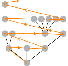
Figure 1: Illustration of the breadth-first exploration of vertices in a finite rooted tree. The vertices are explored according to the direction of the orange arrows.

In this section, random forests will conveniently span the components of a coupled multiplicative coalescent. In Section 2.1 these processes will be explored similarly to [Lim19], with a new feature: the non-spanning or surplus or excess edges will be recorded in addition. After that, in Section 3 another graph representation will be proposed in order to preserve the monotonicity of the graph-valued process.

2.1 Breadth-first order induced forest and surplus

Recall the definition of $Z^{\boldsymbol{x},q}$ in (2). As recalled in the introduction, an important observation from [Lim19] is that, simultaneously for all $q$, the component masses of the multiplicative coalescent started from $\boldsymbol{x}$ and evaluated at time $q$ can be coupled to $Z^{\boldsymbol{x},q}$ via a breadth-first walk construction. We next recall the above-mentioned construction. See Section 2 in [Lim19] for more details.

Given $a<b$ and an interval $[c,d]$ where $0\leq c<d$, define $(a,b]\oplus[c,d]:=(a+c,b+d],$ and denote by $|I|$ the Lebesgue measure of a Borel set $I$. Typically $I$ will be an interval. Let us also define $\xi^{q}_{(i)}:=\xi_{(i)}/q$.

Algorithm 1 constructs the vector of component sizes associated to the simultaneous breadth-first walk defined by (2). Algorithm 1 takes as arguments the vector $\boldsymbol{x}$ and the exponential random vector $\boldsymbol{\xi}$, and constructs, for a given $q>0$, the edges $V$ of the random forest coupled to the simultaneous breadth-first walk, denoted by $\mathcal{F}_{0}(q)$. In addition, the vector $\boldsymbol{Y}(q)$ contains the sizes of all the trees (connected components) that were discovered up to the current step.

$F_{0}^{q}\leftarrow\{0\}$

  // initializing the load-free periods

1

$I_{0}^{q}\leftarrow\{0\}$

  // initializing the listening periods

2

$i\leftarrow 1$

  // counter of the number of nodes

3

$k\leftarrow 0$

  // counter of the number of trees (connected components)

4

$\boldsymbol{Y}(q)\leftarrow\mathbf{0}$

  // (unordered) vector of component sizes at time $q$

5

6while $i\leqslant\operatorname{len}(\boldsymbol{x})$:

7      

      $j\leftarrow i$

        // auxiliary counter

8      

9      $k\leftarrow k+1$

      $F_{k}^{q}\leftarrow\Big{(}\sup\big{(}I_{i-1}^{q}\big{)},\xi_{(i)}/q\Big{]}$

        // $k^{\text{th}}$ load-free period

10      

      $I_{i}^{q}\leftarrow(\xi_{(i)}/q,\;\xi_{(i)}/q+x_{\pi_{i}}]$

        // $i^{\text{th}}$ listen period

11      

      $Y_{k}(q)\leftarrow Y_{k}(q)+x_{\pi_{i}}$

        // updating the component sizes

12      

13      while $i\leq j\leq\mathrm{len}(\boldsymbol{x})$:

14            

15            for each $\xi_{(r)}/q\in I_{i}^{q}\setminus I_{i-1}^{q}$ :

                   add edge $(\pi_{r}\to\pi_{i})$ to $V$

                    // $\pi_{r}$ is a children of $\pi_{i}$

16                  

                  $Y_{k}(q)\leftarrow Y_{k}(q)+x_{\pi_{r}}$

                    // updating component sizes

17                  

18                  $j\leftarrow j+1$

19            

20            

            $I_{i+1}^{q}\leftarrow I_{i}^{q}\oplus[0,x_{\pi_{i+1}}]$

              // updating the listen period

21            

22            $i\leftarrow i+1$

23      

24      

25

26

27return $V$ and $\boldsymbol{Y}(q)$

Algorithm 1 Implementation of the breadth-first walk algorithm, for given $\boldsymbol{\xi}$ and $\boldsymbol{x}$. At each time $q\geq 0$ this constructs a random forest on $\{1,2,\dots,\operatorname{len}(\boldsymbol{x})\}$ with vertices $V$ and whose vector of component sizes $\boldsymbol{Y}(q)$, ordered, evolves according to the multiplicative coalescent dynamic as $q$ varies.

Let us now explain this construction in words. For $k=1$ or $k$ equal to some of the values assigned when the Algorithm 1 visits line 1, the corresponding $\pi_{k}$ is the root of a new tree in $\mathcal{F}_{0}(q)$. Notice that for such values we have $I^{q}_{k}\cap I^{q}_{k-1}=\emptyset$. The intervals $F^{q}_{k}$, for $k\geq 1$, are called load-free periods. For any other $l\leq\operatorname{len}(\boldsymbol{x})$, the corresponding vertex $\pi_{l}$ is not a root. In any case, for each $l\geq 1$, the dynamics “listens” for the children of $\pi_{l}$ during the interval $I^{q}_{l}\setminus I^{q}_{l-1}$, and these are called the listening periods. This is implemented using the for cycle in line 1 of Algorithm 1. Furthermore, for each $h$ such that $\xi^{q}_{(h)}\in I^{q}_{l}\setminus I^{q}_{l-1}$, we have that $\pi_{l}$ (resp. $\pi_{h}$) is the parent (resp. child) of $\pi_{h}$ (resp. $\pi_{l}$) in $\mathcal{F}_{0}(q)$. In symbols, we write $\pi_{h}\to\pi_{l}$, thinking that any directed edge points to the parent, i.e. towards the root.

Finally, the above construction produces for each $q>0$ a random forest $\mathcal{F}_{0}(q)$ with vertex set $[\operatorname{len}(\boldsymbol{x})]$ and edge set $V$. The output value of $k$ is the number of trees in the forest $\mathcal{F}_{0}(q)$ and the vector

$$\boldsymbol{X}^{\boldsymbol{x}}(q):=\operatorname{ord}\big{(}(Y_{1}(q),Y_{2}(q),\dots,Y_{k}\textbf{}(q),0,\dots)\big{)}$$ (4)

where the vector $\boldsymbol{Y}(q)=(Y_{1}(q),Y_{2}(q),\dots,Y_{k}(q),0,\dots)$ is the output of Algorithm 1, records the masses of the components of $\mathcal{F}_{0}(q)$, i.e. the masses of the trees according to the weights (or equivalently, the masses of original particles given at time $0$) in $\boldsymbol{x}$. We naturally extend this definition at $q=0$ to a trivial forest of $\operatorname{len}(\boldsymbol{x})$ many single vertex trees ordered according to the order induced by $\boldsymbol{\xi}$.

Note that Algorithm 1 simultaneously constructs the vector $\boldsymbol{Y}(q)$ of components sizes at time $q$, as well as the random forest $\mathcal{F}_{0}(q)$. In order to achieve this, we introduced an auxiliary counter $j$ in line 1. This counter is used in the while cycle, starting at line 1, for counting the number of “listening periods” that need to be analyzed during the construction of each tree in $\mathcal{F}_{0}$. Algorithm 1 is not intended to be optimal. It is a choice, out of a number of possible pseudo-codes for the breadth-first walk algorithm. We believe that it could improve the readers’ understanding of the above construction. Again, we refer the interested reader to Section 2 in [Lim19] for more details on the construction of the random forest $\mathcal{F}_{0}(q)$ associated to the simultaneous breadth-first walk $Z^{\boldsymbol{x},q}$.

Define

$$B^{\boldsymbol{x},q}(s):=Z^{\boldsymbol{x},q}(s)-\inf_{u\leq s}Z^{\boldsymbol{x},q}(u),\ s\geq 0,\ q>0.$$

Due to the above made observations, if (and only if) at time $s$ a new vertex is seen (or “heard”) in $\mathcal{F}_{0}(q)$, the process $Z^{\boldsymbol{x},q}$ (and therefore $B^{\boldsymbol{x},q}$) makes a jump up by the amount equal to the mass of that vertex. Let $k$ take a value assigned by the Algorithm 1 during a passage through line 1. The total sum of upward jumps of $B^{\boldsymbol{x},q}$ during $T_{k}(q):=\operatorname{Cl}(I_{k}^{q})$ is entirely compensated by the unit downward drift of $Z^{\boldsymbol{x},q}$ (or $B^{\boldsymbol{x},q}$) during $T_{k}(q)$. It is also easy to see that $B^{\boldsymbol{x},q}(s)>0$ in the interior of $T_{k}(q)$. Therefore, the $k^{\text{th}}$ excursion of $(B^{\boldsymbol{x},q},\ q>0)$ above $0$ has the length precisely equal to the sum of the masses of all the blocks (vertices of the tree) explored during $T_{k}(q)$, i.e. $|T_{k}(q)|=Y_{k}(q)$. It was initially noted in [Lim19], whose approach is rooted in [Ald97, AL98], that for each fixed $q$, the ordered excursion lengths $\boldsymbol{X}^{\boldsymbol{x}}(q)$, as defined by (4), have the multiplicative coalescent distribution, started from $\boldsymbol{x}$ and evaluated at time $q$. In particular, the exiting $k(q)\leq\operatorname{len}(\boldsymbol{x})$ in the above algorithm, clearly equals to the number of connected components at time $q$ of the coupled Aldous’ continuous-time random graph. This type of result can be called static, since it characterizes the marginal law of the process.

The advantage of the simultaneous breadth-first walk is that it also allows us to obtain a dynamical result, characterizing the trajectories of the MC. Proposition 5 in [Lim19] shows the following stronger claim: $(\boldsymbol{X}^{\boldsymbol{x}}(q),q\geq 0)$ has the multiplicative coalescent law as a process in $q$, where the initial state at time $0$ is $\boldsymbol{x}$.

One might wish to strengthen this in saying that the above coupling of $Z^{\boldsymbol{x},q}$ and $\mathcal{F}_{0}(q)$ provides a bijective matching between the $k^{\text{th}}$ excursion of $B^{\boldsymbol{x},q}$ above $0$, necessarily started at $\xi_{(h)}^{q}$ for some $h\in[\operatorname{len}(\boldsymbol{x})]$, and a spanning (breadth-first explored) tree rooted at $\pi_{h}$ of the unique component of the continuous-time random graph which contains $\pi_{h}$ at time $q$. Some care is however needed here. Indeed, while the mergers of different connected components or different subtrees of $\mathcal{F}_{0}(\cdot)$ arrive at precisely the multiplicative rate, the new edges arriving in $\mathcal{F}_{0}$ that correspond to those mergers always connect the root of one of the components (its excursion starts at $\xi_{(h)}^{q}$ in $B^{\boldsymbol{x},\cdot\,-}$) to the last visited or listed vertex in the previous component (its excursion is the one starting just before $\xi_{(h)}^{q}$ in $B^{\boldsymbol{x},\cdot\,-}$). In addition, within each connected component the edges evolve according to a peculiar “prune and reconnect” rule, where vertices and subtrees are gradually “moved closer” to the root. Note that $\mathcal{F}_{0}(0)$ is the forest consisting in $\operatorname{len}(\boldsymbol{x})$ isolated vertices, and for $q$ large enough, $\mathcal{F}_{0}(q)$ is the tree rooted at $\pi_{1}$ with $\operatorname{len}(\boldsymbol{x})-1$ descendants. In particular, the forest $(\mathcal{F}_{0}(q),\,q\geq 0)$ is not a monotone process with respect to the order induced by the subgraph relation. Still, $\mathcal{F}_{0}(\cdot)$ is a random forest-valued process, whose tree masses evolve precisely according to (1), so it is a MC graph representation. We refer to any edge of $\mathcal{F}_{0}(q)$ as an spanning edge at time $q$.

2.2 Surplus on top of $\mathcal{F}_{0}$

There is a natural way to build the surplus or excess edges on top of $\mathcal{F}_{0}(q)$, for each $q$ separately, so that the distribution of the resulting graph is exactly the marginal of the continuous-time random graph at time $q$. Since there are no loops or multi-edges in the continuous-time random graph $\big{(}\mathcal{G}^{\boldsymbol{x}}(q),q\geq 0\big{)}$, we only need to check if there is a surplus edge between each pair of vertices which are connected, but not by an edge in $\mathcal{F}_{0}(q)$.

Let us assume, without loss of generality, that we are looking for the surplus edges in the first tree in the random forest $\mathcal{F}_{0}(q)$. Indeed, because of the lack of memory property of the exponential distribution, after exploring one or several components, the residual exponential times of the unexplored vertices have the same distribution as a family of “new” exponentials, independent from the past. Suppose that for some $h\in[2,\operatorname{len}(\boldsymbol{x})]$ we have that $\pi_{h}$ belongs to the first tree, that is $\xi_{(h)}^{q}\in I_{h-1}^{q}:=(\pi_{(1)}^{q},\pi_{(1)}^{q}+x_{\pi_{1}}+\dots+x_{\pi_{h-1}}]$. Take $j\in[2,\operatorname{len}(\boldsymbol{x})]$, also in the first tree, such that $\xi_{j}\geq\xi_{(h)}$, i.e. $j$ comes after $\pi_{h}$ according to the breadth first order. Then, if

$$\xi_{j}^{q}\in\big{(}\xi_{(1)}^{q}+x_{\pi_{1}}+\dots+x_{\pi_{h-1}},\xi_{(1)}^{q}+x_{\pi_{1}}+\dots+x_{\pi_{h-1}}+x_{\pi_{h}}\big{]}$$

the edge $j\to\pi_{h}$ belongs to $\mathcal{F}_{0}(q)$, and this happens with probability $1-\mathrm{e}^{-q\,x_{\pi_{h}}\,x_{j}}$. This is a consequence of the breadth-first procedure (see [Lim19, § 2]) and of the lack of memory of the exponential distribution. Indeed, let us denote

$$\mathcal{Z}^{q}_{s}=\sigma\left(\{(\xi_{i}^{q}>u):i\in[\operatorname{len}(\boldsymbol{x})]\},u\leq s\right).$$

Hence, $(\mathcal{Z}_{s}^{q})_{s\geq 0}$ is the filtration generated by the arrivals of $(\xi_{1}^{q},\xi_{2}^{q},\dots)$ and recall that

$$\{\xi_{j}^{q}>\sup(I_{h-1}^{q})\}=\{\xi_{j}^{q}>\xi_{(1)}^{q}+x_{\pi_{1}}+\dots+x_{\pi_{h-1}}\}\in\mathcal{Z}_{\sup(I_{h-1}^{q})}^{q}.$$

Then, we have

$$\mathbb{P}\left(\xi_{j}^{q}>\sup(I_{h}^{q})\mid\mathcal{Z}_{\sup(I_{h-1}^{q})}^{q}\right)\mathbb{1}_{(\xi_{j}>\xi_{(h)})}=\mathrm{e}^{-q\,x_{j}\,x_{\pi_{h}}}\mathbb{1}_{(\xi_{j}>\xi_{(h)})}\;\;\text{ a.s.}$$

Note that $\mathrm{e}^{-q\,x_{j}\,x_{\pi_{h}}}$ is precisely the probability that vertices $j$ and $\pi_{h}$ are not connected at time $q$ in the Aldous’ continuous-time random graph dynamic. Hence, the breadth-first walk does not only construct the spanning edges according to the random graph dynamics, but also ensures the nonexistence of the edges $j\to\pi_{h}$, where $j$ is any vertex listed after the children of $h$ in the breadth-first order induced by the algorithm. Note that, if $\xi_{j}^{q}\in(\xi_{(h)}^{q},\sup(I_{h-1}^{q})]$, then $j$ is necessarily another vertex in the same tree, attached to it after $\pi_{h}$ and before any child of $\pi_{h}$. Thus, due to the breadth-first exploration order, see Figure 1, there are only two possibilities:

1. $j$ is listed after $\pi_{h}$, in the same generation as $\pi_{h}$, or

2. $j$ is from the next generation (then necessarily a child of some vertex $\pi_{k}$ with $k<h$, where $\pi_{k}$ is from the same generation as $\pi_{h}$).

See Figures 2(a) and 2(b) for an illustration of these two cases.

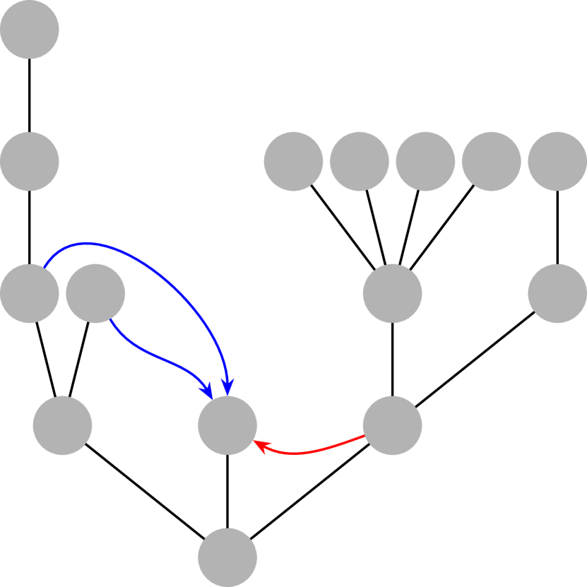
(a)

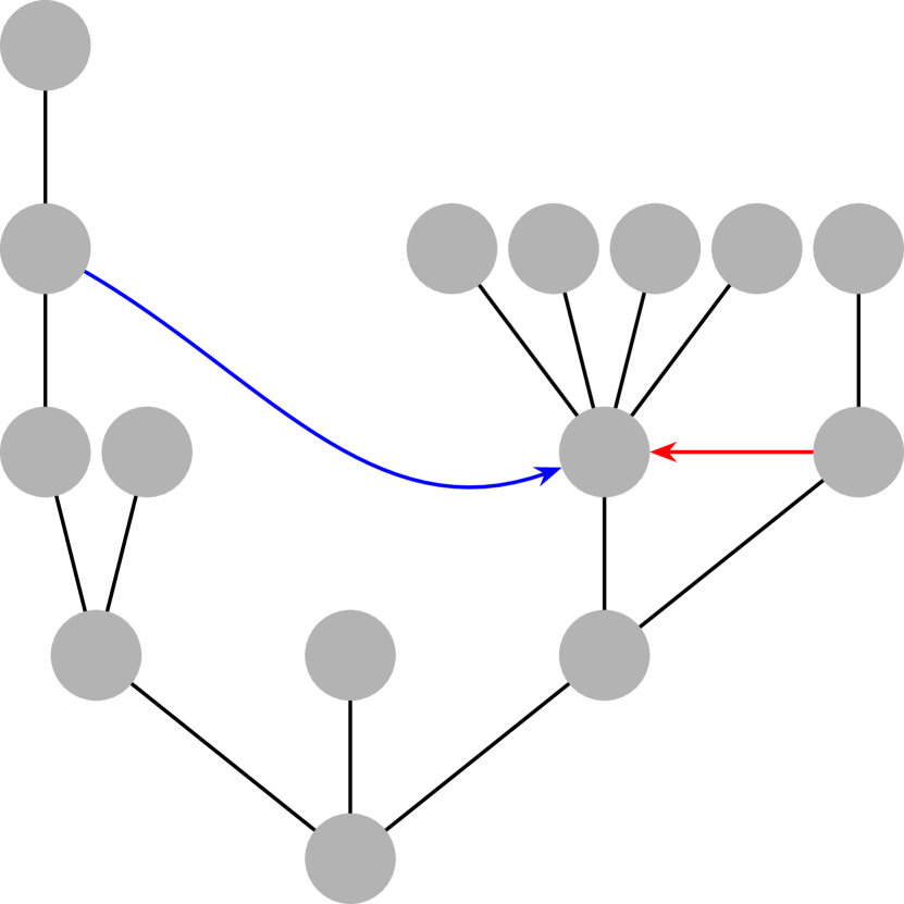
(b)

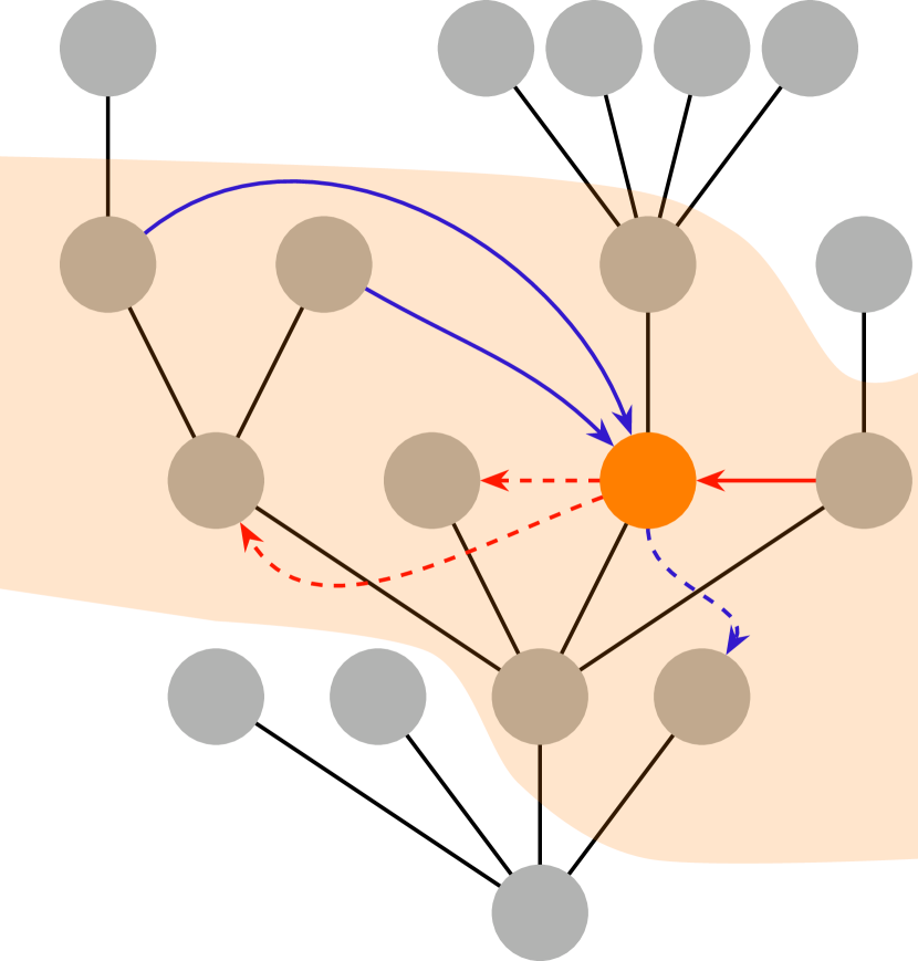
(c)

Figure 2: Figures 2(a) and 2(b) show two different configurations and the surplus edges going to the third and the seventh vertices in the breadth-first order, respectively. Possible surplus edges coming from vertices in the same generation as described in (i) are indicated in red, and those from vertices in the next generation as described in (ii) are indicated in blue. Figure 2(c) shows the influence region of the orange vertex, the eighth vertex in the breadth-first order. The red/blue coloring meaning is the same as in Figures 2(a) and 2(b). The arrows indicating a possible surplus edge between the orange vertex and a previously (resp. subsequently) listed vertex are dashed (resp. solid).

The oriented surplus edges with arrows pointing to $j$ are possible only from those indices $j$ satisfying (a) or (b). Indeed, if $j$ is listed after all the children of $\pi_{(h)}$ then there is no spanning or surplus edge connecting $j$ and $\pi_{(h)}$. If $\xi_{j}^{q}$ enters $I_{h}^{q}\setminus I_{h-1}^{q}$, as noted above, this means that $j$ is a child of $\pi_{h}$ (which prohibits existence of a surplus edge connecting them). Finally, if $\xi_{j}^{q}\in I_{h-1}^{q}\setminus[0,\xi_{(h)}^{q}]=(\xi_{(h)}^{q},\sup(I_{h-1}^{q})]$ then either (a) or (b) are true, and a surplus edge connecting $j$ and $\xi_{(h)}$ is not excluded by the algorithm. So, one needs an external source of randomness to determine whether the surplus edge exists or not.

Figure 2(c) below shows the “surplus influence region” for a typical non-root vertex. Note that the surplus influence region of a given vertex $v$ consists of all the vertices attached to the tree (strictly) between the parent of $v$ and the first child of $v$, in the sense of the order induced by breadth-first algorithm.

The presence or absence of surplus edges is of course determined according to the random graph dynamic. For each $l,h\in[\operatorname{len}(\boldsymbol{x})]$, let $\zeta^{l,h}$ be a Poisson process of marks arriving at rate $x_{l}$, independently over $l$ and $h$. Consider those (and only those) $\zeta^{l,h}$ such that $\xi_{l}^{q}\in I_{h-1}^{q}$. For any such $l$ draw the (red or blue) surplus edge connecting $l$ and $\pi_{h}$ if and only if $\zeta^{h,l}[0,q\cdot x_{\pi_{h}}]\geq 1$. It is clear that this edge appears with probability $1-\mathrm{e}^{-q\,x_{l}\,x_{\pi_{h}}}$, independently of everything else. Any other edge at time $q$ is also present with probability $1-\mathrm{e}^{-q\,m_{1}\,m_{2}}$, where $m_{1}$ and $m_{2}$ are the masses of the two vertices (see above discussion and Section 2 in [Lim19] for more details).

Denote by $G^{\boldsymbol{x}}(q)=(V,E(q))$ the resulting random graph, where $E(q)$ is the union of the spanning and the surplus edges at time $q$. One can record the just made observations as follows.

Lemma 2.1.

For each $q\geq 0$ and every finite vector $\boldsymbol{x}$, the random graph $G^{\boldsymbol{x}}(q)$ has the law of the Aldous’ continuous-time random graph evaluated at time $q$, i.e. it has the same distribution as $\mathcal{G}^{\boldsymbol{x}}(q)$.

Remark 2.1 (Joint intensity of the Poisson processes).

Suppose that one is only interested in counting the surplus edges in various connected components of the random graph, without keeping track of their exact location (the vertices which it connects). Then, note that the joint (total) intensity of all the Poisson marking processes $\zeta^{l,h}$ for a fixed value of $h$ is

$$q\cdot\sum_{l>h,\,\xi_{(l)}^{q}\in I_{h-1}^{q}}x_{\pi_{l}} =q\left(\sum_{s\in I_{h-1}^{q}}\Delta Z^{\boldsymbol{x},q}(s)-|I_{h}^{q}|\right)=q\Big{(}B^{\boldsymbol{x},q}\big{(}\sup(I_{h-1}^{q})\big{)}-x_{\pi_{h}}\Big{)},$$ (5)

where $\Delta Z^{\boldsymbol{x},q}(s):=Z^{\boldsymbol{x},q}(s)-Z^{\boldsymbol{x},q}(s-)$, and we recall that $B^{\boldsymbol{x},q}$ equals $Z^{\boldsymbol{x},q}$ reflected above past minima. Indeed, the first identity in (5) is a consequence of the following identities

$$\sum_{l:\xi_{(l)}\in I_{h-1}^{q}}x_{\pi_{l}}=\sum_{s\in I_{h-1}^{q}}\Delta Z^{\boldsymbol{x},q}(s)\;\;\text{ and }\;\;|I_{h}^{q}|=x_{\pi_{k}}+\dots+x_{\pi_{h}},$$

where $\pi_{k}$ is the root of the tree including $\pi_{h}$ as one of its vertices. To check the second identity in (5) note that, due to the drift in the definition of $Z^{\boldsymbol{x},q}$, as well as the definition of the reflection map transforming $Z^{\boldsymbol{x},q}$ into $B^{\boldsymbol{x},q}$, we have

$$B^{\boldsymbol{x},q}\Big{(}\sup(I_{h-1}^{q})\Big{)}=\sum_{s\in I_{h-1}^{q}}\Delta Z^{\boldsymbol{x},q}(s)-|I_{h-1}^{q}|.$$

Recall that $Z^{\boldsymbol{x},q}$ does not typically attain its global infimum on $[0,\sup(I_{h}^{q})]$. However, its infimum on the interval $[0,\sup(I_{h}^{q})]$ is always equal to the left limit $Z^{\boldsymbol{x},q}(\xi_{(k)}^{q}-)$ of $Z^{\boldsymbol{x},q}$ evaluated at the left endpoint $\inf(I_{h}^{q})=\xi_{(k)}^{q}$ of $I_{h}^{q}$. Here $\pi_{k}$ is the root of the corresponding tree (as in the previous paragraphs).

The next remark is a digression which could help an interested reader in understanding the relation between (5) and the rate of surplus edge arrival in the near-critical regime. Our second construction of surplus edges (in Section 3) leads to a precise formulation and analysis of an analogous property. In Section 4 we discuss some interesting consequences of this for the near-critical regime.

Remark 2.2 (The link between the surplus edges and the area below the curve).

The total rate of the Poisson process generating the surplus edges issued from $\pi_{h}$, as constructed in Section 2.2, can be computed using (5) and we get

$$A_{h}=q\cdot x_{\pi_{h}}\cdot\sum_{l>h,\,\xi_{(l)}^{q}\in I_{h-1}^{q}}x_{\pi_{l}}=q\Big{(}x_{\pi_{h}}\cdot B^{\boldsymbol{x},q}\big{(}\sup(I_{h-1}^{q})\big{)}-x_{\pi_{h}}^{2}\Big{)}.$$

Hence, the total number of unlimited surplus edges within the connected component $C_{i}$ is a Poisson random variable with mean

$$\sum_{h:\,\pi_{h}\in C_{i}}A_{h}=\sum_{h:\,\pi_{h}\in C_{i}}q\Big{(}x_{\pi_{h}}\cdot B^{\boldsymbol{x},q}\big{(}\sup(I_{h-1}^{q})\big{)}-\big{(}x_{\pi_{h}}\big{)}^{2}\Big{)}.$$

In the scaling limit (see [Lim19, Prop. 1.6] or Section 4 below) we get

$$\lim\limits_{n\to\infty}q_{n}(t)\sum_{h:\,\pi_{h}\in C_{i}^{(n)}}\Big{(}x_{\pi_{h}}^{(n)}\cdot B^{\boldsymbol{x}^{(n)},q_{n}(t)}\big{(}\sup(I_{h-1}^{q})\big{)}-\big{(}x_{\pi_{h}}^{(n)}\big{)}^{2}\Big{)}=\int_{a_{i-1}}^{a_{i}}B^{\kappa,t,\boldsymbol{c}}(s)\mathrm{d}s,$$

where $a_{i-1}$ and $a_{i}$ are the left endpoint and the right endpoint of the $i^{\text{th}}$ largest excursion of $B^{\kappa,t,\boldsymbol{c}}$ (defined in (11)) above zero, $\boldsymbol{x}^{(n)}$ satisfies conditions (5.1)-(5.3) in [Lim19] (which are (12), (13), (14) below) and $q_{n}(t)=t+1/\sigma_{2}^{(n)}$, where $\sigma_{2}^{(n)}=\sum(x_{i}^{(n)})^{2}$. Indeed,

$$\sum_{h:\,\pi_{h}\in C_{i}^{(n)}}x_{\pi_{h}}^{(n)}\cdot q_{n}(t)B^{\boldsymbol{x}^{(n)},q_{n}(t)}\big{(}\sup(I_{h-1}^{q})\big{)}$$

is a Riemann sum of $q_{n}(t)B^{\boldsymbol{x}^{(n)},q_{n}(t)}$ for $s\in[a_{i}^{(n)},b_{i}^{(n)}]$, the excursion interval of $B^{\boldsymbol{x}^{(n)},q_{n}(t)}$ above zero, and in the scaling limit this function converges towards $B^{\kappa,t,\boldsymbol{c}}$ in the sense of the $J_{1}$ topology [Lim19, Prop. 6]. In addition, the error term

$$q_{n}(t)\sum_{h:\,\pi_{h}\in C_{i}^{(n)}}(x_{\pi_{h}}^{(n)})^{2}=\left(t+\frac{1}{\sigma_{2}^{(n)}}\right)\sum_{h:\,\pi_{h}\in C_{i}^{(n)}}(x_{\pi_{h}}^{(n)})^{2}$$

can be controlled by using (5.1)-(5.3) in [Lim19] (which are (12), (13), (14) below).

Furthermore, the number of surplus edges in the limited regime is a sum of independent Bernoulli random variables with parameters converging to zero and such that the sum of the parameters converges to $\int_{a_{i-1}}^{a_{i}}B^{\kappa,t,\boldsymbol{c}}(s)\mathrm{d}s$. Hence, using Le Cam’s inequality [LC60, Thm. 2], i.e. the classic approximation of the sum of independent Bernoulli random variables by a Poisson distribution, we get that the number of limited surplus edges is also $Y_{i}$. This idea was used by the authors in a companion paper [CL23, Cor. 1.2 ] to exhibit the scaling limit of the critical Erdős – Rényi (limited) random graph.

3 Monotone forest representation and surplus edges

We next revise and enrich (via an additional randomization) the coupling algorithm just described. Instead of the random forest process $(\mathcal{F}_{0}(q),\,q>0)$, another forest-valued process $(\mathcal{F}_{1}(q),\,q>0)$ is described, so that it is motonone ($\mathcal{F}_{1}(q_{1})$ is a subgraph of $\mathcal{F}_{1}(q_{2})$ when $q_{1}\leq q_{2}$). The process $\mathcal{F}_{1}$ is linked to the dynamic of the Aldous’ random graph in a sense that we now explain.

As before, let us fix a finite vector $\boldsymbol{x}$. Let $\big{(}\mathcal{G}^{\boldsymbol{x}}(q),q\geq 0\big{)}$ be the inhomogeneous random graph started from $\operatorname{len}(\boldsymbol{x})$ many isolated nodes of masses $\boldsymbol{x}$. Let $\big{(}\boldsymbol{X}^{\boldsymbol{x}}(q),q\geq 0\big{)}$ be the MC coupled to $\big{(}\mathcal{G}^{\boldsymbol{x}}(q),q\geq 0\big{)}$, i.e. the process where $\boldsymbol{X}^{\boldsymbol{x}}(q)$ records the size of the connected components in $\mathcal{G}^{\boldsymbol{x}}(q)$, for every $q\geq 0$. Consider now a forest-valued process $\big{(}\mathcal{T}^{\boldsymbol{x}}(q),q\geq 0\big{)}$ such that, $\big{(}\mathcal{T}^{\boldsymbol{x}}(q),q\geq 0\big{)}$ only jumps when $\big{(}\boldsymbol{X}^{\boldsymbol{x}}(q),q\geq 0\big{)}$ does, i.e. when two connected components of $\mathcal{G}^{\boldsymbol{x}}(q-)$ merge into one new component of $\mathcal{G}^{\boldsymbol{x}}(q)$. A jump of $\big{(}\mathcal{T}^{\boldsymbol{x}}(q),q\geq 0\big{)}$ consists in adding an edge to the graph, and the new edge in $\mathcal{T}^{\boldsymbol{x}}(q)$ is precisely the new edge appearing in $\big{(}\mathcal{G}^{\boldsymbol{x}}(q),q\geq 0\big{)}$ at the moment of the jump, i.e. it is the edge which produces the merger. One can deduce from the previous construction that $\big{(}\mathcal{T}^{\boldsymbol{x}}(q),q\geq 0\big{)}$ satisfies the following properties:

1. $\big{(}\mathcal{T}^{\boldsymbol{x}}(q),q\geq 0\big{)}$ is a forest-valued Markov process,

2. $\big{(}\mathcal{T}^{\boldsymbol{x}}(q),q\geq 0\big{)}$ is monotone in the sense of the inclusion of sets,

3. for every $q\geq 0$, $\mathcal{T}^{\boldsymbol{x}}(q)$ is a spanning forest of $\mathcal{G}^{\boldsymbol{x}}(q)$, meaning each tree in $\mathcal{T}^{\boldsymbol{x}}(q)$ is a spanning tree of some connected component of $\mathcal{G}^{\boldsymbol{x}}(q)$.

4. given the past and present configurations $\sigma(\mathcal{T}^{\boldsymbol{x}}(z):z\leq q)$, and knowing that the random graph at time $q$ (resp. the random forest $\mathcal{T}^{\boldsymbol{x}}(q)$) has $N$ connected components (resp. spanning trees), which induce a partition

   $$\{i_{1},i_{2},\ldots,i_{k_{1}}\},\{i_{k_{1}+1},i_{k_{1}+2},\ldots,i_{k_{2}}\},\dots,\{i_{k_{N-1}+1},i_{k_{N-1}+2},\ldots,i_{\operatorname{len}(\boldsymbol{x})}\}$$

   on $[\operatorname{len}(\boldsymbol{x})]$ (without knowing the breadth-first order induced by $\boldsymbol{\xi}$, but knowing that the mass of $i$ equals $x_{i}$), the edge between any two $h$ and $l$, which belong to different trees of $\mathcal{T}^{\boldsymbol{x}}(q)$, arrives at rate $x_{h}\cdot x_{l}$.

Several random forests can be constructed such that properties M.1, M.2 and M.3 are satisfied. For example, we can construct a trivial such random forest in the following way: for each $h\in[2,\operatorname{len}(\boldsymbol{x})]$, $\pi_{h}$ always gets connected by an edge to $\pi_{h-1}$ at the moment when its connected component merges with another (previously listed) connected component ($\pi_{h}$ served as the root of its component just prior to the merger time). This unsophisticated procedure constructs a monotone forest-valued process that evolves starting from the forest of $\operatorname{len}(\boldsymbol{x})$ many trivial trees (i.e. $\mathcal{F}_{0}(0)$), and ending with a tree of $\operatorname{len}(\boldsymbol{x})$ many generations, with a single vertex in each generation. However, the edge arrivals in this construction do not satisfy M.4. Indeed, if two connected components, composed of $\{i_{1},i_{2},i_{3}\}$ and $\{i_{4},i_{5}\}$, merge at a certain time $q$ via an edge connecting $i_{2}$ and $i_{5}$, then (given all the available information) we know that starting from time $q$ both $i_{2}$ and $i_{5}$ are interior vertices within the tree containing $\{i_{1},i_{2},i_{3},i_{4},i_{5}\}$, and therefore it is not possible for either of these vertices to connect via an edge to any other vertex at a future merging event.

The process $\big{(}\mathcal{T}^{\boldsymbol{x}}(q),q\geq 0\big{)}$ can be thought of as a dynamical spanning forest coupled to the random graph $\big{(}\mathcal{G}^{\boldsymbol{x}}(q),q\geq 0\big{)}$. Our goal in this section is to construct a forest valued process $\big{(}\mathcal{F}_{1}(q),q\geq 0\big{)}$ coupled to the simultaneous breadth-first walk $(Z^{{\boldsymbol{x}},q},q\geq 0)$, such that it has the same distribution as $\big{(}\mathcal{T}^{\boldsymbol{x}}(q),q\geq 0\big{)}$.

Let us take a deeper look into the dynamic of the process $\big{(}\mathcal{T}^{\boldsymbol{x}}(q),q\geq 0\big{)}$. This Markov process jumps according to the multiplicative coalescent rates $X_{i}\cdot X_{j}$, where $X_{i}$ and $X_{j}$ are the total masses of two connected components (trees) in $\mathcal{T}^{\boldsymbol{x}}(q)$. Conditionally on the fact that the components which are merging are $C_{i}=\{i_{1},\dots,i_{k}\}$ and $C_{j}=\{j_{1},\dots,j_{m}\}$, such that $|C_{i}|=X_{i}=x_{i_{1}}+\dots+x_{i_{k}}$ and $|C_{j}|=X_{j}=x_{j_{1}}+\dots+x_{j_{m}}$, and that the coalescence time is $Q$, the new edge in $\mathcal{T}^{\boldsymbol{x}}(Q)$ is $\{i_{s},j_{t}\}$ with probability

$$\frac{x_{i_{s}}}{X_{j}}\frac{x_{j_{t}}}{X_{j}},\text{ for every }i_{s}\in C_{i}\text{ and }j_{t}\in C_{j}.$$

Indeed, suppose that, for $i_{s}\in C_{i}$, $j_{t}\in C_{j}$, $\zeta^{i_{s},j_{t}}$ is an exponential random variable with rate $x_{i_{s}}\cdot x_{j_{t}}$, independently over different $s$ and $t$. Then, according to the random graph dynamic and elementary properties of the exponential distribution, on the event $\{Q=q\}$ the edge $\pi_{i_{s}}\to\pi_{j_{t}}$ is the one created by the merger of $C_{i}$ and $C_{j}$ with probability

$$\mathbb{P}\left[\zeta^{i_{s},j_{t}}=\min_{k\in C_{i},l\in C_{j}}\zeta^{k,l}\,\Big{|}\,\min_{k\in C_{i},l\in C_{j}}\zeta^{k,l},\mathcal{T}^{\boldsymbol{x}}(q-)\right] \equiv\frac{q\cdot x_{i_{s}}x_{j_{t}}}{\sum\limits_{k\in C_{i},l\in C_{j}}q\cdot x_{k}x_{l}}=\frac{x_{i_{s}}}{X_{i}}\frac{x_{j_{t}}}{X_{j}}.$$

This is equivalent to picking one vertex in each component according to the size biased order, and creating the edge between them. The arrival of this edge reduces the total number of trees by one (it creates one tree from two smaller trees).

We now describe the construction of $(\mathcal{F}_{1}(q),q\geq 0)$. The initial forest $\mathcal{F}_{1}(0)$ is again trivial, and therefore equal to $\mathcal{F}_{0}(0)$. It is the set of vertices $[\operatorname{len}(\boldsymbol{x})]$, without any edge. During a strictly positive (random) interval of time $\mathcal{F}_{1}(\cdot)$ will remain $\mathcal{F}_{1}(0)$. At some (stopping) time $Q_{1}>0$ the first connection is established between $\pi_{L}$ and $\pi_{L-1}$, where $L$ is the first value in $[\operatorname{len}(\boldsymbol{x})]$ such that $\xi_{(L)}^{Q_{1}}\in I_{L-1}^{Q_{1}}=(\xi^{Q_{1}}_{(L-1)},\xi^{Q_{1}}_{(L-1)}+x_{\pi_{L-1}}]$. In particular, $\xi_{(h)}^{Q_{1}}\not\in I_{h-1}^{Q_{1}}$ for any $h\in[2,\operatorname{len}(\boldsymbol{x})]\setminus\{L\}$. At time $Q_{1}$ both $\mathcal{F}_{0}$ and $\mathcal{F}_{1}$ make the same jump: the new edge $\pi_{L}\rightarrow\pi_{L-1}$ appears. After that, during an interval of time of positive random length, $\mathcal{F}_{1}$ stays equal to $\mathcal{F}_{1}(Q_{1})$, and eventually a new connection occurs at some time $Q_{2}>Q_{1}$. The difference between $\mathcal{F}_{1}$ and $\mathcal{F}_{0}$ may be visible already at time $Q_{2}$. Indeed, for the sake of illustration suppose that either $\xi_{(L+1)}^{Q_{2}}$ enters $I_{L}^{Q_{2}}=(\xi^{Q_{2}}_{(L-1)},\xi^{Q_{2}}_{(L-1)}+x_{\pi_{L-1}}+x_{\pi_{L}}]$, or $\xi_{(L-1)}^{Q_{2}}$ enters $I_{L-2}^{Q_{2}}=(\xi^{Q_{2}}_{(L-2)},\xi^{Q_{2}}_{(L-2)}+x_{\pi_{L-2}}]$ at this very moment. As already noted, in $\mathcal{F}_{0}(Q_{2})$ we will add the edge $\pi_{L+1}\rightarrow\pi_{L}$ in the first case, and $\pi_{L-1}\rightarrow\pi_{L-2}$ in the second case. Also note that in $\mathcal{F}_{0}$ both $\pi_{L}$ and $\pi_{L-1}$ will eventually become children of the same vertex $\pi_{h}$ for some $h\in\{1,\dots,L-1\}$ and this $h$ will change until finally becoming equal to $\pi_{1}$. However, in the first case, the new edge in $\mathcal{F}_{1}(Q_{2})$ is

• $\pi_{L+1}\rightarrow\pi_{L}$, with probability $\displaystyle\frac{x_{\pi_{L}}}{x_{\pi_{L-1}}+x_{\pi_{L}}}$, or

• $\pi_{L+1}\rightarrow\pi_{L-1}$, with the remaining probability $\displaystyle\frac{x_{\pi_{L-1}}}{x_{\pi_{L-1}}+x_{\pi_{L}}}$.

In the second case, the new edge in $\mathcal{F}_{1}(Q_{2})$ is either

• $\pi_{L-1}\rightarrow\pi_{L-2}$, with probability $\displaystyle\frac{x_{\pi_{L-1}}}{x_{\pi_{L-1}}+x_{\pi_{L}}}$, or

• $\pi_{L}\rightarrow\pi_{L-2}$, with the remaining probability $\displaystyle\frac{x_{\pi_{L}}}{x_{\pi_{L-1}}+x_{\pi_{L}}}$.

In $\mathcal{F}_{1}$, this and any other edge, once it appears, will remain in $\mathcal{F}_{1}$ forever after. It is important to note that these transitions are compatible with the evolution of $(\mathcal{T}^{\boldsymbol{x}}(q),q\geq 0)$.

The complete construction of $\mathcal{F}_{1}$ is as follows: $\mathcal{F}_{1}(0)=\mathcal{F}_{0}(0)$; for $q>0$, $\mathcal{F}_{1}(q)=\mathcal{F}_{1}(q-)$ unless $q$ is such that the number of components (trees) in $\mathcal{F}_{0}$ at time $q$ decreases by $1$. The latter happens if and only if for some $j\in[\operatorname{len}(\boldsymbol{x})]$, $\xi_{\pi_{j}}^{q-}\not\in I_{j-1}^{q-}$ ($\pi_{j}$ is a root in $\mathcal{F}_{0}(q-)$, or equivalently, in $\mathcal{F}_{1}(q-)$) and $\xi_{\pi_{j}}^{q}\in I_{j-1}^{q}$. Assume that the two components that merge at time $q$ in $\mathcal{F}_{0}(q)$ are $\{\pi_{i},\pi_{i+1},\dots,\pi_{j-1}\}\text{ and }\{\pi_{j},\pi_{j+1},\dots,\pi_{j+k}\}.$ For such $q$, let $\mathcal{F}_{1}(q)$ inherit all the edges of $\mathcal{F}_{1}(q-)$, and in addition

$$\text{draw a new edge }{L_{1}(q)}\rightarrow{L_{2}(q)}\mbox{ in }\mathcal{F}_{1}(q),$$ (6)

where $L_{1}(q)$ and $L_{2}(q)$ are chosen at random (in the size-biased way) from the vertices of the right-most and left-most components in $\mathcal{F}_{1}(q-)$ merging at $q$, i.e. from $\{\pi_{j},\pi_{j+1},\dots,\pi_{j+k}\}$ and $\{\pi_{i},\pi_{i+1},\dots,\pi_{j-1}\}$, respectively. More precisely, conditionally on $\{\mathcal{F}_{1}(s),\,s<q\}$ and $\{\mathcal{F}_{0}(s),\,s\leq q\}$, take $L_{1}(q)$ equal to $\pi_{s}$ with probability $x_{\pi_{s}}/(x_{\pi_{j}}+x_{\pi_{j+1}}+\dots+x_{\pi_{j+k}})$ for each $s\in\{j,j+1,\dots,j+k\}$, and $L_{2}(q)$ equal to $\pi_{l}$ with probability $x_{\pi_{l}}/(x_{\pi_{i}}+x_{\pi_{i+1}}+\dots+x_{\pi_{j-1}})$ for each $l\in\{i,i+1,\dots,j-1\}$, and finally apply (6).

It is clear from the just presented construction that $\mathcal{F}_{1}$ is a monotone forest-valued process, and also that, almost surely, for each $q$ the trees in $\mathcal{F}_{1}(q)$ are composed of exactly the same vertices as the (corresponding) trees in $\mathcal{F}_{0}(q)$ (or equivalently, $i$ and $j$ are connected in $\mathcal{F}_{1}(q)$ if and only if they are connected in $\mathcal{F}_{0}(q)$). Moreover, we obtain the following.

Lemma 3.1.

$(\mathcal{F}_{1}(q),q\geq 0)$ follows the same distribution as the dynamical spanning forest $(\mathcal{T}^{\boldsymbol{x}}(q),q\geq 0)$.

Remark 3.1.

The just described way of attaching edges in $\mathcal{F}_{1}$ is the most natural (if not the only) choice for a monotone MC forest representation coupled with the breadth-first walk. Indeed, to respect the order of vertices and connected components which is induced by the coupled walks $Z^{\boldsymbol{x},\cdot}$, one has no option but to attach one vertex from the two trees in $\mathcal{F}_{1}(q-)$ that are merging, and (6) means that the parent $L_{1}(q)$ and the child $L_{2}(q)$ are picked uniformly from the mass in those components (trees).

3.1 Surplus on top of $\mathcal{F}_{1}$

We refer to any edge of $\mathcal{F}_{1}(q)$ as spanning edge arriving before $q$. Note the difference with a similar and weaker definition in terms of $\mathcal{F}_{0}$. Our next goal is to account for the surplus edges in a way which is compatible with the coupled breadth-first walks $Z^{\boldsymbol{x},\cdot}$, and such that the monotonicity of the surplus edges is preserved in time.

Remark 3.2.

The construction of the surplus edges in Section 2.2 is not necessarily monotone in time, and it is simpler than the one we are about to describe. Recall that in the previous setting we only needed to check for the existence of the surplus edges in a certain neighborhood of each vertex, see Figure 2 for an illustration of this fact. However, this is no longer the case here, as our aim is to preserve the monotonicity. We need to use an external source of randomness evolving in time to check for all the surplus edges among all the available pairs of vertices within a connected component.

As the reader will see in Section 3.2, there is a natural multi-graph that emerges from this construction, and it happens to be the random multi-graph from Bhamidi et al. [BBW14], denoted by $(\mathcal{MG}^{\boldsymbol{x}}(t),t\geq 0)$, and already recalled in the introduction.

Figure 3 shows a part of a realization of $Z^{\boldsymbol{x},q}$, with the “space under the curve” of the corresponding $B^{\boldsymbol{x},q}$ split into conveniently chosen polygons (to be soon split further into parallelograms), and the triangles marked by different colors for improved clarity.

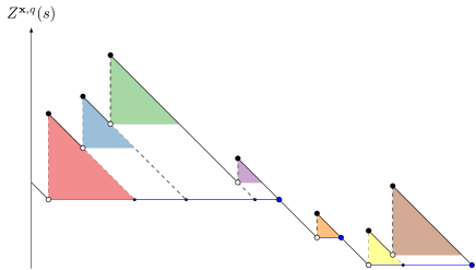
Figure 3: The middle excursion is still in its original (and simplest possible) state: it corresponds to the tree consisting of a single (orange) vertex. The excursion to the right corresponds to a tree with two vertices, and the one to the left corresponds to a tree with four vertices. The dashed lines are added to indicate the triangles, the $i^{\text{th}}$ of which should be matched with vertex $\pi_{i}$.

For $q$ close to $0$ the curve $Z^{\boldsymbol{x},q}$ has only $\operatorname{len}(\boldsymbol{x})$ many (moving) triangular excursions. As $q$ increases, merging gradually happens, and simultaneously (due to the coupling described in previous sections) the excursions of $Z^{\boldsymbol{x},q}$ become more complex. It is interesting to describe here (in Section 3.1.1) the exact structure of this random object, induced by the gradual “pile up” of the original triangles (there are $\operatorname{len}(\boldsymbol{x})$ many in total) on “top of each other”.

The excursion mosaic (or simply the mosaic) is made by drawing at each time $q$ the horizontal (blue in Figure 3) segment on the basis of each excursion of $Z^{\boldsymbol{x},q}$. We call these blue segments active baselines. Furthermore, if the merging of a pair of trees with roots $\pi_{i}$ and $\pi_{j}$ ($i<j$) occurs at time $q$, then

1. the active baseline starting at $\xi_{(i)}^{q}$ is extended until the end of the new (just created by this merging event) excursion at time $q$;

2. the previously (blue) active baseline starting at $\xi_{(j)}^{q}$ turns gray, and it is included in the mosaic at any later time $q+z$ as a segment parallel to the active baseline at the vertical level $Z^{\boldsymbol{x},q+z}(\xi_{(j)}^{q+z}-)$;

3. for each $j\in[\operatorname{len}(\boldsymbol{x})]$, the line indicating the hypotenuse of the $j^{\text{th}}$ successive triangle is extended until it meets the active (blue) baseline of its corresponding excursion.

We call the gray segments from (O.2) the inactive baselines. If clear from the context, we will simply refer to a blue or gray segment as baseline.

From now on, we shall call any excursion of $Z^{\boldsymbol{x},q}$, with its corresponding active and inactive baselines (obtained according to the above given procedure), an ornamented excursion. The ornamented excursions are intended to record the past history of the component mergers in the evolution of the graph. Given this information, it will be possible to construct the surplus edges using an external source of randomness, in a way analogous to the construction in Section 2.2 however adapted to the current setting.

In the next section, we will delve deeper into the ornamented excursions, which is crucial for gaining a comprehensive understanding of these objects. However, it is worth noting that the content of the next section may not be directly relevant to the rest of the paper.

3.1.1 Characterization of the ornamented excursions

If an ornamented excursion of $Z^{\boldsymbol{x},q}$ traverses $\xi_{(k)}^{q}$, we say that it carries $\pi_{k}$. It should be clear that the just given mosaic construction and the related definitions can be transposed so that, for each $q$, the reflected process $B^{\boldsymbol{x},q}$ has the same ornamented excursions as $Z^{\boldsymbol{x},q}$, with the difference that in $B^{\boldsymbol{x},q}$ all the excursions start from the abscissa, i.e. they are all excursions above level $0$.

Note that the ornamented excursions must have some additional “structural” properties, due to their construction and the simultaneous breadth-first walk dynamics. Indeed,

1. for a fixed $q>0$, no two baselines appear on the same level in the same ornamented excursion, almost surely,

2. each gray baseline, as constructed by O.2, must be a continuous segment (it cannot “skip” time intervals),

3. the gray baselines obey a special kind of monotonicity: if $\pi_{j}$ and $\pi_{k}$, where $j<k$, belong to the same ornamented excursion, and if for some $l$ such that $j\leq l\leq k$ the gray baseline at level $Z^{\boldsymbol{x},q}(\xi_{(j)-}^{q})$ intersects the hypotenuse line (described in O.3) corresponding to $\pi_{k}$, then the gray baseline at level $Z^{\boldsymbol{x},q}(\xi_{(j)-}^{q})$ also intersects this hypotenuse line.

Properties O’.1–O’.2 are consequences of the way in which the gray baselines are constructed, see O.2. Furthermore, property O’.3 is a consequence of the breadth-first walk and the coalescent dynamics: a vertex $\pi_{i}$ that coalesces with $\pi_{j}$, such that $j>i$, at time $q$, is immediately connected to all the vertices which were in the connected component of $\pi_{j}$ just prior to time $q$. Furthermore, Figure 4 shows two examples of ill-defined ornamented excursions. Figure 4(a) (resp. 4(b)) does not satisfy O’.2 (resp. O’.3).

(a)

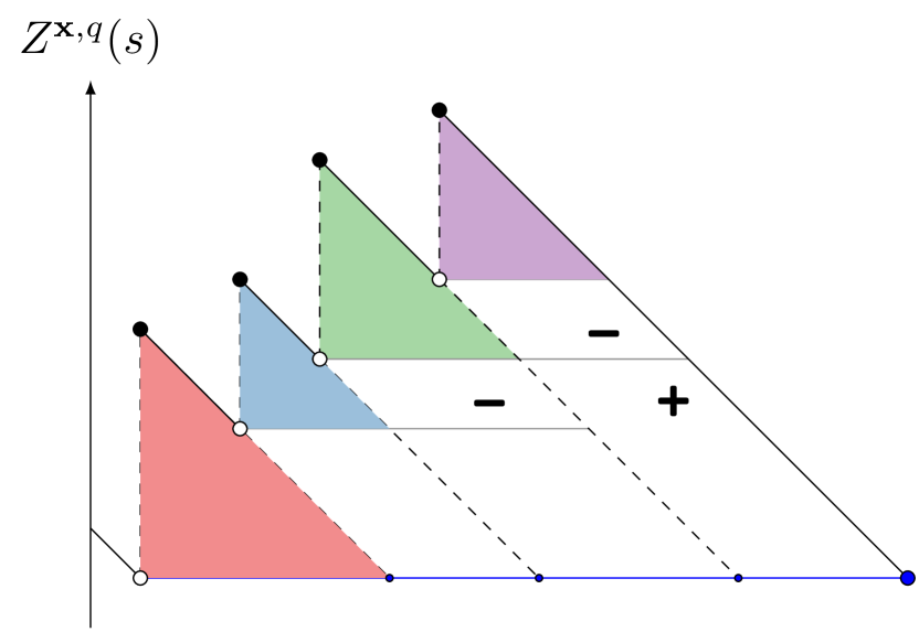
(b)

Figure 4: Two examples of ill-defined ornamented mosaic. In both cases, in order to obtain a well-defined ornamented excursion, either the gray line(s) below the minus sign(s) must be removed, or a gray line below the plus sign must be added.

We will next show that the reverse implication is also true: any excursion ornamented according to the two properties just described (continuity O’.2 and monotonicity O’.3) is a true ornamented excursion, i.e. there exists at least one trajectory of the Aldous’ inhomogeneous continuous-time random graph such that the given ornamented excursion appears at some time $q>0$.

We will illustrate on an example how to construct a trajectory of coalescences in order to obtain a given ornamented excursion. If at a given time $q>0$ there is a non-trivial spanning tree of length four in $\mathcal{F}_{0}$ (or equivalently in $\mathcal{F}_{1}$), then its corresponding ornamented excursion must have one of the five forms depicted in Figure 5. Figure 6 shows the possible trees associated to these five ornamented excursions. The edges completely determined by the ornamented excursions are represented by solid arrows, and those that need to be picked at random according to (6) are represented by dashed arrows.

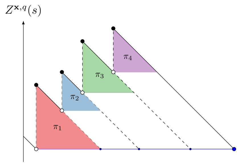
(a)

(b)

(c)

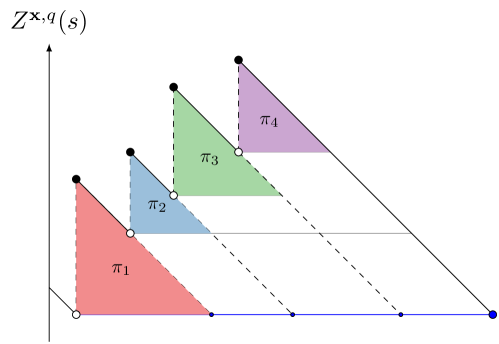
(d)

(e)

Figure 5: The five possible realizations of the excursion mosaic of four vertices, restricted to a single excursion, viewed at a fixed time $q>0$.

(a)

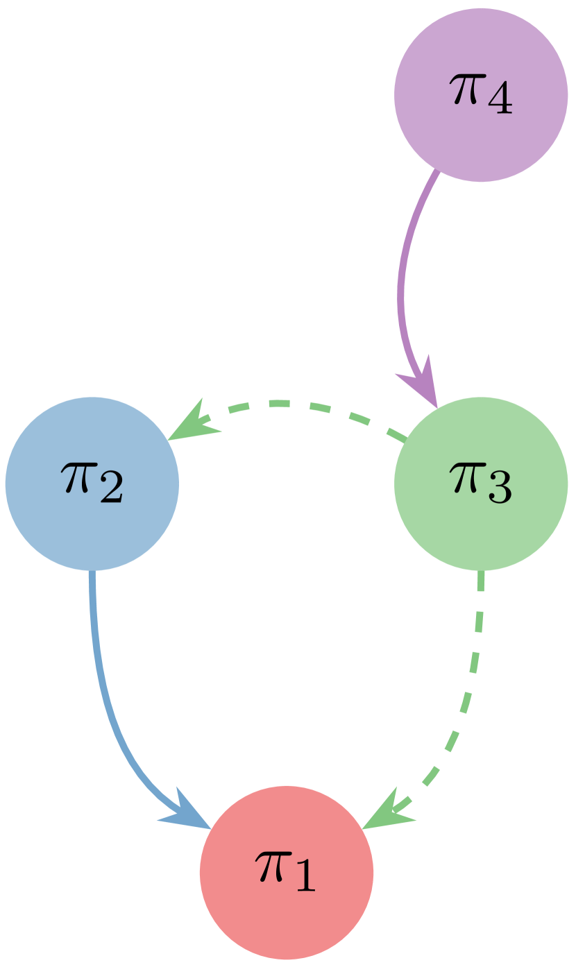
(b)

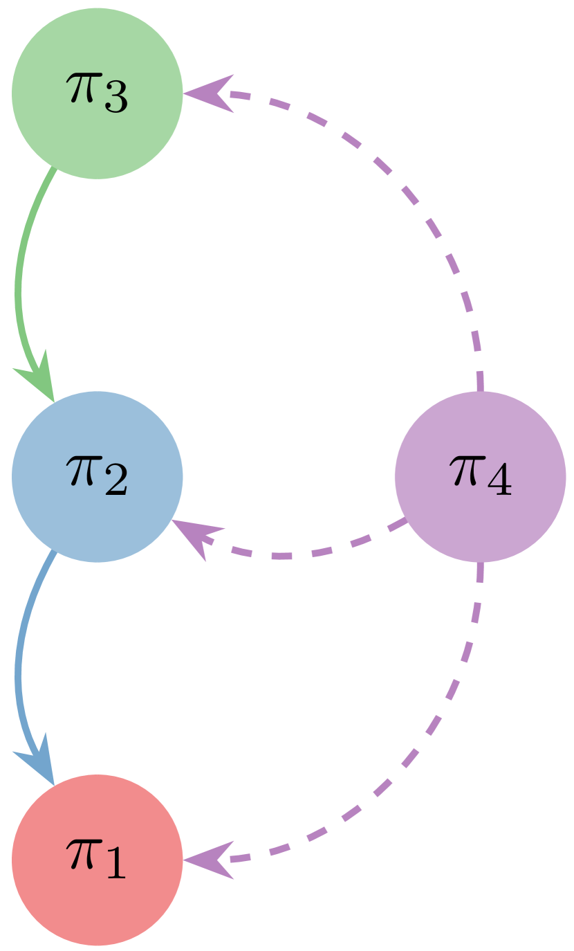
(c)

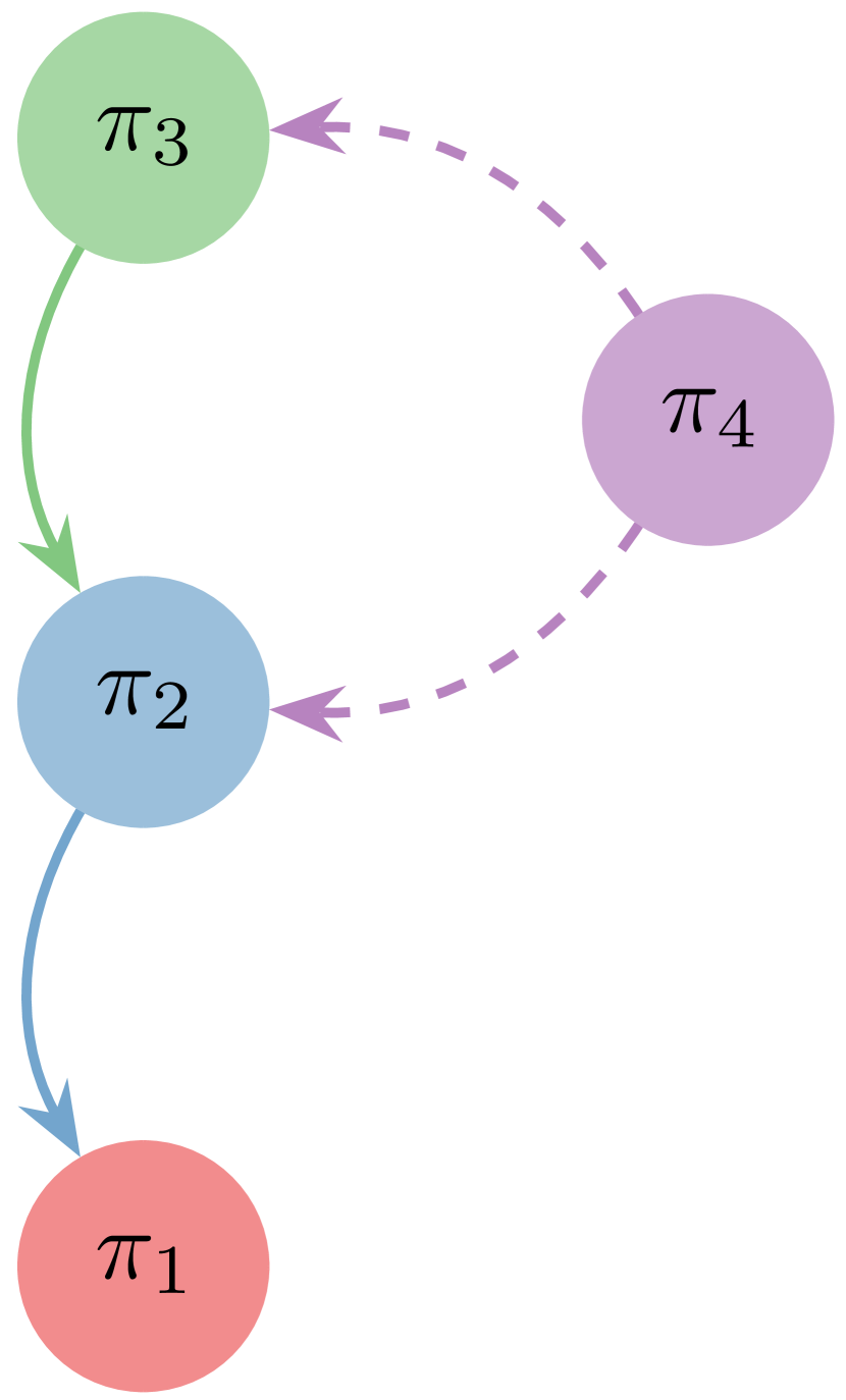
(d)

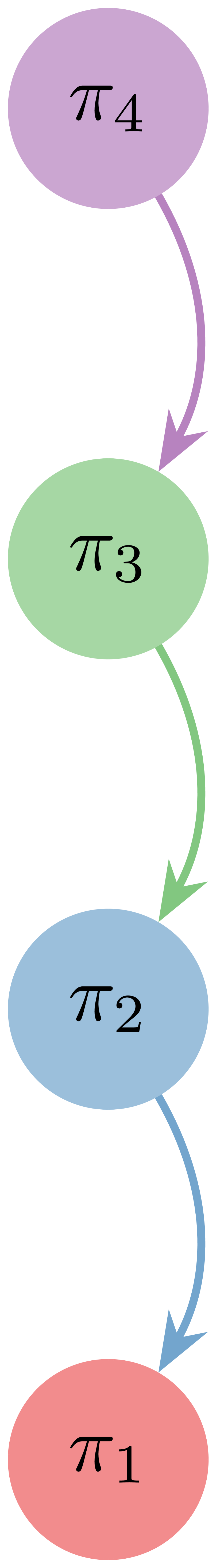
(e)

Figure 6: Representations of the five trees in $\mathcal{F}_{1}$ associated to the five ornamented excursions in Figure 5. A solid arrow indicates an edge in $\mathcal{F}_{1}$ completely specified by the mosaic. The tree corresponding to the fifth image 6(e) (associated to the excursion 5(e)) is completely specified by the mosaic. In the other cases, there is at least one edge (indicated by a dashed arrow) in $\mathcal{F}_{1}$ that needs to be picked via additional randomness. More precisely, for each vertex with dashed arrows issued from it, one of the arrows/edges needs to be picked at random according to (6).

Without loss of generality, we can suppose that at a given time $q>0$ the vertices in the ornamented excursion are precisely $\{\pi_{1},\pi_{2},\dots,\pi_{k}\}$. The ornamented excursion is then completely determined by the order of coalescence of the vertices $\pi_{2},\dots,\pi_{k}$ with their respective immediately closest leftmost neighbors. In the next paragraphs we will describe a construction of a total order on $\{\pi_{2},\dots,\pi_{k}\}$, such that when the vertices coalesce according to the enumeration given by this total order, this results in a given ornamented excursion satisfying O’.2 and O’.3.

Let us first define a partial order $\succeq$ on the set of vertices carried by an ornamented excursion. The leading vertex of the ornamented excursion is the greatest element in the partial order (it is the last element to be visited). In addition, we say that ${\pi_{i}}\succeq{\pi_{j}}$, with $i\leq j$, if $i=j$ or if the gray or blue baseline produced by O.2 and associated to $\pi_{i}$ (if exists) reaches/intersects the hypotenuse line described by O.3 associated to $\pi_{j}$. The assumption of the first vertex in the excursion being the greatest element is compatible with the fact that the corresponding blue baseline (defined in O.1) reaches/intersects any other hypotenuse line, associated to any other vertex carried by the excursion. Note also that O’.3 ensures the transitivity property of the partial order $\succeq$. Even more, if ${\pi_{i}}\succeq{\pi_{j}}$, with $i<j$, then ${\pi_{i}}\succeq{\pi_{k}}$, for every $k$ such that $i\leq k\leq j$. Let us recall that the Hasse diagram associated to the partial order $\succeq$ is the directed graph with edges $\pi_{i}\leftarrow\pi_{j}$ whenever $\pi_{i}\succeq\pi_{j}$ and there is no other $\pi_{k}$ such that $\pi_{i}\succeq\pi_{k}\succeq\pi_{j}$, i.e. if $\pi_{i}$ covers $\pi_{j}$. The Hasse diagram associated to $\succeq$ is consequently a rooted tree whose root is the first element in the excursion, i.e. the greatest element according to $\succeq$. The trees given by the solid arrows in Figure 7 are the Hasse diagrams associated to the partial order $\succeq$ obtained from the excursions in Figure 5.

We now explain how one can use the just mentioned Hasse diagram to decide in which order the vertices $\{\pi_{2},\dots,\pi_{k}\}$ might coalesce to obtain the given ornamented excursion. We define a total order in $\{\pi_{2},\dots,\pi_{k}\}$, denoted by $\succeq^{\star}$, such that if $\pi_{i}$ is in a smaller generation than $\pi_{j}$, in the tree given by the Hasse diagram associated to $\succeq$, then ${\pi_{i}}\succeq^{\star}{\pi_{j}}$. Also, within each generation or level of the Hasse diagram, let us order the vertices according to their index, i.e. $\pi_{i}\succeq^{\star}\pi_{j}$ if $i\geq j$. Then, it is immediate that $\succeq^{\star}$ is a total order in the set of vertices carried by the excursion. Figure 7 shows the Hasse diagrams associated to the total order $\succeq^{\star}$ for the five excursions in Figure 5, with dashed arrows indicating the order of coalescence. Let us show that merging of the vertices according to the total order just defined will produce the given ornamented excursion. Indeed, assume that according to the order $\succeq^{\star}$, we are about to merge the excursion carrying $\pi_{i}$ with the excursion carrying $\pi_{i-1}$. By construction, the subtree rooted in $\pi_{i}$ contains precisely all the vertices $\pi_{j}$, with $j\geq i$, such that $\pi_{i}\succeq\pi_{j}$, i.e. exactly those vertices whose hypotenuse gray lines are reached by the blue (to become gray) baseline associated to $\pi_{i}$. Furthermore, any vertex $\pi_{k}$ in the same generation of the Hasse diagram as $\pi_{i}$, but such that $i>k$, i.e. such that $\pi_{i}\succeq^{\star}\pi_{k}$, must not be contained in the excursion carrying $\pi_{i-1}$ at the time of this merger event.

Due to the above reasoning, the coalescence of $\pi_{i}$ produces exactly the gray baseline in the given ornamented excursion. Note that coalescing the vertices in a different order than the one induced by $\succeq^{\star}$ could produce undesired gray baselines. Indeed, for two vertices such that $\pi_{i}\succeq^{\star}\pi_{k}$ and $i>k$, the coalescence of vertex $\pi_{i}$ before $\pi_{k}$, could produce a gray baseline associated to $\pi_{k}$ longer than that in the given ornamented excursion. See, for instance, the difference between the Hasse diagrams in Figures 7(d) and 7(e) related to the ornamented excursions in Figures 5(d) and 5(e), respectively, focusing on $i=4$ and $k=3$.

The total orders induced by $\succeq^{\star}$ (dashed arrows) associated to the ornamented excursions in Figure 5 and represented by the Hasse diagrams in Figure 7 are summarized in Table 1. Notice that, even though the total order defined for a given ornamented excursion is a natural choice, it is not the only ordering of coalescence of vertices resulting in the given ornamented excursion. It can be easily checked that the total order $\pi_{3}\succeq^{\star}\pi_{4}\succeq^{\star}\pi_{2}$, which is not listed in Table 1, also produces the ornamented excursion in Figure 5(b).

Hasse diagram	Total order
Figure 7(a)	$\pi_{4}\succeq^{\star}\pi_{3}\succeq^{\star}\pi_{2}$
Figure 7(b)	$\pi_{3}\succeq^{\star}\pi_{2}\succeq^{\star}\pi_{4}$
Figure 7(c)	$\pi_{4}\succeq^{\star}\pi_{2}\succeq^{\star}\pi_{3}$
Figure 7(d)	$\pi_{2}\succeq^{\star}\pi_{4}\succeq^{\star}\pi_{3}$
Figure 7(e)	$\pi_{2}\succeq^{\star}\pi_{3}\succeq^{\star}\pi_{4}$

Table 1: Total order induced by the ornamented excursions in Figure 5, whose Hasse diagrams are represented by dashed arrows in Figure 7.

Figure 9(a) shows a more complicated ornamented excursion carrying eight vertices. Figure 9(b) shows the associated tree where, similarly to Figure 6, the edges completely determined by the excursion are represented by solid arrows and those that need to be picked according to (6) are represented by dashed arrows. Also, Figure 9(c) shows the respective Hasse diagrams associated to the orders $\succeq$ and $\succeq^{\star}$ defined on the set of vertices (excluding the root), with solid and dashed arrows, respectively.

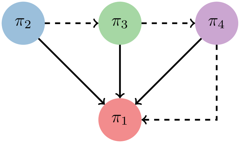
(a)

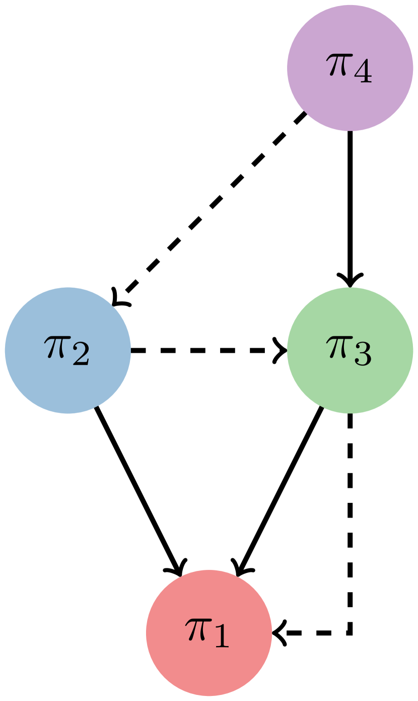
(b)

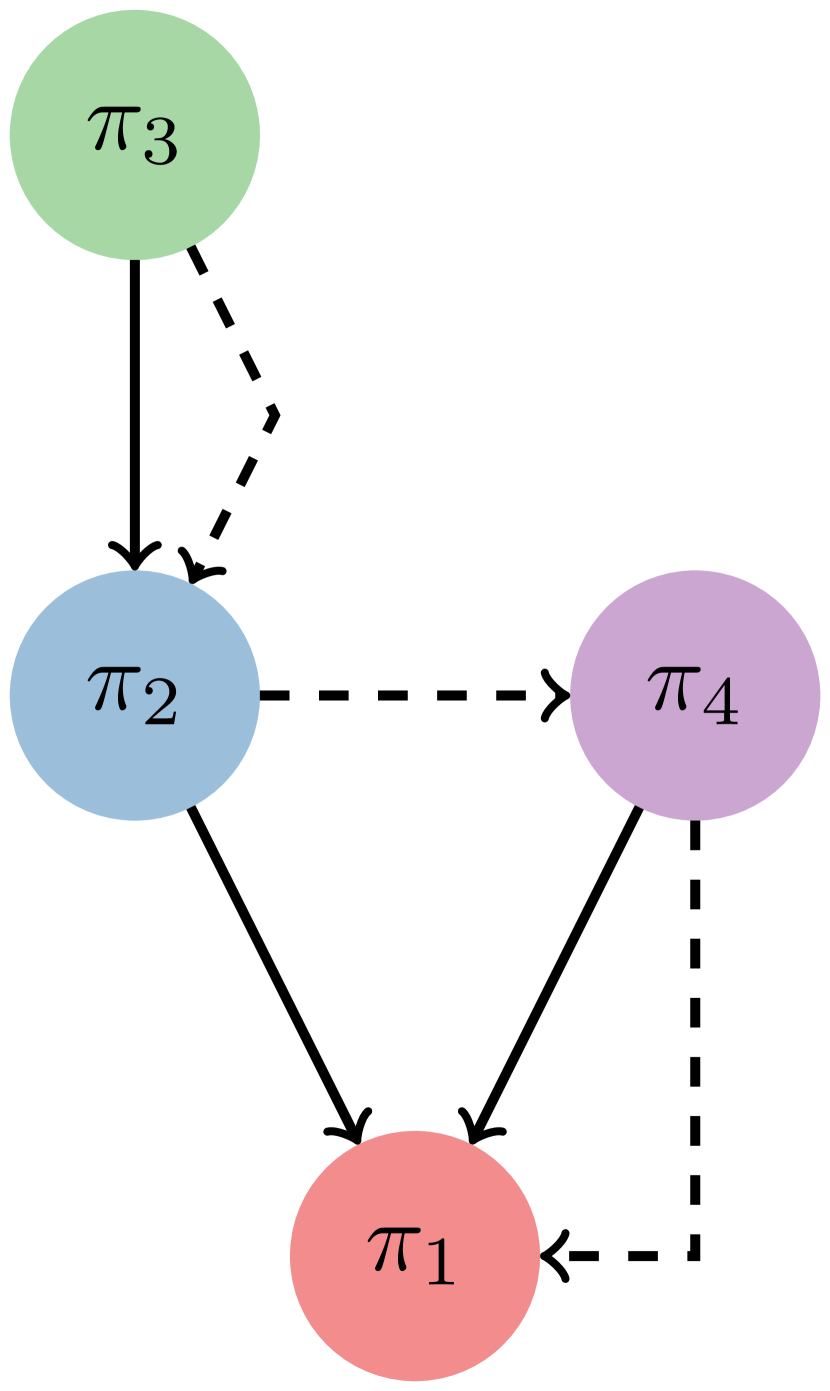
(c)

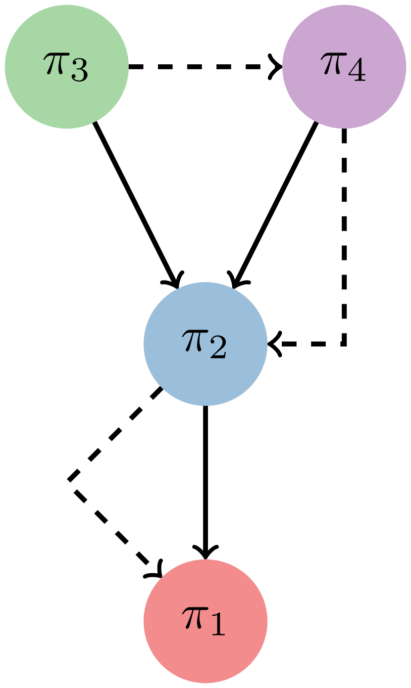
(d)

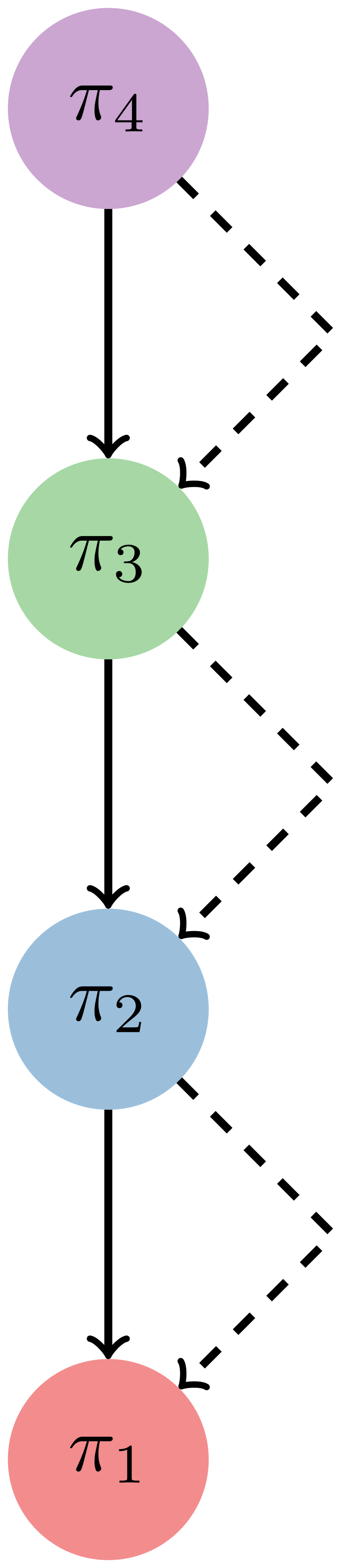
(e)

Figure 7: The tree formed by the solid (resp. dashed) arrows is the Hasse diagram associated to the partial order $\succeq$ (resp. total order $\succeq^{\star}$). Collapsing the nodes according to the paths defined by the dashed arrows will produce the ornamented excursions in Figure 5.

3.1.2 The surplus edges dynamic

Let us first show on an example how the surplus edges can be superimposed in a consistent way. Consider the Figure 5(b). Let us enumerate the four parallelograms specified by the mosaic in some way, for example traverse them row-by-row from left to right, as an analogue to the breadth-first order (see Figure 1). Let $\zeta^{2;1}$, $\zeta^{3;2,1}$, $\zeta^{4;2,1}$ and $\zeta^{4;3}$ be independent Poisson point processes (PPP), matched respectively to these four regions, as shown in Figure 8.

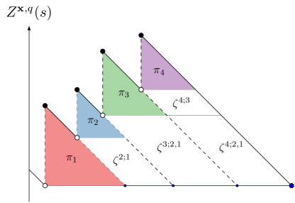
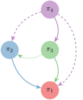
Figure 8: The excursion is the same as in Figure 5(b). In the tree, it is assumed that the edges $\pi_{4}\to\pi_{3}$ and $\pi_{3}\to\pi_{1}$ were sampled according to (6) and thus included in $\mathcal{F}_{1}$. The four independent PPP $\zeta^{2;1}$, $\zeta^{3;2,1}$, $\zeta^{4;2,1}$ and $\zeta^{4;3}$, with rates $x_{\pi_{2}}\cdot x_{\pi_{1}}$, $x_{\pi_{3}}(x_{\pi_{2}}+x_{\pi_{1}})$, $x_{\pi_{4}}(x_{\pi_{2}}+x_{\pi_{1}})$ and $x_{\pi_{4}}\cdot x_{\pi_{3}}$, respectively, are matched to the four parallelogram regions as shown in the excursion. The dotted green arrow represents the surplus edge that will be created using $\zeta^{3;2,1}$ and the dashed violet arrows represent the surplus edges that will be created using $\zeta^{4;2,1}$.

As $q$ increases, for each of the parallelograms its base stays fixed in length (although it moves closer to the origin), and its height increases. Let a point arrive to $\zeta^{2;1}$ at rate $x_{\pi_{2}}\cdot x_{\pi_{1}}$, to $\zeta^{3;2,1}$ at rate $x_{\pi_{3}}(x_{\pi_{2}}+x_{\pi_{1}})$, to $\zeta^{4;2,1}$ at rate $x_{\pi_{4}}(x_{\pi_{2}}+x_{\pi_{1}})$, and to $\zeta^{4;3}$ at rate $x_{\pi_{4}}\cdot x_{\pi_{3}}$. As it turns out, most of these Poisson point processes will not be needed now, but they are nevertheless defined with an intention of later use. Let us assume that, due to randomization (6), the realization of the corresponding random tree has the following three edges: $\pi_{2}\rightarrow\pi_{1}$, $\pi_{3}\rightarrow\pi_{1}$, and $\pi_{4}\rightarrow\pi_{3}$, as shown in Figure 8. We only need to watch for marks in $\zeta^{3;2,1}$ and $\zeta^{4;2,1}$. When a new mark arrives to $\zeta^{3;2,1}$, with probability $x_{\pi_{2}}/(x_{\pi_{1}}+x_{\pi_{2}})$ the process creates an edge $\pi_{3}\rightarrow\pi_{2}$, unless this edge already exists. This surplus edge is represented by a dotted arrow in Figure 8. Nothing happens with the remaining probability. When a new mark arrives to $\zeta^{4;2,1}$, with probability $x_{\pi_{2}}/(x_{\pi_{1}}+x_{\pi_{2}})$ (resp. $x_{\pi_{1}}/(x_{\pi_{1}}+x_{\pi_{2}})$) the process creates an edge $\pi_{4}\rightarrow\pi_{2}$ (resp. $\pi_{4}\rightarrow\pi_{1}$), unless it already exists. These surplus edges are represented by dashed arrows in Figure 8. It is likely clear to the reader that these transitions are chosen with the purpose of preserving the random graph transitions within the connected components.

In the general case, one has the collection of Poisson processes $\zeta^{l;j-k}$, where $j,k,l$ run over all the indices in $[\operatorname{len}(\boldsymbol{x})]$ such that

$$j\leq k\leq l,\mbox{ and if }k=l\mbox{ then also }j=l.$$ (7)

The processes $(\zeta^{l;l-l})_{l}$ play a special role, to be explained in Section 3.2. If $l>k$, then $\zeta^{l;j-k}$ is in charge of generating a surplus edge from $\pi_{l}$ to some vertex in the range $\{\pi_{j},\ldots,\pi_{k}\}$, but only when compatible with the excursion mosaic. More precisely, $\zeta^{l;j-k}$ will be active starting from the time $T_{l;j-k}$ at which the ornamented excursion of $Z^{\boldsymbol{x},\cdot}$ carrying $\pi_{l}$ (as its root or a non-root vertex) merges with an ornamented excursion carrying precisely $\{\pi_{j},\ldots,\pi_{k}\}$. In this way, the random time $T_{l;j-k}$ depends on the mosaic, and it is finite if and only if the just described merging configuration occurs. It can happen that $j=k<l$, in the case where the ornamented excursion carrying $\pi_{l}$ (with leading vertex $\pi_{j+1}$) merges with a simple triangular excursion carrying only $\pi_{j}$. On the event $\{T_{l;j-k}=\infty\}$, the corresponding $\zeta^{l;j-k}$ is never activated. On $\{T_{l;j-k}<\infty\}$, the behavior of $\zeta^{l;j-k}$ after $T_{l;j-k}$ is a generalization of the one given in the example above (see e.g. $\zeta^{3;2,1}$). More precisely, the points arrive to $\zeta^{l;j-k}$ at rate $x_{\pi_{l}}(x_{\pi_{j}}+\ldots+x_{\pi_{k}})$. The first (spanning) edge is created according to (6) when the merging occurs. The surplus edges are created as follows: given an arrival to $\zeta^{l;j-k}$ at time $q>T_{l;j-k}$, an index $I$ is drawn (independently of the past of the mosaic, of $\mathcal{F}_{1}$, and of the surplus edge data), so that $I=i$ with probability $x_{\pi_{i}}/(x_{\pi_{j}}+\ldots+x_{\pi_{k}})$ for each $i\in\{j,\ldots,k\}$. Given $I$, the surplus edge $l\rightarrow I$ is created, unless it already exists. For each $q>0$, call any edge created in this way before time $q$ a surplus edge arriving before $q$. Let $G_{1}^{\boldsymbol{x}}(q)=(V,E_{1}(q))$, where $E_{1}(q)$ is the union of the spanning edges in $\mathcal{F}_{0}(q)$ and surplus edges arriving before $q$. Then it is clear that $G_{1}^{\boldsymbol{x}}$ is a monotone random graph process: $G_{1}^{\boldsymbol{x}}(q_{1})\subset G_{1}^{\boldsymbol{x}}(q_{2})$ whenever $q_{1}\leq q_{2}$. In fact, we have derived a stronger claim, that may serve as the main motivation for the extra construction presented in the next section.

Theorem 3.2.

For any general initial positive weights $\boldsymbol{x}$, the just constructed graph-valued process $(G_{1}^{\boldsymbol{x}}(q),\,q\geq 0)$ is a realization of the Aldous’ (inhomogeneous) continuous-time random graph $(\mathcal{G}^{\boldsymbol{x}}(q),q\geq 0)$.

3.2 Proof of Theorem 1.1

Here we focus on the second construction above (see Section 3.1). In particular, recall the excursion mosaic, and the family of compatible Poisson point processes $\zeta^{l;j-k}$, where $j,k,l$ satisfy the constraints given in (7). For each $l$, $\zeta^{l;l-l}$ should now be matched at time $q$ to the triangle spanned by the points $(\xi_{(l)}^{q},Z^{\boldsymbol{x},q}(\xi_{(l)}^{q}-))$, $(\xi_{(l)}^{q},Z^{\boldsymbol{x},q}(\xi_{(l)}^{q}))$ and $(\xi_{(l)}^{q}+x_{\pi_{l}},Z^{\boldsymbol{x},q}(\xi_{(l)}^{q}-))$ (or equivalently, to that spanned by $(\xi_{(l)}^{q},B^{\boldsymbol{x},q}(\xi_{(l)}^{q}-))$, $(\xi_{(l)}^{q},B^{\boldsymbol{x},q}(\xi_{(l)}^{q}))$ and $(\xi_{(l)}^{q}+x_{\pi_{l}},B^{\boldsymbol{x},q}(\xi_{(l)}^{q}-))$). This Poisson point process is active already at time $0$ (the triangular excursions exist from the very beginning). We therefore define $T_{l;l-l}\equiv 0$ almost surely, for each $l\in[\operatorname{len}(\boldsymbol{x})]$. Points arrive to $\zeta^{l;l-l}$ at rate $x_{\pi_{l}}^{2}/2$, and at the time of each arrival, a self-loop $\pi_{l}\rightarrow\pi_{l}$ is created.

Remark 3.3.

The factor of $1/2$ is natural if one thinks of each original block as continuous “spread” of mass, and of each self-loop as an edge between two different points in this block. If $x$ is discretized into $n$ subblocks of equal mass $x/n$ for some large $n$, and if an edge between the $i^{\text{th}}$ and the $j^{\text{th}}$ subblock arrives at the multiplicative rate $(x/n)^{2}$, then the total rate of edge arrivals equals $(x/n)^{2}\cdot{n\choose 2}=\frac{x^{2}}{2}(1-1/n)\approx x^{2}/2$. Not surprisingly, this rate is also the area of the triangle to which $\zeta^{l;l-l}$ is matched.

As in Section 3.1, for $l>k$ the counting process $\zeta^{l;j-k}$ is activated at time $T_{l;j-k}$, hence never on $\{T_{l;j-k}=\infty\}$. After activation, the points arrive to $\zeta^{l;j-k}$ again at rate $x_{\pi_{l}}(x_{\pi_{j}}+\ldots+x_{\pi_{k}})$. The surplus multi-edges are created as before, but without an additional “lack of previous presence” constraint: given an arrival to $\zeta^{l;j-k}$ at time $q$, an index $I$ is drawn in the same way as before, and a new surplus (multi-)edge $l\rightarrow I$ is created at time $q$. The multi-graph obtained in this way follows the same distribution as $(\mathcal{MG}^{\boldsymbol{x}}(q),q\geq 0)$.

It was already explained how $\zeta^{l;l-l}$ can be matched to the $l^{\text{th}}$ triangular region under the curve $B^{\boldsymbol{x},\cdot}$. It is useful to point out here that $\zeta^{l;j-k}$ (on $\{T_{l;j-k}<\infty\}$) can analogously be matched to a parallelogram shaped region (evolving in time) on the ornamented mosaic, for any choice of $l>k\geq j$ such that $\zeta^{l;j-k}$ gets activated. Before time $T_{l;j-k}$ this parallelogram does not exist, exactly at time $T_{l;j-k}$ it has height $0$, and its height (strictly) increases at any future time. Indeed, this parallelogram of constant base length $x_{\pi_{l}}$ is created at time $T_{l;j-k}$ by the excursion mosaic, and at any time $z>T_{l;j-k}$ it is the region specified by the four lines

$$\begin{array}[]{ll}y=-\left(x-\xi_{(l)}^{z}\right)+Z^{\boldsymbol{x},z}\left(\xi_{(l)}^{z}-\right)&\ \mbox{\small{``left'' boundary}},\\ y=Z^{\boldsymbol{x},z}\left(\xi_{(j)}^{z}-\right)&\ \mbox{\small{``bottom'' boundary}},\\ y=-\left(x-\xi_{(l)}^{z}\right)+Z^{\boldsymbol{x},z}\left(\xi_{(l)}^{z}\right)&\ \mbox{\small{``right'' boundary}},\\ y=Z^{\boldsymbol{x},z}\left(\xi_{(j_{1})}^{z}-\right)&\ \mbox{\small{``top'' boundary}},\\ \end{array}$$ (8)

where $j_{1}=k+1$.

Remark 3.4.

Let us note (as easily derived from the construction) that $j_{1}=k+1$ almost surely on $\{T_{l;j-k}<\infty\}$, since the excursion carrying $\pi_{l}$ must have $\pi_{k+1}$ as its leading vertex (or equivalently, $\pi_{k+1}$ is the root of the corresponding spanning tree) just prior to the merger.

Figure 9 shows how the mosaic drawn in previous figures might look at a later time. For the sake of illustration, let us assume that the eight jumps (vertices) in Figure 9 are $\pi_{3},\ldots,\pi_{10}$, where $\pi_{3}$ is indicated in yellow, and $\pi_{10}$ in orange (the jumps at $\xi_{(1)}^{q}$ and at $\xi_{(2)}^{q}$ are not contained in the plot region).

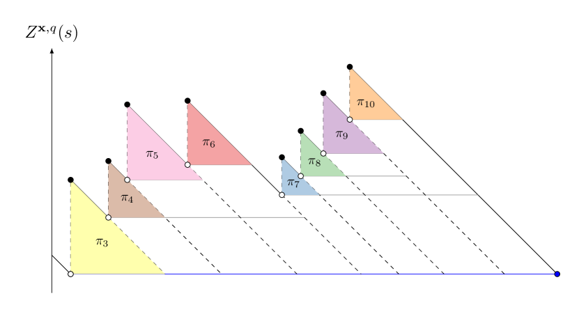
(a)

(b)

(c)

Figure 9: The tree 9(b) associated to the ornamented excursion 9(a) is partially determined by the mosaic. The dashed edges in 9(b) indicate various options, to be decided according to (6). The solid arrows in 9(c) are the edges in the Hasse diagram related to the order $\succeq$ associated to the ornamented excursion 9(a), as described in Section 3.1.1. The dashed arrows in 9(c) represent the Hasse diagram of the total order $\succeq^{\star}$, also defined in Section 3.1.1. For the violet vertex $\pi_{9}$, there are three active Poisson point processes $\zeta^{9;8-8}$, $\zeta^{9;7-7}$ and $\zeta^{9;3-6}$ running at that time. For the orange vertex $\pi_{10}$, there are only two active Poisson point processes $\zeta^{10;7-9}$, and $\zeta^{10;3-6}$ running. The process $\zeta^{9;7-7}$ corresponds to the middle parallelogram in the “$\pi_{9}$-slice”, containing the triangle marked in violet, and $\zeta^{10;3-6}$ corresponds to the lower parallelogram in the “$\pi_{10}$-slice”, containing the triangle marked in orange. There is no $\zeta^{7;3-5}$, why? Find $\zeta^{6;3-3}$ and $\zeta^{6;4-5}$.

The excursion mosaic is an object of interest due to the following claim in particular.

Proposition 3.3.

For any choice of $j,k,l$ specified in (7), and for any fixed $q$, on $\{T_{l;j-k}\leq q\}$, the cumulative arrival rate to $\zeta^{l;j-k}$ up to time $q$ equals almost surely the area of the region in the excursion mosaic matched to $\zeta^{l;j-k}$ at time $q$, multiplied by $q$.

Proof.

If $j=k=l$, the statement is trivial to check. Suppose that $l>k$, so that the corresponding region in the mosaic is a parallelogram. Then clearly the total arrival rate to $\zeta^{l;j-k}$ before time $q$ equals $(q-T_{l;j-k})\cdot x_{\pi_{l}}(x_{\pi_{j}}+\ldots+x_{\pi_{k}})$.

Abbreviate

$$\Xi:=x_{\pi_{j}}+\ldots+x_{\pi_{k}}.$$

Then the total rate above can be rewritten as

$$q\left(\Xi-\Xi\cdot\frac{T_{l;j-k}}{q}\right)\cdot x_{\pi_{l}}.$$

The claim we need to prove is therefore identical to the fact that the height of the parallelogram specified in (8) equals the term in parentheses. Recall Remark 3.4. At time $q$, the height of the parallelogram from (8) is

$$Z^{\boldsymbol{x},q}\left(\xi_{(k+1)}^{q}-\right)-Z^{\boldsymbol{x},q}\left(\xi_{(j)}^{q}-\right)\equiv\Xi-\frac{\xi_{(k+1)}-\xi_{(j)}}{q}.$$ (9)

It was already noted that $T_{l;j-k}$ (whenever finite) is the time of merging of two excursions (one carrying $\pi_{l}$ and the other carrying exactly $\pi_{j},\ldots,\pi_{k}$ immediately prior to $T_{l;j-k}$). Recalling Remark 3.4 again, we conclude that the time $T_{l;j-k}$ of merging of these two excursions must satisfy the identity

$$\xi_{(k+1)}-\xi_{(j)}=\Xi\cdot T_{l;j-k}.$$ (10)

By plugging in (10) into (9), it is simple to verify that on $\{T_{l;j-k}\leq q\}$ the quantity $Z^{\boldsymbol{x},q}\left(\xi_{(k+1)}^{q}-\right)-Z^{\boldsymbol{x},q}\left(\xi_{(j)}^{q}-\right)$ equals $\Xi\cdot(1-T_{l;j-k}/{q})$, almost surely, which is the required identity. ∎

We shall refer to the bounded (random) region specified by the lines

$$\begin{array}[]{ll}y=-\left(x-\xi_{(l)}^{z}\right)+B^{\boldsymbol{x},z}\left(\xi_{(l)}^{z}-\right)&\ \mbox{\small{``left lower'' boundary}},\\ x=\xi_{(l)}^{z},&\ \mbox{\small{``left upper'' boundary}}\\ y=-\left(x-\xi_{(l)}^{z}\right)+B^{\boldsymbol{x},z}\left(\xi_{(l)}^{z}\right)&\ \mbox{\small{``right'' boundary}},\\ y=0&\ \mbox{\small{``bottom'' boundary}},\\ \end{array}$$

as the $\pi_{l}$-slice (under the curve of $B^{\boldsymbol{x},q}$). From the discussion above, we see that the $\pi_{l}$-slice is split by the mosaic into the right isosceles triangle of area $(x_{\pi_{l}})^{2}/2$ and (possibly) additional parallelograms, each of which corresponds to $\zeta^{l;j-k}$ for some $j\leq k<l$ such that $T_{l;j-k}\leq q$. In this way, the region under the excursion of $B^{\boldsymbol{x},z}$ carrying exactly $\pi_{h},\pi_{h+1},\ldots,\pi_{h+r}$ at time $q$ is the union of the $\pi_{h}$-slice, the $\pi_{h+1}$-slice, $\ldots$, and the $\pi_{h+r}$-slice. The intersections of adjacent regions and slices are sets (segments) of zero Lebesgue measure. Thus, the cumulative rate of (oriented) surplus edges issued from $\pi_{l}$ before time $q$ is the area of $\pi_{l}$-slice at time $q$, multiplied by $q$. This leads to the next result.

Lemma 3.4 (Area below the excursion and surplus edges).

The cumulative rate of surplus edges in the component of $\mathcal{MG}^{\boldsymbol{x}}(q)$ consisting of $\pi_{h},\pi_{h+1},$ $\ldots,\pi_{h+r}$ is the area of the excursion of $B^{\boldsymbol{x},q}$ carrying exactly $\pi_{h},\pi_{h+1},\ldots,\pi_{h+r}$, multiplied by $q$.

Using Lemma 3.4, the proof of Theorem 1.1 simply follows from elementary properties of the construction of $\big{(}\boldsymbol{X}^{\boldsymbol{x}}(q),\boldsymbol{N}^{\boldsymbol{x}}(q)\big{)}$ defined by (3). Indeed, the number of points of the Poisson point process $\Lambda$ lying below the curve $s\mapsto q\cdot B^{\boldsymbol{x},q}(s)$ over different excursions are conditionally independent. This means that, in addition to the information on the size of the connected components of $\mathcal{MG}^{\boldsymbol{x}}(q)$, the reflected simultaneous breadth-first walk $B^{\boldsymbol{x},q}$ also encodes the information on the cumulative rate of surplus edges, which is the area below the curve of the corresponding excursion.

4 Related results and open problems

Define the parameter space

$$\mathcal{I}:=\big{(}(0,\infty)\times(-\infty,\infty)\times l^{3}_{\searrow}\big{)}\cup\big{(}\{0\}\times(-\infty,\infty)\times l^{3}_{\searrow}\setminus l^{2}_{\searrow}\big{)}.$$

Let $(\kappa,\tau,\boldsymbol{c})\in\mathcal{I}$. Given a family $(\xi_{j}^{\prime})_{j}$ of independent exponential random variables, where $\xi_{j}^{\prime}$ has rate $c_{j}$, define

$$V^{\boldsymbol{c}}(s)=\sum_{j}\left(c_{j}\cdot\mathbb{1}_{(\xi_{j}^{\prime}\leq s)}-c_{j}^{2}\cdot s\right),\ s\geq 0.$$

For each $t\in\mathbb{R}$, let

$$W^{\kappa,t-\tau,\boldsymbol{c}}(s)=\kappa^{1/2}W(s)-\tau s-\frac{1}{2}\kappa s^{2}+V^{\boldsymbol{c}}(s)+ts,\ s\geq 0,$$

where $W$ is standard Brownian motion, and $W$ and $V^{\boldsymbol{c}}$ are independent, and let

$$B^{\kappa,t-\tau,\boldsymbol{c}}(s):=W^{\kappa,t-\tau,\boldsymbol{c}}(s)-\min_{0\leq s^{\prime}\leq s}W^{\kappa,t-\tau,\boldsymbol{c}}(s^{\prime}),\ s\geq 0.$$ (11)

For a given $\boldsymbol{x}\in l^{2}_{\searrow}$ let $\sigma_{r}(\boldsymbol{x}):=\sum_{i}x_{i}^{r},\text{ for }r=1,2,3.$ Assume that the sequence of initial masses $(\boldsymbol{x}^{(n)})_{n}$ satisfy the following conditions:

$$\frac{\sigma_{3}\left(\boldsymbol{x}^{(n)}\right)}{\left(\sigma_{2}\left(\boldsymbol{x}^{(n)}\right)\right)^{3}} \rightarrow\kappa+\sum_{j}c_{j}^{3},$$ (12)

$$\frac{x_{j}^{(n)}}{\sigma_{2}\left(\boldsymbol{x}^{(n)}\right)} \rightarrow c_{j},\quad j\geq 1,$$ (13)

$$\sigma_{2}\left(\boldsymbol{x}^{(n)}\right) \rightarrow 0,$$ (14)

as $n\to\infty$. It is always possible to find sequences $\big{(}\boldsymbol{x}^{(n)}\big{)}_{n\geq 1}$ satisfying (12) (13) and (14), for every $(\kappa,0,\boldsymbol{c})\in\mathcal{I}$, see [AL98, Lemma 8].

For each $t$, let $\mathcal{X}(t)=\mathcal{X}^{\kappa,\tau,\boldsymbol{c}}(t)$ be the infinite vector of ordered excursion lengths of $B^{\kappa,t-\tau,\boldsymbol{c}}$ away from $0$. Theorem 1.2 in [Lim19] says that the process $(\mathcal{X}(t),t\in(-\infty,\infty))$ is a realization of the extreme eternal multiplicative coalescent corresponding to $(\kappa,\tau,\boldsymbol{c})\in\mathcal{I}$. Furthermore, Corollary 11 in [Lim19] says $\mathcal{X}(t)$ is the scaling limit of the multiplicative coalescent started from $\boldsymbol{x}^{(n)}$ (satisfying (12), (13) and (14)), observed at time $q_{n}(t)=t+1/\sigma_{2}(\boldsymbol{x}^{(n)})$, when $n\to\infty$.

Theorem 1.1 and Remarks 2.1 and 2.2 are promising in view of novel scaling limits for near-critical random graphs, outside the domain of attraction of the Aldous standard multiplicative coalescent. The eternal standard augmented multiplicative coalescent is the original one of Bhamidi et al. [BBW14], a version of which was constructed in [BM16] as the scaling limit of the random graph with surplus counts for special initial configurations of the form

$$x_{1}=x_{2}=\ldots=x_{n}=1/n^{2/3},\text{ and }0=x_{n+1}=\ldots,\text{ as }n\text{ diverges.}$$ (15)

Also, Dhara et al. [DvdHvLS17, Thm. 3.6] obtained a version of the eternal standard augmented multiplicative coalescent for configuration models with finite third moment degrees. Furthermore, [DvdHvLS20, Thm. 2 and 5] found the scaling limit for the sizes of the connected components and the number of surplus edges for configuration models with heavy-tailed distribution in the degree. In this latter setting, the version of the augmented multiplicative coalescent that appears is not the standard one, instead it is the one where the Brownian part vanishes, (i.e.  $\kappa=0$ and $\boldsymbol{c}\in l^{3}_{\searrow}\setminus l^{2}_{\searrow}$). At present, as far as we know, these are the only versions of the augmented multiplicative coalescent that have been studied.

The existence of the standard augmented multiplicative coalescent as the scaling limit of the Erdős – Rényi random graph (i.e. as in (15)) was recently revisited by the authors in the companion paper [CL23]. Our new proof is based on some of the results in this paper, and Theorem 1.1 in particular. The construction exhibited in [CL23] is self-contained (modulo Theorem 1.1), and it is simpler and more direct and than any construction previously available in the literature. In addition, we believe that the methods used in [CL23] could be extended for proving existence of other (non-standard) augmented multiplicative coalescent, as we anticipate in Conjecture 4.1 below.

Let $\Lambda$ be a homogeneous Poisson point process on $[0,\infty)\times[0,\infty)$, independent of $\sigma\{W,V^{\boldsymbol{c}}\}$. In analogy to [Ald97, BBW14], let $\Lambda^{\kappa,t-\tau,\boldsymbol{c}}(s)$ be the number of points in $\mathcal{N}$ below the curve $u\mapsto B^{\kappa,t-\tau,\boldsymbol{c}}(u)$, $u\in[0,s]$. To each excursion of $B^{\kappa,t-\tau,\boldsymbol{c}}$ above $0$, one can assign a random “mark count” to be the increase in $\Lambda^{\kappa,t-\tau,\boldsymbol{c}}$ attained during this excursion (see [BBW14, Section 2.3.2] for details). Let $\mathcal{N}_{i}(t)$ be this count corresponding to the $i^{\text{th}}$ longest excursion of $B^{\kappa,t-\tau,\boldsymbol{c}}$, and $\mathcal{N}(t)=\mathcal{N}^{\kappa,\tau,\boldsymbol{c}}(t)=(\mathcal{N}_{1}(t),\mathcal{N}_{2}(t),\ldots)$. Given the observations made in previous sections, the following can be anticipated (a work in progress by the authors is devoted the proof of this claim):

Conjecture 4.1.

Fix a $(\kappa,\tau,\boldsymbol{c})\in\mathcal{I}$. Then $(\mathcal{X}(t),\mathcal{Y}(t))$, $\,-\infty<t<\infty)$ is a càdlàg realization of the eternal augmented multiplicative coalescent corresponding to $(\kappa,\tau,\boldsymbol{c})$. Furthermore, $((\mathcal{X}(t),\mathcal{Y}(t))$, $\,-\infty<t<\infty)$ is the simultaneous scaling limit of near-critical random graph component sizes and surplus counts, under the hypotheses of the initial configurations (12), (13) and (14).

In addition, the extreme eternal augmented multiplicative coalescents are only the constant ones, and the non-trivial ones given here (corresponding to valid parameters $(\kappa,\tau,\boldsymbol{c})$). Any eternal augmented multiplicative coalescent is a mixture of extreme ones.

The excursion mosaic and the accompanying PPP family $\zeta^{l;j-k}$, $j\leq k\leq l$ (see Section 3.1) has a much richer structure than the mere component sizes superimposed by surplus edge counts. Is there a natural framework and candidate for its scaling limit in the near-critical regime(s)? This insight would surely encompass a clearer understanding of mark counts $\mathcal{N}$ in the eternal augmented coalescent.

References

- [AL98] D. Aldous and V. Limic, The entrance boundary of the multiplicative coalescent, Electron. J. Probab. 3 (1998), paper 3, 59.
- [Ald97] D. Aldous, Brownian excursions, critical random graphs and the multiplicative coalescent, Ann. Probab. 25 (1997), no. 2, 812–854.
- [Ald99] D. J. Aldous, Deterministic and stochastic models for coalescence (aggregation and coagulation): A review of the mean-field theory for probabilists, Bernoulli 5 (1999), no. 1, 3–48.
- [BBW14] S. Bhamidi, A. Budhiraja, and X. Wang, The augmented multiplicative coalescent, bounded size rules and critical dynamics of random graphs, Probab. Theory Relat. Fields 160 (2014), no. 3-4, 733–796.
- [BDW21] N. Broutin, T. Duquesne, and M. Wang, Limits of multiplicative inhomogeneous random graphs and Lévy trees: limit theorems, Probab. Theory Relat. Fields 181 (2021), no. 4, 865–973.
- [BDW22] , Limits of multiplicative inhomogeneous random graphs and Lévy trees: the continuum graphs, Ann. Appl. Probab. 32 (2022), no. 4, 2448–2503.
- [Ber06] J. Bertoin, Random fragmentation and coagulation processes, Camb. Stud. Adv. Math., vol. 102, Cambridge: Cambridge University Press, 2006.
- [BM16] N. Broutin and J.-F. Marckert, A new encoding of coalescent processes: applications to the additive and multiplicative cases, Probab. Theory Relat. Fields 166 (2016), no. 1-2, 515–552.
- [Bol01] B. Bollobás, Random graphs, 2nd ed. ed., Camb. Stud. Adv. Math., vol. 73, Cambridge: Cambridge University Press, 2001.
- [CL23] J. Corujo and V. Limic, The standard augmented multiplicative coalescent revisited, arXiv e-prints 2304.07545 (2023).
- [Dur07] R. Durrett, Random graph dynamics, Camb. Ser. Stat. Probab. Math., vol. 20, Cambridge: Cambridge University Press, 2007.
- [DvdHvLS17] S. Dhara, R. van der Hofstad, J. S. H. van Leeuwaarden, and S. Sen, Critical window for the configuration model: finite third moment degrees, Electron. J. Probab. 22 (2017), 33, Id/No 16.
- [DvdHvLS20] , Heavy-tailed configuration models at criticality, Ann. Inst. Henri Poincaré, Probab. Stat. 56 (2020), no. 3, 1515–1558.
- [ER60] P. Erdős and A. Rényi, On the evolution of random graphs, Publ. Math. Inst. Hung. Acad. Sci., Ser. A 5 (1960), 17–61.
- [LC60] L. Le Cam, An approximation theorem for the Poisson binomial distribution, Pac. J. Math. 10 (1960), 1181–1197.
- [Lim98] V. Limic, Properties of the multiplicative coalescent, Ph.D. thesis, UC Berkeley, 1998.
- [Lim19] , The eternal multiplicative coalescent encoding via excursions of Lévy-type processes, Bernoulli 25 (2019), no. 4A, 2479–2507.
- [Pit06] J. Pitman, Combinatorial stochastic processes. Ecole d’Eté de Probabilités de Saint–Flour XXXII – 2002, Lect. Notes Math., vol. 1875, Berlin: Springer, 2006.