Geostatistical Capture-Recapture Models
Abstract
Methods for population estimation and inference have evolved over the past decade to allow for the incorporation of spatial information when using capture-recapture study designs. Traditional approaches to specifying spatial capture-recapture (SCR) models often rely on an individual-based detection function that decays as a detection location is farther from an individual’s activity center. Traditional SCR models are intuitive because they incorporate mechanisms of animal space use based on their assumptions about activity centers. We modify the SCR model to accommodate a wide range of space use patterns, including for those individuals that may exhibit traditional elliptical utilization distributions. Our approach uses underlying Gaussian processes to characterize the space use of individuals. This allows us to account for multimodal and other complex space use patterns that may arise due to movement. We refer to this class of models as geostatistical capture-recapture (GCR) models. We adapt a recursive computing strategy to fit GCR models to data in stages, some of which can be parallelized. This technique facilitates implementation and leverages modern multicore and distributed computing environments. We demonstrate the application of GCR models by analyzing both simulated data and a data set involving capture histories of snowshoe hares in central Colorado, USA.
Keywords: abundance, Gaussian process, MCMC, population estimation, recursive Bayes
1 Introduction
Bayesian models for spatial capture-recapture (SCR) data have become popular for estimating wildlife population demographics (Royle et al., 2013a). Conventional SCR models utilize data that comprise detections of a subset of individual animals from a wildlife population at an array of detectors (often referred to as “traps”). By accounting for spatial structure in the underlying movement process of the individuals, SCR models can be used to infer population abundance and density (in addition to other quantities in generalized SCR models; Tourani 2022). We present a new model formulation that relaxes the conventional assumption of latent activity centers while still accounting for spatially structured species distributions and space use patterns. Our model links individual-level detection probability to latent continuous spatial random fields and thus we refer to it as a geostatistical capture-recapture (GCR) model. The GCR model is also amenable to multi-stage computing strategies that leverage parallel computing environments to accelerate and stabilize the implementation.
In what follows, we present the conventional SCR model formulation to introduce our statistical notation and then highlight the components we modify in the subsequent methods section. We follow the parameter-expanded data augmentation (PX-DA) approach of Royle and Dorazio (2012) in the SCR framework (Royle and Dorazio, 2008; Royle and Young, 2008). For a set of traps that detect individuals at locations for during sampling periods (or occasions) , we observe binary detection/nondetection measurements for a set of observed individuals where denotes individual. It is often assumed that are independent conditioned on individual and trap . Thus, the count represents the number of detections of individual at trap with conditional mixture binomial distribution
| (1) |
where is a latent population membership indicator for , with chosen so that it provides a realistic upper bound for population abundance (usually ). In this type of PX-DA scenario, the data are augmented with all-zero capture histories such that for all and the latent indicators are modeled as (Royle, 2009).
Most formulations of SCR models account for heterogeneity in detection probability by relating it to the distance between an unobserved individual activity center and the trap location such that
| (2) |
The term accounts for baseline detection probability and (often expressed as ) controls the rate of decay in detection probability as the distance between activity center and trap location increases. The functional form of (2) implies a radial space use pattern by all individuals, and this aspect of conventional SCR models has been debated (e.g., Ivan et al., 2013; Royle et al., 2013b; Fuller et al., 2016; Efford, 2019; Sutherland et al., 2019). Furthermore, the link function can be specified based on the study design or chosen based on convenience. For example, Royle and Dorazio (2008) described how the ‘cloglog’ link function may accommodate data that arise as a censoring of counts based on multiple detections during a single time period.
Our reformulation of the SCR model uses a geostatistical representation of the detection function. The resulting GCR model is more robust to departures from individual elliptical space use patterns. For example, Wilson et al. (2010) found that bobcat (Lynx rufus) space use distributions could contain three distinct core areas of higher intensity use. Similarly, Kordosky et al. (2021) observed some individual fishers (Pekania pennanti) with multiple core areas. Some bird species construct multiple nests during breeding season which may lead to complex space use patterns (Macqueen and Ruxton, 2023). Our GCR model is flexible enough to accommodate these types of species and individuals with irregular space use distributions.
2 Methods
2.1 Geostatistical Capture-Recapture (GCR) Model
To generalize the SCR model, we retain the data model in (1) and develop a robust stochastic process model for the detection probabilities . A common criticism of conventional SCR models is that the link function in (2) implies a homogeneous radial space use distribution for each individual that may not be realistic. Extensions that allow for heterogeneity in the pattern of activity centers using inhomogeneous point process models have been proposed (e.g., Royle et al., 2013b, 2018), but many studies assume the activity centers are independent and complete spatial random such that for all (for compact study region ).
Other approaches have generalized the detection function; for example, Fuller et al. (2016) incorporated least-cost distance to landscape features. Their approach was designed for cases when environmental characteristics that affect movement are known (e.g., river corridors; Sutherland et al. 2015), but may not be helpful when barriers or movement corridors are unobserved. Royle et al. (2013b) developed a hybrid resource selection function (RSF) SCR model that allowed for heterogeneity in individual space use and in the broader species distribution. The hybrid RSF-SCR approach allows the individual locations to vary according to spatially referenced covariates and a general attraction to a single activity center. Similarly, a variety of new approaches to explicitly accommodate fine scale animal movement in SCR models (e.g., McClintock et al., 2022) have been proposed, but may require additional auxiliary data sources.
Many of the aforementioned extensions to SCR models could be generalized to incorporate additional mechanisms associated with the processes of animal movement and space use (e.g., multiple activity centers, barriers and corridors to movement, etc.), but as the models become more complex they require more parameters and hence more data to learn those parameters effectively. To increase the set of options for modeling SCR data when they are limited andor the mechanisms are less well known, we offer a flexible and parsimonious stochastic model for detection probability that accommodates spatial structure and irregularity in the species distribution and space use pattern together.
For a position of individual , we consider the detection function (for ) as a smooth stochastic process in space. If the function is proportional to the probability of an individual choosing to occur in that region of space then it could be referred to as a resource selection probability function (RSPF) (Lele, 2009; Hooten et al., 2020) and admits the notion of animal movement as an underlying mechanism that leads to detection in wildlife surveys (Hooten et al., 2017).
We use a Gaussian process representation to construct a model for such that it exists for any position . First, without loss of generality, we consider a latent Gaussian process with mean and covariance function between any two locations and , defined as
| (3) |
where this form can be generalized to accommodate any valid covariance function (e.g., the Matern class; Stein 2012). We connect the Gaussian process to the detection probability by for a valid link function (e.g., logit, probit, etc). By combining the SCR data model in (1) with a latent Gaussian process, we have a hierarchical zero-inflated binomial model with .
To complete the Bayesian model specification, only the spatial range (i.e., lengthscale) parameter , mean , and variance are unknown random variables in the model. We specify a normal prior for such that , where can often be assumed. When a probit link is selected for , we set , but an inverse gamma prior for is conjugate if desired. A variety of options for prior distributions are available for , however, one particularly useful prior from a computational perspective is the discrete uniform such that on the finite discrete support set (Diggle and Ribeiro Jr, 2002). By selecting a grid of values for that span a range of realistic scales for the spatial structure in (and hence ), we can precompute and store the matrix quantities that are necessary to implement the model. This can be done in advance of model fitting and in parallel.
2.2 Recursive Bayesian Implementation
A traditional MCMC algorithm can be used to fit either the original SCR or our new GCR model, but such algorithms often suffer from poor mixing due to the need to tune the updates in the case of (2) or all updates in the case of our GCR model. Hooten et al. (2023) described an approach to fit CR models using multistage algorithms that leverage parallel computing resources. They also demonstrated that helpful adjustments to the model components arise when considering recursive implementations. We show that similar strategies can be applied to fit GCR models to SCR data.
We seek a recursive Bayesian procedure that involves computational stages to fit the GCR model to data. This approach was inspired by the meta-analytic two-stage MCMC procedure described by Lunn et al. (2013) and generalized by Hooten et al. (2021) and McCaslin et al. (2021) where it was referred to as “prior-proposal recursive Bayesian” (PPRB) computation. In general, PPRB is a simple approach to obtain posterior inference based on a procedure with parallelizable components, but Hooten et al. (2023) showed that it can be particularly useful for fitting CR models with heterogeneous detection probabilities.
The full Bayesian GCR model we presented in Section 2.1 results in the posterior distribution
| (4) |
for , where represents the latent Gaussian process that is linked to , and . We specify the prior for as with hyperparameters and either set based on prior information or to approximate a scale prior (Link, 2013). A conventional implementation of this model using MCMC would require Metropolis-Hastings updates, each of which could potentially involve proposal distributions that require tuning due to the lack of conjugacy when updating . Thus, although the GCR model is more flexible than the classical SCR model, we would expect similar instability issues with the associated MCMC algorithm. Approaches based on integrated likelihoods can sometimes be helpful (e.g., Borchers and Efford, 2008; Efford et al., 2009; Efford, 2011; King et al., 2016) and numerical integration approaches commonly used to fit SCR models are usually more stable, but also computationally intensive.
To remedy the aforementioned issues, we fit the GCR model following the capture-recapture recursive Bayesian implementation proposed by Hooten et al. (2023) which is comprised of two main stages. In the first stage, we condition on the observed individual capture histories for and marginalize over the latent process . In the second stage, we subsample from the first stage output using the conditional distribution for . This procedure allows us to obtain a final MCMC sample from the posterior distribution associated with our GCR model:
| (5) |
with component distributions as described in what follows. We show how to derive (5) in Appendix A.
For the first stage, we condition on the knowledge that the observed individuals were captured at least once which yields the integrated data model
| (6) |
where the conditional data model for given at least one detection is
| (7) | ||||
| (8) | ||||
| (9) |
The denominator in (9) is equal to for the binomial model , such that .
The process model for conditioned on at least one detection for individual is
| (10) | ||||
| (11) |
which together with the conditional data model implies the integrated data model in (6) can be expressed as
| (12) |
Thus, in the first computing stage, we draw a sample for , , , and , from the temporary posterior which is proportional to
| (13) |
while noting that does not appear in the integrated data model and thus a Monte Carlo (MC) sample can be drawn from its prior directly.
In the second computing stage, we sample from the full posterior distribution in (5) using the first stage temporary posterior as a proposal for , , , and . This results in a block update for all parameters using the Metropolis-Hastings ratio
| (14) |
for MCMC iterations and where the indicates a random draw from the first stage sample with replacement.
The conditional distribution for in (5) and (14) is
| (15) |
where is a product of multivariate Gaussian densities. The crux of this second computing stage lies in the evaluation of (15). We need to approximate the integral, either through numerical quadrature or MC integration by sampling from the multivariate Gaussian density. However, the conditional distribution in (15) can be computed in parallel and stored for recall as necessary in the first and second stage of the procedure. Also, Hooten et al. (2023) showed that could be specified as Poisson with intensity . This Poisson model for is much more computationally efficient to evaluate than the Poisson-binomial model that is implied in the original SCR model. The Poisson model specification for also yields nearly identical results as , thus we retain it in our implementation of the model that follows.
2.3 Inference and Prediction
In terms of statistical inference, the GCR model allows us to quantify posterior characteristics of the parameters , , , and . However, most wildlife biologists are interested in inference associated with abundance , the total number of individuals in the study population. Following Hooten et al. (2023), we sample the number of undetected individuals in our study population as and let (for ) as a posterior realization of abundance. The Poisson rate parameter can be computed as
| (16) |
The parenthetical term in (16) is the full-conditional probability of membership for an undetected individual in our population. There are potential undetected individuals, thus we have the Poisson intensity . Posterior mean abundance can be computed using Monte Carlo integration as: .
This procedure for inferring abundance can be interpreted similarly to the non-spatial CR setting. Our estimate of represents the capturable individuals in our population under study; that is, the population susceptible to our trap array during the study. Our geostatistical model for detection probability accounts for individuals that may spend time outside the trap array, but unlike most other SCR models, it does not depend on latent activity centers explicitly (nor the associated assumptions about circular space use patterns).
Royle and Dorazio (2008) presented an excellent review of approaches for estimating effective sample area and formulations of density (i.e., abundance per unit area). Similar approaches could be developed for the GCR model setting in cases where density, rather than abundance is of interest. We focus on space use patterns in what follows and the ability of the GCR to account for multimodel and asymmetric characteristics of space use that may arise in different ways. Thus, we estimate trap-specific detection probability for all individuals in the population and infer the individual-level space use patterns (i.e., the utilization distributions; Worton 1989) using the posterior predictive distribution of . We first obtain an MCMC sample of from its full-conditional distribution based on the original joint distribution in (4), then sample from its predictive full-conditional distribution given by composition sampling with kriging (Appendix B). The full-conditional distribution of is
| (17) |
where is a product of binomial distributions and is multivariate normal. Then, given , the predictive full-conditional for is
| (18) |
where is the cross-covariance matrix between the predictions and observed data and is the covariance matrix associated with the predictions.
To sample from (17), there are a variety of approaches including standard MCMC with conditional Metropolis-Hastings updates, elliptical slice sampling (Murray et al., 2010), Hamiltonian Monte Carlo (Neal, 1992), and auxiliary variable approaches (Chib and Greenberg, 1998). We used this latter approach in practice (Albert and Chib, 1993) to obtain Markov chains for (via auxiliary variables) based on each parameter set , , , for (Appendix B). Alternatively, this can be achieved with automated software (e.g., JAGS, NIMBLE, STAN; Plummer 2003, de Valpine et al. 2017, Stan Development Team 2023) but may be slower and not result in well-mixed chains.
To obtain inference for the individual-level utilization distributions we can use MC integration to compute
| (19) |
where and is the th posterior realization of detection probability at location . For a fine grid of locations, this results in a map of individual level posterior space use. However, the spatial pattern of (19) is the same as that of the posterior mean of for individual . Thus, we present the latter in the applications that follow.
3 Applications
3.1 Simulation
We simulated capture-recapture data for a square trap array of equally spaced detectors on the unit square (Figure 1).
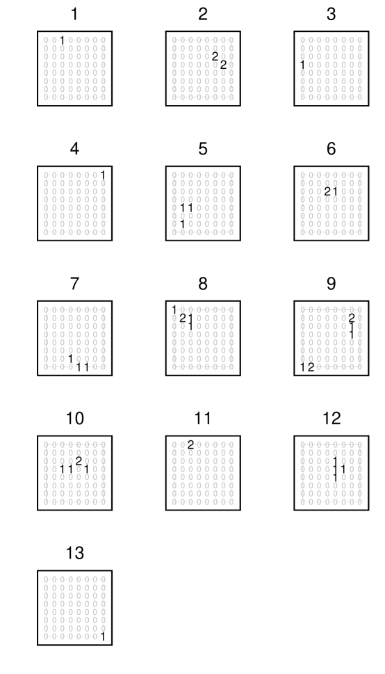
We used a multi-activity center SCR model to simulate the data. This simulation model was based on a superpopulation of individuals, with membership probability which resulted in individuals in our simulated population. We simulated the number of activity centers for each individual from a zero-truncated Poisson distribution with intensity parameter equal to 0.5 and locations of the latent activity centers were sampled as a complete spatial random point process in a square buffered region centered on the unit square study area containing our trap locations for . The buffered region extended units beyond the trap array in each direction to allow the activity centers for some individuals to occur outside the trap array boundary . We used a maximum of the complementary log-log (‘cloglog’) link for the detection function from (2) over all activity centers at each trap location with and . These simulated data resulted in a mixture of unimodal and multimodal space use distributions for the individuals, with individuals observed (Figure 1).
We fit the GCR model as described in the Methods section with priors specified as , , and with support on the set of equally spaced values of . The matrix contains the pairwise distances among traps in our study area and . We set the superpopulation size to individuals for our study area and .
We used the multistage computing strategy to fit the GCR model with MCMC iterations. Stage one required 61.4 minutes and stage two required 1.2 minutes. After fitting the model, post hoc sampling of the abundance required 5.4 minutes and then we used a Gibbs sampler to obtain an MCMC sample for for the simulated individuals 9 and 12. A Gibbs sampler required approximately 36 seconds for each individual. All computation was performed on a machine with a 24-core 3.6 Ghz processor and 192 MB of RAM.
The GCR model fitted to the simulated data resulted in the marginal posterior distributions shown in Figure 2.
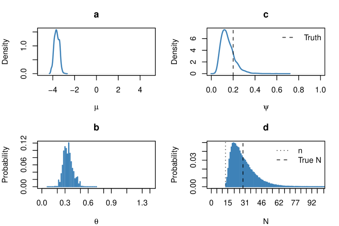
Figure 2a shows a small estimated which implies that the space use throughout most of the study area is low for a given individual. If the species occupied more of the study area, the parameter could increase to accommodate that type of space use.
The marginal posterior mean for population abundance was (compared with the true simulated value ; Figure 2d). The 95% marginal posterior credible interval for abundance was and the marginal posterior quartiles were 21 and 34.
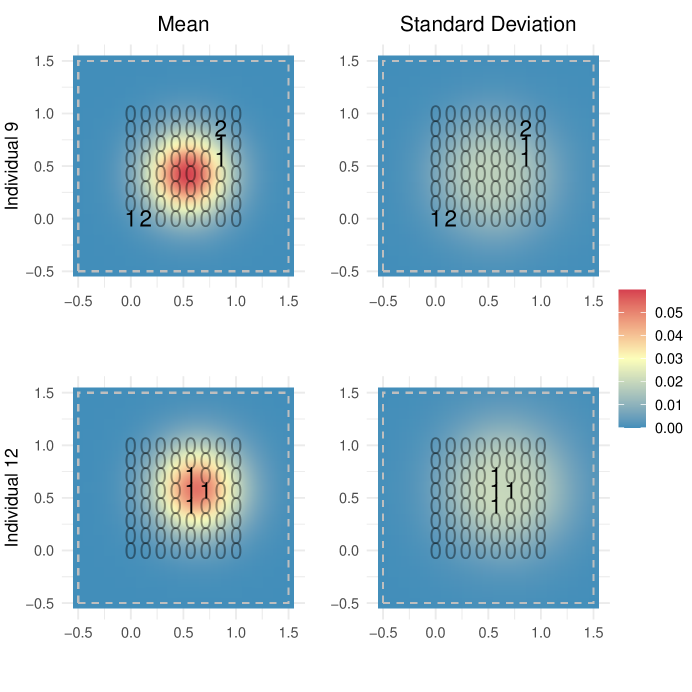
Figure 3 shows the posterior mean (and posterior standard deviation) for the implied space use distribution for two observed individuals in our simulated data; individual 9 illustrates a bimodal space use pattern and individual 12 illustrates a unimodal space use pattern.
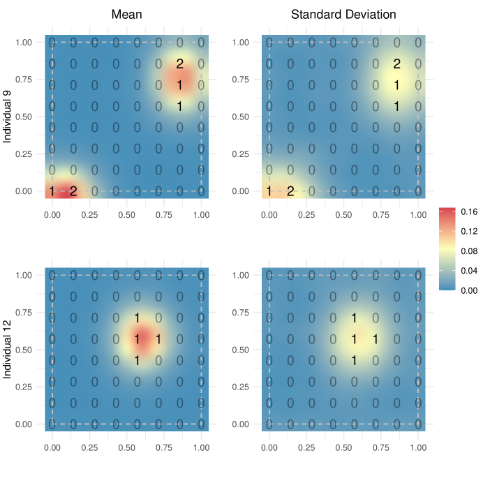
For comparison, we also fit the traditional SCR model with detection function in (1) to the same simulated data (Appendix C), but with the buffer included in the state-space for the latent activity center point process. The results indicate a unimodal symmetric space use pattern between the two sets of detections for individual 9 (Figure 7) rather than the bimodal space use pattern resulting from a fit of the GCR model.
3.2 Snowshoe Hare
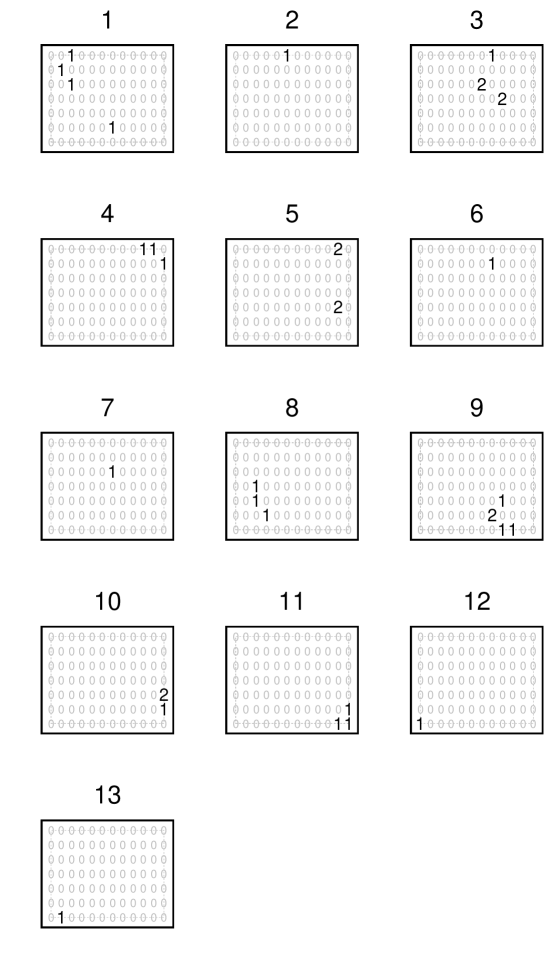
We applied the GCR model to analyze a set of spatially-explicit capture histories of snowshoe hares in Colorado, USA. The data contain counts of detections over sampling occasions at trap locations (Figure 4) and were collected during winter 2007 (Ivan et al., 2014). We defined the study area as the convex hull of the trap locations for this analysis. Exploratory analysis of these data suggest that certain individuals may not use space in a way that meets the assumptions of a standard SCR model because their detections occurred farther apart than those for most other individuals in the study; for example, individuals 1 and 5 in Figure 4.
We fit the GCR model as described in the Methods section with priors specified as , , and with support on the set of equally spaced values, where is the pairwise distance matrix among traps in our study area. We set the superpopulation size to individuals for our study area and to ensure the other parameters were identifiable.
We used MCMC iterations to fit the GCR model. This required 73.3 minutes for stage one, and only 1.4 minutes for stage two of the recursive procedure. To sample the abundance required 7.2 minutes and to sample from the full-conditional for for an individual required approximately 54 seconds using a Gibbs sampler. All computation was performed on a machine with a 24-core 3.6 Ghz processor and 192 MB of RAM.
The GCR model fitted to the snowshoe hare data resulted in marginal posterior distributions shown in Figure 5.
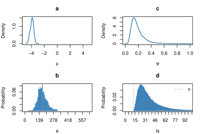
Figure 5 indicates that a small and large were needed to result in adequate smoothness of the space use distribution throughout the study area. Furthermore, the marginal posterior 95% credible interval for abundance was and the marginal posterior quartiles were 24 and 43.
For example, Figure 6 shows the posterior mean (and posterior standard deviation) for the implied space use distribution for two observed individuals in our study that have clearly bimodal space use patterns.
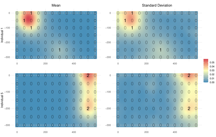
These types of individual-level detection probability patterns (and hence space use patterns) (Figure 6, left column) would not be possible under the conventional SCR model.
4 Discussion
We presented a formulation of spatial capture-recapture models that allows for structured heterogeneity in detection probability over the study area. Our approach assumes the detection probability surface (and hence implied space use distribution) can be characterized by a GP. We refer to this new CR model formulation as “geostatistical” to associate it with the previous studies that have used GPs for modeling other ecological and environmental processes. While there are a variety of approaches to fitting such models to data, we showed how to leverage multicore computing resources based on a multistage computing strategy. By extending the procedure described by Hooten et al. (2023) to accommodate latent GPs, we showed that the GCR model was able to recover total abundance and detection probability patterns that are not unimodal using simulated data.
We also fit the GCR model to capture-recapture data on snowshoe hares in Colorado, USA. Some of the capture histories associated with our observed snowshoe hares showed evidence of multimodality and asymmetric detection probability patterns. The posterior predictive space use distributions we obtained by fitting our GCR model confirmed this.
Whereas conventional SCR models are specified based on an assumption about latent point processes, our approach relies on the flexibility of latent continuous spatial processes. We appreciate the mechanism involved in the conventional SCR model specifications and our GCR model lacks that direct connection to an explicit activity center for each individual. However, we also see the need for additional flexibility in some cases where the space use distributions may not adhere to single elliptical shapes. Furthermore, the latent GP is not without mechanistic connections. For example, in ongoing work, we are exploring the use of multi-output GPs (Alvarez et al., 2012) in GCR models that can account for dependence among individuals explicitly. For example, territorial species may use space that is unoccupied by conspecifics. Therefore we expect those individual space use distributions to be negatively correlated with each other. Our GCR model allows for both negative and positive interactions among individuals to be accounted for using the same types of spatial statistical approaches that have been used to account for dependence among other multivariate spatial processes in nature (e.g., coregionalization and cokriging approaches; Journel and Huijbregts, 1978; Higdon, 2002).
For those interested in multiscale ecological processes, a simpler extension of the GCR approach could facilitate separate inference for individual-based space use and species distribution by allowing for a shared spatially heterogeneous mean function in the latent GP across individuals. That mean function would then represent species distribution due to environmental factors that relate to the fundamental niche. Then the individual-specific spatial random field could account for resource selection and movement at the finer scale.
In fact, a rapidly growing area of development in SCR modeling involves the use of telemetry data (Hooten et al., 2017) coupled with CR data to account for individual-level movement patterns in abundance estimation (e.g., McClintock et al., 2022). Our GCR model could be paired with a telemetry data model in a similar way when both sources of data exist.
Acknowledgments
This research was funded by NSF 1614392 and NSF 2222525. The authors thank the editors and anonymous reviewers of Spatial Statistics as well as Matthias Katzfuss and Antik Chakraborty for helpful discussions and insights about this research.
References
- Albert and Chib (1993) Albert, J. H., and S. Chib. 1993. Bayesian analysis of binary and polychotomous response data. Journal of the American Statistical Association 88:669–679.
- Alvarez et al. (2012) Alvarez, M. A., L. Rosasco, and N. D. Lawrence. 2012. Kernels for vector-valued functions: A review. Foundations and Trends in Machine Learning 4:195–266.
- Borchers and Efford (2008) Borchers, D. L., and M. Efford. 2008. Spatially explicit maximum likelihood methods for capture–recapture studies. Biometrics 64:377–385.
- Chib and Greenberg (1998) Chib, S., and E. Greenberg. 1998. Analysis of multivariate probit models. Biometrika 85:347–361.
- Conn et al. (2018) Conn, P. B., D. S. Johnson, P. J. Williams, S. R. Melin, and M. B. Hooten. 2018. A guide to Bayesian model checking for ecologists. Ecological Monographs 88:526–542.
- de Valpine et al. (2017) de Valpine, P., D. Turek, C. Paciorek, C. Anderson-Bergman, D. Temple Lang, and R. Bodik. 2017. Programming with models: Writing statistical algorithms for general model structures with NIMBLE. Journal of Computational and Graphical Statistics 26:403–413.
- Diggle and Ribeiro Jr (2002) Diggle, P. J., and P. J. Ribeiro Jr. 2002. Bayesian inference in Gaussian model-based geostatistics. Geographical and Environmental Modelling 6:129–146.
- Efford (2019) Efford, M. 2019. Non-circular home ranges and the estimation of population density. Ecology 100:e02580.
- Efford (2011) Efford, M. G. 2011. Estimation of population density by spatially explicit capture–recapture analysis of data from area searches. Ecology 92:2202–2207.
- Efford et al. (2009) Efford, M. G., D. L. Borchers, and A. E. Byrom, 2009. Density estimation by spatially explicit capture–recapture: likelihood-based methods. Pages 255–269 in Modeling Demographic Processes in Marked Populations. Springer.
- Fuller et al. (2016) Fuller, A. K., C. S. Sutherland, J. A. Royle, and M. P. Hare. 2016. Estimating population density and connectivity of American mink using spatial capture–recapture. Ecological Applications 26:1125–1135.
- Higdon (2002) Higdon, D., 2002. Space and space-time modeling using process convolutions. Pages 37–56 in Quantitative methods for current environmental issues. Springer.
- Hooten et al. (2021) Hooten, M. B., D. S. Johnson, and B. M. Brost. 2021. Making recursive Bayesian inference accessible. The American Statistician 75:185–194.
- Hooten et al. (2017) Hooten, M. B., D. S. Johnson, B. T. McClintock, and J. M. Morales. 2017. Animal Movement: Statistical Models for Telemetry Data. CRC press.
- Hooten et al. (2020) Hooten, M. B., X. Lu, M. J. Garlick, and J. A. Powell. 2020. Animal movement models with mechanistic selection functions. Spatial Statistics 37:100406.
- Hooten et al. (2023) Hooten, M. B., M. R. Schwob, D. S. Johnson, and J. S. Ivan. 2023. Multistage hierarchical capture-recapture models. Environmetrics 34:e2799.
- Ivan et al. (2013) Ivan, J. S., G. C. White, and T. M. Shenk. 2013. Using simulation to compare methods for estimating density from capture–recapture data. Ecology 94:817–826.
- Ivan et al. (2014) Ivan, J. S., G. C. White, and T. M. Shenk. 2014. Density and demography of snowshoe hares in central Colorado. The Journal of Wildlife Management 78:580–594.
- Journel and Huijbregts (1978) Journel, A. G., and C. J. Huijbregts. 1978. Mining Geostatistics. Academic Press.
- King et al. (2016) King, R., B. T. McClintock, D. Kidney, and D. Borchers. 2016. Capture–recapture abundance estimation using a semi–complete data likelihood approach. The Annals of Applied Statistics 10:264–285.
- Kordosky et al. (2021) Kordosky, J. R., E. M. Gese, C. M. Thompson, P. A. Terletzky, K. L. Purcell, and J. D. Schneiderman. 2021. Landscape use by fishers (Pekania pennanti): core areas differ in habitat than the entire home range. Canadian Journal of Zoology 99:289–297.
- Lele (2009) Lele, S. R. 2009. A new method for estimation of resource selection probability function. The Journal of Wildlife Management 73:122–127.
- Link (2013) Link, W. A. 2013. A cautionary note on the discrete uniform prior for the binomial N. Ecology 94:2173–2179.
- Lunn et al. (2013) Lunn, D., J. Barrett, M. Sweeting, and S. Thompson. 2013. Fully Bayesian hierarchical modelling in two stages, with application to meta-analysis. Journal of the Royal Statistical Society: Series C (Applied Statistics) 62:551.
- Macqueen and Ruxton (2023) Macqueen, E. I., and G. D. Ruxton. 2023. The adaptive function of construction of multiple non-breeding nests in birds. Ibis 165:1–16.
- McCaslin et al. (2021) McCaslin, H., A. Feuka, and M. Hooten. 2021. Hierarchical computing for hierarchical models in ecology. Methods in Ecology and Evolution 12:245–254.
- McClintock et al. (2022) McClintock, B. T., B. Abrahms, R. B. Chandler, P. B. Conn, S. J. Converse, R. L. Emmet, B. Gardner, N. J. Hostetter, and D. S. Johnson. 2022. An integrated path for spatial capture–recapture and animal movement modeling. Ecology 103:e3473.
- Murray et al. (2010) Murray, I., R. Adams, and D. MacKay, 2010. Elliptical slice sampling. Pages 541–548 in Proceedings of the Thirteenth International Conference on Artificial Intelligence and Statistics. JMLR Workshop and Conference Proceedings.
- Neal (1992) Neal, R. 1992. Bayesian learning via stochastic dynamics. Advances in Neural Information Processing Systems 5:475–482.
- Plummer (2003) Plummer, M., 2003. JAGS: A program for analysis of Bayesian graphical models using Gibbs sampling. Pages 1–10 in Proceedings of the 3rd International Workshop on Distributed Statistical Computing, volume 124. Vienna, Austria.
- Royle (2009) Royle, J. A. 2009. Analysis of capture–recapture models with individual covariates using data augmentation. Biometrics 65:267–274.
- Royle et al. (2013a) Royle, J. A., R. B. Chandler, R. Sollmann, and B. Gardner. 2013a. Spatial Capture-Recapture. Academic Press.
- Royle et al. (2013b) Royle, J. A., R. B. Chandler, C. C. Sun, and A. K. Fuller. 2013b. Integrating resource selection information with spatial capture–recapture. Methods in Ecology and Evolution 4:520–530.
- Royle and Dorazio (2008) Royle, J. A., and R. M. Dorazio. 2008. Hierarchical Modeling and Inference in Ecology: The Analysis of Data from Populations, Metapopulations and Communities. Elsevier.
- Royle and Dorazio (2012) Royle, J. A., and R. M. Dorazio. 2012. Parameter-expanded data augmentation for Bayesian analysis of capture–recapture models. Journal of Ornithology 152:521–537.
- Royle et al. (2018) Royle, J. A., A. K. Fuller, and C. Sutherland. 2018. Unifying population and landscape ecology with spatial capture–recapture. Ecography 41:444–456.
- Royle and Young (2008) Royle, J. A., and K. V. Young. 2008. A hierarchical model for spatial capture–recapture data. Ecology 89:2281–2289.
- Stan Development Team (2023) Stan Development Team, 2023. Stan Modeling Language Users Guide and Reference Manual. URL https://mc-stan.org/.
- Stein (2012) Stein, M. L. 2012. Interpolation of Spatial Data: Some Theory for Kriging. Springer Science & Business Media.
- Sutherland et al. (2015) Sutherland, C., A. K. Fuller, and J. A. Royle. 2015. Modelling non-Euclidean movement and landscape connectivity in highly structured ecological networks. Methods in Ecology and Evolution 6:169–177.
- Sutherland et al. (2019) Sutherland, C., J. A. Royle, and D. W. Linden. 2019. oSCR: A spatial capture–recapture R package for inference about spatial ecological processes. Ecography 42:1459–1469.
- Tourani (2022) Tourani, M. 2022. A review of spatial capture–recapture: Ecological insights, limitations, and prospects. Ecology and Evolution 12:e8468.
- Wilson et al. (2010) Wilson, R. R., M. B. Hooten, B. N. Strobel, and J. A. Shivik. 2010. Accounting for individuals, uncertainty, and multiscale clustering in core area estimation. The Journal of Wildlife Management 74:1343–1352.
- Worton (1989) Worton, B. J. 1989. Kernel methods for estimating the utilization distribution in home-range studies. Ecology 70:164–168.
Appendix A
To show how the form of model that involves conditioning on observed sample size in (5) arises, we demonstrate with a simple capture-recapture (CR) model for brevity in what follows. Extensions to the case where detection probability varies are described in Hooten et al. (2023).
Suppose we have a CR model with modeled as in (1) but with homogeneous detection probability and population membership indicator for . In this case, using PX-DA, for undetected individuals . This results in two sets of data: The original observed data and the augmented zero data . If we marginalize over to yield the “integrated” data model , then we can write the posterior distribution of interest as
| (20) |
where we condition on as an auxiliary source of data because it is unknown until observed as part of the CR survey, like . The first term on the right-hand side in the above expression is irrelevant because the elements of are always known to equal zero when is observed. Thus, the second term in the above expression can be factored as
| (21) |
where the conditional distribution is a zero-truncated binomial and the conditional distribution is either Poisson-binomial or Poisson depending on model assumptions because is the sum of binary variables indicating which individuals in the superpopulation were detected. In our GCR model, the detection probability is heterogeneous and stochastic, thus the conditional distribution for is obtained by marginalizing over .
In terms of implementation of this simple model, for the first stage, we can use an MCMC algorithm with Metropolis-Hastings updates based on a proposal for from its prior (or a random walk). The membership probability can be Monte Carlo sampled directly from its prior because it does not appear in the first-stage conditional data model. In the GCR model, we only have two parameters and . We used a Gaussian random-walk proposal for and a discrete random-walk proposal for and then a block update for both parameters simultaneously.
Appendix B
To sample (and hence ) from its full-conditional distribution after implementing computing stages 1 and 2, we used a Gibbs sampler following a reparameterization of the distribution to include auxiliary variables (Albert and Chib, 1993). This approach was stable and fast relative to sampling using automated software.
As a brief summary of the approach, to sample from the full-conditional distribution of , we recognize that we simply need to use MCMC to fit the model where assuming that and are known (from the stage 2 MCMC output). It is not necessary to sample to fit the broader GCR model because it has been marginalized out in stages 1 and 2, but if we desire inference about the detection probability surface for certain individuals (e.g., Figures 3 and 6), we can obtain a sample for post hoc. We can do this by fitting the model described above while conditioning on each realization of and from the stage 2 output and retain a single realization of (e.g., the last realization in a short chain after burn-in) for each .
For a specific individual and conditional on and , we need only fit a Bayesian binomial generalized linear model (GLM) with probit link function with prior . Thus, the random vector can be treated as a set of parameters in this reduced model. Alternatively, we can write where and is a matrix of spatial basis functions (e.g., we used eigenvectors resulting from the spectral decomposition and is a diagonal matrix of associated eigenvalues). This latter linear model formulation is not strictly necessary but could be used to reduce dimensionality to improve computation time by truncating the matrix and associated dimension of the spectral coefficients . Based on the probit link function and multivariate normal prior for , we can write the model for a given individual of interest as:
| (22) |
where with prior for sampling occasions and is the th row vector of . Jointly for an individual of interest , we can write the model for the latent random vector as
| (23) |
This results in the following tractable full-conditional distributions
| (24) | ||||
| (25) |
where . These full-conditional distributions can be sampled from sequentially in our secondary MCMC algorithm and we obtain the realization as a derived quantity. To predict at a grid of non-trap locations throughout the study area, we sample from its predictive full-conditional distribution (18) as described in the Inference and Prediction section, then transform to and use Monte Carlo integration to obtain posterior moments (i.e., the maps in Figures 3 and 6).
Appendix C
To compare inferred space use patterns, we fit the traditional SCR model from (1) to the simulated data shown in Figure 1 using JAGS. We used the spatial domain from the simulation (extended units beyond the trap array to account for activity center that may fall outside the trap array) and specified vague Gaussian priors for the SCR parameters and , and a uniform prior for . We also used the same superpopulation size .
The GCR model is able to account for irregular detection probability patterns in space, but the SCR model is not. The results of fitting the classical SCR model to our data can be compared with those from the GCR model in terms of the detection probability for a grid of prediction locations.
We note that the predicted detection probability function places the center of probability mass between the two clusters of detections for individual 9 (Figure 7). The radial shape evident in the individual space use patterns is a characteristic of the SCR model and allows it to be powerful when the underlying detection probability meets the assumptions (e.g., for individual 12), but as in this case with simulated individual 9, it may not appropriately represent more complicated patterns (as compared with the GCR results presented in Figure 3). From a model checking perspective (e.g., Conn et al., 2018), we could omit the classical SCR model from our set of candidate models based on these results.