A Nonparametric Mixed-Effects Mixture Model for Patterns of Clinical Measurements Associated with COVID-19

Abstract

Some patients with COVID-19 show changes in signs and symptoms such as temperature and oxygen saturation days before being positively tested for SARS-CoV-2, while others remain asymptomatic. It is important to identify these subgroups and to understand what biological and clinical predictors are related to these subgroups. This information will provide insights into how the immune system may respond differently to infection and can further be used to identify infected individuals. We propose a flexible nonparametric mixed-effects mixture model that identifies risk factors and classifies patients with biological changes. We model the latent probability of biological changes using a logistic regression model and trajectories in the latent groups using smoothing splines. We developed an EM algorithm to maximize the penalized likelihood for estimating all parameters and mean functions. We evaluate our methods by simulations and apply the proposed model to investigate changes in temperature in a cohort of COVID-19-infected hemodialysis patients.

Keywords: clustering, Coronavirus Disease 2019, COVID-19, EM algorithm, mixed-effects model, mixture model, SARS-CoV-2, severe acute respiratory syndrome coronavirus 2, spline

1 Introduction

The Coronavirus Disease 2019 (COVID-19) pandemic has had a profound impact on humanity, and the emergence of new variants of severe acute respiratory syndrome coronavirus 2 (SARS-CoV-2) challenges healthcare systems worldwide. Much research has examined changes in biological variables for diagnosis and prognosis during and after an infection caused by the SARS-CoV-2 (Pimentel et al., 2020; Malik et al., 2021; Chaudhuri et al., 2022). Early detection of SARS-CoV-2 infection based on changes in readily available measurements such as temperature and arterial oxygen saturation during the incubation period is crucial for isolating and treating contagious individuals (de Moraes Batista et al., 2020; Wu et al., 2020; Kukar et al., 2021; Monaghan et al., 2021). Indicators of disease severity and prognosis are essential to the clinical management of COVID-19 patients (Jiang et al., 2020; Malik et al., 2021; Gallo Marin et al., 2021). Identifying potential changes in an individual is challenging because the clinical presentation of COVID-19 varies greatly from asymptomatic infection to critical illness (Harahwa et al., 2020; Souza et al., 2020; da Rosa Mesquita et al., 2021). It is difficult to predict how the disease will manifest itself in an individual. Identifying biological variables, their longitudinal patterns, variations between individuals, and associations with demographic and clinical characteristics would aid the development of a risk-stratified approach to patient care.

Nearly 786,000 people in the United States have an end-stage renal disease (ESRD). About 488,000 ESRD patients travel to clinics to receive life-sustaining hemodialysis (HD) treatments and cannot shelter in place (USRDS, 2020; NIDDK, 2021). HD patients suffer from a host of comorbidities, such as diabetes and cardiac disease, putting them at an increased risk for complications from COVID-19. In addition, HD patients have reduced responses to SARS-CoV-2 vaccines (Simon et al., 2021). Thus, there is a pressing need to identify potential coronavirus carriers and develop procedures to curb the spread among HD patients. Numerous studies (Bivona et al., 2021; Malik et al., 2021; Gallo Marin et al., 2021) focus on the general population but only a few centers on HD patients (Monaghan et al., 2021). The thrice-weekly in-center HD treatments provide results of a large number of clinical and treatment variables that are stored in patients’ electronic health records (EHRs) and thus readily available for analysis. Utilizing EHRs, Chaudhuri et al. (2022) observed significant changes in many biological variables due to COVID-19 infection. However, these results estimated at the population level are not directly applicable to individual detection and prediction. For each patient, we compute temperature change as the difference between measured temperatures minus the average temperatures during a period free of COVID-19 infection. Figure 1 presents temperature change profiles before confirmation time in a cohort of COVID-19 HD patients. Since the body temperature of some patients raised a couple of days before being tested positive for COVID-19, these patterns are indicative of COVID-19 infection. Nevertheless, the temperatures of other patients remain relatively unchanged. We observed similar patterns for other biological variables, including pulse rate, systolic blood pressure, interdialytic weight gain, serum levels of albumin and ferritin, and counts of neutrophils and lymphocytes (Chaudhuri et al., 2022).

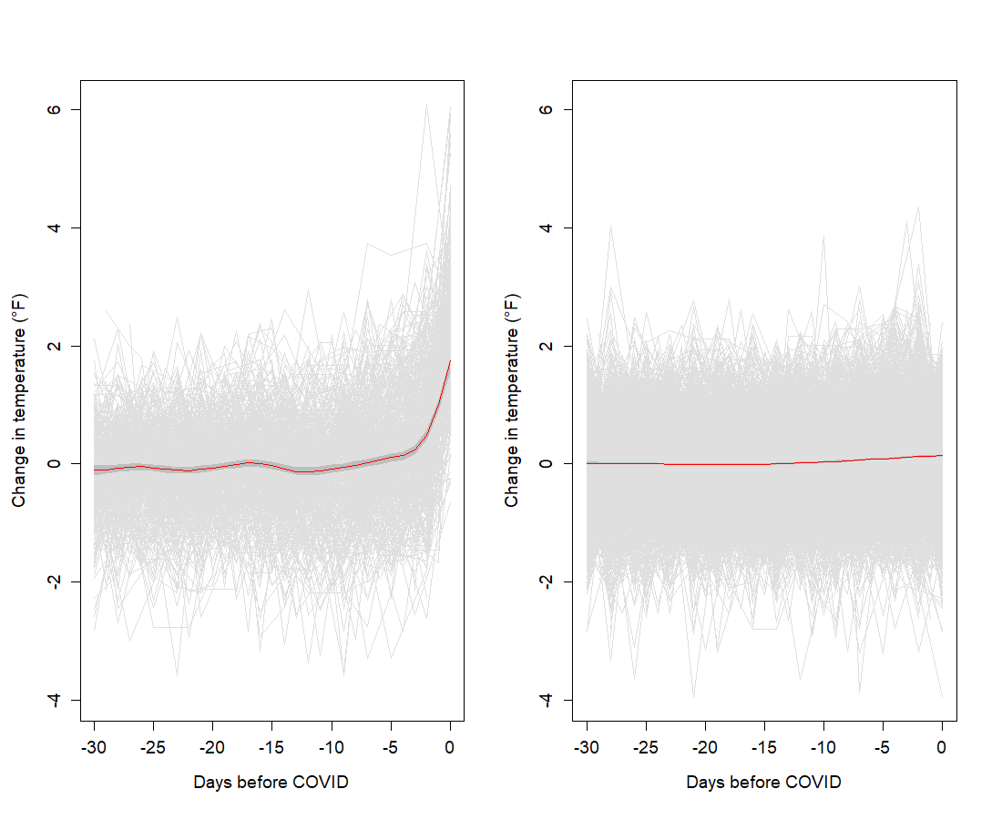
Figure 1: The temperature change profiles before confirmation time in 3,305 COVID-19 HD patients. Red lines are the estimates of mean functions in two groups derived by the method in this paper. Shaded areas are 95% bootstrap confidence intervals.

This paper focuses on estimating changes in biological and clinical indicators in in-center HD patients with COVID-19. We have two objectives: (a) clustering patients into two groups: symptomatic and asymptomatic, and (b) associating the group probability with comorbidities and demographic/clinical characteristics. Existing methods for clustering longitudinal and functional data (see Bouveyron and Brunet (2014) and Jacques and Preda (2014) for reviews) do not apply since they were proposed only for objective (a). We proposed a novel Nonparametric Mixed-Effects Mixture (NMEM) model to fulfill both objectives (a) and (b). We model the probability of a latent group label using a logistic regression model and the response variable when the latent group label is given using a nonparametric mixed-effects model. Joo et al. (2009) considered a similar model with P-spline fixed effects only for the characteristics of urban groundwater recharge. Lu and Song (2012) studied a Bayesian model with B-spline fixed effects and random intercepts for the treatment effect of heroin use. The main contributions of this paper are as follows: (1) modeling both the group mean and subject deviation trajectories using smoothing splines, which makes the proposed NMEM model more flexible than those in Joo et al. (2009) and Lu and Song (2012). Our method extends that in Ma and Zhong (2008) by allowing the probability to depend on covariates; (2) introducing an $L_{1}$ regularization method for variable selection, which Joo et al. (2009) and Lu and Song (2012) did not consider; and (3) investigating changes in temperature in a cohort of COVID-19-infected hemodialysis patients using the proposed method. We note that the proposed method is general, which is not limited to the application illustrated in this paper.

The rest of the paper is organized as follows. We introduce the NMEM model and estimation procedure in Section 2. The real data analysis is reported in Section 3. The simulation and comparisons with other methods are presented in Section 4.

2 Nonparametric Mixed-Effects Mixture Model

2.1 Model Specification

Denote $y_{ij}$ as the observation from subject $i$ at time $t_{ij}$ where $i=1,\ldots,m$ and $j=1,\ldots,n_{i}$. Let $\boldsymbol{y}_{i}=(y_{i1},\ldots,y_{in_{i}})^{T}$ and $\boldsymbol{t}_{i}=(t_{i1},\ldots,t_{in_{i}})^{T}$ be vectors of observations and time points from subject $i$. Let $u_{ik}$ be a latent variable such that $u_{ik}=1$ if subject $i$ belongs to group $k$ and $u_{ik}=0$ otherwise. In this paper, for simplicity, we consider two latent groups (e.g., symptomatic and asymptomatic). The extension to more than two groups is straightforward. Denote $\boldsymbol{x}_{i}$ as a vector of covariates from subject $i$. We assume the following NMEM model:

$$p_{i1} :=P(u_{i1}=1)=\frac{\exp(\beta_{0}+\boldsymbol{x}_{i}^{T}\boldsymbol{\beta}_{1})}{1+\exp(\beta_{0}+\boldsymbol{x}_{i}^{T}\boldsymbol{\beta}_{1})},$$ (1)

$$\boldsymbol{y}_{i} =f_{k}\left(\boldsymbol{t}_{i}\right)+\mathbf{Z}_{i(k)}\mathbf{b}_{i(k)}+\boldsymbol{\epsilon}_{i}\text{ if }u_{ik}=1,\ k=1,2,$$ (2)

where $p_{i1}$ is the probability of subject $i$ belonging to group $1$; $f_{k}(\boldsymbol{t}_{i})=(f_{k}({t}_{i1}),f_{k}({t}_{i2}),...,\\ f_{k}({t}_{in_{1}}))^{T}$ is the mean function in group $k$, $f_{k}$, evaluated at time points $\boldsymbol{t}_{i}$; $\mathbf{Z}_{i(k)}$ is the design matrix for random effects; $\mathbf{b}_{i(k)}\stackrel{{\scriptstyle iid}}{{\sim}}\text{N}(0,\mathbf{G}_{i(k)})$ are the random effects associated with subject $i$ nested within group $k$; $\boldsymbol{\epsilon}_{i}\sim\text{N}(0,\sigma^{2}\mathbf{I}_{n_{i}})$ are the random errors; and $\mathbf{I}_{n_{i}}$ is an identity matrix with dimension $n_{i}$. We assume that $u_{ik}$, $\mathbf{b}_{i(k)}$, and $\boldsymbol{\epsilon}_{i}$ from different subjects are independent.

The logistic regression model in equation (1) models the probability of subject $i$ belonging to group $1$ as a function of covariates, and the nonparametric mixed-effect model in equation (2) models longitudinal trajectories of subject $i$ given the group label. Given a latent group, since the trajectory of the mean function is usually unknown and could be nonlinear, we model the shape of the mean function nonparametrically using a cubic spline. Specifically, we scale time points into the interval $[0,1]$, and assume that $f_{k}\in W_{2}^{2}[0,1]$ where

$$W_{2}^{2}[0,1] =\{f:\ f\text{ and }f^{\prime}\text{ are absolutely continuous},\int_{0}^{1}(f^{\prime\prime}(t))^{2}dt<\infty\}$$

is a Sobolev space. The space can be decomposed into two subspaces $W_{2}^{2}[0,1]=\mathcal{H}_{0}\oplus\mathcal{H}_{1}$, where $\mathcal{H}_{0}=\left\{f:\ f^{\prime\prime}=0\right\}$ and $\mathcal{H}_{1}=\left\{f:\ f(0)=0,\ f^{\prime}(0)=0,\ \int_{0}^{1}\left(f^{\prime\prime}(t)\right)^{2}<\infty\right\}$ are reproducing kernel Hilbert spaces (RKHS) with reproducing kernels (RK) $R_{0}(s,t)=1+k_{1}(s)k_{1}(t)$, $R_{1}(s,t)=k_{2}(s)k_{2}(t)-k_{4}(|s-t|)$, $k_{1}(t)=t-0.5$, $k_{2}(t)=\frac{1}{2}\left(k_{1}^{2}(t)-\frac{1}{12}\right)$, and $k_{4}(t)=\frac{1}{24}\left(k_{1}^{4}(t)-\frac{k_{1}^{2}(t)}{2}+\frac{7}{240}\right)$. See Wang (2011) for details.

The random effects $\mathbf{b}_{i(k)}$ model deviation of subject $i$’s trajectory from the group mean. Different models may be considered for different applications. For example, one may include random intercepts and slopes. Since different subjects may have different nonlinear shapes in our application, we will consider smooth random effects associated with cubic splines (Wang, 1998a). Specifically, in addition to random intercepts and slopes, we will consider a zero mean Gaussian process with covariance function proportional to the RK $R_{1}(s,t)$. Details are given in Section 3.

2.2 Model Estimation

Denote parameters in the covariance matrix of random effects $\mathbf{G}_{i(k)}$ as $\boldsymbol{\zeta}_{k}$. We need to estimate $\beta_{0}$, $\boldsymbol{\beta}_{1}$, $\sigma^{2}$, $f_{1}$, $f_{2}$, $\boldsymbol{\zeta}_{1}$, and $\boldsymbol{\zeta}_{2}$. Denote $N=\sum_{i=1}^{m}n_{i}$ as the total number of observations from all subjects. Let $\boldsymbol{y}=(\boldsymbol{y}_{1}^{T},\ldots,\boldsymbol{y}_{m}^{T})^{T}$, $\boldsymbol{u}_{1}=(u_{11},\ldots,u_{m1})^{T}$, and $\mathbf{V}_{ik}=\mathbf{Z}_{i(k)}\mathbf{G}_{i(k)}\mathbf{Z}_{i(k)}^{T}+\sigma^{2}\mathbf{I}_{n_{i}}$. The complete data likelihood of $(\boldsymbol{y},\boldsymbol{u}_{1})$ is calculated as $p(\boldsymbol{y},\boldsymbol{u}_{1})=p(\boldsymbol{y}|\boldsymbol{u}_{1})p(\boldsymbol{u}_{1})=\prod_{i=1}^{m}p(\boldsymbol{y}_{i}|u_{i1})p(u_{i1})$. We estimate all parameters and nonparametric functions using the following penalized likelihood:

$$l_{c}= \left(\sum_{i=1}^{m}\left[u_{i1}(\beta_{0}+\boldsymbol{x}^{T}_{i}\boldsymbol{\beta}_{1})-\log{(1+\exp{(\beta_{0}+\boldsymbol{x}^{T}_{i}\boldsymbol{\beta}_{1})})}\right]+\lambda_{0}\|\boldsymbol{\beta}_{1}\|\right)$$

$$- \left(\sum_{i=1}^{m}u_{i1}\left[\frac{n_{i}}{2}\log{(2\pi)}+\frac{1}{2}\log{|\mathbf{V}_{i1}|+\frac{1}{2}\left(\boldsymbol{y}_{i}-f_{1}(\boldsymbol{t}_{i})\right)^{T}\mathbf{V}_{i1}^{-1}\left(\boldsymbol{y}_{i}-f_{1}(\boldsymbol{t}_{i})\right)}\right]+N\lambda_{1}\int_{0}^{1}(f_{1}^{\prime\prime})^{2}dt\right)$$

$$- \left(\sum_{i=1}^{m}u_{i2}\left[\frac{n_{i}}{2}\log{(2\pi)}+\frac{1}{2}\log{|\mathbf{V}_{i2}|+\frac{1}{2}\left(\boldsymbol{y}_{i}-f_{2}(\boldsymbol{t}_{i})\right)^{T}\mathbf{V}_{i2}^{-1}\left(\boldsymbol{y}_{i}-f_{2}(\boldsymbol{t}_{i})\right)}\right]+N\lambda_{2}\int_{0}^{1}(f_{2}^{\prime\prime})^{2}dt\right),$$ (3)

where the first part of the first line corresponds to $\log p(\boldsymbol{u}_{1})$, the $L_{1}$ penalty with tuning parameter $\lambda_{0}$ in the second part of the first line is used to select covariates in $\boldsymbol{x}$, the first parts on the second and third lines correspond to $\log p(\boldsymbol{y}|\boldsymbol{u}_{1})$, and the second parts in the second and third lines with smoothing parameters $\lambda_{1}$ and $\lambda_{2}$ control the smoothness of the mean functions in two groups.

Since the latent variables $\boldsymbol{u}_{1}$ are not observed, we use the EM algorithm to estimate the parameters. The E-step of the EM algorithm involves taking the conditional expectation of the likelihood conditional on the data and previously updated parameter values. Denote $\boldsymbol{\theta}=(f_{1},f_{2},\beta_{0},\boldsymbol{\beta}_{1},\boldsymbol{\zeta}_{1},\boldsymbol{\zeta}_{2},\sigma^{2},\lambda_{0},\lambda_{1},\lambda_{2})$ as all the parameters to be estimated in both groups. Note that $u_{ik}$ is Bernoulli. The conditional expectation of the latent variable $u_{ik}$

$$w_{ik}:=P({u_{ik}}=1|\boldsymbol{y}_{i},\hat{\boldsymbol{\theta}})=\frac{P({u_{ik}}=1|\hat{\boldsymbol{\theta}})P(\boldsymbol{y}_{i}|{u_{ik}}=1,\hat{\boldsymbol{\theta}})}{\sum_{k^{\prime}=1}^{2}P(u_{ik^{\prime}}=1|\hat{\boldsymbol{\theta}})P(\boldsymbol{y}_{i}|u_{ik^{\prime}}=1,\hat{\boldsymbol{\theta}})},$$ (4)

where $k\in\{1,2\}$, $\hat{\boldsymbol{\theta}}$ represents the estimated parameters from the last iteration, and $P(\boldsymbol{y}_{i}|u_{ik}=1,\hat{\boldsymbol{\theta}})$ is a multivariate Gaussian density function of $\boldsymbol{y}_{i}$ with mean $f_{k}(\boldsymbol{t}_{i})$ and variance $\mathbf{V}_{ik}$.

The conditional expectation of $l_{c}$ becomes

$$\mathbb{E}(l_{c}\mid\boldsymbol{y},\hat{\boldsymbol{\theta}})=$$

$$\begin{split}&\left(\sum_{i=1}^{m}\left[w_{i1}(\beta_{0}+\boldsymbol{x}^{T}_{i}\boldsymbol{\beta}_{1})-\log{(1+\exp{(\beta_{0}+\boldsymbol{x}^{T}_{i}\boldsymbol{\beta}_{1})})}\right]+\lambda_{0}\|\boldsymbol{\beta}_{1}\|\right)\end{split}$$ (5)

$$\begin{split}-&\left(\sum_{i=1}^{m}w_{i1}\left[\frac{n_{i}}{2}\log{(2\pi)}+\frac{1}{2}\log{|\mathbf{V}_{i1}|+\frac{1}{2}\left(\boldsymbol{y}_{i}-f_{1}(\boldsymbol{t}_{i})\right)^{T}\mathbf{V}_{i1}^{-1}\left(\boldsymbol{y}_{i}-f_{1}(\boldsymbol{t}_{i})\right)}\right]+N\lambda_{1}\int_{0}^{1}(f_{1}^{\prime\prime})^{2}dt\right)\end{split}$$

$$\begin{split}-&\left(\sum_{i=1}^{m}w_{i2}\left[\frac{n_{i}}{2}\log{(2\pi)}+\frac{1}{2}\log{|\mathbf{V}_{i2}|+\frac{1}{2}\left(\boldsymbol{y}_{i}-f_{2}(\boldsymbol{t}_{i})\right)^{T}\mathbf{V}_{i2}^{-1}\left(\boldsymbol{y}_{i}-f_{2}(\boldsymbol{t}_{i})\right)}\right]+N\lambda_{2}\int_{0}^{1}(f_{2}^{\prime\prime})^{2}dt\right)\end{split}$$ (6)

where $w_{i2}=1-w_{i1}$ and $\hat{\boldsymbol{\theta}}$ represents the estimated parameters from the last iteration.

The M-step involves maximizing $E(l_{c}\mid\boldsymbol{y},\hat{\boldsymbol{\theta}})$. We maximize equations (5) and (6) separately since they involve two disjoint set of parameters $\boldsymbol{\theta}_{1}=(\beta_{0},\boldsymbol{\beta}_{1},\lambda_{0})$ and $\boldsymbol{\theta}_{2}=(f_{1},f_{2},\boldsymbol{\zeta}_{1},\boldsymbol{\zeta}_{2},\sigma^{2},\lambda_{1},\lambda_{2})$ respectively.

Equation (5) is the penalized likelihood of a logistic regression model with an $L_{1}$ penalty. We apply the existing method and software package in R (Friedman et al., 2010) to update the estimate of $\boldsymbol{\theta}_{1}$. We use 10-fold cross-validation to select the tuning parameter $\lambda_{0}$.

For equation (6), the mean functions $f_{1}$ and $f_{2}$ are modeled using cubic splines. Based on the decomposition of the Sobolev space $W_{2}^{2}[0,1]=\mathcal{H}_{0}\oplus\mathcal{H}_{1}$, the estimated mean functions can be expressed as (Wang, 2011)

$$f_{k}(t_{ij})=\sum_{\nu=1}^{2}d_{k\nu}\phi_{\nu}(t_{ij})+\sum_{l=1}^{e}c_{kl}\xi_{l}(t_{ij}),\quad k=1,2,$$

where $\phi_{1}(t)=1$ and $\phi_{2}(t)=t$ are basis functions of $\mathcal{H}_{0}$, $\xi_{l}(t)=R_{1}(z_{l},t)$, and $\{z_{1},\cdots,z_{e}\}$ are $e$ distinct points in the set $\{t_{ij},\ i=1,\ldots,m,\ j=1,\ldots,n_{i}\}$. Let $\boldsymbol{d}_{k}=(d_{k1},d_{k2})^{T}$, $\boldsymbol{c}_{k}=(c_{k1},\ldots,c_{ke})^{T}$, and $(\tau_{1},\ldots,\tau_{N})^{T}$ be the stacked vectors of all time points $(t_{11},\ldots,t_{1n_{1}},\ldots,\\ t_{mn_{m}})^{T}$. Denote $\mathbf{S}$ as an $N\times 2$ matrix with the $(\iota,\nu)$th entry $\phi_{\nu}(\tau_{\iota})$, $\mathbf{R}$ as an $N\times e$ matrix with $(\iota,l)$th entry $R_{1}(\tau_{\iota},z_{l})$, and $\mathbf{Q}$ as an $e\times e$ matrix with the $(l,k)$th entry $R_{1}(z_{l},z_{k})$. Let $\mathbf{W}_{k}$ be a block diagonal matrix of size $N\times N$ where the $i$-th block is $w_{ik}\mathbf{V}_{ik}^{-1}$. It is easy to verify that the target equation (6) is proportional to

$$\sum_{i=1}^{m}\left(w_{i1}\log\left|\mathbf{V}_{i1}\right|\right)+\left(\boldsymbol{y}-\mathbf{S}\boldsymbol{d}_{1}-\mathbf{R}\boldsymbol{c}_{1}\right)^{T}\mathbf{W}_{1}\left(\boldsymbol{y}-\mathbf{S}\boldsymbol{d}_{1}-\mathbf{R}\boldsymbol{c}_{1}\right)+N\lambda_{1}\boldsymbol{c}_{1}^{T}\mathbf{Q}\boldsymbol{c}_{1}$$ (7)

$$+ \sum_{i=1}^{m}\left(w_{i2}\log\left|\mathbf{V}_{i2}\right|\right)+\left(\boldsymbol{y}-\mathbf{S}\boldsymbol{d}_{2}-\mathbf{R}\boldsymbol{c}_{2}\right)^{T}\mathbf{W}_{2}\left(\boldsymbol{y}-\mathbf{S}\boldsymbol{d}_{2}-\mathbf{R}\boldsymbol{c}_{2}\right)+N\lambda_{2}\boldsymbol{c}_{2}^{T}\mathbf{Q}\boldsymbol{c}_{2}.$$ (8)

We estimate the variance components $(\sigma^{2},\boldsymbol{\zeta}_{1},\boldsymbol{\zeta}_{2})$ and components corresponding to the mean functions $(\boldsymbol{c}_{1},\boldsymbol{d}_{1},\lambda_{1},\boldsymbol{c}_{2},\boldsymbol{d}_{2},\lambda_{2})$ alternatively.

When fixing the variance components $(\sigma^{2},\boldsymbol{\zeta}_{1},\boldsymbol{\zeta}_{2})$, we estimate the two mean functions and their smoothing parameters in equation (7) and (8) separately. Each one is the penalized least square for smoothing spline regression with correlated data. The minimizer of each satisfies the following equations (Gu, 2013):

$$\left(\begin{array}[]{cc}\mathbf{S}^{T}\mathbf{W}_{k}\mathbf{S}&\mathbf{S}^{T}\mathbf{W}_{k}\mathbf{R}\\ \mathbf{R}^{T}\mathbf{W}_{k}\mathbf{S}&\mathbf{R}^{T}\mathbf{W}_{k}\mathbf{R}+N\lambda_{k}\mathbf{Q}\end{array}\right)\left(\begin{array}[]{l}\boldsymbol{d}_{k}\\ \boldsymbol{c}_{k}\end{array}\right)=\left(\begin{array}[]{c}\mathbf{S}^{T}\mathbf{W}_{k}\boldsymbol{y}\\ \mathbf{R}^{T}\mathbf{W}_{k}\boldsymbol{y}\end{array}\right),\quad k=1,2.$$ (15)

Note that $\mathbf{W}_{k}$ is fixed at this step. Let $w_{ik}\mathbf{V}_{ik}^{-1}=\mathbf{P}_{ik}^{T}\mathbf{P}_{ik}$ be the Cholesky decomposition of $w_{ik}\mathbf{V}_{1k}^{-1}$ and $\mathbf{P}_{k}=\text{diag}(\mathbf{P}_{1k},\cdots,\mathbf{P}_{mk})$. Then $\mathbf{W}_{k}=\mathbf{P}_{k}^{T}\mathbf{P}_{k}$ is the Cholesky decomposition of $\mathbf{W}_{k}=\text{diag}(w_{1k}\mathbf{V}_{1k}^{-1},\cdots,w_{mk}\mathbf{V}_{mk}^{-1})$. With the transformations $\left(\boldsymbol{y}_{k},\mathbf{S}_{k},\mathbf{R}_{k}\right)=\mathbf{P}_{k}^{T}(\boldsymbol{y},\mathbf{S},\mathbf{R})$, the weight matrices $\mathbf{W}_{k}$ in equation (15) are absorbed into other vectors/matrices and the equations reduce to those under the independent cases. Therefore, we can apply computational methods in Gu (2013) for independent data to update $\boldsymbol{c}_{k}$ and $\boldsymbol{d}_{k}$ with smoothing parameters $\lambda_{k}$ selected by the generalized maximum likelihood method.

When fixing the mean functions, we estimate the variance components by minimizing (7) and (8) together using the Limited-memory Broyden–Fletcher–Goldfarb–Shanno (L-BFGS-B) algorithm (Byrd et al., 1995; Zhu et al., 1997). Since both equations contain the common variance of random error $\sigma^{2}$, we profiled it out and minimized the profiled likelihood. We provide the calculation of profiled likelihood in the Appendix.

The initial estimates of variance components and the mean function are calculated using the linear mixed effects (LME) form of smoothing splines. These estimates are then used for the first inner iteration. The existing package nlme can be used for fitting these LME models. Details can be found in Wang (1998b) and Xu and Wang (2021).

We summarize the entire EM algorithm in Algorithm 1. The stopping criteria are set as follows. Let $\boldsymbol{\tilde{\theta}}$ represent all the estimated values except the penalty parameter $\lambda_{0}$ and the smoothing parameters $\lambda_{1}$ and $\lambda_{2}$. Let $d_{EM}^{[\mathcal{O}]}=\frac{\|\boldsymbol{\tilde{\theta}}^{[\mathcal{O}]}-\boldsymbol{\tilde{\theta}}^{[\mathcal{O}-1]}\|^{2}}{\|\boldsymbol{\tilde{\theta}}^{[\mathcal{O}-1]}\|^{2}+\kappa_{1}}$ be the relative change of the estimates at the ${\mathcal{O}}$th EM iteration and $d_{inner}^{[\mathcal{O},\mathcal{I}]}=\frac{\|\boldsymbol{\tilde{\theta}}^{[\mathcal{O},\mathcal{I}]}-\boldsymbol{\tilde{\theta}}^{[\mathcal{O},\mathcal{I}-1]}\|^{2}}{\|\boldsymbol{\tilde{\theta}}^{[\mathcal{O},\mathcal{I}-1]}\|^{2}+\kappa_{2}}$ be the relative change of the estimates at the $\mathcal{I}$th inner iteration inside the ${\mathcal{O}}$th EM iteration. The inner iteration stops if $d_{inner}^{[\mathcal{O},\mathcal{I}]}\leq D_{inner}$ and the EM iteration stops if $d_{EM}^{[\mathcal{O}]}\leq D_{EM}$. The maximum number of iterations are denoted as $\mathcal{O}_{max}$ and $\mathcal{I}_{max}$, respectively.

Input : longitudinal data

Output : estimates of group probabilities, variance components, parameters of covariates and mean functions: $\hat{p}_{ik}$, $\hat{\boldsymbol{\zeta}}_{k}$, $\hat{\sigma}^{2}$, $\hat{\beta_{0}}$, $\hat{\boldsymbol{\beta}_{1}}$, $\hat{f}_{k}$

1 randomly assign subjects with probability 0.5 into two groups where group 1 contains $n_{1}$ subjects and group 2 contains $n_{2}$ subjects;

2 set $\hat{p}_{ik}=n_{k}/N$ for all $i$;

3 get the initial estimates of $\hat{\boldsymbol{\zeta}}_{k},\hat{\sigma}^{2}$ and $\hat{f}_{k}$ using the method introduced in Wang (1998b) and Xu and Wang (2021);

4 while $(\{d_{EM}^{[\mathcal{O}]}>D_{EM}\}\wedge\{\mathcal{O}<=\mathcal{O}_{max}\})$ do

5       E-step:

6       compute $w_{ik}$ as in equation (4) using the current estimates $\hat{p}_{ik}$, $\hat{\boldsymbol{\zeta}}_{k}$, $\hat{\sigma}^{2}$ and $\hat{f}_{k}$;

7       M-step:

8       update $\hat{\boldsymbol{\beta}}$ using logistic regression as in equation (5) and calculate $\hat{p}_{ik}$ as in equation (1);

9       while $(\{d_{inner}^{[\mathcal{O},\mathcal{I}]}>D_{inner}\}\wedge\{\mathcal{I}<=\mathcal{I}_{max}\})$ do

10             solve equation (7) and (8) separately to update $f_{k}$ with fixed $\hat{\boldsymbol{\zeta}}_{k}$ and $\hat{\sigma}^{2}$;

11             minimize the sum of equation (7) and (8) to update $\hat{\boldsymbol{\zeta}}_{k}$ and $\hat{\sigma}^{2}$ with fixed $f_{k}$ using L-BFGS-B;

12            

13       end while

14      

15 end while

return $\hat{p}_{ik}$, $\hat{\boldsymbol{\zeta}}_{k}$, $\hat{\sigma}^{2}$, $\hat{\beta_{0}}$, $\hat{\boldsymbol{\beta}_{1}}$, $\hat{f}_{k}$

Algorithm 1 EM algorithm for fitting the NMEM model

We regard the $L_{1}$ penalty in the logistic regression as a variable selection process. After variable selection, we rerun Algorithm 1 without the $L_{1}$ penalty and get the point estimate of all parameters.

We construct bootstrap confidence intervals for the estimated mean functions and all parameters.

3 Temperature Profiles in COVID-19-Infected HD Patients

This section applies our methods to investigate temperature change profiles before COVID-19 confirmation in HD patients. We consider 3,305 ESRD patients who received in-center HD treatment from Fresenius Medical Care and had positive PCR tests during 2020-01-01 and 2021-8-31. We align patients at their first positive PCR test date and analyze their temperature measurements 30 days before the PCR test. The observation window is defined as -30 to 0, where 0 is the PCR test date. To focus on the changing pattern, we subtract each patient’s temperature from the average temperature between -60 to -31 days, a period free of COVID-19 infection. Figure 1 shows temperature change profiles for all patients. Our goals are to identify two latent groups (symptomatic and asymptomatic), estimate the probability of belonging to each group for each subject, and associate the group probability with demographic and clinical characteristics.

Based on preliminary analyses, we consider an NMEM model with equation (1) and the following model in replace of equation (2):

$$\boldsymbol{y}_{i} =f_{k}\left(\boldsymbol{t}_{i}\right)+b_{i1(k)}\mathbf{1}+b_{i2(k)}\boldsymbol{t}_{i}+s_{i(k)}\left(\boldsymbol{t}_{i}\right)+\boldsymbol{\epsilon}_{i},\text{ if $u_{ik}=1$, }k=1,2,$$ (16)

where groups $1$ and $2$ correspond to patients with and without temperature changes, $f_{1}$ and $f_{2}$ are the mean functions of these two groups, $b_{i1(k)}$, $b_{i2(k)}$, and $s_{i(k)}(\boldsymbol{t}_{i})=(s_{i(k)}(t_{i,1}),\cdots,s_{i(k)}(t_{i,n_{i}}))^{T}$ are random intercept, slope, and a vector of smooth random effects associated with subject $i$ nested within group $k$, and $\boldsymbol{\epsilon}_{i}\sim\text{N}(0,\sigma^{2}\boldsymbol{I}_{n_{i}})$ are random errors independent of the random effects. Model (16) is a special case of the proposed model (2) with $\mathbf{Z}_{i(k)}=(\boldsymbol{1},\boldsymbol{t}_{i},\mathbf{I}_{n_{i}})$ and $\boldsymbol{b}_{i(k)}=(b_{i1(k)},b_{i2(k)},s_{i(k)}(t_{i,1}),\cdots,s_{i(k)}(t_{i,n_{i}}))^{T}$. We assume unstructured covariance for the random intercept and slope. In addition to the random intercept and slope, the smooth random effect $s_{i(k)}(t)$ is a function of $t$ that allows a more flexible deviation of subject $i$ from the population mean (Wang, 2011). We assume that $s_{i(k)}(t)$ follows a zero mean Gaussian process with the covariance function equals the reproducing kernel of $\mathcal{H}_{1}$. Specifically, for the combined random effects, we assume that

$$\boldsymbol{b}_{i(k)} =\left(\begin{array}[]{c}b_{i1(k)}\\ b_{i2(k)}\\ \hline\cr s_{i(k)}(t_{i,1})\\ \vdots\\ s_{i(k)}(t_{i,n_{i}})\end{array}\right)\sim\text{N}\left(\boldsymbol{0},\left[\begin{array}[]{c|c}\begin{array}[]{cc}\sigma^{2}_{inter,k}&\sigma_{is,k}\\ \sigma_{is,k}&\sigma^{2}_{slope,k}\\ \end{array}&\mathbf{0}\\ \hline\cr\mathbf{0}&\begin{array}[]{cc}\sigma^{2}_{non,k}R_{1}(\boldsymbol{t}_{i},\boldsymbol{t}_{i})\end{array}\end{array}\right]\right),$$ (27)

for $k\in\{1,2\}$, where $\sigma^{2}_{inter,k}$, $\sigma^{2}_{slope,k}$, and $\sigma_{is,k}$ are variances and covariance of the random intercept and slope, $\sigma^{2}_{non,k}$ is the variance of smooth random effect, and $R_{1}(\boldsymbol{t}_{i},\boldsymbol{t}_{i})$ is an $n_{i}\times n_{i}$ matrix with the $jk$th entry as $R_{1}(t_{ij},t_{ik})$. For model (16), we have $\boldsymbol{\zeta}_{k}=(\sigma^{2}_{inter,k},\sigma_{is,k},\sigma^{2}_{slope,k},\sigma^{2}_{non,k})$, $k\in\{1,2\}$.

Based on exploratory analysis and literature, we consider the following covariates for the logistic regression model (1): gender, race, ethnicity, vintage, diabetes, hypertension, BMI (calculated using height and the average weight after each dialysis treatment during the observation window), age on the treatment date, and vascular access type with three options: arteriovenous fistula (AVF), arteriovenous grafts (AVG), and central venous catheter (CVCATH).

For the stopping criteria, we set $\kappa_{1}=\kappa_{2}=10^{-5}$, $D_{EM}=10^{-5}$, $D_{inner}=10^{-5}$, $\mathcal{O}_{max}=100$, and $\mathcal{I}_{max}=5$. After variable selection, we refit the model with selected variables and without the $L_{1}$ penalty. To avoid over-fitting, we set a lower bound for $\lambda_{k}$ as $\log_{10}(N\lambda_{k})=0$ where $N=47013$. The variance components in equation (27) are estimated using the covariance matrix of bivariate normal where $\sigma_{is,1}=\rho\sigma_{inter,1}\sigma_{slope,1}$. All variances are estimated using natural log transformation, and a tangent transformation is used for the correlation parameter $\rho$.

We summarize estimates of coefficients associated with covariates, variance components, and their 95% bootstrap confidence intervals based on $1000$ sampled from the fitted model in Table 1.

We conclude that white and elderly patients were less likely to have a change in temperature. Age can reflect the strength of the patient’s immune system. Elderly patients usually have a weaker immune system and are thus less responsive to the infection.

Table 1: Result of data analysis. Upper: estimates of variance components. Lower: estimates of coefficients in the logistic regression model. We only report the variables selected by Lasso. We report the point estimate and 95% confidence intervals. The subscripts for variance components are defined in equation (27). The subscripts for covariates with a “Y" indicate the patient has that comorbidity.

Parameters	Estimate	95% CI
$\hat{\sigma}^{2}$	0.4142	(0.4096,0.4184)
$\hat{\sigma}_{inter,1}^{2}$	0.0958	(0.0714,0.1209)
$\hat{\sigma}_{inter,2}^{2}$	0.0625	(0.0547,0.0710)
$\hat{\sigma}_{is,1}$	-0.0817	(-0.1208,-0.0418)
$\hat{\sigma}_{is,2}$	-0.0147	(-0.0245,-0.0052)
$\hat{\sigma}_{slope,1}$	0.5125	(0.4060,0.6040)
$\hat{\sigma}_{slope,2}$	0.0980	(0.0763,0.1160)
$\hat{\sigma}_{non,1}^{2}$	14.5024	(11.1972,17.1201)
$\hat{\sigma}_{non,2}^{2}$	0.2192	(0.0000,0.6954)
$\hat{\beta}_{0}$	-1.1048	(-1.7839,-0.2815)
$\hat{\beta}_{Male}$	0.0870	(-0.1346,0.3090)
$\hat{\beta}_{White}$	-0.3788	(-0.6232,-0.1346)
$\hat{\beta}_{DiabetesY}$	-0.1131	(-0.3531,0.1177)
$\hat{\beta}_{BMI}$	0.0147	(-0.0001,0.0283)
$\hat{\beta}_{age}$	-0.0103	(-0.0182,-0.0013)
$\hat{\beta}_{AVG}$	0.2056	(-0.1235,0.5117)
$\hat{\beta}_{CVCATH}$	-0.1593	(-0.4913,0.1268)

With the probability threshold for clustering set as $0.5$, our method identified 470 (14.22%) out of 3,305 COVID-19 patients who experienced an increase in temperature before the positive PCR test. Figure 2 shows the estimated mean change functions and their 95% confidence intervals in the two groups. We note that confidence intervals for the mean functions are narrow due to a large number of total observations. As we can see, in group 1, the increase in temperature started about nine days and accelerated about four days before the PCR test date.

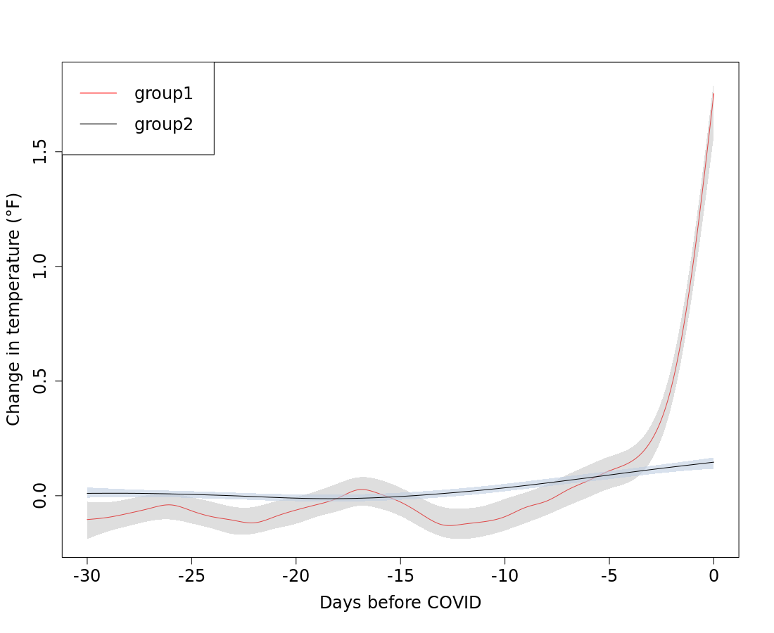
Figure 2: Estimated mean functions of two groups and their 95% bootstrap confidence intervals.

4 Simulation Study

We conduct simulations to evaluate the performance of the proposed method and compare it with the previous work in Lu and Song (2012). Lu and Song (2012) considered the following model:

$$P(u_{ik}=1)=p_{ik}=\frac{\exp(\beta_{0}+\boldsymbol{x}_{i}^{T}\boldsymbol{\beta}_{k})}{\sum_{k^{\prime}=1}^{2}\exp(\beta_{0}+\boldsymbol{x}_{i}^{T}\boldsymbol{\beta}_{k^{\prime}})},\quad i=1,\ldots,m,$$

$$\boldsymbol{y}_{i}=\tilde{\mathbf{X}}^{[1]}_{i}f_{k}(\mathbf{t}_{i})+\tilde{\mathbf{X}}^{[2]}_{i}\boldsymbol{\alpha}_{k}+\mathbf{Z}_{i(k)}\mathbf{b}_{i(k)}+\boldsymbol{\epsilon}_{ik}\quad\text{ if }u_{ik}=1,$$ (28)

where $\tilde{\mathbf{X}}^{[1]}_{i}$ and $\tilde{\mathbf{X}}^{[2]}_{i}$ are the design matrices of fixed effects $f_{k}(\mathbf{t}_{i})$ and $\boldsymbol{\alpha}_{k}$ respectively, $\mathbf{Z}_{i(k)}$ is the design matrix for the random effects $\mathbf{b}_{i(k)}$, and the variances of random errors $\boldsymbol{\epsilon}_{ik}$ are assumed to be different for different groups.

Our method differs from Lu and Song’s methods in both the model structure and estimation approach. Lu and Song (2012) modeled the nonparametric functions $f_{k}$’s using P-splines while we use smoothing splines. Our proposed model includes a smooth random effect for flexibility and allows different random effects in different groups. Lu and Song (2012) estimate parameters in a Bayesian framework while we estimate parameters using penalized likelihood. In addition, our estimation procedure includes an $L_{1}$ penalty for variable selection.

We generate data using model (1) and (16), which was used in real data analysis in Section 3. We set $m=3305$ and set parameters as their estimates when possible.

We generate latent variables $u_{i1}$ for $i=1,\cdots,m$ using equation (1). We include all nine covariates (before variable selection) for the group probability in equation (1) and generated them according to their estimated marginal distributions. Specifically, six categorical variables are generated according to their empirical ratios in each category. Three continuous variables are generated from an exponential distribution with a rate parameter of $0.22$ (vintage), a Gamma distribution with a shape parameter of $15.5$ and a rate parameter of $0.5$ (BMI), and a normal distribution with a mean $62$ and standard deviation $14$ (age). Parameters in three continuous distributions are set to be the maximum likelihood estimates. For the $\boldsymbol{\beta}$ coefficients in the logistic model (1), we set the intercept as the estimate in Table 1, coefficients for gender, ethnicity, vintage, diabetes, hypertension, BMI, and vascular access types as zero since they are either not selected in the variable selection process or the confidence interval contains zero in the final estimation. The coefficients for race and age are set to be the estimates in Table 1. The latent variables $u_{i1}$ for $i=1,\cdots,m$ are generated according to a Bernoulli distribution with probability given in equation (1).

We use equation (16) to generate responses $\boldsymbol{y}_{i}$. Since Lu and Song (2012)’s model does not have a smooth random effect, we consider two simulation settings: with smooth random effect where $\sigma_{non,1}^{2}=14.5$ (estimate from the real data), $\sigma_{non,2}^{2}=14$ and without smooth random effect where $\sigma_{non,1}^{2}=\sigma_{non,2}^{2}=0$. In both settings, the values of all other parameters apart from the variance of smooth random effect are set to be the estimates in the real data analysis in Table 1. We first randomly generate the number of observations $n_{i}$ from a discrete uniform distribution on $[16,31]$ for each subject $i$, and then randomly select $n_{i}$ days between -30 to 0 as $\boldsymbol{t}_{i}$. The values of mean functions $f_{k}$ at each time point are set to be the estimates in the real data analysis. Independent and identically distributed random errors are generated from a normal distribution with mean zero and variance equals the estimate from the real data analysis.

To fit model (28), we set $\tilde{\mathbf{X}}^{[1]}_{i}$ as an identity matrix and $\tilde{\mathbf{X}}^{[2]}_{i}=0$. Lu and Song (2012) used the random permutation sampler approach in Frühwirth-Schnatter (2001) to deal with the label-switching problem caused by the symmetric prior of the parameters in different components. We use the variance of random slope for the permutation sampler in our simulations.

Each simulation is replicated $100$ times. We use the same stopping criteria as in the real data analysis. The comparison results are presented in Table 2, Figure 3 and Figure 4.

Both methods performed well when no smooth random effect existed. The clustering accuracy and MSEs of function estimates are almost identical. The existence of a smooth random effect allows nonlinear individual departure from the population mean function, thus making clustering and estimation more difficult. This is reflected in the smaller accuracy and larger MSEs in Table 2. As expected, our method achieves better accuracy and lower MSEs than Lu and Song’s method when smooth random effect existed. In general, our method has smaller biases in the estimates of variance components (Figures 3 and 4).

Table 2: Simulation results: average accuracy in the two settings. NMEM stands for our method, LS stands for LU and Song’s method. We also report the average mean squared error (MSE) of estimated mean functions.

3	Without $\sigma^{2}_{non,k}$		With $\sigma^{2}_{non,k}$
	NMEM	LS	NMEM	LS
2 Accuracy	0.9368	0.9367	0.8115	0.6251
MSE $f_{1}$	0.0017	0.0019	0.0280	0.0513
MSE $f_{2}$	0.0001	0.0001	0.0007	0.0165
3

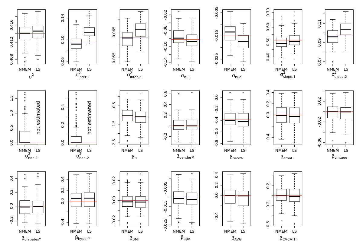
Figure 3: Simulation results without smooth random effects: box plots of estimated parameters from NMEM and Lu and Song’s method (LS). Red lines are true values of parameters.

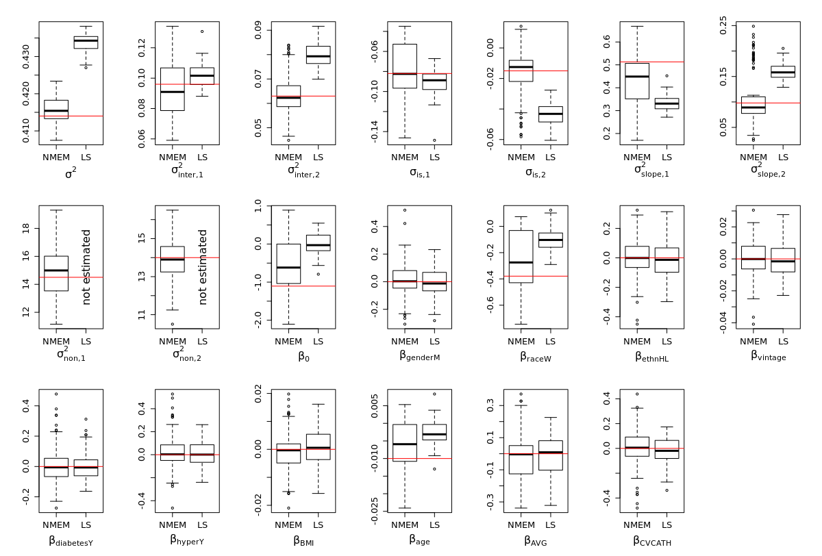
Figure 4: Simulation results with smooth random effects: box plots of estimated parameters from NMEM and Lu and Song’s method (LS). Red lines are true values of parameters.

We also conducted a simulation study to test the performance of variable selection. The values of all parameters, including the variance of the smooth random effects, are set to be the estimates in the real data analysis in table 1. For variable selection in the model (1), on average, $0.3$ of the two non-zero parameters (not including the intercept) are mistakenly excluded from the model, and $2.87$ out of the eight zero parameters are mistakenly selected. The over-selection behavior agrees with the previous literature (Tibshirani, 1996; Chetverikov et al., 2021).

5 Conclusion

This article proposes a unified method for clustering longitudinal trajectories and relating the subgroups to other biological and clinical predictors. A flexible nonparametric mixed-effects mixture model is proposed to identify risk factors and classify patients with a change in body temperature before the diagnosis of COVID-19. We model the change in temperature using smoothing splines. We use penalized likelihood and the EM algorithm to estimate the mean functions, variance components, and covariates associated with the clustering probability. A simulation study shows that our method performs well and, under certain scenarios, outperforms existing methods. The results of data analysis suggest that different demographic characteristics influence the immune system response and provide an improved understanding of patient groups that may or may not experience a more severe course following infection with SARS-CoV-2.

Appendix A Profiled Likelihood

Recall equation (7) and (8) in the paper,

$$\sum_{i=1}^{m}\left(w_{i1}\log\left|\mathbf{V}_{i1}\right|\right)+\left(\boldsymbol{y}-\mathbf{S}\boldsymbol{d}_{1}-\mathbf{R}\boldsymbol{c}_{1}\right)^{T}\mathbf{W}_{1}\left(\boldsymbol{y}-\mathbf{S}\boldsymbol{d}_{1}-\mathbf{R}\boldsymbol{c}_{1}\right)+N\lambda_{1}\boldsymbol{c}_{1}^{T}\mathbf{Q}\boldsymbol{c}_{1}$$ (29)

$$+ \sum_{i=1}^{m}\left(w_{i2}\log\left|\mathbf{V}_{i2}\right|\right)+\left(\boldsymbol{y}-\mathbf{S}\boldsymbol{d}_{2}-\mathbf{R}\boldsymbol{c}_{2}\right)^{T}\mathbf{W}_{2}\left(\boldsymbol{y}-\mathbf{S}\boldsymbol{d}_{2}-\mathbf{R}\boldsymbol{c}_{2}\right)+N\lambda_{2}\boldsymbol{c}_{2}^{T}\mathbf{Q}\boldsymbol{c}_{2}.$$ (30)

We can rewrite equations (29) and (30) as

$$\begin{split}&\sum_{i=1}^{m}\Big{[}w_{i1}\log{|\mathbf{V}_{i1}|}+w_{i2}\log{|\mathbf{V}_{i2}|}+w_{i1}(\boldsymbol{y}_{i}-\mathbf{S}_{i}\boldsymbol{d}_{1}-\mathbf{R}_{i}\boldsymbol{c}_{1})^{T}\mathbf{V}_{i1}^{-1}(\boldsymbol{y}_{i}-\mathbf{S}_{i}\boldsymbol{d}_{1}-\mathbf{R}_{i}\boldsymbol{c}_{1})\\ &+w_{i2}(\boldsymbol{y}_{i}-\mathbf{S}_{i}\boldsymbol{d}_{2}-\mathbf{R}_{i}\boldsymbol{c}_{2})^{T}\mathbf{V}_{i2}^{-1}(\boldsymbol{y}_{i}-\mathbf{S}_{i}\boldsymbol{d}_{2}-\mathbf{R}_{i}\boldsymbol{c}_{2})\Big{]}\end{split}$$

$$\begin{split}=&\sum_{i=1}^{m}\Big{[}n_{i}\log{\sigma^{2}}+w_{i1}\log{|\mathbf{V}_{i1}^{*}|}+w_{i2}\log{|\mathbf{V}_{i2}^{*}|}\\ &+\frac{w_{i1}}{\sigma^{2}}(\boldsymbol{y}_{i}-\mathbf{S}_{i}\boldsymbol{d}_{1}-\mathbf{R}_{i}\boldsymbol{c}_{1})^{T}\mathbf{V}_{i1}^{*-1}(\boldsymbol{y}_{i}-\mathbf{S}_{i}\boldsymbol{d}_{1}-\mathbf{R}_{i}\boldsymbol{c}_{1})\\ &+\frac{w_{i2}}{\sigma^{2}}(\boldsymbol{y}_{i}-\mathbf{S}_{i}\boldsymbol{d}_{2}-\mathbf{R}_{i}\boldsymbol{c}_{2})^{T}\mathbf{V}_{i2}^{*-1}(\boldsymbol{y}_{i}-\mathbf{S}_{i}\boldsymbol{d}_{2}-\mathbf{R}_{i}\boldsymbol{c}_{2})\Big{]},\end{split}$$

where $\mathbf{V}_{i1}^{*}=\mathbf{V}_{i1}/\sigma^{2}$ and $\mathbf{V}_{i2}^{*}=\mathbf{V}_{i2}/\sigma^{2}$.

Therefore we have,

$$\begin{split}\hat{\sigma}^{2}=\frac{1}{N}\sum_{i=1}^{m}\Big{[}&w_{i1}(\boldsymbol{y}_{i}-\mathbf{S}_{i}\boldsymbol{d}_{1}-\mathbf{R}_{i}\boldsymbol{c}_{1})^{T}\mathbf{V}_{i1}^{*-1}(\boldsymbol{y}_{i}-\mathbf{S}_{i}\boldsymbol{d}_{1}-\mathbf{R}_{i}\boldsymbol{c}_{1})+\\ &w_{i2}(\boldsymbol{y}_{i}-\mathbf{S}_{i}\boldsymbol{d}_{2}-\mathbf{R}_{i}\boldsymbol{c}_{2})^{T}\mathbf{V}_{i2}^{*-1}(\boldsymbol{y}_{i}-\mathbf{S}_{i}\boldsymbol{d}_{2}-\mathbf{R}_{i}\boldsymbol{c}_{2})\Big{]}.\end{split}$$

Plugging the above back we get the profiled likelihood:

$$l_{p}=N\log\Big{(}\sum_{i=1}^{m}\Big{[} w_{i1}\left(\boldsymbol{y}_{i}-\mathbf{S}_{i}\boldsymbol{d}_{1}-\mathbf{R}_{i}\boldsymbol{c}_{1}\right)^{T}\mathbf{V}_{i1}^{*-1}\left(\boldsymbol{y}_{i}-\mathbf{S}_{i}\boldsymbol{d}_{1}-\mathbf{R}_{i}\boldsymbol{c}_{1}\right)+$$

$$w_{i2}\left(\boldsymbol{y}_{i}-\mathbf{S}_{i}\boldsymbol{d}_{2}-\mathbf{R}_{i}\boldsymbol{c}_{2}\right)^{T}\mathbf{V}_{i2}^{*-1}\left(\boldsymbol{y}_{i}-\mathbf{S}_{i}\boldsymbol{d}_{2}-\mathbf{R}_{i}\boldsymbol{c}_{2}\right)\Big{]}\Big{)}$$

$$+\sum_{i=1}^{m}\Big{[}w_{i1}\log\left|\mathbf{V}_{i1}^{*}\right|+w_{i2}\log\left|\mathbf{V}_{i2}^{*}\right|\Big{]}.$$

Appendix B funding

This research is partially supported by NIH grants R01-DK130067, R01-HL161303, R01-DK117208, and NSF grant DMS-2053423.

References

- Pimentel et al. [2020] Marco A.F. Pimentel, Oliver C. Redfern, Robert Hatch, J. Duncan Young, Lionel Tarassenko, and Peter J. Watkinson. Trajectories of vital signs in patients with covid-19. Resuscitation, 156:99–106, 2020. ISSN 0300-9572. doi:https://doi.org/10.1016/j.resuscitation.2020.09.002. URL https://www.sciencedirect.com/science/article/pii/S0300957220304408.
- Malik et al. [2021] Preeti Malik, Urvish Patel, Deep Mehta, Nidhi Patel, Raveena Kelkar, Muhammad Akrmah, Janice L Gabrilove, and Henry Sacks. Biomarkers and outcomes of COVID-19 hospitalisations: systematic review and meta-analysis. BMJ Evidence-Based Medicine, 26(3):107–108, 6 2021. ISSN 2515-446X, 2515-4478. doi:10.1136/bmjebm-2020-111536. URL https://ebm.bmj.com/lookup/doi/10.1136/bmjebm-2020-111536.
- Chaudhuri et al. [2022] Sheetal Chaudhuri, Rachel Lasky, Yue Jiao, John Larkin, Caitlin Monaghan, Anke Winter, Luca Neri, Peter Kotanko, Jeffrey Hymes, Sangho Lee, Yuedong Wang, Jeroen P. Kooman, Franklin Maddux, and Len Usvyat. Trajectories of clinical and laboratory characteristics associated with covid-19 in hemodialysis patients by survival. Hemodialysis International, 26(1):94–107, 1 2022. ISSN 1492-7535, 1542-4758. doi:10.1111/hdi.12977. URL https://onlinelibrary.wiley.com/doi/10.1111/hdi.12977.
- de Moraes Batista et al. [2020] André Filipe de Moraes Batista, João Luiz Miraglia, Thiago Henrique Rizzi Donato, and Alexandre Dias Porto Chiavegatto Filho. COVID-19 diagnosis prediction in emergency care patients: a machine learning approach. preprint, Epidemiology, 4 2020. URL http://medrxiv.org/lookup/doi/10.1101/2020.04.04.20052092.
- Wu et al. [2020] Jiangpeng Wu, Pengyi Zhang, Liting Zhang, Wenbo Meng, Junfeng Li, Chongxiang Tong, Yonghong Li, Jing Cai, Zengwei Yang, Jinhong Zhu, Meie Zhao, Huirong Huang, Xiaodong Xie, and Shuyan Li. Rapid and accurate identification of COVID-19 infection through machine learning based on clinical available blood test results. preprint, Infectious Diseases (except HIV/AIDS), 4 2020. URL http://medrxiv.org/lookup/doi/10.1101/2020.04.02.20051136.
- Kukar et al. [2021] Matjaž Kukar, Gregor Gunčar, Tomaž Vovko, Simon Podnar, Peter Černelč, Miran Brvar, Mateja Zalaznik, Mateja Notar, Sašo Moškon, and Marko Notar. COVID-19 diagnosis by routine blood tests using machine learning. Scientific Reports, 11(1):10738, 12 2021. ISSN 2045-2322. doi:10.1038/s41598-021-90265-9. URL http://www.nature.com/articles/s41598-021-90265-9.
- Monaghan et al. [2021] Caitlin K. Monaghan, John W. Larkin, Sheetal Chaudhuri, Hao Han, Yue Jiao, Kristine M. Bermudez, Eric D. Weinhandl, Ines A. Dahne-Steuber, Kathleen Belmonte, Luca Neri, Peter Kotanko, Jeroen P. Kooman, Jeffrey L. Hymes, Robert J. Kossmann, Len A. Usvyat, and Franklin W. Maddux. Machine Learning for Prediction of Patients on Hemodialysis with an Undetected SARS-CoV-2 Infection. Kidney360, 2(3):456–468, 3 2021. ISSN 2641-7650. doi:10.34067/KID.0003802020. URL https://kidney360.asnjournals.org/lookup/doi/10.34067/KID.0003802020.
- Jiang et al. [2020] Xiangao Jiang, Megan Coffee, Anasse Bari, Junzhang Wang, Xinyue Jiang, Jianping Huang, Jichan Shi, Jianyi Dai, Jing Cai, Tianxiao Zhang, Zhengxing Wu, Guiqing He, and Yitong Huang. Towards an Artificial Intelligence Framework for Data-Driven Prediction of Coronavirus Clinical Severity. Computers, Materials & Continua, 62(3):537–551, 2020. ISSN 1546-2226. doi:10.32604/cmc.2020.010691. URL https://www.techscience.com/cmc/v63n1/38464.
- Gallo Marin et al. [2021] Benjamin Gallo Marin, Ghazal Aghagoli, Katya Lavine, Lanbo Yang, Emily J. Siff, Silvia S. Chiang, Thais P. Salazar-Mather, Luba Dumenco, Michael C Savaria, Su N. Aung, Timothy Flanigan, and Ian C. Michelow. Predictors of COVID-19 severity: A literature review. Reviews in Medical Virology, 31(1):1–10, 1 2021. ISSN 1052-9276, 1099-1654. doi:10.1002/rmv.2146. URL https://onlinelibrary.wiley.com/doi/10.1002/rmv.2146.
- Harahwa et al. [2020] Tinotenda A. Harahwa, Thomas Ho Lai Yau, Mae-Sing Lim-Cooke, Salah Al-Haddi, Mohamed Zeinah, and Amer Harky. The optimal diagnostic methods for COVID-19. Diagnosis, 7(4):349–356, 11 2020. ISSN 2194-802X, 2194-8011. doi:10.1515/dx-2020-0058. URL https://www.degruyter.com/document/doi/10.1515/dx-2020-0058/html.
- Souza et al. [2020] Tiago H. Souza, José A. Nadal, Roberto J. N. Nogueira, Ricardo M. Pereira, and Marcelo B. Brandão. Clinical manifestations of children with COVID-19: A systematic review. Pediatric Pulmonology, 55(8):1892–1899, 8 2020. ISSN 8755-6863, 1099-0496. doi:10.1002/ppul.24885. URL https://onlinelibrary.wiley.com/doi/10.1002/ppul.24885.
- da Rosa Mesquita et al. [2021] Rodrigo da Rosa Mesquita, Luiz Carlos Francelino Silva Junior, Fernanda Mayara Santos Santana, Tatiana Farias de Oliveira, Rafaela Campos Alcântara, Gabriel Monteiro Arnozo, Etvaldo Rodrigues da Silva Filho, Aisla Graciele Galdino dos Santos, Euclides José Oliveira da Cunha, Saulo Henrique Salgueiro de Aquino, and Carlos Dornels Freire de Souza. Clinical manifestations of COVID-19 in the general population: systematic review. Wiener klinische Wochenschrift, 133(7-8):377–382, 4 2021. ISSN 0043-5325, 1613-7671. doi:10.1007/s00508-020-01760-4. URL https://link.springer.com/10.1007/s00508-020-01760-4.
- USRDS [2020] USRDS. Unites States Renal Data System Annual Data Report, 2020. URL https://adr.usrds.org/.
- NIDDK [2021] NIDDK. Kidney Disease Statistics for the United States | NIDDK, 2021. URL https://www.niddk.nih.gov/health-information/health-statistics/kidney-disease.
- Simon et al. [2021] Benedikt Simon, Harald Rubey, Andreas Treipl, Martin Gromann, Boris Hemedi, Sonja Zehetmayer, and Bernhard Kirsch. Haemodialysis patients show a highly diminished antibody response after COVID-19 mRNA vaccination compared with healthy controls. Nephrology Dialysis Transplantation, 36(9):1709–1716, 8 2021. ISSN 0931-0509, 1460-2385. doi:10.1093/ndt/gfab179. URL https://academic.oup.com/ndt/article/36/9/1709/6276880.
- Bivona et al. [2021] Giulia Bivona, Luisa Agnello, and Marcello Ciaccio. Biomarkers for Prognosis and Treatment Response in COVID-19 Patients. Annals of Laboratory Medicine, 41(6):540–548, 11 2021. ISSN 2234-3806, 2234-3814. doi:10.3343/alm.2021.41.6.540. URL http://annlabmed.org/journal/view.html?doi=10.3343/alm.2021.41.6.540.
- Bouveyron and Brunet [2014] Charles Bouveyron and Camille Brunet. Model-based clustering of high-dimensional data: A review. Computational Statistics & Data Analysis, 71:52–78, 3 2014. ISSN 01679473. doi:10.1016/j.csda.2012.12.008. URL https://linkinghub.elsevier.com/retrieve/pii/S0167947312004422.
- Jacques and Preda [2014] Julien Jacques and Cristian Preda. Functional data clustering: a survey. Advances in Data Analysis and Classification, 8(3):231–255, 9 2014. ISSN 1862-5347, 1862-5355. doi:10.1007/s11634-013-0158-y. URL http://link.springer.com/10.1007/s11634-013-0158-y.
- Joo et al. [2009] Yongsung Joo, Babette Brumback, Keunbaik Lee, Seong-Taek Yun, Kyoung-Ho Kim, and Chaeman Joo. Clustering of temporal profiles using a Bayesian logistic mixture model: Analyzing groundwater level data to understand the characteristics of urban groundwater recharge. Journal of Agricultural, Biological, and Environmental Statistics, 14(3):356–373, 9 2009. ISSN 1085-7117, 1537-2693. doi:10.1198/jabes.2009.07100. URL http://link.springer.com/10.1198/jabes.2009.07100.
- Lu and Song [2012] Zhaohua Lu and Xinyuan Song. Finite mixture varying coefficient models for analyzing longitudinal heterogenous data. Statistics in Medicine, 31(6):544–560, 3 2012. ISSN 02776715. doi:10.1002/sim.4420. URL http://doi.wiley.com/10.1002/sim.4420.
- Ma and Zhong [2008] Ping Ma and Wenxuan Zhong. Penalized clustering of large-scale functional data with multiple covariates. Journal of the American Statistical Association, 103(482):625–636, 6 2008. ISSN 0162-1459, 1537-274X. doi:10.1198/016214508000000247. URL https://www.tandfonline.com/doi/full/10.1198/016214508000000247.
- Wang [2011] Yuedong Wang. Smoothing splines: methods and applications. Number 121 in Monographs on statistics and applied probability. CRC Press, Boca Raton, FL, 2011. ISBN 9781420077551. OCLC: ocn226357330.
- Wang [1998a] Yuedong Wang. Mixed effects smoothing spline analysis of variance. Journal of the Royal Statistical Society: Series B (Statistical Methodology), 60(1):159–174, 1998a. ISSN 13697412. doi:10.1111/1467-9868.00115. URL https://onlinelibrary.wiley.com/doi/10.1111/1467-9868.00115.
- Friedman et al. [2010] Jerome Friedman, Trevor Hastie, and Robert Tibshirani. Regularization Paths for Generalized Linear Models via Coordinate Descent. Journal of Statistical Software, 33(1), 2010. ISSN 1548-7660. doi:10.18637/jss.v033.i01. URL http://www.jstatsoft.org/v33/i01/.
- Gu [2013] Chong Gu. Smoothing spline ANOVA models. Number 297 in Springer series in statistics. Springer, New York, NY, 2nd ed edition, 2013. ISBN 9781461453680 9781461453697. OCLC: ocn828483429.
- Byrd et al. [1995] Richard H. Byrd, Peihuang Lu, Jorge Nocedal, and Ciyou Zhu. A Limited Memory Algorithm for Bound Constrained Optimization. SIAM Journal on Scientific Computing, 16(5):1190–1208, 9 1995. ISSN 1064-8275, 1095-7197. doi:10.1137/0916069. URL http://epubs.siam.org/doi/10.1137/0916069.
- Zhu et al. [1997] Ciyou Zhu, Richard H. Byrd, Peihuang Lu, and Jorge Nocedal. Algorithm 778: L-BFGS-B: Fortran subroutines for large-scale bound-constrained optimization. ACM Transactions on Mathematical Software, 23(4):550–560, 12 1997. ISSN 0098-3500, 1557-7295. doi:10.1145/279232.279236. URL https://dl.acm.org/doi/10.1145/279232.279236.
- Wang [1998b] Yuedong Wang. Smoothing Spline Models with Correlated Random Errors. Journal of the American Statistical Association, 93(441):341–348, 3 1998b. ISSN 0162-1459, 1537-274X. doi:10.1080/01621459.1998.10474115. URL http://www.tandfonline.com/doi/abs/10.1080/01621459.1998.10474115.
- Xu and Wang [2021] Danqing Xu and Yuedong Wang. Low-rank approximation for smoothing spline via eigensystem truncation. Stat, 10(1), 12 2021. ISSN 2049-1573, 2049-1573. doi:10.1002/sta4.355. URL https://onlinelibrary.wiley.com/doi/10.1002/sta4.355.
- Frühwirth-Schnatter [2001] Sylvia Frühwirth-Schnatter. Markov chain Monte Carlo Estimation of Classical and Dynamic Switching and Mixture Models. Journal of the American Statistical Association, 96(453):194–209, 3 2001. ISSN 0162-1459, 1537-274X. doi:10.1198/016214501750333063. URL http://www.tandfonline.com/doi/abs/10.1198/016214501750333063.
- Tibshirani [1996] Robert Tibshirani. Regression Shrinkage and Selection Via the Lasso. Journal of the Royal Statistical Society: Series B (Methodological), 58(1):267–288, 1 1996. ISSN 00359246. doi:10.1111/j.2517-6161.1996.tb02080.x. URL https://onlinelibrary.wiley.com/doi/10.1111/j.2517-6161.1996.tb02080.x.
- Chetverikov et al. [2021] Denis Chetverikov, Zhipeng Liao, and Victor Chernozhukov. On cross-validated Lasso in high dimensions. The Annals of Statistics, 49(3), 6 2021. ISSN 0090-5364. doi:10.1214/20-AOS2000. URL https://projecteuclid.org/journals/annals-of-statistics/volume-49/issue-3/On-cross-validated-Lasso-in-high-dimensions/10.1214/20-AOS2000.full.