Flight of the Bumblebee: the Early Excess Flux of Type Ia Supernova 2023bee revealed by TESS, Swift and
Young Supernova Experiment Observations

Abstract

We present high-cadence ultraviolet through near-infrared observations of the Type Ia supernova (SN Ia) 2023bee at $D=32\pm 3$ Mpc, finding excess flux in the first days after explosion, particularly in our 10-minute cadence TESS light curve and Swift UV data. Compared to a few other normal SNe Ia with early excess flux, the excess flux in SN 2023bee is redder in the UV and less luminous. We present optical spectra of SN 2023bee, including two spectra during the period where the flux excess is dominant. At this time, the spectra are similar to those of other SNe Ia but with weaker Si II, C II and Ca II absorption lines, perhaps because the excess flux creates a stronger continuum. We compare the data to several theoretical models on the origin of early excess flux in SNe Ia. Interaction with either the companion star or close-in circumstellar material is expected to produce a faster evolution than observed. Radioactive material in the outer layers of the ejecta, either from double detonation explosion or a ⁵⁶Ni clump near the surface, can not fully reproduce the evolution either, likely due to the sensitivity of early UV observable to the treatment of the outer part of ejecta in simulation. We conclude that no current model can adequately explain the full set of observations. We find that a relatively large fraction of nearby, bright SNe Ia with high-cadence observations have some amount of excess flux within a few days of explosion. Considering potential asymmetric emission, the physical cause of this excess flux may be ubiquitous in normal SNe Ia.

1 Introduction

Type Ia supernovae (SNe Ia) are traditionally believed to be the thermonucelar explosion of a white dwarf (WD) star. Their standardizeable light curves at optical wavelengths (e.g. Phillips, 1993) serve as the foundation for measurements of the accelerating universe (Riess et al., 1998; Perlmutter et al., 1999) and, therefore, for the entire $\Lambda$CDM model. Despite their important role, the exact SN Ia explosion mechanism and progenitor system, as well as implications they may have on our cosmological interpretations, are not well understood (see summary by Maoz et al., 2014). Specifically, it is still not clear whether the progenitor systems are single- or double-degenerate (SD or DD), i.e., whether the companion is non-degenerate, like a main-sequence star (Whelan & Iben, 1973; Mazzali et al., 2007), or also degenerate, like a WD (Iben & Tutukov, 1984; Webbink, 1984; Fink et al., 2007; Dan et al., 2012; Moll & Woosley, 2013; Pakmor et al., 2013; Liu et al., 2017; Shen et al., 2018; Perets et al., 2019).

Kasen (2010) originally suggested that the early SN Ia light-curve could be a good way to distinguish between the SD and DD scenarios, sparking interest that has increased in recent years. In the canonical ‘expanding fireball’ model, the early light curve of SNe Ia is predicted to follow a $t^{2}$ law with negligible change in color under simplified assumptions (Arnett, 1982). In the SD scenario, however, Kasen (2010) predicted that SN ejecta running into the binary companion and shocking it can produce excess flux on top of the power-law rise in the first few days after the explosion. Binary companions of different types and mass cause excess flux on time scales of days with varying brightness and colors directly after explosion.

Until recently, light curve “bumps” have remained elusive. Many detailed studies show that a power-law $L\propto t^{\alpha}$ with index $\alpha\sim 2$ can serve as a good approximation in optical bands for both well-sampled, individual targets (i.e., SN 2009ig (Foley et al., 2012), SN 2011fe (Nugent et al., 2011) and ASASSN-14lp (Shappee et al., 2016)) and large statistical samples of normal SNe Ia (e.g., Riess et al., 1999; Aldering et al., 2000; Goldhaber et al., 2001; Strovink, 2007; Garg et al., 2007; Hayden et al., 2010; Olling et al., 2015; Miller et al., 2020a). Several peculiar thermonuclear SNe have distinct “bumps” or excess flux beyond a normal power-law rise (with the distinction that a bump requires a local maximum; Cao et al., 2015; Jiang et al., 2017; De et al., 2019; Miller et al., 2020b; Burke et al., 2021; Jiang et al., 2021; Dimitriadis et al., 2023), but clear bumps in normal SNe Ia appear to be rare.

However with the increase in high-cadence, early-time monitoring efforts, there is an increasing number of otherwise normal SNe Ia with excess flux detected immediately after explosion, including SNe 2017cbv (Hosseinzadeh et al., 2017), 2018oh (Dimitriadis et al., 2019a; Li et al., 2019; Shappee et al., 2019), 2018aoz (Ni et al., 2022) and 2021aefx (Ashall et al., 2022; Hosseinzadeh et al., 2022). In general, these “bumps” are blue and last for $2$-$5$ days. In a study of 115 SN Ia observed with the Zwicky Transient Facility (ZTF), Deckers et al. (2022) finds that 6 SN Ia show evidence of flux excess within a few days of the explosion, and they conclude that $18\pm 11$% of SN Ia have excess flux with simulated efficiency. However, we note that the cadence and signal-to-noise of the ZTF light curves are not at the same level as for SN 2017cbv, SN 2018oh, and SN 2021aefx.

With the observational results, other possible mechanisms for producing excess flux have been suggested. For example, the shallow distribution of Ni⁵⁶ due to mixing can also change the shape of the early light curve of SNe Ia (Piro & Nakar, 2013; Magee et al., 2020). In the sub-Chandrasekhar mass (sub-$M_{ch}$) double-detonation (DDet) models, the first detonation in the helium shell produces a significant amount of radioactive isotopes in ashes, and might create an excess in early light curves (Shen et al., 2018; Polin et al., 2019; Perets et al., 2019). The characteristics of the early excess predicted by these various models vary in many respects, such as duration, amplitude, light curve shape, color evolution and rate. Thus, obtaining early fast-cadence observations in multiple bands is important to distinguish between the models.

To discover and monitor these rapid early signatures with high precision, continuous high-cadence photometric monitoring is necessary. The Kepler Space Telescope (Kepler; Haas et al., 2010) and the Transiting Exoplanet Survey Satellite (TESS ; Ricker et al., 2014) are designed with a large field-of-view (FOV) and cadence as high as 30 to 10 minutes, making them superb instruments not only for discovering exoplanets, but also for capturing light curves of extragalactic transients with exquisite cadence. Olling et al. (2015) discovered 3 photometrically classified SNe Ia in the Kepler Prime mission, and found no evidence for flux excess in the early light curve.

Similar work was continued in K2, the successor of the Kepler prime mission (Howell et al., 2014; Rest et al., 2018; Ridden-Harper et al., 2019; Armstrong et al., 2021). SN 2018agk shows a smooth power-law rise without early excess (Wang et al., 2021). SN 2018oh, however, shows a prominent early excess within the first $\sim 5$ days after the time of the explosion (Dimitriadis et al., 2019a; Li et al., 2019; Shappee et al., 2019). The morphology of this Kepler light curve is not constraining; it can be well-fit by the SD companion interaction model, the shallow ⁵⁶Ni distribution model, and the sub-$M_{ch}$ DDet model. On the other hand, SN 2017cbv (Hosseinzadeh et al., 2017; Sand et al., 2018) and SN 2021aefx (Ashall et al., 2022; Hosseinzadeh et al., 2022; Ni et al., 2023a), covered by Swift and ground-based survey, also show early UV excess, but the fluxes are significantly weaker than those predicted by the SD companion interaction model. In other words, no single model can simultaneously explain both the early and late-time observations of SN 2018oh, SN 2017cbv, and SN 2021aefx so far, but there have been a limited number of well-sampled light-curves due to Kepler’s relatively small FOV.

TESS , the successor of Kepler , has $\sim 20$ times larger FOV, but is also shallower by $\sim 2$ magnitudes. This still means that TESS has the capability of increasing the number of high-cadence light curves of extragalactic transients by an order of magnitude. Already, Dimitriadis et al. (2023) has revealed the existence of a 1.5-day duration bump in the early TESS light curve of a super-Chandrasekhar (03fg-like) SN Ia, SN 2021zny, which can be explained by the SN ejecta interacting with a H/He-poor circumstellar medium (CSM). Combined with multi-band observations, Dimitriadis et al. (2023) further demonstrates that the progenitor of SN 2021zny is likely to be a double carbon/oxygen WDs system, in which the less-massive WD had been tidally disrupted during the merger event and created a large amount of CSM before the supernova explosion. TESS also enables statistical studies on the properties of SN Ia early light curves with high precision. With a sample of 24 normal SNe Ia in 6 sectors in the first half year of TESS, Fausnaugh et al. (2019) found 3 of them with nearly linear rise, although no evidence of an additional component on top of the power-law rise has been found.

In this paper, we present the latest TESS SN Ia, SN 2023bee, which shows an early excess flux detected in multiple bands. SN 2023bee was discovered within $\lesssim 2$ days after the explosion and has been closely followed by ground and space-based facilities. Additionally, TESS also observed the SN from about $\sim 12$ days before the explosion throughout the rising phase, and provides an extraordinary light curve with $10-$min cadence, though there is a $\sim 2$ day gap around the time of first light during which the images are heavily polluted by scattered light. The complete spectroscopic and photometric coverage makes SN 2023bee one of the best-observed SNe Ia at early times, enabling a detailed study of the excess flux and its implication for progenitor properties. Hosseinzadeh et al. (2023a) presents a different set of data, including an early spectral time series and radio observations. In § 2 we present the acquisition and reduction of our data. In § 3 we analyze the early photometry and spectra. We present the model fits and discuss the implications in § 4. The conclusions are presented in § 5.

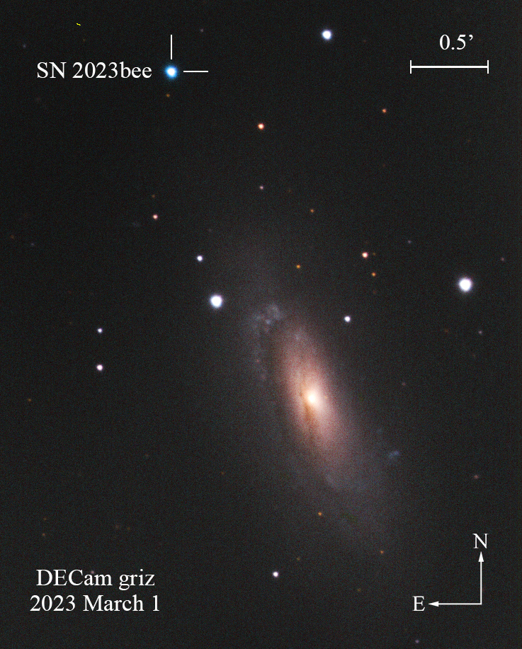
Figure 1: DECam composite $griz$ image stamp of SN 2023bee and its host NGC 2708 taken on 2023 Mar 1 UT, $\sim 10$ days after peak. The location of SN 2023bee is marked by white tick marks in the upper left corner.

2 Observations and Data Reduction

SN 2023bee was discovered by the Distance Less Than 40 Mpc survey (DLT40) (Yang et al., 2017; Tartaglia et al., 2018) on 2023 Feb 1 17:59:54.816 (MJD 59976.75) in the Clear band with an apparent magnitude of $17.26\pm 0.04$ mag (Andrews et al., 2023). SN 2023bee occurred at coordinates $\alpha=\rm 08^{h}56^{m}11.63^{s}$, $\delta=-03{\arcdeg}19{\arcmin}32.06{\arcsec}$ (J2000.0) and was spectroscopically classified as a SN Ia by Hosseinzadeh et al. (2023b). SN 2023bee is located at a distance of 93.97″ from the center of its host galaxy NGC 2708, which is an intermediate spiral galaxy at $z=0.0067\pm 0.0005$ and distance modulus $\mu=32.5\pm 0.2$ mag (Pisano et al., 2002). Given the large separation between SN 2023bee and its host, the host extinction is likely to be negligible. Throughout this paper, we use the Milky Way extinction of $E(B-V)_{MW}=0.0145$ from the extinction map described in Schlafly & Finkbeiner (2011).

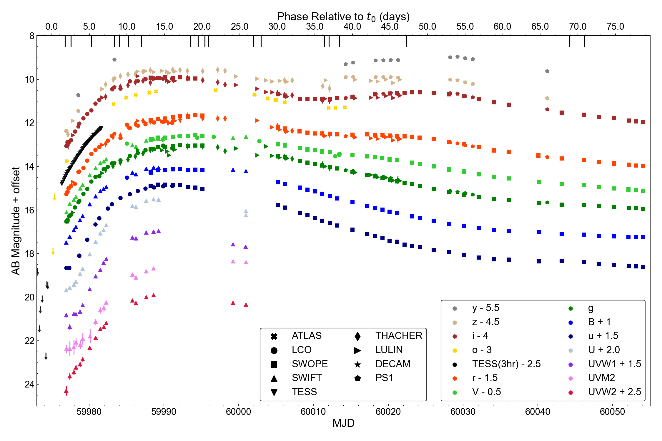
Figure 2: Multi-band light curves of SN 2023bee. The TESS data have been binned in 3-hour bins to increase the signal-to-noise ratio. The rest-frame phases relative to the inferred time of first light $t_{0}$ (see Section 3.2) from TESS are labeled at the top. The down arrows mark the non-detections at the position of SN 2023bee in different bands and epochs. The times when optical spectra were taken are labeled as black ticks at the top.

2.1 Photometry

TESS observed the rise of 2023bee during sector 61, in CCD 1 of camera 1. TESS features a broadband filter that covers the $r,i,z$ and $y$ bands with a wavelength range of 5802.57 to 11171.45 Å. We create a $90\times 90$ pixel² target pixel file, centered on 2023bee, from the calibrated TICA (Fausnaugh et al., 2020) full frame images (FFIs) with TESScut. The target pixel file was reduced with the standard TESSreduce pipeline, which accounts for image alignment, the scattered light background, and image artifacts to produce differenced images. We then conduct a secondary background subtraction by subtracting the median counts of each column from each pixel in that column, for every differenced image.

The baseline flux is estimated by the median value between MJD 59969.2 and 59974 when the background is stable and no SN flux is present. Between MJD 59974.5 and 59976.3 the TESS measurements are significantly compromised by scattered light in the background and thus are excluded from further analysis. The complete TESS light curve along with details of the method and criteria we used to determine the compromised MJD range are described in Appendix.

We calibrate the TESS counts of SN 2023bee to physical AB magnitudes with the spectrum taken on MJD 59977.56 (see Fig. 9). This spectrum is first calibrated using the LCO $g,r$, and $i$ measurements taken at the same night. Then we calculate a synthetic TESS magnitude, which we compare to the instrumental magnitude of the TESS measurement at the same time to compute the zeropoint. For this process, we use the pyphot package (Fouesneau, 2022) and the bandpasses available from the Spanish Virtual Observatory (SVO) (Rodrigo et al., 2012; Rodrigo & Solano, 2020). We find the zero-point of TESS to be $zp_{TESS}=26.16\pm 0.02$ mag.

We also observed SN 2023bee in $griz$ with DECam at the CTIO 4 m Blanco telescope (DePoy et al., 2008; Flaugher et al., 2015) and the PanSTARRS1 (PS1) telescope (Chambers et al., 2016) as part of the Young Supernova Experiment (Jones et al., 2021; Aleo et al., 2022). Standard reductions for the DECam and PS1 images are performed by the NOIRLab community pipeline (Valdes et al., 2014) and the PS1 image Image Processing Pipeline (IPP), respectively (Magnier et al., 2020a, b, c; Waters et al., 2020). These images are then taken as input to the photpipe pipeline (Rest et al., 2005, 2014), which re-determines the zero points by comparing DoPHOT PSF photometry from each image to the Pan-STARRS DR1 catalog (Flewelling et al., 2020), convolves and subtracts a template image from the survey image, and performs forced photometry on the resulting difference images to create SN light curves. Fig. 1 shows a DECam $griz$ color image taken on 2023 Mar 1 UT.

We observed SN 2023bee with the Las Cumbres Observatory (LCO) 1 m telescope network in $uBVgriz$ bands, the 1 m telescope at Lulin Observatory using the Lulin Compact Imager, and with the Thacher 0.7 m telescope in Ojai, CA from 2 February to 11 March 2023 in the $griz$ bands (Swift et al., 2022). Using the photpipe imaging and reduction pipeline (Rest et al., 2005, 2014), we performed bad-pixel masking, reprojecting the data to a common pixel scale and pointing center using SWarp (Bertin, 2010), photometry with DoPhot (Schechter et al., 1993), and photometric calibration using the Pan-STARRS 3$\pi$ (Flewelling et al., 2020) and SkyMapper photometric catalogs (Onken et al., 2019). The final photometry of SN 2023bee was obtained by performing forced point-spread function (PSF) photometry at the average position of the source across all of our images.

Additionally, we observed SN 2023bee in optical $uBVgri$ bands with the Swope 1 m optical telescope located at Las Campanas Observatory, Chile, as part of the Precision Observations of Supernova Explosions (POISE) (Burns et al., 2021). As described in Kilpatrick et al. (2018), all image processing and optical photometry was performed using photpipe (Rest et al., 2005), flat-fielding, image stitching, and photometric calibration. $BgVri$ photometry were calibrated using standard sources from the Pan-STARRS DR1 catalog (Flewelling et al., 2020), while the u-band data were calibrated using SkyMapper $u$-band standards (Onken et al., 2019), transformed into the Swope natural system (Krisciunas et al., 2017) with the Supercal method (Scolnic et al., 2015).

In addition, the Neil Gehrels Swift Observatory (Swift) observed SN 2023bee from 1–26 February 2023. We downloaded all processed Ultraviolet Optical Telescope (UVOT) data from NASA/HEASARC and performed forced aperture photometry at the location of SN 2023bee using methods in heasoft (v6.28; Nasa High Energy Astrophysics Science Archive Research Center (2014), Heasarc) and calibrated using the latest Swift/UVOT sensitivity files.

SN 2023bee was also observed by ATLAS, a project using four $0.5\,{\rm m}$ telescope systems installed on Haleakala (Hawaii), Mauna Loa (Hawaii), Las Campanas (Chile), and Sutherland (South Africa) to discover and monitor solar system objects. ATLAS observes in cyan (c) and orange (o) filters (Tonry et al., 2018). The ATLAS images are processed as described in Tonry et al. (2018), and then photometrically and astrometrically calibrated using the RefCat2 catalog (Tonry et al., 2018). Template generation, image subtraction procedures, and photometric measurements are carried out following Smith et al. (2020). We obtain forced photometry using the ATLAS forced photometry server (Shingles et al., 2021). The forced photometry light curve is then cleaned up and the average flux for each night is calculated using ATClean Rest et al. (2021, 2023).

2.2 Spectra

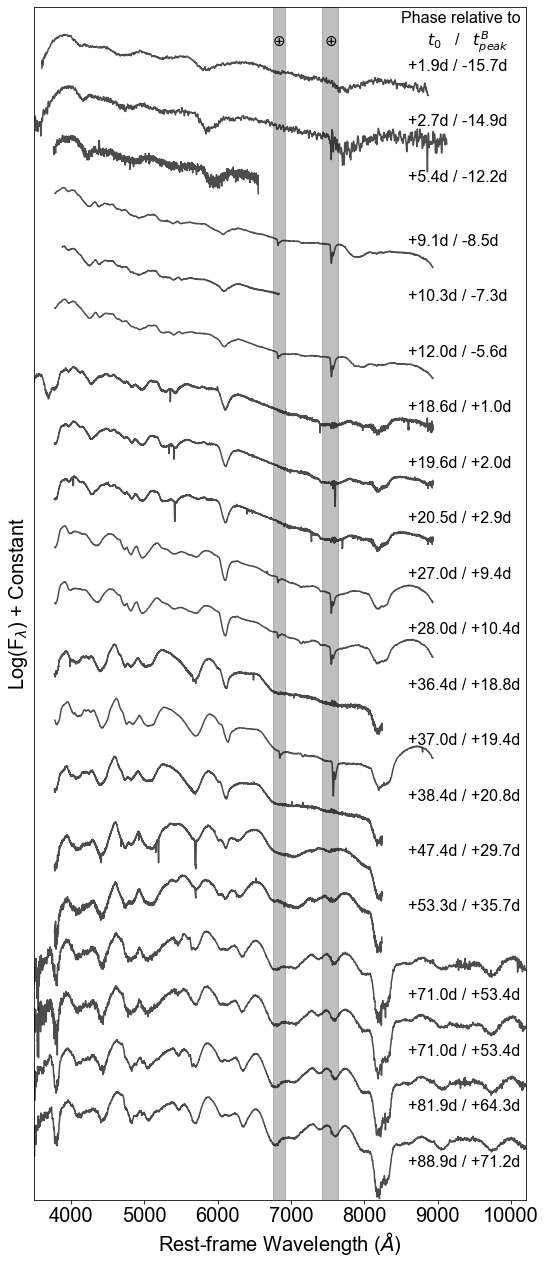
Figure 3: Optical spectra series of SN 2023bee. Phases relative to $t_{0}$ and $t_{peak}^{B}$ are labeled above each spectra. The telluric lines has been marked with the Earth ($\oplus$) symbol. All the spectra have been normalized and shifted for clarity.

We collect 20 optical spectra from various sources, which include two publicly available spectra from the Transient Name Server (Zhai et al., 2023; Hosseinzadeh et al., 2023b) obtained with the Lijiang 2.4m telescope and 2-meter Faulkes Telescope South (FTS) at Siding Spring Observatory (SSO) at early time, 7 spectra from Wide-Field Spectrograph (WiFeS) on the SSO 2.3m telescope, 6 spectra with the Alhambra Faint Object Spectrograph and Camera (ALFOSC) on the Nordic Optical Telescope (NOT) at La Palma, 3 spectra with the Kast spectrograph on the Lick 3 m (Shane) telescope, 1 spectrum with the Kitt Peak Ohio State Multi-Object Spectrograph (KOSMOS, Martini et al. 2011) on the Astrophysical Research Consortium (ARC) 3.5-meter Telescope at Apache Point Observatory (APO), and 1 spectrum with the Goodman spectrograph on the 4.1-meter Southern Astrophysical Research (SOAR) Telescope.

The ALFOSC spectra were taken using grism 4 and a 1.0" slit, aligned along the parallactic angle, under clear observing conditions and good seeing ($<$1.5"). The spectra were reduced with a custom pipeline running standard pyraf procedures. The Kast and Goodman spectra were reduced through the UCSC Spectral Reduction Pipeline (Siebert et al., 2020), a custom data-reduction pipeline based on procedures outlined by Foley et al. (2003), Silverman et al. (2012), and references therein. The WiFeS spectra were taken using a RT-560 beam splitter, a B3000 and R3000 diffraction gratings and Y=2 binning read out corresponding to a $1\times 1$ arcsec spaxel. Each observation was reduced using PyWiFeS (Childress et al., 2014) producing a 3D cube file for each grating that has had bad pixels and cosmic rays removed. Spectra were extracted using QFitsView and a similar aperture to the seeing on the night (average seeing of $\sim$ 2"), while for background subtraction we extract a part of the sky that is isolated from the source. The KOSMOS spectra were reduced through the standard KOSMOS pipeline. The spectroscopic time series is shown in Fig 3 and information of the spectra are listed in Table 3 in Appendix. A comparison to spectra from other SNe at similar phases is shown in Fig. 9

Parameters	SALT3	Hsiao
$t_{0}/t^{B}_{peak}$ (MJD)	$59973.796\pm 0.006$	$59992.354\pm 0.005$
$x_{0}$	$0.1017\pm 0.0001$	-
$x_{1}$	$1.399\pm 0.009$	-
$c$	$-0.0902\pm 0.0008$	-
Amplitude	-	$5.603\pm 0.003\times 10^{-6}$

Table 1: Best-fit results for SALT3 and Hsiao et al. (2007) models with SNCosmo. Note that SALT3 uses time of first light $t_{0}$ while Hsiao07 model uses time of B-band peak $t^{B}_{peak}$.

3 Analysis

3.1 Photometric Properties

In this section, we analyze the observed light curve of SN 2023bee and compare it to various models. First, we fit the multiband light curves to the SALT3 (Kenworthy et al., 2021; Pierel et al., 2022) model with SNCosmo (Barbary et al., 2016), excluding the UV and TESS data due to its poor coverage in these wavelength ranges. The best-fit results for these two models are shown in Table 1. The $B$-band peak is estimated to be $t_{peak}^{B}=59992.58$ MJD with $m_{peak}^{B}=13.041\pm 0.001$ mag, corresponding to a $M_{peak}^{B}=-19.6\pm 0.2$ mag. This corresponds to a $\Delta m_{15}$(B)$=0.788\pm 0.002$ mag. Combining these properties, SN 2023bee is in the subclass of relatively slow and luminous SNe Ia that are still considered normal SN Ia (Phillips, 1993; Hicken et al., 2009), similar to SN 2021aefx (Hosseinzadeh et al., 2022; Ashall et al., 2022).

We also fit the multi-band light curves using the spectral template model of Hsiao et al. (2007), which offers better coverage in the near-infrared (NIR) and allows us to include the exquisitely sampled TESS data in the fit. The inferred time of the peak is $t_{peak}^{TESS}=59991.8$ MJD with $m_{peak}^{TESS}=13.68$ mag, and we will adopt these values in the later analysis.

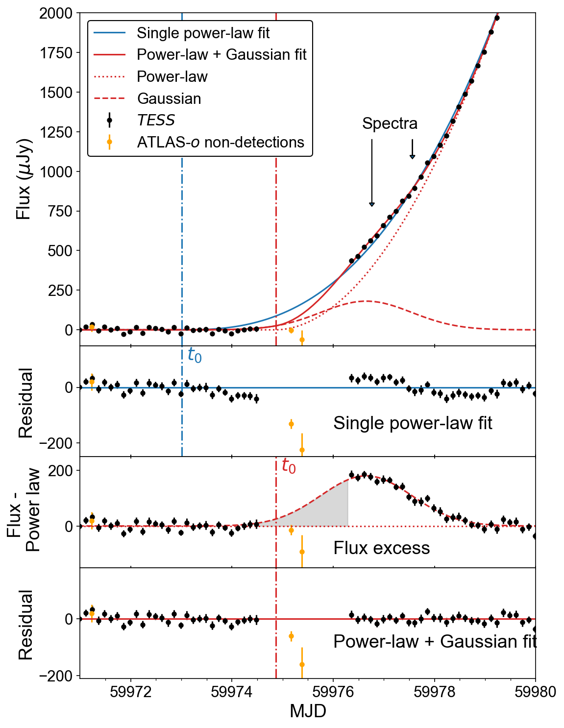
Figure 4: Top: the early TESS light curve of SN 2023bee fitted to a single power-law (blue solid) and power-law plus Gaussian (red solid). The power law and Gaussian component are plotted as dotted and dashed lines separately for clarity. The inferred $t_{0}$ of each power-law is plotted as a vertical line in the corresponding color. Down arrows denote the times when early spectra are obtained. Middle: residuals with regard to the single power-law fit. Bottom panels: the excess as flux subtracted by the power-law component in the power-law + Gaussian fit, and residuals with regard to the complete fit. The atlas-$o$ band non-detections are also included for comparison. In the shadowed region where the flux excess starts to rise, the Gaussian component is less constrained due to the lack of data, and thus may not correctly reflect the light curve during this period.

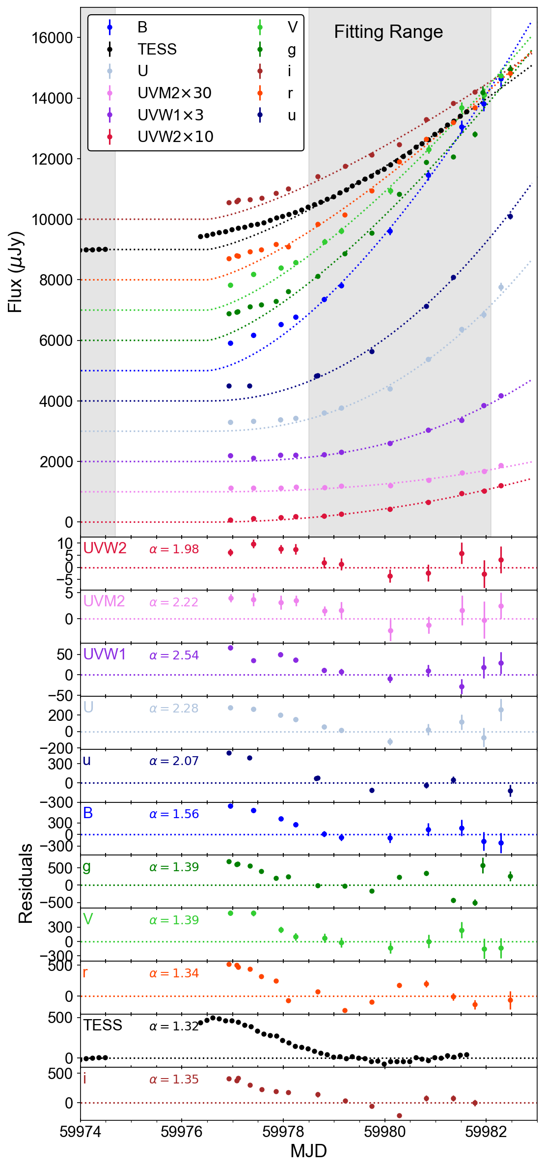
Figure 5: Partial power-law fit of the multi-band light curve of SN 2023bee and the residuals in different bands. The fitting range is marked as the grey region in the top panel. The best-fit power-law index is listed in individual residual plots. For better visualization, the data in the UV bands are rescaled as marked in the legend.

3.2 Early rise and excess

As seen in Fig. 2, the UV light curves from UVM2 to $U/u$ bands have a relatively flat rise within the first $\sim 3$ days, indicating the existence of an early excess. However, in optical bands, the signature of early excess is more subtle and cannot be easily distinguished from the power-law rise of the SN itself. Thus, we make use of a few different power-law fitting schemes to verify the existence of the excess and determine the timepoint when the first optical emission emerge, i.e. the time of first light $t_{0}$ in optical bands.

TESS covers SN 2023bee from the pre-explosion stage until MJD 59981.67, when the SN reaches $\sim$30% of the peak flux as estimated based on the $r$ and $i$ bands. Due to the influence of scattered light in the background, the TESS light curve around the time of the explosion is severely polluted, making it impossible to identify the first real detection and constrain $t_{0}$ with high precision. However, there are non-detections in the $o$ band on MJD 59975.17 and 59975.37 with upper limits of $m_{o}>20.76$ and $18.26$ mag respectively. These non-detections give a strong constraint on $t_{0}$. The first detection in $o$ band appeared on MJD 59977.01 with $m_{o}=16.76\pm 0.02$ mag. Due to the lack of more $o$-band during the first days after explosion, it is impossible to fit a power-law to the $o$-band data directly.

To identify whether there is excess flux in addition to the the power-law rise, and constrain $t_{0}$, we fit the TESS light curve with two models: a single power-law rise,

$$f(t)=A_{pl}(t-t_{0})^{\alpha},$$ (1)

and a power-law rise with a Gaussian function near the time of first light,

$$f(t)=A_{pl}(t-t_{0})^{\alpha}+\frac{A_{G}}{\sigma\sqrt{2\pi}}e^{-(t-\mu)^{2}/2\sigma^{2}}.$$ (2)

In the two equations, $t_{0}$ denotes the time of first light, $A_{pl}$ and $\alpha$ denote the scale and the index of the power-law, and $A_{G}$, $\mu$ and $\sigma$ denote the scale, center, and width of the Gaussian component respectively. We note that the second scenario is unphysical since this model will never have zero flux. Nevertheless, we examine it to understand the morphology of the early light curve with a simple few-parameter function.

We perform a least-square fit with lmfit package (Newville et al., 2023). The fitting results are shown in Figure 4 and Table 2. To avoid overfitting, the Bayesian Information Criteria (BIC) is used to judge the goodness-of-fit in order to balance the deviation of fit and the number of parameters used.

There are a few factors that make the power-law + Gaussian fit more preferable. First of all, this double-component fit has significantly lower BIC. Secondly, while the deviations from a single power-law are barely within $3\sigma$ limit in residual space for a given single flux measurement, there is a noticeable ‘S’-shape during the first few days, a characteristic sign of excess flux that cannot be fit with a single power-law with high significance (e.g. see Dimitriadis et al., 2019a, 2023). In addition, we have $o$-band non-detections in the TESS gap (see orange symbols in Fig. 4). We can expect that the atlas-$o$ light curve is very similar to the TESS light curve, since their wavelength ranges are similar. The atlas-$o$ non-detection on MJD 59975.17 deviates from the single power-law fit with $>$5$\sigma$, which is another strong indication that the single-power law fit is not correct and the inferred $t_{0}$ is significantly biased toward early times.

For the power-law + Gaussian fit, we obtain $t_{0}=59974.86\pm 0.26$ and we adopt this value in the following analysis. Note that in Figure 4 the model flux is non-zero before $t_{0}$ due to the tail of the Gaussian profile. Such a bias can be caused by the fact that the excess flux is likely asymmetric and cannot be fully described by a simple Gaussian. In principle this bias can be minimized by using a skewed Gaussian as shown in Dimitriadis et al. (2019a), but the lack of data at early times corresponding to the first half of the Gaussian profile makes it difficult to constrain this asymmetry. Furthermore, the influence of this Gaussian tail is negligible in the residuals Therefore, the skewed Gaussian fit gives indeed a higher BIC and is thus less useful in this case.

To see whether the flux excess exists in other bands, we also fit part of the multi-band light curves with the same $t_{0}$ and different power-law indexes, excluding the earliest phases when the flux excess is still significant compared to the power-law component. To find the best fitting range, we adopt an iterative fitting approach similar to Dimitriadis et al. (2019a), using a fitting window with variable starting and ending times. To ensure adequate data points in multiple bands are included, the fitting goes through the starting time in between the first detection until when the TESS flux reaches $\sim 15\%$ of the estimated peak, and the ending time is set to be in between MJD 59982 to 59983.5 when the extrapolated power-law rise of TESS light curve lies in between $30\%$ to $40\%$ of the estimated peak. The MJD range with lowest reduced-$\chi^{2}$ is from 59978.5-59982.1 and is thus selected for the power-law fit, marked as the grey region in Figure 5 along with the best-fit results and residuals. The excess flux is clearly visible in all bands from the UV to $i$ band.

The fitted power-law indices are between 1.35 and 1.6 in the optical, which is significantly smaller than the power-law indices close to 2 found in SN Ia without excess flux (Hayden et al., 2010; Olling et al., 2015). However, it is likely that at least some flux from the excess contributes to the total flux in the fitting region, affecting the exact power-law index. When we simultaneously fit the excess flux and power-law rise using theoretical models for the excess (see Section 4), the power-law indices for optical bands is closer to the typical value of $2$ (Hayden et al., 2010; Olling et al., 2015).

model	$t_{0}$ (MJD)	$\alpha$	$A_{pl}(\mu$Jy)	$A_{G}(\mu$Jy)	$\mu$ (MJD)	$\sigma$ (days)	reduced $\chi^{2}$	BIC
power-law	$59973.00\pm 0.15$	$2.59\pm 0.06$	$17.4\pm 3.1$	-	-	-	$518.1$	$503.8$
power-law + Gaussian	$59974.86\pm 0.26$	$1.93\pm 0.09$	$115\pm 29$	$400\pm 100$	$59976.65\pm 0.08$	$0.90\pm 0.09$	$205.5$	$440.7$

Table 2: Different power-law fitting results on TESS light curve of SN 2023bee.

3.3 Comparison with Other SNe Ia in TESS and Kepler

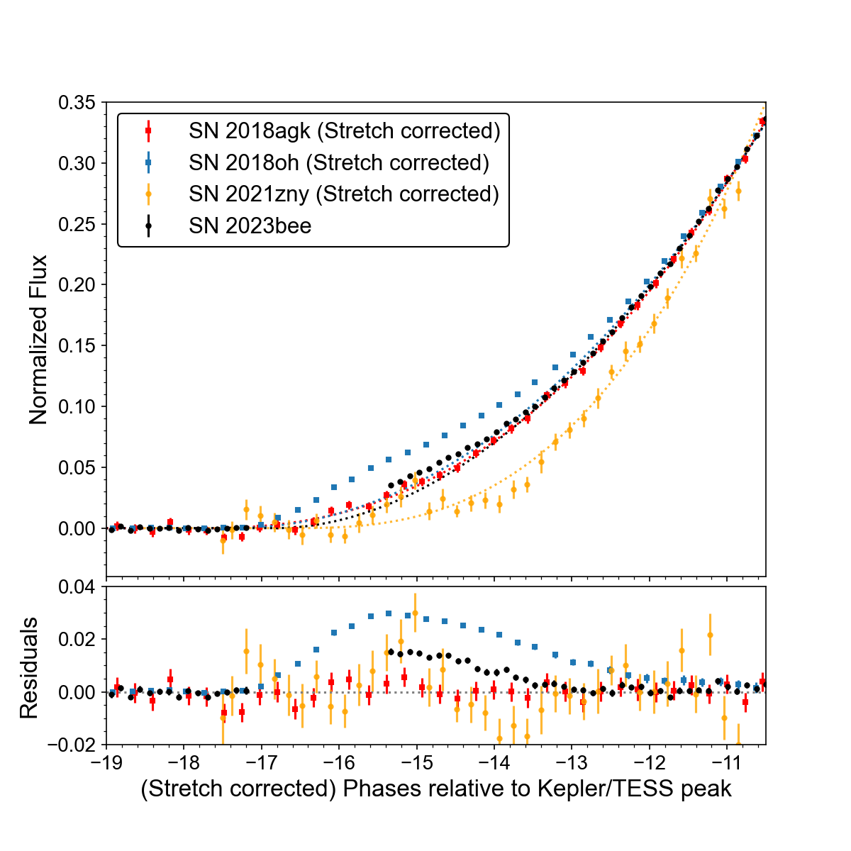
Figure 6: Top: Comparison of SN 2023bee (black) with other well-studied SNe Ia with high cadence early light curves from Kepler and TESS, including SN 2018oh (blue), SN 2018agk (red) and SN 2021zny (yellow). The light curves of the comparison SNe Ia have been ‘stretch-corrected’ to match the rise of SN 2023bee, with regard to their rise time from $30$% of the peak flux to the peak in the Kepler/TESS bands. Power-law fits to part of the light curves are also shown, for which the details are described in the main text. Bottom: Residuals relative to the power-law fits for these SNe Ia in Kepler and TESS.

We further compare the early TESS light curve of SN 2023bee to other well-studied SNe Ia with high cadence light curve from Kepler and TESS. Our sample includes SN 2018oh, a normal SN Ia with clear early excess in Kepler (Dimitriadis et al., 2019a; Shappee et al., 2019), SN 2018agk, a normal SN Ia with a smooth power-law rise in Kepler (Wang et al., 2021), and SN 2021zny, a super-$M_{ch}$ SN Ia with short duration excess captured by TESS (Dimitriadis et al., 2023). We adopt the partial power-law fits directly from the individual analyses.

We note that the sample shows a large spread in rise times. SN 2023bee has a relatively short rise time $t_{\textrm{rise}}=16.8$ days in the TESS band, while SN 2018oh and SN 2018agk have $t_{\textrm{rise}}=18.2$ and $18.1$ days respectively, similar to the majority of normal SNe Ia (e.g., see Hayden et al., 2010; Miller et al., 2020b). SN 2021zny, in contrast, has a significantly longer rise time $t_{\textrm{rise}}\gtrsim 21$ days. We therefore ‘stretch correct’ the comparison set of SNe Ia with a stretch factor so that the other SNe fit best the rising arm of SN 2023bee from 30% of the peak flux to the peak. As shown in Figure 6, the power-law rise of SN 2023bee, SN 2018oh, and SN 2018agk align very well after ‘stretch correction,’. However, SN 2021zny is an outlier, and has a peculiar rise compared to the other SNe in this sample. The excess in the TESS light curve of SN 2023bee has similar morphology to that of SN 2018oh in the Kepler band, though $\sim$50% weaker and $\sim$1 day shorter. The excess of SN 2021zny, on the other hand, has a shorter duration and more abrupt evolution. It can also be seen from the residual plot that if the data for SN 2023bee had a similar S/N to that of SN 2018agk, the early excess would still be detectable.

3.4 Color Evolution

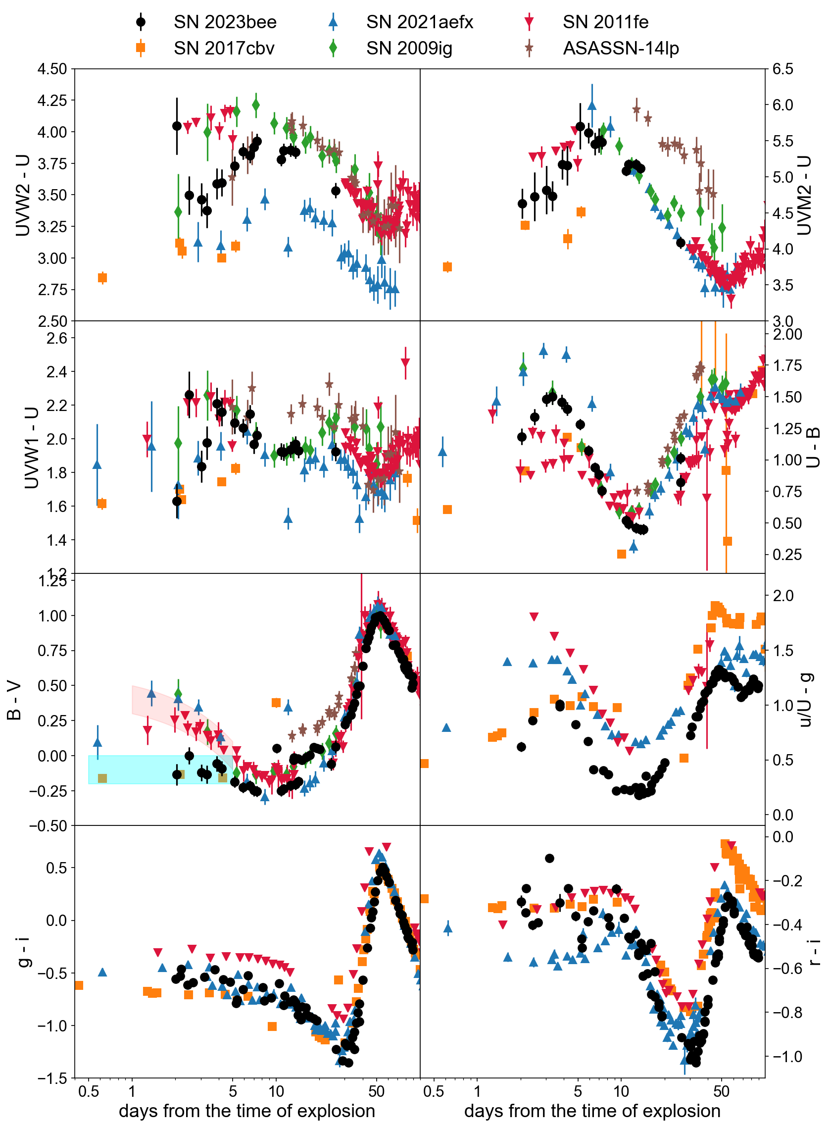
Figure 7: Extinction-corrected color evolution of SN 2023bee in multiple bands, in comparison with normal SNe Ia (SN 2011fe, SN2009ig and ASASSN-14lp) and SN Ia with bump in UV (SN 2017cbv, SN 2021aefx). All the magnitude have been converted into AB-magnitude system. In $U-B$, $B-V$ and all UV bands, the only data for SN 2023bee at early time are from Swift. The cyan and red region in $B-V$ plot outline the evolution of ‘early blue’ and ‘early red’ subgroups as defined in Stritzinger et al. (2018). The synthetic $ugri$ photometry of SN 2011fe are calculated from the photometrically calibrated spectra series from Pereira et al. (2013).

Figure 7 shows the UV and optical color evolution of SN 2023bee at early phases, in comparison to other SNe Ia with excesses flux such as SN 2017cbv (Hosseinzadeh et al., 2017) and 2021aefx (Hosseinzadeh et al., 2022; Ashall et al., 2022), as well as other normal SNe Ia without excess including SN 2009ig (Foley et al., 2012), SN 2011fe (Nugent et al., 2011) and ASASSN-14lp (Shappee et al., 2016). The color curves have been dereddened and converted to the AB magnitude system. Phases are relative to the time of first light estimated in the respective studies of each SN.

Overall, in the UV bands, SN 2023bee has an intermediate color in between SNe Ia with and without excesses, bluer than normal SNe Ia and redder than SN 2017cbv and 2021aefx. Milne et al. (2013) separated SNe Ia based on their UV colors at early times, and SN 2023bee would be NUV-blue based on this classification. However, NUV-blue SNe tend to have lower ejecta velocities than NUV-red SNe (Milne et al., 2015), perhaps making SN 2023bee an outlier. Similar to SN 2017cbv and SN 2021aefx, SN 2023bee also has a rapid trend in UVW1-$U$, $U-B$ and $u-g$ toward redder colors when the early excess is present. Afterward, the color evolution of SN 2023bee in UV resembles a normal SN Ia as SN 2009ig and SN 2011fe, while SN 2017cbv and SN 2021aefx are significantly bluer around the same phases, while in some optical bands including $u/U-g$ and $r-i$, SN 2023bee is marginally bluer in later phases, similar to SN 2021aefx.

In the $B-V$ plot in Fig. 7, the regions correspond to the ‘early red’ and ‘early blue’ groups as defined by Stritzinger et al. (2018) have been highlighted, and SN 2023bee falls in the ‘blue’ group where the $B-V$ color is relatively constant and blue, similar to SN 2017cbv. Given the observed colors across all of these bands, it is likely that there is a continuum from the ‘blue’ to the ‘red’ SNe Ia rather than two distinct groups, in agreement with the conclusion of Bulla et al. (2020).

3.5 Spectroscopic Evolution

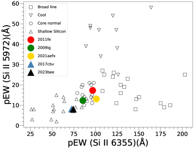
Figure 8: Si II $\lambda$5972 and Si II $\lambda$6355 pseudo-equivalent-width (pEW) measurements for a sample of SN Ia from Branch et al. (2009) (empty symbols) and for SNe Ia of interest (filled symbols). This parameter space defines subclasses of SN Ia (Branch et al., 2006): “shallow silicon,” “core normal,” “cool,” and “broad line” . SN 2023bee falls within the “shallow-silicon" subclass and is similar to another early excess SN Ia, SN 2017cbv.

Two valuable spectra were obtained during the early flux excess. In Figure 9, we compare them with other SNe Ia, including two SNe Ia without an early flux excess (SN 2009ig, Foley et al. 2012 and SN 2011fe, Parrent et al. 2012) and one SN Ia with bright UV early excess (SN 2017cbv, Hosseinzadeh et al. 2017 and SN 2021aefx, Hosseinzadeh et al. 2022; Ashall et al. 2022). The displayed spectra have all been normalized to the continuum between $6250-6400$ Å for clarity. At early times ($<$5.5d after the time of first light), SN 2023bee is most similar to SN 2017cbv with similar continuum and shallow absorption features, but with significantly higher velocity ($v_{\textrm{Si II}}\approx 24,000$ km s^-1) in general. Each of these SNe displays peculiar absorption near the red wing of Ca H&K, which has been interpreted as the result of high velocity Si II $\lambda$4130 blending with Ca H&K (Foley et al., 2012).

A notable difference between SN 2023bee and SN 2017cbv compared to other SNe Ia without an early flux excess is their significantly weaker absorption features in spectra obtained within a few days of explosion. This difference is particularly striking in the Si II $\lambda$6355, C II $\lambda$6580 and Ca II NIR triplet features with SNe 2017cbv and 2023bee having smaller equivalent widths than the comparison SNe. Since the same lines are present in all spectra with roughly the same line ratios, it is unlikely that there are significant differences in the abundance of intermediate-mass elements in the outer layers of these SNe. Contrastingly, only carbon and oxygen lines were detected in the earliest spectra of SN 2020esm, suggesting a significantly different composition than most SNe Ia (Dimitriadis et al., 2022). Instead, a difference in the equivalent widths may be the result of a stronger continuum corresponding to the excess flux at these times. On the other hand, the spectra of SN 2021aefx during the early excess phase are analogous to SN 2009ig and exhibit distinct line strength and SED compared to SN 2023bee and SN 2017cbv, potentially indicating the difference in the origin of early excess in optical bands. After the excess flux subsides, the equivalent widths of SNe 2023bee are closer to the comparison sample.

At maximum light, SN 2023bee appears to have the highest degree of similarity with SNe 2009ig and 2017cbv, having shallow Si II features. The maximum-light spectrum is generally consistent with those of other slow-declining SNe ($\Delta m_{15}$(B) < 0.9 mag), having shallow Si II $\lambda$5972 and a stronger peak on the blue side of Ca H&K. We compare the Si II absorption strength to other subclasses of SNe Ia in Figure 8. SN 2023bee clearly falls within the boundary of the “shallow-silicon" SN Ia subclass identified in Branch et al. (2006). Interestingly, SN 2017cbv, another early-excess SN Ia had very similar Si II absorption features to SN 2023bee at maximum light.

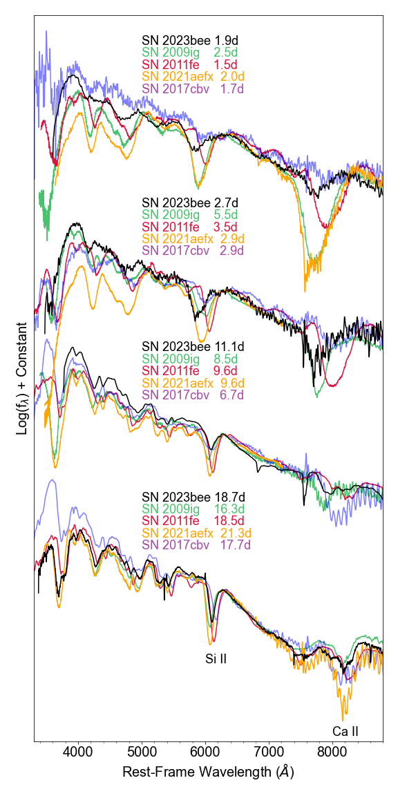
Figure 9: Comparison between spectra of SN 2023bee, SN 2009ig, SN 2011fe, SN 2017cbv and SN 2021aefx during the time of excess, rise, and around the peak. The phases relative to the inferred time of first light has been labeled around the spectra. The flux has been normalized to the continuum between $6250-6400$Å. Note that SN 2023bee has shallow absorption features, similar to SN 2017cbv, but with significantly higher velocity.

4 modeling

In this section, we discuss the different possible physical mechanisms that might explain the early excess flux, and the implications on the progenitor properties of SN 2023bee.

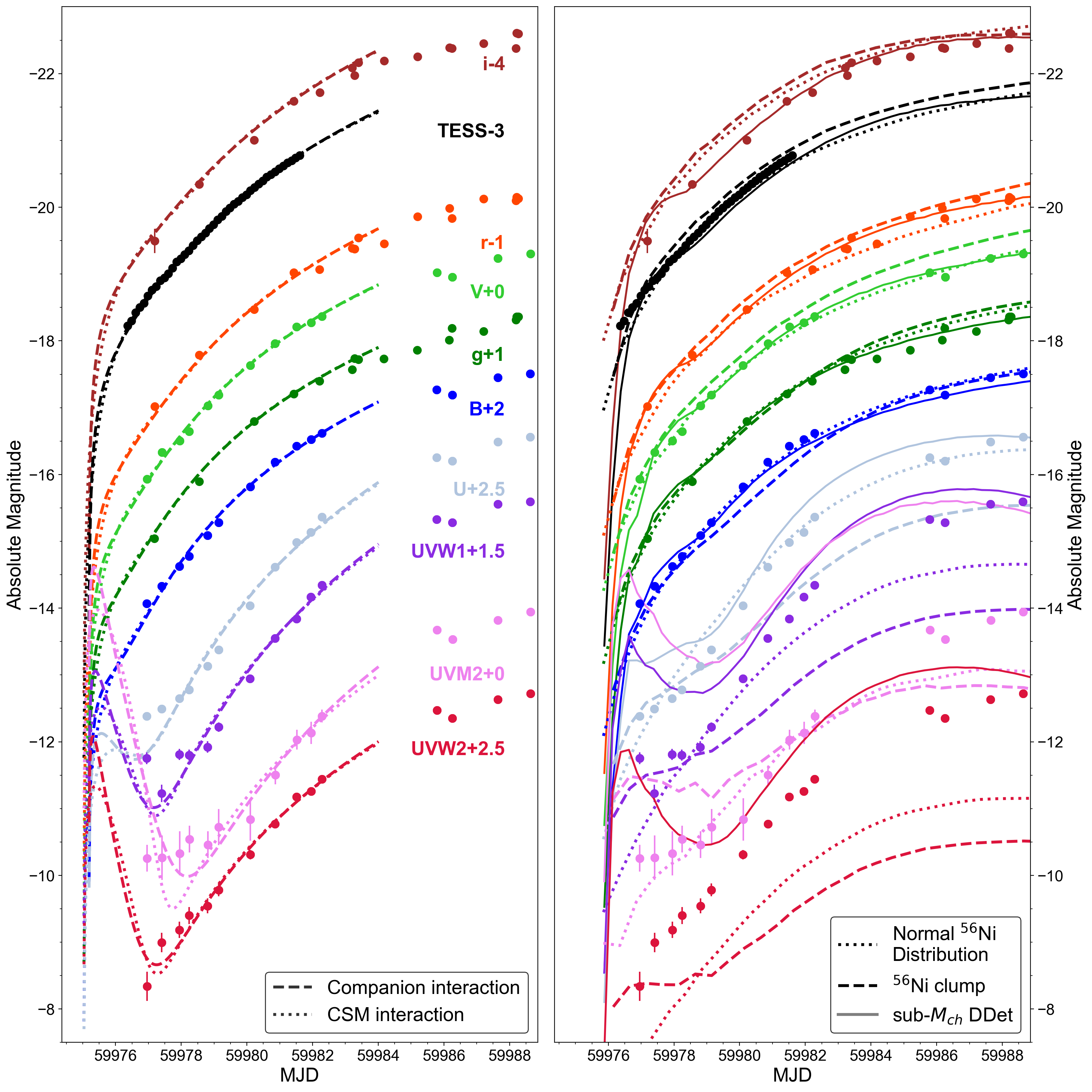
Figure 10: Multiband fit to the CSM-interaction and companion interaction models (left), and to the ⁵⁶Ni mixing and sub-$M_{ch}$ double-detonation models (right). A model with normal ⁵⁶Ni distribution from Magee et al. 2020 is included as a fiducial model for comparison. Color for different bands are labeled below each light curve in the left panel.

4.1 Companion Interaction

Kasen (2010) illustrates that when the SN ejecta collide with a non-degenerate companion, a blue and luminous excess flux will arise in the first few days after the explosion. The luminosity, duration, and SED of the excess are dependent on the binary separation, ejecta velocity, and viewing angle. Following the same fitting scheme as described in Dimitriadis et al. (2023), we fit the multi-band light curves of SN 2023bee to this companion-interaction model, adopting an ejecta velocity $v_{\mathrm{ej}}=12,500\>\mathrm{km\>s^{-1}}$ as measured from the peak spectrum, and assuming the underlying SN light curve to be power-law with the same time of the explosion but different indices in different bands. The time of first light $t_{0}$ and binary separation $a$ are the free parameters in the excess model. Due to the severe degeneracy between the viewing angle and other parameters, we assume a viewing angle $\theta=0^{\circ}$.

The best-fit result is shown in the left panel of Fig. 10 in comparison with the multiband light curve. While this model matches the rise of SN 2023bee relatively well, it has an early spike in the UV bands as a result of the high blackbody temperature, and thus fails to reproduce the relatively flat shape in multiple bands, especially for $U$, UVW1, and UVM2. One explanation for this discrepancy is that the models are not yet sophisticated enough to correctly predict the behavior in the bluer bands of the ejecta interactions with the companion star. For example, Kasen (2010) assume a blackbody SED for the excess flux, but UV line blanketing if any could dramatically change the evolution of early flux. New, improved companion interaction models would significantly help with the interpretation. Also, the power-law may not serve as a good approximation for individual SNe Ia in certain bands, especially in UV where there are less the SNe Ia with early coverage. Improving the modeling of early SNe Ia light curves in the different bands with new simulations and a larger data sample is necessary.

The best-fit binary separation is $a=2.27\pm 0.14R_{\odot}$. Given the condition that the single-degenerate systems are believed to be undergoing Roche-lobe overflow, the companion size can also be correlated with the binary separation (Eggleton, 1983). Assuming a typical mass of companion to be $1-6M_{\odot}$ we can estimate that $R\sim 0.8-1.15R_{\odot}$. These values are degenerate with the viewing angle so we are unable to give a conclusive answer on the companion parameters, but given the order of magnitude, this relatively small radius is in agreement with a main sequence star companion. This result is in agreement with the non-detection in the radio in Hosseinzadeh et al. (2023a), which indicates a low mass-loss rate and rules out most of the red-giant companions. The inferred $t_{0}=59975.18\pm 0.02$ MJD is also marginally in agreement with our value inferred from the power-law + Gaussian fit.

4.2 CSM Interaction

We also attempt to fit the multi-band light curves with a model similar to Ni et al. (2023b), Dimitriadis et al. (2023), and Srivastav et al. (2023), in which the early flux excess is powered by confined CSM close to the explosion site, approximated as a spherically symmetric envelope of mass $M_{\mathrm{env}}$ and radius $R_{\mathrm{env}}$ (see Piro (2015) for a complete presentation of the model). This model has successfully explained some relatively short and weak flux excesses, commonly seen in 03fg-like SNe (e.g. SN 2021zby), and possibly associated with double white dwarf merger events. Similar to our Kasen (2010) model fit, we use a power law as the underlying SN light curve. As no hydrogen has been identified in the spectra of SN 2023bee, we assume for the H-poor CSM an electron-scattering opacity of $\kappa=0.2\>\mathrm{cm^{2}\>g^{-1}}$, while for the ejecta mass and velocity, we use the canonical values of $M_{\mathrm{ej}}=1.4\>\mathrm{M_{\odot}}$ and $v_{\mathrm{ej}}=12,500\>\mathrm{km\>s^{-1}}$ as measured from the peak spectrum. Due to the lack of a robust estimate of the explosion date and the sparse coverage of the flux excess, we assume that the time of the onset of the CSM interaction coincides with the time of first light for each photometric band.

The best-fit parameters are $M_{\mathrm{env}}=0.05\pm 0.02\>\mathrm{M_{\odot}}$ and $R_{\mathrm{env}}=(6.5\pm 1.4)\times 10^{10}$ cm, and assuming a $\rho\sim r^{-3}$ density distribution for the envelope, we estimate $M_{\mathrm{CSM}}=0.3\pm 0.1\>\mathrm{M_{\odot}}$, with $t_{0}=59975.02\pm 0.06$ MJD. As can be seen from Fig. 10, similar to the companion interaction model, the CSM interaction model does not reproduce the relatively flat rise at early times. In fact, the CSM interaction model predicts an even more abrupt and shorter excess compared to the companion interaction model, making it less preferable in the case of SN 2023bee.

4.3 Sub-Chandrasekhar Double-detonation Models

In the sub–$\textrm{M}_{ch}$ DDet scenario, Polin et al. (2019) predict that the initial ignition of the thick He-shell on the surface will create radioactive material embedded in ashes in the outer layers of ejecta, which can cause early excess in the light curve. In general, a thicker He-shell will produce more radioactive isotopes and generate a stronger early excess. Due to the significant line blanketing in UV by these ashes, the early excess predicted by this DDet model tend to be red.

We tried fitting the data with all 39 1-dimensional models in the grid from Polin et al. (2019) using the least $\chi^{2}$ method to find the best match. Additionally we add two complementary parameters, the time of first light $t^{\prime}_{0}$ and distance modulus $\mu^{\prime}$, to account for the potential uncertainty in the phases and magnitudes. The range of $t^{\prime}_{0}$ and $\mu^{\prime}$ are set to be $\pm 2$ days around $t_{0}$ and $\pm 0.5$ mag around $\mu$. The best-fit model with the lowest $\chi^{2}$ is the one of a $1.1M_{\odot}$ WD and He-shell mass $M_{shell}=0.05M_{\odot}$, with $t^{\prime}_{0}=59975.75$ MJD and $\mu=32.35$ mag, and it is plotted as the solid line in the right panel of Fig. 10.

Overall, sub–$\textrm{M}_{ch}$ DDet model has a reasonable match to the light curve of SN 2023bee in most optical bands, but from $U$ to UV bands this model severely overpredicts the flux for both SN rise and the early excess. Similar to the companion interaction model and CSM interaction model, it prefers a ‘spike’-like excess and fails to reproduce the relatively smooth rise of SN 2023bee. On the other hand, the constant $g-r$ color curve and a relatively weak absorption feature in spectra at the early time agree with the prediction of a thick He-layer with $M\gtrsim 0.08M_{\odot}$ (see Fig. 6 and 8 in Polin et al., 2019). Still, a thicker He-layer will produce a more prominent early ‘spike’ in the UV, which can also be seen in the 12 models in Perets et al. (2019). Thus, it is difficult to reconcile the early color and spectral features with the flat UV rise of SN 2023bee in the sub$-\textrm{M}_{ch}$ DDet model. Another issue with sub$-\textrm{M}_{ch}$ DDet model is that the Si II$\lambda$5972 velocity and relatively high peak luminosity of SN 2023bee seems to fall into the range of the $\textrm{M}_{ch}$ group. We caution that the early UV observables will be highly sensitive to the treatment of the outer edge of the ejecta in simulations and modeling choices made in how to treat the surrounding medium. Better results with a flat rise in the UV can possibly be obtained by tracking the early outflow and unbound material during the first few orbital timescales in the Roche-Lobe Overflow stage until the merger in CO WD–HeCO WD DDet models (Zenati et al., 2019; Perets et al., 2019; Pakmor et al., 2021), or by taking line-of-sight effect into account with multi-dimensional models (Shen et al., 2021a, b).

4.4 ⁵⁶Ni Clump

We follow the method described by Magee et al. (2020) to find the best-matching ⁵⁶Ni distribution model among their 1-dimensional model suite. In addition, we also include the ⁵⁶Ni clump models presented by Magee & Maguire (2020) to determine whether they can provide a reasonable match to the early excess. Again, we allow for flexibility in the time of first light $t^{\prime}_{0}$ and distance modulus $\mu^{\prime}$. The best-matching ⁵⁶Ni distribution and ⁵⁶Ni clump models are EXP_Ni0.8_KE0.50_P4.4 (no excess) with $t^{\prime}_{0}=59975.3$ MJD and $\mu^{\prime}=32.15$ mag, and SN2017cbv_Ni0.04_Mean1.350_StdDev_0.180 (with excess) with $t^{\prime}_{0}=59975.4$ and $\mu^{\prime}=32.6$ mag, respectively. Both models are shown in Fig. 10.

As shown by Fig. 10, the ⁵⁶Ni clump model does not reproduce the shape of the early excess and generally shows a more prominent bump than what is observed in SN 2023bee, particularly in the UV bands. We note that this model was designed around reproducing the light curve of SN 2017cbv and therefore it is unsurprising that it does not provide perfect agreement with SN 2023bee. Models designed specifically around SN 2023bee likely could provide improved agreement in the optical bands and around maximum light, however, a suppression of flux in the UV is a natural consequence of large ⁵⁶Ni clumps in the outer ejecta as a result of significant line blanketing. Therefore while ⁵⁶Ni clump models adapted for SN 2023bee may be able to better match the shape of the early excess, it is unlikely they would simultaneously match the UV observations. Similarly, the ⁵⁶Ni distribution model shown in Fig. 10 provides reasonable agreement in the optical, but cannot reproduce the shape of the excess, which is expected for these models. Again we find that the model does not match the UV observations. This likely results from an extended ⁵⁶Ni distribution being preferentially selected in order to more closely match the excess at early times, which results in some UV line blanketing.

Based on the overall agreement of the light curve and strong disagreement in the UV bands, we find that the early excess in SN 2023bee is unlikely to have resulted from surface ⁵⁶Ni in a Chandrasekhar mass explosion. Further modeling exploring metallicity effects may provide improved agreement but is unlikely to overcome the significant discrepancies in the UV.

5 Discussion and Conclusion

In this paper, we presented early photometric and spectroscopic observations of SN 2023bee, including Swift UV and $10-$min cadence TESS light curves starting $\sim 2$ days after the time of first light. SN 2023bee has a relatively short rise time ($\sim 17$ days in TESS), high peak luminosity ($M^{B}_{peak}=-19.6$), and slow decline rate ($\Delta m_{15}(B)=0.788$). Most importantly, SN 2023bee shows clear evidence of an excess flux at early times detected in all bands, but most prominent in the UV. The two early spectra of SN 2023bee, taken within $\sim 3$ days after time of first light and at similar phases to the flux excess, show shallow high-velocity Si II and Ca II absorption features. These features are similar to those in SN 2017cbv, a Type Ia SN with an early excess flux, but distinctive from normal SNe Ia that do not show an early excess. They are also different to SN 2021aefx, which has an early bump, but shows strong Si II and Ca II absorption features at similar phases.

We use four different models to fit the early excess flux: companion interaction, CSM interaction, sub $M_{ch}$ DDet, and $M_{ch}$ ⁵⁶Ni clump models. None of these models manage to accurately reproduce the light curves in all bands. All models except for the ⁵⁶Ni clump model predict a sharp peak at the earliest phase in the UV, which is not observed in the early light curve of SN 2023bee. For both the ⁵⁶Ni clump model and the sub-$M_{ch}$ DDet model, the overall relative scaling between different bands does not fit the observed light curve. Similar challenges in modeling their light curves have been experienced in other SNe Ia with early UV excess such as SN 2017cbv (Hosseinzadeh et al., 2017) and SN 2021aefx (Hosseinzadeh et al., 2022; Ashall et al., 2022). The fact that none of the models explored here can adequately fit the observations over all passbands may have two explanations: either none of the physical mechanisms represent the true source of the excess and we must look for different explanations; or the current models are not sophisticated enough and/or do not explore a large enough parameter space to accurately reflect the complexity of the light curves. This is particularly true in the UV, where small changes are difficult to parameterize from initial conditions and, for example line blanketing, can lead to significant changes in the predicted spectra and photometry. More UV data, especially rapid UV spectroscopy from the Hubble Space Telescope within the first few days after explosion, like the UV spectra obtained during the rapid rise of SN IIP 2020fqv (Tinyanont et al., 2022), would uniquely probe the physical models and explain the nature of the excess.

Currently, even exquisite high-cadence multiband early observations of early excess SNe Ia such as the one presented here are unable to reliably distinguish between different progenitor scenarios. The nearby nature of these events makes it possible to observe them well into the nebular phase. Models that predict early flux excesses have distinct predictions for late time nebular emission. For example, narrow H/He features could be indicative of a single degenerate companion (Kasen, 2010; Kollmeier et al., 2019; Vallely et al., 2019; Prieto et al., 2020; Elias-Rosa et al., 2021), as seen in SN 2019yvq where strong [Ca II] emission could be the result of sub-$M_{ch}$ double detonation though the model prediction does not simultaneously match the early light curve(Siebert et al., 2020; Polin et al., 2019; Burke et al., 2021; Tucker et al., 2021), and [O I] emission, like that seen in the “02es-like" SN 2010lp and iPTF14atg maybe be produced in violent merger events (Taubenberger et al., 2013; Kromer et al., 2016). Furthermore, early flux excesses may occur at a higher rate in super-Chandrasekhar “03fg-like" SNe Ia (Jiang et al., 2018). These tend to have broad [O I] and sharp [Ca II] emission (Taubenberger, 2017; Dimitriadis et al., 2023). Given the remarkable photometric and spectroscopic similarity to SN 2017cbv and SN 2018oh, we may expect SN 2023bee to have similar behavior at late times. The nebular spectra of these events looked like a normal SN Ia (Tucker et al., 2019; Dimitriadis et al., 2019b) and had no evidence for H/He , [Ca II], or [O I] emission. With the James Webb Space Telescope, we can further explore the diversity in the mid/far-infrared spectra of SNe Ia at late phases (e.g., see Kwok et al., 2023; DerKacy et al., 2023), and search for further clues for the source of the difference between SNe Ia with and without early bumps.

There have now been a handful of normal SNe Ia with detected early excess flux (Dimitriadis et al., 2019a; Hosseinzadeh et al., 2017; Ashall et al., 2022; Hosseinzadeh et al., 2022). Notably, two of these SNe (SNe 2018oh and 2023bee) were observed by either Kepler or TESS. These SNe at 49 and 32 Mpc, respectively, are also among the closest SNe Ia observed by either observatory. The only comparably close SNe Ia in this combined sample (e.g., Olling et al., 2015; Fausnaugh et al., 2019, 2023, and other individual SNe discussed above) are SNe 2018fhw (Vallely et al., 2019) and 2018hib (Fausnaugh et al., 2019), at 74 Mpc and 66 Mpc, respectively. SN 2018hib did not have any indication of an early flux excess (Fausnaugh et al., 2019). While SN 2018fhw did not display early excess flux (Vallely et al., 2019), it has an abnormal nearly linear rise and its late-time spectra had hydrogen emission from circumstellar material, indicative of companion interaction (Kollmeier et al., 2019; Vallely et al., 2019). Therefore, half of the nearby SNe Ia observed by either Kepler or TESS have a flux excess with an additional object having other properties that indicate there may have been a flux excess if viewed from a different angle. Considering viewing angle effects, the physical mechanism that creates early flux excesses may be ubiquitous for all SNe Ia.

On the other hand, the detected rate of early excess drops dramatically when it comes to SNe Ia at higher redshift. Deckers et al. (2022) did a systematic analysis on the SNe Ia sample with early coverage from ZTF, and finds that 3 out of 30 SNe Ia with $z<0.07$ have detectable early excess, though there is large difference in data conditions such as signal-to-noise ratio and cadence between the brightest SNe Ia sample and the ZTF sample. Fausnaugh et al. (2023) did a systematic search for the early excess features in the early light curves of 74 SNe Ia in TESS Sector 1-50, only found 3 tentative candidates, and none of them are robust detection with the BIC test. The brightest SNe Ia with early excesses also show a wide variety of excess flux morphology and brightness relative to the SN brightness, e.g., a 50% difference in excess flux brightness between SN 2018oh and SN 2023bee, as well as differences in their early colors between SN 2017cbv, SN 2021aefx and SN 2023bee. The sample of high-cadence SN Ia from the space and the ground has grown significantly in the last few years, but we can only take advantage by pushing toward fainter SN Ia with better efficiency and contamination analyses that take the diversity of the bumps as well as the artifacts in the observational data fully into account.

Software and third party data repository citations

Fig. 11 shows the raw and 3-hour binned TESS light curve, and clearly the data around MJD 59975 become severely noisy. Fig. 12 shows the images before, during, and after this period, revealing that there is severe saturation in this part of the chip during this time. As can be seen from the bottom panel of Fig 11, those bad datapoints tend to have large scatter and thus can be characterised by the large sample standard deviation of flux measurements within each bin. Thus, we apply a cut based on the standard deviation of the binned data to remove those bad data in TESS light curve. Firstly, we selected a time range between MJD 59969.2 and 59974 in which the raw TESS light curve is stable to estimate the baseline flux and associated standard deviation $\sigma_{i}$ for each 3-hour $i$th bin. We calculate the mean $\bar{\sigma}$ and standard deviation $\sigma_{\sigma}$ of the $\{\sigma_{i}\}$ in this time range, and then we set the threshold for bad data as $\sigma_{i}>\bar{\sigma}+5\sigma_{\sigma}$. The threshold is plotted as the horizontal dotted line in the bottom panel of Fig 11, and visually it serves as a good cut in between the noisy and normal datapoints.

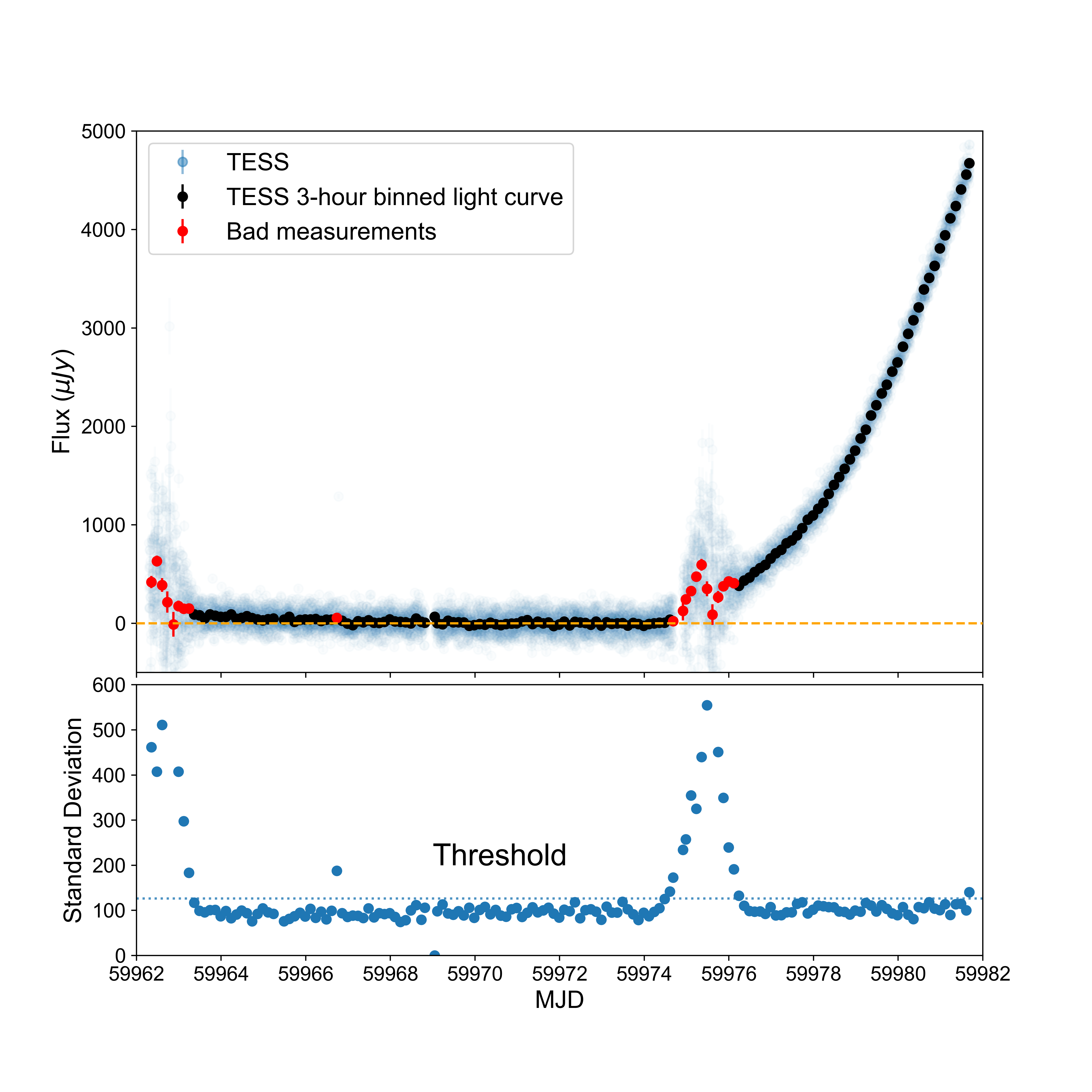
Figure 11: Top: the raw (blue) and 3-hour binned (black) TESS light curve of SN 2023bee. The red points denote the bad measurements, determined by a threshold characterized by their high uncertainty. Notice that before MJD 59969 there is a subtle trend in background flux, but between MJD 59969 and 59974 the background flux flattens out. Bottom: the standard deviations of light curve bins. The horizontal dashed line denotes the threshold defined as $\bar{\sigma}+5\sigma_{\sigma}$ for data between MJD 59969.2 and 59974 when the background flux is stable.

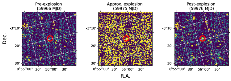
Figure 12: TESS image during the pre-explosion phase (left), around the time of first light when the background is saturated (middle), and during the rising phase when the background become stable again (right). Plots are in the same color scale and yellow are the saturated points.

Obs Date	MJD	Phase	Telescope	Instrument
(UT)		(Rest-Frame Days)
2023-02-01	59976.76	-15.74	Lijiang-2.4m	YFOSC
2023-02-02	59977.56	-14.94	FTS	FLOYDS-S
2023-02-05	59980.28	-12.23	APO-3.5m	KOSMOS
2023-02-08	59984.04	-8.50	NOT	ALFOSC
2023-02-10	59985.26	-7.29	SOAR	GOODMAN
2023-02-11	59986.96	-5.59	NOT	ALFOSC
2023-02-18	59993.59	1.01	SSO-2.3m	WiFeS
2023-02-19	59994.58	1.99	SSO-2.3m	WiFeS
2023-02-20	59995.47	2.88	SSO-2.3m	WiFeS
2023-02-20	59995.96	3.36	NOT	ALFOSC
2023-02-27	60002.01	9.38	NOT	ALFOSC
2023-02-27	60002.99	10.36	NOT	ALFOSC
2023-03-08	60011.43	18.76	SSO-2.3m	WiFeS
2023-03-09	60012.05	19.38	NOT	ALFOSC
2023-03-10	60013.47	20.79	SSO-2.3m	WiFeS
2023-03-19	60022.47	29.74	SSO-2.3m	WiFeS
2023-03-25	60028.42	35.66	SSO-2.3m	WiFeS
2023-04-12	60046.21	53.36	Shane	KAST
2023-04-23	60057.20	64.29	Shane	KAST
2023-04-30	60064.18	71.24	Shane	KAST

Table 3: Log of Spectroscopic Observations of SN 2023bee.

References

- Aldering et al. (2000) Aldering, G., Knop, R., & Nugent, P. 2000, AJ, 119, 2110, doi: 10.1086/301344
- Aleo et al. (2022) Aleo, P. D., Malanchev, K., Sharief, S., et al. 2022, arXiv e-prints, arXiv:2211.07128, doi: 10.48550/arXiv.2211.07128
- Andrews et al. (2023) Andrews, J. E., Sand, D. J., Valenti, S., et al. 2023, Transient Name Server Discovery Report, 2023-256, 1
- Armstrong et al. (2021) Armstrong, P., Tucker, B. E., Rest, A., et al. 2021, MNRAS, 507, 3125, doi: 10.1093/mnras/stab2138
- Arnett (1982) Arnett, W. D. 1982, The Astrophysical Journal, 253, 785
- Ashall et al. (2022) Ashall, C., Lu, J., Shappee, B. J., et al. 2022, ApJ, 932, L2, doi: 10.3847/2041-8213/ac7235
- Astropy Collaboration et al. (2013) Astropy Collaboration, Robitaille, T. P., Tollerud, E. J., et al. 2013, A&A, 558, A33, doi: 10.1051/0004-6361/201322068
- Astropy Collaboration et al. (2018) Astropy Collaboration, Price-Whelan, A. M., Sipőcz, B. M., et al. 2018, AJ, 156, 123, doi: 10.3847/1538-3881/aabc4f
- Barbary et al. (2016) Barbary, K., Barclay, T., Biswas, R., et al. 2016, SNCosmo: Python library for supernova cosmology, Astrophysics Source Code Library, record ascl:1611.017, doi: 10.5281/zenodo.7117347
- Bertin (2010) Bertin, E. 2010, SWarp: Resampling and Co-adding FITS Images Together, Astrophysics Source Code Library, record ascl:1010.068. http://ascl.net/1010.068
- Branch et al. (2009) Branch, D., Chau Dang, L., & Baron, E. 2009, PASP, 121, 238, doi: 10.1086/597788
- Branch et al. (2006) Branch, D., Dang, L. C., Hall, N., et al. 2006, PASP, 118, 560, doi: 10.1086/502778
- Bulla et al. (2020) Bulla, M., Miller, A. A., Yao, Y., et al. 2020, ApJ, 902, 48, doi: 10.3847/1538-4357/abb13c
- Burke et al. (2021) Burke, J., Howell, D. A., Sarbadhicary, S. K., et al. 2021, ApJ, 919, 142, doi: 10.3847/1538-4357/ac126b
- Burns et al. (2021) Burns, C., Hsiao, E., Suntzeff, N., et al. 2021, The Astronomer’s Telegram, 14441, 1
- Cao et al. (2015) Cao, Y., Kulkarni, S. R., Howell, D. A., et al. 2015, Nature, 521, 328, doi: 10.1038/nature14440
- Chambers et al. (2016) Chambers, K. C., Magnier, E. A., Metcalfe, N., et al. 2016, arXiv e-prints, arXiv:1612.05560, doi: 10.48550/arXiv.1612.05560
- Childress et al. (2014) Childress, M. J., Vogt, F. P. A., Nielsen, J., & Sharp, R. G. 2014, Ap&SS, 349, 617, doi: 10.1007/s10509-013-1682-0
- Coulter et al. (2022) Coulter, D. A., Jones, D. O., McGill, P., et al. 2022, YSE-PZ: An Open-source Target and Observation Management System, v0.3.0, Zenodo, Zenodo, doi: 10.5281/zenodo.7278430
- Coulter et al. (2023) —. 2023, arXiv e-prints, arXiv:2303.02154, doi: 10.48550/arXiv.2303.02154
- Dan et al. (2012) Dan, M., Rosswog, S., Guillochon, J., & Ramirez-Ruiz, E. 2012, MNRAS, 422, 2417, doi: 10.1111/j.1365-2966.2012.20794.x
- De et al. (2019) De, K., Kasliwal, M. M., Polin, A., et al. 2019, ApJ, 873, L18, doi: 10.3847/2041-8213/ab0aec
- Deckers et al. (2022) Deckers, M., Maguire, K., Magee, M. R., et al. 2022, MNRAS, 512, 1317, doi: 10.1093/mnras/stac558
- DePoy et al. (2008) DePoy, D. L., Abbott, T., Annis, J., et al. 2008, in Society of Photo-Optical Instrumentation Engineers (SPIE) Conference Series, Vol. 7014, Ground-based and Airborne Instrumentation for Astronomy II, ed. I. S. McLean & M. M. Casali, 70140E, doi: 10.1117/12.789466
- DerKacy et al. (2023) DerKacy, J. M., Ashall, C., Hoeflich, P., et al. 2023, ApJ, 945, L2, doi: 10.3847/2041-8213/acb8a8
- Dimitriadis et al. (2019a) Dimitriadis, G., Foley, R. J., Rest, A., et al. 2019a, ApJ, 870, L1, doi: 10.3847/2041-8213/aaedb0
- Dimitriadis et al. (2019b) Dimitriadis, G., Rojas-Bravo, C., Kilpatrick, C. D., et al. 2019b, ApJ, 870, L14, doi: 10.3847/2041-8213/aaf9b1
- Dimitriadis et al. (2022) Dimitriadis, G., Foley, R. J., Arendse, N., et al. 2022, ApJ, 927, 78, doi: 10.3847/1538-4357/ac4780
- Dimitriadis et al. (2023) Dimitriadis, G., Maguire, K., Karambelkar, V. R., et al. 2023, MNRAS, doi: 10.1093/mnras/stad536
- Eggleton (1983) Eggleton, P. P. 1983, MNRAS, 204, 449, doi: 10.1093/mnras/204.2.449
- Elias-Rosa et al. (2021) Elias-Rosa, N., Chen, P., Benetti, S., et al. 2021, A&A, 652, A115, doi: 10.1051/0004-6361/202141218
- Fausnaugh et al. (2019) Fausnaugh, M., Vallely, P., Kochanek, C., et al. 2019, arXiv preprint arXiv:1904.02171
- Fausnaugh et al. (2020) Fausnaugh, M. M., Burke, C. J., Ricker, G. R., & Vanderspek, R. 2020, Research Notes of the AAS, 4, 251
- Fausnaugh et al. (2023) Fausnaugh, M. M., Vallely, P. J., Tucker, M. A., et al. 2023, arXiv e-prints, arXiv:2307.11815, doi: 10.48550/arXiv.2307.11815
- Fink et al. (2007) Fink, M., Hillebrandt, W., & Röpke, F. K. 2007, A&A, 476, 1133, doi: 10.1051/0004-6361:20078438
- Flaugher et al. (2015) Flaugher, B., Diehl, H. T., Honscheid, K., et al. 2015, AJ, 150, 150, doi: 10.1088/0004-6256/150/5/150
- Flewelling et al. (2020) Flewelling, H. A., Magnier, E. A., Chambers, K. C., et al. 2020, ApJS, 251, 7, doi: 10.3847/1538-4365/abb82d
- Foley et al. (2003) Foley, R. J., Papenkova, M. S., Swift, B. J., et al. 2003, PASP, 115, 1220, doi: 10.1086/378242
- Foley et al. (2012) Foley, R. J., Challis, P. J., Filippenko, A. V., et al. 2012, ApJ, 744, 38, doi: 10.1088/0004-637X/744/1/38
- Fouesneau (2022) Fouesneau, M. 2022, doi: 10.5281/zenodo.7016775
- Garg et al. (2007) Garg, A., Stubbs, C. W., Challis, P., et al. 2007, AJ, 133, 403, doi: 10.1086/510118
- Goldhaber et al. (2001) Goldhaber, G., Groom, D. E., Kim, A., et al. 2001, ApJ, 558, 359, doi: 10.1086/322460
- Haas et al. (2010) Haas, M. R., Batalha, N. M., Bryson, S. T., et al. 2010, The Astrophysical Journal Letters, 713, L115
- Harris et al. (2020) Harris, C. R., Millman, K. J., van der Walt, S. J., et al. 2020, Nature, 585, 357–362, doi: 10.1038/s41586-020-2649-2
- Hayden et al. (2010) Hayden, B. T., Garnavich, P. M., Kessler, R., et al. 2010, The Astrophysical Journal, 712, 350
- Hicken et al. (2009) Hicken, M., Challis, P., Jha, S., et al. 2009, ApJ, 700, 331, doi: 10.1088/0004-637X/700/1/331
- Hosseinzadeh et al. (2017) Hosseinzadeh, G., Sand, D. J., Valenti, S., et al. 2017, ApJ, 845, L11, doi: 10.3847/2041-8213/aa8402
- Hosseinzadeh et al. (2022) Hosseinzadeh, G., Sand, D. J., Lundqvist, P., et al. 2022, ApJ, 933, L45, doi: 10.3847/2041-8213/ac7cef
- Hosseinzadeh et al. (2023a) Hosseinzadeh, G., Sand, D. J., Sarbadhicary, S. K., et al. 2023a, arXiv e-prints, arXiv:2305.03071, doi: 10.48550/arXiv.2305.03071
- Hosseinzadeh et al. (2023b) Hosseinzadeh, G., Newsome, M., Sand, D. J., et al. 2023b, Transient Name Server Classification Report, 2023-277, 1
- Howell et al. (2014) Howell, S. B., Sobeck, C., Haas, M., et al. 2014, PASP, 126, 398, doi: 10.1086/676406
- Hsiao et al. (2007) Hsiao, E. Y., Conley, A., Howell, D. A., et al. 2007, ApJ, 663, 1187, doi: 10.1086/518232
- Hunter (2007) Hunter, J. D. 2007, Computing in Science & Engineering, 9, 90, doi: 10.1109/MCSE.2007.55
- Iben & Tutukov (1984) Iben, I., J., & Tutukov, A. V. 1984, ApJ, 284, 719, doi: 10.1086/162455
- Jiang et al. (2018) Jiang, J.-a., Doi, M., Maeda, K., & Shigeyama, T. 2018, ApJ, 865, 149, doi: 10.3847/1538-4357/aadb9a
- Jiang et al. (2017) Jiang, J.-A., Doi, M., Maeda, K., et al. 2017, Nature, 550, 80, doi: 10.1038/nature23908
- Jiang et al. (2021) Jiang, J.-a., Maeda, K., Kawabata, M., et al. 2021, ApJ, 923, L8, doi: 10.3847/2041-8213/ac375f
- Jones et al. (2021) Jones, D. O., Foley, R. J., Narayan, G., et al. 2021, ApJ, 908, 143, doi: 10.3847/1538-4357/abd7f5
- Kasen (2010) Kasen, D. 2010, ApJ, 708, 1025, doi: 10.1088/0004-637X/708/2/1025
- Kenworthy et al. (2021) Kenworthy, W. D., Jones, D. O., Dai, M., et al. 2021, ApJ, 923, 265, doi: 10.3847/1538-4357/ac30d8
- Kilpatrick et al. (2018) Kilpatrick, C. D., Foley, R. J., Drout, M. R., et al. 2018, MNRAS, 473, 4805, doi: 10.1093/mnras/stx2675
- Kollmeier et al. (2019) Kollmeier, J. A., Chen, P., Dong, S., et al. 2019, MNRAS, 486, 3041, doi: 10.1093/mnras/stz953
- Krisciunas et al. (2017) Krisciunas, K., Contreras, C., Burns, C. R., et al. 2017, AJ, 154, 211, doi: 10.3847/1538-3881/aa8df0
- Kromer et al. (2016) Kromer, M., Fremling, C., Pakmor, R., et al. 2016, MNRAS, 459, 4428, doi: 10.1093/mnras/stw962
- Kwok et al. (2023) Kwok, L. A., Jha, S. W., Temim, T., et al. 2023, ApJ, 944, L3, doi: 10.3847/2041-8213/acb4ec
- Li et al. (2019) Li, W., Wang, X., Vinkó, J., et al. 2019, ApJ, 870, 12, doi: 10.3847/1538-4357/aaec74
- Liu et al. (2017) Liu, D., Wang, B., Wu, C., & Han, Z. 2017, A&A, 606, A136, doi: 10.1051/0004-6361/201629788
- Magee & Maguire (2020) Magee, M. R., & Maguire, K. 2020, A&A, 642, A189, doi: 10.1051/0004-6361/202037870
- Magee et al. (2020) Magee, M. R., Maguire, K., Kotak, R., et al. 2020, A&A, 634, A37, doi: 10.1051/0004-6361/201936684
- Magnier et al. (2020a) Magnier, E. A., Chambers, K. C., Flewelling, H. A., et al. 2020a, ApJS, 251, 3, doi: 10.3847/1538-4365/abb829
- Magnier et al. (2020b) Magnier, E. A., Sweeney, W. E., Chambers, K. C., et al. 2020b, ApJS, 251, 5, doi: 10.3847/1538-4365/abb82c
- Magnier et al. (2020c) Magnier, E. A., Schlafly, E. F., Finkbeiner, D. P., et al. 2020c, ApJS, 251, 6, doi: 10.3847/1538-4365/abb82a
- Maoz et al. (2014) Maoz, D., Mannucci, F., & Nelemans, G. 2014, Annual Review of Astronomy and Astrophysics, 52, 107
- Martini et al. (2011) Martini, P., Stoll, R., Derwent, M. A., et al. 2011, PASP, 123, 187, doi: 10.1086/658357
- Mazzali et al. (2007) Mazzali, P. A., Röpke, F. K., Benetti, S., & Hillebrandt, W. 2007, Science, 315, 825, doi: 10.1126/science.1136259
- Miller et al. (2020a) Miller, A. A., Yao, Y., Bulla, M., et al. 2020a, ApJ, 902, 47, doi: 10.3847/1538-4357/abb13b
- Miller et al. (2020b) Miller, A. A., Magee, M. R., Polin, A., et al. 2020b, ApJ, 898, 56, doi: 10.3847/1538-4357/ab9e05
- Milne et al. (2013) Milne, P. A., Brown, P. J., Roming, P. W. A., Bufano, F., & Gehrels, N. 2013, ApJ, 779, 23, doi: 10.1088/0004-637X/779/1/23
- Milne et al. (2015) Milne, P. A., Foley, R. J., Brown, P. J., & Narayan, G. 2015, ApJ, 803, 20, doi: 10.1088/0004-637X/803/1/20
- Moll & Woosley (2013) Moll, R., & Woosley, S. E. 2013, ApJ, 774, 137, doi: 10.1088/0004-637X/774/2/137
- Nasa High Energy Astrophysics Science Archive Research Center (2014) (Heasarc) Nasa High Energy Astrophysics Science Archive Research Center (Heasarc). 2014, HEAsoft: Unified Release of FTOOLS and XANADU, Astrophysics Source Code Library, record ascl:1408.004. http://ascl.net/1408.004
- Newville et al. (2023) Newville, M., Otten, R., Nelson, A., et al. 2023, lmfit/lmfit-py: 1.2.0, 1.2.0, Zenodo, doi: 10.5281/zenodo.7810964
- Ni et al. (2023a) Ni, Y. Q., Moon, D.-S., Drout, M. R., et al. 2023a, arXiv e-prints, arXiv:2304.00625, doi: 10.48550/arXiv.2304.00625
- Ni et al. (2022) —. 2022, Nature Astronomy, 6, 568, doi: 10.1038/s41550-022-01603-4
- Ni et al. (2023b) —. 2023b, ApJ, 946, 7, doi: 10.3847/1538-4357/aca9be
- Nugent et al. (2011) Nugent, P. E., Sullivan, M., Cenko, S. B., et al. 2011, Nature, 480, 344, doi: 10.1038/nature10644
- Olling et al. (2015) Olling, R. P., Mushotzky, R., Shaya, E. J., et al. 2015, Nature, 521, 332
- Onken et al. (2019) Onken, C. A., Wolf, C., Bessell, M. S., et al. 2019, PASA, 36, e033, doi: 10.1017/pasa.2019.27
- Pakmor et al. (2013) Pakmor, R., Kromer, M., Taubenberger, S., & Springel, V. 2013, ApJ, 770, L8, doi: 10.1088/2041-8205/770/1/L8
- Pakmor et al. (2021) Pakmor, R., Zenati, Y., Perets, H. B., & Toonen, S. 2021, MNRAS, 503, 4734, doi: 10.1093/mnras/stab686
- Parrent et al. (2012) Parrent, J. T., Howell, D. A., Friesen, B., et al. 2012, ApJ, 752, L26, doi: 10.1088/2041-8205/752/2/L26
- Pereira et al. (2013) Pereira, R., Thomas, R. C., Aldering, G., et al. 2013, A&A, 554, A27, doi: 10.1051/0004-6361/201221008
- Perets et al. (2019) Perets, H. B., Zenati, Y., Toonen, S., & Bobrick, A. 2019, arXiv e-prints, arXiv:1910.07532, doi: 10.48550/arXiv.1910.07532
- Perlmutter et al. (1999) Perlmutter, S., Aldering, G., Goldhaber, G., et al. 1999, The Astrophysical Journal, 517, 565
- Phillips (1993) Phillips, M. M. 1993, ApJ, 413, L105, doi: 10.1086/186970
- Pierel et al. (2022) Pierel, J. D. R., Jones, D. O., Kenworthy, W. D., et al. 2022, ApJ, 939, 11, doi: 10.3847/1538-4357/ac93f9
- Piro (2015) Piro, A. L. 2015, ApJ, 808, L51, doi: 10.1088/2041-8205/808/2/L51
- Piro & Nakar (2013) Piro, A. L., & Nakar, E. 2013, ApJ, 769, 67, doi: 10.1088/0004-637X/769/1/67
- Pisano et al. (2002) Pisano, D. J., Wilcots, E. M., & Liu, C. T. 2002, ApJS, 142, 161, doi: 10.1086/341787
- Polin et al. (2019) Polin, A., Nugent, P., & Kasen, D. 2019, ApJ, 873, 84, doi: 10.3847/1538-4357/aafb6a
- Prieto et al. (2020) Prieto, J. L., Chen, P., Dong, S., et al. 2020, ApJ, 889, 100, doi: 10.3847/1538-4357/ab6323
- Rest et al. (2005) Rest, A., Stubbs, C., Becker, A. C., et al. 2005, The Astrophysical Journal, 634, 1103, doi: 10.1086/497060
- Rest et al. (2014) Rest, A., Scolnic, D., Foley, R. J., et al. 2014, ApJ, 795, 44, doi: 10.1088/0004-637X/795/1/44
- Rest et al. (2018) Rest, A., Garnavich, P. M., Khatami, D., et al. 2018, Nature Astronomy, 2, 307
- Rest et al. (2021) Rest, S., Wang, Q., Ridden-Harper, R., et al. 2021, in American Astronomical Society Meeting Abstracts, Vol. 53, American Astronomical Society Meeting Abstracts, 551.16
- Rest et al. (2023) Rest, S., Rest, A., Wang, Q., et al. 2023, ATClean: High-Fidelity, Statistically Clean ATLAS Light Curves and Feature Detection, v2, Zenodo, Zenodo, doi: 10.5281/zenodo.7897346
- Ricker et al. (2014) Ricker, G. R., Winn, J. N., Vanderspek, R., et al. 2014, in Society of Photo-Optical Instrumentation Engineers (SPIE) Conference Series, Vol. 9143, Space Telescopes and Instrumentation 2014: Optical, Infrared, and Millimeter Wave, ed. J. Oschmann, Jacobus M., M. Clampin, G. G. Fazio, & H. A. MacEwen, 914320, doi: 10.1117/12.2063489
- Ridden-Harper et al. (2021) Ridden-Harper, R., Rest, A., Hounsell, R., et al. 2021, arXiv e-prints, arXiv:2111.15006. https://arxiv.org/abs/2111.15006
- Ridden-Harper et al. (2019) Ridden-Harper, R., Tucker, B. E., Garnavich, P., et al. 2019, MNRAS, 490, 5551, doi: 10.1093/mnras/stz2923
- Riess et al. (1998) Riess, A. G., Filippenko, A. V., Challis, P., et al. 1998, The Astronomical Journal, 116, 1009
- Riess et al. (1999) Riess, A. G., Filippenko, A. V., Li, W., et al. 1999, AJ, 118, 2675, doi: 10.1086/301143
- Rodrigo & Solano (2020) Rodrigo, C., & Solano, E. 2020, in Contributions to the XIV.0 Scientific Meeting (virtual) of the Spanish Astronomical Society, 182
- Rodrigo et al. (2012) Rodrigo, C., Solano, E., & Bayo, A. 2012, SVO Filter Profile Service Version 1.0, IVOA Working Draft 15 October 2012, doi: 10.5479/ADS/bib/2012ivoa.rept.1015R
- Sand et al. (2018) Sand, D. J., Graham, M. L., Botyánszki, J., et al. 2018, ApJ, 863, 24, doi: 10.3847/1538-4357/aacde8
- Schechter et al. (1993) Schechter, P. L., Mateo, M., & Saha, A. 1993, Publications of the Astronomical Society of the Pacific, 105, 1342, doi: 10.1086/133316
- Schlafly & Finkbeiner (2011) Schlafly, E. F., & Finkbeiner, D. P. 2011, ApJ, 737, 103, doi: 10.1088/0004-637X/737/2/103
- Scolnic et al. (2015) Scolnic, D., Casertano, S., Riess, A., et al. 2015, ApJ, 815, 117, doi: 10.1088/0004-637X/815/2/117
- Shappee et al. (2016) Shappee, B. J., Piro, A. L., Holoien, T. W. S., et al. 2016, ApJ, 826, 144, doi: 10.3847/0004-637X/826/2/144
- Shappee et al. (2019) Shappee, B. J., Holoien, T. W. S., Drout, M. R., et al. 2019, ApJ, 870, 13, doi: 10.3847/1538-4357/aaec79
- Shen et al. (2021a) Shen, K. J., Blondin, S., Kasen, D., et al. 2021a, ApJ, 909, L18, doi: 10.3847/2041-8213/abe69b
- Shen et al. (2021b) Shen, K. J., Boos, S. J., Townsley, D. M., & Kasen, D. 2021b, ApJ, 922, 68, doi: 10.3847/1538-4357/ac2304
- Shen et al. (2018) Shen, K. J., Kasen, D., Miles, B. J., & Townsley, D. M. 2018, ApJ, 854, 52, doi: 10.3847/1538-4357/aaa8de
- Shingles et al. (2021) Shingles, L., Smith, K. W., Young, D. R., et al. 2021, Transient Name Server AstroNote, 7, 1
- Siebert et al. (2020) Siebert, M. R., Dimitriadis, G., Polin, A., & Foley, R. J. 2020, ApJ, 900, L27, doi: 10.3847/2041-8213/abae6e
- Silverman et al. (2012) Silverman, J. M., Foley, R. J., Filippenko, A. V., et al. 2012, MNRAS, 425, 1789, doi: 10.1111/j.1365-2966.2012.21270.x
- Smith et al. (2020) Smith, K. W., Smartt, S. J., Young, D. R., et al. 2020, PASP, 132, 085002, doi: 10.1088/1538-3873/ab936e
- Srivastav et al. (2023) Srivastav, S., Smartt, S. J., Huber, M. E., et al. 2023, ApJ, 943, L20, doi: 10.3847/2041-8213/acb2ce
- Stritzinger et al. (2018) Stritzinger, M. D., Shappee, B. J., Piro, A. L., et al. 2018, ApJ, 864, L35, doi: 10.3847/2041-8213/aadd46
- Strovink (2007) Strovink, M. 2007, ApJ, 671, 1084, doi: 10.1086/523089
- Swift et al. (2022) Swift, J. J., Andersen, K., Arculli, T., et al. 2022, PASP, 134, 035005, doi: 10.1088/1538-3873/ac5aca
- Tartaglia et al. (2018) Tartaglia, L., Sand, D. J., Valenti, S., et al. 2018, ApJ, 853, 62, doi: 10.3847/1538-4357/aaa014
- Taubenberger (2017) Taubenberger, S. 2017, in Handbook of Supernovae, ed. A. W. Alsabti & P. Murdin, 317, doi: 10.1007/978-3-319-21846-5_37
- Taubenberger et al. (2013) Taubenberger, S., Kromer, M., Pakmor, R., et al. 2013, ApJ, 775, L43, doi: 10.1088/2041-8205/775/2/L43
- Tinyanont et al. (2022) Tinyanont, S., Ridden-Harper, R., Foley, R. J., et al. 2022, MNRAS, 512, 2777, doi: 10.1093/mnras/stab2887
- Tonry et al. (2018) Tonry, J., Denneau, L., Heinze, A., et al. 2018, Publications of the Astronomical Society of the Pacific, 130, 064505
- Tonry et al. (2018) Tonry, J. L., Denneau, L., Flewelling, H., et al. 2018, ApJ, 867, 105, doi: 10.3847/1538-4357/aae386
- Tucker et al. (2019) Tucker, M. A., Shappee, B. J., & Wisniewski, J. P. 2019, ApJ, 872, L22, doi: 10.3847/2041-8213/ab0286
- Tucker et al. (2021) Tucker, M. A., Ashall, C., Shappee, B. J., et al. 2021, ApJ, 914, 50, doi: 10.3847/1538-4357/abf93b
- Valdes et al. (2014) Valdes, F., Gruendl, R., & DES Project. 2014, in Astronomical Society of the Pacific Conference Series, Vol. 485, Astronomical Data Analysis Software and Systems XXIII, ed. N. Manset & P. Forshay, 379
- Vallely et al. (2019) Vallely, P. J., Fausnaugh, M., Jha, S. W., et al. 2019, MNRAS, 487, 2372, doi: 10.1093/mnras/stz1445
- Virtanen et al. (2020) Virtanen, P., Gommers, R., Oliphant, T. E., et al. 2020, Nature Methods, 17, 261, doi: 10.1038/s41592-019-0686-2
- Wang et al. (2021) Wang, Q., Rest, A., Zenati, Y., et al. 2021, ApJ, 923, 167, doi: 10.3847/1538-4357/ac2c84
- Waters et al. (2020) Waters, C. Z., Magnier, E. A., Price, P. A., et al. 2020, ApJS, 251, 4, doi: 10.3847/1538-4365/abb82b
- Webbink (1984) Webbink, R. F. 1984, ApJ, 277, 355, doi: 10.1086/161701
- Whelan & Iben (1973) Whelan, J., & Iben, Icko, J. 1973, ApJ, 186, 1007, doi: 10.1086/152565
- Yang et al. (2017) Yang, S., Valenti, S., Cappellaro, E., et al. 2017, ApJ, 851, L48, doi: 10.3847/2041-8213/aaa07d
- Zenati et al. (2019) Zenati, Y., Toonen, S., & Perets, H. B. 2019, MNRAS, 482, 1135, doi: 10.1093/mnras/sty2723
- Zhai et al. (2023) Zhai, Q., Zhang, J., Li, L., & Wang, X. 2023, Transient Name Server Classification Report, 2023-260, 1