Koopman System Approximation Based Optimal Control of Multiple Robots—Part II: Simulations and Evaluations

Abstract

This report presents the results of a simulation study of the linear model and bilinear model approximations of the Koopman system model of the nonlinear utility functions in optimal control of a 3-robot system. In such a control problem, the nonlinear utility functions are maximized to achieve the control objective of moving the robots to their target positions and avoiding collisions. With the linear and bilinear model approximations of the utility functions, the optimal control problem is solved, based on the approximate model state variables rather than the original nonlinear utility functions. This transforms the original nonlinear game theory problem to a linear optimization problem. This report studies both the centralized and decentralized implementations of the approximation model based control signals for the 3-robot system control problem.

The simulation results show that the posteriori estimation error of the linear approximation model has a dramatic tendency of periodic increase in values, which indicates that a linear model cannot approximate the nonlinear utility function well, and is not suitable for solving the optimal control problem (as verified by simulation results: the control signals from the linear model based optimization cannot make the robots move to their targets).

The simulation results also show that the posteriori estimation error of the bilinear approximation model shows the error of the bilinear approximation model is much smaller than the error of the linear approximation model. Although the tendency of periodic increase appears again, the maximum value of the posteriori estimation error of the bilinear approximation model is several thousand times less than the linear approxiamtion model. This indicates that the bilinear model has more capacity to approximate the nonlinear utility functions. Both the centralized and decentralized bilinear approximation model based control signals can achieve the control objective of moving the robots to their target positions within a short time. Based on the analysis of the simulation time, the bilinear model based optimal control solution is fast enough for real-time control implementation.

Key words: bilinear model, Koopman system model, linear model, linear optimization, nonlinear utility functions, optimal control.

1 Introduction

Approximation of a nonlinear dynamic system by a linear dynamic system is a useful approach for the control of nonlinear systems. Recently, Koopman operator theory and Koopman transformation techniques have been employed to further develop such an approach. The basic idea of the Koopman system approach is, for a given dynamic system, to first introduce a set of measured signals of interest (called the observables or Koopman variables), then generate a set of dynamic equations using Koopman operator theory and Koopman transformation techniques, and finally form a linear system structure and calculate its parameters using some minimization techniques. More details about this approach can be found in [2],[3],[4],[6],[7],[8].

In our study, we consider a 3-robot system with some nonlinear utility functions defined from an optimal control problem, select the utility functions as the Koopman variables to define a Koopman dynamic system, form a linear or a bilinear system structure to approximate the nonlinear system (the augmented robot system), propose an adaptive algorithm to estimate (identify) the unknown parameters of the linear model and bilinear model online and the optimal control designs based on the estimated linear and bilinear models.

In this report, we summarize the results of our study: not only the linear model identification algorithm and the linear model based optimal control design, but also the bilinear model identification and the bilinear model based optimal control design are simulated on the 3-robot system. However, the simulation results show that only the bilinear approximation model is capable to estimate the nonlinear utility function precisely for both centralized and decentralized control designs to the control problem of 3-robot system. The robot trajectories and program running time of simulation results prove the ability of the control design based on the bilinear model is fast enough to solve the real problem.

This report has the following contents. In Section 2, the multi-robot simulation system is introduced, including the linear motion equations of the robots with some nonlinear utility functions from an optimal control problem, the defined Koopman system state variables, and the optimal control design idea based on the linear model or the bilinear model. In Section 3, an adaptive (iterative) parameter estimation algorithm (for linear and bilinear model identification). Section 4 demonstrates the decentralized implementation of the bilinear approximation model based control design for the 3-robot system. In Section 5, the simulation results are presented, including the parameter estimation (system identification) results for the 3-robot system, the linear model based on control design for the 3-robot system and the bilinear model based on control design for the 3-robot system. In Section 5, the concluding remarks of the simulation results are summarized.

2 Multi-Robot System with Nonlinear Utility Functions

In this section, the multi-robot system models with nonlinear utility functions are detailed. Multi-robot dynamic system models, nonlinear utility functions, linear Koopman system models, and the optimal control problem are introduced in subsections 2.1-2.4 correspondingly.

2.1 Multi-Robot System Models

In this subsection, the multi-robot dynamic system model is introduced.

2.1.1 System with 3 Robots

The 3-robot system is applied to examine the performance of the estimated model based control designs. The 3-robot system models are described as

$$v_{i}(k+1) = v_{i}(k)+a_{i}(k)\,\Delta t$$

$$r_{i}(k+1) = r_{i}(k)+v_{i}(k)\,\Delta t+0.5\,a_{i}(k)\,(\Delta t)^{2},$$ (2.1)

where $r_{i}(k)=\left(\begin{matrix}x_{i}(k)\\ y_{i}(k)\end{matrix}\right)$, $v_{i}(k)=\left(\begin{matrix}v_{i}^{x}(k)\\ v_{i}^{y}(k)\end{matrix}\right)$, and $a_{i}(k)=\left(\begin{matrix}a_{i}^{x}(k)\\ a_{i}^{y}(k)\end{matrix}\right),i=1,2,3$.

With the total state vector

$$X(k)=[x_{1}(k),y_{1}(k),\ldots,x_{3}(k),y_{3}(k),v_{1}^{x}(k),v_{1}^{y}(k),\ldots,v_{3}^{x}(k),v_{3}^{y}(k)]^{T}\in R^{12},$$ (2.2)

we can express (2.1) as

$$X(k+1)=AX(k)+BU(k),$$ (2.3)

where the control vector $U(k)$ is

$$U(k)=[a_{1}^{x}(k),a_{1}^{y}(k),a_{2}^{x}(k),a_{2}^{y}(k),a_{3}^{x}(k),a_{3}^{y}(k)]^{T}\in R^{6},$$ (2.4)

and $A\in R^{12\times 12}$ and $B\in R^{12\times 6}$ are some matrices as the controlled system matrices which can be directly obtained from the system models (2.1):

$$A=\left[\begin{matrix}I_{6\times 6}&\Delta t\,I_{6\times 6}\\ 0_{6\times 6}&I_{6\times 6}\\ \end{matrix}\right],B=\left[\begin{matrix}0.5(\Delta t)^{2}\,I_{6\times 6}\\ \Delta t\,I_{6\times 6}\end{matrix}\right],$$ (2.5)

where $\Delta t$ is the sampling period.

2.2 Nonlinear Utility Functions

In [5], some nonlinear utility functions based on game theory are proposed to make the robots arrive at their targets without collisions. The utility functions of the $3$-robot system have the form

$$u_{i}(k)=\sum_{j=1}^{6}\omega_{i}^{(j)}\phi_{i}^{(j)}(X(k)),i=1,2,3,$$ (2.6)

where $X(k)$ in (2.2) depends on $s_{l}(k)=\{r_{l}(k),v_{l}(k)\}$, $(l=1,2,3)$, $\omega_{i}^{(j)}$ are constants, and $\phi_{i}^{(j)}(X(k))$ are given in [5], in terms of $s_{l}(k)=\{r_{l}(k),v_{l}(k)\}$:

$$\phi_{i}^{(1)}(X(k))=\frac{r^{T}_{i*}(k)v_{i}(k)}{||r_{i*}(k)||_{2}||v_{i}(k)||_{2}},$$ (2.7)

where $r_{i*}(k)=(x_{i}(k)-x_{i*},\,y_{i}(k)-y_{i*})$ expresses the difference between current position $(x_{i}(k),\,y_{i}(k))$ and the desired position $(x_{i*},\,y_{i*})$,

$$\phi_{i}^{(2)}(X(k))=1-\exp(-(\frac{|v_{i}(k)|-v^{*}(r_{i*}(k))}{0.8v^{*}(r_{i*}(k))})^{2}),$$ (2.8)

where $v^{*}(r_{i*}(k))=\frac{4}{1+\exp(-10(|r_{i*}(k)|-0.2))}$,

$$\phi_{i}^{(3)}(X(k))=[\exp(-(\frac{|r_{i*}(k)|}{4.0})^{2})]\times[\exp(-(\frac{|r_{i*}(k)|}{6.0})^{2})],$$ (2.9)

$$\phi_{i}^{(4)}(X(k))=[\exp(-(\frac{|r_{i*}(k)|}{0.05})^{2})]\times[\exp(-(\frac{|v_{i}(k)|}{0.05})^{2})],$$ (2.10)

$$\phi_{i}^{(5)}(X(k))=\ln[1+6\times\exp(-40\times d_{iw}(k))],$$ (2.11)

where $d_{iw}(k)=|r_{iw}(k)|-R_{r}=R_{w}-||(x_{i}(k)-x_{c},y_{i}(k)-y_{c})||_{2}-R_{r}$ is the shortest distance to the wall which can be computed by the circular wall radius $R_{w}$, the Robot $i$ current position $(x_{i},y_{i})$, the center of the circular wall $(x_{c},y_{c})$ and the robot radius $R_{r}$.

$$\phi_{i}^{(6)}(X(k))=\ln[1+10\times\exp(-20\times d_{ij}(k))],$$ (2.12)

where $d_{ij}(k)=|r_{ij}(k)|-2R_{r}=\min||(x_{i}(k)-x_{j}(k),y_{i}(k)-y_{j}(k))||_{2}-R_{r},\;i=1,2,3,\;i\neq j,$ is the shortest distance between Robot_i and other robots.

The Koopman variables are defined as

$$z_{i,j}(k)=\psi_{i,j}(X(k))=\phi_{i}^{(j)}(X(k)),$$ (2.13)

for $i=1,2,3,\;j=1,2,\ldots,6$, and the corresponding Koopman equations are

$$\psi_{i,j}(X(k+1))=\psi_{i,j}(AX(k)+BU(k))=\phi_{i}^{(j)}(AX(k)+BU(k)).$$ (2.14)

Our goal of study is to express $\phi_{i}^{(j)}(AX(k)+BU(k))$ in terms of $\psi_{i,j}(X(k))$, $X(k)$ and $U(k)$, i.e., $z_{i,j}(k+1)=\psi_{i,j}(X(k+1))$ in terms of $z_{i,j}(k)=\psi_{i,j}(X(k))$ and $X(k)$ and $U(k)$.

2.3 Koopman System Models

This subsection presents the detailed Koopman system models to acquire a linear representation for the multi-robot system with nonlinear utility functions.

2.3.1 Koopman System Variables

It is necessary to select some Koopman variables to apply the Koopman transformation techniques.

Natural state variables. We first set the original system state variables of the $3$-robot system in (2.2) as

$$z_{i}(k)=\psi_{i}(X(k))=X_{i}(k),\;i=1,2,\ldots,12,$$ (2.15)

where $X_{i}(k)$ are the components of $X(k)$:

$$X(k) = [X_{1}(k),X_{2}(k),\ldots,X_{12}(k)]^{T}\;$$ (2.16)

$$\stackrel{{\scriptstyle\triangle}}{{=}} [x_{1}(k),y_{1}(k),\ldots,x_{3}(k),y_{3}(k),v_{1}^{x}(k),v_{1}^{y}(k),\ldots,v_{3}^{x}(k),v_{3}^{y}(k)]^{T}\in R^{12},$$

For this choice of $z_{i}(k)=\psi_{i}(X(k))=X_{i}(k)$, the Koopman equations: $\psi_{i}(f(x(k),u(k)))=\psi_{i}(x(k+1))=z_{i}(k+1)$ for $x(k+1)=f(x(k),u(k))$, applied to $X(k+1)=AX(k)+BU(k)$, become

$$\psi_{i}(AX(k)+BU(k))=\psi_{i}(X(k+1))\stackrel{{\scriptstyle\psi_{i}(X(k))=X_{i}(k)}}{{\Rightarrow}}(AX(k)+BU(k))_{i}=X_{i}(k+1)=z_{i}(k+1),$$ (2.17)

where $(AX(k)+BU(k))_{i}$ denotes the $i$th component of $AX(k)+BU(k)$, or in the vector form,

$$AX(k)+BU(k)=X(k+1)\Leftrightarrow Az_{(1)}(k)+BU(k)=z_{(1)}(k+1),$$ (2.18)

where

$$z_{(1)}(k)=[z_{1}(k),\cdots,z_{12}(k)]^{T}=X(k)\in R^{12},$$ (2.19)

that is, the Koopman subsystem (2.18) for $z_{(1)}=[z_{1}(k),\cdots,z_{12}(k)]$ is the original system (2.3) itself which is already linear.

Utility function components. We then introduce the nonlinear utility function components based on the introduced Koopman variables in (2.15):

$$z_{12+6(i-1)+j}(k)=\psi_{12+6(i-1)+j}(X(k))$$ (2.20)

$$= z_{i,j}(k)=\psi_{i,j}(X(k))=\phi_{i}^{(j)}(X(k)),\;i=1,2,3,\;j=1,2,\ldots,6,$$

(from $z_{13}(k)$ to $z_{30}(k)$), for $\phi_{i}^{(j)}(X(k))$ in the utility function expression (2.6):

$$u_{i}(k)=\sum_{j=1}^{6}\omega_{i}^{(j)}\phi_{i}^{(j)}(X(k)),$$ (2.21)

to transform the nonlinear utility functions to a linear form:

$$u_{i}(k)=\sum_{j=1}^{6}\omega_{i}^{(j)}z_{12+6(i-1)+j}(k),$$ (2.22)

in terms of the Koopman system variables $z_{12+6(i-1)+j}(k)$, $i=1,2,3,\;j=1,2,\ldots,6$.

For the utility functions based definitions of Koopman variables $z_{12+6(i-1)+j}(k)$ calculated from (2.20), the Koopman equations:

$$\psi_{i}(f(x(k),u(k)))=\psi_{i}(x(k+1))=z_{i}(k+1),$$ (2.23)

for $x(k+1)=f(x(k),u(k))$, applied to $X(k+1)=AX(k)+BU(k)$, become

$$\begin{split}&\psi_{m}(AX(k)+BU(k))=\psi_{m}(X(k+1))\\ \stackrel{{\scriptstyle z_{i}(k)=\psi_{m}(X(k))=\phi_{i}^{(j)}(X(k))}}{{\Rightarrow}}\;&\phi_{i}^{(j)}(AX(k)+BU(k))=\phi_{i}^{(j)}(X(k+1))=z_{m}(k+1),\end{split}$$ (2.24)

for $m=12+6(i-1)+j$ (with $i=1,2,3$, $j=1,2,\cdots,6$).

Similar to $z_{(1)}(k)$ in (2.19), we can define

$$z_{(2)}(k)=[z_{13}(k),\cdots,z_{30}(k)]^{T}\in R^{18},$$ (2.25)

as the second group of Koopman variables. The total system state vector is

$$z(k)=[(z_{(1)}(k))^{T},(z_{(2)}(k))^{T}]^{T}\in R^{30}.$$ (2.26)

In a compact form, we have

$$z_{(2)}(k)=[(z_{(2)1}(k))^{T},(z_{(2)2}(k))^{T},(z_{(2)3}(k))^{T}]^{T}\in R^{18},$$ (2.27)

where

$$z_{(2)1}(k)=[z_{13}(k),\cdots,z_{18}(k)]^{T}\in R^{6},$$ (2.28)

$$z_{(2)2}(k)=[z_{19}(k),\cdots,z_{24}(k)]^{T}\in R^{6},$$ (2.29)

$$z_{(2)3}(k)=[z_{25}(k),\cdots,z_{30}(k)]^{T}\in R^{6}.$$ (2.30)

2.3.2 Nonlinear Koopman System Model

According to equations (2.7)-(2.12) and (2.20), we have the nonlinear Koopman system model $\psi_{i}(f(x(k),u(k)))=\psi_{i}(x(k+1))=z_{i}(k+1)$ for $x(k+1)=f(x(k),u(k))$ can be expressed as $z(k+1)=\xi(z(k),u(k))$, for some vector function $\xi(\cdot,\cdot)$. This implies, when applied to $\phi_{i}^{(j)}(AX(k)+BU(k))=\phi_{i}^{(j)}(X(k+1))$,

$$z_{(2)}(k+1)=\xi_{(2)}(z_{(2)}(k),U(k))$$ (2.31)

for some vector function $\xi_{(2)}(\cdot,\cdot)\in R^{18}$, where $z_{(2)}(k)$ is defined in (2.25):

$$z_{(2)}(k)=\psi_{(2)}(X(k))=[\psi_{13}(X(k)),\cdots\psi_{30}(X(k))]^{T}.$$ (2.32)

For linear system identification, our goal is to express or approximate $\xi_{(2)}(z_{(2)}(k),U(k))$ by some linear functions of $z_{(2)}(k)$ (plus $z_{(1)}(k)$ and likely more Koopman variables to be introduced, to reduce the approximation error to make the linear model practically useful) and $U(k)$.

2.3.3 Linear Koopman System Model and Parametrization

This part introduces the linear approximation of the multi-robot system with nonlinear utility functions including the linear model and the corresponding parametrization.

Linear system model for nonlinear utility functions. With the Koopman state vector for $3$-robot system

$$z(k)=[(z_{(1)}(k))^{T},(z_{(2)}(k))^{T}]^{T}\in R^{30},$$ (2.33)

where

$$z_{(1)}(k)=[z_{1}(k),\ldots,z_{12}(k)]^{T}=X(k)\in R^{12},$$ (2.34)

$$z_{(2)}(k)=[z_{13}(k),\ldots,z_{30}(k)]^{T}\in R^{18},$$ (2.35)

our interest is to find some matrices $A_{z}\in R^{30\times 30}$ and $B_{z}\in R^{30\times 6}$ such that

$$z(k+1)=A_{z}z(k)+B_{z}U(k)+\eta_{z}(k),$$ (2.36)

for some minimized error vector $\eta_{z}(k)\in R^{30}$. From (2.18), we can see that $A_{z}$, $B_{z}$, and $\eta_{z}(k)$ have the following structures:

$$\begin{split}A_{z}=\left[\begin{array}[]{cc}A&0_{12\times 18}\\ A_{21}&A_{22}\end{array}\right],B_{z}=\left[\begin{array}[]{c}B\\ B_{2}\end{array}\right],\eta_{z}(k)=\left[\begin{array}[]{c}0_{12\times 1}\\ \eta_{(2)}(k)\end{array}\right],\end{split}$$ (2.37)

where $A_{21}\in R^{18\times 12}$, $A_{22}\in R^{18\times 18}$ and $B_{2}\in R^{18\times 6}$ are the parameter matrices to be calculated to minimize the error vector $\eta_{(2)}(k)\in R^{18}$. In other words, our task is to find the matrices $A_{21}\in R^{18\times 12}$, $A_{22}\in R^{18\times 18}$ and $B_{2}\in R^{18\times 6}$ to express

$$z_{(2)}(k+1)=A_{21}z_{(1)}(k)+A_{22}z_{(2)}(k)+B_{2}U(k)+\eta_{(2)}(k),$$ (2.38)

for some minimized error vector $\eta_{(2)}(k)\in R^{18}$.

Parametrization. To develop an adaptive algorithm for generating the iterative (online) estimates of $A_{21}\in R^{18\times 12}$, $A_{22}\in R^{18\times 18}$ and $B_{2}\in R^{18\times 6}$, we define

$$y(k)=z_{(2)}(k+1)\in R^{18}$$ (2.39)

$$\zeta(k)=[z_{(1)}^{T}(k),z_{(2)}^{T}(k),U^{T}(k)]^{T}\in R^{36}$$ (2.40)

$$\Theta^{T}=[A_{21},A_{22},B_{2}]\in R^{18\times 36}$$ (2.41)

and rewrite (2.38) as

$$y(k)=\Theta^{T}\zeta(k)+\eta_{(2)}(k),\;\Theta^{T}=\left[\begin{array}[]{c}\theta_{1}^{T}\\ \vdots\\ \theta_{18}^{T}\end{array}\right].$$ (2.42)

With the estimates

$$\hat{\Theta}(k)=[\hat{A}_{21}(k),\hat{A}_{22}(k),\hat{B}_{2}(k)]^{T}$$ (2.43)

of the above unknown parameter matrix $\Theta$, the approximated linear model for the nonlinear utility function (2.31) is

$$\hat{z}_{(2)}(k+1)=\hat{A}_{21}{z}_{(1)}(k)+\hat{A}_{22}{z}_{(2)}(k)+\hat{B}_{2}U(k),$$ (2.44)

2.3.4 Bilinear Koopman System Model and Parametrization

This subsection introduces the bilinear approximation of the $3$-robot system with nonlinear utility functions including the bilinear model and the corresponding parametrization.

Bilinear Model for Nonlinear Utility Functions. Since the simulation results demonstrate that the linear approximation Koopman model [3] (Korda and Mezic 2018) cannot solve nonlinear MPC problem, a bilinear model, an expansion of the linear Koopman model, is introduced in [9] and [11]. The bilinear model of the form

$$z_{(2),i}(k+1)=f_{i}(x_{0})+(\nabla f_{i}(x_{0}))^{T}(x-x_{0})+\frac{1}{2}(x-x_{0})^{T}H_{f_{i}}(x_{0})(x-x_{0}),$$ (2.45)

is proposed and estimated for its parameter matrices $f_{i}$, $\nabla f_{i}$ and $H_{f_{i}}$, where

$$x=[z^{T}_{(1)},z^{T}_{(2)},U^{T}]^{T}$$ (2.46)

$$x_{0}=[z^{T}_{(1)0},z^{T}_{(2)0},U_{0}^{T}]^{T},U_{0}=0_{1\times 6},$$ (2.47)

$$H_{f_{i}}(x_{0})=\left[\begin{array}[]{ccc}H_{i,11}&H_{i,12}&H_{i,13}\\ H_{i,21}&H_{i,22}&H_{i,23}\\ H_{i,31}&H_{i,32}&H_{i,33}\end{array}\right].$$ (2.48)

In equation (2.47), $z_{(1),0}$ is the desired state vector of the robot system, and $z_{(2)0}$ is the desired state vector of the Koopman system when the desired $z_{(1)0}$ is achieved by $z_{(1)}$. Since $U-U_{0}=U$ is expected to converge to $0_{1\times 6}$, we may ignore the term $U^{T}H_{i,33}U$ in $(x-x_{0})^{T}H_{f_{i}}(x_{0})(x-x_{0})$.

The expansion of $(x-x_{0})^{T}H_{f_{i}}(x_{0})(x-x_{0})$ can be rewritten as

$$\begin{split}&(x-x_{0})^{T}H_{f_{i}}(x_{0})(x-x_{0})\\ =&(z_{(1)}(k)-z_{(1)0})^{T}H_{i,11}(z_{(1)}(k)-z_{(1)0})+(z_{(2)}(k)-z_{(2)0})^{T}H_{i,21}(z_{(1)}(k)-z_{(1)0})\\ &+U^{T}(k)H_{i,31}(z_{(1)}(k)-z_{(1)0})+(z_{(1)}(k)-z_{(1)0})^{T}H_{i,12}(z_{(2)}(k)-z_{(2)0})\\ &+(z_{(2)}(k)-z_{(2)0})^{T}H_{i,22}(z_{(2)}(k)-z_{(2)0})+U^{T}(k)H_{i,32}(z_{(2)}(k)-z_{(2)0})\\ &+(z_{(1)}(k)-z_{(1)0})^{T}H_{i,13}U(k)+(z_{(2)}(k)-z_{(2)0})^{T}H_{i,23}U(k)+\cancel{U^{T}(k)H_{i,33}U(k)}.\end{split}$$ (2.49)

Since $H_{i}=H_{i}^{T}$, that is, $H_{i,21}^{T}=H_{i,12}$, $H_{i,31}^{T}=H_{i,13}$ and $H_{i,32}^{T}=H_{i,23}$, we have

$$U^{T}(k)H_{i,31}(z_{(1)}(k)-z_{(1)0})=(z_{(1)}(k)-z_{(1)0})^{T}H^{T}_{i,31}U(k)=(z_{(1)}(k)-z_{(1)0})^{T}H_{i,13}U(k),$$ (2.50)

$$U^{T}(k)H_{i,32}(z_{(2)}(k)-z_{(2)0})=(z_{(2)}(k)-z_{(2)0})^{T}H^{T}_{i,32}U(k)=(z_{(2)}(k)-z_{(2)0})^{T}H_{i,23}U(k),$$ (2.51)

$$(z_{(2)}(k)-z_{(2)0})^{T}H_{i,21}(z_{(1)}(k)-z_{(1)0})=(z_{(1)}(k)-z_{(1)0})^{T}H_{i,12}(z_{(2)}(k)-z_{(2)0}).$$ (2.52)

For the parametrization, we find some colmumn parameter vectors $\phi_{ij},\;j=1,2,3,4,5,$ and column signal vectors $g_{i1}(\cdot)$, $g_{i2}(\cdot,\cdot)$, $g_{i3}(\cdot)$, $g_{i4}(\cdot,\cdot)$, $g_{i5}(\cdot,\cdot)$, express

$$(z_{(1)}(k)-z_{(1)0})^{T}H_{i,11}(z_{(1)}(k)-z_{(1)0})=\phi_{i1}^{T}g_{i1}(z_{(1)}(k)-z_{(1)0}),$$ (2.53)

$$(z_{(2)}(k)-z_{(2)0})^{T}H_{i,21}(z_{(1)}(k)-z_{(1)0})=\phi_{i2}^{T}g_{i2}(z_{(2)}(k)-z_{(2)0},z_{(1)}(k)-z_{(1)0}),$$ (2.54)

$$(z_{(2)}(k)-z_{(2)0})^{T}H_{i,22}(z_{(2)}(k)-z_{(2)0})=\phi_{i3}^{T}g_{i3}(z_{(2)}(k)-z_{(2)0}),$$ (2.55)

$$(z_{(1)}(k)-z_{(1)0})^{T}H_{i,13}U(k)=\phi_{i4}^{T}g_{i4}(z_{(1)}(k)-z_{(1)0},U(k)),$$ (2.56)

$$(z_{(2)}(k)-z_{(2)0})^{T}H_{i,23}U(k)=\phi_{i5}^{T}g_{i5}(z_{(2)}(k)-z_{(2)0},U(k)).$$ (2.57)

Then, the term $(x-x_{0})^{T}H_{f_{i}}(x_{0})(x-x_{0})$ can be expressed as

$$\begin{split}&(x-x_{0})^{T}H_{f_{i}}(x_{0})(x-x_{0})\;\text{without}\;U^{T}H_{i,33}U\\ =&\phi_{i1}^{T}g_{i1}(z_{(1)}(k)-z_{(1)0})+2\phi_{i2}^{T}g_{i2}(z_{(2)}(k)-z_{(2)0},z_{(1)}(k)-z_{(1)0})+\phi_{i3}^{T}g_{i3}(z_{(2)}(k)-z_{(2)0})\\ &+2\phi_{i4}^{T}g_{i4}(z_{(1)}(k)-z_{(1)0},U(k))+2\phi_{i5}^{T}g_{i5}(z_{(2)}(k)-z_{(2)0},U(k)).\end{split}$$ (2.58)

For the $3$-robot system, we have the following expressions:

$$g_{i1}(z_{(1)}(k)-z_{(1)0})=\left[\begin{array}[]{c}(z_{(1)}(k)-z_{(1)0})_{1}\cdot(z_{(1)}(k)-z_{(1)0})\\ (z_{(1)}(k)-z_{(1)0})_{2}\cdot(z_{(1)}(k)-z_{(1)0})\\ \vdots\\ (z_{(1)}(k)-z_{(1)0})_{12}\cdot(z_{(1)}(k)-z_{(1)0})\end{array}\right]\in R^{144},$$ (2.59)

$$g_{i2}(z_{(2)}(k)-z_{(2)0},z_{(1)}(k)-z_{(1)0})=\left[\begin{array}[]{c}(z_{(1)}(k)-z_{(1)0})_{1}\cdot(z_{(2)}(k)-z_{(2)0})\\ (z_{(1)}(k)-z_{(1)0})_{2}\cdot(z_{(2)}(k)-z_{(2)0})\\ \vdots\\ (z_{(1)}(k)-z_{(1)0})_{12}\cdot(z_{(2)}(k)-z_{(2)0})\end{array}\right]\in R^{216},$$ (2.60)

$$g_{i3}(z_{(2)}(k)-z_{(2)0})=\left[\begin{array}[]{c}(z_{(2)}(k)-z_{(2)0})_{1}\cdot(z_{(2)}(k)-z_{(2)0})\\ (z_{(2)}(k)-z_{(2)0})_{2}\cdot(z_{(2)}(k)-z_{(2)0})\\ \vdots\\ (z_{(2)}(k)-z_{(2)0})_{18}\cdot(z_{(2)}(k)-z_{(2)0})\end{array}\right]\in R^{324},$$ (2.61)

$$g_{i4}(z_{(1)}(k)-z_{(1)0},U(k))=\left[\begin{array}[]{c}(U(k))_{1}\cdot(z_{(1)}(k)-z_{(1)0})\\ (U(k))_{2}\cdot(z_{(1)}(k)-z_{(1)0})\\ \vdots\\ (U(k))_{6}\cdot(z_{(1)}(k)-z_{(1)0})\end{array}\right]\in R^{72},$$ (2.62)

$$g_{i5}(z_{(2)}(k)-z_{(2)0},U(k))=\left[\begin{array}[]{c}(U(k))_{1}\cdot(z_{(2)}(k)-z_{(2)0})\\ (U(k))_{2}\cdot(z_{(2)}(k)-z_{(2)0})\\ \vdots\\ U(k)_{6}\cdot(z_{(2)}(k)-z_{(2)0})\end{array}\right]\in R^{108}.$$ (2.63)

Then, for (2.59)-(2.63), we have

$$\begin{split}\phi_{i1}\in R^{144},\phi_{i2}\in R^{216},\phi_{i3}\in R^{324},\phi_{i4}\in R^{72},\phi_{i5}\in R^{108},\;i\in\{1,2,3,\cdots,18\}.\\ \end{split}$$ (2.64)

It can be verified that for all $i$, we have

$$g_{ij}(\cdot)=g_{j}(\cdot),j=1,3,\;g_{ij}(\cdot,\cdot)=g_{j}(\cdot,\cdot),j=2,4,5.\;$$ (2.65)

Finally, we obtain the model for the nonlinear utility function components

$$\begin{split}z_{(2)}(k+1)=&A_{21}(z_{(1)}(k)-z_{(1)0})+A_{22}(z_{(2)}(k)-z_{(2)0})+B_{2}U(k)\\ &+f(z_{(1)0},\,z_{(2)0})+\Phi_{1}^{T}g_{1}(z_{(1)}(k)-z_{(1)0})+\Phi_{2}^{T}g_{2}(z_{(2)}(k)-z_{(2)0},z_{(1)}(k)-z_{(1)0})\\ &+\Phi_{3}^{T}g_{3}(z_{(2)}(k)-z_{(2)0})+\Phi_{4}^{T}g_{4}(z_{(1)}(k)-z_{(1)0},U(k))\\ &+\Phi_{5}^{T}g_{5}(z_{(2)}(k)-z_{(2)0},U(k))+\eta(k)\end{split}$$ (2.66)

for some error vector $\eta(k)\in R^{18}$, where the rows of $\Phi_{1}^{T}$ are $0.5\phi_{i1}^{T}$, the rows of $\Phi_{2}^{T}$ are $\phi_{i2}^{T}$, the rows of $\Phi_{3}^{T}$ are $0.5\phi_{i3}^{T}$, the rows of $\Phi_{4}^{T}$ are $\phi_{i4}^{T}$, and the rows of $\Phi_{5}^{T}$ are $\phi_{i5}^{T}$, for $i=1,2,\cdots,18$ (for the $3$-robot system). Thus, we have that $\Phi_{1}\in R^{144\times 18}$, $\Phi_{2}\in R^{216\times 18}$, $\Phi_{3}\in R^{324\times 18}$, $\Phi_{4}\in R^{72\times 18}$ and $\Phi_{5}\in R^{108\times 18}$. Correspondingly, the unknown parameters $A_{21}$, $A_{22}$, $B_{2}$, $f_{0}=f(z_{(1)0},z_{(2)0})$, $\Phi_{1}^{T}$, $\Phi_{2}^{T}$, $\Phi_{3}^{T}$, $\Phi_{4}^{T}$ and $\Phi_{5}^{T}$ are estimated as $\hat{A}_{21}$, $\hat{A}_{22}$, $\hat{B}_{2}$, $\hat{f}_{0}$, $\hat{\Phi}_{1}^{T}$, $\hat{\Phi}_{2}^{T}$, $\hat{\Phi}_{3}^{T}$, $\hat{\Phi}_{4}^{T}$ and $\hat{\Phi}_{5}^{T}$ by the following iterative algorithm.

Parametrization. To develop an adaptive algorithm for generating the iterative (online) estimates of $A_{21}$, $A_{22}$, $B_{2}$, $f_{0}=f(z_{(1)0},z_{(2)0})$, $\Phi_{1}^{T}$, $\Phi_{2}^{T}$, $\Phi_{3}^{T}$, $\Phi_{4}^{T}$ and $\Phi_{5}^{T}$, we define

$$y(k)=z_{(2)}(k+1)\in R^{18}$$ (2.67)

$$\zeta(k)=[(z_{(1)}(k)-z_{(1)0})^{T},(z_{(2)}(k)-z_{(2)0})^{T},U^{T}(k),1,g_{1}^{T}(\cdot),g_{2}^{T}(\cdot,\cdot),g_{3}^{T}(\cdot),g_{4}^{T}(\cdot,\cdot),g_{5}^{T}(\cdot,\cdot)]^{T}\in R^{901}.$$ (2.68)

$${\Theta}(k)=[{A}_{21}(k),{A}_{22}(k),{B}_{2}(k),{f}(z_{(1)0},\,z_{(2)0})(k),{\Phi}_{1}^{T}(k),{\Phi}_{2}^{T}(k),{\Phi}_{3}^{T}(k),{\Phi}_{4}^{T}(k),{\Phi}_{5}^{T}(k)]^{T}\in R^{901\times 18}.$$ (2.69)

and rewrite (2.67) as

$$y(k)=\Theta^{T}\zeta(k)+\eta_{(2)}(k),\;\Theta^{T}=\left[\begin{array}[]{c}\theta_{1}^{T}\\ \vdots\\ \theta_{18}^{T}\end{array}\right].$$ (2.70)

With the estimates

$$\hat{\Theta}(k)=[\hat{A}_{21}(k),\hat{A}_{22}(k),\hat{B}_{2}(k),\hat{f}(z_{(1)0},\,z_{(2)0})(k),\hat{\Phi}_{1}^{T}(k),\hat{\Phi}_{2}^{T}(k),\hat{\Phi}_{3}^{T}(k),\hat{\Phi}_{4}^{T}(k),\hat{\Phi}_{5}^{T}(k)]^{T}\in R^{901\times 18}$$ (2.71)

of the unknown $\Theta$, the approximated linear model for the nonlinear utility function (2.31) is

$$\begin{split}\hat{z}_{(2)}(k+1)=&\hat{A}_{21}(k)(z_{(1)}(k)-z_{(1)0})+\hat{A}_{22}(k)(z_{(2)}(k)-z_{(2)0})+\hat{B}_{2}(k)U(k)\\ &+\hat{f}(z_{(1)0},\,z_{(2)0})(k)+\hat{\Phi}_{1}^{T}(k)g_{1}(z_{(1)}(k)-z_{(1)0})\\ &+\hat{\Phi}_{2}^{T}(k)g_{2}(z_{(2)}(k)-z_{(2)0},z_{(1)}(k)-z_{(1)0})+\hat{\Phi}_{3}^{T}(k)g_{3}(z_{(2)}(k)-z_{(2)0})\\ &+\hat{\Phi}_{4}^{T}(k)g_{4}(z_{(1)}(k)-z_{(1)0},U(k))+\hat{\Phi}_{5}^{T}(k)g_{5}(z_{(2)}(k)-z_{(2)0},U(k)).\end{split}$$ (2.72)

2.4 Optimal Control Problems

In this report, the control objective is to ensure the robots reach their respective target positions without collisions between robots and robots or between robots and the circular wall. In this subsection, the specific control design solutions for the control objective are discussed after the introduction of the nonlinear programming control problem.

Nonlinear programming control problem. The game theory based method proposed in [5] can achieve the control objective by maximizing the nonlinear utility function (2.6),

$$\begin{split}u(k)&=\sum_{i=1}^{3}u_{i}(k),\\ \end{split}$$

where $u_{i}(k)=\sum_{j=1}^{6}\omega_{i}^{(j)}\phi_{i}^{(j)}(X(k)),i=1,2,3$. As introduced before, the nonlinear utility function components $\phi_{i}^{(j)}(X(k))$ are computed by equations (2.7)-(2.12) according to the robot state vector $X(k)$ depending on $s_{l}(k)=\{r_{l}(k),v_{l}(k)\}\;(l=1,2,3)$.

Although the nonlinear utility function based on control design can achieve the control objective, the nonlinear programming needs quite a long time to find the optimal solution, which indicates that the control design cannot be used in practical situations.

2.4.1 Linear Programming Control Problem Formulations

In this report, the linear approximation model and the bilinear approximation model for the nonlinear utility function components are proposed to speed up finding the optimal control input for the system to achieve the control objective. With the approximated models, the method to find the optimal control input, maximizing the utility function, is transformed into a linear programming problem. The solutions based on the linear model approximation and bilinear model approximation are presented in the following.

Solution with linear model approximation. Based on the linear model approximation, $\hat{z}_{(2)}(k)$, for the linear Koopman system model of the utility function components in the $3$-robot system $z_{(2)}(k+1)=A_{21}z_{(1)}(k)+A_{22}z_{(2)}(k)+B_{2}U(k)+\eta_{(2)}(k)\in R^{18}$, the utility function for the whole $3$-robot system can be expressed as

$$\begin{split}u(k)&=w^{T}\hat{z}_{(2)}(k+1)\\ &=w^{T}(\hat{A}_{21}{z}_{(1)}(k)+\hat{A}_{22}{z}_{(2)}(k)+\hat{B}_{2}U(k)),\end{split}$$ (2.73)

where $w=[w_{1},w_{2},w_{3}]^{T}$, with $w_{i}=[w_{i}^{(1)},w_{i}^{(2)},w_{i}^{(3)},w_{i}^{(4)},w_{i}^{(5)},w_{i}^{(6)}]^{T},i=1,2,3$, is a chosen constant vector, and $\hat{z}_{(2)}(k+1)$ is the estimates from the linear model identification algorithm. To maximize the linear expression of the utility function, the solution for the control input, based on the approximate linear model for the utility function components, is denoted as

$$U^{*}(k)=\arg\max_{U(k)\in U_{c}}w^{T}\hat{z}_{(2)}(k+1),$$ (2.74)

where $w$ is a chosen constant vector and the $U_{c}=\{U(k)|U_{i}(k)\in(-4,3),i=1,\cdots,6\}$ is the upper bound and the lower bound of the control input.

Solution with bilinear model approximation. Similarly, with the estimation, $\hat{z}_{(2)}(k+1)$, of the bilinear Koopman system model (2.72), the utility function for the whole $3$-robot system can be expressed as

$$u(k)=w^{T}\hat{z}_{(2)}(k+1),$$ (2.75)

where $w=[w_{1},w_{2},w_{3}]^{T}$, with $w_{i}=[w_{i}^{(1)},w_{i}^{(2)},w_{i}^{(3)},w_{i}^{(4)},w_{i}^{(5)},w_{i}^{(6)}]^{T},i=1,2,3$, is a chosen constant vector and $\hat{z}_{(2)}(k+1)$ is computed from (2.72). To maximize the linear expression of the utility function, the solution for the control input, based on the approximate linear model for the utility function components, is denoted as

$$U^{*}(k)=\arg\max_{U(k)\in U_{c}}w^{T}\hat{z}_{(2)}(k+1),$$ (2.76)

where $w$ is a chosen constant vector and the $U_{c}=\{U(k)|U_{i}(k)\in(-4,3),i=1,\cdots 6\}$ is the upper bound and the lower bound of the control input.

2.4.2 Matlab Implementations

In Matlab, there is a built function $\mathtt{linprog}$ that can solve linear programming problems. The specific procedures for the linear model based optimal control design are listed as an example :

1. Create the 6-by-1 optimization variable vector ensuring every element belongs to $[-4,3]$ by the following Matlab codes

   $$\mathtt{x=optimvar(^{\prime}x^{\prime},6,^{\prime}LowerBound^{\prime},-4,^{\prime}UpperBound^{\prime},3)};$$ (2.77)

2. Create the optimization problem and identify the optimization objective, which is maximizing the linear model based utility function $w^{T}(\hat{A}_{21}(k)z_{(1)}(k)+\hat{A}_{22}(k)z_{(2)}(k)+\hat{B}_{2}(k)U(k))$, by codes

   $$\begin{split}\mathtt{prob=optimproblem(}&\mathtt{{}^{\prime}Objective^{\prime},w^{\prime}*(A_{21}(k)*z_{(1)}(k)+A_{22}(k)*z_{(2)}(k)+B_{2}(k)*x),}\\ &\mathtt{{}^{\prime}ObjectiveSense^{\prime},^{\prime}max^{\prime})};\end{split}$$ (2.78)

3. Find the solution by codes

   $$\begin{split}&\mathtt{problem}\,\mathtt{=prob2struct(prob)},\\ &\mathtt{U}\,\mathtt{=linprog(problem)},\end{split}$$ (2.79)

   Vector $u$ is the solution for the created linear programming problem.

3 Adaptive Parameter Estimation

This section introduces the adaptive parameter algorithm to estimate the unknown parameters of the linear approximation model or the blinear approximation model based on the least-square.

3.1 Least-Squares Formulation

According to (2.42) and (2.70), the objective is to find the vector $\hat{\Theta}(k)$ to minimize the error vector $\hat{\Theta}^{T}(k)\zeta(\tau)-y(\tau)$. In [11], $J_{3}$ (for an iterative (online) algorithm)

$$J_{3}=J_{3}(\hat{\Theta}) = \frac{1}{2}\sum_{\tau=k_{0}}^{k-1}\frac{1}{\rho}(\hat{\Theta}^{T}(k)\zeta(\tau)-y(\tau))^{T}(\hat{\Theta}^{T}(k)\zeta(\tau)-y(\tau))$$ (3.1)

$$+\frac{1}{2}{\rm tr}[(\hat{\Theta}(k)-\Theta_{0})^{T}P_{0}^{-1}(\hat{\Theta}(k)-\Theta_{0})],\;P_{0}=P_{0}^{T}\left(\in R^{36\times 36}\right)>0,\;\rho>0,$$

is proposed from $J_{2}$ (for a batch-data algorithm)

$$J_{2}=\sum_{\tau=k_{0}}^{k-1}(\hat{\Theta}^{T}(k)\zeta(\tau)-y(\tau))^{T}(\hat{\Theta}^{T}(k)\zeta(\tau)-y(\tau)),$$ (3.2)

to be our cost function for the iterative parameter estimation algorithm. Such an adaptive algorithm is derived based on a modified version $J_{3}$ of the cost function for generating the online estimate $\hat{\Theta}(k)$, using the real-time updated measurement data $y(k)$ and $\zeta(k)$.

In this cost function $J_{3}$, $\Theta_{0}$ is the initial estimate of $\Theta$: $\hat{\Theta}(0)=\Theta_{0}$, $P_{0}=P_{0}^{T}>p_{0}\,I$ is a parameter matrix for some chosen scalar $p_{0}>0$ (which is typically a large number) (the term $\frac{1}{2}{\rm tr}[(\hat{\Theta}(k)-\Theta_{0})^{T}P_{0}^{-1}(\hat{\Theta}(k)-\Theta_{0})]$ represents a penalty on the initial estimate $\hat{\Theta}_{0}$), and $\rho>0$ is a design parameter (which is typically a small number).

To find the vector $\hat{\Theta}(k)$ minimizing the cost function $J_{3}$, a normalized least-squares algorithm is proposed in the next subsection. More details about the least-squares algorithm are in [1].

3.2 Adaptive Parameter Estimation Algorithm

Minimization of the above $J_{3}$ leads to the following iterative algorithm to generate the online estimate $\hat{\Theta}(k)$, as the new measurements $y(k)$ and $\zeta(k)$ are collected, for $k=1,\ldots$. This subsection presents the adaptive parameter algorithm and its applications to the linear and the bilinear model.

3.2.1 Adaptive Algorithm

To find the desired parameter vector $\hat{\Theta}(k)$, we propose an adaptive algorithm. At first, we define the difference between the linear model outputs and the original nonlinear utility function components to be the estimation error

$$\epsilon(k)=\hat{\Theta}^{T}(k)\zeta(k)-y(k),$$ (3.3)

at first, where $y(k)=z_{(2)}(k+1)\in R^{18}$. Then, the estimate $\hat{\Theta}(k)$ of the parameter matrix is generated from the adaptive law

$$\hat{\Theta}(k+1)=\hat{\Theta}(k)-\frac{P(k-1)\zeta(k)\epsilon^{T}(k)}{m^{2}(k)},\;k=0,1,2,\ldots,$$ (3.4)

with $\hat{\Theta}(0)$ chosen, where

$$m(k)=\sqrt{\rho+\zeta^{T}(k)P(k-1)\zeta(k)},\;\rho>0,$$ (3.5)

$$P(k)=P(k-1)-\frac{P(k-1)\zeta(k)\zeta^{T}(k)P(k-1)}{m^{2}(k)},\;k=0,1,2,\ldots,$$ (3.6)

with $P(-1)=P_{0}=P^{T}_{0}>0$ chosen.

Matrix $P(k)$ resetting. To improve the estimation results, we reset the matrix $P(k)=P_{0}$ every fixed time interval.

Remark. The sizes of $\Theta(k)$ and $P(k)$ depend on the sizes of $\zeta(k)$ in different model.

3.2.2 Application to Linear Model

For the unknown parameters $\Theta^{T}=[A_{21},A_{22},B_{2}]\in R^{18\times 36}$ in the linear model

$$\begin{split}z_{(2)}(k+1)&=A_{21}z_{(1)}(k)+A_{22}z_{(2)}(k)+B_{2}U(k)+\eta_{(2)}(k)\\ &=\Theta^{T}\zeta(k)+\eta_{(2)}(k),\end{split}$$

where

$$\zeta(k)=[z_{(1)}^{T}(k),z_{(2)}^{T}(k),U^{T}(k)]^{T}\in R^{36},$$ (3.7)

we have the estimate of those parameters

$$\hat{\Theta}^{T}(k)=[\hat{A}_{21}(k),\hat{A}_{22}(k),\hat{B}_{2}(k)]\in R^{18\times 36}.$$ (3.8)

Then, the adaptive algorithm for the linear approximation model has the form (3.3)-(3.6) with $\zeta(k)\in R^{36}$, $\hat{\Theta}^{T}(k)\in R^{18\times 36}$ and $P\in R^{36\times 36}$.

3.2.3 Application to Bilinear Model

For the unknown parameters ${\Theta}=[{A}_{21},{A}_{22},{B}_{2},{f}(z_{(1)0},\,z_{(2)0}),{\Phi}_{1}^{T},{\Phi}_{2}^{T},{\Phi}_{3}^{T},{\Phi}_{4}^{T},{\Phi}_{5}^{T}]^{T}\in R^{901\times 18}$ in the bilinear model

$$\begin{split}z_{(2)}(k+1)=&A_{21}(z_{(1)}(k)-z_{(1)0})+A_{22}(z_{(2)}(k)-z_{(2)0})+B_{2}U(k)\\ &+f(z_{(1)0},\,z_{(2)0})+\Phi_{1}^{T}g_{1}(z_{(1)}(k)-z_{(1)0})+\Phi_{2}^{T}g_{2}(z_{(2)}(k)-z_{(2)0},z_{(1)}(k)-z_{(1)0})\\ &+\Phi_{3}^{T}g_{3}(z_{(2)}(k)-z_{(2)0})+\Phi_{4}^{T}g_{4}(z_{(1)}(k)-z_{(1)0},U(k))\\ &+\Phi_{5}^{T}g_{5}(z_{(2)}(k)-z_{(2)0},U(k))+\eta_{(2)}(k)\\ =&\Theta^{T}\zeta(k)+\eta_{(2)}(k),\end{split}$$

where

$$\zeta(k)=[(z_{(1)}(k)-z_{(1)0})^{T},(z_{(2)}(k)-z_{(2)0})^{T},U^{T}(k),1,g_{1}^{T}(\cdot),g_{2}^{T}(\cdot,\cdot),g_{3}^{T}(\cdot),g_{4}^{T}(\cdot,\cdot),g_{5}^{T}(\cdot,\cdot)]^{T}\in R^{901},$$ (3.9)

we have the estimate of those parameters

$$\hat{\Theta}(k)=[\hat{A}_{21}(k),\hat{A}_{22}(k),\hat{B}_{2}(k),\hat{f}(z_{(1)0},\,z_{(2)0})(k),\hat{\Phi}_{1}^{T}(k),\hat{\Phi}_{2}^{T}(k),\hat{\Phi}_{3}^{T}(k),\hat{\Phi}_{4}^{T}(k),\hat{\Phi}_{5}^{T}(k)]^{T}\in R^{901\times 18}.$$ (3.10)

The iterative algorithm for the parameter estimate matrix $\hat{\Theta}(k)\in R^{901\times 18}$ to minimize the estimation error $\epsilon(k)$ has the form (3.3)-(3.6) with $\zeta(k)\in R^{901}$, $\hat{\Theta}(k)\in R^{901\times 18}$ and $P\in R^{901\times 901}$.

Then, the approximated linear model for the nonlinear utility function components (2.31) can be expressed as (2.72).

4 Decentralized Model Approximation and Control

Since centralized control strategies cannot solve the state explosion problem of the system containing too many agents, decentralized control strategies are more proper for these cases. This section formulates a decentralized bilinear model approximation and an optimal control design based on the approximated bilinear model. The parameters in the approximation models will update separately for the three robots. At the same time, every robot shares its own position and speed information with all other robots. With the approximation models for every robot, the optimal inputs for each robot will be computed separately by maximizing its individual estimated utility function.

4.1 Decentralized Bilinear Koopman System Model

This subsubsection presents the detailed decentralized Koopman system models to acquire a bilinear representation for the multi-robot system with nonlinear utility functions.

Decentralized Koopman System Variables. For the decentralized Koopman system of every single robot $i$, the variables $z_{(1),i}(k)$ and $z_{(2),i}(k)$ are parts of the system variables in the centralized Koopman system introduced (2.19) and (2.25),

$$z_{(1),i}(k)=[r_{i}^{T}(k),v_{i}^{T}(k)]^{T}\in R^{4},\;i=1,2,3,$$ (4.11)

$$z_{(2),i}(k)=[\phi_{i}^{(1)}(X(k)),\phi_{i}^{(2)}(X(k)),\phi_{i}^{(3)}(X(k)),\phi_{i}^{(4)}(X(k)),\phi_{i}^{(5)}(X(k)),\phi_{i}^{(6)}(X(k))]^{T}\in R^{6},$$ (4.12)

where $r_{s}(k)$ and $v_{s}(k)$ are the position and the velocity information, defined in (2.1), for Robot $s$, $\phi_{s}^{(i)}(X(k))$ denotes the $i$th utility function component, defined in (2.7)-(2.12), of Robot $i$, and $X(k)$, defined in (2.2), is the vector containing the position and velocity information of all three robots.

Correspondingly, the input $U_{i}(k)$ of the decentralized single robot system is also defined in (2.1).

Decentralized Bilinear Model for Nonlinear Utility Functions. The decentralized bilinear model is similar to the centralized bilinear model (2.66)

$$\begin{split}z_{(2),i}(k+1)=&A_{21}(z_{(1),i}(k)-z_{(1)0,i})+A_{22}(z_{(2),i}(k)-z_{(2)0,i})+B_{2}U_{i}(k)\\ &+f(z_{(1)0,i},\,z_{(2)0,i})+\Phi_{1}^{T}g_{1}(z_{(1),i}(k)-z_{(1)0,i})+\Phi_{2}^{T}g_{2}(z_{(2),i}(k)-z_{(2)0,i},z_{(1),i}(k)-z_{(1)0,i})\\ &+\Phi_{3}^{T}g_{3}(z_{(2),i}(k)-z_{(2)0,i})+\Phi_{4}^{T}g_{4}(z_{(1),s}(k)-z_{(1)0,i},U_{i}(k))\\ &+\Phi_{5}^{T}g_{5}(z_{(2),i}(k)-z_{(2)0,i},U_{i}(k))+\eta(k),\end{split}$$ (4.13)

for some error vector $\eta(k)\in R^{6}$, where $z_{(1)0,i}$ is the desired state vector of the robot system, $z_{(2)0,i}$ is the desired state vector of the Koopman system when the desired $z_{(1)0,i}$ is achieved by $z_{(1),i}$, the vectors $g_{i},\;i\in 1,2,3,4,5$ are defined as

$$g_{1}(z_{(1),s}(k)-z_{(1)0,i})=\left[\begin{array}[]{c}(z_{(1),s}(k)-z_{(1)0,i})_{1}\cdot(z_{(1),s}(k)-z_{(1)0,i})\\ (z_{(1),s}(k)-z_{(1)0,i})_{2}\cdot(z_{(1),s}(k)-z_{(1)0,i})\\ \vdots\\ (z_{(1),s}(k)-z_{(1)0,i})_{4}\cdot(z_{(1),s}(k)-z_{(1)0,i})\end{array}\right]\in R^{16},$$ (4.14)

$$g_{2}(z_{(2),i}(k)-z_{(2)0,i},z_{(1),s}(k)-z_{(1)0,i})=\left[\begin{array}[]{c}(z_{(1),s}(k)-z_{(1)0,i})_{1}\cdot(z_{(2),i}(k)-z_{(2)0,i})\\ (z_{(1),s}(k)-z_{(1)0,i})_{2}\cdot(z_{(2),i}(k)-z_{(2)0,i})\\ \vdots\\ (z_{(1),s}(k)-z_{(1)0,i})_{4}\cdot(z_{(2),i}(k)-z_{(2)0,i})\end{array}\right]\in R^{24},$$ (4.15)

$$g_{3}(z_{(2),i}(k)-z_{(2)0,i})=\left[\begin{array}[]{c}(z_{(2),i}(k)-z_{(2)0,i})_{1}\cdot(z_{(2),i}(k)-z_{(2)0,i})\\ (z_{(2),i}(k)-z_{(2)0,i})_{2}\cdot(z_{(2),i}(k)-z_{(2)0,i})\\ \vdots\\ (z_{(2),i}(k)-z_{(2)0,i})_{6}\cdot(z_{(2),i}(k)-z_{(2)0,i})\end{array}\right]\in R^{36},$$ (4.16)

$$g_{4}(z_{(1),s}(k)-z_{(1)0,i},U_{i}(k))=\left[\begin{array}[]{c}(U_{i}(k))_{1}\cdot(z_{(1),s}(k)-z_{(1)0,i})\\ (U_{i}(k))_{2}\cdot(z_{(1),s}(k)-z_{(1)0,i})\end{array}\right]\in R^{8},$$ (4.17)

$$g_{5}(z_{(2),i}(k)-z_{(2)0,i},U_{i}(k))=\left[\begin{array}[]{c}(U_{i}(k))_{1}\cdot(z_{(2),i}(k)-z_{(2)0,i})\\ (U_{i}(k))_{2}\cdot(z_{(2),i}(k)-z_{(2)0,i})\end{array}\right]\in R^{12},$$ (4.18)

and $A_{21}\in R^{6\times 4}$, $A_{22}\in R^{6\times 6}$, $B_{2}\in R^{6\times 2}$, $\Phi_{1}\in R^{16\times 6}$, $\Phi_{2}\in R^{24\times 6}$, $\Phi_{3}\in R^{36\times 6}$, $\Phi_{4}\in R^{8\times 6}$ and $\Phi_{5}\in R^{12\times 6}$ are the unknown parameters which are estimated as $\hat{A}_{21}$, $\hat{A}_{22}$, $\hat{B}_{2}$, $\hat{f}_{0}$, $\hat{\Phi}_{1}^{T}$, $\hat{\Phi}_{2}^{T}$, $\hat{\Phi}_{3}^{T}$, $\hat{\Phi}_{4}^{T}$ and $\hat{\Phi}_{5}^{T}$ by the following iterative algorithm.

4.2 Adaptive Parameter Estimation for the Decentralized Model

This subsection introduces the model parametrization and the adaptive parameter estimation algorithm application for the decentralized bilinear model.

Parametrization. To develop an adaptive algorithm for generating the iterative (online) estimates of $A_{21}$, $A_{22}$, $B_{2}$, $f_{0}=f(z_{(1)0,i},z_{(2)0,i})$, $\Phi_{1}^{T}$, $\Phi_{2}^{T}$, $\Phi_{3}^{T}$, $\Phi_{4}^{T}$ and $\Phi_{5}^{T}$, we define

$$y_{i}(k)=z_{(2),i}(k+1)\in R^{6}$$ (4.19)

$$\zeta_{i}(k)=[(z_{(1),s}(k)-z_{(1)0,i})^{T},(z_{(2),i}(k)-z_{(2)0,i})^{T},U_{i}^{T}(k),1,g_{1}^{T}(\cdot),g_{2}^{T}(\cdot,\cdot),g_{3}^{T}(\cdot),g_{4}^{T}(\cdot,\cdot),g_{5}^{T}(\cdot,\cdot)]^{T}\in R^{109}.$$ (4.20)

$${\Theta}_{i}(k)=[{A}_{21}(k),{A}_{22}(k),{B}_{2}(k),{f}(z_{(1)0,i},\,z_{(2)0,i})(k),{\Phi}_{1}^{T}(k),{\Phi}_{2}^{T}(k),{\Phi}_{3}^{T}(k),{\Phi}_{4}^{T}(k),{\Phi}_{5}^{T}(k)]^{T}\in R^{109\times 6}.$$ (4.21)

and rewrite (4.19) as

$$y_{i}(k)=\Theta^{T}_{i}\zeta_{i}(k)+\eta_{(2)}(k),\;\Theta^{T}_{i}=\left[\begin{array}[]{c}\theta_{1}^{T}\\ \vdots\\ \theta_{6}^{T}\end{array}\right].$$ (4.22)

With the estimates

$$\hat{\Theta}_{i}(k)=[\hat{A}_{21}(k),\hat{A}_{22}(k),\hat{B}_{2}(k),\hat{f}(z_{(1)0,i},\,z_{(2)0,i})(k),\hat{\Phi}_{1}^{T}(k),\hat{\Phi}_{2}^{T}(k),\hat{\Phi}_{3}^{T}(k),\hat{\Phi}_{4}^{T}(k),\hat{\Phi}_{5}^{T}(k)]^{T}\in R^{109\times 6}$$ (4.23)

of the unknown $\Theta$, the approximated bilinear model for the nonlinear utility function (2.31) is

$$\begin{split}\hat{z}_{(2),i}(k+1)=&\hat{\Theta}_{i}^{T}(k)\zeta_{i}(k).\end{split}$$ (4.24)

Adaptive parameter estimation algorithm. In Section 3.2, a least square parameter estimation algorithm (3.4)-(3.6) proposed to find the parameter matrix $\hat{\Theta}_{i}(k)$ which can minimize the error vector $\epsilon(k)=\hat{\Theta}_{i}^{T}(k)\zeta_{i}(k)-y_{i}(k)$, where $y_{i}(k)=z_{(2),i}(k+1)\in R^{6}$. For the decentralized bilinear model, the parameter matrices and the signals are replaced by (4.23) and (4.20).

4.3 Optimal Control Based on the Decentralized Model

The game theory based method proposed in [5] can achieve the control objective by maximizing the nonlinear utility function (2.6), $u_{i}(k)=\sum_{j=1}^{6}\omega_{i}^{(j)}\phi_{i}^{(j)}(X(k)),i=1,2,3$. As introduced before, the nonlinear utility function components $\phi_{i}^{(j)}(X(k))$ are computed by equations (2.7)-(2.12) according to the robot state vector $X(k)$ depending on $s_{l}(k)=\{r_{l}(k),v_{l}(k)\}\;(l=1,2,3)$.

With the estimation for Robot $i$ from the bilinear Koopman system model (2.72), $\hat{z}_{(2),i}(k+1)$, the utility function for the single robot system can be expressed as

$$u_{i}(k)=w_{i}^{T}\hat{z}_{(2),i}(k+1),$$ (4.25)

where $w_{i}$ is a chosen constant vector and $\hat{z}_{(2),i}(k+1)$ is computed from (2.72). To maximize the bilinear expression of the utility function, the solution for the control input, based on the approximate bilinear model for the utility function components, is denoted as

$$U^{*}_{i}(k)=\arg\max_{U_{i}(k)\in U_{ci}}w_{i}^{T}\hat{z}_{(2),i}(k+1),$$ (4.26)

where $w_{i}$ is a chosen constant vector and the $U_{ci}=\{U_{i}(k)|(U_{i}(k))_{l}\in(-4,3),l=1,2\}$ is the upper bound and the lower bound of the control input.

5 Simulation Studies

This section presents the simulation study of the proposed system identification method and the control design. The 3-robot system is applied to examine the linear and bilinear model identification performance and the performance of the control designs based on the approximated models. Additionally, the decentralized bilinear model based control design is also simulated.

5.1 Linear Model Identification of 3-Robot System

In this subsection, the simulation system and the simulation results for the linear model identification of the 3-robot system are demonstrated sequentially. The estimation errors are examined to check the performance of the model (system) identification. The selected parameter components and the norms of the parameter matrices are analyzed for the parameter results.

5.1.1 Simulation system

In this part, the basic simulation construction and data collection logic are introduced.

System state variables. System state variables $z(k)$ are constructed with natural state variables and utility function components. For the natural state variables $z_{(1)}(k)\in R^{12}$, the elements $z_{i}(k)$ are expressed as

$$z_{i}(k)=\psi_{i}(X(k))=X_{i}(k),\,i=1,2,\dots,12.$$ (5.1)

Utility functions components $z_{(2)}(k)\in R^{18}$ are expressed as

$$z_{(2)}=\psi_{(2)}(X(k))=[\psi_{13}(X(k)),\dots,\psi_{30}(X(k))]^{T}.$$ (5.2)

Linear model identification. To estimated the linear model of the nonlinear 3-robot system (2.42), as in (3.3)-(3.6), we have introduced

$$\hat{\Theta}(k)=[\hat{A}_{21}(k),\hat{A}_{22}(k),\hat{B}_{2}(k)]^{T}\in R^{36\times 18},$$ (5.3)

$$\zeta(k)=[z_{(1)}^{T}(k),z_{(2)}^{T}(k),U^{T}(k)]^{T}\in R^{36}.$$ (5.4)

The iterative algorithm for $\hat{\Theta}(k)$ as the estimate of $\Theta$ in (2.42) has been given in (3.3)-(3.6).

The natural state variables $z_{(1)}(k+1)=[z_{1}(k+1),\dots,z_{12}(k+1)]^{T}=X(k+1)\in R^{12}$ for the iterative algorithm is based on

$$X(k+1)=AX(k)+BU(k),$$ (5.5)

where $U(k)$ is a chosen input vector, and the utility functions components $z_{(2)}(k+1)\in R^{18}$ are updated from

$$z_{(2)}(k+1)=\psi_{(2)}(X(k+1)).$$ (5.6)

Error signals. This report considers two error signals mainly.

• To estimated the unknown parameter matrix $\Theta$, we define the estimation error $\epsilon(k)$:

  $$\begin{split}\epsilon(k)=\;&\hat{\Theta}^{T}(k)\zeta(k)-y(k)\\ =&\;\hat{\Theta}^{T}(k)\zeta(k)-z_{(2)}(k+1)\\ =&\;\hat{A}_{21}(k)z_{(1)}(k)+\hat{A}_{22}(k)z_{(2)}(k)+\hat{B}_{2}(k)U(k)-z_{(2)}(k+1).\end{split}$$ (5.7)

• To check the performance of the parameter estimation algorithm, we define the posteriori estimation error $\epsilon_{a}(k)$:

  $$\begin{split}\epsilon_{a}(k)=\;&\hat{\Theta}^{T}(k+1)\zeta(k)-y(k)\\ =&\;\hat{\Theta}^{T}(k+1)\zeta(k)-z_{(2)}(k+1)\\ =&\;\hat{A}_{21}(k+1)z_{(1)}(k)+\hat{A}_{22}(k+1)z_{(2)}(k)+\hat{B}_{2}(k+1)U(k)-z_{(2)}(k+1).\end{split}$$ (5.8)

  The posteriori estimation error $\epsilon_{a}(k)$ should converge to $\epsilon(k)$ once the estimated matrix $\hat{\Theta}(k)$ can converge to a constant matrix. In this case, the posteriori estimation error $\epsilon_{a}(k)$ is more proper to demonstrate the parameter estimation algorithm performance since the $\hat{\Theta}(k)$ may not converge to a constant matrix.

Remark. The work space of this system is shown in Figure 1, where the largest black border circle is a circular wall ($radius=11m$), and the three red circles are the three movable disk-like robots ($radius=2m$). In the processes of linear system identifications and model validations, the collisions between robots with robots and robots with the circular wall should be avoided.

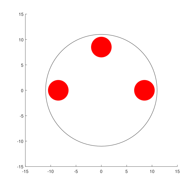
Figure 1: 3-Robot system work space schematic diagram.

5.1.2 Simulation Results

In the simulation, we set the sampling time $\Delta t=0.05$ s, $\rho=0.0001$ as the iterative algorithm design parameter, $P_{0}=P_{0}^{T}=100I_{36}>0$ and $\Theta_{0}=0_{36\times 18}$ as the initial values of the iterative algorithm. The initial value of the robot state vector $X(0)=z_{(1)}(0)=[x_{1}(0),y_{1}(0),\dots,x_{3}(0),y_{3}(0),v^{x}_{1}(0),v^{y}_{1}(0),\\ \dots,v^{x}_{3}(0),v^{y}_{3}(0)]^{T}=[-7,3,0,7,7,-4,0,0,0,0,0,0]^{T}$, which means Robot 1, Robot 2, and, Robot 3 are located at $(-7,3)$, $(0,7)$, $(7,-4)$ with zero initial speeds in X-direction and Y-direction at $k=0$. Correspondingly, the target positions of the three robots are $(-4.5,0)$, $(3,4)$, and $(3,-4)$. In $k_{s}=300$ iterations, apply a selected input vector $U(k)=[a_{1}^{x},a_{1}^{y},a_{2}^{x},a_{2}^{y},a_{3}^{x},a_{3}^{y}]^{T}$ (as shown in Table 1) to do the linear model approximation according to [8],[10].

Matrix $P(k)$ resetting. To improve the estimation results, we reset the matrix $P(k)=P_{0}$ every 130 iterations.

System Inputs
Input	Signal
$a_{1}^{x}$	$2\sin(0.075{k\pi})$
$a_{1}^{y}$	$3\cos(0.1833{k\pi})$
$a_{2}^{x}$	$3\sin(0.14{k\pi})$
$a_{2}^{y}$	$3\cos(0.095{k\pi})$
$a_{3}^{x}$	$-2\sin(0.06{k\pi})$
$a_{3}^{y}$	$-3\cos(0.092{k\pi})$

Table 1: Model identification system input components.

Parameter estimates. Figures 2-5 shows the results of parameter estimates.

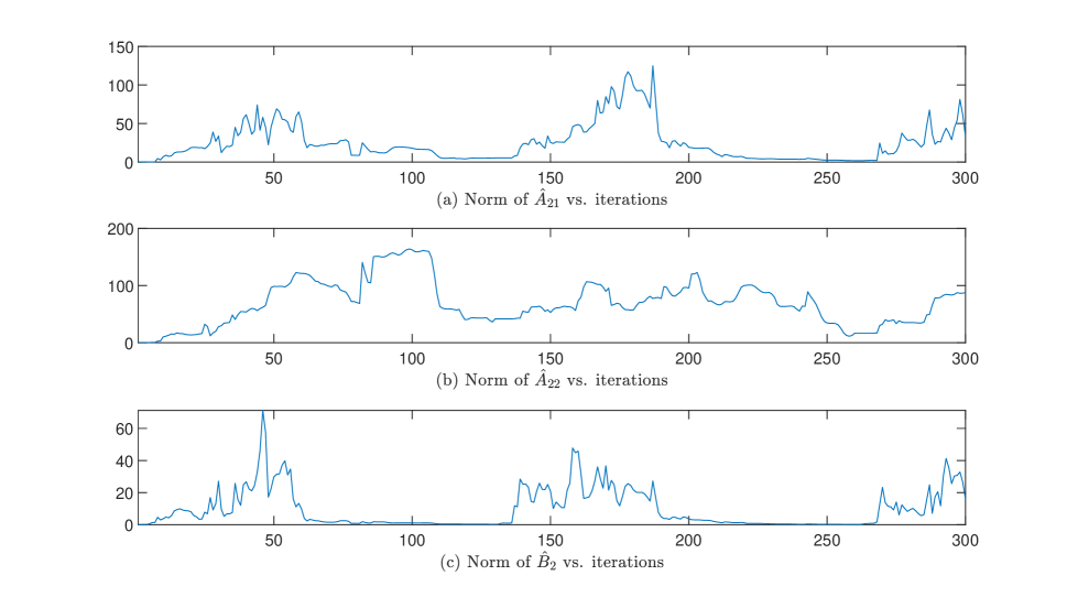
Figure 2: Norms of $\hat{\Theta}(k)$ (linear model identification for 3-robot system).

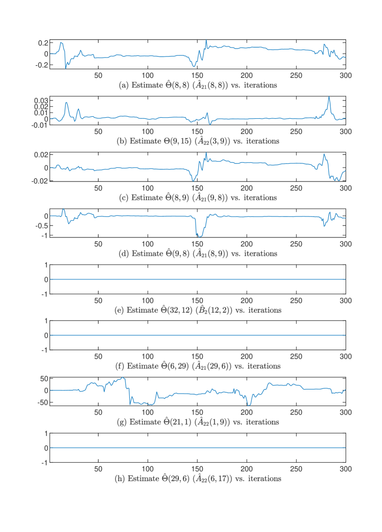
Figure 3: Components of $\hat{\Theta}(k)$ (linear model identification for 3-robot system).

Estimation errors. The results of the posteriori estimation error introduced in (5.8), $\epsilon_{a}(k)=\hat{\Theta}(k+1)\zeta(k)-z_{(2)}(k+1)$ are presented in Figure 4.

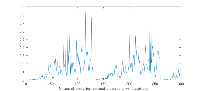
Figure 4: Norm of the posteriori estimation error $\epsilon_{a}(k)$ (linear model based).

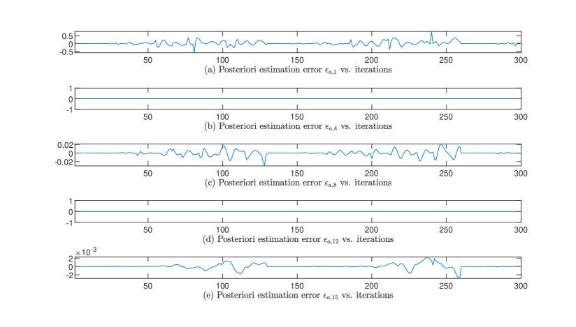
Figure 5: Components of the posteriori estimation error $\epsilon_{a}(k)$ (linear model based).

Discussion. The parameter matrix norms and some selected elements of the parameter matrix are demonstrated in Figures 2-5. The results of the posteriori estimation error introduced in (5.8), $\epsilon_{a}(k)=\hat{\Theta}(k+1)\zeta(k)-z_{(2)}(k+1)$ are presented in Figure 4. From Figures 4-7, we find that our iterative algorithm cannot estimate the parameters of the linear model well although both the posteriori estimation error norm and components are quite low. However, there is a non-ideal phenomenon in the simulation, the posteriori estimation error and the parameter estimates always have an obvious periodic increment tendency (from 0 to almost 0.9) during the iterations between two adjacent times we reset the parameter matrix $P$. This indicates that the estimated model cannot always ensure the estimation error within a small range, which may lead to undesired results while using the linear model based control signals.

Remark. In the above simulation, we also consider the distances between robots and the circular wall to check whether there are collisions happening. Since all the distances are larger than zero, no collisions happen during the identification process.

In [10], the linear model approximation simulation is implemented in a 5-robot system. According to the results, both the model validation error (the difference between the nonlinear utility component vector and the estimated output from the linear model with the fixed parameter matrix $\hat{\Theta}$ generated by several iterations of the adaptive parameter estimation algorithm) and the estimation error (the difference between the nonlinear utility component vector and the estimated output from the linear model with the online updating matrix $\hat{\Theta}(k)$ generated by minimizing the cost function $J_{3}$, defined in (3.1), of the adaptive parameter estimation algorithm) are quite low. However, tendencies of periodic increases in the estimation errors also appear in the 5-robot system simulation cases. This further proves the linear model may not be powerful to approximate the nonlinear utility functions and cannot be suitable to solve the optimal control problem.

5.2 Bilinear Model Identification of 3-robot System

In this subsection, the simulation system and the simulation results for the bilinear model identification of the 3-robot system are demonstrated sequentially. The estimation errors are examined to check the performance of the model (system) identification. The selected parameter components and the norms of the parameter matrices are analyzed for the parameter results.

5.2.1 Simulation System

The basic simulation construction and data collection logic are introduced in the following.

System state variables. System state variables $z(k)$ are constructed with natural state variables and utility function components. For the natural state variables $z_{(1)}(k)\in R^{12}$, the elements $z_{i}(k)$ are expressed as

$$z_{i}(k)=\psi_{i}(X(k))=X_{i}(k),\,i=1,2,\dots,12.$$ (5.9)

Utility functions components $z_{(2)}(k)\in R^{18}$ are expressed as

$$z_{(2)}=\psi_{(2)}(X(k))=[\psi_{13}(X(k)),\dots,\psi_{30}(X(k))]^{T}.$$ (5.10)

Bilinear model identification. To estimated the linear model of the nonlinear 3-robot system (2.66), as in (2.67)-(2.72), we have introduced

$$\hat{\Theta}(k)=[\hat{A}_{21}(k),\hat{A}_{22}(k),\hat{B}_{2}(k),\hat{f}(z_{(1)0},\,z_{(2)0}),\hat{\Phi}_{1}^{T}(k),\hat{\Phi}_{2}^{T}(k),\hat{\Phi}_{3}^{T}(k),\hat{\Phi}_{4}^{T}(k),\hat{\Phi}_{5}^{T}(k)]^{T}\in R^{901\times 18},$$ (5.11)

$$\zeta(k)=[(z_{(1)}(k)-z_{(1)0})^{T},(z_{(2)}(k)-z_{(2)0})^{T},U^{T}(k),1,g_{1}^{T}(\cdot),g_{2}^{T}(\cdot,\cdot),g_{3}^{T}(\cdot),g_{4}^{T}(\cdot,\cdot),g_{5}^{T}(\cdot,\cdot)]^{T}\in R^{901}.$$ (5.12)

The iterative algorithm for $\hat{\Theta}(k)=[\hat{\theta}_{1}(k),\hat{\theta}_{2}(k),\dots,\hat{\theta}_{18}(k)]\in R^{901\times 18}$ as the estimate of $\Theta$ in (2.70) has been given in (3.4)-(3.6).

Error signals. Similar to the linear model identification simulation, we also have two kinds of different error signals here:

• The estimation error $\epsilon(k)=\hat{\Theta}^{T}(k)\zeta(k)-z_{(2)}(k+1)$ is defined to estimate the unknown parameter matrix $\Theta$.

• The posteriori estimation error $\epsilon_{a}(k)=\hat{\Theta}^{T}(k+1)\zeta(k)-z_{(2)}(k+1)$ is defined to check the parameter estimation algorithm performance. The posteriori estimation error $\epsilon_{a}(k)$ is more meaningful for the algorithm performance because the parameter estimate $\hat{\Theta}(k)$ may not converge.

5.2.2 Simulation Results

In the simulation, we set the sampling time $\Delta t=0.05$ s, $\rho=0.0001$ as the iterative algorithm design parameter, $P_{0}=P_{0}^{T}=100I_{901}>0$ and $\Theta_{0}=0_{901\times 18}$ as the initial values of the iterative algorithm. The initial value of the robot state vector $X(0)=z_{(1)}(0)=[x_{1}(0),y_{1}(0),\dots,x_{3}(0),y_{3}(0),v^{x}_{1}(0),v^{y}_{1}(0),\\ \dots,v^{x}_{3}(0),v^{y}_{3}(0)]^{T}=[-7,3,0,7,7,-4,0,0,0,0,0,0]^{T}$, which means Robot 1, Robot 2, and, Robot 3 are located at $(-7,3)$, $(0,7)$, $(7,-4)$ with zero initial speeds in X-direction and Y-direction at $k=0$. Correspondingly, the target positions of the three robots are $(-4.5,0)$, $(3,4)$, and $(3,-4)$. In $k_{s}=300$ iterations, apply a selected input vector (as shown in Table 1) to do the linear model approximation with the simulation system introduced above.

Matrix $P(k)$ resetting. To improve the estimation results, we reset the matrix $P(k)=P_{0}$ every 75 iterations.

Parameter estimates. Figures 6-7 show the results of parameter estimates.

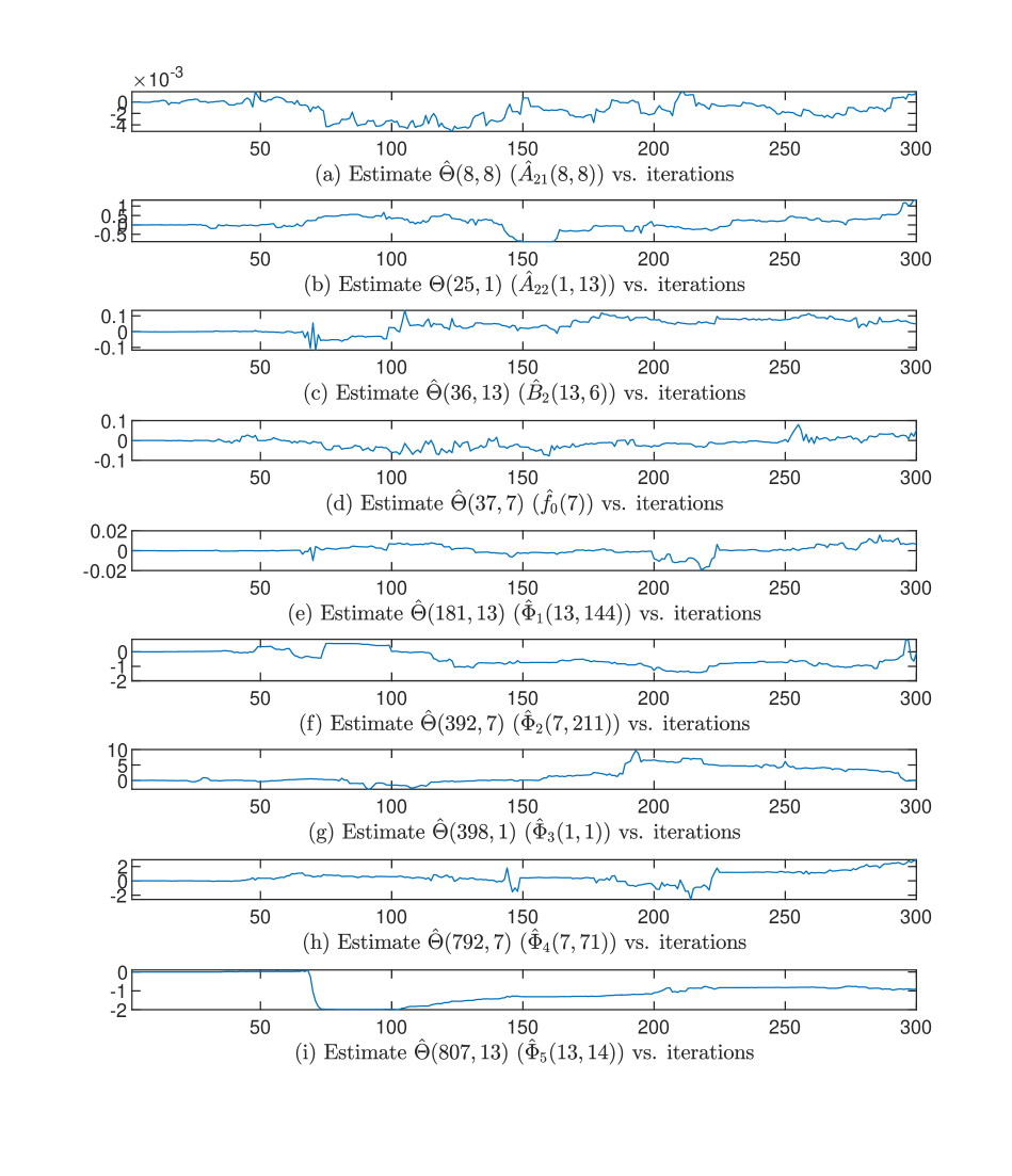
Figure 6: Components of $\hat{\Theta}(k)$ (bilinear model identification for 3-robot system).

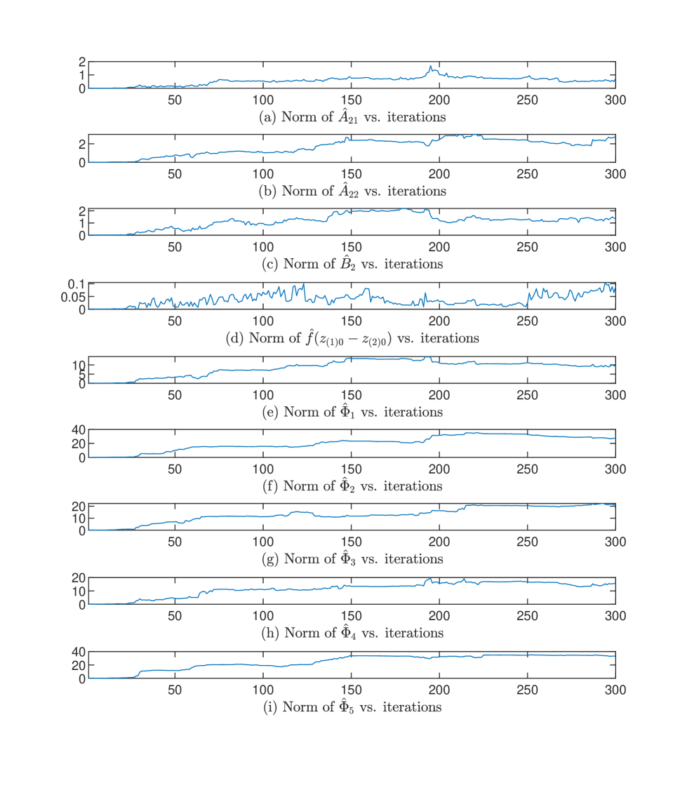
Figure 7: Norms of $\hat{\Theta}(k)$ (bilinear model identification for 3-robot system).

Estimation errors. The results of the posteriori estimation error introduced in (5.7), $\epsilon_{a}(k)=\hat{\Theta}(k+1)\zeta(k)-z_{(2)}(k+1)$ are presented in Figures 8-9.

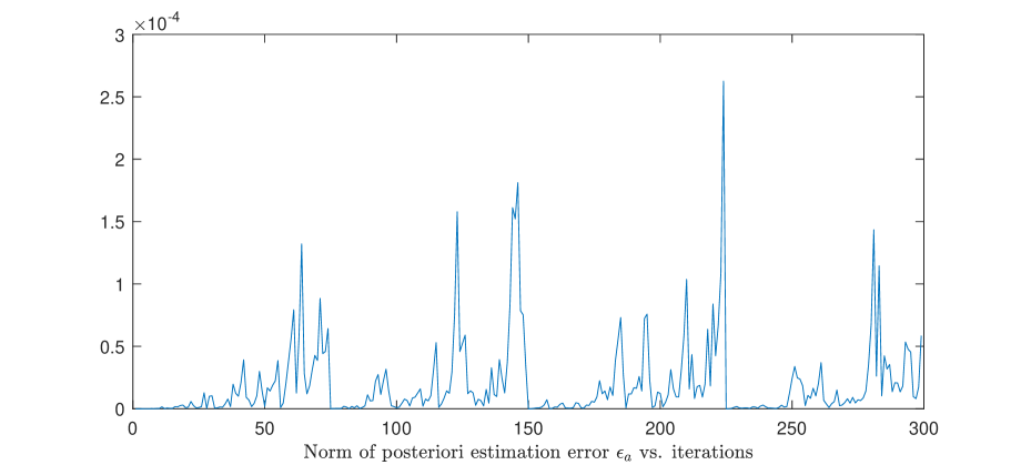
Figure 8: Norm of the posteriori estimation error $\epsilon_{a}(k)$ (bilinear model based).

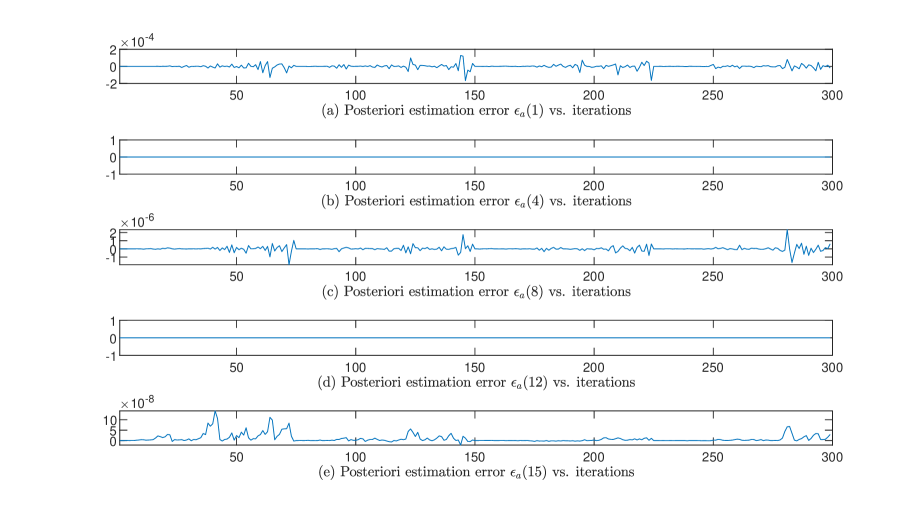
Figure 9: Components of the posteriori estimation error $\epsilon_{a}(k)$ (bilinear model based).

Remark. In the simulation, all the distances between robots and the circular wall are larger than zero, meaning no collisions happen between the robot and others or between the robot and the circular wall during this process.

Discussion. From Figures 8-9, we can find that our iterative algorithm can estimate the parameters of the bilinear model well since the norm of the posteriori estimation error $\epsilon_{a}(k)$ is always less than $3\times 10^{-4}$ and the components of the posteriori estimation error $\epsilon_{a}(k)$ are also quite small. Figures 6-7 indicate that all the parameter estimate norms and selected components change within a quite small range, although they do not converge. Thus, the bilinear model can better approximate the 3-robot system with the nonlinear utility functions since the posteriori estimation error of the bilinear model is much smaller than the posteriori estimation error of the linear model. Therefore, this bilinear model has a better performance to approximate the nonlinear utility functions although the tendency for periodic changes also appears in the corresponding results of the estimation error from the bilinear approximation model.

5.3 Linear and Bilinear Model Based Optimal Control for the 3-Robot System

In this subsection, the simulation system and the simulation results for evaluating the linear model based control design and the bilinear model based control design of the 3-robot system are demonstrated sequentially. The robot trajectories are presented to check whether the desired tracking objectives are achieved. During the feedback control phase, the distances between robots with others and robots with the wall are analyzed to check whether collisions happen.

5.3.1 Simulation Conditions

Before testing the performance of the proposed baseline control input, we need to use some iterations to estimate the linear approximation for the nonlinear model. Thus, there are two phases in the simulations for the baseline control input:

• Phase I (System Identification Phase): Initially, we set the sampling time $\Delta t=0.05$ s, $\rho=0.0001$ as the iterative algorithm design parameter, $P_{0}=P_{0}^{T}=100I_{a}>0$ and $\Theta_{0}=0_{a\times 18}$ as the initial values of the iterative algorithm. The initial value of the robot state vector $X(0)=z_{(1)}(0)=[x_{1}(0),y_{1}(0),\dots,x_{3}(0),y_{3}(0),v^{x}_{1}(0),v^{y}_{1}(0),\dots,v^{x}_{3}(0),v^{y}_{3}(0)]^{T}=[-7,3,0,7,7,-4,0,0,0,0,0,0]^{T}$, which means Robot 1, Robot 2, and, Robot 3 are located at $(-7,3)$, $(0,7)$, $(7,-4)$ with zero initial speeds in X-direction and Y-direction at $k=0$. Correspondingly, the target positions of the three robots are $(-4.5,0)$, $(3,4)$, and $(3,-4)$. In the first $k_{s}=300$ iterations, apply a selected proper input vector to do the linear or bilinear model approximation according to [8],[10]. The detailed steps for each system identification iteration are listed in the following:

  1. Compute the input $U(k)$, whose components are listed in Table 1.

  2. For the linear model identification, update the robots state $z_{(1)}(k)$ based on the robots dynamic equation (2.3). For the bilinear model identification, update the vector $z_{(1)}(k)-z_{(1)0}$ according to (2.3) and (2.47).

  3. For the linear model identification, calculate the utility components $z_{(2)}(k)$ based on equations (2.7)-(2.12) and (2.20). For the bilinear model identification, calculate the vector $z_{(2)}(k)-z_{(2)0}$ based on equations (2.7)-(2.12), (2.20) and (2.47).

  4. Update the approximations $\hat{z}_{(2)}(k+1)=\hat{\Theta}^{T}(k)\zeta(k)$, with $\hat{\Theta}^{T}(k)$, $\zeta(k)$ for the nonlinear utility functions based on equations (3.3)-(3.6). For the linear model identification, the signal vector $\zeta(k)$ and the parameter matrix $\hat{\Theta}(k)$ are defined in equations (2.40) and (2.43). Correspondingly, the the signal vector $\zeta(k)$ and the parameter matrix $\hat{\Theta}(k)$ of the bilinear model identification are defined in equations (2.68) and (2.71).

  Matrix $P(k)$ resetting. To improve the estimation results, we reset the matrix $P(k)=P_{0}$ every 130 iterations for linear model identification cases. Similarly, the matrix $P(k)$ is reset to be $P_{0}$ every 75 iterations in the bilinear model identification cases.

• Phase II (Feedback Control Phase): From the $(k_{s}+1)=301$th iteration, reset the initial and target positions of the robots and replace the input vector with the results of the linear programming problem to test the baseline control input performance and keep the updating of the model approximation results. Table 2 demonstrates the detailed robot initial and target position settings of the selected three cases. The details are listed in the following:

  1. Generate the input $U(k)$, which is the solution for the linear programming problem shown in equation (2.74) or (2.76).

  2. For the linear model identification, update the robots state $z_{(1)}(k)$ based on the robots dynamic equation (2.3). For the bilinear model identification, update the vector $z_{(1)}(k)-z_{(1)0}$ according to (2.3) and (2.47).

  3. For the linear model identification, calculate the utility components $z_{(2)}(k)$ based on equations (2.7)-(2.12) and (2.20). For the bilinear model identification, calculate the vector $z_{(2)}(k)-z_{(2)0}$ based on equations (2.7)-(2.12), (2.20) and (2.47).

  4. Update the approximations $\hat{z}_{(2)}(k+1)=\hat{\Theta}^{T}(k)\zeta(k)$, with $\hat{\Theta}^{T}(k)$, $\zeta(k)$ for the nonlinear utility functions based on equations (3.3)-(3.6). For the linear model identification, the signal vector $\zeta(k)$ and the parameter matrix $\hat{\Theta}(k)$ are defined in equations (2.40) and (2.43). Correspondingly, the the signal vector $\zeta(k)$ and the parameter matrix $\hat{\Theta}(k)$ of the bilinear model identification are defined in equations (2.68) and (2.71).

  Case Settings
  Case number	Robot number	Initial position	Target position
  Case I	Robot 1	$(-4.48,3.3)$	$(-4.5,0)$
  	Robot 2	$(2.98,7.11)$	$(3,4)$
  	Robot 3	$(3.65,-5.70)$	$(3,-4)$
  Case II	Robot 1	$(-3.1,3.3)$	$(-3,0.5)$
  	Robot 2	$(4.9,4.6)$	$(5,2)$
  	Robot 3	$(0.9,-5)$	$(0.5,-3.5)$
  Case III	Robot 1	$(7.5,2.5)$	$(7.5,0)$
  	Robot 2	$(-5.1,-2.5)$	$(-5,-5)$
  	Robot 3	$(-5.2,3.5)$	$(-5,5)$
  Case IV	Robot 1	$(-3.1,-0.6)$	$(-3.5,-3.5)$
  	Robot 2	$(0,2.5)$	$(0.2,0)$
  	Robot 3	$(4.8,3)$	$(5.3,5)$
  Case V	Robot 1	$(-6.4,5.3)$	$(-6,2.4)$
  	Robot 2	$(-2.5,1.8)$	$(-2.5,-1.4)$
  	Robot 3	$(3,-2.7)$	$(2.5,-1.4)$

  Table 2: Settings of the feedback control phase.

5.3.2 Simulation Results

The linear model based control design and the bilinear based control design simulation results are presented in Figure 10. The plot of the robot trajectories controlled by the linear model based control design during the corresponding control evaluation phase is shown in Figure 10(a). Then, Figures 10(b)-10(f) show the robot trajectories controlled by the bilinear model based control design during the control evaluation phase in all five cases.

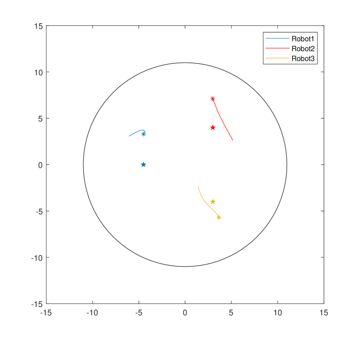
(a) Case I (linear model based control design)

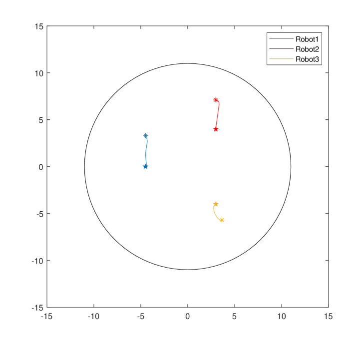
(b) Case I (bilinear model based control design)

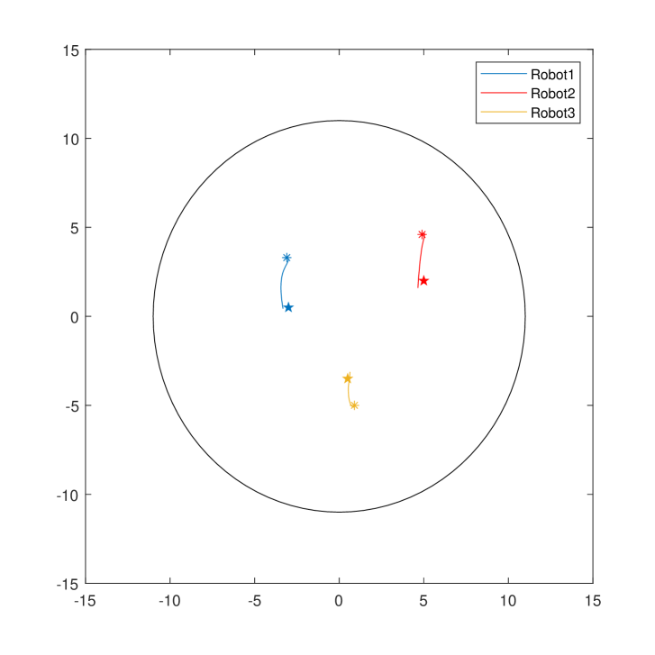
(c) Case II (bilinear model based control design)

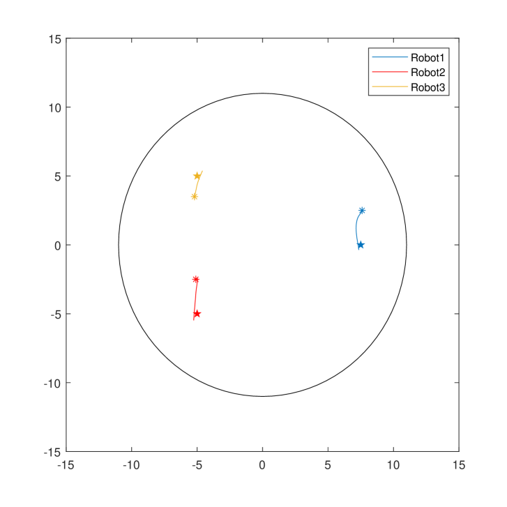
(d) Case III (bilinear model based control design)

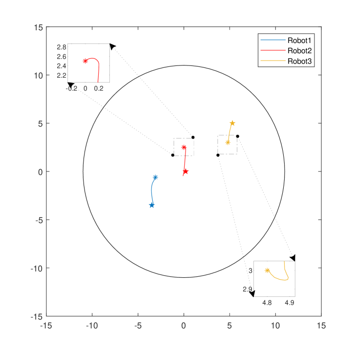
(e) Case IV (bilinear model based control design)

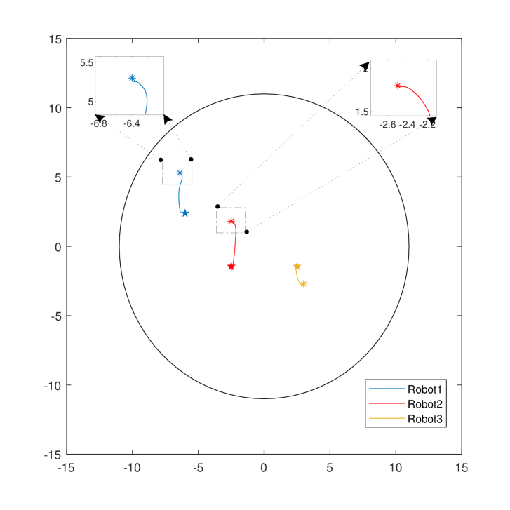
(f) Case V (bilinear model based control design)

The asterisk markers $*$ in different colors indicate the initial positions of the robots, and the five-point-star markers $\star$ represent the target positions of the robots. The lines in different colors are the trajectories of the robots and the big black circle is the circular wall of the workspace for the robots.

Figure 10: Robot trajectories in different cases.

Remark. According to the analysis of the distances between the robots and the circular wall in all cases, the control evaluation is collision-free since all the distances are larger than zero indicating that the robots do not collide with others or with the wall in all five cases.

Discussion. From Figure 10, only the bilinear model based control design can achieve the control objective to make all the robots arrive at their targets without collisions. According to Figure 10(a), only Robot3 passes by the vicinal positions of its corresponding target. The other two robots cannot move toward the desired positions. Thus, although the linear model based control can achieve part of the control objective, a more elaborate approximation model should be considered to achieve the control objective.

Figures 10(b)-10(f) demonstrate the robots can reach the corresponding targets (or vicinal positions) simultaneously controlled by the baseline control input based on the estimated bilinear model for the $3-$robot system with the nonlinear utility functions in all five cases. This proves that the proposed optimal design based on the bilinear approximation model for the multi-robot system with the nonlinear utility functions can achieve the control objective which is reaching the target positions and collision-free.

Additionally, in Figure 10(e), the blue robot (Robot$1$) moves down to its left initially. The red robot (Robot$2$) moves toward our right-hand side direction at first. Then, it moves downward. The yellow robot (Robot$3$) also moves towards our right-hand side at first. This happens because the three robots interact with each other to avoid possible collisions since their initial distances are too short. Similarly, in Figure 10(f), we can see that both the blue robot (Robot$1$) and the red robot (Robot$2$) do not move directly toward their targets. Instead, the blue robot (Robot$1$) moves away from the wall (the lower right direction of their initial direction) at first to avoid the possible collision between itself and the wall. At the same time, the red robot (Robot$2$) moves toward our right-hand side at first to keep a safe distance from the approaching Robot$1$. The reason for this phenomenon is that the initial distance between the blue robot and the red robot and the initial distance between the blue robot and the wall are too close. These two cases show that the algorithm can make robots interact with each other to avoid possible collisions.

For the bilinear model based optimal control simulations of the selected five cases, the control evaluation phase lasts 30 iterations, which indicates 1.5 seconds in the actual situation based on the sampling time $\Delta t=0.05$ seconds. The simulation program for the control evaluation phase costs 1.30 seconds for Case 1, 1.29 seconds for Case 2, 1.31 seconds for Case 3, 1.35 seconds for Case 4, and 1.33 seconds for Case 5 based on i7-8700k CPU. Thus, the ability of the control algorithm to solve the real problem is further proved. However, this control algorithm may not be global. In some cases, the robots’ initial positions are far away from their targets, the robots cannot reach the target positions (or vicinal target positions).

5.4 Simulations Results of Decentralized Control

In this subsection, the simulation system and the simulation results for evaluating the bilinear model based decentralized control design of the 3-robot system are demonstrated sequentially. The robot trajectories are presented to check whether the desired tracking objectives are achieved. During the feedback control phase, the distances between robots with others and robots with the wall are analyzed to check whether collisions happen.

5.4.1 Simulation Conditions

Similar to previous simulations, the simulation of the decentralized cases includes two phases too:

• Phase I (System Identification Phase): Initially, we set the sampling time $\Delta t=0.05$s, $\rho=0.0001$ as the iterative algorithm design parameter, $P_{i}(-1)=P_{i}^{T}(-1)=100I_{109}>0,i=1,2,3$ and $\Theta_{i}(0)=0_{109\times 6}$ as the initial values of the iterative algorithm for every single robot. The initial value of the robot state vectors are defined as $z_{(1),1}(0)=[x_{1}(0),y_{1}(0),v^{x}_{1}(0),v^{y}_{1}(0)]^{T}=[-8.5,-1,0,0]^{T}$, $z_{(1),2}(0)=[x_{2}(0),y_{2}(0),v^{x}_{2}(0),v^{y}_{2}(0)]^{T}=[0,8.5,\\ 0,0]^{T}$, $z_{(1),3}(0)=[x_{3}(0),y_{3}(0),v^{x}_{3}(0),v^{y}_{3}(0)]^{T}=[8.5,0,0,0]^{T}$ which means Robot 1, Robot 2, and Robot 3 are located at $(-8.5,-1)$, $(0,8.5)$, and $(8.5,0)$ with zero initial speeds in X-direction and Y-direction at $k=0$. Correspondingly, the target positions of the three robots are $(-6.5,0)$, $(0,6.5)$, and $(6.5,0)$. In the first $k_{s}=300$ iterations, apply a selected proper input vector to do the linear or bilinear model approximation according to [8],[10]. The detailed steps for each system identification iteration are listed in the following:

  1. Compute the input $U_{i}(k)$, whose components are listed in Table 1.

  2. Update all the vectors for every robot $z_{(1),i}(k),i=1,2,3$, according to (4.11).

  3. Calculate all the vectors for every robot $z_{(2),i}(k),i=1,2,3$, based on equation (4.12).

  4. Update the approximations for each robot $\hat{z}_{(2),i}(k+1)=\hat{\Theta}_{i}^{T}(k)\zeta_{i}(k),i=1,2,3$, with $\hat{\Theta}^{T}_{i}(k)$, $\zeta_{i}(k)$ for the nonlinear utility functions based on equations (3.3)-(3.6). The signal vector $\zeta_{i}(k)$ and the parameter matrix $\hat{\Theta}_{i}(k)$ are defined in equations (4.20) and (4.23).

• Phase II (Feedback Control Phase): From the $(k_{s}+1)=301$th iteration, reset the initial and target positions of the robots and replace the input vector with the results of the linear programming problem to test the baseline control input performance and keep the updating of the model approximation results. Table 3 demonstrates the detailed robot initial and target position settings of the selected two cases. The details are listed in the following:

  1. Generate the input $U_{i}(k)$, which is the solution for the linear programming problem shown in equation (4.26).

  2. Update all the vectors for every robot $z_{(1),i}(k),i=1,2,3$, according to (4.11).

  3. Calculate all the vectors for every robot $z_{(2),i}(k),i=1,2,3$, based on equation (4.12).

  4. Update the approximations for each robot $\hat{z}_{(2),i}(k+1)=\hat{\Theta}_{i}^{T}(k)\zeta_{i}(k),i=1,2,3$, with $\hat{\Theta}^{T}_{i}(k)$, $\zeta_{i}(k)$ for the nonlinear utility functions based on equations (3.3)-(3.6). The signal vector $\zeta_{i}(k)$ and the parameter matrix $\hat{\Theta}_{i}(k)$ are defined in equations (4.20) and (4.23).

  Case Settings
  Case number	Robot number	Initial position	Target position
  Case I	Robot 1	$(-2.5,7.1)$	$(-3.5,5)$
  	Robot 2	$(2.7,3.3)$	$(3.5,5)$
  	Robot 3	$(-0.8,-3.5)$	$(0,-5.5)$
  Case II	Robot 1	$(-6.5,-2.9)$	$(-4.5,0)$
  	Robot 2	$(1.7,2.3)$	$(3,4)$
  	Robot 3	$(2.4,-5.2)$	$(3,-4)$

  Table 3: Settings of the feedback control phase.

5.4.2 Simulation Results

The bilinear based decentralized control design simulation results are presented in Figure 11.

Model identification results. The results of the model identification phases are almost the same as the results in Section 5.2. The posteriori estimation error in the case applying the decentralized bilinear model identification algorithm is always small without any periodical changes.

Optimal control results. In Figure 11, (a)-(b) demonstrate the robots can reach the corresponding targets (or vicinal positions) simultaneously controlled by the decentralized generated control input based on the estimated bilinear model for the 3 robot system with the nonlinear utility functions in both cases. This proves that the decentralized version optimal design based on the bilinear approximation model for the multi-robot system with the nonlinear utility functions can achieve the control objective which is reaching the target positions and collision-free.

For the simulations of the selected two cases, the control evaluation phase lasts 30 iterations, which indicates 1.5 seconds in the actual situation based on the sampling time $\Delta t=0.05$ seconds. The simulation program of the control evaluation phase for the three robots costs 1.73 seconds for Case I, and 1.71 seconds for Case II based on i7-8700k CPU. Since the control inputs for each robot are generated decentralized, we can use three computers to find the optimal control input simultaneously. Thus, the running time of the control evaluation phase for every single robot can be decreased to one-third of the listed running time for all three robots. This proves that not only the decentralized bilinear model based control design is fast enough to be implemented for real-time control, but also that the algorithm can be accelerated by applying its decentralized version with more computation resources.

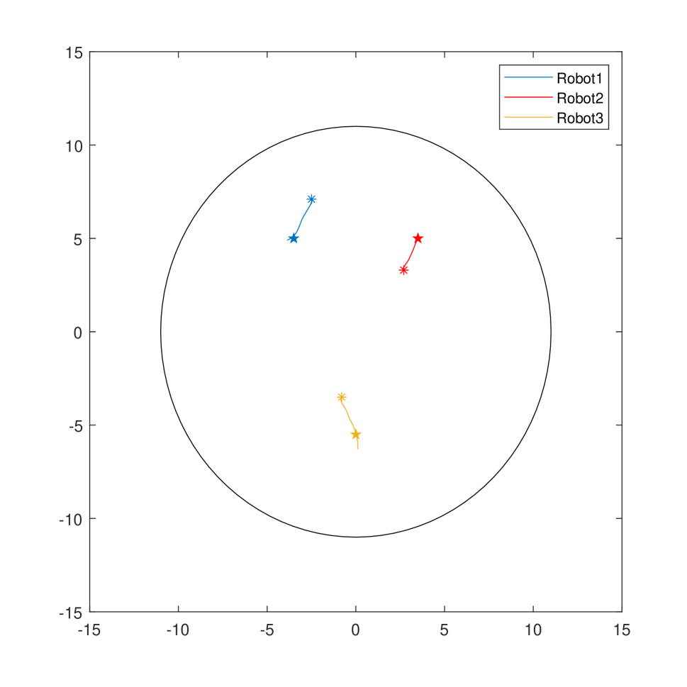
(a) Case I

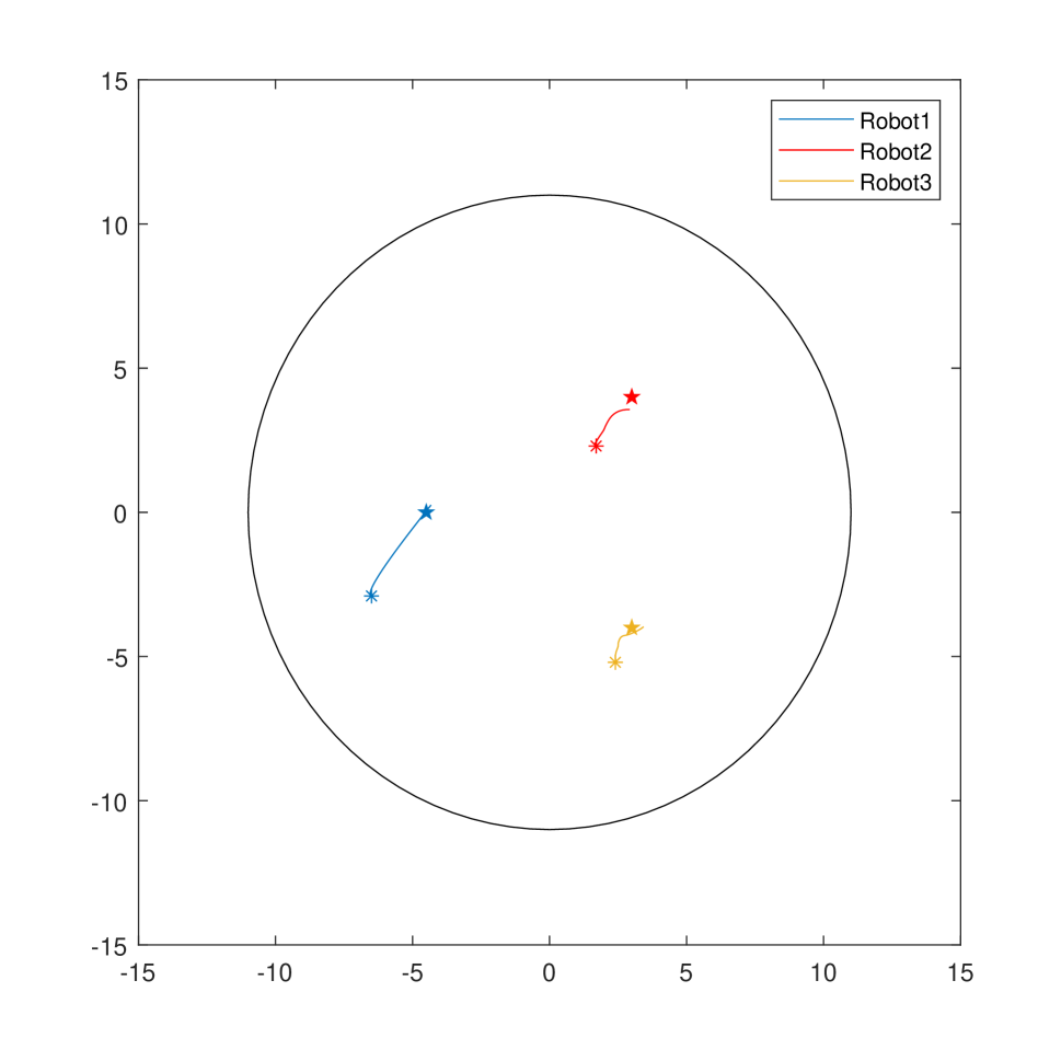
(b) Case II

The asterisk markers $*$ in different colors indicate the initial positions of the robots, and the five-point-star markers $\star$ represent the target positions of the robots. The lines in different colors are the trajectories of the robots and the big black circle is the circular wall of the workspace for the robots.

Figure 11: Robot trajectories in different cases (Bilinear model based decentralized control).

5.5 Additional Parameter Estimation Algorithm: Normalized Adaptive Gradient Algorithm

The least-squares algorithm (3.4)-(3.6) has a big matrix $P(k)$ to calculate. We also simulated the cases that applied another parameter estimation algorithm called the normalized adaptive gradient algorithm to see whether it can make the results better.

With the same definition of the estimation error $\epsilon(k)=\hat{\Theta}^{T}(k)\zeta(k)-y(k)$ as the least squares algorithm and the measured vector signals $y(k)\in R^{18}$ and $\zeta(k)\in R^{q}$ , the adaptive law of the gradient algorithm is defined as

$$\hat{\Theta}(k+1)=\hat{\Theta}(k)-\frac{\Gamma\zeta(k)\epsilon^{T}(k)}{m^{2}(k)},k=k_{0},\,k_{0}+1,\,k_{0}+2,\cdots,$$ (5.13)

where $0<\Gamma=\Gamma^{T}<2I_{q}$ , and

$$m(k)=\sqrt{\rho+\zeta^{T}(k)\zeta(k)},\,\rho>0.$$ (5.14)

5.5.1 Simulation Results

In the simulation, We replace the least squares parameter estimation algorithm of Step 4 in both of the system identification phase and the feedback control phase of the bilinear model based control evaluation simulation procedures in Section 5.3 with the gradient algorithm.

With the application of the gradient algorithm as parameter estimation method, the robot trajectories in the simulation results for all the cases in Section 5.3 show the robots cannot reach their targets. Although different values of $\Gamma$ lead to different trajectories, most trajectories are even almost straight lines without any collision avoidance behaviors or moving direction adjustment toward the corresponding target behaviors.

6 Concluding Remarks

In this report, we have finished the simulation studies of the Koopman system approximation based optimal control of multiple robots with nonlinear utility functions, which is detailed in [11]. The desired robot tracking performance is ensured by maximizing the nonlinear utility function. In [11], an algorithm to find the linear or bilinear approximations of the nonlinear utility function components and the optimal control design based on the estimated linear or bilinear approximations. In this report, the simulation results of the linear or bilinear approximation algorithm and the control designs based on the approximations are reported and analyzed.

Specifically, we formulate a 3-robot system to examine the performance of the control designs based on the linear approximation model and bilinear approximation model. According to the linear and bilinear model identification simulation results in Section 5.1-5.2, only the centralized bilinear model can approximate the nonlinear utility functions well since only the bilinear model identification can ensure the posteriori estimation error within a smaller range, i.e. $|\epsilon_{a}|=(0,3\times 10^{-4})$. Simulation results in Section 5.3 show that the centralized linear model based control design can only achieve parts of the tracking objectives, which means the linear model does not contain rich enough information to construct the optimal control design. After that, other results in Section 5.3 prove that the centralized bilinear model based optimal control design can achieve the desired tracking objectives in all three listed cases under the computation time restriction for the real-time control. Lastly, Section 5.4 shows the decentralized bilinear model based control signals can also achieve the desired tracking objectives faster. The success of the simulation for the decentralized bilinear model based control inputs infers the proposed bilinear model based optimal control algorithm owns the potential to be applied to more complex applications, like autonomous driving.

In the future, the performance of the bilinear model based optimal control design can be improved to ensure the desired global tracking performance within a shorter computation time.

References

- [1] G. Tao, Adaptive Control Design and Analysis, John Wiley & Sons, Hoboken, NJ, 2003.
- [2] M. O. Williams, I. G. Kevrekidis, and C. W. Rowley, “A data–driven approximation of the Koopman operator: extending dynamic mode decomposition,” Journal of Nonlinear Science, vol. 25, pp. 1307–1346, 2015.
- [3] M. Korda and I. Mezic, “Linear predictors for nonlinear dynamical systems: Koopman operator meets model predictive control,” Automatica, vol. 93, no. 7, pp. 149-160, July 2018.
- [4] E. Yeung, S. Kundu, and N. O. Hodas, “Learning deep neural network representations for Koopman operators of nonlinear dynamical systems,” Proceedings of 2019 American Control Conference, pp. 4832-4839, 2019.
- [5] J. Wang, Q. Dai, D. Shen, X. Song, X. Chen, S. Huang, and D. Filev, “Multi-agent navigation with collision avoidance: game theory approach,” Ford Report 2020-X, October 2020.
- [6] P. Bevanda, S. Sosmowski, and S. Hirche, “Koopman operator dynamical models: learning, analysis and control,” arXiv:2102.02522 [eess.SY], 2021 (https://arxiv.org/abs/2102.02522).
- [7] M. Mazouchi, S. Nageshrao, and H. Modares, “Finite-time Koopman identifier: a unified batch-online learning framework for joint learning of Koopman structure and parameters,” arXiv:2105.05903 [eess.SY], 2021 (https://arxiv.org/abs/2105.05903).
- [8] G. Tao, “Koopman transformations for nonlinear dynamic systems,” Ford URP Report 2021-6, December 2021.
- [9] G. Tao, “Linear control formulation for multi-robot systems with nonlinear utility function,” Ford URP Report 2022-2, March 2022.
- [10] Q. H. Zhao and G. Tao, “Simulation study of linear model approximation for a 5-robot system with nonlinear utility functions,” Ford URP Report 2022-1, January 2021.
- [11] G. Tao and Q. H. Zhao, “Koopman system approximation based optimal control of multiple robots—Part I: concepts and formulations,” Manuscript 2023-05-01, May 2023 (submitted to arXiv).