Improved Logical Reasoning of Language Models via Differentiable Symbolic Programming

Abstract

Pre-trained large language models (LMs) struggle to perform logical reasoning reliably despite advances in scale and compositionality. In this work, we tackle this challenge through the lens of symbolic programming. We propose DSR-LM, a Differentiable Symbolic Reasoning framework where pre-trained LMs govern the perception of factual knowledge, and a symbolic module performs deductive reasoning. In contrast to works that rely on hand-crafted logic rules, our differentiable symbolic reasoning framework efficiently learns weighted rules and applies semantic loss to further improve LMs. DSR-LM is scalable, interpretable, and allows easy integration of prior knowledge, thereby supporting extensive symbolic programming to robustly derive a logical conclusion. The results of our experiments suggest that DSR-LM improves the logical reasoning abilities of pre-trained language models, resulting in a significant increase in accuracy of over 20% on deductive reasoning benchmarks. Furthermore, DSR-LM outperforms a variety of competitive baselines when faced with systematic changes in sequence length.

1 Introduction

Complex applications in natural language processing involve dealing with two separate challenges. On one hand, there is the richness, nuances, and extensive vocabulary of natural language. On the other hand, one needs logical connectives, long reasoning chains, and domain-specific knowledge to draw logical conclusions. The systems handling these two challenges are complementary to each other and are likened to psychologist Daniel Kahneman’s human “system 1” and “system 2” Kahneman (2011): while the former makes fast and intuitive decisions, akin to neural networks, the latter thinks more rigorously and methodically. Considering LMs as “system 1” and symbolic reasoners as “system 2”, we summarize their respective advantages in Table 1.

Although pre-trained LMs have demonstrated remarkable predictive performance, making them an effective “system 1”, they fall short when asked to perform consistent logical reasoning (Kassner et al., 2020; Helwe et al., 2021; Creswell et al., 2022), which usually requires “system 2”. In part, this is because LMs largely lack capabilities of systematic generalization (Elazar et al., 2021; Hase et al., 2021; Valmeekam et al., 2022).

Language Model	Symbolic Reasoner
• Rapid reasoning • Sub-symbolic knowledge • Handling noise, ambiguities, and naturalness • Process open domain text • Can learn in-context	• Multi-hop reasoning • Compositionality • Interpretability • Data efficiency • Can incorporate domain-specific knowledge

Table 1: Respective advantages of language models and symbolic reasoners.

In this work, we seek to incorporate deductive logical reasoning with LMs. Our approach has the same key objectives as neuro-symbolic programming (Chaudhuri et al., 2021): compositionality, consistency, interpretability, and easy integration of prior knowledge. We present DSR-LM, which tightly integrates a differentiable symbolic reasoning module with pre-trained LMs in an end-to-end fashion. With DSR-LM, the underlying LMs govern the perception of natural language and are fine-tuned to extract relational triplets with only weak supervision. To overcome a common limitation of symbolic reasoning systems, the reliance on human-crafted logic rules (Huang et al., 2021; Nye et al., 2021), we adapt DSR-LM to induce and fine-tune rules automatically. Further, DSR-LM  allows incorporation of semantic loss obtained by logical integrity constraints given as prior knowledge, which substantially helps the robustness.

We conduct extensive experiments showing that DSR-LM can consistently improve the logical reasoning capability upon pre-trained LMs. Even if DSR-LM uses a RoBERTa backbone with much less parameters and does not explicitly take triplets as supervision, it can still outperform various baselines by large margins. Moreover, we show that DSR-LM can induce logic rules that are amenable to human understanding to explain decisions given only higher-order predicates. As generalization over long-range dependencies is a significant weakness of transformer-based language models (Lake and Baroni, 2018; Tay et al., 2020), we highlight that in systematic, long-context scenarios, where most pre-trained or neural approaches fail to generalize compositionally, DSR-LM can still achieve considerable performance gains.

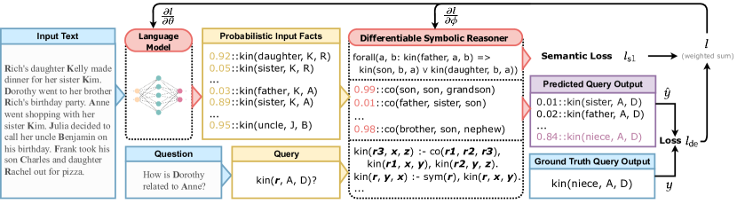
Figure 1: Overview of DSR-LM with a motivating example where “Anne is the niece of Dorothy” should be logically inferred from the context. We abbreviate the names with their first initials in the relational symbols.

2 Related Work

Logical reasoning with LMs. Pre-trained LMs have been shown to struggle with logical reasoning over factual knowledge (Kassner et al., 2020; Helwe et al., 2021; Talmor et al., 2020a). There is encouraging recent progress in using transformers for reasoning tasks (Zhou et al., 2020; Clark et al., 2021; Wei et al., 2022; Chowdhery et al., 2022; Zelikman et al., 2022) but these approaches usually require a significant amount of computation for re-training or human annotations on reasoning provenance (Camburu et al., 2018; Zhou et al., 2020; Nye et al., 2021; Wei et al., 2022). Moreover, their entangled nature with natural language makes it fundamentally hard to achieve robust inference over factual knowledge (Greff et al., 2020; Saparov and He, 2022; Zhang et al., 2022).

There are other obvious remedies for LMs’ poor reasoning capability. Ensuring that the training corpus contains a sufficient amount of exemplary episodes of sound reasoning reduces the dependency on normative biases and annotation artifacts (Talmor et al., 2020b; Betz et al., 2020; Hase et al., 2021). Heuristics like data augmentation are also shown to be effective (Talmor et al., 2020b). But the above works require significant efforts for crowdsourcing and auditing training data. Our method handily encodes a few prototypes/templates of logic rules and is thus more efficient in terms of human effort. Moreover, our goal is fundamentally different from theirs in investigating the tight integration of neural and symbolic models in an end-to-end manner.

Neuro-symbolic reasoning. Neuro-symbolic approaches are proposed to integrate the perception of deep neural components and the reasoning of symbolic components. Representative works can be briefly categorized into regularization (Xu et al., 2018), program synthesis (Mao et al., 2018), and proof-guided probabilistic programming (Evans and Grefenstette, 2018; Rocktäschel and Riedel, 2017; Manhaeve et al., 2018; Zhang et al., 2019; Huang et al., 2021). To improve compositionality of LMs, previous works propose to parameterize grammatical rules (Kim, 2021; Shaw et al., 2021) but show that those hybrid models are inefficient and usually underperform neural counterparts. In contrast to the above works, DSR-LM focuses on improving LMs’ reasoning over logical propositions with tight integration of their pre-trained knowledge in a scalable and automated way.

3 Methodology

3.1 Problem Formulation

Each question answering (QA) example in the dataset is a triplet containing input text $x$, query $q$, and the answer $y$. Figure 1 shows an instance that we will use as our running example. The input text $x$ is a natural language passage within which there will be a set of entities, possibly referenced by 3rd person pronouns. The sentences hint at the relationships between entities. For example, “Dorothy went to her brother Rich’s birthday party” implies that Rich is Dorothy’s brother and Dorothy is Rich’s sister. The query $q$ is a tuple of two entities, representing the people with whom we want to infer the relation. The expected relation is stored in the answer $y$, which will be one of a confined set of possible relations $\mathcal{R}$, allowing us to treat the whole problem as an $|\mathcal{R}|$-way classification problem. We focus only on the problems where the desired relation is not explicitly stated in the context but need to be deduced through a sequence of reasoning.

3.2 Methodology Overview

The design of DSR-LM concerns tightly integrating a perceptive model for relation extraction with a symbolic engine for logical reasoning. While we apply LMs for low-level perception and relation extraction, we employ a symbolic reasoning module to consistently and logically reason about the extracted relations. With a recent surge in neuro-symbolic methods, reasoning engines are made differentiable, allowing us to differentiate through the logical reasoning process. In particular, we employ Scallop Huang et al. (2021) as our reasoning engine. We propose two add-ons to the existing neuro-symbolic methodology. First, some rules used for logical deduction are initialized using language models and further tuned by our end-to-end pipeline, alleviating human efforts. Secondly, we employ integrity constraints on the extracted relation graphs and the logical rules, to improve the logical consistency of LMs and the learned rules.

Based on this design, we formalize our method as follows. We adopt pretrained LMs to build relation extractors, denoted $\mathcal{M}_{\theta}$, which take in the natural language input $x$ and return a set of probabilistic relational symbols $\mathbf{r}$. Next, we employ a differentiable deductive reasoning program, $\mathcal{P}_{\phi}$, where $\phi$ represents the weights of the learned logic rules. It takes as input the probabilistic relational symbols and the query $q$ and returns a distribution over $\mathcal{R}$ as the output $\hat{y}$. Overall, the deductive model is written as

$$\hat{y}=\mathcal{P}_{\phi}(\mathcal{M}_{\theta}(x),q).$$ (1)

Additionally, we have the semantic loss (sl) derived by another symbolic program $\mathcal{P}_{\texttt{sl}}$ computing the probability of violating the integrity constraints:

$$l_{\texttt{sl}}=\mathcal{P}_{\texttt{sl}}(\mathcal{M}_{\theta}(x),\phi)$$ (2)

Combined, we aim to minimize the objective $J$ over training set $\mathcal{D}$ with loss function $\mathcal{L}$:

$$J(\theta,\phi) =\frac{1}{|\mathcal{D}|}\sum_{(x,q,y)\in\mathcal{D}}w_{1}\mathcal{L}(\mathcal{P}_{\phi}(\mathcal{M}_{\theta}(x),q),y)$$ (3)

$$+w_{2}\mathcal{P}_{\texttt{sl}}(\mathcal{M}_{\theta}(x),\phi),$$

where $w_{1}$ and $w_{2}$ are tunable hyper-parameters to balance the deduction loss and semantic loss.

3.3 Relation Extraction

Since pre-trained LMs have strong pattern recognition capabilities for tasks like Named-Entity-Recognition (NER) and Relation Extraction (RE) (Tenney et al., 2019; Soares et al., 2019), we adopt them as our neural components in DSR-LM. To ensure that LMs take in strings of similar length, we divide the whole context into multiple windows. The goal is to extract the relations between every pair of entities in each windowed context. Concretely, our relation extractor $\mathcal{M}_{\theta}$ comprises three components: 1) a Named-Entity Recognizer (NER) to obtain the entities in the input text, 2) a pre-trained language model, to be fine-tuned, that converts windowed text into embeddings, and 3) a classifier that takes in the embedding of entities and predicts the relationship between them. The set of parameters $\theta$ contains the parameters of both the LM and the classifier.

We assume the relations to be classified come from a finite set of relations $\mathcal{R}$. For example in CLUTRR (Sinha et al., 2019), we have 20 kinship relations including mother, son, uncle, father-in-law, etc. In practice, we perform $(|\mathcal{R}|+1)$-way classification over each pair of entities, where the extra class stands for “n/a”. The windowed contexts are split based on simple heuristics of “contiguous one to three sentences that contain at least two entities”, to account for coreference resolution. The windowed contexts can be overlapping and we allow the reasoning module to deal with noisy and redundant data. Overall, assuming that there are $m$ windows in the context $x$, we extract $mn(n-1)(|\mathcal{R}|+1)$ probabilistic relational symbols. Each symbol is denoted as an atom of the form $p(s,o)$, where $p\in\mathcal{R}\cup\{\text{n/a}\}$ is the relational predicate, and $s$, $o$ are the two entities connected by the predicate. We denote the probability of such symbol extracted by the LM and relational classifier as $\Pr(p(s,o)~{}|~{}\theta)$. All these probabilities combined form the output vector $\mathbf{r}=\mathcal{M}_{\theta}(x)\in\mathbb{R}^{mn(n-1)(|\mathcal{R}|+1)}$.

3.4 Differentiable Symbolic Inference

The symbolic inference modules $\mathcal{P}_{\phi}$ and $\mathcal{P}_{\texttt{sl}}$ are responsible for processing the extracted relations to deduce 1) an expected output relation in $\mathcal{R}$, and 2) a semantic loss encoding the probability of constraint violation. There are two main objectives for these modules. First, they need to logically reason about the output relation and the semantic loss based on the extracted relational symbols $\mathbf{r}$, the query $q$, and the rule weights $\phi$. Second, they need to compute the gradients of $\hat{y}$ and $l_{\texttt{sl}}$ with respect to $\theta$ and $\phi$, namely $\frac{\partial\hat{y}}{\partial\theta}$, $\frac{\partial\hat{y}}{\partial\phi}$, $\frac{\partial l_{\texttt{sl}}}{\partial\phi}$, and $\frac{\partial l_{\texttt{sl}}}{\partial\theta}$, in order for the fine-tuning and rule learning to happen.

Logical deduction.

Logic rules can be applied to known facts to deduce new ones. For example, below is a horn clause, which reads “if $b$ is $a$’s brother and $c$ is $b$’s daughter, then $c$ is $a$’s niece”:

$$\text{niece}(a,c)~{}\leftarrow~{}\text{brother}(a,b)\wedge\text{daughter}(b,c).$$

Note that the structure of the above rule can be captured by a higher-order logical predicate called “composite” (abbreviated as ). This allows us to express many other similarly structured rules with ease. For instance, we can have and . With this set of rules, we may derive more facts based on known kinship relations. In fact, composition is the only kind of rule we need for kinship reasoning. In general, there are many other useful higher-order predicates to reason over knowledge bases, which we list out in Table 2.

Predicate	Example
transitive	$\text{transitive}(\text{relative})$
symmetric	$\text{symmetric}(\text{spouse})$
inverse	$\text{inverse}(\text{husband},\text{wife})$
implies	$\text{implies}(\text{mother},\text{parent})$

Table 2: Higher-order predicate examples.

Probability propagation.

We seek to have the deduced facts to also be associated with probabilities computed using probabilities predicted by the underlying relation extractor $\mathcal{M}_{\theta}$. This is achieved by allowing the propagation of probabilities. For example, we have the proof tree with probabilities:

In practice, there could be multiple steps in the proof tree (multi-hop) and one fact can be derived by multiple proof trees. We employ the inference algorithms based on approximated weighted model counting (WMC) presented in Manhaeve et al. (2018) to account for probabilistic inference under complex scenarios. Since the WMC procedure is augmented for differentiation, we can obtain the gradient $\frac{\partial\hat{y}}{\partial\mathbf{r}}$. From here, we can obtain $\frac{\partial\hat{y}}{\partial\theta}=\frac{\partial\hat{y}}{\partial\mathbf{r}}\frac{\partial\mathbf{r}}{\partial\theta}$, where the second part can be automatically derived from differentiating $\mathcal{M}_{\theta}$.

Rule learning.

Hand-crafted rules could be expensive or even impossible to obtain. To alleviate this issue, DSR-LM applies LMs to help automatically extract rules, and further utilizes the differentiable pipeline to fine-tune the rules. Each rule such as is attached a weight, initialized by prompting an underlying LM. For example, the prompt we use for extracting is “one’s $r$’s $p$ is their <$q$:mask>”. Given that the relations $r,p,q\in\mathcal{R}$, DSR-LM  automatically enumerates $r$ and $p$ from $\mathcal{R}$ while querying for LM to unmask the value of $q$. LM then returns a distribution of words, which we take an intersection with $\mathcal{R}$. The probabilities combined form the initial rule weights $\phi$. This type of rule extraction strategy is different from existing approaches in inductive logic programming since we are exploiting LMs for existing knowledge about relationships.

Note that LMs often make simple mistakes answering such prompt. In fact, with the above prompt, even GPT-3 can only produce 62% of composition rules correctly. While we can edit prompt to include few-shot examples, in this work we consider fine-tuning such rule weights $\phi$ within our differentiable reasoning pipeline. The gradient with respect to $\phi$ is also derived with the WMC procedure, giving us $\frac{\partial\hat{y}}{\partial\phi}$. In practice, we use two optimizers with different hyper-parameters to update the rule weights $\phi$ and the underlying model parameter $\theta$, in order to account for optimizing different types of weights.

Semantic loss and integrity constraints.

In general, learning with weak supervision label is hard, not to mention that the deductive rules are learnt as well. We thereby introduce an additional semantic loss during training. Here, semantic loss is derived by a set of integrity constraints used to regularize the predicted entity-relation graph as well as the learnt logic rules. In particular, we consider rules that detect violations of integrity constraints. For example, “if A is B’s father, then B should be A’s son or daughter” is an integrity constraint for relation extractor—if the model predicts a father relationship between A and B, then it should also predict a son or daughter relationship between B and A. Encoded in first order logic, it is

$$\forall a,b,\text{father}(a,b)\Rightarrow(\text{son}(b,a)\vee\text{daughter}(b,a)).$$

Through differentiable reasoning, we evaluate the probability of such constraint being violated, yielding our expected semantic loss. In practice, arbitrary number of constraints can be included, though too many interleaving ones could hinder learning.

⬇

// Relation declaration

type kinship(rela: String, subject: String, object: String)

type query(subject: String, object: String)

type composite(r1: String, r2: String, r3: String)

// Rules to derive the final answer

rel kinship(r3,a,c) = kinship(r1,a,b), kinship(r2,b,c), composite(r1,r2,r3), a != c

rel answer(r) = query(s, o), derive(r, s, o)

// Integrity constraints (6 for kinship graph and 2 for rule learning)

rel violation(!r) = r := forall(a, b: kinship(FATHER, a, b) =>

kinship(SON, b, a) or kinship(DAUGHTER, b, a)) // Other constraints are omitted...

Figure 2: The Scallop program used in the CLUTRR reasoning task.

4 Experiments

We evaluate DSR-LM on both CLUTRR and DBpedia-INF. We show that DSR-LM has accurate and generalizable long-range reasoning capability.

4.1 Datasets

CLUTRR (Sinha et al., 2019) consists of kinship reasoning questions. Given a context that describes a family’s routine activity, the goal is to deduce the relationship between two family members that is not explicitly mentioned in the story. Although the dataset is synthetic, the sentences are crowd-sourced and hence there is a considerable amount of naturalness inside the dataset. The family kinship graph is synthetic and the names of the family members are randomized. For ablation study, we manually crafted 92 kinship composition rules as an external symbolic knowledge base. This yields the following symbolic information for each datapoint: 1) the full kinship graph corresponding to the story, 2) the symbolic knowledge base (KB), and 3) a query representing the question. The CLUTRR dataset is divided into different difficulties measured by $k$, the number of facts used in the reasoning chain. For training, we only have 10K data points with 5K $k=2$ and another 5K $k=3$, meaning that we can only receive supervision on data with short reasoning chains. The test set, on the other hand, contains 1.1K examples with $k\in\{2,\dots,10\}$.

DBpedia-INF is a curated subset of the evaluation dataset used in RuleBert Saeed et al. (2021). Similar to CLUTRR, it is generated synthetically to test the reasoning capability of LMs. Given a synthetic passage describing the relation between entities, and soft deductive logic rules, we aim to deduce the relationship between any two entities. The symbolic program of DBpedia-INF consists of 26 predicates, 161 soft rules mined from DBpedia, and 16 rules defining the negation and symmetricity between the predicates. The difficulty of the questions is represented in terms of reasoning length from $k\in\{0,\dots,5\}$. Larger $k$ implies harder question. Compared to the exact dataset used in Rulebert, we clean it in order to ensure the question-answer pairs are logically consistent and probabilistically correct.

4.2 Experimental Setup

Implementation.

We employ Scallop Huang et al. (2021) as the differentiable symbolic inference module. We show the program used for CLUTRR reasoning task in Figure 2. It comprises relation type declarations, deductive rules for kinship reasoning, and integrity constraints for computing semantic loss (attached in the Appendix). The program used for DBpedia-INF is written in a similar manner with additional high-order predicates listed in Table 2.

Pre-trained LMs for fine-tuning.

We used the HuggingFace (Wolf et al., 2019) pre-trained w2v-google-news-300, RoBERTa-base, and DeBERTa-base as the pretrained language models. We finetune RoBERTa-base and DeBERTa-base during training with binary cross entropy loss. Our relation extraction module is implemented by adding an MLP classifier after the LM, accepting a concatenation of the embedding of the two entities and the embedding of the whole windowed context.

Our model.

Our main model, DSR-LM, uses RoBERTa as the underlying LM. The relation classifier is a 2-layer fully connected MLP. For training, we initialize $\phi$ by prompting the LM. To accelerate the learning process, we use multinomial sampling to retrieve 150 rules for symbolic reasoning. During testing, we will instead pick the top 150 rules. We use two Adam optimizer to update $\theta$ and $\phi$, with learning rate $10^{-5}$ and $10^{-2}$ respectively.

For ablation studies, we present a few other models. First, we ablate on back-bone LMs. Specifically, we have DSR-LM-DeBERTa which uses DeBERTa as the back-bone LM. DSR-w2v-BiLSTM, on the other hand, uses as back-bone the word2vec Mikolov et al. (2013) model for word embedding and BiLSTM Huang et al. (2015) for sequential encoding. For DSR-LM-with-Manual-Rule we treat the logic rules as given, meaning that we provide 92 composition rules for CLUTRR and around 180 rules for DBpedia-INF. In this case, we set ground truth rules to have $1.0$ weight and therefore $\phi$ is not learnt. Then, we have DSR-LM-without-IC which does not have integrity constraints and semantic loss. Lastly, we have DSR-without-LM that takes ground truth structured entity relation graph as input. This way, we do not need the underlying relation extractor and only $\phi$ needs to be learned.

Baselines.

We compare DSR-LM with a spectrum of baselines from purely neural to logically structured. The baselines include pretrained large language models (BERT (Kenton and Toutanova, 2019) and RoBERTa (Liu et al., 2019)), non-LM counterparts (BiLSTM (Hochreiter and Schmidhuber, 1997; Cho et al., 2014) and BERT-LSTM), structured models (GAT (Veličković et al., 2018), RN (Santoro et al., 2017), and MAC (Hudson and Manning, 2018)), and other neuro-symbolic models (CTP Minervini et al. (2020), RuleBert (Saeed et al., 2021)). The structured models include those models with relational inductive biases, while the neuro-symbolic model uses logic constraints.

Baseline setup.

We highlight a few baselines we include for completeness but are treated as unfair comparison to us: GAT, CTP, and GPT-3 variants. All baselines other than GAT and CTP take as input natural language stories and the question to produce the corresponding answer. GAT and CTP, on the contrary, takes entity relation graph rather than natural language during training and testing.

The model sizes are different across baselines as well. Model size generally depends on two parts, the backbone pre-trained LM, and the classification network built upon the LM. GPT-3 contains 175B parameters, and RoBERTa uses 123M parameters. The classification model of our method has 2.97M parameters (assuming using embeddings from RoBERTa). With extra 10K parameters for rule weights, our DSR-LM framework has around 127M parameters.

For GPT-3 variants, we conduct experiments on CLUTRR with GPT-3 under the Zero-Shot (GPT-3 ZS), GPT-3 Fine-Tuned (GPT-3 FT), and Few(5)-Shot (GPT-3 5S) (Brown et al., 2020), as well as Zero-Shot-CoT (GPT-3 ZS-CoT) (Kojima et al., 2022a) settings. For fair comparison, we also include the ground truth kinship composition knowledge in GPT-3 zero shot (GPT-3 ZS w/ Rule), and 5 shot (GPT-3 5S w/ Rule). We include the prompts we used and additional details in Appendix A.

Figure 3: DSR-LM’s performance on CLUTRR compared with various baselines

Test Length	DSR-LM	RuleBert
Overall	95.87	72.59
0	100.0	98.40
1	100.0	54.80
2	98.4	75.20
3	89.2	64.00
4	88.1	69.89
5	100.0	72.29

Table 3: DBpedia-INF generalization evaluation under different test reasoning length. Models are trained on 10K reasoning length $k=0$ sequences, and tested on sequences of reasoning length $k=[0,5]$.

Confidence	Learnt Rules
1.154	mother($a$,$c$) $\leftarrow$ sister($a$,$b$) $\wedge$ mother($b$,$c$)
1.152	daughter($a$,$c$) $\leftarrow$ daughter($a$,$b$) $\wedge$ sister($b$,$c$)
1.125	sister($a$,$c$) $\leftarrow$ daughter($a$,$b$) $\wedge$ aunt($b$,$c$)
1.125	father($a$,$c$) $\leftarrow$ brother($a$,$b$) $\wedge$ father($b$,$c$)
1.123	granddaughter($a$,$c$) $\leftarrow$ grandson($a$,$b$) $\wedge$ sister($b$,$c$)
1.120	brother($a$,$c$) $\leftarrow$ sister($a$,$b$) $\wedge$ brother($b$,$c$)
1.117	brother($a$,$c$) $\leftarrow$ son($a$,$b$) $\wedge$ uncle($b$,$c$)
1.105	brother($a$,$c$) $\leftarrow$ daughter($a$,$b$) $\wedge$ uncle($b$,$c$)
1.104	daughter($a$,$c$) $\leftarrow$ wife($a$,$b$) $\wedge$ daughter($b$,$c$)
1.102	mother($a$,$c$) $\leftarrow$ brother($a$,$b$) $\wedge$ mother($b$,$c$)
$\dots$	$\dots$

Table 4: The learnt top-10 confident logic rules over CLUTRR.

(a) Comparison to common baselines

(b) Comparison to GPT-3 related baselines

Figure 4: Systematic generalization performance comparison on CLUTRR dataset. Models except GPT-3-ZS*, GPT-3-FS are trained (or fine-tuned) on $k\in\{2,3\}$. All models are tested on $k\in\{2,\dots,10\}$.

4.3 Experimental Results

DSR-LM  systematically outperforms a wide range of baselines by a large margin.

We evaluate DSR-LM and baselines on both CLUTRR and DBpedia-INF, as reported in Figure 3 and Table 3.

In the CLUTRR experiment, DSR-LM achieves the best performance among all the models (Figure 3). Next, we examine how models trained on stories generated from clauses of length $k\leq 3$ and evaluated on stories generated from larger clauses of length $k\geq 4$. A fine-grained generalizability study reveals that although all models’ performances decline as the reasoning length of the test sequence increases, pure neural-based models decrease the fastest (Figure 4(a) and 4(b)). It manifests the systematic issue that language models alone are still not robust for length generalization (Lake and Baroni, 2018). On the other hand, the performance of DSR-LM decreases much slower as test reasoning length increases and outperforms all the baselines when $k\geq 4$.

In the DBpedia-INF experiment, DSR-LM outperforms RuleBert by 37% in terms of overall performance (Table 3), showing that DSR-LM has much more robust generalization. Recall that RuleBert aims to improve the logical reasoning of LMs by straightforward fine-tuning with soft rules and facts. Our results show that augmenting data alone for fine-tuning do not effectively improve systematicity. Meanwhile, DSR-LM  imbues reasoning inductive biases throughout training and learns useful rules to generalize to longer reasoning lengths.

Learning interpretable logic rules.

DSR-LM  is capable of producing explicit logic rules as part of the learning process. For presentation, we show the top-10 rules learnt from DSR-LM model in Table 4. We compare the top-92 most likely prompted and fine-tuned rules against the 92 hand-crafted rules, and 70 of them match. Additionally, we find that our rule weight fine-tuning helps correct 11 of the incorrect rules produced by LM. Through this qualitative analysis, it is clear that DSR-LM provides an interface to probe and interpret the intermediate steps, enhancing the interpretability.

GPT-3 variants are inferior in long-range reasoning.

Interestingly, ZS scores 28.6% accuracy on CLUTRR while ZS-CoT scores 25.6%, suggesting that the chain-of-thought prompting might not work in long-range reasoning (Figure 3). In fact, there are many cases where GPT-3 favors complication over simplicity: GPT-3 frequently answers “stepdaughter”, “stepmother”, and “adopted son”, while the real answers are simply “daughter”, “mother”, and “son”. Additionally, GPT-3 could derive the correct result for the wrong reason, e.g. “Jeffrey is Gabrielle’s son, which would make William her grandson, and Jeffrey’s brother.” While we count the final answer to be correct (William is Jeffrey’s brother), there is a clear inconsistency in the reasoning chain: William cannot be Gabrielle’s grandson and Jeffrey’s brother simultaneously, given that Jeffrey is Gabrielle’s son. Lastly, we observe that, both GPT-3 FT and many other methods have an accuracy drop as $k$ becomes larger (Figure 4(b)), ZS and ZS-CoT stay relatively consistent, suggesting that the size of context and the reasoning chain may have a low impact on GPT-3’s performance.

4.4 Analyses and Ablation Studies

Symbolic reasoner consistently improves LMs and word embeddings.

Since DSR-LM has a model agnostic architecture, we study how the choice of different LMs impacts the reasoning performance. As shown in Table 5, the two transformer-based models have on-par performance and outperform the word2vec one. However, note that the word2vec-based model still has better performance than all other baselines. Besides higher final accuracy, the pre-trained transformer-based language model also accelerates the training process. Both DSR-LM-RoBERTa and DSR-LM-DeBERTa reach their best performance within 20 epochs, while it takes DSR-w2v-BiLSTM 40 epochs to peak.

Model	Accuracy (%)
DSR-LM (RoBERTa)	60.98 $\pm$ 2.64
DSR-LM-DeBERTa	60.92 $\pm$ 2.72
DSR-w2v-BiLSTM	40.39 $\pm$ 0.06

Table 5: Ablation study about neural backbones of DSR-LM. We compare the CLUTRR performance of DSR-LM using different LMs.

Incorporate domain knowledge.

DSR-LM allows injecting domain specific knowledge. In DSR-LM-with-Rule, we manually crafted 92 rules for kinship reasoning to replace the learnt rules. As shown in Table 6, it obtained a 0.36% performance gain over DSR-LM. The fact that the improvement is marginal implies our method extracts useful rules to obtain on-par performance with manually crafted ones. DSR-LM-without-IC, our model without integrity constraints specified on predicted relations and rules, performs worse than DSR-LM, suggesting that logical integrity constraints are essential component for improving the model robustness.

Model	Accuracy (%)
DSR-LM	60.98 $\pm$ 2.64
DSR-LM-without-IC	51.48 $\pm$ 0.57
DSR-LM-with-Manual-Rule	61.34 $\pm$ 1.56

Table 6: Ablation study. We compare our model’s performance on CLUTRR with different setups.

The impact of the relation extractor.

To understand what causes the failure case of DSR-LM, we study the performance of our relation classification model separately. We isolate the trained relation extractor and found that it reaches 84.69% accuracy on the single relation classification task. For comparison, we train a relation extractor using all the intermediate labels in the training dataset, and it reaches 85.32% accuracy. It shows that even using only weak supervision (i.e., the final answers to multi-hop questions), our approach can reach on-par performance as supervised relation extraction.

Reasoning over structured KBs.

To understand the rule learning capability of our approach, we design our ablation model DSR-without-LM to take as input ground-truth KBs instead of natural language. In this case, rule weights are not initialized by LM but randomized. As shown in Table 7, our model outperforms GAT and CTP which also operates on structured KBs. It demonstrates that our differentiable rule learning paradigm learns rules to reason about KBs consistently.

Model	Accuracy (%)
GAT	39.05
CTP	95.57
DSR-without-LM	98.81

Table 7: DSR-without-LM compared against GAT and CTP on reasoning with ground truth KBs. For this comparison we train on $k\in[2,3]$ and test on $k\in[4,10]$.

Failure cases of DSR-LM.

We showcase in Appendix Table 8 that even state-of-the-art large LMs are prone to logical fallacies. On the other hand, the failure case of our method usually occurs in the stage of relation extraction. For example, for the following sentence “Christopher and Guillermina are having a father-daughter dance”, our RoBERTa based relation extractor fails to recognize the father-daughter relationship but rather thinks C and G have a husband-wife relationship. We require most of the relation extraction to be correct in order to avoid cascading error. As the error rate on individual relation extraction accumulates, it leads to the observed drop in accuracy as $k$ becomes larger.

5 Concluding Remarks

We investigate how to improve LMs’ logical reasoning capability using differentiable symbolic reasoning. Through extensive experiments, we demonstrate the effectiveness of DSR-LM over challenging scenarios where widely deployed large LMs fail to reason reliably. We hope our work can lay the groundwork for exploring neuro-symbolic programming techniques to improve the robustness of LMs on reasoning problems.

Appendix A Implementation Details

Hardware. We perform all the experiments on a server with two 20-core Intel Xeon CPUs, four GeForce RTX 2080 Ti GPUs, and 768 GB RAM.

Reasoner details. The learning of rules and the fine-tuning of the underlying LM should happen separately with different learning rates – fine-tuning LM is an intricate process that requires a very small learning rate, while rules should be learned with larger learning rates since gradients are directly back-propagated onto the weights. This can be realized by employing two separate optimizers, one for fine-tuning and the other for rule learning. During training time, we rotate training the two parts by toggling one and the other optimizer for every 10 batches of data points.

Rule learning training setup. For rule learning, we can initialize the transitivity tensor using the language model provided composite rules. Since the CLUTRR dataset consists of $20$ different relations and a transitivity relationship is defined over $3$ relations, there are 8K possible transitivity facts over these relations. Specifically, we give every predicted composite rule by the GPT with a $0.5$ weight, while initializing the other rules with a range such as $[0,0.1]$, since otherwise, an insensible transitive fact may be getting a random high weight while it effectively does nothing for reasoning. The learning process encourages the rules that yield the correct query result and suppresses the rules that lead to wrong answers. To avoid the exponential blow-up caused by injecting all the 8K rules in the reasoning engine, we sample $200$ rules according to their weights during the training time and deterministically use the top $200$ learned rules during the test time. For the QA-No-Rule setup, the confidence score of rules, the MLP classifier for relation extraction, and the underlying LM are learned and updated simultaneously during training. To account for their difference, we employ two Adam optimizers $A_{\text{RL}}$ and $A_{\text{RE}}$. $A_{\text{RE}}$ is used for optimizing models for relation extraction, and thus will take as parameters the MLP classifier and the underlying LM. It has a low learning rate $0.00001$ since it needs to fine-tune LMs. $A_{\text{RL}}$, on the other hand, will take as a parameter the confidence score tensor for the transitive rules, and is set to have a higher learning rate of $0.001$. For the integrity constraints, we set the result integrity violation loss with the weight $0.1$, and set the rule integrity constraint violation loss with the weight $0.01$. We set the batch size to $16$ and train for $20$ epochs.

To obtain the initial rule weights for the composition rule in our CLUTRR experiment, the prompt we use is “Mary’s P’s Q is her <mask>.” where P and Q are enumerations of all possible relationships, and the unmasked value is treated as the answer R, producing composite(P, Q, R). For the other rule templates we used, the prompts are

1. transitive: “is R’s R one’s R? <mask>”; the probability of the unmasked word being “yes” is treated the rule weight for transitive(R).

2. symmetric: “does A is R of B means B is R of A? <mask>”; the probability of the unmasked word being “yes” is treated the rule weight for symmetric(R).

3. inverse: “A is R of B means B is <mask> of A”; the unmasked value is treated as the answer P, producing inverse(R, P).

4. implies: “does R imply P? <mask>”; the probability of unmasked value being “yes” is treated as the rule weight for implies(R, P).

GPT-3 Prompt Setups. For Zero-Shot, we use the prompt “So $B$ is $A$’s:” for the query pair $(A,B)$ to ask GPT-3 to complete the relationship between $A$ and $B$. We pick the phrase in the first line or before the first period from the completed text and compare it directly with the ground truth relation. For the Few(5)-Shot setting, we randomly select 5 examples from the training dataset used for other models ($k\in[2,3]$) to serve as examples. We use the same prompt for Few-Shot and Fine-Tuned as the Zero-Shot and the automated GPT-3 fine-tuning setup for our training dataset, trained for 4 epochs. To add in the transitive KB, we simply include 92 hand-crafted rules in natural language as a part of the prompt, and we performed Zero-shot with KB, and Few(5)-shot with KB experiments. For the Zero-Shot-CoT setting, we use the prompt “Who is $B$ to $A$? Let’s think step by step” to suggest GPT-3 to auto-complete while working out a reasoning chain. Under this setup, it is impossible to compare the answer to the ground truth automatically. Therefore, we manually check through the whole test dataset of CLUTRR.

Appendix B Additional Experimental Results

In Table 8, we showcase the failure cases of large LMs for logical inference, where Zero-shot-CoT denotes zero-shot chain-of-thoughts (Kojima et al., 2022b).

$k$ Prompt GPT-3 CoT Output Ground Truth 2 Jeffrey asked his brother William if he would come help him fix his car next weekend. Gabrielle was delighted to see her grandson, William, at her birthday party. Who is Jeffrey to Gabrielle? Let’s do it step by step: Jeffrey is Gabrielle’s grandson. William is Jeffrey’s brother. grandson 3 Elliott felt lonely when his wife Marian was gone to see her mother Molly. Elliott and his daughter Karen took a day off school to go to the zoo. Who is Karen to Molly? Let’s do it step by step: Karen is Elliott’s daughter. Molly is Elliott’s wife’s mother. Therefore, Karen is Molly’s granddaughter. granddaughter 4 Frank took his daughter Julia to the park. Beverly, Emilie´s sister went with them. Kimberley was excited because today she was going to the zoo with her uncle Frank. Jenny spent a great day shopping with her daughter, Kimberley. Who is Beverly to Jenny? Let’s do it step by step: Beverly is Jenny’s sister-in-law. niece 5 Melissa and her father, Stephen, went to the marina. Stephen’s daughter, Margaret, had purchased a boat, and they were eager to see it. Annie and her aunt, Evelyn, went to the deli. They got a half a pound of corned beef, and two pounds of salami. Melissa and her sister Annie were arguing over a toy. While they were fighting, Melissa’s sister Margaret grabbed the toy, and ran off to play with it by herself. Who is Evelyn to Melissa? Let’s do it step by step: Melissa’s father is Stephen. Stephen has a daughter, Margaret. Margaret is Annie’s aunt. Therefore, Evelyn is Annie’s aunt, and Melissa’s great-aunt. aunt 6 James took his grandson Davis to the baseball game. Sharon and her son Brian went out to lunch together yesterday. Brian and his brother Oliver went to the park to play basketball. Davis played scrabble with his mother Sharon and his brother Oliver. Davis asked his brother Oliver if he would come help him fix his car next weekend. Who is James to Oliver? Let’s do it step by step: James is Davis’s grandfather, so he is Oliver’s great-grandfather. grandfather 7 George rushed to the hospital to find out that his wife and already given birth to a boy and had named him David. Larry was playing checkers with his brother Craig. Larry’s sister Jean was waiting to play. Judy made mixed drinks for her son Craig. Judy’s daughter Jean was jealous because she was n’t offered one. Jean planned a trip to the zoo for her brother, Craig. They had a great time. George was having trouble with his divorce because he only got to see his daughter Jean a few times a week. Who is David to Craig? Let’s do it step by step: George’s wife gave birth to a boy and named him David. David is Craig’s nephew. brother 8 Anthony went to the bakery with his uncle Roger to pick up some bread for lunch. Anthony loved going to the store with his mom Mary. She always bought him snacks Charles would n’t let his son Floyd go to the park by himself. Floyd’s brother Anthony offered to go with him. Faye was hoping to travel out of state to visit her son Cecil. Ellie’s brother, Charles, was doing his best to find the best flight. Mary and her son Anthony went out to lunch together yesterday. Cecil took her sister, Christine, out to dinner for her birthday. Who is Roger to Christine? Let’s do it step by step: Cecil is Faye’s son, so Faye is Christine’s mother-in-law. Christine is married to Faye’s son, so Christine is Faye’s daughter-in-law. Charles is Ellie’s brother, so Charles is Christine’s brother-in-law. Anthony is Charles’s son, so Anthony is Christine’s nephew. Roger is Anthony’s uncle, so Roger is Christine’s brother-in-law. uncle 9 Gino bought gifts for his lovely sister, Jami. Michele and William left that evening to go bowling. Ethel and her son, Gordon, went to the park, and had a wonderful time. Manuel’s father, Kenneth, thought his son was a monster. Meanwhile Michele thought her son Manuel was a little angel. Gino, Kenneth’s other son, agreed with his dad. William asked his brother Larry if he would come help him fix his car next weekend. Joseph was so happy for his brother, Larry, getting a promotion. Gordon and his uncle Joseph went to the movies Sunday after church and got popcorn and candy while they were there. Who is Jami to Ethel? Let’s do it step by step: 1. Jami is Gino’s sister. 2. Ethel is Gino’s mother. 3. Therefore, Jami is Ethel’s daughter-in-law. niece

Table 8: Qualitative analysis of GPT-3 Zero-Shot-CoT on the CLUTRR dataset. The novelty comes from the sentence marked in orange. Queries that are of interest are marked in blue. Correct answer in the output is marked green and incorrect ones are marked red.

Confidence Rule 1.154 mother(A,B) $\leftarrow$ sister(A,C) $\wedge$ mother(C,B) 1.152 daughter(A,B) $\leftarrow$ daughter(A,C) $\wedge$ sister(C,B) 1.125 sister(A,B) $\leftarrow$ daughter(A,C) $\wedge$ aunt(C,B) 1.125 father(A,B) $\leftarrow$ brother(A,C) $\wedge$ father(C,B) 1.123 granddaughter(A,B) $\leftarrow$ grandson(A,C) $\wedge$ sister(C,B) 1.120 brother(A,B) $\leftarrow$ sister(A,C) $\wedge$ brother(C,B) 1.117 brother(A,B) $\leftarrow$ son(A,C) $\wedge$ uncle(C,B) 1.105 brother(A,B) $\leftarrow$ daughter(A,C) $\wedge$ uncle(C,B) 1.104 daughter(A,B) $\leftarrow$ wife(A,C) $\wedge$ daughter(C,B) 1.102 mother(A,B) $\leftarrow$ brother(A,C) $\wedge$ mother(C,B) 1.102 brother(A,B) $\leftarrow$ father(A,C) $\wedge$ son(C,B) 1.096 sister(A,B) $\leftarrow$ mother(A,C) $\wedge$ daughter(C,B) 1.071 sister(A,B) $\leftarrow$ father(A,C) $\wedge$ daughter(C,B) 1.071 son(A,B) $\leftarrow$ son(A,C) $\wedge$ brother(C,B) 1.070 uncle(A,B) $\leftarrow$ father(A,C) $\wedge$ brother(C,B) 1.066 daughter(A,B) $\leftarrow$ son(A,C) $\wedge$ sister(C,B) 1.061 brother(A,B) $\leftarrow$ brother(A,C) $\wedge$ brother(C,B) 1.056 grandson(A,B) $\leftarrow$ husband(A,C) $\wedge$ grandson(C,B) 1.055 sister(A,B) $\leftarrow$ son(A,C) $\wedge$ aunt(C,B) 1.053 grandmother(A,B) $\leftarrow$ sister(A,C) $\wedge$ grandmother(C,B) 1.050 granddaughter(A,B) $\leftarrow$ granddaughter(A,C) $\wedge$ sister(C,B) 1.050 grandmother(A,B) $\leftarrow$ brother(A,C) $\wedge$ grandmother(C,B) 1.047 grandson(A,B) $\leftarrow$ granddaughter(A,C) $\wedge$ brother(C,B) 1.046 grandfather(A,B) $\leftarrow$ mother(A,C) $\wedge$ father(C,B) 1.036 son(A,B) $\leftarrow$ daughter(A,C) $\wedge$ brother(C,B) 1.035 sister(A,B) $\leftarrow$ brother(A,C) $\wedge$ sister(C,B) 1.029 grandmother(A,B) $\leftarrow$ mother(A,C) $\wedge$ mother(C,B) 1.027 grandfather(A,B) $\leftarrow$ sister(A,C) $\wedge$ grandfather(C,B) 1.019 brother(A,B) $\leftarrow$ mother(A,C) $\wedge$ son(C,B) 1.017 granddaughter(A,B) $\leftarrow$ wife(A,C) $\wedge$ granddaughter(C,B)

Table 9: Showcase of the learnt logic rules with top@30 confidence of DSR-LM rule learning.

⬇

// question :: (sub, obj) represents a question asking about relation

// between ‘sub‘ and ‘obj‘

type question(sub: String, obj: String)

// context :: (rela, sub, obj) represents there is a ‘rela‘

// between ‘sub‘ and ‘obj‘

type kinship(rela: usize, sub: String, obj: String)

// Composition rule :: (r1, r2, r3) represents compositing r1 and r2 yields r3

type composite(r1: usize, r2: usize, r3: usize)

// Constants used for defining relation properties

const DAUGHTER = 0, SISTER = 1, ..., MOTHER_IN_LAW = 19

const MALE = 0, FEMALE = 1

type gender(r: usize, gender_id: i32)

rel gender = {(DAUGHTER, FEMALE), (SISTER, FEMALE), ..., (MOTHER_IN_LAW, FEMALE)}

type gen(r: usize, gen_id: i32)

rel gen = {(DAUGHTER, -1), (SISTER, 0), ..., (MOTHER_IN_LAW, 1)}

// Composition

rel kinship(r3, x, z) = composite(r1, r2, r3),

kinship(r1, x, y), kinship(r2, y, z), x != z

// Answer

rel answer(r) = question(s, o), kinship(r, s, o)

// Integrity constraints on results

rel violation(!r) = r := forall(a, b: kinship(GRANDFATHER, a, b) =>

(kinship(GRANDSON, b, a) or kinship(GRANDDAUGHTER, b, a)))

rel violation(!r) = r := forall(a, b: kinship(GRANDMOTHER, a, b) =>

(kinship(GRANDSON, b, a) or kinship(GRANDDAUGHTER, b, a)))

rel violation(!r) = r := forall(a, b: kinship(FATHER, a, b) =>

(kinship(SON, b, a) or kinship(DAUGHTER, b, a)))

rel violation(!r) = r := forall(a, b: kinship(MOTHER, a, b) =>

(kinship(SON, b, a) or kinship(DAUGHTER, b, a)))

rel violation(!r) = r := forall(a, b: kinship(HUSBAND, a, b) => kinship(WIFE, b, a))

rel violation(!r) = r := forall(a, b: kinship(BROTHER, a, b) =>

(kinship(SISTER, b, a) or kinship(BROTHER, b, a)))

// Integrity constraints on rules

rel violation(!r) = r := forall(r1, r2, r3:

composite(r1, r2, r3) and gender(r2, g) => gender(r3, g))

rel violation(!r) = r := forall(r1, r2, r3:

composite(r1, r2, r3) and gen(r1, g1) and gen(r2, g2) => gen(r3, g1 + g2))

Figure 5: Full Scallop program including deductive rules and integrity constraints

References

- Betz et al. (2020) Gregor Betz, Christian Voigt, and Kyle Richardson. 2020. Critical thinking for language models. arXiv preprint arXiv:2009.07185.
- Brown et al. (2020) Tom Brown, Benjamin Mann, Nick Ryder, Melanie Subbiah, Jared D Kaplan, Prafulla Dhariwal, Arvind Neelakantan, Pranav Shyam, Girish Sastry, Amanda Askell, et al. 2020. Language models are few-shot learners. NeurIPS.
- Camburu et al. (2018) Oana-Maria Camburu, Tim Rocktäschel, Thomas Lukasiewicz, and Phil Blunsom. 2018. e-snli: Natural language inference with natural language explanations. Advances in Neural Information Processing Systems, 31.
- Chaudhuri et al. (2021) Swarat Chaudhuri, Kevin Ellis, Oleksandr Polozov, Rishabh Singh, Armando Solar-Lezama, Yisong Yue, et al. 2021. Neurosymbolic Programming.
- Cho et al. (2014) Kyunghyun Cho, Bart van Merrienboer, Çaglar Gülçehre, Dzmitry Bahdanau, Fethi Bougares, Holger Schwenk, and Yoshua Bengio. 2014. Learning phrase representations using rnn encoder-decoder for statistical machine translation. In EMNLP.
- Chowdhery et al. (2022) Aakanksha Chowdhery, Sharan Narang, Jacob Devlin, Maarten Bosma, Gaurav Mishra, Adam Roberts, Paul Barham, Hyung Won Chung, Charles Sutton, Sebastian Gehrmann, et al. 2022. Palm: Scaling language modeling with pathways. arXiv preprint arXiv:2204.02311.
- Clark et al. (2021) Peter Clark, Oyvind Tafjord, and Kyle Richardson. 2021. Transformers as soft reasoners over language. In IJCAI.
- Creswell et al. (2022) Antonia Creswell, Murray Shanahan, and Irina Higgins. 2022. Selection-inference: Exploiting large language models for interpretable logical reasoning. arXiv preprint arXiv:2205.09712.
- Elazar et al. (2021) Yanai Elazar, Nora Kassner, Shauli Ravfogel, Abhilasha Ravichander, Eduard Hovy, Hinrich Schütze, and Yoav Goldberg. 2021. Measuring and improving consistency in pretrained language models. TACL.
- Evans and Grefenstette (2018) Richard Evans and Edward Grefenstette. 2018. Learning explanatory rules from noisy data. Journal of Artificial Intelligence Research, 61:1–64.
- Greff et al. (2020) Klaus Greff, Sjoerd Van Steenkiste, and Jürgen Schmidhuber. 2020. On the binding problem in artificial neural networks. arXiv preprint arXiv:2012.05208.
- Hase et al. (2021) Peter Hase, Mona Diab, Asli Celikyilmaz, Xian Li, Zornitsa Kozareva, Veselin Stoyanov, Mohit Bansal, and Srinivasan Iyer. 2021. Do language models have beliefs? methods for detecting, updating, and visualizing model beliefs. arXiv preprint arXiv:2111.13654.
- Helwe et al. (2021) Chadi Helwe, Chloé Clavel, and Fabian M. Suchanek. 2021. Reasoning with transformer-based models: Deep learning, but shallow reasoning. In AKBC.
- Hochreiter and Schmidhuber (1997) Sepp Hochreiter and Jürgen Schmidhuber. 1997. Long short-term memory. Neural computation.
- Huang et al. (2021) Jiani Huang, Ziyang Li, Binghong Chen, Karan Samel, Mayur Naik, Le Song, and Xujie Si. 2021. Scallop: From probabilistic deductive databases to scalable differentiable reasoning. NeurIPS.
- Huang et al. (2015) Zhiheng Huang, Wei Xu, and Kai Yu. 2015. Bidirectional lstm-crf models for sequence tagging. arXiv preprint arXiv:1508.01991.
- Hudson and Manning (2018) Drew A Hudson and Christopher D Manning. 2018. Compositional attention networks for machine reasoning. In ICLR.
- Kahneman (2011) Daniel Kahneman. 2011. Thinking, fast and slow. Macmillan.
- Kassner et al. (2020) Nora Kassner, Benno Krojer, and Hinrich Schütze. 2020. Are pretrained language models symbolic reasoners over knowledge? CoNLL.
- Kenton and Toutanova (2019) Jacob Devlin Ming-Wei Chang Kenton and Lee Kristina Toutanova. 2019. Bert: Pre-training of deep bidirectional transformers for language understanding. In NAACL.
- Kim (2021) Yoon Kim. 2021. Sequence-to-sequence learning with latent neural grammars. NeurIPS.
- Kojima et al. (2022a) Takeshi Kojima, Shixiang Shane Gu, Machel Reid, Yutaka Matsuo, and Yusuke Iwasawa. 2022a. Large language models are zero-shot reasoners. NeurIPS.
- Kojima et al. (2022b) Takeshi Kojima, Shixiang Shane Gu, Machel Reid, Yutaka Matsuo, and Yusuke Iwasawa. 2022b. Large language models are zero-shot reasoners. NeurIPS.
- Lake and Baroni (2018) Brenden Lake and Marco Baroni. 2018. Generalization without systematicity: On the compositional skills of sequence-to-sequence recurrent networks. In ICML.
- Liu et al. (2019) Yinhan Liu, Myle Ott, Naman Goyal, Jingfei Du, Mandar Joshi, Danqi Chen, Omer Levy, Mike Lewis, Luke Zettlemoyer, and Veselin Stoyanov. 2019. Roberta: A robustly optimized bert pretraining approach. arXiv preprint arXiv:1907.11692.
- Manhaeve et al. (2018) Robin Manhaeve, Sebastijan Dumancic, Angelika Kimmig, Thomas Demeester, and Luc De Raedt. 2018. Deepproblog: Neural probabilistic logic programming. NeurIPS.
- Mao et al. (2018) Jiayuan Mao, Chuang Gan, Pushmeet Kohli, Joshua B Tenenbaum, and Jiajun Wu. 2018. The neuro-symbolic concept learner: Interpreting scenes, words, and sentences from natural supervision. In ICLR.
- Mikolov et al. (2013) Tomas Mikolov, Ilya Sutskever, Kai Chen, Greg S Corrado, and Jeff Dean. 2013. Distributed representations of words and phrases and their compositionality. NeurIPS.
- Minervini et al. (2020) Pasquale Minervini, Sebastian Riedel, Pontus Stenetorp, Edward Grefenstette, and Tim Rocktäschel. 2020. Learning reasoning strategies in end-to-end differentiable proving. In ICML.
- Nye et al. (2021) Maxwell Nye, Michael Tessler, Josh Tenenbaum, and Brenden M Lake. 2021. Improving coherence and consistency in neural sequence models with dual-system, neuro-symbolic reasoning. NeurIPS.
- Rocktäschel and Riedel (2017) Tim Rocktäschel and Sebastian Riedel. 2017. End-to-end differentiable proving. NeurIPS.
- Saeed et al. (2021) Mohammed Saeed, Naser Ahmadi, Preslav Nakov, and Paolo Papotti. 2021. Rulebert: Teaching soft rules to pre-trained language models. In EMNLP.
- Santoro et al. (2017) Adam Santoro, David Raposo, David G Barrett, Mateusz Malinowski, Razvan Pascanu, Peter Battaglia, and Timothy Lillicrap. 2017. A simple neural network module for relational reasoning. NeurIPS.
- Saparov and He (2022) Abulhair Saparov and He He. 2022. Language models are greedy reasoners: A systematic formal analysis of chain-of-thought. arXiv preprint arXiv:2210.01240.
- Shaw et al. (2021) Peter Shaw, Ming-Wei Chang, Panupong Pasupat, and Kristina Toutanova. 2021. Compositional generalization and natural language variation: Can a semantic parsing approach handle both? In ACL.
- Sinha et al. (2019) Koustuv Sinha, Shagun Sodhani, Jin Dong, Joelle Pineau, and William L. Hamilton. 2019. Clutrr: A diagnostic benchmark for inductive reasoning from text. EMNLP.
- Soares et al. (2019) Livio Baldini Soares, Nicholas Fitzgerald, Jeffrey Ling, and Tom Kwiatkowski. 2019. Matching the blanks: Distributional similarity for relation learning. In ACL.
- Talmor et al. (2020a) Alon Talmor, Yanai Elazar, Yoav Goldberg, and Jonathan Berant. 2020a. olmpics-on what language model pre-training captures. TACL.
- Talmor et al. (2020b) Alon Talmor, Oyvind Tafjord, Peter Clark, Yoav Goldberg, and Jonathan Berant. 2020b. Leap-of-thought: Teaching pre-trained models to systematically reason over implicit knowledge. NeurIPS.
- Tay et al. (2020) Yi Tay, Mostafa Dehghani, Samira Abnar, Yikang Shen, Dara Bahri, Philip Pham, Jinfeng Rao, Liu Yang, Sebastian Ruder, and Donald Metzler. 2020. Long range arena: A benchmark for efficient transformers. In ICLR.
- Tenney et al. (2019) Ian Tenney, Dipanjan Das, and Ellie Pavlick. 2019. Bert rediscovers the classical nlp pipeline. In ACL.
- Valmeekam et al. (2022) Karthik Valmeekam, Alberto Olmo, Sarath Sreedharan, and Subbarao Kambhampati. 2022. Large language models still can’t plan (a benchmark for llms on planning and reasoning about change). arXiv preprint arXiv:2206.10498.
- Veličković et al. (2018) Petar Veličković, Guillem Cucurull, Arantxa Casanova, Adriana Romero, Pietro Liò, and Yoshua Bengio. 2018. Graph attention networks. In ICLR.
- Wei et al. (2022) Jason Wei, Xuezhi Wang, Dale Schuurmans, Maarten Bosma, Ed Chi, Quoc Le, and Denny Zhou. 2022. Chain of thought prompting elicits reasoning in large language models. NeurIPS.
- Wolf et al. (2019) Thomas Wolf, Lysandre Debut, Victor Sanh, Julien Chaumond, Clement Delangue, Anthony Moi, Pierric Cistac, Tim Rault, Rémi Louf, Morgan Funtowicz, et al. 2019. Huggingface’s transformers: State-of-the-art natural language processing. EMNLP.
- Xu et al. (2018) Jingyi Xu, Zilu Zhang, Tal Friedman, Yitao Liang, and Guy Broeck. 2018. A semantic loss function for deep learning with symbolic knowledge. In ICML.
- Zelikman et al. (2022) Eric Zelikman, Yuhuai Wu, and Noah D Goodman. 2022. Star: Bootstrapping reasoning with reasoning. NeurIPS.
- Zhang et al. (2022) Hanlin Zhang, Yi-Fan Zhang, Li Erran Li, and Eric Xing. 2022. The impact of symbolic representations on in-context learning for few-shot reasoning. arXiv preprint.
- Zhang et al. (2019) Yuyu Zhang, Xinshi Chen, Yuan Yang, Arun Ramamurthy, Bo Li, Yuan Qi, and Le Song. 2019. Efficient probabilistic logic reasoning with graph neural networks. In ICLR.
- Zhou et al. (2020) Wangchunshu Zhou, Jinyi Hu, Hanlin Zhang, Xiaodan Liang, Maosong Sun, Chenyan Xiong, and Jian Tang. 2020. Towards interpretable natural language understanding with explanations as latent variables. NeurIPS.