AmGCL: Feature Imputation of Attribute Missing Graph via Self-supervised Contrastive Learning

Abstract.

Attribute graphs are ubiquitous in multimedia applications, and graph representation learning (GRL) has been successful in analyzing attribute graph data. However, incomplete graph data and missing node attributes can have a negative impact on media knowledge discovery. Existing methods for handling attribute missing graph have limited assumptions or fail to capture complex attribute-graph dependencies. To address these challenges, we propose Attribute missing Graph Contrastive Learning (AmGCL), a framework for handling missing node attributes in attribute graph data. AmGCL leverages Dirichlet energy minimization-based feature precoding to encode in missing attributes and a self-supervised Graph Augmentation Contrastive Learning Structure (GACLS) to learn latent variables from the encoded-in data. Specifically, AmGCL utilizies feature reconstruction based on structure-attribute energy minimization while maximizes the lower bound of evidence for latent representation mutual information. Our experimental results on multiple real-world datasets demonstrate that AmGCL outperforms state-of-the-art methods in both feature imputation and node classification tasks, indicating the effectiveness of our proposed method in real-world attribute graph analysis tasks.

1. Introduction

Graph structures are a powerful way to model relationships between entities in many real-world media applications, such as social networks (e.g., Facebook, Twitter) (Myers et al., 2014), financial businesses (e.g., stock market analysis) (Cheng et al., 2022), and recommendation systems (e.g., Netflix, Spotify) (He et al., 2020). The edges of the graph represent complex interaction relationships, while nodes carry rich information representation. With the advent of deep learning, numerous graph neural network (GNN) models have been developed to enable graph representation learning. The goal of graph representation learning is to learn latent vector representations of nodes that can be used for downstream tasks such as node classification (Kipf and Welling, 2016) and link prediction (Zhang and Chen, 2018). These tasks are important for various applications in industry and academia. For example, in media network analysis, node classification can help identify influential users or detect communities, while link prediction can help recommend friends or suggest new connections.

In real-life scenarios, graphs often include node attributes, which are known as attribute graphs and provide additional information about the nodes (You et al., 2020b; Liu et al., 2020). However, real-world attribute graphs often suffer from missing attributes, as some users may set their profiles to private in social networks, and users in financial lending may register without providing descriptive information (Krasnova et al., 2010). This creates a challenge for attribute-missing graph representation learning, which needs to effectively utilize all available node features despite missing and unbalanced semantic information.

Conventional methods for handling missing node attributes, such as mean and median imputation (Xia et al., 2017; You et al., 2020b), and k-nearest neighbor imputation (Silva-Ramírez et al., 2015), rely on using statistical measures from observed data to replace missing values. However, these methods may introduce bias and adversely affect downstream tasks in the face of non-uniformly missing data. Moreover, these methods only consider local information of nodes and do not take into account the global information of nodes in the graph. In contrast, graph neural network-based methods such as GCN (Kipf and Welling, 2016) and GAT (Veličković et al., 2017) allow for the direct inclusion of missing values during training and take into account the global information of nodes in the graph. However, these methods may not be specifically designed for attribute-missing graphs and may fail to accurately interpolate missing values or learn informative representations for downstream tasks, as they do not explicitly consider the relationships between missing attributes and other attributes in the graph structure. Therefore, developing methods that can effectively utilize both local and global information while addressing the issue of missing attribute data remains an open research challenge.

Recent research has explored using generative GNN-based methods to complete attribute missing graph representation learning (Garcia Satorras et al., 2019). These methods assume latent variables for missing attribute features, fit the real distribution, and fill in the features using techniques such as GAN (Chen et al., 2022) and GMRF (Yoo et al., 2022). They then use the relationship between attribute information and structural information to learn the latent representation and complete downstream tasks. However, they lack a mechanism for supervised learning of latent representation, which may lead to poor performance in downstream tasks. Additionally, the performance of the model largely depends on the quality of the learned latent representations, and the quality of the generated representations may not always be reliable. Therefore, in the absence of effective constraints on the latent representations, these generative methods may fail to capture the complex relationships between attributes and the underlying graph structure, resulting in suboptimal performance.

In this paper, we propose a novel method, AmGCL, for learning graph representations with attribute missing using a graph contrastive learning framework. AmGCL aims to create an informative latent representation that is minimally influenced by the missing input features. To achieve this, we use a Dirichlet energy minimization-based precoder (Jeffreys et al., 1999) to precode missing attribute features. Then, we feed both attribute and structural features into the Graph Augmentation Contrastive Learning Structure (GACLS), which employs two distinct encoders to generate latent representations from the augmented attribute missing graphs. The target generator is responsible for feature induction. The encoder networks in GACLS are trained to match the output of the target generator at the missing nodes. The target generator acts as a teacher network in a self-knowledge refinement or contrastive methods (Shi et al., 2021). AmGCL is designed for feature induction and downstream tasks and does not rely on complex constraints for generating potential representations. In summary, this paper makes the following contributions:

• The problem of attribute missing graph is studied, and a novel method named AmGCL is proposed that integrates node attribute imputation and network embedding into a unified model.

• AmGCL applies Dirichlet energy minimization to feature precoding and reconstruction losses, which enhances the model’s interpolation capabilities.

• Unlike previous methods based on generative frameworks, we introduce a GACLS that establishes a mutual information maximization (Shannon, 2001) objective function to supervise the generation of latent variables.

• Extensive experiments on real-world datasets demonstrate that our method outperforms other methods significantly in feature imputation and downstream node classification. Additionally, we also introduce a variant of AmGCL that achieves optimal classification performance by fine-tuning the model.

2. Related Work

Recent research has focused on addressing the problem of missing attributes in graph community detection using both traditional and deep learning-based methods.

In the traditional methods, singular value threshold algorithms have been proposed to complete the matrix by Cai et al. (Cai et al., 2010), while Candes et al. (Candes and Recht, 2012) have used convex optimization to accurately complete the matrix. Additionally, Hastie et al. (Hastie et al., 2015) have proposed a fast alternating least squares method to tackle this challenge.

Several deep learning-based methods have been proposed to address the issue of missing node attributes. Vincent et al. (Vincent et al., 2010) utilized denoising autoencoders to extract robust features, while Yoon et al. (Yoon et al., 2018) applied GAN to data aggregation to generate missing data based on the true data distribution. Huang et al. (Huang et al., 2019) and Chen et al. (Chen et al., 2019) utilized attributed random walk techniques to generate node embeddings on bipartite graphs with node attributes. Spinelli et al. (Spinelli et al., 2020) used a graph denoising autoencoder with each edge encoding the similarity between patterns to complete missing attributes. Taguchi et al. (Taguchi et al., 2021) transformed missing attributes into Gaussian mixture distributions to make GCN applicable to incomplete network attributes. Xu et al. (Xu et al., 2021) sought a common latent representation for multi-view data to infer missing data. Jin et al. (Jin et al., 2022) used two subnetworks to process node attributes and graph structure and complemented data using structural information guided by the shared latent space assumption. Advanced methods like SAT (Chen et al., 2022) and SVGA (Yoo et al., 2022) utilized separate subnetworks for node attributes and graph structure and used GAN and GRMF, respectively, to complete missing data with structural information guided by shared latent space assumptions.

These related works demonstrate the importance and complexity of completing missing attributes in graphs, and highlight the need for novel and effective methods to address this problem. AmGCL provides a promising approach that integrates both node attribute completion and network embedding into a unified model using a contrastive learning framework.

3. Method Overview

AmGCL is a graph neural network model designed to address the problem of attribute missing graph data. The model leverages self-supervised graph augmentation contrastive learning to improve performance. Figure 3 illustrates the overall framework, which includes five main parts: (a) preliminary, (b) feature precoding, (c) attribute graph augmentation, (d) GACLS, and (e) loss optimization.

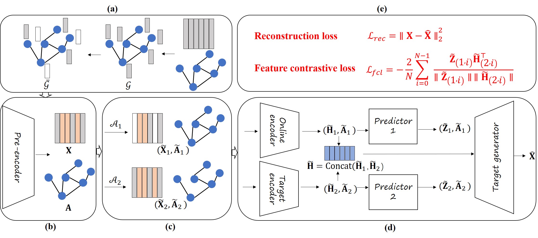
Figure 1. The AmGCL framework. Firstly, the attribute missing graph $\bar{\mathcal{G}}$ is input into the precoder for feature encoding, resulting in a feature vector $(\mathbf{X},\mathbf{A})$. Then, using the augmented distribution method, the augmented features $(\widetilde{\mathbf{X}}_{1},\widetilde{\mathbf{A}}_{1})$ and $(\widetilde{\mathbf{X}}_{2},\widetilde{\mathbf{A}}_{2})$ are obtained and input into the GACLS module. In the GACLS module, the augmented features are encoded using the online encoder and target encoder, resulting in latent features $\widetilde{\mathbf{H}}_{1}$ and $\widetilde{\mathbf{H}}_{2}$, respectively. These features are then merged into $\widetilde{\mathbf{H}}$, which is decoded by the target generator to obtain the reconstructed node attribute features $\hat{\mathbf{X}}$.

In the feature precoding, the model employs the Dirichlet energy minimisation method to predict missing node attributes for subsequent graph representation learning. In the attribute graph augmentation, the model uses graph augmentation methods to enhance the robustness and generalisation of the model. The GACLS module uses self-supervised graph contrastive learning methods to learn the latent variable representations of nodes, and target generator to reconstruct the features. Finally, in the loss optimization, the model employs reconstruction loss and feature contrastive loss function to improve contrast sensitivity and model robustness during training.

3.1. Preliminary

Observing from Figure 1 (a), we define the attribute graph $\mathcal{G}$, the set of nodes is denoted as $\mathcal{V(G)}=\{v_{1},...,v_{n}\}$, and the set of edges as $\mathcal{E(G)}=\{e_{1},...,e_{n}\}$. Edge $e_{ij}$ connects nodes $v_{i}$ and $v_{j}$, and $\mathcal{N}(i)=\{v_{j}:(v_{i},v_{j})\in\mathcal{E}\}$ represents the neighbor set of node $v_{i}$. Each node has a $d$-dimensional feature vector $\mathbf{X}\in\mathbb{R}^{N\times d}$ representing its attribute features. The attribute missing graph $\bar{\mathcal{G}}$ has two sets of nodes: $\mathcal{V}^{o}=\{v_{1}^{o},v_{2}^{o},...,v_{N_{o}}^{o}\}$ and $\mathcal{V}^{m}=\{v_{1}^{m},v_{2}^{m},...,v_{N_{m}}^{m}\}$, representing the sets of nodes with observed and missing attributes, respectively. The node set in the graph is denoted as $\mathcal{V}=\mathcal{V}^{o}\cup\mathcal{V}^{m}$, with $\mathcal{V}^{o}$ and $\mathcal{V}^{m}$ being disjoint sets, and $N=N_{o}+N_{m}$. The attribute feature vectors for the observed and missing node sets are denoted by $\mathbf{X}^{o}$ and $\mathbf{X}^{m}$, respectively. We aim to perform feature imputation and node classification on graphs with missing attributes in this paper. Our method involves using the available observed attribute values to interpolate the missing ones, while ensuring that the resulting embedding is suitable for the subsequent node classification task.

3.2. Feature Precoding

In attribute graphs, the node’s attribute features are usually represented as high-dimensional vectors. Directly inputting missing attribute features into the network may cause network redundancy and introduce noise. Many feature imputation methods have been proposed, including imputation, matrix completion-based methods (Xu et al., 2015), and graph-based methods (Chen et al., 2022). In this paper, we introduce a feature precoding method based on Dirichlet energy minimization (Jeffreys et al., 1999). The advantage is that it can effectively estimate missing features by utilizing the structural similarity and connectivity between nodes.

As shown in Figure 1 (b), before performing feature precoding, the features of each node need to be initialized. In this paper, the node’s feature vector is initialized with its true feature, and for missing nodes, it is initialized with a zero vector. Next, for each node $v_{i}$, the contribution of its neighboring nodes $v_{j}\in\mathcal{N}(v_{i}^{o})$ to its features is calculated, and these contributions are accumulated to obtain a new feature vector $\mathbf{X}_{i}$, which represents the feature of node $i$ after one round of feature precoding. This process can be calculated by:

(1) $$\mathbf{X}_{i}^{(l+1)}=\mathbf{X}_{i}^{(l)}+\sum_{j\in\mathcal{N}\left(v_{i}^{o}\right)}w_{ij}\left(\mathbf{X}_{j}^{(l)}-\mathbf{X}_{i}^{(l)}\right)$$

where $w_{ij}$ is a normalization factor that balances the degree difference between different nodes, and $l$ represents the number of iterations. Generally, multiple rounds of feature precoding can result in more accurate node features. Therefore, we iterate the above steps multiple times until convergence or until the predetermined number of iterations is reached. In this paper, the number of iterations is set to 40.

3.3. Attribute Graph Augmentation

When an attribute graph contains missing values, node features may not fully reflect the true state of the nodes. Therefore, attribute graph augmentation can improve learning performance on attribute graphs by adding meaningful edges or removing irrelevant edges to improve the graph structure.

As shown in Figure 1 (c), by applying two random graph augmentation functions $\mathcal{A}_{1}$ and $\mathcal{A}_{2}$ to produce two alternative views of $\mathcal{G}$:

(2) $$\left({\widetilde{\mathbf{X}}}_{1},{\widetilde{\mathbf{A}}}_{1}\right)=\mathcal{A}_{1}(\mathbf{X}_{1},\mathbf{A}_{1}),$$

$$\left({\widetilde{\mathbf{X}}}_{2},{\widetilde{\mathbf{A}}}_{2}\right)=\mathcal{A}_{2}(\mathbf{X}_{2},\mathbf{A}_{2}).$$

Attribute graph augmentation can be considered in two ways: feature masking (You et al., 2020a) and edge dropout (Zhu et al., 2020). Feature masking can reduce the interference of noise on the model by masking some node features. Edge dropout can reduce noise interference and redundant information by deleting edges, thereby improving the quality and stability of node features. Specifically, in the attribute graph missing problem, feature masking and edge dropout can remove noise edges that may interfere with learning, reducing the negative impact of attribute graph missing on node feature learning. These augmentations are graph-level and do not operate on each node independently, leveraging graph topology information.

3.4. GACLS

To learn the informative latent representation of the data and improve the model’s generalization performance, we propose a GACLS as the training network (Figure 1 (d)), inspired by BYOL (Grill et al., 2020). GACLS uses two graph encoders: an online encoder $E_{\theta}$ and a target encoder $E_{\phi}$, with different parameters $\theta$ and $\phi$. The online encoder generates an online representation, $\widetilde{\mathbf{H}}1:=E_{\theta}(\widetilde{\mathbf{X}}_{1},\widetilde{\mathbf{A}}_{1})$, from the first augmented graph, while the target encoder generates a target representation, $\widetilde{\mathbf{H}}2:=E_{\phi}(\widetilde{\mathbf{X}}_{2},\widetilde{\mathbf{A}}_{2})$, from the second augmented graph. The output of the online network is passed through a predictor to obtain a prediction vector, and the output of the target network is used as the target vector for the predictor, updated via a slow-moving average to make the online and target network outputs approach each other in latent space. The online representation is then inputted into the predictor $p_{\theta}$, which outputs a prediction for the online representation, $\widetilde{\mathbf{Z}}_{1}:=p_{\theta}(\widetilde{\mathbf{H}}_{1})$. It is worth noting that the predictor works at the node level and does not use graph information (i.e., it only operates on $\widetilde{\mathbf{H}}_{1}$ and not $\widetilde{\mathbf{A}}_{1}$). Similarly, the prediction of the target representation is $\widetilde{\mathbf{Z}}_{2}:=p_{\theta}(\widetilde{\mathbf{H}}_{2})$.

By combining GACLS with the attribute graph feature missing problem, we train the online and target networks to learn latent vector representations for feature prefilling of missing node attributes. These vectors are then merged and inputted into a target generator to reconstruct the missing features.

3.5. Loss Optimization

AmGCL requires an effective loss function to guide model training. To improve model learning, AmGCL employs a comprehensive loss function that comprises two components, namely reconstruction loss and feature contrastive loss ( Figure 1 (e)). The reconstruction loss is guided by the principle of Dirichlet energy minimisation and is used to guide the model on known attribute features, aiming to enable the model to better predict the attribute features of missing nodes. On the other hand, the feature contrastive loss aims to maximise the lower bound on mutual information evidence and is used to guide the model in learning the similarity of feature representations to improve the model’s performance in node classification tasks.

3.5.1. Feature Contrastive Loss

To bring the prediction closer to the true target while avoiding model collapse, we update the online parameter $\theta$ using the gradient of the cosine similarity relative to the online encoder, while the parameter $\phi$ of the target encoder is updated using an exponential moving average of the online parameter $\theta$. The feature contrastive loss function can be expressed as:

(3) $$\mathcal{L}_{\text{fcl}}=-\frac{2}{N}\sum_{i=0}^{N-1}\frac{p\left(\widetilde{\mathbf{H}}_{(1,i)}\right)\widetilde{\mathbf{H}}_{(2,i)}^{\top}}{\left\|p\left(\widetilde{\mathbf{H}}_{(1,i)}\right)\right\|\left\|\widetilde{\mathbf{H}}_{(2,i)}\right\|},$$

where $\widetilde{\mathbf{H}}_{1}^{i}$ represents the representation of input data $\mathbf{X}_{i}$ obtained through the online network, while $\widetilde{\mathbf{H}}_{2}^{i}$ represents the representation of input data $\mathbf{X}_{i}$ obtained through the target network. $p(\cdot)$ is the predictor, and $N$ is the batch size. These two representations are concatenated into an embedding representation $\widetilde{\mathbf{H}}$, which is defined as $\widetilde{\mathbf{H}}:=[\widetilde{\mathbf{H}}_{1},\widetilde{\mathbf{H}}_{2}]$, where $[\cdot,\cdot]$ denotes the vector concatenation operation. By minimizing the loss functions of the predictor network and the target network, AmGCL can learn the latent representation of the data and apply it to downstream tasks. AmGCL’s performance on the Steam dataset is poor due to the low network connectivity, which makes it difficult for the model to capture attributes through the network structure.

3.5.2. Reconstruction Loss

Feature reconstruction is a widely used training technique in self-supervised learning, where the original feature vector is first mapped to another vector and then reconstructed back through inverse mapping. The reconstruction loss, which employs Dirichlet energy minimisation, measures the difference between the reconstructed feature and the original feature. Its objective is to minimize the reconstruction error of the network, so that the learned features can retain the information of the original features and be utilized for downstream tasks.

To be specific, we feed the latent feature vector $\mathbf{H}$ into a target generator $D_{\mu}$ composed of a multi-layer perceptron (MLP). The target generator aims to map the feature vector to another vector $\hat{\mathbf{X}}:=D_{\mu}(\mathbf{H})$ and then reconstruct it back through inverse mapping. Therefore, we employ the mean squared error (MSE) as the loss function between the online network and the reconstructor, which can be represented as:

(4) $$\mathcal{L}_{\text{rec}}=\frac{1}{N}\sum_{i=0}^{N-1}\left\|\mathbf{X}_{i}-\widehat{\mathbf{X}}_{i}\right\|_{2}^{2}.$$

The comprehensive loss function can be represented as:

(5) $$\mathcal{L}=\mathcal{L}_{\text{rec}}+\lambda\mathcal{L}_{\text{fcl}},$$

where $\lambda$ is the hyperparameter that controls the weight of the two loss components. Detailed theoretical proofs can be found in Appendix A.

4. Experimentation and analysis

In this section, we address the following research questions:

Q1: How does AmGCL perform on feature imputation tasks? (Section 4.4)

Q2: What are the results of AmGCL on node classification tasks? (Section 4.5)

Q3: How does AmGCL generalize and perform under different rates of missing input data? (Section 4.6.1)

Q4: What is the role of each module in AmGCL, as evaluated through ablation studies? (Section 4.6.2)

Q5: What is the contribution of the two loss functions to the performance of AmGCL, as evaluated through ablation studies? (Section 4.6.3)

Q6: What is the computational complexity of AmGCL and how does it compare to other state-of-the-art methods? (Section 4.7)

4.1. Datasets

We have selected six publicly available graph datasets as the experimental objects in this study, each of which contains important information such as nodes, edges, features and subgraphs. The graph structure and node features of these datasets have been widely used in various tasks such as node classification and representation learning. We conducted a brief data statistics and analysis, and the specific situation is shown in Table 1.

Table 1. Data statistics.

Dataset	Nodes	Edges	Feature	Classes	Subgraphs
Cora	2,708	10,556	1,433	7	78
CiteSeer	3,327	9,104	3,703	6	438
PubMed	19,717	88,648	500	3	1
CS	18,333	163,788	6,805	15	1
Computers	13,752	491,722	767	10	314
Photo	7,650	238,162	745	8	136
Seam	9,944	266,981	352	-	6,741

The Cora dataset (Yang et al., 2016) is a widely used benchmark for evaluating the performance of graph-based machine learning algorithms.

The CiteSeer dataset (Yang et al., 2016) is a digital library and search engine focused on computer and information science literature. The CiteSeer dataset is often used to evaluate graph-based machine learning algorithms.

The PubMed dataset (Yang et al., 2016) is a benchmark for evaluating machine learning algorithms for scientific literature analysis.

The CS dataset (Shchur et al., 2018) is based on the Microsoft Academic Graph co-authorship network, using data provided by the KDD Cup 2016 challenge. In this dataset, each node represents an author, and if two authors co-authored a paper, there is an edge connecting these two nodes. The node features represent the paper keywords for each author, while the labels indicate the author’s most active research area.

The Computers and Photo datasets (Shchur et al., 2018) are fragments of the Amazon co-purchasing graph, where nodes represent products and edges indicate frequent co-purchasing of two products. The node features are bag-of-words encoded product reviews, and the labels are given by the product categories.

The Steam dataset (Chen et al., 2022) contains 9944 games and 352 tags. The co-purchasing frequency between every two games was calculated based on user purchasing behavior, and a sparse item co-purchasing graph was obtained by binarizing the co-purchasing frequency using a threshold of 10.

Table 2. Feature imputation results on attribute missing graph with 60% missing data.

Metric	Method	Type	Cora			CiteSeer			Computers			Photo			Steam
			@10	@20	@50	@10	@20	@50	@10	@20	@50	@10	@20	@50	@3	@5	@10
Recall	NeighAggre	Aggregation	0.0906	0.1413	0.1961	0.0511	0.0908	0.1501	0.0321	0.0593	0.1306	0.0329	0.0616	0.1361	0.0603	0.0881	0.1446
	VAE	Generation	0.0887	0.1228	0.2116	0.0382	0.0668	0.1296	0.0255	0.0502	0.1196	0.0276	0.0538	0.1279	0.0564	0.0820	0.1251
	GNN*	Representation	0.1350	0.1812	0.2972	0.0620	0.1097	0.2058	0.0273	0.0533	0.1278	0.0295	0.0573	0.1324	0.2395	0.3431	0.4575
	GraphRNA	Generation	0.1395	0.2043	0.3142	0.0777	0.1272	0.2271	0.0386	0.0690	0.1465	0.0390	0.0703	0.1508	0.2490	0.3208	0.4372
	ARWMF	Generation	0.1291	0.1813	0.2960	0.0552	0.1015	0.1952	0.0280	0.0544	0.1289	0.0294	0.0568	0.1327	0.2104	0.3201	0.4512
	FP	Aggregation	0.1571	0.2224	0.3338	0.0851	0.1368	0.2283	0.0425	0.0741	0.1544	0.0434	0.0773	0.1627	0.2095	0.2733	0.3664
	SAT	Generation	0.1653	0.2345	0.3612	0.0811	0.1349	0.2431	0.0421	0.0746	0.1577	0.0427	0.0765	0.1635	0.2536	0.3620	0.4965
	SVGA	Generation	0.1718	0.2486	0.3814	0.0943	0.1539	0.2782	0.0437	0.0769	0.1602	0.0446	0.0798	0.1670	0.2565	0.3602	0.4996
	AmGCL	Contrast	0.1811	0.2536	0.3852	0.1031	0.1636	0.2819	0.0441	0.0769	0.1603	0.0449	0.0798	0.1669	0.2673	0.3621	0.5067
NDCG	NeighAggre	Aggregation	0.1217	0.1548	0.1850	0.0823	0.1155	0.1560	0.0788	0.1156	0.1923	0.0813	0.1196	0.1998	0.0955	0.1204	0.1620
	VAE	Generation	0.1224	0.1452	0.1924	0.0601	0.0839	0.1251	0.0632	0.0970	0.1721	0.0675	0.1031	0.1830	0.0902	0.1133	0.1437
	GNN*	Representation	0.1736	0.2076	0.2702	0.1026	0.1423	0.2049	0.0671	0.1027	0.1824	0.0705	0.1082	0.1893	0.3366	0.4138	0.4912
	GraphRNA	Generation	0.1934	0.2362	0.2938	0.1291	0.1703	0.2358	0.0931	0.1333	0.2155	0.0959	0.1377	0.2232	0.3437	0.4023	0.4755
	ARWMF	Generation	0.1824	0.2182	0.2776	0.0859	0.1245	0.1858	0.0694	0.1053	0.1851	0.0727	0.1098	0.1915	0.3066	0.3877	0.4704
	FP	Aggregation	0.2220	0.2668	0.3249	0.1409	0.1861	0.2445	0.1051	0.1473	0.2332	0.1061	0.1508	0.2411	0.2674	0.2377	0.2855
	SAT	Generation	0.2250	0.2723	0.3394	0.1385	0.1834	0.2545	0.1030	0.1463	0.2346	0.1047	0.1498	0.2421	0.3585	0.4400	0.5272
	SVGA	Generation	0.2381	0.2894	0.3601	0.1579	0.2076	0.2892	0.1068	0.1509	0.2397	0.1084	0.1549	0.2472	0.3567	0.4391	0.5299
	AmGCL	Contrast	0.2507	0.2979	0.3644	0.1734	0.2239	0.3019	0.1082	0.1516	0.2404	0.1090	0.1549	0.2469	0.3595	0.4222	0.5011

4.2. Baselines

We compared AmGCL with several existing baseline models in our study. NeighAgg (Şimşek and Jensen, 2008) is a classic method that aggregates the features of adjacent nodes by mean pooling. For the case of missing neighbor attributes, we exclude them from the node aggregation. We only use one-hop neighbors as node neighbors. VAE (Kingma and Welling, 2013) is a generative model that learns the latent representation of instances. For test nodes with no attributes, we use neighbor aggregation methods (e.g., NeighAggre) to obtain the aggregated latent code of the test node in the latent space. Then, we use the decoder in VAE to reconstruct the missing node attributes. GCN (Kipf and Welling, 2016), GraphSAGE (Hamilton et al., 2017), and GAT (Veličković et al., 2017) are popular graph neural networks that have been widely applied in various domains. For simplicity, we refer to the best-performing models in these three models as GNN*. GraphRNA (Huang et al., 2019) and ARWMF (Chen et al., 2019) are recent representation learning methods that can be used for feature generation. FP (Rossi et al., 2022) represents the feature precoding method, which uses Dirichlet energy minimization to fill in missing features. SAT (Chen et al., 2022) uses a shared latent space to train independent autoencoders that provide a shared latent space for features and graph structure, respectively. SVGA (Yoo et al., 2022) is a state-of-the-art feature estimation model that establishes the feature space of features and graph structure by introducing Gaussian Markov random fields.

We divided AmGCL into two versions. AmGCL* is a variant that only uses $\mathcal{L}_{\text{fcl}}$ as the loss function and uses $\hat{\mathbf{X}}$ as the input for downstream classification. AmGCL’s loss function is $\mathcal{L}_{\text{fcl}}+\mathcal{L}_{\text{rec}}$, and it uses $\widetilde{\mathbf{H}}$ as the input for downstream classification.

4.3. Experimental Setup

AmGCL uses masking to represent missing feature attributes. Unless otherwise stated, we treat 40% of the observable data as the training set and consider 60% of the attribute missing nodes as target nodes (missing attribute nodes) and split them into validation and test sets in a 1:5 ratio, as in previous work (Yoo et al., 2022). We employ different experimental procedures for feature imputation and node classification.

For feature imputation, the latent layer dimension of each GNN and linear layer is set to 128. We run each experiment 10 times and report the average results. Each experiment runs for a maximum of 1000 epochs, and we use the Adam optimizer with a learning rate of 0.001 to train the model for the best results.

For node classification, we use the target nodes and their induced subgraphs (i.e., edges that only involve the target nodes) and divide the data set into training and testing sets in an 8:2 ratio, performing 5-fold cross-validation on the target nodes. We run a maximum of 1000 epochs and evaluate the quality of the generated features based on the accuracy of node classification. We use GCN as the classifier, with 2 layers, a dropout rate of 0.2, and a latent layer dimension of 256. We also use the Adam optimizer with a learning rate of 0.001 to train the model.

4.4. Feature Imputation Results

High-quality reconstructed attributes should have a high probability similar to that of real attributes in a given dimension. We conducted experiments on missing features and used Recall@k and NDCG@k as evaluation metrics for the discrete feature dataset. Specifically, we set k = {10, 20, 30} for Cora, CiteSeer, Computers, and Photo datasets, and k = {3, 5, 10} for the Steam dataset. The results of feature estimation are presented in Table 2. By comparing with the baseline, we observed that our method outperformed the others in most cases.

Based on the evaluation results, NeighAggre and VAE performed the worst as they failed to achieve robust learning results at the attribute level, indicating that they were not effective in representing node features. GCN achieved good results, indicating that it can better capture the correlations between node features and effectively learn node representations. Random walk based attribute aggregation methods such as GraphRNA and ARWMF can capture the correlations in the attribute dimensions, but the statistical noise introduced by random walks may lead to moderate results. SAT and SVGA, as advanced deep generative models, focus on solving the problem of missing attribute graphs and have achieved some competitiveness in the results. AmGCL performed the best in most cases because it uses a more effective network structure and loss function. We conducted an analysis to understand why AmGCL did not perform as well on Steam dataset, and found that poor connectivity within the graph hindered the propagation of features along the graph structure.

4.5. Node Classification Results

In the node classification task on the attribute missing graph, we select the target node features that perform the best on the Recall@10 metric for node classification. From the table, it can be seen that (1) methods such as VAE, GCN, GraphSAGE, GAT, and Hers perform poorly because they are not specifically designed for missing attribute graphs. (2) Methods such as GraphRNA, AEWMF, SAT, and SVGA, which are specifically designed for attribute missing graphs, achieve certain results, but our method performs the best.

From Table 3, it can be seen that AmGCL* outperforms AmGCL and achieves the state of the art. The loss function in AmGCL* only includes $\mathcal{L}_{\text{fcl}}$ without the feature reconstruction part, achieving the SOTA in node classification. This is because the node features themselves already contain enough information to distinguish different node categories. Therefore, the results of the node classification task may not be significantly affected by feature reconstruction, and even feature reconstruction may have a negative impact on classification. However, AmGCL* may not be able to utilize the diversity of learning tasks with node features. Therefore, it is still necessary to combine $\mathcal{L}_{\text{fcl}}$ with $\mathcal{L}_{\text{rec}}$ to obtain good results in both classification performance and feature reconstruction. The role of the two loss functions will be further reported in the ablation experiments.

Table 3. Node classification results.

Method	Cora	CiteSeer	PubMed	CS	Computers	Photo
NeighAggre	0.6494	0.5413	0.6564	0.8031	0.8715	0.9010
VAE	0.3011	0.2663	0.4007	0.2335	0.4023	0.3781
GCN	0.4387	0.4079	0.4203	0.2180	0.3974	0.3656
GraphSage	0.5779	0.4278	0.4200	0.2335	0.4019	0.3784
GAT	0.4525	0.2688	0.4196	0.2334	0.4034	0.3789
GraphRNA	0.8198	0.6394	0.8172	0.8851	0.8650	0.9207
ARWMF	0.8025	0.2764	0.8089	0.8347	0.7400	0.6146
SAT	0.8579	0.6767	0.7439	0.8402	0.8766	0.9260
SVGA	0.8533	0.6879	0.6287	0.9037	0.8845	0.9272
AmGCL	0.8848	0.7703	0.8180	0.9040	0.8870	0.9281
AmGCL*	0.9179	0.7932	0.8525	0.9232	0.8871	0.9320

4.6. Ablation Experiments

We comprehensively evaluate the performance and generalization ability of each module of the model from three aspects: data ablation, GACLS model ablation, and loss function ablation.

4.6.1. Data ablation

To validate the effectiveness of in AmGCL across different data scenarios, we trained the model under missing rates ranging from 0.2 to 0.8 and evaluated the performance in terms of node classification. The results are shown in Table 4. “AmGCL w/ RF” denotes using both observable and newly generated features as output, while “AmGCL w/o FP” denotes not using the initial feature precoding module. From Table 4, it can be observed that (1) AmGCL achieved the best performance in most cases, and its ablations outperformed SVGA. (2) Using both the original observable features and newly generated missing features as the output can improve the accuracy of node classification. (3) Removing data feature propagation from the feature pre-coding module may have a negative impact on the results.

Table 4. Data ablation results.

Method	Missing	Cora	CiteSeer	PubMed	CS	Computers	Photo
SVGA	0.2	0.9243	0.7018	0.6167	0.9133	0.8754	0.9318
	0.4	0.9177	0.7277	0.5790	0.9101	0.8813	0.9314
	0.6	0.9006	0.6574	0.6287	0.9054	0.8845	0.9272
	0.8	0.8763	0.6423	0.6060	0.9009	0.8810	0.9281
AmGCL	0.2	0.9498	0.8822	0.8739	0.9543	0.9095	0.9497
	0.4	0.9443	0.8603	0.8671	0.9443	0.9049	0.9393
	0.6	0.9347	0.8223	0.8614	0.9435	0.9015	0.9349
	0.8	0.9180	0.7472	0.8566	0.9218	0.8951	0.9275
AmGCL w/o FP	0.2	0.9471	0.8747	0.8650	0.9775	0.8934	0.9409
	0.4	0.9408	0.8523	0.8559	0.9719	0.8881	0.9347
	0.6	0.9305	0.8343	0.8322	0.9517	0.8879	0.9348
	0.8	0.9121	0.7240	0.8034	0.9258	0.8814	0.9233
AmGCL w/ RF	0.2	0.9653	0.9162	0.8726	0.9781	0.9346	0.9597
	0.4	0.9612	0.9053	0.8609	0.9726	0.9276	0.9552
	0.6	0.9542	0.8548	0.8518	0.9603	0.9200	0.9448
	0.8	0.9232	0.7707	0.8435	0.9421	0.9048	0.9349

Table 5 presents the performance of different methods on the node classification task when the node feature missing rate is 0.95. Raw denotes the original data, SVGA and FP are the two comparative methods, and AmGCL is the proposed method in this paper. From the table, it can be seen that the accuracy of AmGCL is higher than SVGA and the original data on all datasets. The FP method performs well on some datasets, indicating that AmGCL has good generalization performance, i.e., it can maintain high accuracy even in extremely missing data scenarios. Meanwhile, the performance of SVGA on some datasets is worse than the original data, indicating that SVGA has poor generalization ability.

Table 5. Data ablation experiments at a missing rate of 0.95.

Method	Cora	CiteSeer	PubMed	CS	Computers	Photo
Raw	0.6440	0.4481	0.6746	0.7354	0.8468	0.8841
SVGA	0.4760	0.2185	0.6226	0.8864	0.8426	0.9089
FP	0.8667	0.6360	0.8198	0.9160	0.8777	0.9119
AmGCL	0.9054	0.6651	0.8354	0.9217	0.8790	0.9146

4.6.2. GACLS Module Ablation

Results of GACLS model ablation experiments are presented in Table 6. “w/o generator” indicates removing the target generator structure and directly using $\widetilde{\mathbf{H}}$ as the output; “w/o concat” means using only $\widetilde{\mathbf{H}}_{1}$ as the output; “w/o concat + generator” means removing the generator structure and using both $\widetilde{\mathbf{H}}_{1}$ as the output; “w/o FM” means not using feature masking for graph augmentation; “w/o ER” means not using edge removal for graph augmentation. The results clearly demonstrate that AmGCL outperforms the others in most cases.

Table 6. Results of GACLS model ablation experiments.

Type	Cora	CiteSeer	PubMed	CS	Computers	Photo
w/o generator	0.9070	0.7818	0.8488	0.9176	0.8991	0.9339
w/o concat	0.9243	0.8170	0.8490	0.9417	0.8987	0.9348
w/o concat +generator	0.8977	0.7731	0.8309	0.9145	0.8845	0.9285
w/o FM	0.9265	0.8209	0.8526	0.9413	0.9031	0.9388
w/o ER	0.9158	0.8197	0.8483	0.9411	0.8978	0.9348
AmGCL	0.9347	0.8223	0.8614	0.9435	0.9088	0.9349

4.6.3. Loss Function Ablation

Tables 7 and 8 present the results of the loss ablation experiments on feature reconstruction. As observed from the tables, the feature reconstruction performance slightly decreases when the $L_{\text{fcl}}$ loss is removed, indicating the positive impact of $L_{\text{fcl}}$ loss on improving feature reconstruction. However, a significant improvement in the node classification metrics was observed when the $L_{\text{rec}}$ loss was further removed, suggesting that the $L_{\text{rec}}$ loss interferes with the node classification task. The feature interpolation is important and must not be overlooked. Therefore, the combination of $L_{\text{fcl}}$ and $L_{\text{rec}}$ can strike a balance between the node classification and feature reconstruction tasks, leading to better performance.

Table 7. Reconstruction loss ablation results.

Metric	Method	CiteSeer			Computers			Photo
		@10	@20	@50	@10	@20	@50	@10	@20	@50
Recall	w/o $\mathcal{L}_{\text{fcl}}$	0.0974	0.1585	0.2744	0.0422	0.0742	0.1560	0.0436	0.0776	0.1651
	AmGCL	0.1030	0.1627	0.2809	0.0434	0.0762	0.1587	0.0442	0.0784	0.1648
NDCG	w/o $\mathcal{L}_{\text{fcl}}$	0.1674	0.2166	0.2928	0.1030	0.1457	0.2331	0.1063	0.1514	0.2441
	AmGCL	0.1729	0.2229	0.3010	0.1058	0.1494	0.2375	0.1072	0.1525	0.2438

Table 8. Feature contrastive loss ablation results.

Method	Cora	CiteSeer	PubMed	CS	Computers	Photo
AmGCL	0.9095	0.7971	0.8563	0.9017	0.8877	0.9304
w/o $\mathcal{L}_{\text{rec}}$	0.9542	0.8548	0.8518	0.9603	0.9200	0.9448

4.7. Method Performance Validation

To further evaluate the performance of the model, we compared the training time and computational resources required by the model, as shown in Table 9 below. The complexity analysis of the AmGCL is shown in Appendix B.

From the Table 9, we can see that the number of training parameters required by the AmGCL method is much smaller than the other two methods on different datasets. For example, on the PubMed dataset, the AmGCL method has only 243,203 parameters, which is much less than the 4,195,309 parameters of the SAT method and the 5,301,519 parameters of the SVGA method. In addition, we can also see that the number of parameters required by the AmGCL method on the Cora, CiteSeer, and Photo datasets is also much less than the other two generative methods. This means that the AmGCL method can be trained and deployed faster while requiring less computational resources.

The Table 9 provides information on the training time required by the three methods on various datasets. It is evident that the AmGCL method outperforms the other two methods in terms of training time. Specifically, on the CiteSeer, Computers, and Photo datasets, the AmGCL method takes significantly less time to train than the other methods.

More detailed experimental analysis can be found in Appendices C, D and E.

Table 9. Model parameters and training time statistics.

Type	Method	Cora	CiteSeer	PubMed	CS	Computers	Photo
Params	SAT	1,167,642	2,201,712	4,195,309	3,109,376	3,109,376	1,880,154
	SVGA	1,136,060	1,877,245	5,301,519	6,560,215	3,826,728	2,240,166
	AmGCL	602,499	1,473,923	243,203	2,667,395	347,523	338,563
Times	SAT	3.5661	4.3805	6.3210	8.5790	8.5791	5.7879
	SVGA	3.3365	3.4780	4.3585	10.7354	10.6048	7.2488
	AmGCL	2.9250	3.2108	4.1859	7.6305	7.8639	4.5042

5. Conclusion

This paper proposes an AmGCL method to address the node attribute missing problem in attribute missing graph data. AmGCL deals with the problem of missing node attributes by combining Dirichlet energy minimisation and contrastive learning methods, which has not been applied by other existing methods. AmGCL uses feature precoding and a GACLS to learn potential representations of missing nodes, which can improve the performance of attribute graph analysis tasks by filling in missing node attributes while preserving the overall graph structure. Experimental results demonstrate that on multiple real-world datasets, AmGCL outperforms state-of-the-art methods in terms of feature imputation and node classification. Future work will explore how well feature interpolation can be combined with downstream tasks to fully exploit attribute missing graph learning.

Appendix A Research Methods

A.1. Mutual Information Proof

GACLS is inspired by BYOL, which can be treated as a kind of non-negtive-sampling contrastive learning. And contrastive learning is essentially maximizing the mutual information of positive sample pair.

For a specific subgraph $c$, take 1 positive sample graph or augment and $N-1$ negative samples from N different distributions respectively, then the probability that $x_{i}$ is a positive sample is:

(6) $$p\left(d=i\mid X,c\right) =\frac{p\left(x_{i}\mid c\right)\prod_{l\neq i}p\left(x_{l}\right)}{\sum_{j=1}^{N}p\left(x_{j}\mid c\right)\prod_{l\neq j}p\left(x_{l}\right)}$$

$$=\frac{\frac{p\left(x_{i}\mid c\right)}{p\left(x_{i}\right)}}{\sum_{j=1}^{N}\frac{p\left(x_{j}\mid c\right)}{p\left(x_{j}\right)}}$$

It can be seen from the following formula that the goal of contrastive learning optimization is to maximize the mutual information lower bound.

(7) $$\mathcal{L}_{\mathrm{N}}^{\mathrm{opt}} =-\underset{X}{\mathbb{E}}\log\left[\frac{\frac{p\left(x_{i}\mid c\right)}{p\left(x_{i}\right)}}{\frac{p\left(x_{i}\mid c\right)}{p\left(x_{i}\right)}+\sum_{x_{j}\in X_{\mathrm{ncg}}}\frac{p\left(x_{j}\mid c\right)}{p\left(x_{j}\right)}}\right]$$

$$=\underset{X}{\mathbb{E}}\log\left[1+\frac{p\left(x_{i}\right)}{p\left(x_{i}\mid c\right)}\sum_{x_{j}\in X_{\text{neg }}}\frac{p\left(x_{j}\mid c\right)}{p\left(x_{j}\right)}\right]$$

$$\approx\underset{X}{\mathbb{E}}\log\left[1+\frac{p\left(x_{i}\right)}{p\left(x_{i}\mid c\right)}(N-1)\underset{x_{j}}{\mathbb{E}}\frac{p\left(x_{j}\mid c\right)}{p\left(x_{j}\right)}\right]$$

$$=\underset{X}{\mathbb{E}}\log\left[1+\frac{p\left(x_{i}\right)}{p\left(x_{i}\mid c\right)}(N-1)\right]$$

$$\geq\underset{X}{\mathbb{E}}\log\left[\frac{p\left(x_{i}\right)}{p\left(x_{i}\mid c\right)}N\right]$$

$$=-I\left(x_{i},c\right)+\log(N)$$

A.2. Dirichlet Energy Proofs

The feature precoding method is based on Dirichlet energy minimization. The recursive relation can be deduced as follows.

(8) $$\min_{X}\mathcal{L}= \sum_{(i,j)\in\mathcal{E}}w_{ij}(x_{i}-x_{j})^{2}=\text{tr}(X^{T}LX)$$

$$\text{s.t. }X_{k}=Z_{k}$$

$$\implies \mathcal{L^{\prime}}=LX=(I-\widetilde{A})X=0,\quad X_{k}=Z_{k}$$

$$\implies X=\widetilde{A}X,\quad X_{k}=Z_{k}$$

Appendix B Method Complexity Analysis

Analyzing the time and space complexity of AmGCL as shown in Table 10, where the number of attributes is $F$, the number of edges $|\mathcal{E}|$, the number of nodes $|\mathcal{V}|$, the number of categories $c$, and the dimension of the latent variable $d$, it can be seen from the table that the time complexity of AmGCL is $O(F|\mathcal{E}|+(Fd+d^{2})|\mathcal{V}|)$ and the space complexity is $O(|\mathcal{E}|+(d+F)|\mathcal{V}|+d^{2}+Fd)$.

Table 10. Complexity analysis on AmGCL.

Module	Time	Space
Precoder * 1	$O(F|\mathcal{E}|)$	$O(|\mathcal{E}|+F|\mathcal{V}|)$
Augment * 2	$O(|\mathcal{E}|+|\mathcal{V}|)$	$O(|\mathcal{E}|+F)$
Encoder * 2	$O((F+d)(|\mathcal{E}|+d|\mathcal{V}|))$	$O(|\mathcal{E}|+d^{2}+d|\mathcal{V}|)$
Predictor * 2	$O(d^{2}|\mathcal{V}|)$	$O(d^{2})$
Generator * 1	$O(Fd|\mathcal{V}|)$	$O(Fd+F|\mathcal{V}|)$

Appendix C Experiments on Rational Motivation of AmGCL

Table 11. Experimental results on the proof of model motivation.

Metric	Method	Cora			CiteSeer			Computers			Photo
		@10	@20	@50	@10	@20	@50	@10	@20	@50	@10	@20	@50
Recall	BYOL	0.1456	0.2118	0.3430	0.0794	0.1324	0.2472	0.0407	0.0727	0.1537	0.0421	0.0751	0.1601
	BYOL+One hot	0.1402	0.2073	0.3321	0.0705	0.1190	0.2205	0.0410	0.0730	0.1543	0.0410	0.0739	0.1578
	BYOL+Dirichlet	0.1341	0.1909	0.2981	0.0597	0.0914	0.1563	0.0314	0.0545	0.1164	0.0313	0.0565	0.1202
	Precoder	0.1571	0.2224	0.3338	0.0851	0.1368	0.2283	0.0425	0.0741	0.1544	0.0434	0.0773	0.1627
	SAT	0.1653	0.2345	0.3612	0.0811	0.1349	0.2431	0.0421	0.0746	0.1577	0.0427	0.0765	0.1635
	SVGA	0.1718	0.2486	0.3814	0.0943	0.1539	0.2782	0.0437	0.0769	0.1602	0.0446	0.0798	0.1670
	AmGCL	0.1811	0.2507	0.3752	0.1031	0.1636	0.2819	0.0441	0.0769	0.1603	0.0449	0.0798	0.1669
nDCG	BYOL	0.2040	0.2481	0.3172	0.1277	0.1719	0.2472	0.0996	0.1420	0.2282	0.1023	0.1461	0.2360
	BYOL+One hot	0.1942	0.2390	0.3048	0.1190	0.1595	0.2260	0.1005	0.1431	0.2299	0.0999	0.1436	0.2325
	BYOL+Dirichlet	0.1954	0.2335	0.2905	0.1038	0.1305	0.1732	0.0784	0.1098	0.1764	0.0781	0.1119	0.1801
	Precoder	0.2220	0.2668	0.3249	0.1409	0.1861	0.2445	0.1051	0.1473	0.2332	0.1061	0.1508	0.2411
	SAT	0.2250	0.2723	0.3394	0.1385	0.1834	0.2545	0.1030	0.1463	0.2346	0.1047	0.1498	0.2421
	SVGA	0.2381	0.2894	0.3601	0.1579	0.2076	0.2892	0.1068	0.1509	0.2397	0.1084	0.1549	0.2472
	AmGCL	0.2507	0.2977	0.3641	0.1734	0.2239	0.3019	0.1082	0.1516	0.2404	0.1090	0.1549	0.2469

This section analyzes the design process of AmGCL through experiments to better illustrate our contribution. The pseudo code of AmGCL is shown in Algorithm 1.

Input: Attribute-missing graph $\bar{\mathcal{G}}$, adjacency matrix $\mathbf{A}$, and observable node features $\mathbf{X}^{o}$, Iteration number $I$.

Output: Reconstructed features $\hat{\mathbf{X}}$, embedded features $\widetilde{\mathbf{H}}$.

1 Initialize the parameters of GACLS;

2 Perform feature precoder on $\mathbf{X}^{o}$ to obtain $\mathbf{X}$;

3 for  $i=1$ to $I$  do

4       Enhance $\mathbf{A}$ and $\mathbf{X}$ using graph enhancement algorithms $\mathcal{A}_{1}$ and $\mathcal{A}_{2}$ to obtain (${\widetilde{\mathbf{X}}}_{1}{,\ \widetilde{\mathbf{A}}}_{1}$) and (${\widetilde{\mathbf{X}}}_{2}{,\ \widetilde{\mathbf{A}}}_{2}$);

5       Use the Online encoder and Target encoder of GACLS to calculate (${\widetilde{\mathbf{H}}}_{1}{,\ \widetilde{\mathbf{A}}}_{1}$) and (${\widetilde{\mathbf{H}}}_{2}{,\ \widetilde{\mathbf{A}}}_{2}$);

6       Input (${\widetilde{\mathbf{H}}}_{1}{,\ \widetilde{\mathbf{A}}}_{1}$) and (${\widetilde{\mathbf{H}}}_{2}{,\ \widetilde{\mathbf{A}}}_{2}$) into the predictor to obtain (${\widetilde{\mathbf{Z}}}_{1}{,\ \widetilde{\mathbf{A}}}_{1}$) and (${\widetilde{\mathbf{Z}}}_{2}{,\ \widetilde{\mathbf{A}}}_{2}$);

7       Combine ${\widetilde{\mathbf{H}}}_{1},\ {\widetilde{\mathbf{H}}}_{2}$ to obtain $\widetilde{\mathbf{H}}$;

8       Input $\widetilde{\mathbf{H}}$ into the generator to obtain $\hat{\mathbf{X}}$;

9       Use Equations 3 and 4 for contrastive learning and reconstruction learning;

10       Back propagation and update parameters;

11      

12 end for

13Return $\hat{\mathbf{X}}$ and $\widetilde{\mathbf{H}}$;

Algorithm 1 Training process of AmGCL.

Overall design motivation: Firstly, we notice that the state-of-the-art methods, SAT and SVGA, both impose restrictions on latent variables during reconstruction, with SAT using GAN and SVGA using GMRF. Although this is effective in some cases, it can lead to overfitting in other cases due to overly strict limitations. In contrast, AmGCL uses self-supervised contrastive learning for feature interpolation, without explicitly modeling or restricting the latent variables, but rather through mutual information constraints. This makes AmGCL more flexible and robust, able to adapt to various data distributions and missing patterns.

Model design: Pre-encoder: For attribute missing graphs, we focus on the fact that the original distribution of features is disrupted, so the setting of the initial distribution is crucial. To build the initial distribution of features, AmGCL adopts a pre-encoder based on minimizing the Dirichlet energy. This pre-encoder uses graph structural information to propagate features, obtaining the initial feature representation for each node. Compared to traditional methods such as random padding or taking the mean, the pre-encoder can make more full use of graph structural information, rather than just attribute features. It can also adopt different orders of neighbors by controlling the number of propagation layers. Since the pre-encoder has no training parameters, it can be easily embedded into the entire architecture of AmGCL.

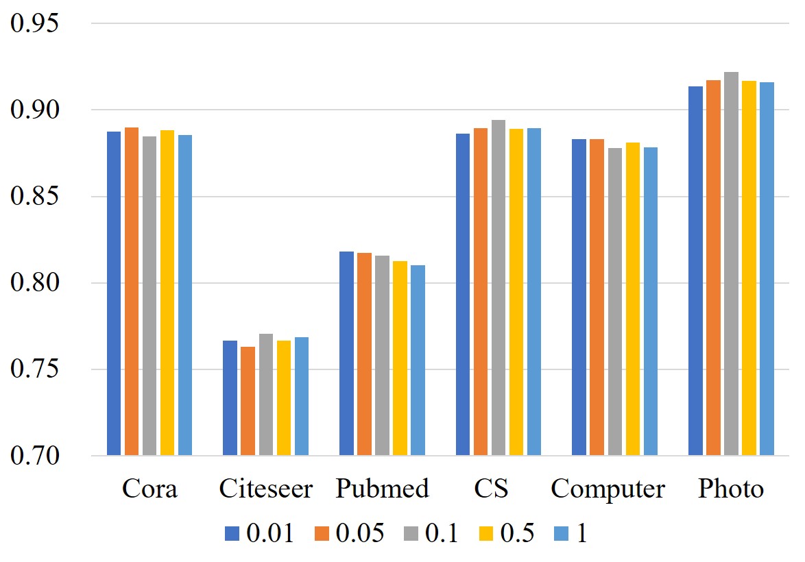
Figure 2. Equilibrium parameter $\lambda$ results.

GACLS: This architecture is the core of AmGCL, drawing on the idea of BYOL and using self-supervised contrastive learning for feature interpolation. Specifically, GACLS first encodes node features using an online and target encoder architecture, obtaining the latent feature representation. Then, by feeding the latent feature representation into the generator and removing the irrelevant components of mutual information based on energy minimization, the reconstructed feature representation is obtained.

We conducted experiments to fully demonstrate the effectiveness of the modules. From Table 11, “BYOL” represents using the BYOL framework, and initializing features as learnable parameters following a Gaussian distribution, training with both contrastive and reconstruction losses. “BYOL+One hot” feature represents initializing features as a one-hot encoding matrix on the basis of “BYOL”. “BYOL+Dirichlet” represents incorporating Dirichlet energy minimization into the training loss on the basis of “BYOL”, rather than representing it in the form of a pre-encoder. “Precoder” represents using only the pre-encoder for feature propagation as the final output. From the results, it can be seen that the performance of “BYOL” is significantly lower than that of AmGCL, because it requires more training parameters and has a larger search space. Both “BYOL+One hot” and “BYOL+Dirichlet” are inferior to using “BYOL” alone, which reversely proves the role of the pre-encoder. Meanwhile, “Precoder” has certain competitiveness, which also indicates that Dirichlet energy minimization is effective. The fact that AmGCL based on contrastive learning outperforms SAT and SVGA based on generative learning also demonstrates the effectiveness of self-supervised contrastive learning for attribute missing graph learning.

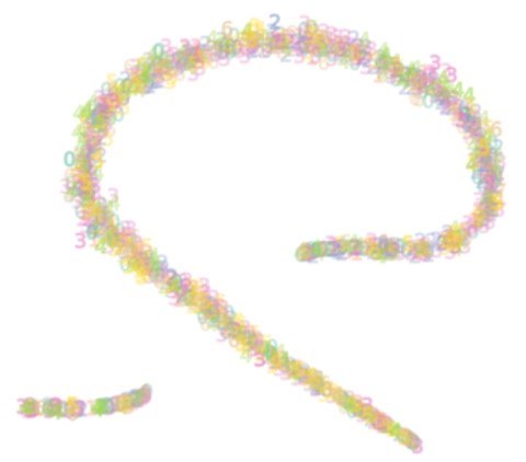
(a) SAT

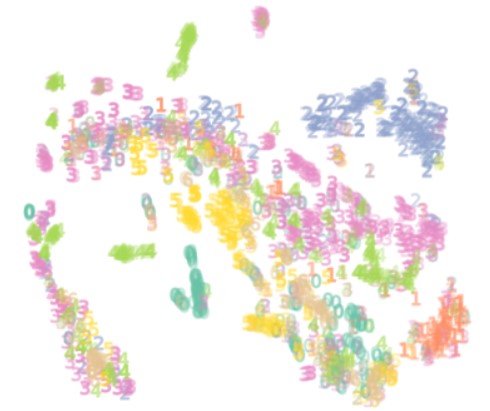
(b) SVGA

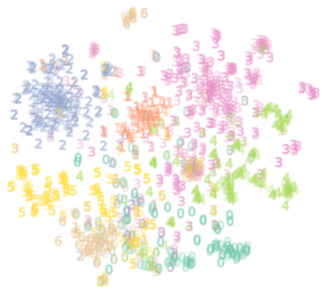
(c) AmGCL

Figure 3. Visual comparison of interpolation features.

Appendix D Hyperparameter Settings

We have analysed the equilibrium parameters of the loss function and the results are shown in Figure 2.

Appendix E Interpolation Feature Visualization

Since SAT and SVGA were the most advanced methods in previous experiments on attribute-missing graph learning, they were chosen as the most representative methods for comparison with AmGCL. We visualized the distribution of learned node embeddings for all three methods on all datasets using t-SNE (Van der Maaten and Hinton, 2008). As shown in Figure 3, AmGCL exhibits a clearer structure and better reveals the intrinsic data structure compared to the baseline.

References

- (1)
- Cai et al. (2010) Jian-Feng Cai, Emmanuel J Candès, and Zuowei Shen. 2010. A singular value thresholding algorithm for matrix completion. SIAM Journal on optimization 20, 4 (2010), 1956–1982.
- Candes and Recht (2012) Emmanuel Candes and Benjamin Recht. 2012. Exact matrix completion via convex optimization. Commun. ACM 55, 6 (2012), 111–119.
- Chen et al. (2019) Lei Chen, Joan Bruna, and Michael Bronstein. 2019. Attributed random walk as matrix factorization. In Proceedings of the International Conference on Neural Information Processing Systems, Graph Representation Learning Workshop.
- Chen et al. (2022) Xu Chen, Siheng Chen, Jiangchao Yao, Huangjie Zheng, Ya Zhang, and Ivor W Tsang. 2022. Learning on Attribute-Missing Graphs. IEEE Transactions on Pattern Analysis and Machine Intelligence 44, 2 (2022), 740–757.
- Cheng et al. (2022) Dawei Cheng, Fangzhou Yang, Sheng Xiang, and Jin Liu. 2022. Financial time series forecasting with multi-modality graph neural network. Pattern Recognition 121 (2022), 108218.
- Garcia Satorras et al. (2019) Victor Garcia Satorras, Zeynep Akata, and Max Welling. 2019. Combining Generative and Discriminative Models for Hybrid Inference. In Proceedings of the International Conference on Neural Information Processing Systems. Curran Associates, Inc., 1–11.
- Grill et al. (2020) Jean-Bastien Grill, Florian Strub, Florent Altché, Corentin Tallec, Pierre H Richemond, Elena Buchatskaya, Carl Doersch, Bernardo Avila Pires, Zhaohan Daniel Guo, Mohammad Gheshlaghi Azar, et al. 2020. Bootstrap your own latent a new approach to self-supervised learning. In Proceedings of the International Conference on Neural Information Processing Systems. 21271–21284.
- Hamilton et al. (2017) William L Hamilton, Rex Ying, and Jure Leskovec. 2017. Inductive representation learning on large graphs. In Proceedings of the International Conference on Neural Information Processing Systems. 1025–1035.
- Hastie et al. (2015) Trevor Hastie, Rahul Mazumder, Jason D Lee, and Reza Zadeh. 2015. Matrix completion and low-rank SVD via fast alternating least squares. The Journal of Machine Learning Research 16, 1 (2015), 3367–3402.
- He et al. (2020) Xiangnan He, Kuan Deng, Xiang Wang, Yan Li, Yongdong Zhang, and Meng Wang. 2020. Lightgcn: Simplifying and powering graph convolution network for recommendation. In Proceedings of the International ACM SIGIR conference on research and development in Information Retrieval. 639–648.
- Huang et al. (2019) Xiao Huang, Qingquan Song, Yuening Li, and Xia Hu. 2019. Graph recurrent networks with attributed random walks. In Proceedings of the ACM SIGKDD International Conference on Knowledge Discovery & Data Mining. 732–740.
- Jeffreys et al. (1999) Harold Jeffreys, Bertha Jeffreys, and Bertha Swirles. 1999. Methods of mathematical physics. Cambridge university press.
- Jin et al. (2022) Di Jin, Rui Wang, Tao Wang, Dongxiao He, Weiping Ding, Yuxiao Huang, Longbiao Wang, and Witold Pedrycz. 2022. Amer: A New Attribute-Missing Network Embedding Approach. IEEE Transactions on Cybernetics (2022).
- Kingma and Welling (2013) Diederik P Kingma and Max Welling. 2013. Auto-encoding variational bayes. arXiv preprint arXiv:1312.6114 (2013).
- Kipf and Welling (2016) Thomas N Kipf and Max Welling. 2016. Semi-supervised classification with graph convolutional networks. arXiv preprint arXiv:1609.02907 (2016).
- Krasnova et al. (2010) Hanna Krasnova, Sarah Spiekermann, Ksenia Koroleva, and Thomas Hildebrand. 2010. Online social networks: Why we disclose. Journal of information technology 25, 2 (2010), 109–125.
- Liu et al. (2020) Fan Liu, Zhiyong Cheng, Lei Zhu, Chenghao Liu, and Liqiang Nie. 2020. An attribute-aware attentive GCN model for attribute missing in recommendation. IEEE Transactions on Knowledge and Data Engineering 34, 9 (2020), 4077–4088.
- Myers et al. (2014) Seth A Myers, Aneesh Sharma, Pankaj Gupta, and Jimmy Lin. 2014. Information network or social network? The structure of the Twitter follow graph. In Proceedings of the International Conference on World Wide Web. 493–498.
- Rossi et al. (2022) Emanuele Rossi, Henry Kenlay, Maria I Gorinova, Benjamin Paul Chamberlain, Xiaowen Dong, and Michael M Bronstein. 2022. On the unreasonable effectiveness of feature propagation in learning on graphs with missing node features. In Learning on Graphs Conference. PMLR, 11–1.
- Shannon (2001) Claude Elwood Shannon. 2001. A mathematical theory of communication. ACM SIGMOBILE Mobile Computing and Communications Review 5, 1 (2001), 3–55.
- Shchur et al. (2018) Oleksandr Shchur, Maximilian Mumme, Aleksandar Bojchevski, and Stephan Günnemann. 2018. Pitfalls of graph neural network evaluation. arXiv preprint arXiv:1811.05868 (2018).
- Shi et al. (2021) Hongkuan Shi, Zhiwei Wang, Jinxin Lv, Yilang Wang, Peng Zhang, Fei Zhu, and Qiang Li. 2021. Semi-supervised Learning via Improved Teacher-Student Network for Robust 3D Reconstruction of Stereo Endoscopic Image. In Proceedings of the ACM International Conference on Multimedia. 4661–4669.
- Silva-Ramírez et al. (2015) Esther-Lydia Silva-Ramírez, Rafael Pino-Mejías, and Manuel López-Coello. 2015. Single imputation with multilayer perceptron and multiple imputation combining multilayer perceptron and k-nearest neighbours for monotone patterns. Applied Soft Computing 29 (2015), 65–74.
- Şimşek and Jensen (2008) Özgür Şimşek and David Jensen. 2008. Navigating networks by using homophily and degree. Proceedings of the National Academy of Sciences 105, 35 (2008), 12758–12762.
- Spinelli et al. (2020) Indro Spinelli, Simone Scardapane, and Aurelio Uncini. 2020. Missing data imputation with adversarially-trained graph convolutional networks. Neural Networks 129 (2020), 249–260.
- Taguchi et al. (2021) Hibiki Taguchi, Xin Liu, and Tsuyoshi Murata. 2021. Graph convolutional networks for graphs containing missing features. Future Generation Computer Systems 117 (2021), 155–168.
- Van der Maaten and Hinton (2008) Laurens Van der Maaten and Geoffrey Hinton. 2008. Visualizing data using t-SNE. Journal of Machine Learning Research 9, 11 (2008).
- Veličković et al. (2017) Petar Veličković, Guillem Cucurull, Arantxa Casanova, Adriana Romero, Pietro Lio, and Yoshua Bengio. 2017. Graph attention networks. arXiv preprint arXiv:1710.10903 (2017).
- Vincent et al. (2010) Pascal Vincent, Hugo Larochelle, Isabelle Lajoie, Yoshua Bengio, Pierre-Antoine Manzagol, and Léon Bottou. 2010. Stacked denoising autoencoders: Learning useful representations in a deep network with a local denoising criterion. Journal of Machine Learning Research 11, 12 (2010).
- Xia et al. (2017) Jing Xia, Shengyu Zhang, Guolong Cai, Li Li, Qing Pan, Jing Yan, and Gangmin Ning. 2017. Adjusted weight voting algorithm for random forests in handling missing values. Pattern Recognition 69 (2017), 52–60.
- Xu et al. (2021) Cai Xu, Hongmin Liu, Ziyu Guan, Xunlian Wu, Jiale Tan, and Beilei Ling. 2021. Adversarial incomplete multiview subspace clustering networks. IEEE Transactions on Cybernetics 52, 10 (2021), 10490–10503.
- Xu et al. (2015) Chang Xu, Dacheng Tao, and Chao Xu. 2015. Multi-view learning with incomplete views. IEEE Transactions on Image Processing 24, 12 (2015), 5812–5825.
- Yang et al. (2016) Zhilin Yang, William Cohen, and Ruslan Salakhudinov. 2016. Revisiting semi-supervised learning with graph embeddings. In Proceedings of the International Conference on Machine Learning. PMLR, 40–48.
- Yoo et al. (2022) Jaemin Yoo, Hyunsik Jeon, Jinhong Jung, and U Kang. 2022. Accurate Node Feature Estimation with Structured Variational Graph Autoencoder. In Proceedings of the ACM SIGKDD Conference on Knowledge Discovery and Data Mining. 2336–2346.
- Yoon et al. (2018) Jinsung Yoon, James Jordon, and Mihaela Schaar. 2018. Gain: Missing data imputation using generative adversarial nets. In Proceedings of the International Conference on Machine Learning. PMLR, 5689–5698.
- You et al. (2020b) Jiaxuan You, Xiaobai Ma, Daisy Yi Ding, Mykel Kochenderfer, and Jure Leskovec. 2020b. Handling missing data with graph representation learning. In Proceedings of the International Conference on Neural Information Processing Systems. 19075–19087.
- You et al. (2020a) Yuning You, Tianlong Chen, Yongduo Sui, Ting Chen, Zhangyang Wang, and Yang Shen. 2020a. Graph contrastive learning with augmentations. In Proceedings of the International Conference on Neural Information Processing Systems. 5812–5823.
- Zhang and Chen (2018) Muhan Zhang and Yixin Chen. 2018. Link prediction based on graph neural networks. In Proceedings of the International Conference on Neural Information Processing Systems. 5171–5181.
- Zhu et al. (2020) Yanqiao Zhu, Yichen Xu, Feng Yu, Qiang Liu, Shu Wu, and Liang Wang. 2020. Deep graph contrastive representation learning. arXiv preprint arXiv:2006.04131 (2020).