, ,
On the analysis of Rayleigh-Bénard convection using Latent Dirichlet Allocation
Abstract
We apply a probabilistic clustering method, Latent Dirichlet Allocation (LDA), to characterize the large-scale dynamics of Rayleigh-Bénard convection. The method, introduced in Frihat et al. 2021, is applied to a collection of snapshots in the vertical mid-planes of a cubic cell for Rayleigh numbers in the range . For the convective heat flux, temperature and kinetic energy, the decomposition identifies latent factors, called motifs, which consist of connex regions of fluid. Each snapshot is modelled with a sparse combination of motifs, the coefficients of which are called the weights. The spatial extent of the motifs varies across the cell and with the Rayleigh number. We show that the method is able to provide a compact representation of the heat flux and displays good generative properties. At all Rayleigh numbers the dominant heat flux motifs consist of elongated structures located mostly within the vertical boundary layer, at a quarter of the cavity height. Their weights depend on the orientation of the large-scale circulation (LSC). A simple model relating the conditionally averaged weight of the motifs to the relative strength of the corner rolls and of the large-scale circulation, is found to predict well the average LSC reorientation rate. Application of LDA to the temperature fluctuations shows that temperature motifs are well correlated with heat flux motifs in space as well as in time, and to some lesser extent with kinetic energy motifs. The abrupt decrease of the reorientation rate observed at is associated with a strong concentration of plumes impinging onto the corners of the cell, which decrease the temperature difference within the corner structures. It is also associated with a reinforcement of the longitudinal wind through formation and entrainment of new plumes.
I Introduction
Rayleigh-Bénard convection, in which a fluid is heated from below and cooled from above, represents an idealized configuration to study thermal convection phenomena. These characterize a variety of applications ranging from industrial processes such as heat exchangers to geophysical flows in the atmosphere or the ocean. A central question is to determine how the heat transfer depends on nondimensional parameters such as the Prandtl number where is the kinematic viscosity and the thermal diffusitivity, and the Rayleigh number
| (1) |
where is the gravity, is the thermal expansion coefficient, the temperature difference and the cell dimension. The Grossmann and Lohse [1] theory constitutes a unified approach to address this question. It is based on a local description of the physics: the contributions from the bulk averaged thermal and kinetic dissipation rate are split into two subsets, one corresponding to the boundary layers, and one corresponding to the bulk. This theory was further refined in Grossmann and Lohse [2], where the thermal dissipation rate was split into a contribution from the plumes and a contribution from the turbulent background. Through the action of buoyancy, the thermal boundary layers generate plumes which create a large-scale circulation, as evidenced by Xi et al. [3], also called ”wind” [4]. The distribution of temperature fluctuations depends on plume clustering effects [5], but it is also affected by interaction with turbulent fluctuations in the bulk, resulting in fragmentation [6].
Shang et al. [7] showed that plume-dominated regions were located near the sidewalls and the conducting surfaces and that thermal plumes carry most of the convective heat flux, which contributes to the production of both kinetic and thermal fluctuations. The morphology of plumes and its effect on the heat transfer have been given careful attention. The plumes have a sheet-like structure near the boundary layer and progressively become mushroom-like as they move into the bulk region [8]. Shishkina and Wagner [9] found that very high values of the local heat flux were observed in regions where the sheet-like plumes merged, constituting ”stems” for the mushroom-like plumes developing in the bulk. The relative contributions of the plumes and turbulent background vary with the Rayleigh number: Emran and Schumacher [10] have shown that the fraction of plume-dominated regions decreases with the Rayleigh number, while that of background-dominated regions increases.
The identification of local coherent structures such as plumes is therefore an essential step for the understanding of thermal convection flows. Several definitions have been used: some of the first criteria were based on the skewness of the temperature derivative [11] or the temperature difference [12]. Ching et al. [13] have proposed to use simultaneous measurements of the temperature and the velocity to define the velocity of the plumes using conditional averaging. Following Huang et al. [14], van der Poel et al. [15] identified plumes from both a temperature anomaly and an excess of convective heat flux. [16] relied on cliff-ramp-like structures in the temperature signals to determine the spatial characteristics of plumes. Emran and Schumacher [10] and Vishnu et al. [17] separated the plume from the background regions based on a threshold on the convective heat flux. Shevkar et al. [18] have recently proposed a dynamic criterion based on the 2-D velocity divergence to separate plumes from boundary layers.
As pointed out by Chilla and Schumacher [19], this multiplicity of criteria illustrates the difficulty of identifying coherent structures in a consistent and objective manner, which is a long-running question in various types of turbulent flows. To this end, Proper Orthogonal Decomposition (POD) [20] has proven a useful tool to analyze large-scale fluctuations in Rayleigh-Bénard convection. It has been used in particular to study reorientations of the large-scale circulation [21, 22, 23, 24, 25]. Through spectral decomposition of the autocorrelation tensor, POD provides a basis of spatial modes, also called empirical modes, since they originate from the data. The modes are energetically optimal to reconstruct the fluctuations. The POD modes typically have a global support, which is well suited to capture the large-scale organization of the flow. However, this can make physical interpretation difficult as there is no straightforward connection between a mode and a local coherent structure as a local structure is represented with a superposition of many POD modes, a situation also observed in Fourier analysis. Soucasse et al. [26] have used POD to study the dynamics of the large-scale circulation for Rayleigh numbers in the range . They found that although the reorientation rate varied with the Rayleigh number, the dominant structures remained similar across that range, albeit with some variations in their energy. A new dissipation-based POD decomposition, proposed by Olesen et al. [27] and applied to Rayleigh-Bénard convection [28], highlighted the importance of boundary layers for the dynamics, which points to the need for local descriptions.
As an alternative, Frihat et al. [29] have recently adapted a probabilistic method that can extract localized latent factors in turbulent flow measurements. This method, Latent Dirichlet Allocation or LDA [30, 31], was originally developed in the context of natural language processing, where it aims to extract topics from a collection of documents. In this framework, documents are represented by a non-ordered set of words taken from a fixed vocabulary. A word count matrix can be built for the collection, where each column corresponds to a document, each line corresponds to a vocabulary word and the matrix entry represents the number of times the word appears in the document. LDA provides a probabilistic decomposition of the word count matrix, based on latent factors called topics. Topics are defined by two distributions: the distribution of topics within each document (each document is associated with a mixture of topics, the coefficients of the mixture sum up to one) and the distribution of vocabulary words with each topic (each topic is represented by a combination of words, the coefficients of which also sum up to one).
The method has been adapted for turbulent flows as follows: we consider a collection of snapshots of a scalar field taken over a 2D domain discretized into cells. The equivalent of a document is therefore a snapshot, and the cells (or snapshot pixels) constitute the vocabulary. The digitized values of the scalar field over the cells in a snapshot are gathered into a vector which is formally analogous to a column of the word count matrix. The ”topics” produced by the decomposition, called motifs, correspond to fixed (in the Eulerian sense), spatially coherent regions of the flow. The method was found to be well suited for the representation of intermittent data (Frihat et al. [29], Fery et al. [32]). It was succesfully applied to the analysis of the turbulent Reynolds stress in wall turbulence [29]. Moreoever, the method provides a local description that is insensitive to the existence of global symmetries. It proved a useful tool to identify synoptic objects in weather data [32].
In this paper, we apply this method to the analysis of fluctuations in a cubic Rayleigh-Bénard cell in the range of Rayleigh number . The goal is to track the local signature of the large-scale dynamics of the flow, and to determine whether changes can be identified as the Rayleigh number increases. To this end, the technique is applied to 2D sections of a cubic Rayleigh-Bénard cell in the range of Rayleigh number . The numerical configuration and the data set are described in Section 2. We first present the method for the convective heat flux, using a comparison with POD to highlight the similarities and differences of the approach. Proper Orthogonal Decomposition (POD) and Latent Dirichlet Allocation (LDA) are respectively presented in Section 3 and 4. We examine in Section 5 how LDA compares with POD and the extent to which it is able to capture the general features of the heat flux. The characteristics of heat flux motifs and their connection with the reorientations of the large-scale circulation are discussed in Section 6. The analysis is then extended to temperature fluctuations and to the kinetic energy in Section-7 in order to provide further insight into the physics. A conclusion is given in section 8.
II Numerical setting
II.1 Set-up
Numerical setup and associated datasets are the same as used in Soucasse et al. [25, 26]. The configuration studied is a cubic Rayleigh-Bénard cell filled with air, with isothermal horizontal walls and adiabatic side walls. The air is assumed to be transparent and thermal radiation effects are disregarded. Direct numerical simulations have been performed at various values of the Rayleigh number. The Prandtl number is set to 0.707. All physical quantities are made dimensionless using the cell size , the reference time and the reduced temperature , being the mean temperature between hot and cold walls. Spatial coordinates are denoted , , ( being the vertical direction) and the origin is placed at a bottom corner of the cube.
Navier–Stokes equations under Boussinesq approximation are solved using a Chebyshev collocation method [33, 34]. Computations are made parallel using domain decomposition along the vertical direction. Time integration is performed through a second-order semi-implicit scheme. The velocity divergence-free condition is enforced using a projection method. Numerical parameters are given in Table 1 for the four considered Rayleigh numbers . We have checked that the number of collocation points is sufficient to accurately discretize the boundary layers according to the criterion proposed by [35]. A number of 1000 snapshots have been extracted from the simulations for each Rayleigh number at a sampling period of 10 (at ) or 5 (at ), in dimensionless time units. It is worth noting that the time separation between the snapshots is sufficient to describe the evolution of the large-scale circulation but is not suited for a fine description of the plume emission or of the reorientation process. For each Rayleigh number, a dataset satisfying the statistical symmetries of the flow was then constructed from these 1000 snapshots, as will be described in the next section.
| (81,81,81) | 1000 | 10 | 0.056 | |
| (81,81,81) | 1000 | 10 | 0.042 | |
| (81,81,81) | 1000 | 10 | 0.0297 | |
| (161,161,161) | 1000 | 5 | 0.0167 |
II.2 Construction of the data set
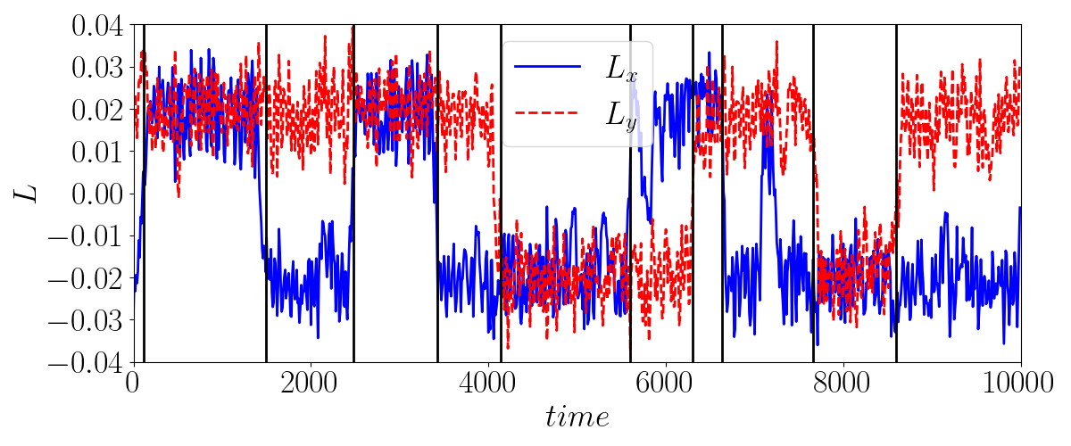
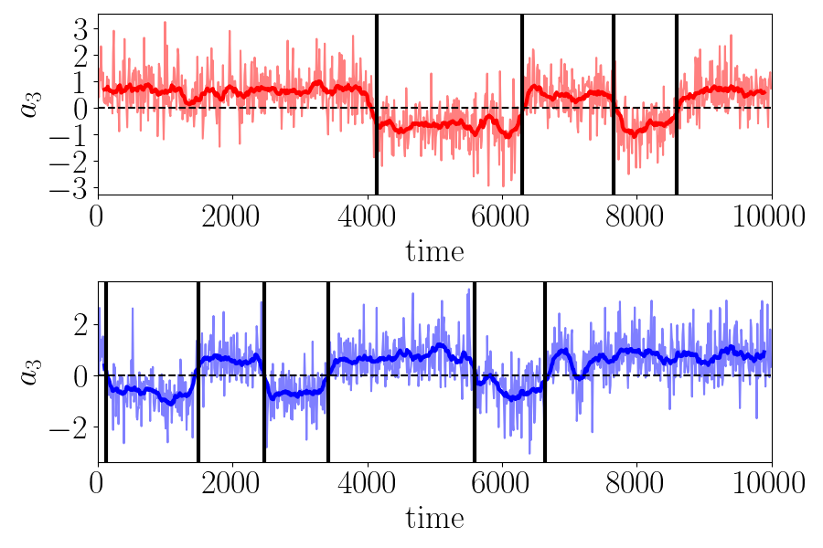
At each Rayleigh number, the data set consisted of a collection of snapshots , . Results will be presented first for the convective heat flux , then for the temperature fluctuations ( being the time-averaged temperature) and for the kinetic energy , , and being the velocity components. We note that due to the velocity reference scale, the non-dimensional heat flux varies like . As in Soucasse et al. [25], the data set was first enriched by making use of the statistical symmetries of the flow [36]. In the cubic Rayleigh-Bénard cell, four quasi-stable states are available for the flow for this Rayleigh number range: the large-scale circulation settles in one of the two diagonal planes of the cube with clockwise or counterclockwise motion. The evolution of the large-scale circulation can be tracked through that of the and components of the angular momentum of the cell with respect to the cell center . As Figure 1 shows at , the angular momentum along each horizontal direction oscillates near a quasi-steady position for long periods of times - several hundreds of convective time scales, before experiencing a rapid switch ( convective time scales) to the opposite value, which corresponds to a reorientation. On each plane we can define an indicator function , which takes the value where is the angular momentum component normal to the plane.
Reorientations from one state to another occur during the time sequence but each state is not necessarily equally visited. In order to counteract this bias, we have built enlarged snapshot sets, obtained by the action of the symmetry group of the problem on the original snapshot sets. The symmetries are based on four independent symmetries , , and with respect to the planes , , and . This generates a group of 16 symmetries for the cube, which should lead to a 16-fold in the number of snapshots. However, since we will exclusively consider the vertical mid-planes and , which are invariant planes for respectively and , the increase is reduced. The data set aggregates 1000 snapshots on each of the planes and , each of which undergoes a vertical flip, a horizontal flip and a combination of the two, yielding a total of snapshots.
The LDA technique requires transforming the data into a non-negative, integer field. The signal defined on a grid of cells was digitized using a rescaling factor . If the field was not of constant sign (temperature, heat flux), positive and negative values were split onto two distinct grids, leading to a field defined on cells. For the heat flux, this gives
| (2) | |||||
| (3) |
where , and and represents the cell location on the mid-planes or . We note that throughout the paper, the total field will directly be represented on the physical grid of size from the renormalized difference .
III POD analysis
III.1 Method
Proper Orthogonal Decomposition [37] makes it possible to write a collection of spatial fields defined on grid points, as a superposition of spatial modes , the amplitude of which varies in time:
| (4) |
with and . The amplitudes are solution of the eigenvalue problem
| (5) |
where is the temporal autocorrelation matrix
| (6) |
The eigenvalues , such that , represent the respective contribution of the modes to the total variance. If we consider the most energetic modes, the reconstruction based on modes minimizes the -norm error between the set of snapshots and the projection of the set of snapshots onto a basis of size .
III.2 Application to the convective heat flux
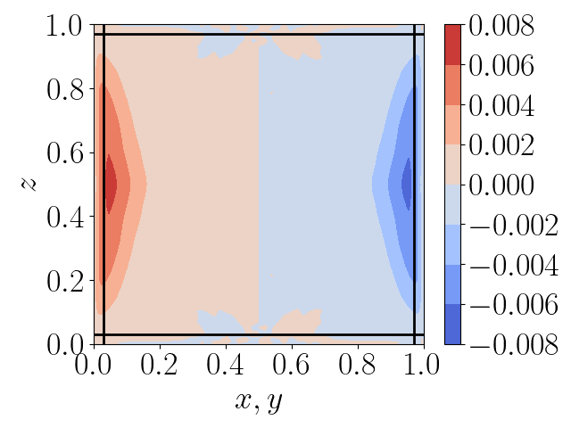
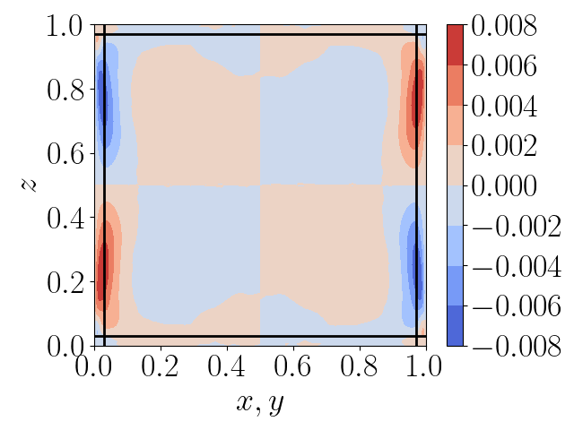
POD is applied to the digitized heat flux signal defined in equations (2) and (3). The first three POD modes and POD coefficients are shown in Figure 2 for , where black vertical and horizontal lines indicate the thickness of the boundary layers. We checked that the first mode corresponds to the mean flow. The mode is most important in a region close to the wall, with a maximum within the vertical boundary layer at a height of about . The second mode corresponds to a dissymetry between the vertical sides and is most important at mid-height in the region outside the boundary layers. The third mode is both antisymmetric in the vertical and in the horizontal direction. It is maximum at the edge of the vertical boundary layers, at a vertical distance of about from the horizontal surfaces. The pattern it is associated with corresponds to a more intense flux along a diagonal (bottom of one side and top of the opposite side) and a less intense flux along the opposite diagonal. As evidenced by application of a moving average performed over 200 convective time units (about 4 recirculation times , as was determined in Soucasse et al. [25]), the evolution of the amplitude at large time scales matches that of the horizontal angular momentum components and (compare with Figure 1), unlike the two dominant modes. This mode therefore appears to be the signature of the large-scale circulation, where the flux is more intense in the lower corner of the cell as hot plumes rise on one side and in the upper corner of the opposite side of the cell as cold plumes go down.
IV Latent Dirichlet Allocation
IV.1 Principles
We briefly review the principles of Latent Dirichlet Allocation and refer the reader to Frihat et al. [29] for more details. LDA is an inference approach to identify latent factors in a collection of observed data, which relies on Dirichlet distributions as priors. We first recall the definition of a Dirichlet distribution, which is a multivariate probability distribution over the space of multinomial distributions. It is parameterized by a vector of positive-valued parameters as follows
| (7) |
where is a normalizing factor, which can be expressed in terms of the Gamma function :
| (8) |
The components of control the sparsity of the distribution: values of larger than unity correspond to evenly dense distributions, while values lower than unity correspond to sparse distributions. Here will represent either the motif-cell distribution or the snapshot-motif distribution.
As mentioned above, the data to which LDA is applied consists of a collection of non-negative, integer fields that are defined in equations (2) and (3). For each snapshot , the integer value measured at cell is interpreted as an integer count of the cell . The key is to interpret this integer count as the number of times cell appears in the composition of snapshot . A snapshot is therefore defined as a list of tuples of the form .
The main assumptions of LDA are the following:
-
1.
Each snapshot consists of a mixture of latent factors called motifs. is a user-defined parameter (analogous to a number of clusters).
-
2.
Each motif is associated with a multinomial distribution over the grid cells so that the probability to observe the grid cell located at given the motif is . The distribution is modelled with a Dirichlet prior parameterized with an -dimensional vector . Low values of mean that the motif is distributed over a small number of cells.
-
3.
Each snapshot is associated with a distribution over motifs such that the probability that motif is present in snapshot will be denoted . This distribution is modelled with a -dimensional Dirichlet distribution of parameter . The magnitude of characterizes the sparsity of the distribution. Low values of mean that relatively few motifs are observed in each snapshot.
IV.2 Implementation
The snapshot–motif distribution and the motif-cell distribution are determined from the observed snapshots and constitute and -dimensional categorical distributions. Finding the distributions and that are most compatible with the observations constitutes an inference problem. The problem can be solved either with a Markov chain Monte-Carlo (known as MCMC) algorithm such as Gibbs sampling [30], or by a variational approach [31], which aims to minimize the Kullback–Leibler divergence between the true posterior and its variational approximation. In both cases, the computational complexity of the problem of the order of .
The solution a priori depends on the number of motifs as well as on the values of the Dirichlet parameters and . Special attention was therefore given to establish the robustness of the results reported here. Non-informative default values were used for the Dirichlet parameters i.e. the prior distributions were taken with symmetric parameters equal to and . Practical implementation was performed in Python using gensim [38]. No significant change was observed in the results when the value of the quantization was high enough (however it had to be kept reasonably low in order to limit the computational time). Although multiple tests were carried out for varying values of , all results reported in this paper were obtained with for the heat flux. Values of and were respectively used for the temperature fluctuations and for the kinetic energy. Analyses were also performed for varying numbers of motifs , ranging from 50 to 400.
IV.3 LDA as a generative process
The standard generative process performed by LDA with motifs is the following.
-
For each motif , a -dimensional cell–motif distribution is drawn from the Dirichlet distribution of parameter .
-
To generate snapshot :
-
a -dimensional snapshot–motif distribution is drawn according to a Dirichlet distribution parameterized by
-
a total integer count is drawn. This number corresponds to the total number of cell integer counts associated with snapshot i.e. . is typically sampled from a Poisson distribution that matches the statistics of the original database.
-
for each :
-
*
a motif is selected from (since represents the probability that motif is present in the snapshot)
-
*
once this motif is chosen, a cell is selected from (since represents the probability that cell is present in motif )
-
*
-
The snapshot then represents the set of cells that have been drawn and can be reorganized as a list of cells with integer counts .
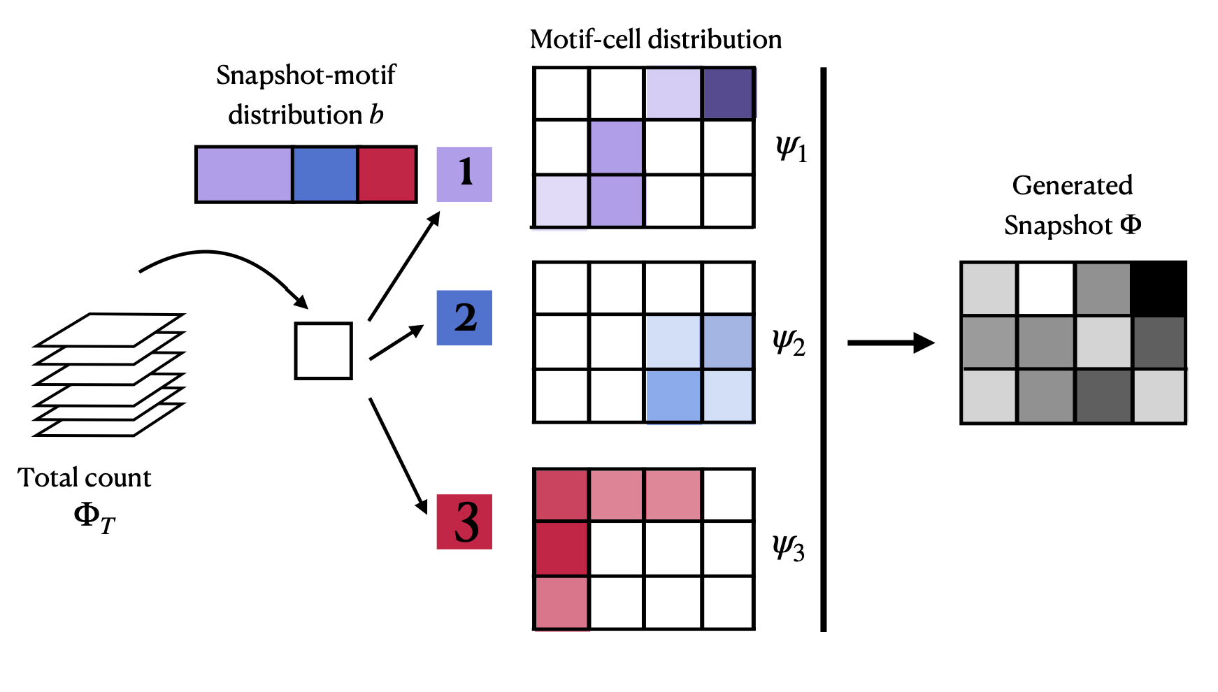
In Fluid Mechanics applications ([29, 32]), sampling from the motif-cell distribution (step c)) can be replaced with a faster step, where the contribution of each motif to snapshot is directly obtained from the motif-cell distribution and the distribution and expressed as . The reconstructed field is then the sum of the motif contributions. Figure 3 illustrates the LDA generative process on a grid for three topics.
IV.4 Interpretation and evaluation criteria
By construction, the decomposition identifies fixed regions of space over which the intensity of the scalar field is likely to be important at the same time. The connection between temperature motifs and plumes should be examined with caution since plumes are Lagrangian structures travelling and possibly changing in shape and orientation through the shell. LDA motifs only aim to detect the Eulerian signature of structures.
Each motif can be characterized in space through the motif-cell distribution (which integrates to 1 over the cells) and which will sometimes referred to as the motif in the absence of ambiguity. Each distribution has a maximum value and a maximum location such that . One can also define a characteristic area using
| (9) |
where represents the plane of analysis and the factor is an arbitrary factor chosen by analogy with a Gaussian distribution. Characteristic dimensions for the motif in the direction can also be defined using . Each motif can also be characterized in time through the snapshot-motif distribution , that will be called the motif weight throughout the paper. The motifs can be ordered by their time-averaged weight, also called prevalence, defined as where represents a time average.
LDA decompositions were carried out independently for the heat flux , temperature fluctuations and the total kinetic energy . To differentiate between these quantities, the motif topics and weights will be denoted respectively as , and and , and . A useful tool for comparing the motifs associated with two different quantities is to compute the correlation coefficient matrix between the corresponding motif weights (for instance if we compare the heat flux and the temperature motifs, each entry of the matrix will correspond to the correlation coefficient between and ).
As noted above, a reconstruction of the field can be obtained by using the inferred motif-cell distribution and snapshot-motif distribution to provide what we will call the LDA-Reconstructed field, defined as
| (10) |
where represents the sum of the field values over the cells. To evaluate the relevance of the decomposition, one can compute for each snapshot the instantaneous spatial correlation coefficient between a given field and its reconstruction defined as
| (11) |
where represents the fluctuation A global measure of the reconstruction is then given by , the average value of over all snapshots.
V Evaluation of LDA for reconstruction and generation of the heat flux
V.1 Reconstruction
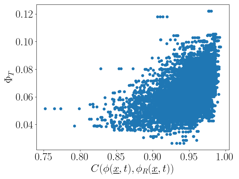
We first evaluate to which extent the LDA decomposition provides an adequate reconstruction of the heat flux . Figure 4 (left) shows how the instantaneous value of the correlation coefficient depends on the discrete integral of the field . The Rayleigh considered is and the number of topics is , but the same trend was observed for all other Rayleigh numbers as well as all other values of . Lower values of the correlation were associated with lower values of the total integrated heat flux, which illustrates that the LDA representation is suited to capture extreme events.
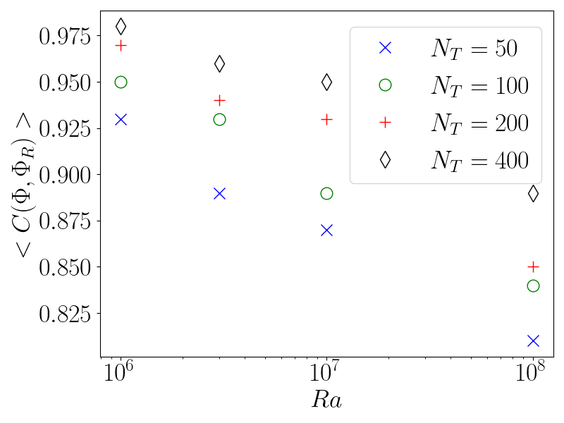
Figure 4 (right) presents the mean correlation coefficient for different number of motifs and different Rayleigh numbers on the vertical planes. Unsurprisingly, the correlation increases with the number of topics. It also decreases with the Rayleigh number, which is consistent with an increase in the complexity of the flow. However, the minimum value for the lower number of topics and the highest Rayleigh number was 0.8, which shows the relevance of the decomposition.
Figure 5 compares an original snapshot at (based on the digitized signal) with different reconstructions: i) the LDA-reconstruction based on motifs, ii) the reconstruction limited to the 20 most prevalent topics (for this particular snapshot), iii) the POD-based reconstruction based on the first 20 modes. By construction, POD provides the best approximation of the field for a given number of modes. Since the distribution of the heat flux is intermittent in space and time, only a limited number of motifs is necesssary to reconstruct the flow. We note that little difference was observed between the full LDA reconstruction and the reconstruction limited to the 20 most prevalent motifs, which highlights the intermittent nature of the field. The relative error between the original and the reconstructed field is 29% for the full LDA reconstruction, 34 % when the 20 most prevalent modes are retained in the reconstruction. In contrast, limiting the POD to 20 global modes slightly lowers the quality of the reconstruction, with a global error of 38%. It should be noted that the 20 dominant POD modes correspond to an average over all snapshots, while the 20 most prevalent LDA modes are selected for that specific snapshot. On average, the reconstructed field based on keeping the 20 most prevalent motifs differed by less than 10% from the full 100-mode reconstruction and the average correlation coefficient decreased from 0.89 to 0.83. This shows that LDA can provide a compact representation of the local heat flux that compares reasonably well with POD.
V.2 Generation
The ability to generate statistically relevant synthetic fields is of interest for a number of applications, such as accelerating computations or developing multi-physics models. As a generative model, LDA makes it possible to produce such a set of fields, the statistics of which can be compared with those of the original fields used to extract the motifs, as well as with those of the corresponding LDA-Reconstructed fields. It would also be useful to compare the generated LDA data set with one generated using POD. To this end, we generated two sets of 4000 new fields using both LDA and POD. The same number of POD modes and LDA motifs were used to generate the datasets. The plane in which the data is generated is assumed to be the plane. The different fields to be compared are therefore the following:
- 1.
-
2.
the LDA-Reconstructed field (LDA-R) as defined in equation (10)
-
3.
the LDA-Generated field (LDA-G): the field is constructed by sampling weights from snapshot-motif distributions and then reconstructing
(12) where is a random variable obtained by sampling a Poisson distribution with the same statistics as the original database.
-
4.
the POD-Generated field (POD-G): the field is constructed by independently sampling POD mode amplitudes from the POD amplitudes of the original database
(13)
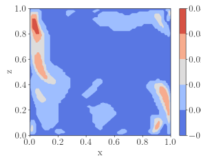
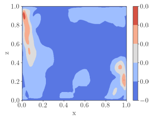
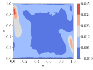
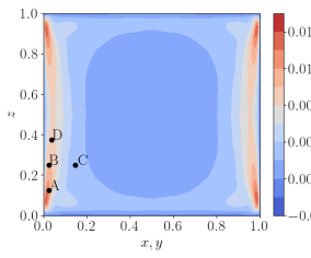
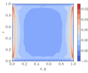
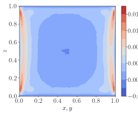
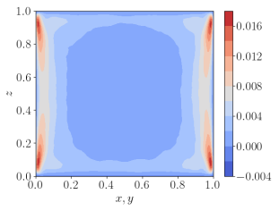
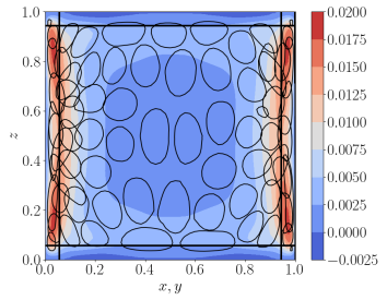
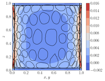
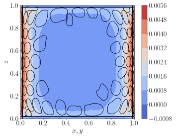
The time-averaged fields corresponding to the different databases are compared in Figure 6. A good agreement is observed for all datasets, with global errors of 4%, 8% and 3% for respectively the LDA-reconstructed, the LDA-generated and the POD-generated datasets. Although it provides the lowest error (as could be expected), the POD-generated data set overestimates negative values in the core of the cell.
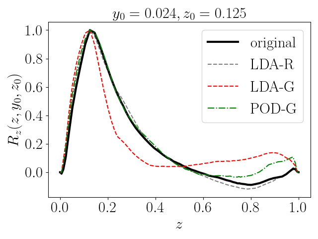
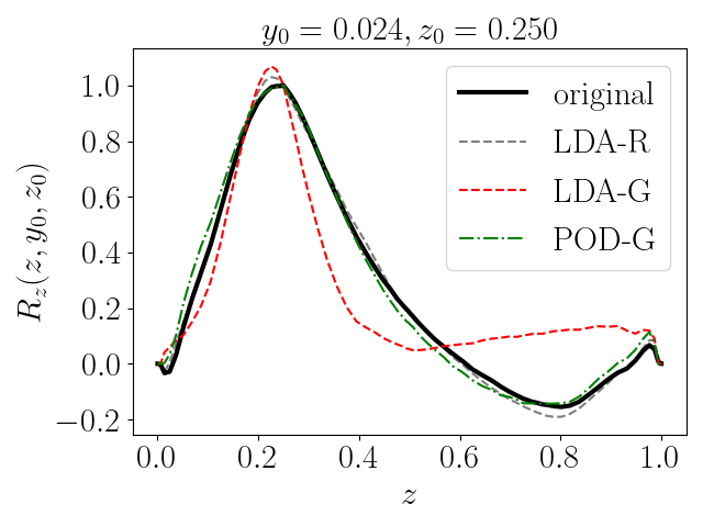
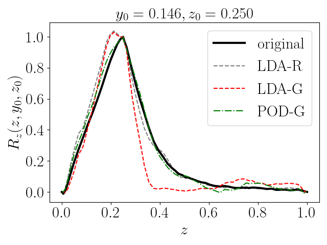
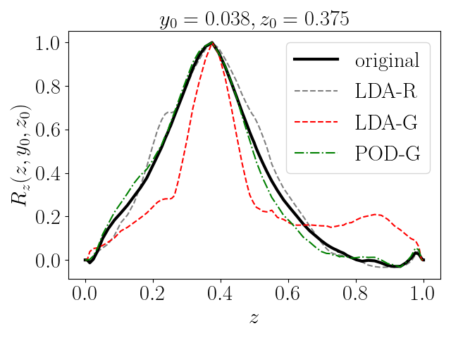
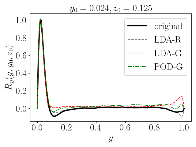
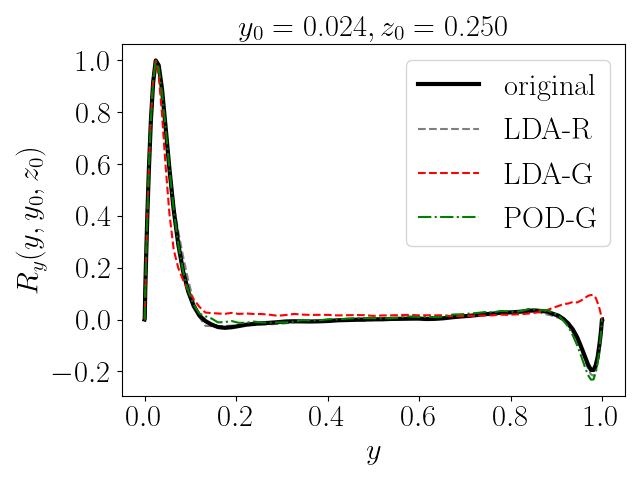
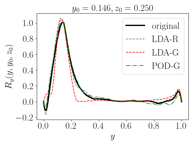
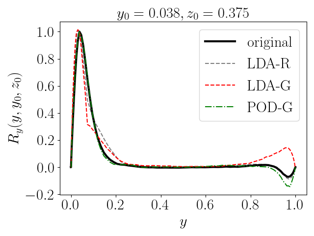
For a given location , we defined spatial autocorrelation functions in the horizontal and vertical directions as:
| (14) |
| (15) |
The autocorrelation functions are displayed in Figure 7 for the selected locations indicated in Figure 6, which correspond to regions of high heat flux. We can see that that in all cases, the flux remains correlated over much longer vertical extents than in the horizontal direction. Both the LDA-reconstructed and the POD-generated autocorrelations approximate the original data well - again, by construction, POD-based fields are optimal to reconstruct second-order statistics. The LDA-generated autocorrelation is not as close to the original one, but still manages to capture the characteristic spatial scale over which the fields are correlated.
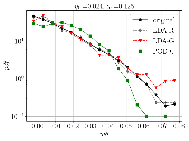
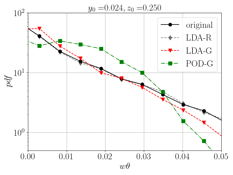
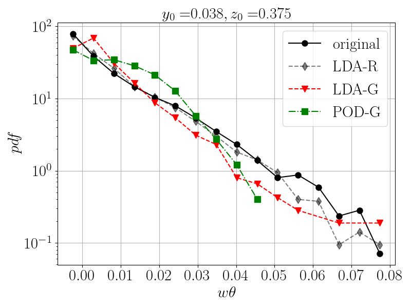
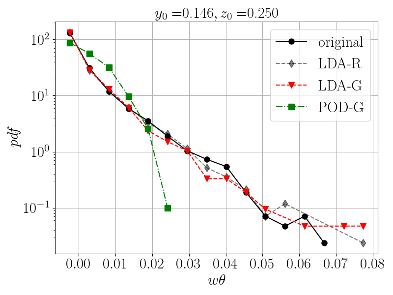
One-point pdfs of the flux are represented in Figure 8 for the same selected locations (again, indicated in Figure 6). POD-generated fields tend to overpredict lower values and underpredict higher values, which means that they do not capture well the intermittent features of the heat flux. The LDA-generated fields display a better agreement with the original fields and are in particular able to reproduce the exponential tails of the distributions.
VI Heat flux motifs
VI.1 Spatial organization
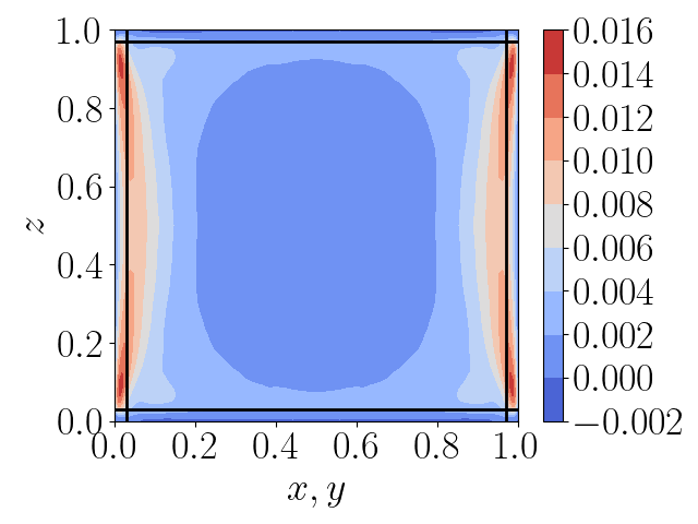
We now describe the spatial organization of the motifs through the motif-cell distribution . The general trends reported below held for all values of considered, which ranged from 50 to 400. For all Rayleigh numbers, most LDA motifs were found to be associated with a positive flux (i.e were associated with the first cells in the decomposition). A few negative (counter-gradient) motifs were also identified, but their average weight was generally very small (at most 10 % of that of the dominant motif). We therefore chose to focus only on the motifs with a positive contribution to the heat flux. Figure 9 (left) displays these motifs for three different Rayleigh numbers for . The case was omitted as it did not show significant differences with the case . The motif-cell distribution is materialized by a black line corresponding to the iso-probability contour of , which can be compared with the average value of the heat flux at this location. For all Rayleigh numbers, the motifs are clustered in the regions of high heat flux, close to the vertical walls. Within the vertical boundary layers, motifs are elongated in shape. Outside the vertical boundary layers, the motifs are more isotropic and tend to increase in shape as one moves away from the walls. Outside the horizontal boundary layers, the motif-cell distributions are elongated in the direction of the wind, with a horizontal orientation in the center of the cell, and a gradual vertical shift closer to the walls. Large motifs are found in the bulk at and (it was also the case at ). In contrast, fewer, smaller motifs are found in the bulk at in the central region , signalling a loss of spatial coherence in the bulk at this Rayleigh number.
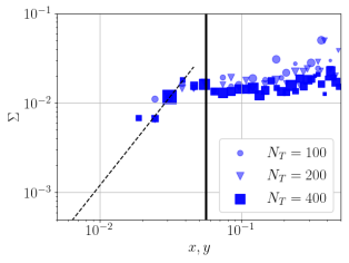
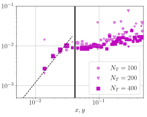
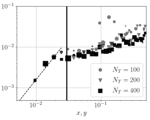
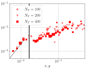
In general, the motif size seems to decrease with the Rayleigh number. This is confirmed by Figure 10, which represents the average motif area as a function of their distance from the vertical walls. In order to avoid the influence of the horizontal plates, we only considered the motifs located at a vertical distance larger than from the horizontal walls (i.e. outside the horizontal boundary layer). The size of the symbols shown in the picture is proportional to the fraction of motifs over which the average was performed. Results were relatively robust with respect to the number of topics , although some dependence on is observed in the center of the cell. Within the boundary layer, the motif area grows quadratically, which means that the characteristic size of the motif is proportional to the wall distance. We note that a similar scaling was found for turbulent eddies in pressure-gradient driven turbulence such as channel flow [29]. Further away from the vertical wall, after a short plateau at the edge of the boundary layer, a slower increase in the motif size was observed with a rate that increased with the Rayleigh number, so that the motif area was about the same (on the order of ) for all Rayleigh numbers in the center of the cell. This suggests the presence of a double scaling for the motifs: one based on the boundary layer thickness, and one based on the cell size. The decrease in size with the Rayleigh number appears consistent with a dependence on the boundary layer thickness but also with an increase of the fragmentation by the bulk turbulent fluctuations, in agreement with the literature [6, 15]. The difference observed at the highest Rayleigh number also signals that the flow is still evolving and has not reached an asymptotic state.
VI.2 Dominant motifs
VI.2.1 Spatial description
Owing to the symmetry of the database, the motifs in the vertical plane (resp. ) should approximate the symmetry (resp. ), and (complete symmetry cannot be expected owing to the stochastic nature of the decomposition).
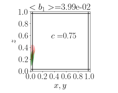
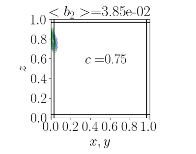
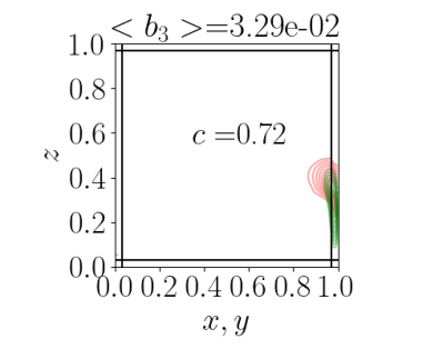
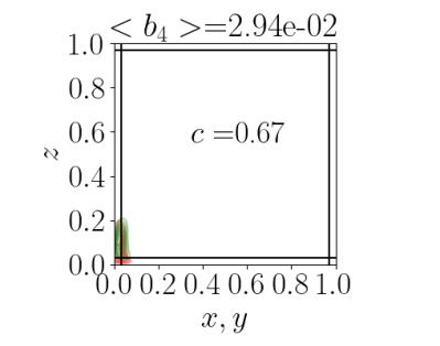
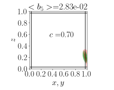
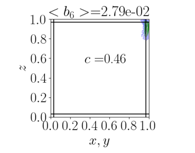
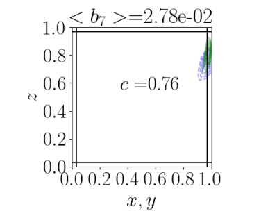
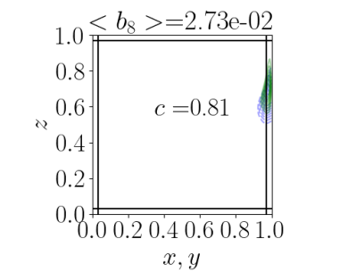
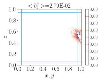
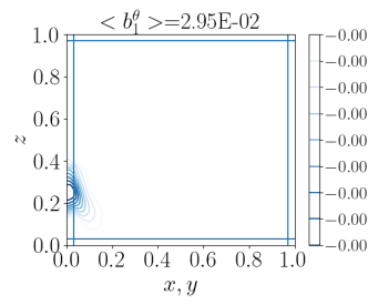
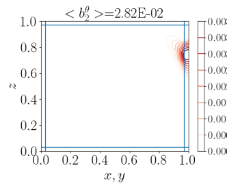
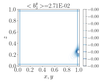
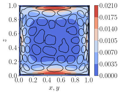
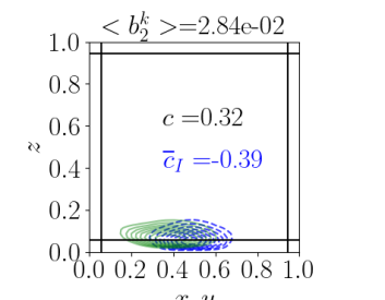
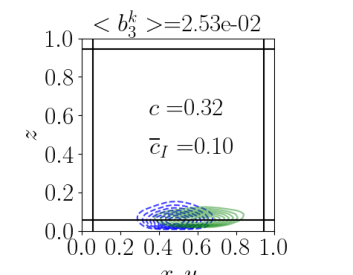
To help interpret the heat flux motifs, we compare them with LDA motifs corresponding to temperature fluctuations. The eight most prevalent heat motifs are represented in figure 11 (green lines). The prevalence of each motif is indicated at the top of each plot. Most motifs have similar sizes and are located close to the side walls at about a similar height, except for motifs 4 and 6, which have a smaller extent and are located closer to the horizontal wall. The same value of was used for both heat flux and temperature.
For a heat flux motif with weight , we identified the temperature motif that maximized the correlation coefficient between the heat flux and the temperature motif weights .
The maximal value of this coefficient, denoted , is represented on each plot and is generally very high (about 0.7) - especially in view of the intermittent nature of the weights. The best correlated heat flux and temperature motifs are close to each other in space, with a larger spread for temperature motifs. In all cases, flux motifs in the lower (resp. higher) portion of the side walls correspond to positive (resp. negative) fluctuations. Dominant heat flux motifs can be therefore interpreted as the wall imprint of hot plumes rising in the boundary layer (resp. cold plumes descending in the boundary layer). The same observations were made at all other Rayleigh numbers.
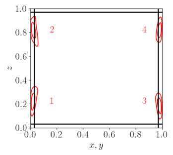
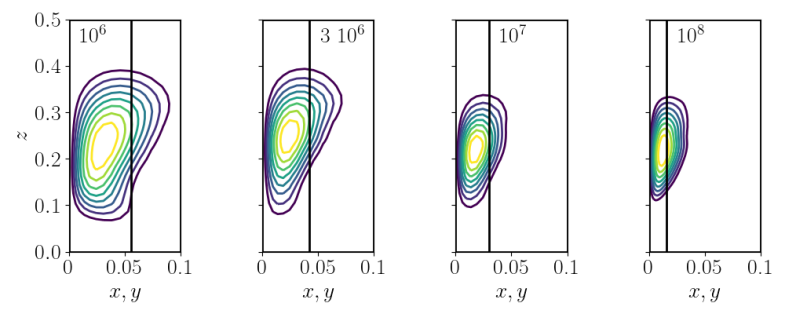
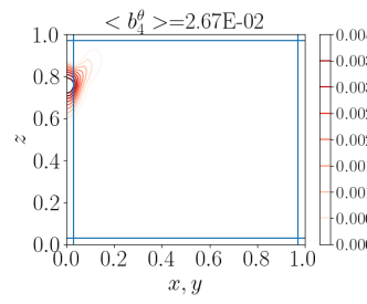
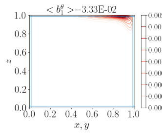
Four of these dominant motifs at are represented in Figure 12 (left) for . As noted above, they consist of elongated structures lying mostly in the boundary layer, and located at a vertical distance of about 0.25 from the horizontal walls. Although the positions and sizes of the four identified motifs may slightly vary from one to the other, their features are generally similar and a characteristic motif can be obtained from taking the average over all four motifs. Figure 12 (right) represents this characteristic motif for the various Rayleigh numbers. We can see that the dominant motifs are always located mostly within the boundary layer, with a maximum at a height of about . Their characteristic width was found to decrease as , which matches the scaling of the boundary layer thickness.
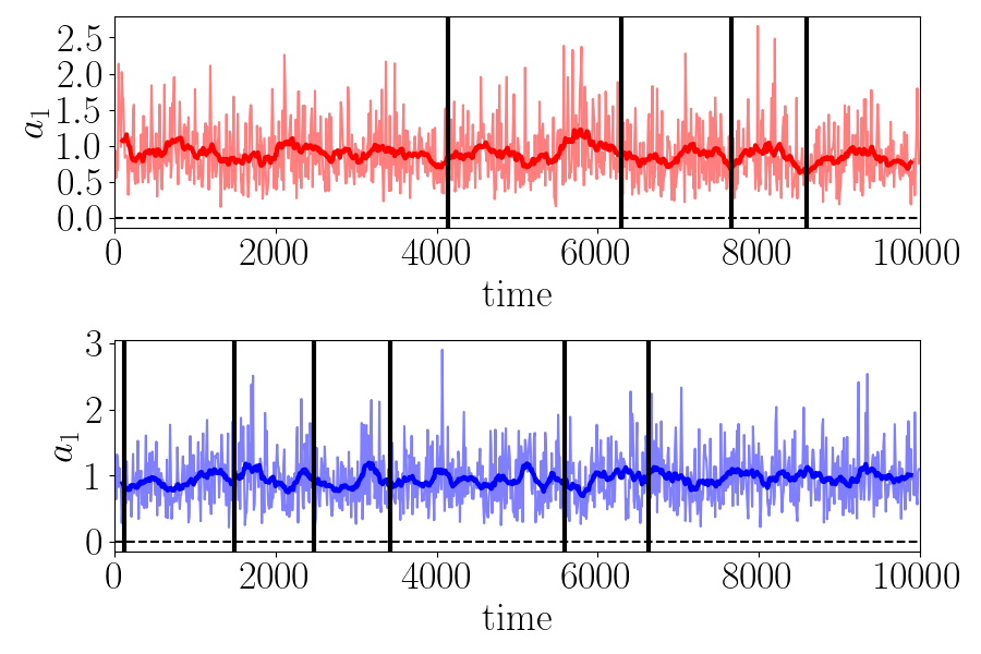
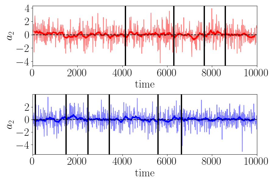
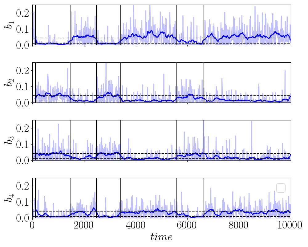
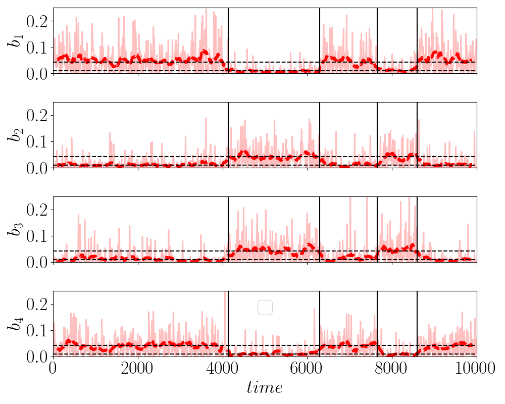
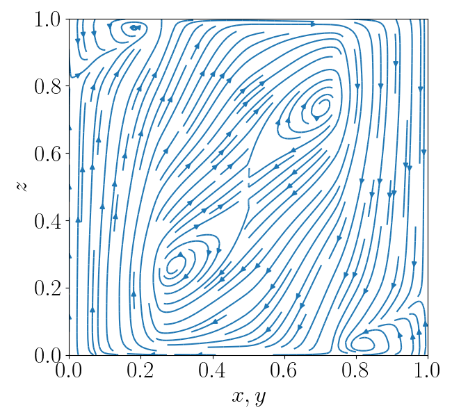
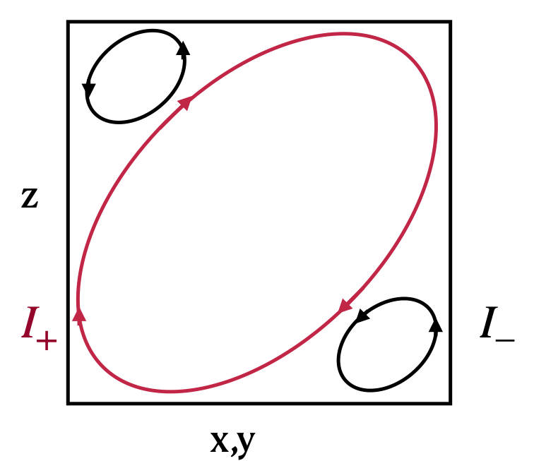
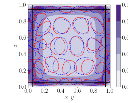
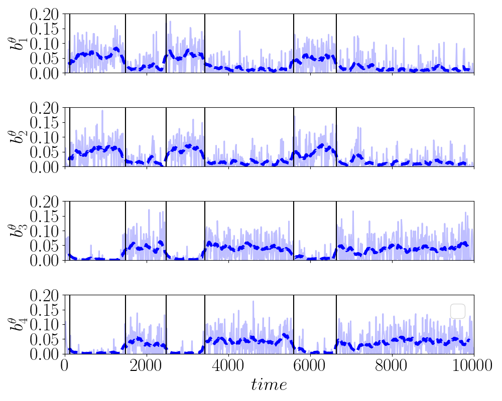
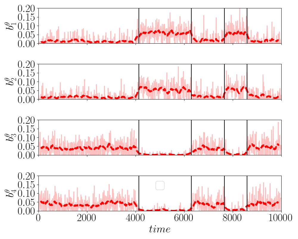
The evolution of the snapshot-motif distribution, or motif weight, is represented in Figure 13 for . We can see that the behavior of the motif weight depends on the sign of the global momentum represented in Figure 1. When a moving average of time units, corresponding to 4 recirculation times , was applied, two quasi-stationary states and could be identified in each plane - they are materialized by the dashed horizontal black lines indicated in Figure 13. The two states appear to correspond to the sign of the angular momentum component i.e. the orientation of the large-scale circulation . Streamlines of the flow conditionally averaged on the higher weight value of are represented in figure 14 left). They indicate that for the higher characteristic value of the weight, , the motif is associated with the large-scale circulation while it is associated with the corner vortex on the opposite side for the lower weight value, , as summarized in figure 14 right).
This indicates that information about the large-scale reorientation can be extracted from local measurements. Two states, and , respectively corresponding to the large-scale circulation and corner vortex can be defined from the weight of the dominant motif using
| (16) |
where represents the moving average over . The average weights conditioned on and are respectively and .
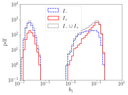
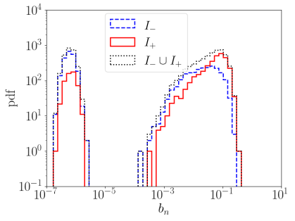
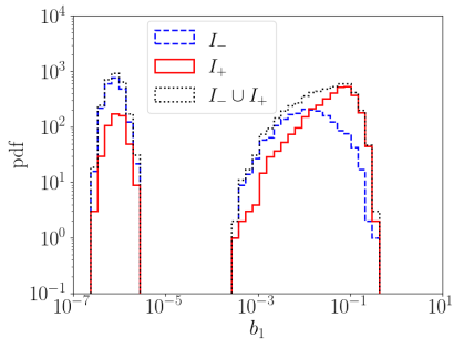
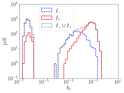
Figure 15 displays the histogram of the weight of the dominant motif (motifs 2 to 4 displayed similar features). At all Rayleigh numbers, the total distribution is characterized by two distinct lobes, which correspond to the absence and the presence of the motif in the snapshot. The relative importance of the lobes therefore provides an indirect measure of the motif intermittency, which can be related to plume emission. The ratio of motif presence to motif absence was about 0.5-0.6 in the range of Rayleigh numbers considered - no significant variation was observed with the Rayleigh number.
However, further insights can be obtained by examining the respective contributions of the and states to the distribution of , which are also represented in Figure 15. For all Rayleigh numbers, states contribute more to the higher-value lobe than states, while contributes more to the lower-value lobe. This shows that the rate of buoyancy production is less intense in the corner rolls than in the large-scale circulation, or equivalently that plumes are emitted at a lower frequency in the corner rolls than in the large-scale circulation. Moreover, the relative contributions of the and the states vary non-monotonically with the Rayleigh number. In the higher-value lobe, the relative contribution of appears to increase relatively to with more high values of at , while represents more low values at . In the lower-value lobe, the contribution of is least at and largest at . These observations suggest that both the intensity of the large-scale circulation and that of the corner roll appear to change with the Rayleigh number, in agreement with the findings of Vishnu et al. [39].
VI.2.2 A model for the reorientation time scale
A simple model can be made to link these observations with the dynamics of reorientations. The conditionally averaged weight of the dominant motif in the region close to the wall represents the rate of buoyancy production, which can be linked to the emission rate of plumes and can be modelled as a Poisson point process. This means that the time separating two plume ejections follows an exponential distribution with mean , where and respectively characterize the large-scale circulation () and the corner vortex () states. therefore represents the parameter of the exponential distribution. A reorientation can be associated with the event where the corner vortex becomes stronger than the large-scale circulation state, i.e. the time separating two emissions in the corner vortex state becomes smaller than that separating two emissions in the large-scale circulation state. This event can occur independently in either one of the two horizontal directions or .
One can show that the probability that this event occurs at any given time is given by
| (17) |
Owing to the memoryless nature of the exponential distribution, this holds for the time separating an arbitrary number of emissions, in particular over a characteristic time sufficiently long to reverse the circulation in that direction. should be on the order of the recirculation time so that we have with . If is the recirculation frequency, one would then expect the frequency between reorientations to depend on and following
| (18) |
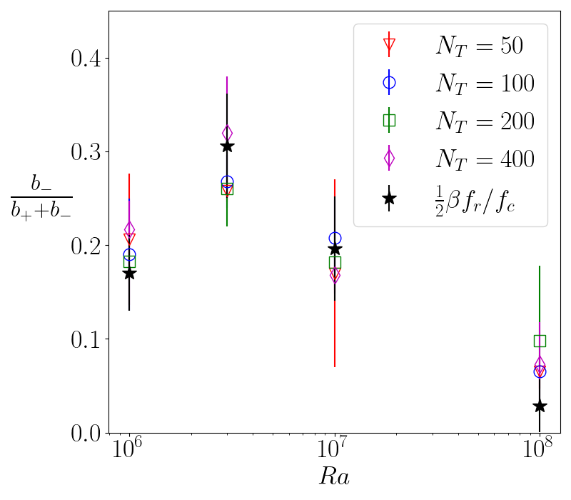
where the factor comes from the fact that a reorientation can occur in each direction. Figure 16 (right) compares for different Rayleigh numbers the probability with the ratio of the frequency between reorientations and the recirculation frequency estimated in [26]. We see that a very good agreement is obtained between the variations of the average reorientation rate and the measure of the relative intensity of the large-scale circulation and corner vortices. We note that the largest discrepancy is observed for the highest Rayleigh number, for which the reorientation rate is very low and therefore cannot be determined with good precision from the DNS. The value of used in the figure was determined empirically and was found to be , which makes close to the filtering time scale . This suggests that an estimate for the reorientation rate can be obtained by comparing directly the average weight of the motif associated with the large-scale circulation with that of its counterpart in the corner structure. This could be of particular interest in cases where the observation time is smaller than the expected reorientation time, a situation that is often encountered in - but not limited to - numerical simulations.
VII Temperature and velocity motifs
In this section we try to understand the physics associated with the lower reorientation rate observed as the Rayleigh number increases. For this we turn to temperature and velocity fluctuations, to which we independently applied LDA. Although these are not intermittent quantities, and therefore might not be considered a priori appropriate for LDA application, table 2 shows that the temperature and kinetic energy fields are relatively well reconstructed.
| Ra= | |||||
|---|---|---|---|---|---|
| 100 | 0.90 | 0.86 | 0.84 | 0.66 | |
| 400 | 0.94 | 0.92 | 0.90 | 0.78 | |
| 100 | 0.91 | 0.88 | 0.85 | 0.78 | |
| 400 | 0.94 | 0.92 | 0.89 | 0.82 | |
| 100 | 0.96 | 0.93 | 0.89 | 0.84 | |
| 400 | 0.98 | 0.96 | 0.95 | 0.89 |
VII.1 Temperature fluctuations
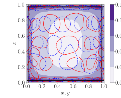
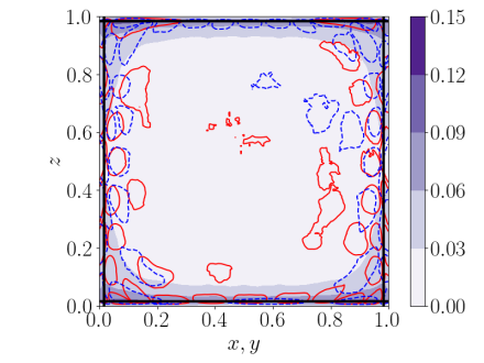
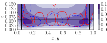
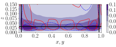
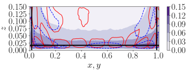
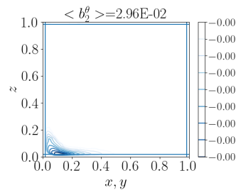
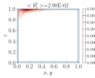
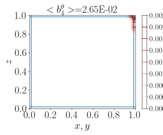
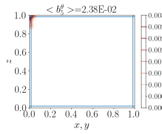
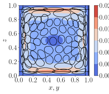
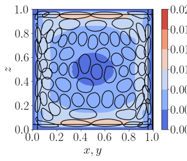
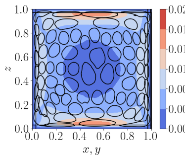
Figure 17 shows the temperature motifs at three different Rayleigh numbers, along with the variance of the fluctuations, for . As mentioned above, some symmetry is expected but not perfectly enforced, due to the statistical character of the method. As for heat flux motifs there is a clear difference between the boundary layers and the bulk, as well as a strong decrease of motifs in the central part of the cell at . We can see that temperature fluctuations are also important close to the horizontal walls. The bottom row of figure 17 shows a close-up of the lower part of the cell. The maximum of the motif spatial distribution is located at the edge of the boundary layer. The height of the motifs scale with the boundary layer height in the center of the cell, with negative motifs shorter and wider than positive ones in the bottom layer. Analogous observations can be made for the top wall, by swapping the role of cold and hot fluctuations.
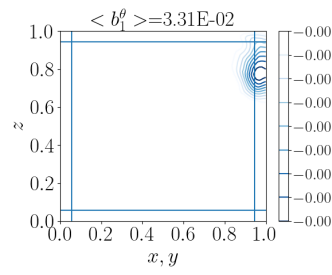
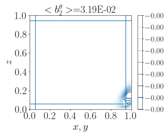
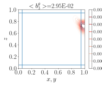
Figure 18 represents the first four dominant motifs for the temperature at (similar observations can be made at ). Although the most likely heat flux motifs corresponded to hot plumes near the bottom wall and cold plumes near the top wall, this is not the case for the temperature motifs. For the two lower Rayleigh numbers, temperature motifs are as likely to be found near the bottom wall than near the top wall. However, at , figure 19 shows that the most likely temperature motifs correspond to hot fluctuations along the bottom side walls and cold near the top side wall, corresponding to late-stage plumes arriving at the opposite wall.
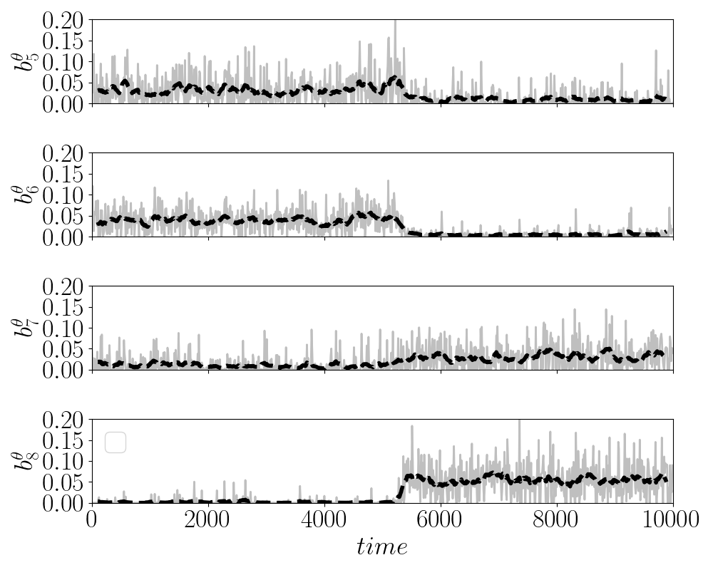
Figure 20 shows the evolution of the temperature motif weights on both planes along the filtered representation (i.e. corresponding to an average of . ). As observed for the heat flux (figure 13), the importance of the weights depends on the orientation of the large-scale circulation . Similar evolutions were observed at the lower Rayleigh numbers (not shown).
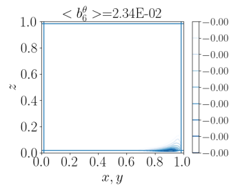
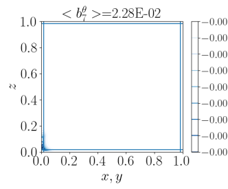
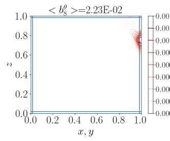
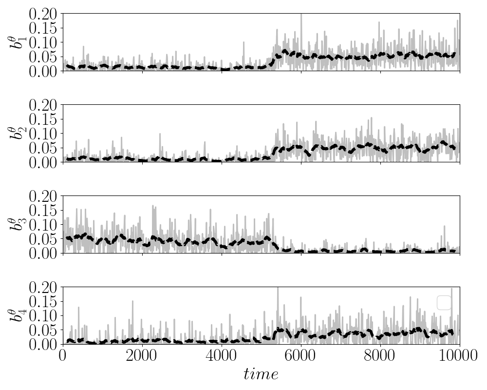
Strong differences can be observed when comparing figures 19 and 21. At , the most likely temperature motifs are no longer located within the vertical boundary layers, but extend from the corner of the cell along the horizontal walls. The first eight dominant structures consist of two types of corner motifs: large, predominantly horizontal ones, and small, vertical ones located within the boundary layers. Motifs near the top (resp. bottom) wall are hot (resp. cold) and therefore correspond to late-stage plumes. This is confirmed by the evolution of the motif weights shown in figure 22 for the plane . These motifs correspond to hot fluid being brought from the bottom layer by the large-scale circulation next to the top wall and into the corner structure, thus decreasing buoyancy effects there. These observations are consistent with the reduction in intensity of the corner roll and the significant decrease in the reorientation rate observed at this Rayleigh number. We note that although the small vertical temperature motifs are similar to the heat flux motifs 4 and 6 identified in figure 19 at , they represent fluctuations of the opposite sign, and they are well correlated (or anti-correlated) with the orientation of the large-scale circulation. This confirms the dominance of the impinging plumes in the corners of the cell.
VII.2 Kinetic energy
More details about the structure of the large-scale circulation can be obtained by examining kinetic energy motifs. Figure 23 shows the spatial distribution of the velocity motifs for the different Rayleigh numbers and . The spatial distribution of the time-averaged kinetic energy is also represented on the same plot. The size of the core (low-velocity region) appears to increase with the Rayleigh number. The size of the motifs did not appear to change significantly with the Rayleigh number, except for horizontal corner structures that seem to scale with the boundary layer thickness. The kinetic energy motifs have elongated shapes along the walls, with a significantly higher extent along the horizontal walls, which shows the importance of entrainment in the horizontal boundary layers, in particular in the middle of the cell. It is lowest at and highest at , which varies like the time between reorientations . The question is whether this reinforcement of the large-scale circulation can be associated with characteristic temperature fluctuations.
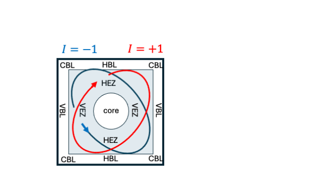
In figures 24 to 26 the 16 most prevalent kinetic energy motifs are represented at Rayleigh numbers , and (the case , not shown, was found generally similar to and ). The motifs were organized according to the location of their maximum: within the horizontal or vertical boundary layers, which we will refer to as respectively HBL or VBL motifs, at the corners of the horizontal and the vertical boundary layer (CBL motifs), and outside the boundary layers in the horizontal or vertical entrainment zones, which were termed HEZ or VEZ motifs. The different locations are shown in the top right illustration of figure 24. For each category the motifs are ordered according to their prevalence, indicated at the top of each plot. Generally speaking, the prevalence of the motifs increased with the Rayleigh number, which is consistent with a strengthening of the large-scale circulation.
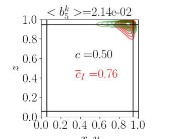
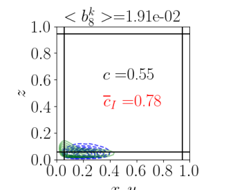
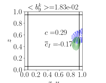
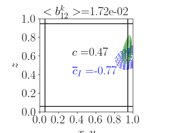
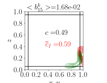
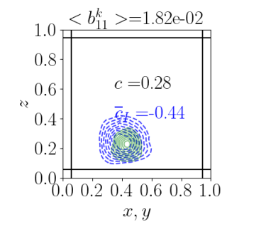
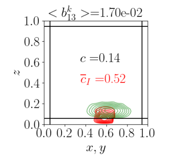
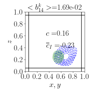
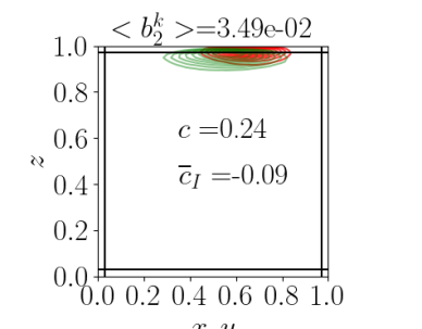
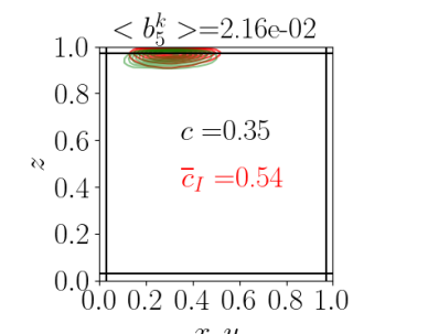
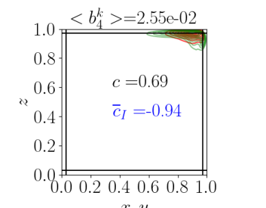
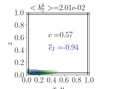
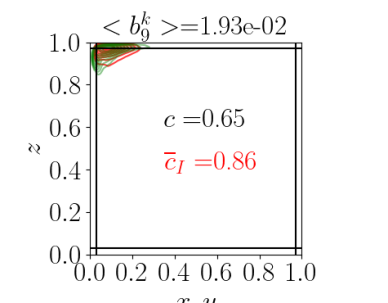
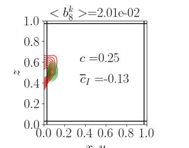
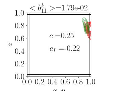
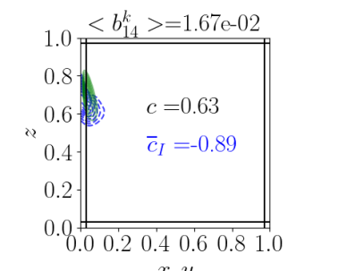
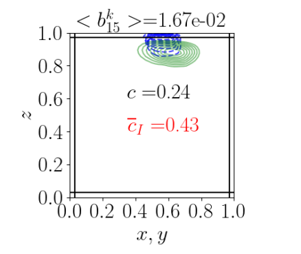
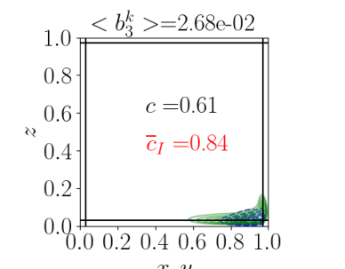
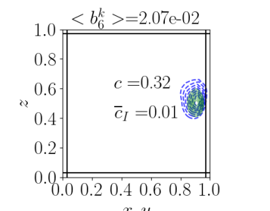
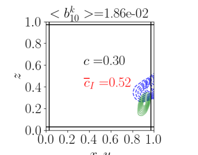
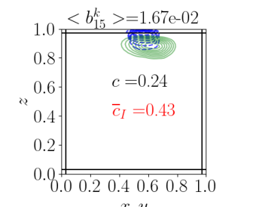
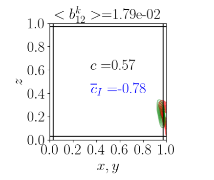
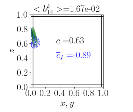
For each kinetic energy motif (represented with green lines), we determined the temperature motif (represented with blue or red lines, depending on its sign) for which the correlation coefficient is maximal. The maximal value and the temperature motif are represented on each plot, except in two cases corresponding to HBL motifs, for which the associated temperature motif had a very low prevalence and was considered to be irrelevant. In almost all cases, the kinetic energy and temperature motifs are located close to each other in space. Although the correlation coefficients are typically lower than those between the flux and temperature motifs represented in figure 11, several are high enough to associate kinetic energy patterns with specific temperature fluctuations. We also represented on each plot the correlation coefficient , defined as , where is the low-pass-filtered kinetic energy motif weight (using ) and is the large-scale circulation indicator defined in section II B (see also figure 24 top right). High positive (resp. negative) values of are indicated in red (resp. blue) for each motif, and show that the motif can be associated with a specific orientation of the large-scale circulation.
In all cases, the most frequent motifs consist of centered motifs close to the edge of the horizontal boundary layers (HBL). Evidence of weak correlation (0.3) for some motifs suggested possible association with impinging plumes, however generally low values of suggest that the weights of the motifs do not depend on the orientation of the large-scale circulation. In contrast, high values of and were found for corner (CBL) motifs, that were best correlated with impinging plumes. Corner motifs have a relatively high prevalence, which shows that impinging plumes make a significant contribution to the horizontal wind at the edge of the boundary layer. The correlation coefficient increased in absolute value with the Rayleigh number, and was larger than 0.9 at . In contrast, the maximum correlation coefficient tended to decrease (but remained significant) at .
The next prevalent category of motifs at and consisted of motifs in the vertical entrainment zone (VEZ motifs). They were generally weakly correlated with temperature motifs of a slightly larger size ( and were still less correlated with the orientation of the large-scale circulation ( close to zero), which is consistent with their mid-height location. Two of the motifs at (third and fourth motifs) were located closer to a horizontal wall and showed a stronger correlation with . They were found to be correlated with ”upstream” temperature fluctuations originating from the opposite wall (arriving plumes). At , only one VEZ motif, with a lower prevalence (compared with the other motifs), was identified. It also corresponded to an arriving plume and was strongly correlated with the orientation of the large-scale circulation.
High values of were also observed for motifs within the vertical boundary layers (VBL), as well as significant values of . The corresponding temperature motifs were also located within the vertical boundary layers and consisted of hot (resp. cold) temperature fluctuations close to the bottom (resp. top plate), suggesting that they correspond to plumes in the early formation stage (leaving plumes).
At and , the last category of motifs consisted of motifs in the horizontal entrainment zone (HEZ). At the lowest Rayleigh number , two of the HEZ motifs (second and fourth motif in the last row in figures 24) have a predominantly vertical shape and are associated with large temperature motifs originating from the opposite (here, top) wall. They are therefore likely to represent coalescing plumes drifting towards the center of the cell as they reach the opposite wall. In contrast, all other HEZ motifs at all Rayleigh numbers have a horizontal shape and are associated with smaller temperature motifs originating from the closest wall. They are very well correlated with the orientation of the large-scale circulation. Significant changes were observed at , with a much larger number of HEZ motifs and a noticeable increase in their prevalence - the prevalence of the dominant HEZ motif is twice as large at than at .
To sum up, a significant difference is observed between and . At the highest Rayleigh number, the large-scale circulation is largely reinforced in the horizontal direction due to the formation of new plumes, while stronger impinging plumes remain confined to the corner boundary layers.
VIII Conclusion
We have applied a new analysis technique, Latent Dirichlet Allocation, to characterize the spatio-temporal organization of fluctuations in Rayleigh-Bénard convection. The method is based on the inference of probabilistic latent factors, spatially localized motifs, from a collection of instantaneous fields. It provides a local yet compact description of the flow in terms of quantitative indicators such as the (spatial) size and the (temporal) weight of the motifs. The technique was applied to the vertical mid-plane of a Rayleigh-Bénard cubic cell in a range of Rayleigh numbers in . The method was found to be robust with respect to the user-defined parameters. When applied to the heat flux, it was found to provide good reconstructions of the snapshots and was able to generate new datasets that reproduced key statistics of the original one.
For all Rayleigh numbers, dominant heat flux motifs consisted of elongated vertical structures located mostly within the vertical boundary layer, at a height of a quarter of the cell. The width of these motifs scaled with the boundary layer thickness. These motifs were found to be very well correlated with temperature motifs corresponding to plumes in their early formation stage (leaving plumes). The motif weights were found to depend on the large-scale organization of the flow: two states could be identified - one corresponding to the large-scale circulation and one to a corner roll structure. The two states were characterized by different average weights which varied non-monotonically with the Rayleigh number. A simple model was able to relate the weights of the dominant heat flux motif associated with the two states with the average reorientation rate of the large-scale circulation in the cell. This suggests that the model could be used as a predictor of this rate in cases where few or even no reorientations are observed.
Additional insight about the flow physics was obtained by examining dominant motifs for the temperature and the kinetic energy. While dominant heat flux motifs seemed to be associated with early-stage (leaving) plumes, dominant temperature motifs were associated with later-stage (arriving) plumes. In contrast with the lower Rayleigh numbers, dominant temperature motifs at were no longer within the vertical boundary layers, but consisted of plumes impinging onto the corners of the horizontal boundary layers, which led to a reduction of temperature gradients within the corner structure and a decrease in its potential energy. This is consistent with the significant drop in the large-scale reorientation rate observed at this Rayleigh number. LDA analysis of the kinetic energy showed that corner impinging plumes contributed to the kinetic energy of both the corner structure and the large-scale circulation. The reduction of the reorientation rate at was also associated with a reinforcement of the horizontal wind in the central part of the cell due to the formation and entrainment of new plumes. The LDA model therefore appears as a promising statistical tool that can help track subtle transitions in the dynamics of turbulent flows.
Acknowledgements.
This work was granted access to the HPC resources of IDRIS under the allocation 2023- AD012A62062R1 made by GENCI. We thank Anouar Soufiani and Philippe Rivière for helpful discussions about the manuscript. We are also grateful to Jean-Michel Dupays, Rémy Dubois and Camille Parisel for technical support and helpful discussions.References
- Grossmann and Lohse [2000] S. Grossmann and D. Lohse, Scaling in thermal convection: a unifying theory, Journal of Fluid Mechanics 407, 27–56 (2000).
- Grossmann and Lohse [2004] S. Grossmann and D. Lohse, Fluctuations in turbulent rayleigh-benard convection: The role of plumes, PHYSICS OF FLUIDS 16, 4462 (2004).
- Xi et al. [2004] H.-D. Xi, S. Lam, and K. Xia, From laminar plumes to organized flows: the onset of large-scale circulation in turbulent thermal convection, Journal of Fluid Mechanics 503, 47–56 (2004).
- Castaing et al. [1989] B. Castaing, G. Gunaratne, F. Heslot, L. Kadanoff, A. Libchaber, S. Thomae, X.-Z. Wu, S. Zaleski, and G. Zanetti, Scaling of hard thermal turbulence in Rayleigh-Bénard convection, Journal of Fluid Mechanics 204, 1 (1989).
- Wang et al. [2022] Y. Wang, Y. Wei, P. Tong, and X. He, Collective effect of thermal plumes on temperature fluctuations in a closed rayleigh–bénard convection cell, Journal of Fluid Mechanics 934, A13 (2022).
- Bosbach et al. [2012] J. Bosbach, S. Weiss, and G. Ahlers, Plume fragmentation by bulk interactions in turbulent rayleigh-bénard convection, Phys. Rev. Lett. 108, 054501 (2012).
- Shang et al. [2003] X.-D. Shang, X.-L. Qiu, P. Tong, and K.-Q. Xia, Measured local heat transport in turbulent rayleigh-bénard convection, Phys. Rev. Lett. 90, 074501 (2003).
- Zhou et al. [2007] Q. Zhou, C. Sun, and K.-Q. Xia, Morphological evolution of thermal plumes in turbulent rayleigh-benard convection, PHYSICAL REVIEW LETTERS 98, 10.1103/PhysRevLett.98.074501 (2007).
- Shishkina and Wagner [2008] O. Shishkina and C. Wagner, Analysis of sheet-like thermal plumes in turbulent rayleigh-benard convection, JOURNAL OF FLUID MECHANICS 599, 383 (2008).
- Emran and Schumacher [2012] M. S. Emran and J. Schumacher, Conditional statistics of thermal dissipation rate in turbulent rayleigh-benard convection, EUROPEAN PHYSICAL JOURNAL E 35, 10.1140/epje/i2012-12108-8 (2012).
- Belmonte and Libchaber [1996] A. Belmonte and A. Libchaber, Thermal signature of plumes in turbulent convection: The skewness of the derivative, Phys. Rev. E 53, 4893 (1996).
- Zhou and Xia [2010] Q. Zhou and K.-Q. Xia, Physical and geometrical properties of thermal plumes in turbulent rayleigh–bénard convection, New Journal of Physics 12, 075006 (2010).
- Ching et al. [2004] E. S. Ching, H. Guo, X. Shang, P. Tong, and K.-Q. Xia, Extraction of plumes in turbulent thermal convection, Physical Review Letters 93 (2004).
- Huang et al. [2013] S.-D. Huang, M. Kaczorowski, R. Ni, and K.-Q. Xia, Confinement-induced heat-transport enhancement in turbulent thermal convection, Phys. Rev. Lett. 111, 104501 (2013).
- van der Poel et al. [2015] E. P. van der Poel, R. Verzicco, S. Grossmann, and D. Lohse, Plume emission statistics in turbulent Rayleigh-Bénard convection, Journal of Fluid Mechanics 772, 5 (2015).
- Zhou et al. [2016] S.-Q. Zhou, Y.-C. Xie, C. Sun, and K.-Q. Xia, Statistical characterization of thermal plumes in turbulent thermal convection, PHYSICAL REVIEW FLUIDS 1, 10.1103/PhysRevFluids.1.054301 (2016).
- Vishnu et al. [2022] V. T. Vishnu, A. K. De, and P. K. Mishra, Statistics of thermal plumes and dissipation rates in turbulent rayleigh-benard convection in a cubic cell, INTERNATIONAL JOURNAL OF HEAT AND MASS TRANSFER 182, 10.1016/j.ijheatmasstransfer.2021.121995 (2022).
- Shevkar et al. [2022] P. P. Shevkar, R. Vishnu, S. K. Mohanan, V. Koothur, M. Mathur, and B. A. Puthenveettil, On separating plumes from boundary layers in turbulent convection, Journal of Fluid Mechanics 941, A5 (2022).
- Chilla and Schumacher [2012] F. Chilla and J. Schumacher, New perspectives in turbulent rayleigh-benard convection, EUROPEAN PHYSICAL JOURNAL E 35, 10.1140/epje/i2012-12058-1 (2012).
- Lumley [1967] J. Lumley, The structure of inhomogeneous turbulent flows, in Atmospheric Turbulence and Radio Wave Propagation, edited by A. Iaglom and V. Tatarski (Nauka, Moscow, 1967) pp. 221–227.
- Bailon-Cuba et al. [2010] J. Bailon-Cuba, M. S. Emran, and J. Schumacher, Aspect ratio dependence of heat transfer and large-scale flow in turbulent convection, Journal of Fluid Mechanics 655, 152 (2010).
- Foroozani et al. [2017] N. Foroozani, J. J. Niemela, V. Armenio, and K. R. Sreenivasan, Reorientations of the large-scale flow in turbulent convection in a cube, Physical Review E 95, 033107 (2017).
- Podvin and Sergent [2015] B. Podvin and A. Sergent, A large-scale investigation of wind reversal in a square Rayleigh-Bénard cell, Journal of Fluid Mechanics 766, 172 (2015).
- Podvin and Sergent [2017] B. Podvin and A. Sergent, Precursor for wind reversal in a square Rayleigh-Bénard cell, Physical Review E 95 (2017).
- Soucasse et al. [2019] L. Soucasse, B. Podvin, Ph. Rivière, and A. Soufiani, Proper orthogonal decomposition analysis and modelling of large-scale flow reorientations in a cubic Rayleigh-Bénard cell, Journal of Fluid Mechanics 881, 23 (2019).
- Soucasse et al. [2021] L. Soucasse, B. Podvin, Ph. Rivière, and A. Soufiani, Low-order models for predicting radiative transfer effects on Rayleigh-Bénard convection in a cubic cell at different rayleigh numbers, submitted to Journal of Fluid Mechanics 917, A5 (2021).
- Olesen et al. [2023a] P. J. Olesen, A. Hodžić, S. J. Andersen, N. N. Sørensen, and C. M. Velte, Dissipation-optimized proper orthogonal decomposition, Physics of Fluids 35, 015131 (2023a).
- Olesen et al. [2023b] P. J. Olesen, L. Soucasse, B. Podvin, and C. M. Velte, Dissipation-based proper orthogonal decomposition of turbulent rayleigh-bénard convection flow (2023b), arXiv:2311.11807 [physics.flu-dyn] .
- Frihat et al. [2021] M. Frihat, B. Podvin, L. Mathelin, Y. Fraigneau, and F. Yvon, Coherent structure identification in turbulent channel flow using latent dirichlet allocation, Journal of Fluid Mechanics 920 (2021).
- Griffiths and Steyvers [2002] T. L. Griffiths and M. Steyvers, A probabilistic approach to semantic representation, in Proceedings of the 24th Annual Conference of the Cognitive Science Society (2002).
- Blei et al. [2003] D. Blei, A. Ng, and M. Jordan, Latent Dirichlet allocation, Journal of Machine Learning Research 3, 993 (2003).
- Fery et al. [2022] L. Fery, B. Dubrulle, B. Podvin, F. Pons, and D. Faranda, Learning a weather dictionary of atmospheric patterns using latent dirichlet allocation, Geophysical Research Letters 49, e2021GL096184 (2022), e2021GL096184 2021GL096184, https://agupubs.onlinelibrary.wiley.com/doi/pdf/10.1029/2021GL096184 .
- Xin and Le Quéré [2002] S. Xin and P. Le Quéré, An extended Chebyshev pseudo-spectral benchmark for the 8:1 differentially heated cavity, Numerical Metholds in Fluids 40, 981 (2002).
- Xin et al. [2008] S. Xin, J. Chergui, and P. Le Quéré, 3D spectral parallel multi-domain computing for natural convection flows, in Parallel Computational Fluid Dynamics, Lecture Notes in Computational Science and Engineering book series, Vol. 74, edited by Springer (2008) pp. 163–171.
- Shishkina et al. [2010] O. Shishkina, R. J. A. M. Stevens, S. Grossmann, and D. Lohse, Boundary layer structure in turbulent thermal convection and its consequences for the required numerical resolution, New Journal of Physics 12, 075022 (2010).
- Puigjaner et al. [2008] D. Puigjaner, J. Herrero, C. Simó, and F. Giralt, Bifurcation analysis of steady Rayleigh-Bénard convection in a cubical cavity with conducting sidewalls, Journal of Fluid Mechanics 598, 393 (2008).
- Holmes et al. [2002] P. Holmes, J. Lumley, G. Berkooz, and C. Rowley, Turbulence, Coherent Structures, Dynamical Systems and Symmetry (Cambridge University Press, 2002).
- Rehurek and Sojka [2011] R. Rehurek and P. Sojka, Gensim–python framework for vector space modelling, NLP Centre, Faculty of Informatics, Masaryk University, Brno, Czech Republic 3 (2011).
- Vishnu et al. [2020] V. T. Vishnu, A. K. De, and P. K. Mishra, Dynamics of large-scale circulation and energy transfer mechanism in turbulent rayleigh–bénard convection in a cubic cell, Physics of Fluids 32, 095115 (2020).
 |
|
 |
|
 |
|
 |
|
 |
|
 |
 |
 |
| instantaneous field | 100 motifs | 20 dominant motifs | 20-mode POD |
|---|---|---|---|
 |
 |
 |
 |
| original field | LDA-projected field | POD-generated field | LDA-generated field |
|---|---|---|---|
 |
 |
 |
 |
| A | B | C | D |
|---|---|---|---|
 |
 |
 |
 |
 |
 |
 |
 |
| A | B | C | D |
|---|---|---|---|
 |
 |
 |
 |
 |
 |
 |
 |
 |
 |
 |
 |
 |
 |
 |
|
 |
 |
 |
 |
 |
 |
 |
 |
 |
 |
 |
 |
 |
 |
 |
 |
 |
 |
 |
 |
 |
 |
 |
 |
 |
 |
 |
 |
 |
 |
 |
 |
 |
 |
 |
 |
 |
 |
 |
 |
 |
 |
 |
 |
| HBL | 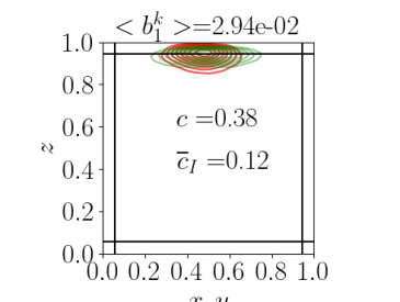 |
 |
 |
 |
| CBL | 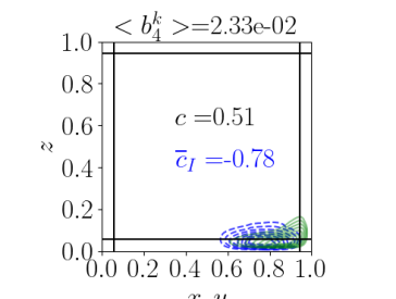 |
 |
 |
|
| VEZ | 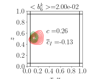 |
 |
||
| VBL | 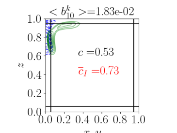 |
 |
 |
|
| HEZ | 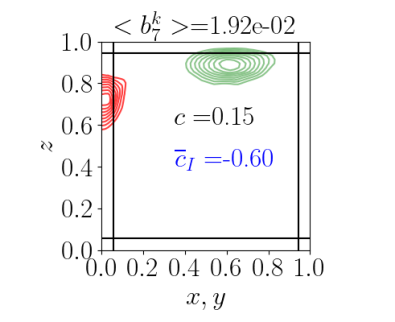 |
 |
 |
 |
| HBL |  |
 |
 |
||
| CBL | 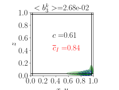 |
 |
 |
 |
|
| VEZ | 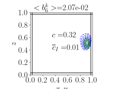 |
 |
 |
 |
|
| VBL | 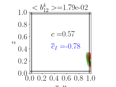 |
 |
|||
| HEZ | 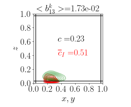 |
 |
| HBL | 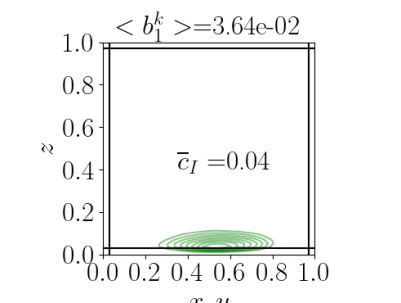 |
|||||
| HEZ | 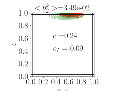 |
 |
 |
|||
| HEZ | 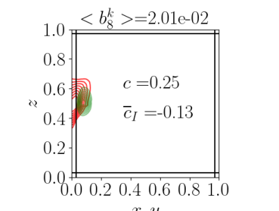 |
 |
 |
|||
| CBL | 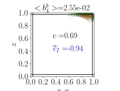 |
 |
 |
 |
||
| VBL | 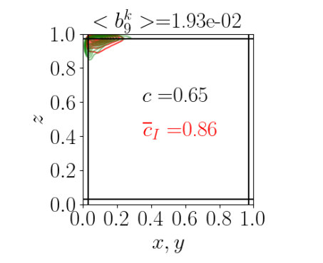 |
 |
 |
VEZ |

|