Hardware Honeypot: Setting Sequential Reverse Engineering on a Wrong Track

Abstract

Reverse engineering of finite state machines is a serious threat when protecting designs against reverse engineering attacks. While most recent protection techniques rely on the security of a secret key, this work presents a new approach: hardware state machine honeypots. These honeypots lead the reverse engineering tools to a wrong, but for the tools highly attractive state machine, while the original state machine is made less attractive. The results show that state-of-the-art reverse engineering methods favor the highly attractive honeypot as state machine candidate or do no longer detect the correct, original state machine.

I Introduction

RE is a serious threat in the silicon supply chain, endangering reliability, confidentiality, and integrity of intellectual property. In particular, the FSM of the design is of special interest to an attacker, because it reveals what makes a design: the design’s functionality.

To prevent RE of FSM, FSM obfuscation methods which lock the functionality with secret keys, dynamically changing keys, or input pattern may be used [1, 2, 3, 4, 5, 6]. Obfuscation schemes without a potentially attackable locking key are an alternative, like methods based on camouflaging techniques [7, 8]. Camouflaging, however, often requires a foundry to be able to implement it into the design, like adding a thin isolating layer to gate contacts [7], or has to reveal its camouflaged information, like the timing behavior [8], to the foundry to be producible. This work, in contrast, presents a new technique which is not based on foundry-enabled camouflaging or on locking. It hinders state-of-the-art RE methods to successfully identify the entire set of correct FSM gates in a gate-level netlist by exploiting characteristics of RE methods. In addition and similar to [7], it leads the attacker to a wrong, designer-controlled FSM.

To extract an FSM in a gate-level netlist, several sequential RE methods were developed. They first identify the FF of the FSM, so-called SFF, and all other combinatorial gates belonging to the FSM. In a second step, they extract the state transition graph [9]. Many state-of-the art sequential RE methods do not fully investigate the extraction of multiple FSM [10]. There are methods which extract multiple FSM candidates, but do not further elaborate on how to choose the correct FSM out of multiple FSM candidates [11, 12]. Other methods extract only one FSM candidate [13, 14]. Thus, the existence of multiple FSM within a design complicates sequential RE. In addition, current SFF identification methods are heuristic approaches which use specific—often similar—features to identify SFF.

TABLE I: Overview of SFF features which are exploited by state-of-the-art SFF identification methods.

Method	High FP	Any FP	Grouping based on	Effect on	Dissimilarity	Influence/dependency	Other structural
			‘clock’ or ‘enable’ or ‘reset’	control signals		behavior or SCC	features
[9]	✓
[11]	✓		✓	✓		✓
[15, 16, 17]					✓
[18, 19]					✓	✓	✓
[13]		✓			✓
[12]		✓			✓	✓
[20]	✓		✓	✓		✓
[14]						✓	✓

We take advantage of these two properties and present a novel two-part FSM obfuscation methodology to prevent sequential RE, see Fig. 1.

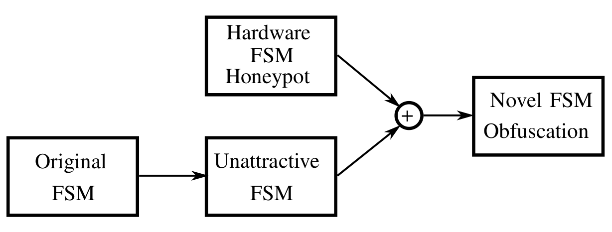
Figure 1: Novel two-part FSM obfuscation approach: hiding the original FSM by making it less attractive (unattractive FSM) and providing an attractive alternative in form of a hardware FSM honeypot

• We introduce hardware FSM-HP which satisfy features of the SFF identification methods. FSM-HP pretend to be the correct FSM of the design, which causes attackers to stop their effort to extract further FSM and thus prevents the extraction of the correct FSM. To ensure that state-of-the-art sequential RE methods identify the FSM-HP as a single FSM, or as best suitable candidate, we design the FSM-HP to be more attractive than the correct FSM.

• We obfuscate the original FSM, now called unattractive FSM, by eliminating features of certain SFF identification methods. As a result, unattractive FSM are resistant to these FSM identification methods. A similar approach was recently presented in the context of HT insertion [21]. The work inserts HT which have weaker features of HT detection techniques to circumvent them.

• We combine both techniques, FSM-HP and unattractive FSM, to enhance the effect of both.

FSM-HP can be implemented on RTL level or on gate level, allowing the designer to freely control design properties or design functionality. This allows them to increase the attractiveness of the FSM-HP and engage an attacker with controlled, false information. The results show that by using our novel FSM obfuscation methodology, state-of-the-art SFF identification methods favor the SFF of the FSM-HP or can no longer identify the correct SFF, leading to a wrong FSM extraction.

In the following, section II presents preliminaries and a systematic background overview, including an analysis of the exploitable FSM extraction features. Section III presents the novel obfuscation approach, in particular FSM-HP and unattractive FSM. The obfuscation and overhead results are analysed in section IV. Section V concludes the work.

II Systematic Background Analysis

To identify similar features which can be exploited to artificially modify the attractiveness of FSM, we first introduce preliminaries and then systematically summarize and compare the FSM extraction algorithms, in particular the SFF identification methods.

II-A Preliminaries

In the following, we introduce FSM and further define two of their structural characteristics, the path properties and connectivity.

II-A1 FSM

The state transition graph of an FSM consists of a set of states, inputs, and transitions, and a reset state [22]. Synthesis translates the FSM into a gate-level netlist. A set of FF, so-called SFF or the state register, hold the FSM state, while their combinatorial input cone, so-called next state logic, updates the FSM state for each clock cycle, implementing the state transitions.

II-A2 Path Properties

The work in [12] introduces three different strengths for paths between two FF: high, medium, and low. A high strength path contains only combinatorial gates, a medium strength path contains combinatorial gates and SFF, while a low strength path contains all types of gates and FF. We call a path from a FF to itself a FP. State FF usually have a FP, often with a high strength (high FP) [12].

II-A3 Strongly Connected Component

A SCC is a set of connected nodes in a graph with the following properties: 1) there is a path in the graph from every node to every other node in the set, 2) every node which satisfies property 1) is part of the set. In netlists, gates map to nodes and wires map to edges in the graph; a SCC thus is a set of strongly connected gates. The authors in [23] developed Tarjan’s algorithm, an efficient algorithm to identify SCC. In the following, we define two SCC of a netlist to be special SCC: the FSM SCC contains all or the majority of SFF of the original FSM, and the FSM-HP SCC contains all or the majority of SFF of the FSM-HP. However, due to SCC-property 2), both special SCC might also contain other FF in addition to the SFF of the original FSM or of the FSM-HP. All other multi-element SCC are defined as data SCC.

II-B FSM Extraction

During gate-level sequential RE, FSM extraction requires multiple steps: 1) identify all FF which contain the FSM state, i.e. SFF; 2) identify all further netlist elements which determine the FSM states, i.e. all gates in the region of the SFF; 3) extract the state transition graph by determining all possible next states for a current state and all possible input combinations, starting from the reset state [9, 24]. Steps 2) and 3) can be solved by netlist tracing or Boolean function evaluation. They are exact approaches for given SFF and reset state. Identifying the correct SFF, however, is a more challenging task, for which currently only heuristic approaches exist. Consequently, the success of retrieving a correct state transition graph can be measured by the success of identifying the correct SFF.

Table I provides an overview of state-of-the-art methods to identify SFF from a reverse engineered gate-level netlist, and an overview of their applied features: high FP; FP of any strength; dependency on the same clock, reset, or enable signal; influence on the design’s control signals; dissimilar gate-level structures of their input cones; type or level of influence or dependency between them, ranging from loosely connected to strongly connected, e.g. SCC; further structural features, like gate types in the input cone. The table shows what features each method uses for the identification and thus, shows methods with similar features or frequently applied features.

The methods [9, 11] identify SFF to be FF with a high FP [9] or FF with a high FP and an influence on control signals [11]. [11] additionally group FF based on enable signals and SCC to identify suitable registers.

The authors of RELIC [15] classify FF into state and non-state FF by determining the dissimilarity of their input cones. FF with less similar input cones are classified as SFF. With grouping, authors in [13] and [16] improved the performance of the approach. To improve the results, the work in [13] also checks a potential SFF for the existence of low, medium or high FP. The work in [12] introduces a structural post-processing based on connectivity and path strength, while the method in [17] replaces the structural similarity determination by a functional similarity determination. The netlist analysis toolset NetA [18, 19] includes some implementations of RELIC, one of these extends the original method by a PCA and structural features resulting in a Z-Score value for each FF signal. The higher the Z-Score value, the more likely it is that the FF represents a SFF. The authors of NetA suggest combining RELIC with SCC identification (RELIC-Tarjan). For the suggested combination, RELIC only identifies the most likely SFF, i.e. the signal with the highest Z-Score value. This FF is then used to identify the remaining SFF. With Tarjan’s algorithm, NetA determines all SCC within the FF of the netlist and then selects the SCC which contains the most likely SFF. Finally, it classifies all FF of the selected SCC as SFF.

The method in [20] combines different approaches of previous methods and adds new techniques. First, a topological analysis groups FF based on FF types and enable, clock and reset signals. Next, the algorithm splits these groups of FF based on existing SCC. Then, it removes FF if they do not have a high FP or do not have enough influence on each other. Finally, it removes SFF groups if one of its SFF does not have enough effect on control signals.

A recent method [14] uses GNN and structural features to identify state FF. The features include the number of gate types, of inputs, and of outputs, and graph metrics, like the betweeness centrality and the harmonic centrality. The method additionally adds a post-processing which removes all FF which are not part of an SCC.

II-C Exploitable FSM Extraction Features

By analyzing and comparing state-of-the-art SFF identification methods, we identify features which are frequently used, like the high FP, the dissimilarity, or the influence/dependency behavior. Thus, these features form good target features when designing attractive FSM-HP, see section III-A.

In addition, we identify two features which have a significant impact on the success of identification methods and can be avoided during FSM design: high FP and dissimilarity (highlighted in Table I). We show that these two features can be exploited to build unattractive FSM. We change FSM designs such that not all of their SFF possess all of these features without changing their original functionality, see section III-B. As a result, SFF identification methods which use these features will not correctly identify all SFF, and thus a correct RE of unattractive FSM will fail.

Also, adapting SFF identification approaches to better identify unattractive FSM is no promising solution. If identification methods would use less restrictive features, such that they also identify SFF of unattractive FSM, the false positive rate, i.e. the number of FF which are wrongly identified as SFF, will drastically increase.

III Methodology

In the following, the two parts of the new FSM obfuscation methodology are introduced: hardware FSM-HP and unattractive FSM.

III-A Hardware FSM Honeypot

The first part of the new FSM obfuscation methodology are hardware FSM-HP, which pretend to be the correct FSM. These FSM-HP must be more attractive for sequential RE methods than the original FSM, so that only the FSM-HP are identified as FSM. We assume that no further limitations exist for FSM-HP.

An FSM-HP will be added to the original design, e.g. as a separate module. To avoid an easy detection due to its isolated, unconnected appearance, we use original design inputs as inputs for the FSM-HP, in particular the original design’s reset and clock signal. The outputs of the FSM-HP should pretend to control the design behavior, e.g. by using techniques like dummy contacts [25] or never activated paths. Additionally, the more of the typical FSM features an FSM-HP fulfills—like the ones in Table I—the more attractive it becomes for state-of-the-art RE methods. Two highly relevant features are high FP and a high connectivity, which means that the SFF of the FSM-HP belong to the same SCC. Both features can be easily verified for a gate-level netlist representation of an FSM-HP design.

III-B Unattractive FSM

The second part of the new FSM obfuscation methodology are unattractive FSM, which help to make FSM-HP more attractive than the original FSM. An unattractive FSM has a specific design which exploits a feature of one or more specific SFF identification algorithms, see section II-C. By designing an FSM so that it specifically does not fulfill a certain SFF feature, which is a feature for a SFF identification algorithm, the algorithm and thus the FSM extraction fail. There exist different strategies how to achieve such an FSM design. Either the designer is aware of the requirements and designs the FSM accordingly, or an existing FSM is redesigned without changing the original functionality. If possible, the second strategy is preferred, as it can be done independent of the FSM design process. In the following, we introduce two redesign methods to build an unattractive FSM, based on the identified features in section II-C: dissimilarity and high FP.

III-B1 Dissimilarity Approach

The dissimilarity feature makes use of the fact that the input structure of SFF is usually less similar than the input structure of data FF, because due to data words, data bits are often processed in a similar way [15]. An unattractive FSM should have a low dissimilarity, and thus a high similarity score. One can calculate a similarity score for an FF by comparing its FF input structure with all other FF input structures of the design [15]. To increase the similarity score of SFF input structures, we replicate each state bit in the RTL description multiple times. As an example, assume an FSM with three state bits and the following six states $\{S_{1},\dots,S_{6}\}$:

$$S_{1}=000,S_{2}=001,S_{3}=010,S_{4}=011,S_{5}=100,S_{6}=101$$

After replicating each state bit twice (marked in blue), the six states have following labels:

$$S_{1}=0{\color[rgb]{0,0,1}00}0{\color[rgb]{0,0,1}00}0{\color[rgb]{0,0,1}00},S_{2}=0{\color[rgb]{0,0,1}00}0{\color[rgb]{0,0,1}00}1{\color[rgb]{0,0,1}11},S_{3}=0{\color[rgb]{0,0,1}00}1{\color[rgb]{0,0,1}11}0{\color[rgb]{0,0,1}00},$$

$$S_{4}=0{\color[rgb]{0,0,1}00}1{\color[rgb]{0,0,1}11}1{\color[rgb]{0,0,1}11},S_{5}=1{\color[rgb]{0,0,1}11}0{\color[rgb]{0,0,1}00}0{\color[rgb]{0,0,1}00},S_{6}=1{\color[rgb]{0,0,1}11}0{\color[rgb]{0,0,1}00}1{\color[rgb]{0,0,1}11}$$

The synthesis options are modified so that no re-encoding of the FSM and no merging of the FF occur and thus the replicated state bits are translated into individual FF. As a result, all FF representing the replicated bits of one state bit will have a highly similar input structure that increases the overall similarity score of these SFF and makes them more difficult to identify as SFF.

In the specific case of RELIC-Tarjan [18, 19], it may not be sufficient to solely increase the similarity of SFF, i.e. solely decrease the Z-Score values of SFF signals, because RELIC-Tarjan uses only the signal with the highest Z-Score value to identify the corresponding set of SFF (see section II-B). As a consequence, the identification will also succeed if any FF of the FSM SCC—even if it is not a SFF—has the highest Z-Score value.

To show an example, assume an FSM has two SFF signals, $F^{s}_{1}$ and $F^{s}_{2}$, which belong to the same FSM SCC, $scc$, and $scc$ additionally contains three other, non-SFF signals, $F_{1}$, $F_{2}$, and $F_{3}$:

$$scc:\left\{F^{s}_{1},F^{s}_{2},F_{1},F_{2},F_{3}\right\}$$

Assume that before applying the dissimilarity approach, RELIC-Tarjan determines the highest Z-Score value to be 622 and that it belongs to $F^{s}_{2}$:

$$scc:\left\{\begin{array}[]{cc}F^{s}_{1}:&\text{Z-Score}=512\\ \mathbf{F^{s}_{2}:}&\textbf{\text{Z-Score} = 622}\\ F_{1}:&\text{Z-Score}=84\\ F_{2}:&\text{Z-Score = 389}\\ F_{3}:&\text{Z-Score}=110\end{array}\right\}$$

Thus, all FF signals in $scc$ will be identified as SFF, including the correct SFF signals, $F^{s}_{1}$ and $F^{s}_{2}$. After applying the dissimilarity approach on all SFF, the Z-Score values of $F^{s}_{1}$ and $F^{s}_{2}$ are decreased. However, it might happen that now the highest Z-Score value is 389 which again belongs to one of the FF signals in $scc$, namely $F_{2}$:

$$scc:\left\{\begin{array}[]{cc}F^{s}_{1}:&\text{Z-Score}=178\\ F^{s}_{2}:&\text{Z-Score}=209\\ F_{1}:&\text{Z-Score}=84\\ \mathbf{F_{2}:}&\textbf{\text{Z-Score = 389}}\\ F_{3}:&\text{Z-Score}=110\end{array}\right\}$$

Consequently, again all FF signals in $scc$—including $F^{s}_{1}$ and $F^{s}_{2}$—are classified as SFF, what hinders a successful obfuscation.

To prevent this, one could replicate all signals from the FSM SCC; however, for most cases, replicating state and counter bits is sufficient, because they often have the highest Z-Score values. Counter bit replication appears to be more challenging than state bit replication, because counters usually have significantly more states than FSM, e.g. 256 states for an 8-bit counter. Furthermore, in contrast to states, counters are usually not assigned within a case structure, but by assignments which count up or down. We developed a technique which allows a counter bit replication without using a costly case structure for the counter state assignment. We add an extra counter wire to first increment or decrement the counter and then assign the replicated bits to the same value of the original counter bit. This method is valid as long as no counter over- or underflow occurs. As an example, assume a 3-bit counter register c, which counts up using the following source code in the original design:

c <= c + 1;

We replicate each counter bit twice, by adding a 9-bit temporary c_t and following code lines:

c_t = c + 1;
c[8:6] <= (c_t[8:6]==3’b001)?3’b111:c_t[8:6];
c[5:3] <= (c_t[5:3]==3’b001)?3’b111:c_t[5:3];
c[2:0] <= (c_t[2:0]==3’b001)?3’b111:c_t[2:0];

With this method, the similarity score of the FF belonging to the counter will increase, hindering the identification of the correct FSM SCC.

III-B2 FP Approach

The high FP feature makes use of the fact that SFF usually have a high FP. This feature was one of the first features used for SFF identification [9, 11] and is still used in recent approaches [20].

Recently, an FSM obfuscation method was published which requires SFF without high FP to apply a camouflaging technique [8]. Thus, the work developed two methods to avoid a high FP for a SFF by redesigning an FSM: $R_{A}$ which is applied on one-hot-encoded FSM and on gate-level netlists, and $R_{B}$ which is applied on binary-encoded FSM and on RTL code, see Fig. 2.

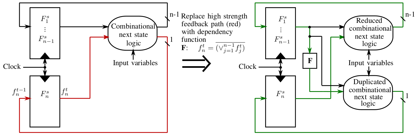
(a) $R_{A}$: Replace the output signal of the SFF $F^{s}_{n}$ at time $t$, $f_{n}^{t}$, which forms the high FP (highlighted in red), with the Boolean function F, which represents the definition of one-hot encoding. This results in a removed high FP for $F^{s}_{n}$ (highlighted in green). [8]

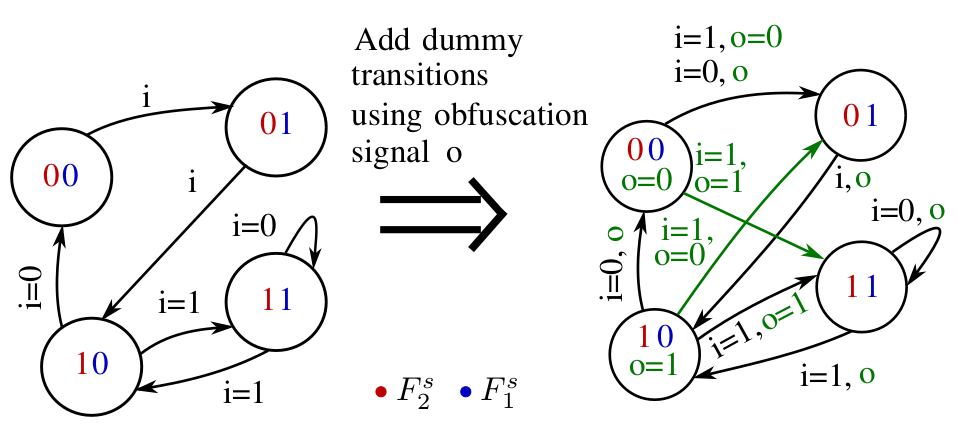
(b) $R_{B}$: Add artificial dummy transitions to the example FSM which are controlled by the obfuscation signal ‘o’, such that the red state bit can be determined without using its previous value. This results in a removed high FP for $F^{s}_{2}$. [8]

Figure 2: Two techniques for the FP approach to remove a high FP: $R_{A}$ and $R_{B}$

$R_{A}$ partially disconnects a SFF from posterior logic, in such a way that the high FP is removed, see the example in Fig. 2(a). Where disconnected, the signal is replaced by a Boolean function F that outputs one if all other SFF values equal zero—the definition of one-hot encoding. $R_{B}$ adds extra, dummy transitions to the RTL description of the FSM and controls them by an obfuscation signal, see the example in Fig. 2(b). The dummy transitions are designed such that one of the FSM bits can always be determined without considering its own value, i.e. using only the other FSM bit values and inputs. As a result, both methods ensure that at least one of the SFF of an FSM does not influence itself within one clock cycle. Consequently, this SFF is free of high FP while the original FSM functionality does not change.

We adopt these techniques by using the resulting, redesigned FSM as unattractive FSM. State FF identification methods which use high FP as feature will no longer identify this SFF with medium or low FP. This results in an unsuccessful SFF identification and thus, in an unsuccessful FSM extraction.

III-C Design Options and Complexities

The design options and complexities to generate unattractive FSM are defined by the applied redesign method. While the dissimilarity approach is implemented by hand, the redesign method of the FP approach can be partly automated and had been shown to have short runtimes, see the results in [8].

In contrast to unattractive FSM, there are various options how to design an FSM-HP. They can be build as RTL code or as gate-level netlists, by hand or automatically by a generator, with identical or changed synthesis options. Each design option has different advantages and disadvantages. Designing on RTL level or by hand allows for an FSM-HP with a user-defined functionality. This enables FSM-HP which lead the attacker to targeted wrong conclusions about the design. Designing on gate-level netlist enables a better control over the final netlist structure, because the synthesis will not determine the gate representation itself. Better control can ease the achievement of attractive gate-based features, like dissimilarity. If the FSM-HP is designed automatically by a generator, one can create a high number of FSM-HP variations in a short time. By providing different parameters or adding specific conditions to the generator, the designed FSM-HP can be forced to satisfy predefined features, like number of state bits or high FP. Separate synthesis processes for the original FSM and the FSM-HP are also possible. This allows the designer to maintain all design specific synthesis settings for the original design, while choosing suitable settings for the FSM-HP to achieve maximum attractiveness.

The complexity of generating an FSM-HP is independent of the remaining design. Thus, the complexity does not change whether the FSM-HP is generated for a toy example or for an industrial design. When using automatic FSM-HP generators, instead of generating it by hand, the runtime to build an FSM-HP can be negligibly small.

IV Results

We demonstrate the different obfuscation approaches using nine open-source designs, including designs from OpenCores (aes_core [26], altor32_lite [27], fpSqrt [28], gcm_aes [29], a uart based on [30]), cryptography designs (sha1_core [31], siphash [32]), and a submodule as well as a complete core of a RISC-V processor (mem_interface [33], picorv32 [34]). For synthesis, the open-source tools qflow [35] and yosys [36] are applied without adding specific timing constraints. Table II provides additional information on the designs and their synthesized netlists: the number of FF, of multi-element SCC, of FSM, of SFF per FSM, and the encoding of the FSM states after synthesis. The synthesis setup optimizes all identified FSM, resulting in a one-hot encoding for most of the designs. Three designs, $\alpha)$, $\beta)$, and $\iota)$ consist of only a single source code module, while all others are composed of a minimum of two modules. The use of the 32-bit RISC-V core demonstrates the adaption for realistic designs.

We evaluate the obfuscation results using two SFF identification approaches: RELIC-Tarjan [19] and the topological analysis [20], see section II-B. The SFF identification is considered to be successful if 100% sensitivity is achieved, i.e. if all SFF are part of the identified set of SFF, regardless of how many non-SFF are wrongly identified as SFF. For the obfuscated netlists, we differ between the successful identification of SFF of the unattractive FSM and the successful identification of SFF of the FSM-HP. This allows us to evaluate the obfuscation approach.

TABLE II: Single and multi module benchmarks and their number of FF, multi-element SCC, FSM, SFF, and the type of encoding when synthesizing with default optimization settings

	Design	#FF	#SCC	#FSM	#SFF	encoding
					(per FSM)
$\alpha)$	uart	64	1	2	3,2	binary
$\beta)$	mem_int.	75	1	1	7	one-hot
$\gamma)$	siphash	794	2	1	8	one-hot
$\delta)$	sha1_core	850	3	1	3	one-hot
$\epsilon)$	aes_core	901	2	1	16	one-hot
$\zeta)$	altor32_l	1249	2	1	6	one-hot
$\eta)$	fpSqrt	1331	2	1	3	one-hot
$\theta)$	gcm_aes	1697	5	1	10	one-hot
$\iota)$	picorv32	1598	1	2	4,7	one-hot

IV-A RELIC-Tarjan

This section shows the successful obfuscation, using the dissimilarity approach combined with an FSM-HP, against similarity-based SFF identification. For each design, we synthesize the original and the obfuscated version. As explained in section III-B1, no FSM re-encoding is used to synthesize the obfuscated netlists. For comparability, we also deactivate the re-encoding when synthesizing the original netlists. As a result, some FSM of Table II remain binary-encoded instead of being optimized to one-hot encoding. We then evaluate the obfuscation by applying the RELIC-Tarjan approach on both netlists. We use designs with at least two multi-element SCC, i.e. designs $\gamma)-\theta)$, see Table II. The RELIC-Tarjan approach uses the tools relic and tjscc from the NetA toolset [19]. The tool relic extends the similarity measurement with a PCA and is used with its default settings and the option buf.

For the dissimilarity approach, we replicate state bits, and if necessary other signals of the FSM SCC, three, five, or 31 times, dependent on the achieved Z-Score reduction. The example in Fig. 3 shows the FSM of the design fpSqrt before and after the state bit replication. To design an FSM-HP, we copy the original FSM and modify some transitions or outputs of the copy. For some designs this process had to be repeated to receive an FSM-HP SCC element with a Z-Score value higher than those of the FSM SCC. We recognized an increased challenge to find such a suitable FSM-HP if the original FSM either has few state bits ($\leq 2$) or has a strong cyclic behavior. We assume that the SFF of such FSM have features beside the similarity score which are well identifiable by the tool relic. Note that it is realistic to assume that a designer is able to evaluate their FSM-HP for such features, e.g. regarding Z-Score values: a designer also has access to RE tools and can thus apply them.

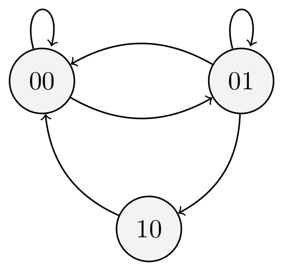
(a) Original FSM

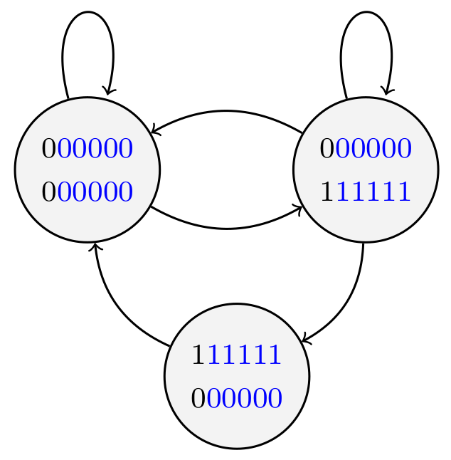
(b) Unattractive FSM

Figure 3: FSM encoding of the design fpSqrt before and after replicating its state bits five times

Fig. 4 plots the maximum Z-Score value of the FF in any data SCC and the maximum Z-Score of the FF in the FSM SCC using the original netlists ($\mathcal{A}$), compared against the maximum Z-Score value of the FF in any data SCC, the maximum Z-Score value of the FF in the FSM SCC, and the maximum Z-Score of the FF in the FSM-HP SCC using the obfuscated netlists ($\mathcal{Z}$). The figure shows that the obfuscation succeeds for all designs, as an FSM-HP could always be designed such that at least one FF in its SCC has a higher Z-Score value than any FF of the FSM SCC (compare the green circles and the black crosses for the obfuscated netlists $\mathcal{Z}$). Due to the dissimilarity approach, for all designs, the maximum Z-Score value of the FF in an FSM SCC decreased for the obfuscated design. We highlight this change with blue arrows. For the majority of designs, we achieve the ideal case: the maximum Z-Score value for the FF of the original FSM SCC is below the maximum Z-Scores for the FF of data SCC and the FSM-HP SCC. Summarizing, the RELIC-Tarjan procedure will identify the FSM-HP as best FSM candidate, allowing a successful FSM obfuscation.

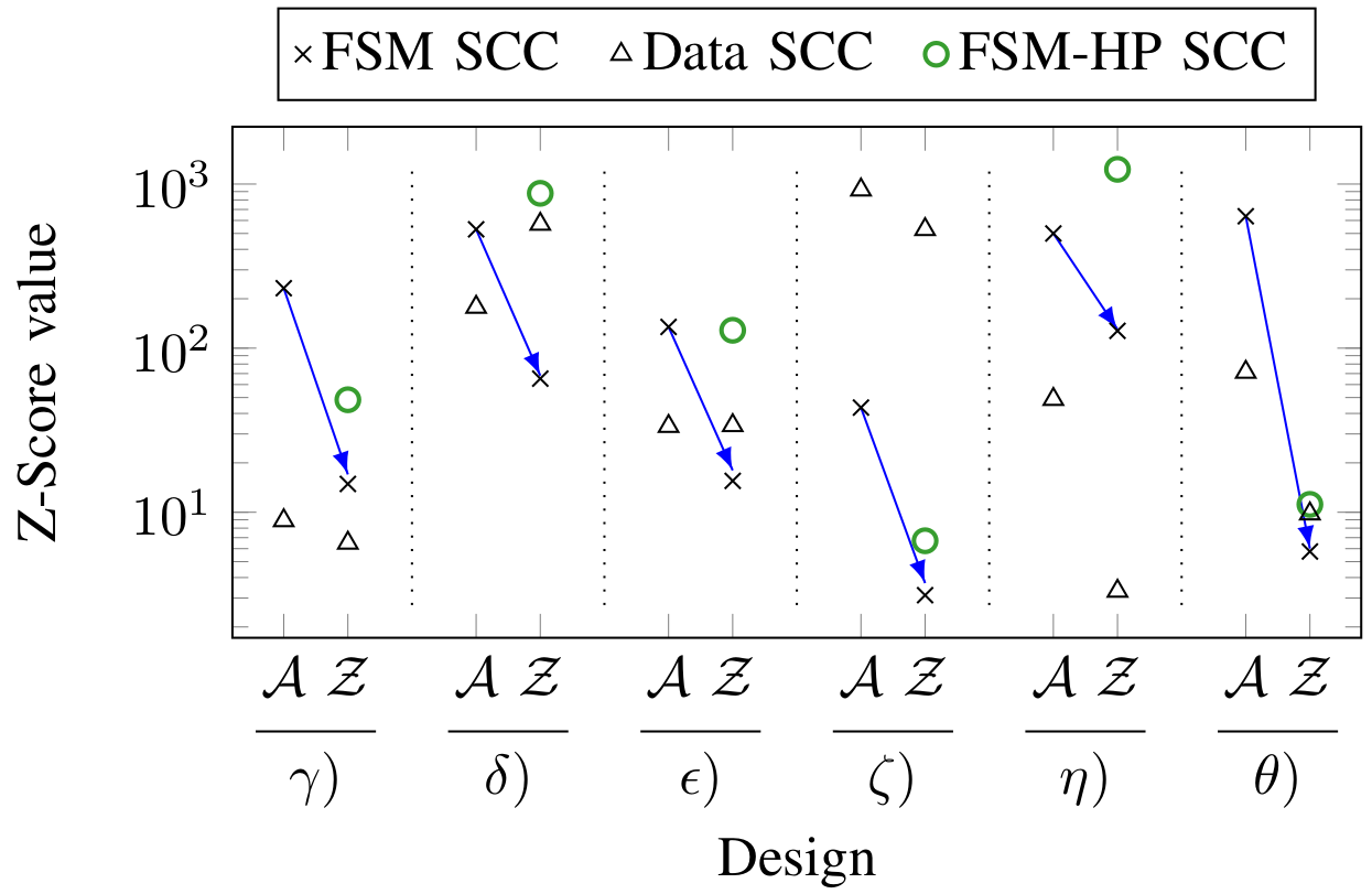
Figure 4: Maximum Z-Score value of the FF in any data SCC and of the FF in the FSM SCC before ($\mathcal{A}$) and after ($\mathcal{Z}$) obfuscation, and maximum Z-Score value of the FF in the FSM-HP SCC

TABLE III: Identifying SFF with Topological Analysis with and without obfuscation (✓: all correct SFF identified, ($x$/$y$): $x$ out of $y$ SFF correctly identified resulting in a successful obfuscation)

Design	without	with FP approach
	obfuscation	and FSM-HP
	orig. FSM	orig. FSM	FSM-HP
$\alpha)$	✓	(1/2), (2/3)	✓
$\beta)$	✓	(0/7)	✓
$\gamma)$	✓	(7/8)	✓
$\iota)$ 1	✓	(3/4)	✓

• FSM of the memory interface

IV-B Topological Analysis

The following section shows the successful obfuscation using the FP approach combined with an FSM-HP against topological-analysis-based SFF identification. We use four designs of Table II for which the topological analysis is able to extract an FSM candidate with all SFF of the original FSM, see the second column of Table III. As discussed in section II-B, the last step of the topological analysis is the determination of the control behavior of FF. We slightly adapt this step in our implementation of the topological analysis, because without this adjustment, our obfuscation worked too easily: Instead of removing the FSM candidate as a whole if one FF does not show any control behavior [20], our implementation only removes the FF itself. Due to performance limitations of our topological analysis implementation, for the picorv32, the output control behavior calculation could not be finished for each SFF candidate. Thus, Table III shows the results for picorv32 without performing the last step, the output control behavior calculation. However, the actual obfuscation results are assumed to improve further, because this last step would remove additional FF of FSM candidates.

For the FP approach, we apply one of the two FSM redesign methods on an arbitrary state bit or SFF of the original FSM: $R_{A}$ for the one-hot-encoded designs, and $R_{B}$ for the binary-encoded design. When applying the FSM-HP, in contrast to the demonstration in section IV-A, the same FSM-HP is added to all designs, only the inputs are changed to match the inputs of the original design.

Applying topological analysis on these obfuscated designs leads to no or only partly identified SFF of the original FSM, and instead of that, to successfully identified SFF of the FSM-HP, see columns three and four of Table III. Consequently, the output of the topological analysis on these obfuscated designs can lead to one of the following two results:

• No FSM candidate contains any SFF of the original design. As a result, data FF or the FSM-HP FF will be used to extract an incorrect FSM.

• An FSM candidate contains parts of the original SFF. As a result, the subset of SFF or data FF or FSM-HP FF will be used to extract an incorrect FSM.

Both cases successfully prevent the correct extraction of the original FSM.

IV-C Overhead

This section discusses the cell area and delay overhead of the developed two-part FSM obfuscation, i.e. of adding an FSM-HP and of translating the original FSM to an unattractive FSM. We measure the cell area and the timing with proprietary EDA tools, assuming a frequency of $20\text{\,}\mathrm{MHz}$.

In average, the obfuscated designs in section IV-A have 51%, the obfuscated designs in section IV-B 8% more cell area than the original designs in Table II, see the results in Table IV. Thus, the generated overheads are larger and smaller than the measured overheads of a recently published FSM obfuscation method in [5] which reported 24% area overhead on average, or both smaller than another recently published FSM obfuscation method in [6] which reported 288% area overhead on average. Compared to the topological results, the RELIC-Tarjan results have a significantly larger overhead. We assume that this is preliminary due to the dissimilarity approach, in particular due to the logic which is replicated when replicating bits, like state or counter bits, in the RTL code. However, as the obfuscation targets the FSM and an FSM is usually the smallest part of a design, our measured average overhead results should decrease for larger, industrial designs. Overall, the obfuscation overhead preliminary depends on the number of replicated bits, on the number of FSM in a design which must be obfuscated, and on the size of the FSM —which varies significantly less than design sizes. For designs with multiple FSM, the designer can decide to only obfuscate security critical or proprietary FSM to decrease the area overhead. In addition, when obfuscating multiple FSM, the designer can choose to add only a single FSM-HP for all unattractive FSM, instead of adding an FSM-HP for each unattractive FSM. This also decreases the area overhead.

In contrast to the area overhead and in contrast to the recent obfuscation methods in [5] and [6], the timing, i.e. the circuit slack, is not effected negatively by the novel two-part FSM obfuscation method. For our benchmarks, in average, the slack time is even decreased, resulting in 0.7% less slack time for the obfuscated designs in section IV-A and 2% less slack time for the obfuscated designs in section IV-B, see the results in Table IV.

TABLE IV: Cell area and delay overhead results for the novel two-part FSM obfuscation

	Dissimilarity approach		FP approach
Design	Area (%)	Delay (%)	Area (%)	Delay (%)
$\alpha)$	-	-	27.72	-0.80
$\beta)$	-	-	8.03	-1.09
$\gamma)$	77.71	0.08	-0.27	-0.68
$\delta)$	100.07	-1.72	-	-
$\epsilon)$	3.71	0.08	-	-
$\zeta)$	5.72	-0.41	-	-
$\eta)$	99.00	-2.09	-	-
$\theta)$	19.34	0	-	-
$\iota)$	-	-	-4.35	-5.42
Average	50.93	-0.68	7.78	-2.00

V Conclusion

The work presents a two-part state machine obfuscation approach to prevent sequential RE: hardware FSM honeypots and unattractive FSM. Using one similarity-based and one topological-analysis-based SFF identification method, we demonstrate that state-of-the-art RE tools favor the more attractive FSM-HP or cannot correctly identify the unattractive original FSM. This leads to a successful obfuscation of the original FSM, and allows control over what will be identified by the attacker.

The novel obfuscation approach is extendable by investigating other RE tool assumptions and features which can be exploited for unattractive FSM. Also, the attack complexity for a reverse engineer can be increased if more than one honeypot is added to a design. In addition, if new identification mechanisms with new features are developed, the honeypot generation can be adapted accordingly and new techniques for translating the original FSM into an unattractive FSM can be investigated. Thus, the obfuscation approach has the potential to be secure also for novel identification techniques.

References

- [1] Rajat Subhra Chakraborty and Swarup Bhunia “HARPOON: An Obfuscation-Based SoC Design Methodology for Hardware Protection” In IEEE Transactions on Computer-Aided Design of Integrated Circuits and Systems 28.10, 2009, pp. 1493–1502
- [2] Kyle Juretus and Ioannis Savidis “Time Domain Sequential Locking for Increased Security” In 2018 IEEE International Symposium on Circuits and Systems (ISCAS), 2018, pp. 1–5 IEEE
- [3] Leon Li and Alex Orailoglu “JANUS-HD: Exploiting FSM Sequentiality and Synthesis Flexibility in Logic Obfuscation to Thwart SAT Attack While Offering Strong Corruption” In Proceedings of the 2022 Conference & Exhibition on Design, Automation & Test in Europe, DATE ’22, 2022, pp. 1323–1328
- [4] Rajit Karmakar, Santanu Chatopadhyay and Rohit Kapur “Encrypt Flip-Flop: A Novel Logic Encryption Technique For Sequential Circuits” In arXiv preprint arXiv:1801.04961, 2018
- [5] Md Moshiur Rahman and Swarup Bhunia “Practical Implementation of Robust State Space Obfuscation for Hardware IP Protection” In TechRxiv preprint 10.36227/techrxiv.21405075.v1, 2022
- [6] Leon Li and Alex Orailoglu “Thwarting Reverse Engineering Attacks through Keyless Logic Obfuscation” https://www.researchgate.net/publication/369090967_Thwarting_Reverse_Engineering_Attacks_through_Keyless_Logic_Obfuscation, 2023
- [7] Max Hoffmann and Christof Paar “Doppelganger Obfuscation — Exploring the Defensive and Offensive Aspects of Hardware Camouflaging” In IACR Transactions on Cryptographic Hardware and Embedded Systems 2021.1, 2020, pp. 82–108
- [8] Michaela Brunner, Tarik Ibrahimpasic, Bing Li, Grace Li Zhang, Ulf Schlichtmann and Georg Sigl “Timing Camouflage Enabled State Machine Obfuscation” In IEEE Physical Assurance and Inspection of Electronics (PAINE), 2022, pp. 1–7
- [9] Kenneth S McElvain “Methods and apparatuses for automatic extraction of finite state machines” US Patent No. US 6,182,268 B1, Filed Jan. 5th., 1998, Issued Jan. 30th., 2001 Google Patents, 2001
- [10] Rasheed Kibria, Nusrat Farzana, Farimah Farahmandi and Mark Tehranipoor “FSMx: Finite State Machine Extraction from Flattened Netlist With Application to Security” In 2022 IEEE 40th VLSI Test Symposium (VTS), 2022, pp. 1–7
- [11] Yiqiong Shi, Chan Wai Ting, Bah-Hwee Gwee and Ye Ren “A highly efficient method for extracting FSMs from flattened gate-level netlist” In Circuits and Systems (ISCAS), Proceedings of 2010 IEEE International Symposium on, 2010, pp. 2610–2613
- [12] Michaela Brunner, Alexander Hepp, Johanna Baehr and Georg Sigl “Toward a Human-Readable State Machine Extraction” In ACM Trans. Des. Autom. Electron. Syst. 27.6, 2022
- [13] Michaela Brunner, Johanna Baehr and Georg Sigl “Improving on State Register Identification in Sequential Hardware Reverse Engineering” In 2019 IEEE International Symposium on Hardware Oriented Security and Trust (HOST), 2019, pp. 151–160
- [14] Subhajit Dutta Chowdhury, Kaixin Yang and Pierluigi Nuzzo “ReIGNN: State Register Identification Using Graph Neural Networks for Circuit Reverse Engineering” In IEEE/ACM International Conference On Computer Aided Design (ICCAD), 2021, pp. 1–9
- [15] Travis Meade, Yier Jin, Mark Tehranipoor and Shaojie Zhang “Gate-level netlist reverse engineering for hardware security: Control logic register identification” In 2016 IEEE International Symposium on Circuits and Systems (ISCAS), 2016, pp. 1334–1337
- [16] Travis Meade, Kaveh Shamsi, Thao Le, Jia Di, Shaojie Zhang and Yier Jin “The Old Frontier of Reverse Engineering: Netlist Partitioning” In Journal of Hardware and Systems Security 2.3, 2018, pp. 201–213
- [17] James Geist, Travis Meade, Shaojie Zhang and Yier Jin “RELIC-FUN: Logic Identification through Functional Signal Comparisons” In 2020 57th ACM/IEEE Design Automation Conference (DAC), 2020, pp. 1–6
- [18] Travis Meade, Jason Portillo, Shaojie Zhang and Yier Jin “NETA: when IP fails, secrets leak” In Proceedings of the 24th Asia and South Pacific Design Automation Conference, 2019, pp. 90–95 ACM
- [19] Travis Meade, Shaojie Zhang and Yier Jin “NetA”, Available at https://github.com/jinyier/NetA, 2019
- [20] Marc Fyrbiak et al. “On the Difficulty of FSM-based Hardware Obfuscation” In IACR Transactions on Cryptographic Hardware and Embedded Systems 2018.3, 2018, pp. 293–330
- [21] Chi-Wei Chen, Pei-Yu Lo, Wei-Ting Hsu, Chih-Wei Chen, Chin-Wei Tien and Sy-Yen Kuo “A Hardware Trojan Insertion Framework against Gate-Level Netlist Structural Feature-based and SCOAP-based Detection” In 2022 IEEE 65th International Midwest Symposium on Circuits and Systems (MWSCAS), 2022, pp. 1–5
- [22] Edward F. Moore “Gedanken-experiments on sequential machines” In Automata studies 34, 1956, pp. 129–153
- [23] Robert Tarjan “Depth-first search and linear graph algorithms” In 12th Annual Symposium on Switching and Automata Theory (swat 1971), 1971, pp. 114–121
- [24] Travis Meade, Shaojie Zhang and Yier Jin “Netlist reverse engineering for high-level functionality reconstruction” In 2016 21st Asia and South Pacific Design Automation Conference (ASP-DAC), 2016, pp. 655–660
- [25] Lap-Wai Chow, James P. Baukus and William M. Clark “Integrated circuits protected against reverse engineering and method for fabricating the same using an apparent metal contact line terminating on field oxide” US Patent No. US 7,294,935 B2, Filed Jan. 24th., 2001, Issued Nov. 13th., 2007 Google Patents, 2007
- [26] OpenCores “AES128”, Available at https://opencores.org/projects/apbtoaes128, 2016
- [27] OpenCores “AltOr32 - Alternative Lightweight OpenRisc CPU”, Available at https://opencores.org/projects/altor32, 2015
- [28] OpenCores “FT816Float - Floating point accelerator”, Available at https://opencores.org/projects/ft816float, 2018
- [29] OpenCores “Galois Counter Mode Advanced Encryption Standard GCM-AES”, Available at https://opencores.org/projects/gcm-aes, 2010
- [30] OpenCores “Documented Verilog UART”, Available at https://opencores.org/projects/osdvu, 2016
- [31] Joachim Strömbergson “secworks sha1”, Available at https://github.com/secworks/sha1/tree/master/src/rtl, 2018
- [32] Joachim Strömbergson “secworks siphash”, Available at https://github.com/secworks/siphash/tree/master/src/rtl, 2016
- [33] OnchipUIS “mriscvcore”, Available at https://github.com/onchipuis/mriscvcore, 2017
- [34] YosysHQ “picorv32”, Available at https://github.com/YosysHQ/picorv32, 2022
- [35] Opencircuitdesign “qflow”, 2019 URL: http://opencircuitdesign.com/qflow/
- [36] Clifford Wolf “Yosys Open SYnthesis Suite”, 2018 URL: https://yosyshq.net/yosys/