The ELM Survey South. II.
Two dozen new low mass white dwarf binaries.

Abstract

We present the results from our ongoing spectroscopic survey targeting low mass white dwarf binaries, focusing on the southern sky. We used a Gaia DR2 and eDR3 based selection and identified 28 new binaries, including 19 new extremely low mass white dwarfs, one short period, likely eclipsing, DABZ, and two potential LISA binaries. We present orbital and atmospheric parameters for each new binary based on our spectroscopic follow-up.

Four of our new binaries show periodic photometric variability in the TESS 2-minute cadence data, including one new eclipsing double-lined spectroscopic binary. Three others show periodic photometric variability in ZTF, including one new eclipsing binary. We provide estimates for the inclinations and scaled component radii for these ZTF variables, based on light curve modeling to our high-speed photometric follow-up observations.

Our observations have increased the sample of ELM Survey binaries identified in the southern sky to 41, an increase of 64%. Future time domain surveys, such as BlackGEM and the Vera C. Rubin Observatory Legacy Survey of Space and Time, will efficiently identify the photometric variables in the southern sky and significantly increase the population of southern sky low mass white dwarf binaries, leading to a more complete all-sky population of these systems.

,

1 Introduction

Extremely Low Mass (ELM; $M\lesssim 0.3~{}{\rm M_{\odot}}$) white dwarfs are a relatively rare class of He-core white dwarfs which form after early severe mass loss. Because the main sequence lifetime of low mass stars can exceed a Hubble time, the ELM white dwarfs observed today are not expected to have formed through single star evolution. With an exception for the extreme mass loss of high-metallicity stars (see Kilic et al., 2007), ELM white dwarfs are expected to form through binary evolution, including one or more episodes of common envelope evolution (Li et al., 2019). The result of this binary evolution is a population of evolved compact binaries containing low mass He-core white dwarfs with evolved companions.

These low mass white dwarf binaries are important for studying both binary evolution and formation rates of various exotic systems. Shen (2015) and Brown et al. (2016b) show that most white dwarf binaries may merge and form other exotic systems such as extreme Helium stars (Zhang et al., 2014), accreting AM CVn binaries (Kilic et al., 2016), or massive single white dwarfs (Kilic et al., 2023). Binaries with well-constrained physical parameters have also been used to place constraints on the efficiency of common envelope ejection (see Scherbak & Fuller, 2023).

The ELM Survey (Brown et al., 2010; Kilic et al., 2011; Brown et al., 2012; Kilic et al., 2012; Brown et al., 2013; Gianninas et al., 2015; Brown et al., 2016a, 2020, 2022) is a spectroscopic survey targeting these low-mass white dwarf binaries based on photometry from sky surveys, such as SDSS (Abazajian et al., 2003) and PanSTARRs (Chambers et al., 2016). Kosakowski et al. (2020) expanded the ELM Survey into the southern sky using photometry from SkyMapper (Onken et al., 2019) and VST ATLAS (Shanks et al., 2015), and found that a Gaia based selection is efficient for identifying ELM white dwarf binaries. In total, previous ELM Survey studies have constrained the orbits and atmospheric parameters of 120 unique low mass white dwarf binaries (Brown et al., 2020; Kosakowski et al., 2020; Brown et al., 2022). Similar studies have created catalogs of ELM white dwarf candidates using Gaia DR2 astrometry (see Pelisoli & Vos, 2019) and single-epoch spectroscopy from LAMOST DR8 (see Wang et al., 2022), many of which still require follow-up observations to confirm their nature.

In this work, we continue the ELM Survey South with our search for low mass white dwarf binaries in the southern sky using a Gaia DR2 and eDR3. While we focused on objects in the southern sky, our Gaia based selection included many Northern sky objects, which we include in this work.

2 Target Selection

Our target selection made use of parallax and color measurements from Gaia DR2 and eDR3, based on previous ELM Survey discoveries. Figure 1 displays the locations of our observed objects on the Gaia DR3 color-magnitude diagram. The 28 new binaries from this work are plotted with blue symbols while previous ELM Survey binaries are plotted as black symbols. Green points represent other objects observed as part of this work with parallax_over_error¿3, parallax¿0.5, and no cuts to ruwe, for which we have obtained at least one optical spectrum. We draw a box around the region surrounding the main concentration of ELM Survey ELM white dwarf binaries, defined by

$$-0.24< (BP-RP)<0.34,$$

$$M_{\rm G}>4.31 (BP-RP)+5.53,$$

$$M_{\rm G}<4.31 (BP-RP)+10.53.$$

Within this box, we have observed 217 objects, including the 28 new LMWD binaries presented in this work. Among our observed objects, we identify 27 additional ELM white dwarf candidates based on model atmosphere fits to our follow-up spectroscopy, including 17 which fall within the parameter space of the “clean” sample of ELM white dwarfs of Brown et al. (2020). Our ongoing follow-up finds that at least half of these spectroscopic candidates show significant radial velocity variability, but have unconstrained orbital parameters. These additional binaries will be presented in a future publication. Most of our observed sample contains single white dwarfs with $\log{g}\approx 7.5$.

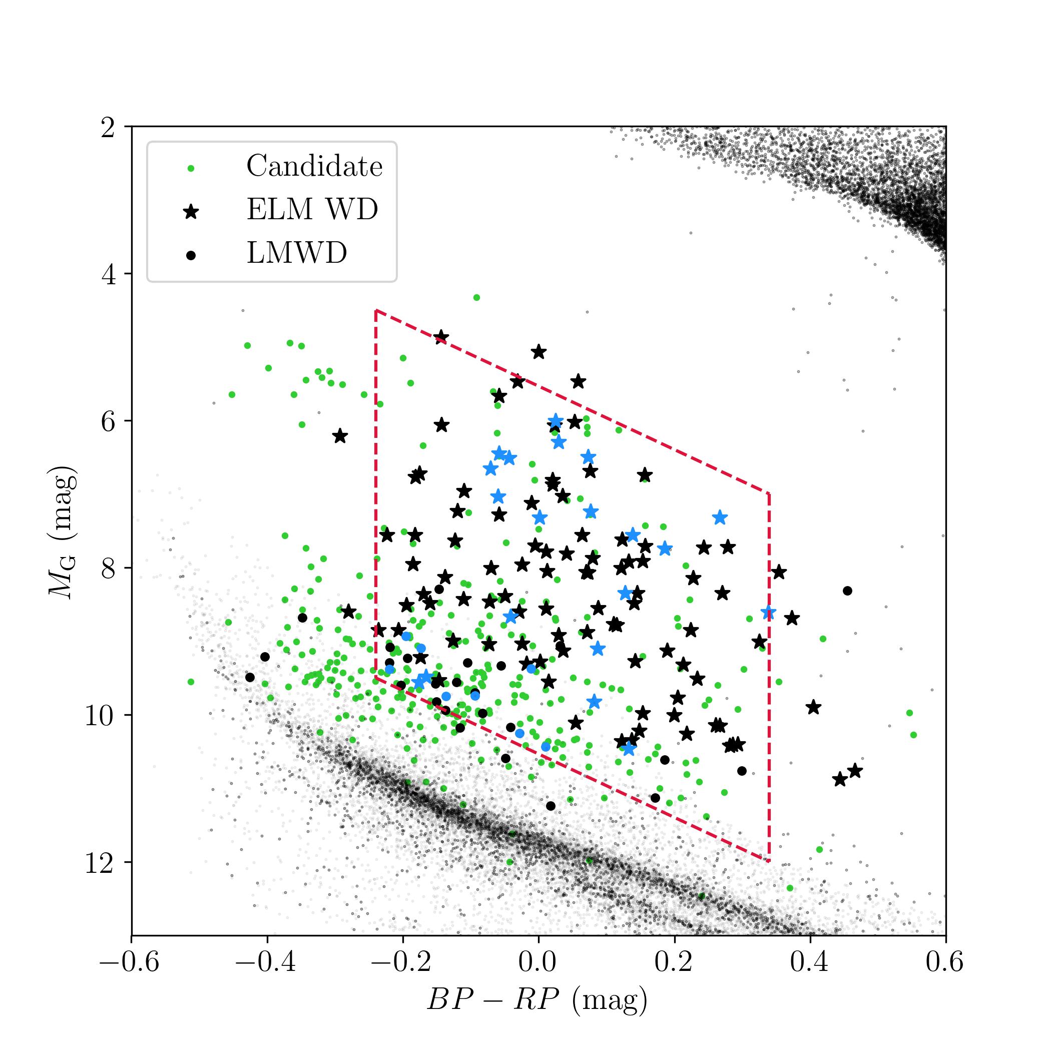
Figure 1: Gaia color-magnitude diagram showing the target selection box described in the text. The 28 new binaries identified in this work are represented with blue symbols, while the previous ELM Survey binaries are represented as black symbols. Stars represent ELM white dwarfs ($M\lesssim 0.3~{}{\rm M_{\odot}}$). Filled-circles represent low mass white dwarfs. Green circles represent our observed candidates selected through our Gaia DR2 and eDR3 selection.

3 Observations

We used a similar observing strategy as in previous ELM Survey publications: We obtained one optical spectrum for each of our candidates to confirm their nature and perform spectroscopic fitting with model atmospheres. For objects consistent with ELM white dwarfs ($5.0\lesssim\log{g}\lesssim 7.2$), we obtained multiple additional spectra to check for radial velocity variability and constrain orbital periods. Candidates which do not show significant radial velocity variability, or which show atmospheric parameters inconsistent with ELM white dwarfs, are excluded from extensive follow-up.

Our observing strategy favors identifying short period binaries ($P\lesssim 6~{}{\rm h}$) with large velocity semi-amplitudes, which form through common envelope interaction. Binaries with longer orbital periods and lower velocity semi-amplitudes, which likely form through stable Roche Lobe overflow, are less likely to be detected and constrained through our observing strategy, while those that are identified require more resources to constrain through radial velocity follow-up.

In this section we briefly describe the resources used for our follow-up observations, including the telescopes, instruments, and configurations.

3.1 Southern Astrophysical Research Telescope (SOAR)

We used the SOAR 4.1-meter telescope with the Goodman spectrograph (Clemens et al., 2004) configured with the $930~{}{\rm lines}~{}{\rm mm^{-1}}$ grating and $1.01\arcsec$ slit, resulting in a spectral resolution $\approx 2.6~{}{\rm\AA}$ over the wavelength range $3550-5300~{}{\rm\AA}$. These data were taken as part of the NOAO programs 2019B-0004, 2020B-0013, and 2021A-0007, and NOIRLab 2022A-161017.

3.2 Gemini South

We used the Gemini South 8.1-meter telescope, located on Cerro Pachón in Chilé, with the GMOS-S spectrograph configured with the $0.5\arcsec$ and $1.0\arcsec$ slits and the B600 grating ($600~{}{\rm lines~{}mm^{-1}}$) in first-order centered on $\lambda_{center}=5150~{}{\rm\AA}$. These configurations resulted in resolutions $\approx 2.8~{}{\rm\AA}$ and $\approx 5.5~{}{\rm\AA}$ over the spectral range $3600-6750~{}{\rm\AA}$, respectively. These data were obtained as part of the programs GN-2021A-Q-300, GS-2020B-Q-304, GS-2021A-Q-300, GS-2021B-Q-304.

3.3 Walter-Baade Magellan Telescope

We used the 6.5-meter Walter-Baade Magellan 1 Telescope at the Las Campanas Observatory in Chilé with the Magellan Echellette (MagE) spectrograph and the $0.85\arcsec$ slit, resulting in a resolving power $R\approx 4800$ covering the wavelength range $3600-7000~{}{\rm\AA}$.

3.4 Fred Lawrence Whipple Observatory (FLWO)

We used the 1.5-meter Tillinghast telescope at FLWO located on Mt. Hopkins in Arizona. Our primary setup used FAST spectrograph with the $1.5\arcsec$ slit and $300~{}{\rm lines~{}mm^{-1}}$ grating, resulting in spectral resolution $\approx 3.6~{}{\rm\AA}$ covering the spectral range $3500-7400~{}{\rm\AA}$. A handful of observations used a slightly different setup with the $1.5~{}{\rm\AA}$ slit and $600~{}{\rm lines~{}mm^{-1}}$ grating, resulting in spectral resolution $\approx 1.8~{}{\rm\AA}$ covering the spectral range $3650-5300~{}{\rm\AA}$.

3.5 MMT Observatory

We used the 6.5-meter MMT with the blue channel spectrograph, primarily with the $1.25\arcsec$ slit and $832~{}{\rm lines~{}mm^{-1}}$ grating, resulting in $\approx 1.2~{}{\rm\AA}$ resolution over the wavelength range $3600-4500~{}{\rm\AA}$. However, a handful of our observations used the $1.0\arcsec$ slit with the $832~{}{\rm lines~{}mm^{-1}}$ grating, resulting in spectral resolution $\approx 1.0~{}{\rm\AA}$ over roughly same wavelength range.

3.6 MDM Observatory

We used the 2.4-meter Hiltner telescope at the MDM observatory, located in Kitt Peak, Arizona, with the OSMOS spectrograph, the $1.2\arcsec$ slit, and the blue grism ($R\sim 1600$), resulting in spectral resolution $3.6~{}{\rm\AA}$ over the wavelength range $3600-5930~{}{\rm\AA}$.

3.7 McDonald Observatory

We used the 2.1-meter Otto Struve telescope at the McDonald Observatory near Fort Davis, Texas to obtain high-speed photometric follow-up of our binaries to confirm variability seen in various sky survey data archives. We used the ProEM frame-transfer CCD detector with either the BG40, $g$-, $r$-, or $i$-band filters.

4 Spectroscopic Analysis

4.1 Data Reduction and Calibration

Data reduction was performed using standard iraf procedures, including bias correction, flat-fielding, aperture extraction, wavelength calibration, and flux calibration with spectro-photometric standard star observations obtained on the same night as each science exposure.

To ensure an accurate wavelength solution for each spectrum, we paired each science exposure with a calibration lamp spectrum taken within $\approx 15~{}{\rm min}$ at the same telescope position as the corresponding science exposure, resulting in wavelength calibration accuracy of $2-3~{}{\rm km~{}s^{-1}}$, as tested against night sky lines.

4.2 Radial Velocities

We measured the radial velocity of each of our spectra using a cross-correlation method with the iraf package xcsao (Kurtz & Mink, 1998). Each spectrum was cross-correlated with a low-mass white dwarf template spectrum and corrected to zero-velocity. We combined the individual zero-velocity object-specific spectra to create a single high-quality, zero-velocity, spectrum for each object which we use for atmospheric modeling. Finally, we cross-correlated the combined zero-velocity template spectrum for each object with their single-exposure component spectra to obtain our final radial velocity measurements. Our radial velocity measurements for each binary are presented in Table 4. We fit a circular orbit to our radial velocity measurements using a Monte Carlo approach based on Kenyon & Garcia (1986) to estimate orbital period $P$, velocity semi-amplitude $K$, and systemic velocity $\gamma$.

4.3 Atmospheric Parameters

We estimated the atmospheric parameters $T_{\rm eff}$ and $\log{g}$ for the primary star in each of our binaries through fitting a grid of 1-D pure-hydrogen atmosphere models to our high signal-to-noise, combined, zero-velocity spectra. The details of this process are described in Gianninas et al. (2011, 2014, 2015). In short: we applied a Levenberg-Marquardt minimization algorithm to fit the normalized Balmer line profiles of ${\rm H}\beta$ through ${\rm H}12$, where visible, to a grid of pure-hydrogen model atmospheres convolved to the spectral resolution of the observed spectra, defined by the observation instrument setup. Our parameter estimates are reliable for binaries in which the companion does not contribute a significant amount to the total system light.

Cool objects, with temperatures $T_{\rm eff}\lesssim 10{\rm,}000~{}{\rm K}$ return systematically large $\log{g}$ when fit with 1D stellar models (see Tremblay et al., 2011). Thus, we apply a 3D correction to the fits of cool objects using the equations provided in Tremblay et al. (2015).

Our minimization process returns internal uncertainties which are most sensitive to the flux calibration and signal-to-noise ratio of the input spectrum. We add in quadrature the external uncertainties of $\sigma_{T_{\rm eff}}=1.4\%$ and $\sigma_{\log{g}}=0.042~{}{\rm dex}$, as presented in Liebert et al. (2005), to each of our reported values.

Table 5 presents the atmospheric parameters for our observed sample (Figure 1: green points) with $\log{g}>5.0$. A representative optical spectrum for many of these objects is available in an online Zenodo archive (Kosakowski et al., 2023) in fits format.

5 Archival Light Curve Data

Large scale time domain surveys are a valuable resource for efficiently identifying transients and periodic variables. While these time domain surveys do not replace conventional target selection methods, when paired with color surveys and the precise astrometry from Gaia, it is possible to efficiently perform follow-up observations for characterizing photometrically variable sources.

We made use of the publicly-available online data archives of the Transiting Exoplanet Survey Satellite (TESS; Ricker et al., 2015) and the Zwicky Transient Facility (ZTF; Bellm et al., 2019; Graham et al., 2019; Masci et al., 2019) DR10 to confirm photometric variability in our targets and constrain orbital periods.

We used the computational resources of the Texas Tech University High Performance Computing Center to perform searches for periodic variability in each of our target light curves from both the TESS and ZTF public data archives. We used two algorithms to identify different types of photometric variability:

For sinusoidal variability, typically caused by a tidally-distorted star in a compact binary, relativistic beaming, strong reflection effects, stellar rotation, or low-amplitude pulsations, we used the astropy (Astropy Collaboration et al., 2013, 2018, 2022) implementation of the Lomb-Scargle (LS) periodogram (Lomb, 1976; Scargle, 1982; VanderPlas, 2018), searching periods between $5~{}{\rm min}$ and $684~{}{\rm min}$.

To identify eclipsing binaries, we make use of a generic Box Least Squares (BLS; Kovács et al., 2002) algorithm, which attempts to fit box-shaped eclipses to light curve data phase-folded at periods within the provided frequency grid. Specifically, our BLS algorithm searched for eclipse duration between 0.1% and 10.0% of the orbit and orbital periods between $5~{}{\rm min}$ and $684~{}{\rm min}$. The BLS algorithm is ideal for identifying eclipsing systems with sharp ingress and egress features, such as eclipsing binaries containing white dwarfs.

5.1 TESS High Cadence Data Archive

TESS is a space-based all-sky survey satellite designed to identify exoplanets through transit detections in 27-day long pointings, covering a $24\times 96~{}{\rm deg^{2}}$ field of view in a broadband filter ($\approx 6000-10{\rm,}000~{}{\rm\AA}$). The original mission (2018-2020) obtained 30-minute cadence data in Full Frame Images (FFI) with select fields obtaining 2-minute high-cadence observations. The recent extended mission (2020-2022) has improved these to 10-minute cadence FFIs and 20-second high-cadence fields. While the plate scale for TESS is large ($\approx 21\arcsec~{}{\rm px^{-1}}$), objects that show photometric variability in TESS data are typically very well-sampled.

We searched the Barbara A. Mikulski Archive for Space Telescopes (MAST), through the Python module astroquery.mast, to identify the TESS Input Catalog (TIC; Stassun et al., 2018) target ID for each of our objects. Using the TIC ID, we downloaded the TESS 2-minute and 20-second cadence light curve data through the online TESS archive.

For each sector of TESS data we recovered, we removed lower quality data, based on bit flags described on the TESS Data Quality Overview webpage, following the steps outlined in the Jupyter Notebook examples provided through the Space Telescope Science Institute’s GitHub page. We combined data across multiple sectors by simply dividing each sector’s light curve by its median PDCSAP flux value (aperture photometry corrected for common instrumental systematics and trends) and appending each scaled sector light curve together.

5.2 ZTF Data Archive

ZTF is an optical time-domain survey designed to image the entire Northern sky down to $\approx 20.5~{}{\rm mag}$ every two days in two filters, ${\rm ZTF}-g$ and ${\rm ZTF}-r$, with ${\rm ZTF}-i$ sampled less frequently. The ZTF survey uses the 48-inch Schmidt Telescope at the Palomar Observatory in California with a $48~{}{\rm deg^{2}}$ field of view.

We performed a cone-search on the public Data Release 10 (DR10) data archive using a $5\arcsec$ search radius centered on the Gaia DR2 or eDR3 coordinates for each of our objects. Because ZTF assigns different object IDs for the same object in different filters, we combined data for object detections within $2.5\arcsec$ of each coordinate pair returned within our $5\arcsec$ search radius. This process separates nearby ($2.5\arcsec<d<5.0\arcsec$) objects in relatively crowded fields.

To increase the temporal sampling of the ZTF light curves, we artificially shifted the $r$-band and $i$-band data such that their median magnitudes matched the median value of the $g$-band data. We then used this median-combined light curve in our periodicity search.

Many of our objects which show short-period photometric variability in ZTF were included in the ZTF deep-drilling survey, which targets specific fields for continuous observations over $\approx 90~{}{\rm min}$ in the ZTF-$r$ band (Kupfer et al., 2021). These deep drilling fields provide significant orbital phase coverage that would otherwise be relatively sparse in the standard ZTF northern sky survey.

6 Results

We have constrained the atmospheric parameters and orbital periods for 28 new binaries identified through our target selections. In this section, we present details for the eight binaries which require additional explanation, such as those with additional constraints from light curve data or those with unusual spectra. The remaining objects are summarized in Table 1. We display the $\log{g}$-$T_{\rm eff}$ distribution for each of these objects in Figure 2.

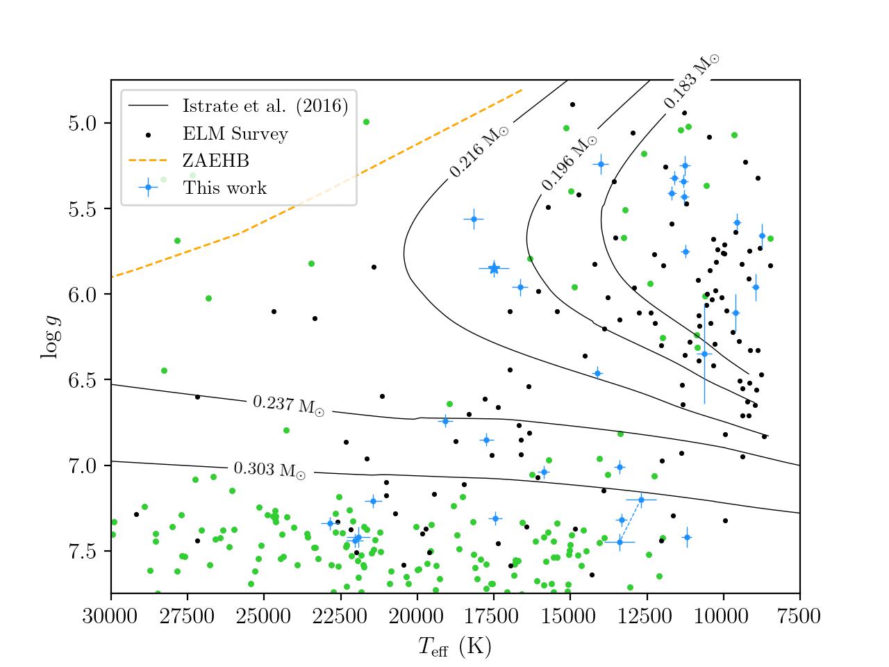
Figure 2: $\log{g}$-$T_{\rm eff}$ distribution of low mass white dwarfs identified as part of the ongoing ELM Survey. Previous ELM Survey binaries are displayed as black points. New binaries from this work are colored blue. Other objects observed as part of this work are colored green. We overplot the cooling tracks for $0.183~{}{\rm M_{\odot}}$, $0.196~{}{\rm M_{\odot}}$, $0.216~{}{\rm M_{\odot}}$, $0.237~{}{\rm M_{\odot}}$, and $0.303~{}{\rm M_{\odot}}$ white dwarfs with $Z=0.001$ from Istrate et al. (2016), including rotation and diffusion. We mark the location of the DABZ J2049$+$3351 with a blue star symbol and use a dashed line to connect the markers for the individual stars in the double-lined binary J2102$-$4145. The Zero-Age Extreme Horizontal Branch (ZAEHB) is colored as an orange dashed line for reference.

Object Name	R.A.	Decl.	$T_{\rm eff}$	$\log{g}$	$M_{1}$	${\rm Gaia}~{}G$	${\rm Gaia~{}Parallax}$
	(2016.0)	(2016.0)	($K$)	(${\rm cm~{}s^{-2}}$)	($M_{\odot}$)	(${\rm mag}$)	(${\rm mas}$)
J0135$+$2359	01:35:00.856	$+$23:59:46.091	$14130\pm 210$	$6.46\pm 0.05$	$0.21\pm 0.04$	$18.7$	$1.18\pm 0.29$
J0155$-$4148	01:55:34.866	$-$41:48:18.433	$11250\pm 170$	$5.75\pm 0.05$	$0.22\pm 0.02$	$15.7$	$2.08\pm 0.03$
J0215$+$015512	02:15:06.244	$+$01:55:03.363	$11310\pm 180$	$5.34\pm 0.05$	$0.29\pm 0.02$	$14.3$	$2.15\pm 0.03$
J0221$+$171012	02:21:10.832	$+$17:10:49.182	$13400\pm 200$	$7.01\pm 0.04$	$0.27\pm 0.01$	$17.7$	$3.58\pm 0.12$
J0256$+$4405	02:56:35.153	$+$44:05:27.363	$18170\pm 350$	$5.56\pm 0.06$	$0.22\pm 0.02$	$15.8$	$1.40\pm 0.04$
J0450$-$014512	04:50:13.108	$-$01:45:48.150	$9560\pm 140$	$5.58\pm 0.06$	$0.19\pm 0.02$	$17.7$	$0.91\pm 0.11$
J0501$-$231212	05:01:29.865	$-$23:12:04.397	$21440\pm 330$	$7.21\pm 0.05$	$0.36\pm 0.01$	$18.0$	$1.64\pm 0.10$
J0517$-$115312	05:17:24.974	$-$11:53:25.849	$16650\pm 300$	$5.96\pm 0.06$	$0.19\pm 0.02$	$16.2$	$1.47\pm 0.04$
J0545$-$1902	05:45:45.301	$-$19:02:45.499	$22850\pm 340$	$7.34\pm 0.05$	$0.40\pm 0.02$	$17.3$	$2.59\pm 0.07$
J0725$-$1245	07:25:27.362	$-$12:45:46.824	$21920\pm 420$	$7.42\pm 0.06$	$0.42\pm 0.02$	$18.9$	$1.51\pm 0.25$
J1121$+$605210	11:21:57.163	$+$60:52:10.265	$11690\pm 170$	$5.41\pm 0.05$	$0.19\pm 0.01$	$16.0$	$1.33\pm 0.04$
J1129$+$471512	11:29:14.162	$+$47:15:01.726	$11610\pm 170$	$5.32\pm 0.05$	$0.19\pm 0.01$	$16.1$	$1.18\pm 0.04$
J1240$-$0958	12:40:32.501	$-$09:58:59.603	$14020\pm 280$	$5.24\pm 0.06$	$0.20\pm 0.02$	$19.0$	$1.30\pm 0.30$
J1255$-$1853	12:55:39.147	$-$18:53:32.101	$11270\pm 200$	$5.25\pm 0.06$	$0.19\pm 0.01$	$17.8$	$0.55\pm 0.13$
J1459$-$1920	14:59:02.159	$-$19:20:33.552	$8740\pm 130$	$5.66\pm 0.07$	$0.26\pm 0.02$	$18.1$	$0.71\pm 0.16$
J1506$-$1125	15:06:12.345	$-$11:25:11.994	($22050\pm 320$)	($7.44\pm 0.05$)	($0.43\pm 0.02$)	$17.0$	$2.42\pm 0.10$
J1526$-$271112	15:26:01.115	$-$27:11:56.660	$17460\pm 260$	$7.31\pm 0.05$	$0.37\pm 0.02$	$18.3$	$1.61\pm 0.18$
J1553$+$673612	15:53:28.008	$+$67:36:10.560	$9610\pm 150$	$6.11\pm 0.11$	$0.22\pm 0.04$	$16.5$	$2.36\pm 0.04$
J1555$+$100712	15:55:15.894	$+$10:07:24.851	$13340\pm 220$	$7.32\pm 0.05$	$0.35\pm 0.02$	$18.2$	$2.52\pm 0.15$
J1657$-$0417	16:57:24.888	$-$04:17:22.348	$17750\pm 270$	$6.85\pm 0.05$	$0.27\pm 0.02$	$18.3$	$2.04\pm 0.18$
J1808$+$2723	18:08:38.994	$+$27:23:12.216	$10630\pm 270$	$6.35\pm 0.29$	$0.22\pm 0.04$	$15.5$	$2.82\pm 0.03$
J1812$+$052511	18:12:38.471	$+$05:25:29.868	$8960\pm 130$	$5.96\pm 0.08$	$0.28\pm 0.03$	$18.9$	$0.85\pm 0.26$
J1832$+$203112	18:32:36.539	$+$20:31:08.202	$19080\pm 290$	$6.74\pm 0.05$	$0.29\pm 0.03$	$17.6$	$1.61\pm 0.08$
J2013$-$131012	20:13:53.498	$-$13:10:41.750	$11200\pm 190$	$7.42\pm 0.06$	$0.37\pm 0.02$	$18.7$	$2.21\pm 0.25$
J2049$+$335111	20:49:51.274	$+$33:51:53.126	$17500\pm 500$	$5.85\pm 0.05$	$\cdots$	$18.7$	$0.51\pm 0.16$
J2102$-$4145a10	21:02:20.456	$-$41:45:01.736	$12700\pm 500$	$7.20\pm 0.05$	$0.32\pm 0.01$	$15.8$	$6.07\pm 0.04$
J2102$-$4145b10	21:02:20.456	$-$41:45:01.736	$13400\pm 500$	$7.45\pm 0.05$	$0.39\pm 0.01$	$\cdots$	$6.07\pm 0.04$
J2243$-$4511	22:43:27.479	$-$45:11:18.404	$15880\pm 230$	$7.04\pm 0.05$	$0.29\pm 0.01$	$17.4$	$2.57\pm 0.09$
J2303$-$26141012	23:03:23.542	$-$26:14:59.917	$11280\pm 160$	$5.43\pm 0.05$	$0.18\pm 0.01$	$13.8$	$3.12\pm 0.02$

Table 1: White dwarf parameters determined through optical spectroscopy for the 28 new binaries identified in this work. Our reported atmospheric parameters $T_{\rm eff}$ and $\log{g}$ include the external uncertainties of $\sigma_{T_{\rm eff}}=1.4\%$ and $\sigma_{\log{g}}=0.042~{}{\rm dex}$ from Liebert et al. (2005). Binaries which show photometric variability in the TESS 2$-$minute cadence or ZTF data archives are marked. We apply 3D corrections using the equations from Tremblay et al. (2015) for objects cooler than $T_{\rm eff}\approx 10000~{}{\rm K}$. The atmospheric parameter values for J1506$-$1125 displayed in this table are based on single-star models. We describe our multi-component modeling to J1506$-$1125 in Section 6, which does not identify a unique solution.

Object Name	$P$	$K$	$\gamma$	$M_{\rm 2}$	$\tau_{\rm merge}$	Disk
	(${\rm days}$)	(${\rm km~{}s^{-1}}$)	(${\rm km~{}s^{-1}}$)	($M_{\odot}$)	(${\rm Gyr}$)
J0135$+$2359	$1.177655\pm 0.009923$	$178.9\pm 6.4$	$-35.7\pm 6.2$	$>1.02\pm 0.09$	$<371.4\pm 71.7$	1
J0155$-$4148	$0.343865\pm 0.000317$	$220.4\pm 3.7$	$-4.0\pm 2.9$	$>0.67\pm 0.03$	$<18.1\pm 1.6$	1
J0215$+$015512	$0.387941\pm 0.000001$	$186.4\pm 1.5$	$-49.4\pm 1.1$	$>0.58\pm 0.02$	$<21.7\pm 1.4$	0
J0221$+$171012	$0.061288\pm 0.000020$	$347.9\pm 4.2$	$35.3\pm 3.7$	$0.58\pm 0.02$	$0.17\pm 0.01$	1
J0256$+$4405	$0.261260\pm 0.000087$	$243.7\pm 3.8$	$28.1\pm 2.9$	$>0.68\pm 0.03$	$<8.6\pm 0.8$	1
J0450$-$014512	$0.192169\pm 0.000040$	$260.2\pm 3.3$	$65.5\pm 2.9$	$>0.61\pm 0.02$	$<4.7\pm 0.5$	1
J0501$-$231212	$0.086593\pm 0.001156$	$105.1\pm 5.1$	$6.3\pm 7.2$	$>0.14\pm 0.01$	$<1.1\pm 0.1$	1
J0517$-$115312	$0.250521\pm 0.000001$	$309.7\pm 3.1$	$53.5\pm 2.6$	$>1.07\pm 0.04$	$<6.3\pm 0.7$	1
J0545$-$1902	$0.144472\pm 0.000684$	$134.7\pm 5.4$	$146.1\pm 5.7$	$>0.25\pm 0.02$	$<2.4\pm 0.2$	1
J0725$-$1245	$0.106135\pm 0.000061$	$79.6\pm 5.0$	$90.4\pm 3.2$	$>0.12\pm 0.01$	$<2.0\pm 0.2$	1
J1121$+$605210	$0.084511\pm 0.000013$	$183.5\pm 2.6$	$-15.7\pm 2.2$	$>0.20\pm 0.01$	$<1.3\pm 0.1$	1
J1129$+$471512	$0.238823\pm 0.000032$	$185.8\pm 4.4$	$40.9\pm 3.0$	$>0.37\pm 0.02$	$<12.4\pm 0.7$	1
J1240$-$0958	$0.400383\pm 0.002945$	$209.8\pm 6.1$	$23.9\pm 3.3$	$>0.65\pm 0.04$	$<30.3\pm 3.2$	1
J1255$-$1853	$0.363739\pm 0.001501$	$230.8\pm 6.2$	$-15.2\pm 29.5$	$>0.73\pm 0.04$	$<22.6\pm 1.5$	1
J1459$-$1920	$0.151990\pm 0.000030$	$287.8\pm 7.4$	$45.6\pm 5.0$	$>0.70\pm 0.04$	$<1.7\pm 0.1$	0
J1506$-$1125	$0.032320\pm 0.000390$	$167.5\pm 4.3$	$43.5\pm 2.8$	$>0.18\pm 0.01$	$<0.056\pm 0.003$	1
J1526$-$271112	$0.027982\pm 0.000439$	$336.0\pm 5.6$	$8.4\pm 4.8$	$>0.40\pm 0.02$	$<0.021\pm 0.001$	1
J1553$+$673612	$0.174522\pm 0.000431$	$91.6\pm 5.4$	$10.9\pm 6.1$	$>0.12\pm 0.01$	$<12.4\pm 2.3$	1
J1555$+$100712	$0.298037\pm 0.000877$	$148.5\pm 6.7$	$-51.4\pm 3.7$	$>0.38\pm 0.03$	$<13.0\pm 1.0$	1
J1657$-$0417	$0.083954\pm 0.000441$	$289.4\pm 8.8$	$-69.8\pm 21.3$	$>0.50\pm 0.03$	$<0.44\pm 0.04$	1
J1808$+$2723	$0.098787\pm 0.000053$	$187.2\pm 3.0$	$-69.3\pm 1.9$	$>0.24\pm 0.02$	$<1.4\pm 0.2$	1
J1812$+$052511	$0.059847\pm 0.000083$	$373.3\pm 6.2$	$-139.6\pm 4.7$	$0.73^{+0.05}_{-0.04}$	$0.13\pm 0.01$	0
J1832$+$203112	$0.046641\pm 0.000002$	$335.2\pm 4.2$	$-37.4\pm 3.3$	$>0.47\pm 0.02$	$<0.090\pm 0.009$	1
J2013$-$131012	$0.061618\pm 0.000597$	$300.9\pm 6.5$	$-40.2\pm 6.3$	$>0.51\pm 0.02$	$<0.14\pm 0.01$	1
J2049$+$335111	$0.029747\pm 0.000007$	$513.2\pm 9.5$	$-3.4\pm 7.7$	$\cdots$	$\cdots$	1
J2102$-$4145a10	$0.117631\pm 0.003244$	$227^{+8}_{-6}$	$-7.9^{+7.1}_{-5.8}$	$\cdots$	$<0.74\pm 0.02$	1
J2102$-$4145b10	$0.117631\pm 0.003244$	$186^{+8}_{-7}$	$-18.7^{+6.2}_{-7.0}$	$\cdots$	$<0.74\pm 0.02$	1
J2243$-$4511	$0.109479\pm 0.000043$	$249.4\pm 4.9$	$6.0\pm 3.7$	$>0.46\pm 0.02$	$<0.89\pm 0.04$	1
J2303$-$26141012	$0.118195\pm 0.000032$	$302.9\pm 2.3$	$-17.1\pm 2.1$	$>0.58\pm 0.01$	$<1.4\pm 0.1$	1

Table 2: Orbital solutions to the 28 new low mass white dwarf binaries presented in this work.

J0215$+$0155

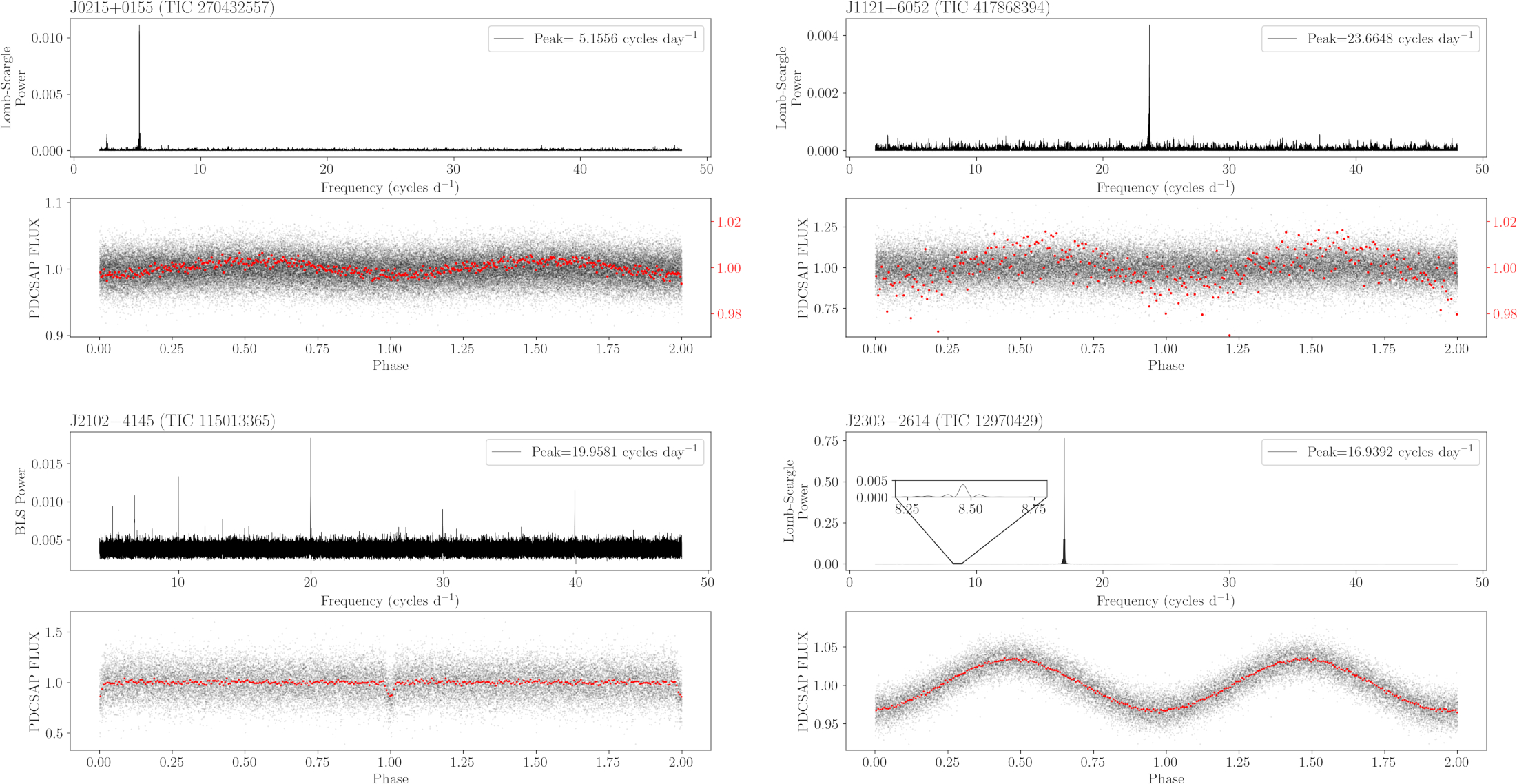
Figure 3: Lomb-Scargle or Box Least Squares (BLS) power spectrum (top) and its TESS 2-minute cadence light curve (bottom) for J0215$+$0155 (TIC 270432557; upper-left), J1121$+$6052 (TIC 417868394; upper-right), J2102$-$4145 (TIC 115013365; lower-left), and J2303$-$2614 (TIC 12970429; lower-right). Red data points represent the original data binned by 100. We re-scaled the binned data of J0215$+$0155 and J1121$+$6052 to emphasize the variability seen at the 1% level.

We obtained 112 radial velocity measurements for J021506.244$+$015503.363 (J0215$+$0155; GAIA DR3 2513538251735261696), resulting in best-fitting orbital parameters $P_{\rm RV}=9.3106~{}{\rm h}$, $K=186.4\pm 1.5~{}{\rm km~{}s^{-1}}$, and $\gamma=-49.4\pm 1.1~{}{\rm km~{}s^{-1}}$. Together with Gaia DR3 astrometry, we estimated the Galactic space velocities $[U,V,W]=[121\pm 1,-37\pm 1,-59\pm 1]~{}{\rm km~{}s^{-1}}$, ($U$ positive towards the Galactic center), corrected for the motion of the local standard of rest (Schönrich et al., 2010).

We determine Galactic disk and halo membership by computing the Mahalanobis distance between the measured Galactic space velocities and the velocity distributions for thick disk and halo populations using average velocities and velocity dispersions from (Chiba & Beers, 2000). Specifically, we compared against velocity distributions defined by $[\langle U\rangle,\langle V\rangle,\langle W\rangle]_{\rm Disk}=[4\pm 46,-20\pm 50,-3\pm 35]~{}{\rm km~{}s^{-1}}$ and $[\langle U\rangle,\langle V\rangle,\langle W\rangle]_{\rm Halo}=[17\pm 141,-187\pm 106,-5\pm 94]~{}{\rm km~{}s^{-1}}$ for the thick disk and halo, respectively. Our measurements for J0215$+$0155 are consistent with Galactic halo membership.

Our pure-hydrogen model atmosphere fits to the summed zero-velocity spectrum of J0215$+$0155 result in best-fitting atmospheric parameters $T_{\rm eff}=11{\rm,}310\pm 180~{}{\rm K}$ and $\log{g}=5.34\pm 0.05$, corresponding to white dwarf with mass $M_{1}=0.29\pm 0.02~{}{\rm M_{\odot}}$ based on the halo metallicity models for He-core white dwarfs from Istrate et al. (2016). With the velocity semi-amplitude known and orbital period known, we used the binary mass function,

$$\frac{(M_{2}\sin{i})^{3}}{(M_{1}+M_{2})^{2}}=\frac{PK^{3}}{2\pi G}$$ (1)

to estimate the minimum companion mass $M_{\rm 2,min}=0.59\pm 0.02~{}{\rm M_{\odot}}$.

We find three sectors of TESS 2-minute cadence data for J0215$+$0155 (TIC 270432557). Our Lomb Scargle algorithm identifies weak ($\sim 1\%$ level) periodic variability at $f_{\rm TESS}=5.1556~{}{\rm cycles~{}d^{-1}}$, equal to half of the orbital period determined through radial velocity measurements. Figure 3 (upper-left) displays the phase-folded TESS light curve of J0215$+$0155 and its Lomb Scargle power spectrum. A smaller peak can be seen in the power spectrum at the true orbital frequency of the system. The dominant frequency at $5.1556~{}{\rm cycles~{}d^{-1}}$ is likely caused by tidal distortions in the compact binary. Detailed high-precision follow-up light curve analysis may help place constraints on the orbital inclination and mass ratio of this binary, (see, for example, Hermes et al., 2014).

J0221$+$1710

We obtained 19 radial velocity measurements of J022110.832$+$171049.182 (J0221$+$1710; GAIA DR3 79808158877017216), resulting in orbital parameters $P_{\rm RV}=1.4709\pm 0.0005~{}{\rm h}$, $K=347.9\pm 4.2~{}{\rm km~{}s^{-1}}$, $\gamma=35.3\pm 3.7~{}{\rm km~{}s^{-1}}$. With precise Gaia astrometry, we estimated Galactic space velocities $[U,V,W]=[-40.4\pm 1.8,-4.8\pm 1.6,7.5\pm 1.7]~{}{\rm km~{}s^{-1}}$, which are well within the $2\sigma$ velocity ellipsoid for the Galactic disk.

Our best-fitting pure-hydrogen atmospheric parameters to J0221$+$1710 are $T_{\rm eff}=13{\rm,}400\pm 200~{}{\rm K}$ and $\log{g}=7.01\pm 0.04$, corresponding to a white dwarf with mass $M_{1}=0.27\pm 0.01~{}{\rm M_{\odot}}$, based on the ${\rm Z}=0.02$ model tracks of Istrate et al. (2016).

Our BLS periodicity search on the ZTF DR13 data archive identified periodic $\Delta m\approx 0.2~{}{\rm mag}$ eclipses at $P_{\rm ZTF,BLS}=88.2508~{}{\rm min}$ ($1.4708~{}{\rm h}$), in agreement with our orbital period obtained through radial velocity measurements.

We obtained high-speed $g$- and $r$-band photometry using the McDonald 2.1-meter telescope on UT 20221001 and UT 20221002. Our observations cover three eclipses in each filter. We used ${\rm EXPTIME}=10~{}{\rm s}$, resulting in five mid-eclipse data points and four data points during the ingress or egress per eclipse for the $\approx 90~{}{\rm s}$ eclipse duration.

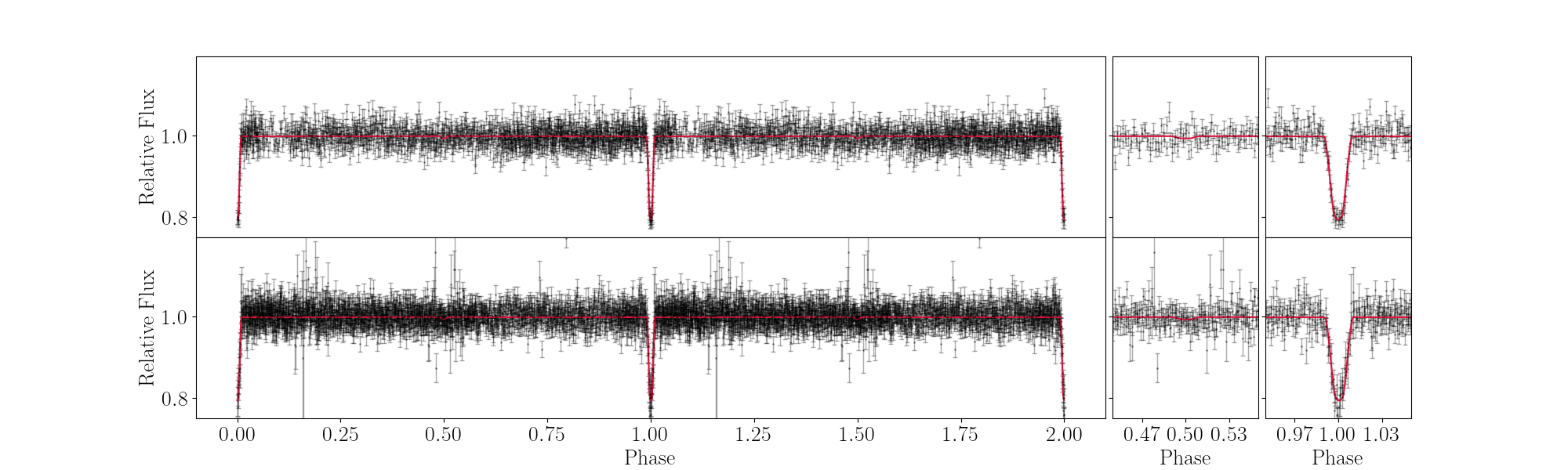
Figure 4: McDonald 2.1-meter $g$-band (top) and $r$-band (bottom) light curves of J0221$+$1710. Best-fitting lcurve models are overplotted in red. We provide zoomed-in subplots showing the regions surrounding the primary and secondary eclipses.

	J0221$+$1710	J1812$+$0525	J2049$+$3351
$q$	$\cdots$	$0.41\pm 0.03$	$0.39\pm 0.2$
$i~{}({\rm{}^{\circ}})$	$89.0\pm 0.2$	$75^{+2}_{-5}$	$74^{+3}_{-2}$
$R_{1}/a$	$0.045\pm 0.001$	$0.20\pm 0.01$	$0.31\pm 0.05$
$R_{2}/a$	$0.020\pm 0.001$	$\cdots$	$0.06^{+0.03}_{-0.02}$
$T_{\rm eff,1}~{}({\rm K})$	$13400\pm 180$	$8900\pm 100$	$23200^{+4900}_{-4300}$
$T_{\rm eff,2}~{}({\rm K})$	$\lesssim 6400$	$\cdots$	$35400^{+9700}_{-8600}$

Table 3: System parameters for J0211$+$1710, J1812$+$0525, and J2049$+$3351, obtained through light curve modeling with lcurve as described in the text.

We modeled the geometry of the binary by simultaneously fitting the $g$- and $r$-band light curves using lcurve (Copperwheat et al., 2010), fitting for the component radii ($r_{i}=\frac{R_{i}}{a}$) and the temperature of the companion ($T_{\rm eff,2}$). We fixed the orbital period to the value obtained from our ZTF BLS analysis and used the results from our spectroscopic follow-up ($T_{\rm eff,1}$, $\log{g_{1}}$, and $K_{1}$) as Gaussian priors to our light curve modeling. We interpolated over the grid of gravity darkening and quadratic limb darkening coefficients from Claret et al. (2020) for our primary star based on our spectroscopic values and used values for a companion with $T_{\rm eff,2}=10{\rm,}000~{}{\rm K}$ and $\log{g_{2}}=8.0$.

The most probable system parameters from our light curve fitting are $R_{1}=0.028\pm 0.001~{}{\rm R_{\odot}}$, $R_{2}=0.012\pm 0.001~{}{\rm R_{\odot}}$, $i=89.0\pm 0.2^{\circ}$, and $T_{\rm eff,2}=5200^{+400}_{-500}~{}{\rm K}$. However, given the quality of our McDonald $r$-band light curve data during the eclipse, we adopt the 3-sigma upper limit to the temperature of the companion. Our most probable model parameters are summarized in Table 3. Figure 4 displays our phase-folded McDonald 2.1-meter $g$- (top) and $r$-band (bottom) light curves with the best-fitting model over-plotted in red.

With the inclination and radial velocity semi-amplitude known, we used the binary mass function to calculate the companion mass $M_{2}=0.58\pm 0.02~{}{\rm M_{\odot}}$, corresponding to radius $R_{2}=0.0129~{}{\rm R_{\odot}}$, in agreement with the radius estimate from our light curve modeling.

We similarly fit our eclipsing $g$- and $r$-band light curves for J0221$+$1710 separately using jktebop (Southworth et al., 2004; Southworth, 2013) to confirm the consistency of our lcurve solution. We fit for the sum and ratio of the component radii, the inclination, and the surface brightness ratio. We performed 10,000 Monte Carlo iterations, which returned a solution degenerate in inclination ($88.6\pm 0.2^{\circ}$ and $87.9\pm 0.2^{\circ}$). The most probable degenerate solution agrees well with our lcurve results, returning: $R_{1}=0.029\pm 0.001~{}{\rm R_{\odot}}$, $R_{2}=0.013\pm 0.001~{}{\rm R_{\odot}}$, $i=88.6\pm 0.2^{\circ}$, and $T_{\rm eff,2}\approx 6200~{}{\rm K}$ We report our simultaneous $g$- and $r$-band solution from the lcurve solution as the true system parameters of J0221$+$1710.

With the individual component masses, orbital period, and orbital inclination known, we estimated the gravitational wave strain using the equation

$$h_{c}=3.4\times 10^{-23}\frac{\mathcal{M}^{5/3}\sqrt{\cos^{4}{i}+2\cos^{2}{i}+1}}{P^{2/3}~{}d},$$ (2)

where $\mathcal{M}$ is the chirp mass, $P$ is the period in days, and $d$ is the distance in kpc (Timpano et al., 2006; Roelofs et al., 2007). We multiplied by $\sqrt{(4~{}{\rm yr})f_{\rm GW}}$ to account for the increased signal after a 4-year LISA mission. Our estimated gravitational wave strain for J0221$+$1710 is $h_{c}=(2.87\pm 0.14)\times 10^{-20}$. Additionally, we estimated the orbital decay due to gravitational wave emission using the equation

$$\dot{P}=\frac{96}{5}\left(\frac{G\mathcal{M}}{P}\right)^{5/3}\frac{2\pi}{c^{5}},$$ (3)

resulting in $\dot{P}=(3.86\pm 0.14)\times 10^{-14}~{}{\rm s~{}s^{-1}}$, which corresponds to an eclipse timing offset of $\Delta T_{0}\approx-3.6\pm 0.1~{}{\rm s}$ after 10 years.

J1121$+$6052

Our 26 radial velocity measurements of J112157.163$+$605210.265 (J1121$+$6052; GAIA DR3 861011995046220544) return best-fitting orbital parameters $P_{\rm RV}=2.0283\pm 0.0003~{}{\rm h}$, $K=183.5\pm 2.6~{}{\rm km~{}s^{-1}}$, and $\gamma=-15.7\pm 2.2~{}{\rm km~{}s^{-1}}$. We calculated the Galactic space velocities $[U,V,W]=[56.7\pm 1.4,-10.2\pm 1.5,23.4\pm 1.4]~{}{\rm km~{}s^{-1}}$, consistent with a short-period binary in the disk.

Our pure-hydrogen atmosphere fits to the summed zero-velocity spectrum of J1121$+$6052 resulted in atmospheric parameters $T_{\rm eff}=11{\rm,}690\pm 170~{}{\rm K}$ and $\log{g}=5.41\pm 0.05$, which suggests white dwarf mass $M_{1}=0.19\pm 0.01~{}{\rm M_{\odot}}$ based on the ${\rm Z}=0.02$ model tracks of Istrate et al. (2016).

We find a weak periodic signal in the TESS 2-minute cadence data through our Lomb-Scargle periodicity search of J1121$+$6052 (TIC 417868394). The TESS light curve shows periodic variability at the 1% level with frequency $f_{\rm TESS}=23.6649~{}{\rm cycles~{}d^{-1}}$ ($P_{\rm TESS}=1.0142~{}{\rm h}$); half the period obtained through radial velocity measurements. We display the phase-folded TESS 2-minute cadence light curve in Figure 3 (upper-right). J1121$+$6042 is in a relatively isolated field, with no nearby bright stars to heavily dilute the TESS light curve. We do not recover this weak periodic signal in the available ground-based ZTF data.

J1506$-$1125

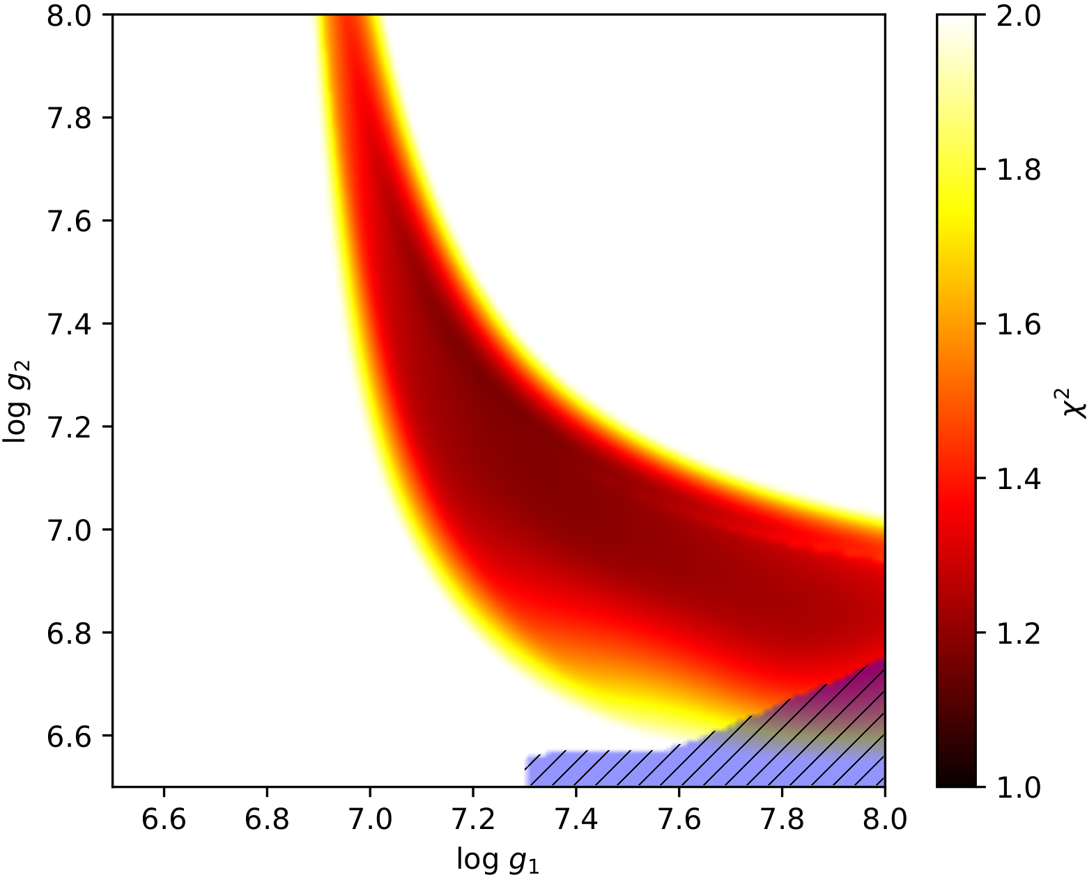
Figure 5: Normalized $\chi^{2}$ distribution from our fits to the combined SED and optical spectroscopy for J1506$-$1125, as a function of $\log{g_{1}}$ and $\log{g_{2}}$. The hatched blue region represents the region of parameter space excluded by constraints from the binary mass function.

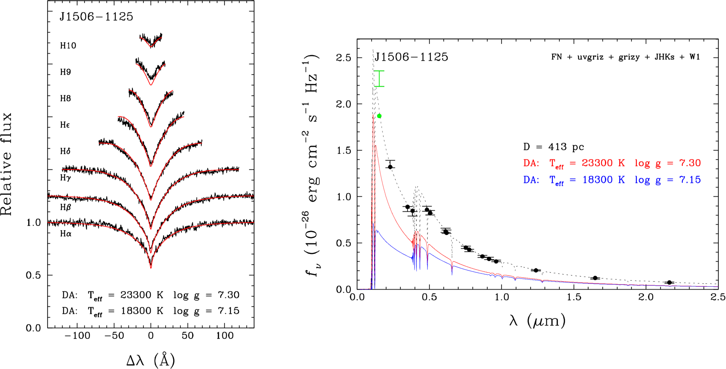
Figure 6: Example model-atmosphere fit to the spectrum (left) and SED (right) of J1506$-$1125 including contributions from two DA white dwarfs. In the left panel, the observed and predicted Balmer lines are shown as black and red lines, respectively. In the right panel, the observed and predicted average fluxes are displayed as error bars and filled circles, respectively; for reference, the red and blue lines show the individual contributions of the components to the total monochromatic model flux, which is displayed as a black dotted line. The GALEX FUV photometry measurement (green) is excluded from our SED fit. This fit does not represent a unique solution (see text).

We obtained 31 radial velocity measurements for J150612.345$-$112511.994 (J1506$-$1125; Gaia DR3 6312837970697953920). Our best-fitting circular orbit fits suggest orbital parameters $P_{\rm RV}=0.7757\pm 0.0094~{}{\rm h}$, $K=167.5\pm 4.3~{}{\rm km~{}s^{-1}}$, and $\gamma=43.5\pm 2.8~{}{\rm km~{}s^{-1}}$. J1506$-$1125 is likely a disk object with Galactic space velocities $[U,V,W]=[41.8\pm 1.6,-7.3\pm 1.5,13.3\pm 1.4]~{}{\rm km~{}s^{-1}}$.

Our pure-hydrogen model atmosphere fits to the summed zero-velocity spectrum result in best-fitting atmospheric parameters $T_{\rm eff}=22{\rm,}050\pm 320~{}{\rm K}$ and $\log{g}=7.44\pm 0.05$, which corresponds to a white dwarf with mass $M_{1}=0.43\pm 0.02~{}{\rm M_{\odot}}$ based on disk-metallicity models of Althaus et al. (2013). Our radial velocity measurements suggest a minimum companion mass $M_{\rm 2,min}=0.18\pm 0.01~{}{\rm M_{\odot}}$, significantly below the mass of the visible star.

Interestingly, our distance estimates suggest that J1506$-$1125 is over-luminous when compared to our single-star SED models, which suggests our single-star atmospheric model parameters may be inaccurate due to significant contribution to the system light from a companion. However, given the relatively low radial velocity semi-amplitude ($K=167.5\pm 4.3~{}{\rm km~{}s^{-1}}$), we are not able to resolve individual absorption components in our Magellan 6.5-meter optical spectrum with $\approx 1.0~{}{\rm\AA}$ resolution, if they are present.

We performed simultaneous model atmosphere fits to the SED and median-combined optical spectrum of J1506$-$1125, including contribution from two components in a binary (see Bédard et al., 2017; Kilic et al., 2020, for the details of the method). The SED was built from the available GALEX (NUV; Martin et al., 2005), SkyMapper (uvgriz; Onken et al., 2019), Pan-STARRS (grizy; Chambers et al., 2016), 2MASS (JH${\rm K_{s}}$; Skrutskie et al., 2006), and AllWISE (W1; Wright et al., 2010; Mainzer et al., 2011) photometry, and dereddened using the extinction maps of Schlafly & Finkbeiner (2011). Figure 5 shows the resulting $\chi^{2}$ distribution plot as a function of $\log{g_{1}}$ and $\log{g_{2}}$, with the region of parameter space excluded by constraints from the binary mass function shaded in blue. Dark regions indicate the regions with the most probable system parameters based on our fits.

Because we do not resolve individual absorption components in our optical spectrum, we are unable to identify a unique solution to describe the atmospheric parameters of the components of J1506$-$1125. Figure 6 displays an example fit near the center of the dark region, defined by $T_{\rm eff,1}=23{\rm,}300~{}{\rm K}$, $\log{g_{1}}=7.30$, $T_{\rm eff,2}=18{\rm,}300~{}{\rm K}$ and $\log{g_{2}}=7.15$, corresponding to masses $M_{1}=0.40~{}{\rm M_{\odot}}$ and $M_{2}=0.33~{}{\rm M_{\odot}}$ based on He-core cooling tracks of Althaus et al. (2013). However, the extremes of our probable parameter space allow for solutions at [($T_{\rm eff,1}$,$T_{\rm eff,2}$), ($\log{g_{1}}$,$\log{g_{2}}$), ($M_{1}$,$M_{2}$)] = [($22{\rm,}000~{}{\rm K}$, $18{\rm,}100~{}{\rm K}$), ($7.05$, $7.55$), ($0.34~{}{\rm M_{\odot}}$, $0.43~{}{\rm M_{\odot}}$)] and [($27{\rm,}300~{}{\rm K}$, $17{\rm,}900~{}{\rm K}$), ($7.80$, $6.90$), ($0.54~{}{\rm M_{\odot}}$, $0.28~{}{\rm M_{\odot}}$)], where we used C/O-core cooling tracks of Bédard et al. (2020) for the relatively massive $0.54~{}{\rm M_{\odot}}$ solution.

We find no TESS Full-Frame image data, 2-minute cadence data, or 20-second cadence data for J1506$-$1125 up to sector 56. Our Lomb-Scargle and BLS algorithms do not identify periodic photometric variability in the public ZTF DR13 data archive.

J1812$+$0525

The orbital period of J181238.471$+$052529.868 (J1812$+$0525; Gaia DR3 4471573464995153280) was constrained through its periodic photometric variability identified in our search of the public ZTF data archive. Our Lomb Scargle periodogram identified periodic photometric variability at $P_{\rm ZTF}=43.1~{}{\rm min}$.

We obtained a single follow-up spectrum on 2022 June 03 to confirm its nature. We then completed its orbital solution with seven additional back-to-back spectra during the following night. Figure 7 (left) displays our orbital solution for J1812$+$0525. Our best-fitting radial velocity solution finds velocity semi-amplitude $K=373.3\pm 6.2~{}{\rm km~{}s^{-1}}$, systemic velocity $\gamma=-139.6\pm 4.7~{}{\rm km~{}s^{-1}}$, and orbital period $P_{\rm RV}=1.436\pm 0.002~{}{\rm h}$ ($86.2\pm 0.1~{}{\rm min}$), in good agreement with the half-period identified from the ZTF data. We use the precise Gaia DR3 astrometry, together with our radial velocity information, to estimate its Galactic velocities $[U,V,W]=[-92.9\pm 2.3,-87.4\pm 2.8,-1.1\pm 2.4]~{}{\rm km~{}s^{-1}}$, which suggests that J1812$+$0525 is a short-period binary in the Galactic Halo.

We fit the summed zero-velocity spectrum with pure-hydrogen model atmospheres and obtained best-fitting atmospheric parameters $T_{\rm eff,0}=9300\pm 120~{}{\rm K}$ and $\log{g_{0}}=6.11\pm 0.05$. Because this is a cool object, we corrected its atmospheric solution for 3D effects using equations provided in Tremblay et al. (2015), resulting in corrected atmospheric parameters $T_{\rm eff}=8960\pm 130~{}{\rm K}$ and $\log{g}=5.96\pm 0.08$, corresponding to a primary mass $M_{1}=0.28\pm 0.03~{}{\rm M_{\odot}}$ based on the halo-metallicity models tracks of Istrate et al. (2016).

We used the McDonald Observatory 2.1-meter telescope to confirm photometric variability at $P=43.4~{}{\rm min}$, roughly consistent with the half-period seen in the public ZTF data. However, our data quality is too poor to reasonably constrain orbital parameters through photometric fitting.

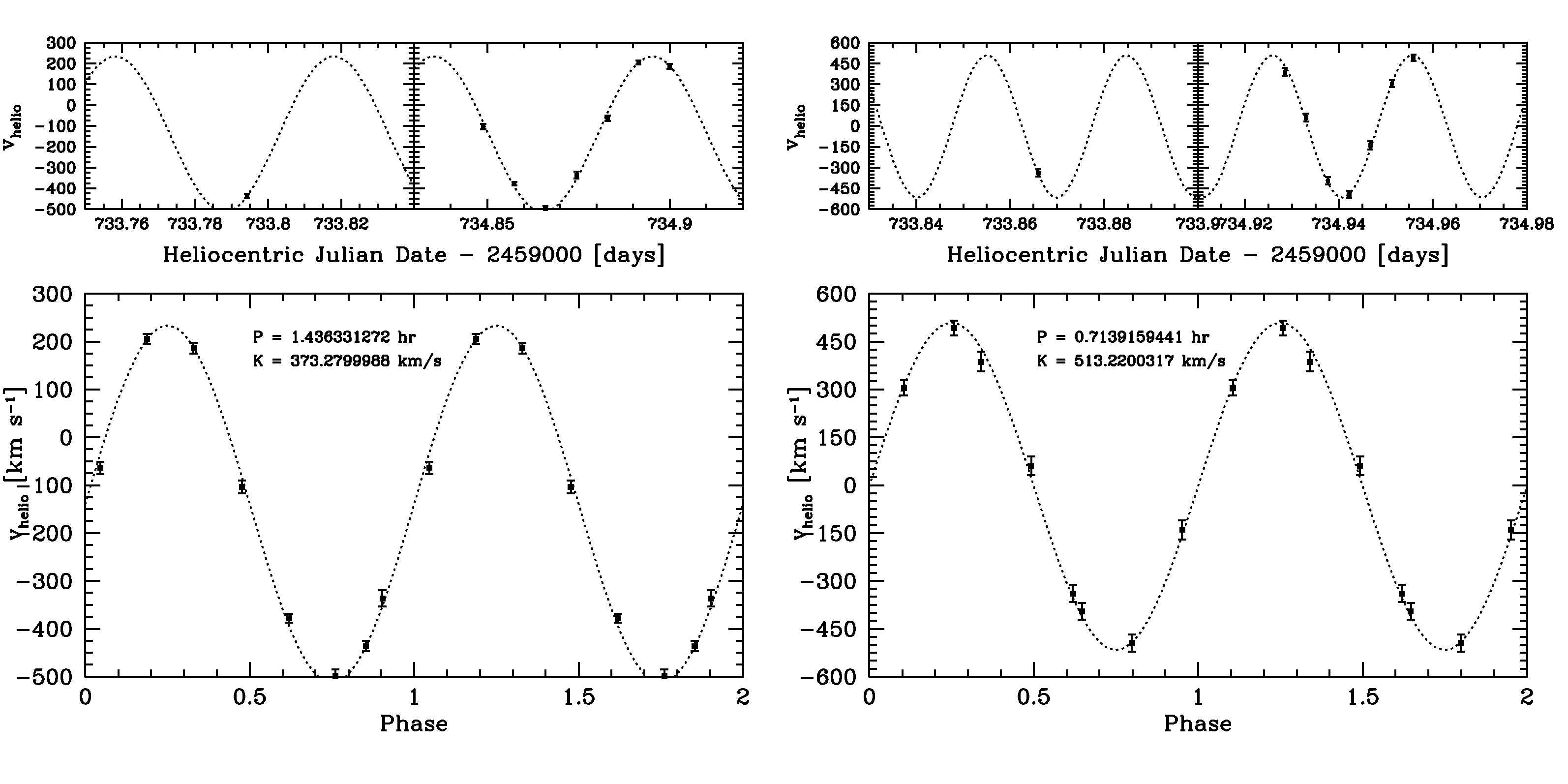
Figure 7: Orbital solutions for J1812$+$0525 (left) and J2049$+$3351 (right).

We instead modelled the ZTF DR16 $g$- and $r$-band data simultaneously using lcurve. Our free parameters included the mass ratio ($q=\frac{M_{1}}{M_{2}}<1.0$), scaled primary star radius ($r_{1}=\frac{R_{1}}{a}$), orbital inclination ($i$), primary star effective temperature ($T_{\rm eff,1}$), time of superior conjunction ($t_{0}$), and the velocity scale (the sum of the unprojected orbital speeds). We fixed the gravity and quadratic limb-darkening coefficients to values from Claret et al. (2020) for a $T_{\rm eff,1}=9000~{}{\rm K}$, $\log{g_{1}}=6.0$ primary with a $T_{\rm eff,2}=5500~{}{\rm K}$, $\log{g_{1}}=8.0$ companion and assign Gaussian priors based on our spectroscopic values for $T_{\rm eff,1}$, $\log{g_{1}}$, and $K_{1}$. The most-probable system parameters based on our light curve modelling are $q=0.42\pm 0.03$, $r_{1}=0.20\pm 0.01$, $i=75^{+2}_{-5}~{}^{\circ}$, and $T_{\rm eff,1}=8900\pm 100~{}{\rm K}$. These parameters are summarized in Table 3. With constraints from our radial velocity measurements, this corresponds to an $M_{1}=0.30\pm 0.03~{}{\rm M_{\odot}}$ primary star with an $M_{2}=0.73^{+0.05}_{-0.04}~{}{\rm M_{\odot}}$ companion.

J2049$+$3351

The orbital period of J204951.274$+$335153.126 (J2049$+$3351; Gaia DR3 1869111286948848128) was constrained through its periodic photometric variability identified in our search of the public ZTF data archive. Our Lomb Scargle algorithm identified strong variability at $P_{\rm ZTF}=21.6~{}{\rm min}$ with amplitude $A\approx 0.07~{}{\rm mag}$.

We obtained a single follow-up spectrum on 2022 June 03 to confirm its nature and completed its orbital solution with seven additional back-to-back spectra on the following night. Figure 7 (right) displays our orbital solution for J2049$+$3351. Our best-fitting radial velocity solution yields velocity semi-amplitude $K=513.2\pm 9.5~{}{\rm km~{}s^{-1}}$, systemic velocity $\gamma=-3.4\pm 7.7~{}{\rm km~{}s^{-1}}$, and orbital period $P_{\rm RV}=0.7139\pm 0.0002~{}{\rm h}$ ($42.834\pm 0.012~{}{\rm min}$), in good agreement with the half-period identified from the ZTF data. The Galactic space velocities, $[U,V,W]=[-9.8\pm 2.4,-8.1\pm 2.6,13.4\pm 2.3]~{}{\rm km~{}s^{-1}}$, place J2049$+$3351 in the Galactic disk.

J2049$+$3351 has an interesting optical absorption spectrum, including broad Hydrogen Balmer lines with strong He I absorption at $4472~{}{\rm\AA}$, $4388~{}{\rm\AA}$, $4143~{}{\rm\AA}$, and $4026~{}{\rm\AA}$, as well as a weak Ca II feature at $3933~{}{\rm\AA}$. Our MMT 6.5-meter optical spectrum of J2049$+$3351 is presented in Figure 8. We note that the individual Hydrogen and Helium absorption lines appear to move in-sync with each other throughout the orbit of the binary.

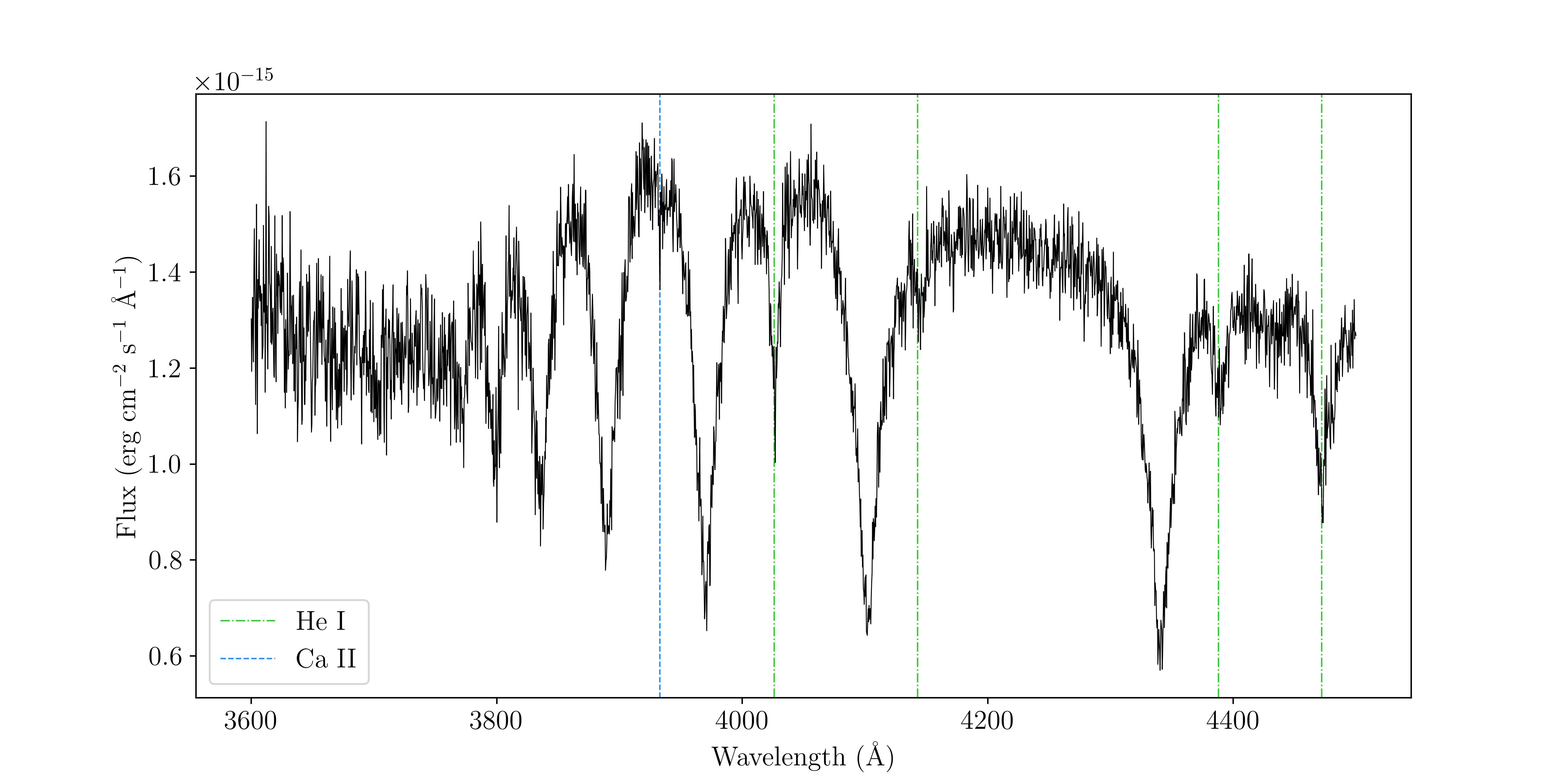
Figure 8: Co-added MMT optical spectrum of J2049$+$3351. In addition to the dominant Hydrogen Balmer absorption, strong neutral Helium absorption features (green dash-dot lines) can be seen at $4472~{}{\rm\AA}$, $4388~{}{\rm\AA}$, $4143~{}{\rm\AA}$, and $4026~{}{\rm\AA}$, as well as a weak Ca II absorption feature (blue dash lines) at $3933~{}{\rm\AA}$.

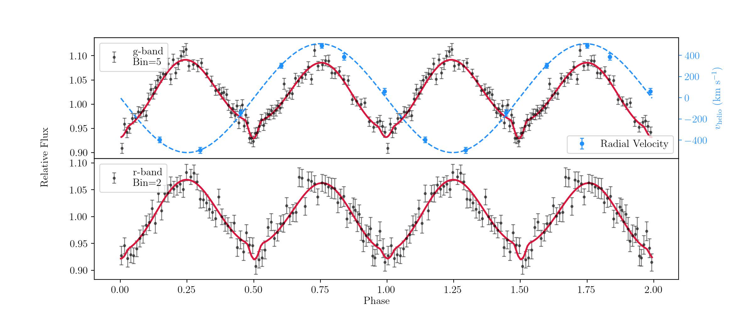
Figure 9: Top: McDonald 2.1-meter $g$-band (top; binned by 5) and $r$-band (bottom; binned by 2) light curves of ZTF J2049$+$3351. We overplot our radial velocity measurements as blue data points in the top panel.

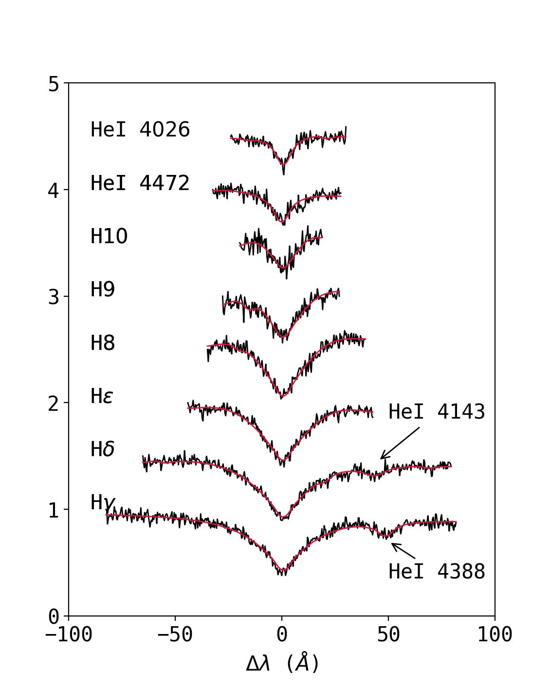
Figure 10: Best fitting spectroscopic model to the optical spectroscopy of J2049$+$3351, including rotational broadening.

To fit the co-added spectrum of J2049$+$3351, we use spectral models which were constructed using a hybrid LTE/NLTE approach described in detail in Przybilla et al. (2011) and Irrgang et al. (2021). The grid of spectral models covers a typical range of hot subdwarf $T_{\rm eff}$, and $\log{g}$, up to modest helium abundances (Heber, 2023; Irrgang et al., 2021, 2022). Our best-fitting parameters, with their bootstrapped uncertainties, are $T_{\rm eff}=17{\rm,}500\pm 500~{}{\rm K}$, $\log{g}=5.85\pm 0.05$, $\log{\frac{He}{H}}=-0.24\pm 0.07$, and $v_{\rm rot}=260\pm 60~{}{\rm km~{}s^{-1}}$. Best-fitting solutions without rotational broadening fail to reproduce the observed broad Helium absorption lines. We present the best-fitting model atmosphere over-plotted on our optical spectrum in Figure 10.

We obtained $218~{}{\rm min}$ of $g$-band and $108~{}{\rm min}$ of $r$-band high-speed photometry using the McDonald 2.1-meter telescope. We performed a simultaneous multi-band fit to our unbinned light curves using lcurve. We assign the time of primary conjunction using our radial velocity data and fit for the mass ratio, individual stellar radii, orbital inclination, and effective temperatures.

Our best-fitting model identifies primary and secondary eclipses in the data. However, J2049$+$3351 is faint (${\rm Gaia}~{}G=18.7~{}{\rm mag}$), and our 2.1-meter McDonald light curves are noisy. While the eclipses are not seen in our $r$-band light curve due to the high noise level, a relatively clean secondary-eclipse feature can be seen in the binned $g$-band light curve data and a noisy primary-eclipse feature may be visible in our unbinned $g$-band data. We present our binned and phase-folded McDonald 2.1-meter $g$- and $r$-band light curves in Figure 9 with the most-probable light curve model over-plotted as a red line and radial velocity curve over-plotted in blue.

Our best-fitting model to the McDonald 2.1-meter light curves finds mass ratio $q=\frac{M_{1}}{M_{2}}=0.39\pm 0.2$, inclination $i=74\pm 3^{\circ}$, $T_{\rm eff,1}=23{\rm,}200^{+4900}_{-4300}~{}{\rm K}$,$T_{\rm eff,2}=35{\rm,}400^{+9700}_{-8600}~{}{\rm K}$, $r_{1}=\frac{R_{1}}{a}=0.31\pm 0.05$, and $r_{2}=\frac{R_{2}}{a}=0.06^{+0.03}_{-0.02}$. We summarize these values in Table 3.

Because J2049$+$3351 is faint, large aperture high-speed photometry will be required to obtain sufficient signal-to-noise to confirm the presence of eclipses. These future observations will be used to place precise constraints on the binary parameters and determine the evolutionary history of J2049$+$3351.

J2102$-$4145

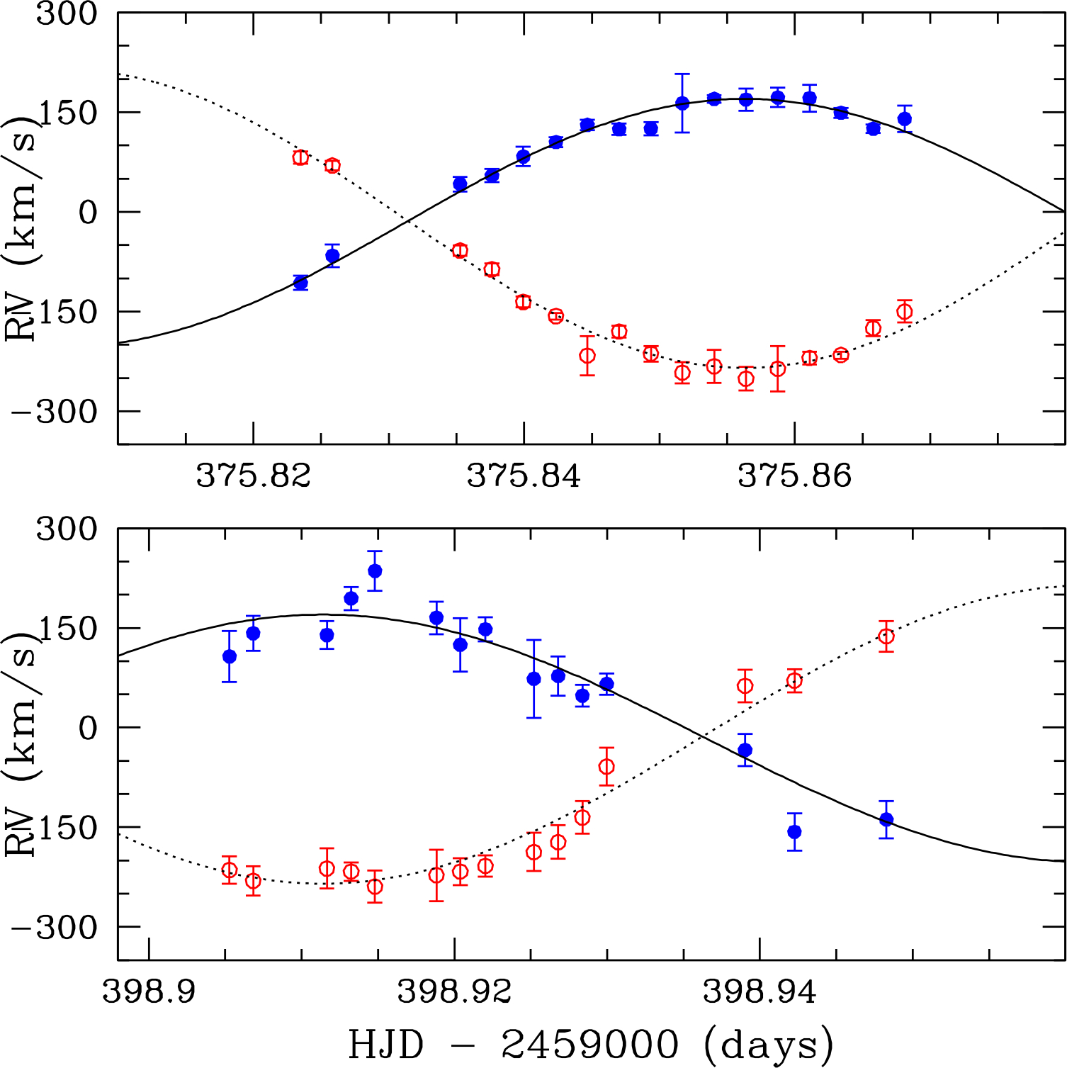
Figure 11: Orbital solutions for each component of the double-lined binary J2102$-$4145. Top: Magellan 6.5-meter telescope data. Bottom: Gemini South 8.1-meter telescope data. The blue/red points represent the radial velocity measurements for the primary/secondary star.

J210220.456$-$414501.736 (J2102$-$4145; Gaia DR3 6581249825853801984) is a relatively bright (Gaia ${\rm G}=15.7~{}{\rm mag}$) and nearby ($d_{\pi}=165\pm 1~{}{\rm pc}$) eclipsing low mass white dwarf binary. Our 6.5-meter Magellan spectroscopic follow-up observations reveal two nearly-equal depth absorption components, most easily seen in ${\rm H}\alpha$. Thus J2102$-$4145 is now the eighth confirmed double-lined, double-degenerate, eclipsing white dwarf binary published after CSS41177 (J1005$+$2249; Bours et al., 2014), ZTF J1539$+$5027 (Burdge et al., 2019), ZTF J1901+5309 Coughlin et al. (2020), and ZTF J0538$+$1953, ZTF J0722$-$1839, ZTF J1749$+$0924, and ZTF J2029$+$1534 (Burdge et al., 2020).

Because the individual absorption components are roughly equal-depth, obtaining a precise orbital period and individual velocity semi-amplitudes leads to significant period aliases when combining data over multiple nights. Our 55 radial velocity measurements for J2102$-$4145 provide orbital period constraints with strong period aliases between $P_{\rm RV}=2-3~{}{\rm h}$.

Fortunately, the TESS 2-minute cadence data archive provides a light curve for J2102$-$4145 (TIC 115013365). Our BLS algorithm identifies periodic eclipses in the TESS light curve with period $P_{\rm BLS}=1.2~{}{\rm h}$, with its phase-folded light curve showing a shallow primary eclipse heavily diluted by a bright (Gaia ${\rm G}=11.2~{}{\rm mag}$) field star roughly $30\arcsec$ away. Figure 3 (lower-left) shows the phase-folded TESS 2-minute cadence light curve and its BLS periodogram for J2102$-$4145.

Given that this is a double-lined spectroscopic binary with nearly-equal depth absorption components, our BLS algorithm will confuse the nearly-equal depth primary and secondary eclipses at the true orbital period with one primary eclipse occurring twice as often. Our BLS algorithm has identified the half-period; the true orbital period of J2102$-$4145 is therefore $P=2.4~{}{\rm h}$, in agreement with the constraints from our radial velocity analysis.

Using the TESS period, we were able to constrain the orbital solutions for both stars in the binary. Figure 11 displays our best-fitting orbital solution for each star, using data from Magellan and Gemini South. We find $P_{\rm RV}=144.3^{+0.4}_{-0.3}~{}{\rm min}$, $K_{1}=227\pm 8~{}{\rm km~{}s^{-1}}$, $\gamma_{1}=-8^{+7}_{-6}~{}{\rm km~{}s^{-1}}$, $K_{2}=186\pm 8~{}{\rm km~{}s^{-1}}$, and $\gamma_{2}=-19^{+6}_{-7}~{}{\rm km~{}s^{-1}}$, corresponding to binary mass ratio $q=0.82\pm 0.05$.

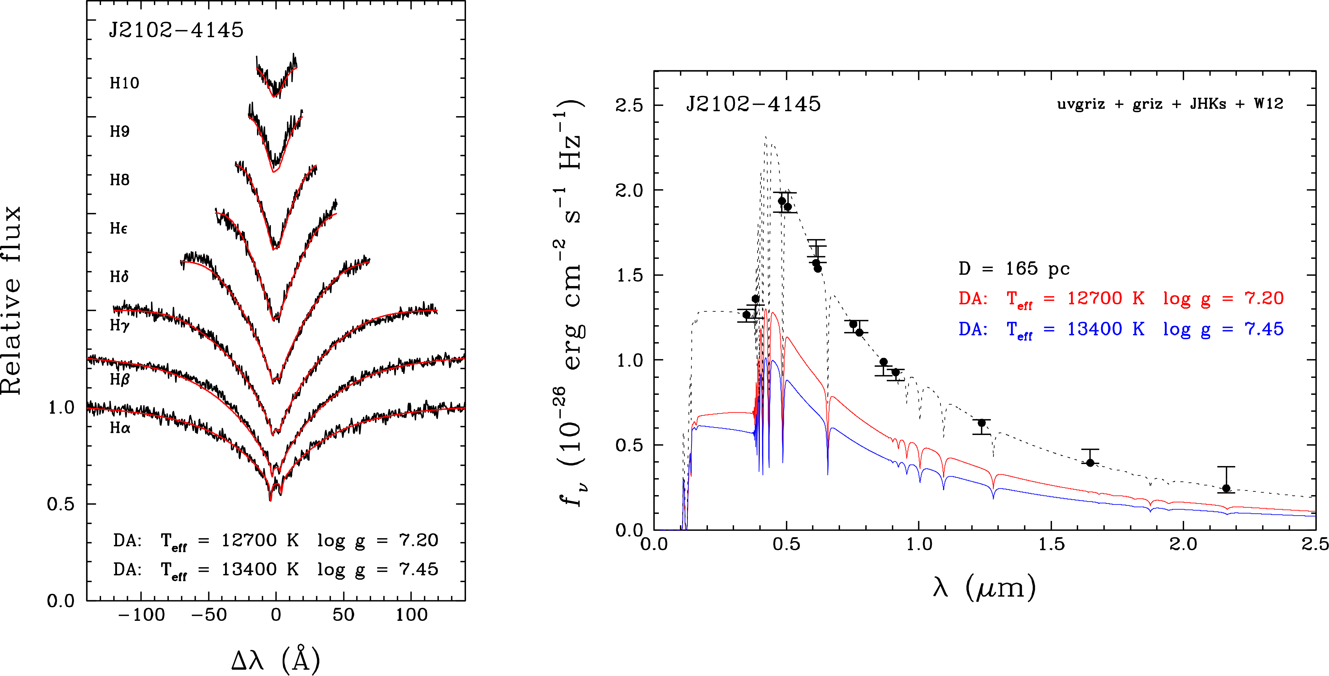
Figure 12: Best simultaneous model-atmosphere fit to the spectrum (left) and SED (right) of J2102$-$4145 including contributions from two DA white dwarfs. In the left panel, the observed and predicted Balmer lines are shown as black and red lines, respectively. In the right panel, the observed and predicted average fluxes are displayed as error bars and filled circles, respectively; for reference, the red and blue lines show the individual contributions of the components to the total monochromatic model flux, which is displayed as a black dotted line

Finally, we performed simultaneous model atmosphere fits to the SED and median-combined spectrum of J2102$-$4145, including the contributions of both components. To avoid significant smearing, our median combined spectrum used four consecutive spectra covering 9% of the orbit, approaching maximum separation. Our fits also made use of the Gaia DR3 parallax measurement and the mass ratio constraint provided by the orbital solution, thanks to which we were able to obtain a unique solution, shown in Figure 12.

Our best-fitting solution suggests that J2102$-$4145 contains two similar DA white dwarfs with atmospheric parameters $T_{\rm eff,1}=12{\rm,}700\pm 500~{}{\rm K}$, $\log{g}_{1}=7.20\pm 0.05$, $T_{\rm eff,2}=13{\rm,}400\pm 500~{}{\rm K}$, and $\log{g}_{2}=7.45\pm 0.05$, corresponding to masses $M_{1}=0.32~{}{\rm M_{\odot}}$ and $M_{2}=0.39~{}{\rm M_{\odot}}$ based on the He-core white dwarf tracks of Althaus et al. (2013), in agreement to within $2\sigma$ of the expected values based on the difference in systemic velocities measured from our radial velocity solution.

High-speed light curve follow-up of J2102$-$4145 will allow for a rare opportunity to directly measure the radii of the individual stars in the binary, independent of model estimates.

J2303$-$2615

We obtained 34 radial velocity measurements of J230323.542$-$261459.917 (J2303$-$2614; Gaia DR3 2382531303846872448), resulting in a best-fitting circular orbit with parameters $P_{\rm RV}=2.8367\pm 0.0008~{}{\rm h}$, $K=302.9\pm 2.3~{}{\rm km~{}s^{-1}}$ and $\gamma=-17.1\pm 2.1~{}{\rm km~{}s^{-1}}$. J2303$-$2614 is a disk object with $[U,V,W]=[31.1\pm 1.2,-60.0\pm 1.4,18.8\pm 1.4]~{}{\rm km~{}s^{-1}}$.

We fit the median-combined zero-velocity spectrum with pure-hydrogen atmosphere models and obtained best-fitting atmospheric parameters $T_{\rm eff}=11{\rm,}280\pm 170~{}{\rm K}$ and $\log{g}=5.43\pm 0.05$, corresponding to a white dwarf with mass $M_{1}=0.18\pm 0.01~{}{\rm M_{\odot}}$.

Our Lomb-Scargle periodogram identified strong periodic photometric variability in the TESS 2-minute cadence data of J2303$-$2614 (TIC 12970429) at frequency $f_{\rm TESS}=16.9392~{}{\rm cycles~{}d^{-1}}$ ($P=1.417~{}{\rm h}$), in good agreement with half the orbital period seen in our radial velocity follow-up, suggesting that J2303$-$2614 is another tidally distorted white dwarf in a compact binary. Figure 3 (lower-right) shows the phase-folded TESS 2-minute cadence light curve and its Lomb Scargle power spectrum. We provide a zoomed-inset plot showing a small, but significant, peak at the true orbital period of this system.

7 Discussion

7.1 Detectable LISA Binaries

General relativity predicts that the orbits of compact binaries decay due to the emission of gravitational waves. Binaries with orbital periods $P\lesssim 6~{}{\rm h}$ will merge within a Hubble time. The shortest period white dwarf binaries, with periods $P\lesssim 1~{}{\rm h}$, will be the dominant source of gravitational wave signal for the Laser Interferometer Space Antenna (LISA; Amaro-Seoane et al., 2017) mission, creating an incoherent noise floor in the LISA sensitivity range at mHz frequencies (Nelemans et al., 2001; Korol et al., 2017; Li et al., 2020; Amaro-Seoane et al., 2022).

Over 40 compact binaries have been characterized through their electromagnetic radiation and will be individually resolved by LISA, many of which will act as verification binaries for the LISA mission data calibration (see Finch et al., 2022; Kupfer et al., 2023, and references therein). These individually resolvable gravitational wave binaries will provide a multi-messenger approach to studying compact binary evolution through their electromagnetic and gravitational wave emission. We find that two of our 28 new binaries will be detected by LISA within a 4-year mission.

Our single star spectroscopic fits to J1506$-$1125 suggests that it contains an $M_{1}=0.43\pm 0.02~{}{\rm M_{\odot}}$ white dwarf in a $P=0.7757\pm 0.0094~{}{\rm h}$ binary with an $M_{2}>0.18\pm 0.01~{}{\rm M_{\odot}}$ companion at a distance of $d_{\pi}=413\pm 18~{}{\rm pc}$. We used the NASA LISA Detectability Calculator to estimate its expected LISA signal-to-noise ratio over 4-years of observation to be ${\rm SNR}=1.9$ assuming $i=90^{\circ}$, or ${\rm SNR}=3.7$ assuming $i=60^{\circ}$. However, our single-component fits to the SED of J1506$-$1125 suggests significant contribution to the total system light from an unseen companion. Our simultaneous multi-component fits to the available SED and optical spectroscopy of J1506$-$1125 (discussed in Section 6) suggest a large range of probable stellar parameters for each component. Over this range, we find signal to noise ratios between $3.9-4.7$ assuming $i=90^{\circ}$, or $6.1-7.3$ assuming $i=60^{\circ}$.

J152601.115$-$271156.660 (J1526$-$2711; Gaia DR3 6213619999912198144) is a $P=0.67\pm 0.01~{}{\rm h}$ binary containing an $M_{1}=0.37\pm 0.02~{}{\rm M_{\odot}}$ primary with an $M_{2}>0.40\pm 0.02~{}{\rm M_{\odot}}$ companion at a distance $d_{\pi}=623\pm 68~{}{\rm pc}$. J1526$-$2711 is a detectable LISA binary with 4-year signal-to-noise ${\rm SNR}=3.3$ assuming $i=90^{\circ}$, or ${\rm SNR}=6.4$ assuming $i=60^{\circ}$.

We find no photometric variability for either of these binaries in the public ZTF and TESS data archives. LISA detections will provide precise constraints to their orbital inclinations and chip masses, which will be used to directly constrain individual component masses, leading to estimates on the eventual merger outcomes.

Figure 13 displays the LISA 4-year sensitivity curve for the ELM Survey binaries (black) with the 28 new binaries presented here (blue). We calculated the gravitational wave strain for each of our new binaries using Equation 2, assuming $i=90^{\circ}$ if orbital inclination was not known through photometric constraints.

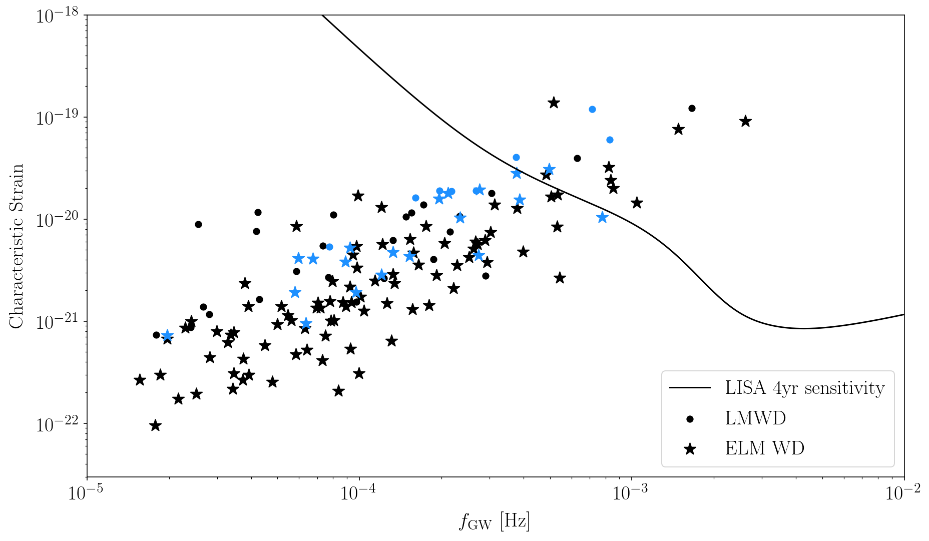
Figure 13: Four-year LISA sensitivity plot including the white dwarf binaries identified as part of the ELM Survey (black) and the 28 new white dwarf binaries from this work (blue). ELM white dwarfs ($M\leq 0.305~{}{\rm M_{\odot}}$) are marked as star symbols while low-mass white dwarfs are marked as circles.

7.2 Comparison with other surveys

Pelisoli & Vos (2019) created a catalog of 5672 ELM white dwarf candidates based on Gaia DR2 astrometry with extensive target cuts to remove contamination. We cross-matched our 28 new binaries with the Gaia DR2 ELM white dwarf candidate catalog of Pelisoli & Vos (2019) and find thirteen matches, which we mark in Tables 1 and 2. Many of the remaining binaries not reported as ELM white dwarf candidates in Pelisoli & Vos (2019) were excluded in their color cuts used to remove cataclysmic variables and WD+M binary contaminants.

Wang et al. (2022) used the LAMOST DR8 low resolution spectroscopy to further refine the candidate list of Pelisoli & Vos (2019) and identified 21 high probability ELM white dwarfs based on spectroscopic fits to the low resolution LAMOST data, including two of the new binaries we present in this work. Wang et al. (2022) identified J0215$+$0155 with atmospheric parameters $T_{\rm eff}=10{\rm,}540\pm 40~{}{\rm K}$ and $\log{g}=5.06\pm 0.07$, significantly lower than the values we find for our combined spectrum. Additionally, the authors identify significant radial velocity variability in two spectra of J1129$+$4715, with $T_{\rm eff,1}=11{\rm,}670\pm 50~{}{\rm K}$, $\log{g_{1}}=5.31\pm 0.06$, and $v_{\rm rad,1}=-38.9\pm 3.0~{}{\rm km~{}s^{-1}}$ and $T_{\rm eff,2}=11{\rm,}150\pm 90~{}{\rm K}$, $\log{g_{2}}=5.06\pm 0.02$, and $v_{\rm rad,2}=94.9\pm 5.4~{}{\rm km~{}s^{-1}}$, the first of which is in excellent agreement with the atmospheric parameter estimates from the fits presented in this work.

7.3 Conclusions

This work has identified 28 new low mass white dwarf binaries, bringing the total number of ELM Survey binaries to 148, with 41 located in the southern sky. Interestingly, this work identifies only three halo binaries among our 28 new binaries ($\approx 11\%$). Previous ELM Survey results suggest a significant contribution from halo objects of $\approx 30-40\%$ (Gianninas et al., 2015; Brown et al., 2022), likely due to the early ELM Survey target selection being based on photometry from SDSS, which observed at high Galactic latitudes. Additionally, our low fraction of new Halo objects is likely affected by our Gaia-based selection, and in-progress object follow-up, favoring nearby objects with reliable parallax measurements, rather than more distant halo objects.

Large-scale time-domain surveys are an excellent tool for the discovery of photometrically variable systems. Burdge et al. (2020) identified 15 ultra-compact ($P<1~{}{\rm h}$) binaries which show photometric variability in the ZTF data archive. We used the ZTF and TESS data archives to identify photometric variability in seven of our new binaries, including three short period eclipsing binaries. These short-period eclipsing binaries are especially important for determining precise physical parameters of both stars in the binary, which are valuable for binary population studies. Similar upcoming large-scale time-domain surveys, such as BlackGEM (Bloemen et al., 2015) and the Vera C. Rubin Observatory’s Legacy Survey of Space and Time (LSST) program (Ivezić et al., 2019) will enable efficient identification and characterization of white dwarf binaries in the southern sky, which will quickly expand the known population of ELM white dwarf binaries and allow for a more detailed population study of all-sky ELM white dwarf binaries.

8 Appendix

Object	HJD	$v_{\rm r}$
	($-2450000~{}{\rm days}$)	(${\rm km~{}s^{-1}}$)
J0135$+$2359	9192.787768	$133.7\pm 7.0$
J0135$+$2359	9548.737532	$7.4\pm 10.6$
J0135$+$2359	9548.786808	$-17.7\pm 10.0$
J0135$+$2359	9548.834528	$-72.6\pm 9.5$
J0135$+$2359	9549.572076	$110.4\pm 16.5$
J0135$+$2359	9549.712261	$117.2\pm 13.1$
J0135$+$2359	9549.776407	$139.2\pm 9.6$
J0135$+$2359	9549.821702	$74.6\pm 12.7$
J0135$+$2359	9549.827105	$98.2\pm 13.5$
J0135$+$2359	9549.831960	$84.5\pm 14.8$
J0135$+$2359	9549.837437	$103.3\pm 14.2$
J0135$+$2359	9550.562962	$-14.0\pm 8.6$
J0135$+$2359	9550.782942	$113.2\pm 8.5$
J0135$+$2359	9551.560708	$-192.1\pm 10.9$
J0135$+$2359	9551.568185	$-200.6\pm 13.3$
J0135$+$2359	9551.574674	$-171.2\pm 8.7$
J0135$+$2359	9551.664734	$-107.1\pm 8.3$
J0135$+$2359	9551.767718	$-1.4\pm 9.1$
J0155$-$4148	8778.528269	$120.9\pm 4.5$
J0155$-$4148	8778.747847	$93.1\pm 5.5$
J0155$-$4148	8780.584034	$107.9\pm 9.8$
J0155$-$4148	8780.591087	$62.2\pm 8.2$
J0155$-$4148	8781.538707	$199.1\pm 2.5$
J0155$-$4148	8781.631074	$103.9\pm 2.0$
$\cdots$	$\cdots$	$\cdots$

Table 4: Radial velocity measurements for the 28 new binaries identified in this work. This table has been truncated. The complete version of this table is available in the supplemental data files.

Table 5: Atmospheric parameters (assuming pure-hydrogen atmospheres) for objects observed as part of our follow-up campaign with $\log{g}>5.0$. Objects which show periodic photometric variability in ZTF DR16 or TESS high-cadence data, and objects which were classified as ELM white dwarf candidates in Pelisoli & Vos (2019), are marked. Optical spectroscopy for each object presented in this table is available in a public Zenodo archive (Kosakowski et al., 2023).

source_id	R.A.	Decl.	$T_{\rm eff}$	$\log{g}$	Gaia $G$	Gaia ($BP-RP$)	Gaia Parallax
(Gaia DR3)	(2016.0)	(2016.0)	(K)	(${\rm cm~{}s^{-2}}$)	(mag)	(mag)	(mas)
2882002220454588672	00:03:06.730	$+$40:39:27.119	$19250\pm 470$	$8.00\pm 0.07$	$18.49$	$0.01\pm 0.01$	$1.71\pm 0.32$
2739093475807603584	00:03:19.659	$+$02:26:23.089	$21790\pm 1190$	$8.35\pm 0.18$	$16.39$	$-0.098\pm 0.005$	$6.32\pm 0.07$
279838611350760499212	00:03:33.944	$+$20:16:26.238	$17760\pm 540$	$7.72\pm 0.10$	$18.95$	$0.07\pm 0.02$	$2.25\pm 0.25$
2874194833198918400	00:03:42.161	$+$32:44:15.731	$16410\pm 440$	$7.79\pm 0.08$	$18.22$	$0.22\pm 0.01$	$3.30\pm 0.14$
2448821478361661696	00:05:04.760	$-$01:27:08.384	$31340\pm 1380$	$7.68\pm 0.31$	$16.63$	$-0.33\pm 0.01$	$3.66\pm 0.07$
42025138730098009612	00:07:09.001	$+$53:49:47.474	$32980\pm 1930$	$6.15\pm 0.35$	$16.17$	$0.071\pm 0.004$	$0.96\pm 0.04$
285982610600930521612	00:12:32.540	$+$27:47:09.460	$25990\pm 860$	$7.37\pm 0.13$	$16.98$	$-0.31\pm 0.01$	$2.89\pm 0.09$
276840988748171827212	00:12:45.662	$+$14:39:56.678	$14580\pm 410$	$7.38\pm 0.08$	$18.19$	$0.07\pm 0.01$	$2.78\pm 0.18$
280021054689570368012	00:15:48.404	$+$21:27:46.332	$32970\pm 1020$	$7.35\pm 0.21$	$17.51$	$-0.30\pm 0.01$	$1.85\pm 0.10$
2876543282660374784	00:17:44.512	$+$35:58:26.087	$18410\pm 430$	$7.95\pm 0.07$	$18.85$	$0.03\pm 0.02$	$1.88\pm 0.23$
28636211348162305281012	00:18:11.384	$+$33:11:08.826	$30630\pm 590$	$7.44\pm 0.09$	$18.04$	$-0.29\pm 0.01$	$1.28\pm 0.14$
2855799415254881408	00:20:22.382	$+$26:40:10.956	$11820\pm 220$	$8.02\pm 0.13$	$16.11$	$-0.111\pm 0.005$	$10.51\pm 0.05$
38056094167742476811	00:33:52.632	$+$38:55:29.608	$34130\pm 700$	$7.30\pm 0.13$	$18.34$	$-0.19\pm 0.02$	$1.19\pm 0.17$
4907063048361514496	00:40:00.768	$-$58:40:31.721	$38240\pm 750$	$7.28\pm 0.09$	$17.58$	$-0.24\pm 0.02$	$1.14\pm 0.08$
2542961560852591744	00:40:22.906	$-$00:21:30.172	$16470\pm 510$	$8.16\pm 0.09$	$14.85$	$0.046\pm 0.004$	$18.24\pm 0.03$
2550740120286280576	00:45:36.928	$+$02:40:14.491	$15140\pm 480$	$5.03\pm 0.10$	$18.85$	$0.31\pm 0.02$	$0.93\pm 0.27$
280908501877659852812	00:49:11.206	$+$28:16:02.255	$27850\pm 2870$	$5.68\pm 0.42$	$16.56$	$-0.32\pm 0.01$	$0.59\pm 0.07$
377520826387065856	00:52:04.391	$+$45:05:33.799	$11730\pm 180$	$8.21\pm 0.11$	$16.01$	$-0.039\pm 0.004$	$13.28\pm 0.04$
277683651453233830412	00:52:44.411	$+$13:16:35.972	$36500\pm 1560$	$7.33\pm 0.28$	$17.94$	$-0.32\pm 0.01$	$1.11\pm 0.13$
37444799632898470412	01:01:10.344	$+$41:06:04.921	$21740\pm 510$	$7.36\pm 0.07$	$18.41$	$-0.24\pm 0.02$	$1.68\pm 0.17$
2785461702216001152	01:07:25.996	$+$19:09:32.166	$21940\pm 1260$	$7.56\pm 0.19$	$15.64$	$-0.276\pm 0.005$	$5.93\pm 0.05$
257974269440644006412	01:09:29.505	$+$09:19:51.845	$32350\pm 1030$	$7.81\pm 0.23$	$17.37$	$-0.36\pm 0.01$	$1.53\pm 0.11$
2534408386884529920	01:12:58.398	$-$00:59:52.519	$19380\pm 610$	$7.58\pm 0.10$	$18.84$	$-0.27\pm 0.03$	$1.09\pm 0.25$
373358998783703808	01:16:00.832	$+$42:49:38.323	$12970\pm 200$	$5.06\pm 0.05$	$18.71$	$-0.00\pm 0.02$	$0.57\pm 0.18$
32004014519252326412	01:16:20.951	$+$33:41:16.094	$13880\pm 240$	$7.42\pm 0.05$	$18.16$	$-0.06\pm 0.01$	$2.16\pm 0.16$
248281040643248051211	01:16:51.573	$-$04:40:47.107	$45500\pm 870$	$7.58\pm 0.10$	$18.34$	$-0.25\pm 0.02$	$1.02\pm 0.18$
2471069512033475712	01:21:49.346	$-$10:08:00.751	$17340\pm 490$	$7.95\pm 0.09$	$17.31$	$0.07\pm 0.01$	$8.58\pm 0.10$
256335372197558246412	01:25:43.673	$+$04:55:14.686	$18120\pm 450$	$7.60\pm 0.08$	$18.15$	$0.19\pm 0.01$	$4.07\pm 0.19$
5316176902616983041011	01:33:38.050	$+$68:03:32.789	$34860\pm 1030$	$7.58\pm 0.21$	$16.72$	$0.21\pm 0.01$	$2.60\pm 0.05$
296853330452496000	01:34:46.322	$+$28:26:16.202	$12300\pm 330$	$7.89\pm 0.11$	$16.91$	$0.02\pm 0.01$	$5.68\pm 0.07$
315437516503244928	01:35:01.880	$+$31:17:10.212	$18700\pm 500$	$7.93\pm 0.09$	$19.07$	$-0.17\pm 0.02$	$2.33\pm 0.32$
322765211746880384	01:38:52.560	$+$38:34:01.819	$34230\pm 680$	$7.83\pm 0.12$	$18.46$	$-0.36\pm 0.02$	$1.29\pm 0.18$
347329027362621056	01:40:12.938	$+$41:29:27.074	$25380\pm 550$	$7.76\pm 0.08$	$18.36$	$-0.28\pm 0.01$	$2.13\pm 0.20$
319243613441880320	01:43:20.592	$+$36:28:42.978	$36240\pm 1140$	$8.27\pm 0.21$	$17.23$	$-0.37\pm 0.01$	$2.39\pm 0.09$
513928736021067814412	01:48:11.827	$-$19:48:14.188	$15090\pm 240$	$7.74\pm 0.05$	$18.82$	$0.03\pm 0.01$	$1.56\pm 0.19$
92185017673400960	01:52:27.290	$+$18:20:14.374	$34580\pm 990$	$7.81\pm 0.20$	$17.43$	$-0.19\pm 0.01$	$1.99\pm 0.12$
5134761186235143424	01:55:58.754	$-$22:38:22.520	$23910\pm 610$	$7.58\pm 0.09$	$17.64$	$-0.32\pm 0.01$	$2.30\pm 0.10$
246676694693976128011	01:58:41.010	$-$06:28:41.650	$22740\pm 550$	$7.74\pm 0.08$	$16.91$	$0.12\pm 0.01$	$3.55\pm 0.08$
496886649387926976012	01:59:48.100	$-$35:16:51.229	$21850\pm 720$	$7.52\pm 0.10$	$17.92$	$-0.24\pm 0.01$	$1.97\pm 0.10$
104648944047154432	02:08:47.713	$+$25:14:08.045	$20880\pm 440$	$8.05\pm 0.06$	$13.23$	$-0.208\pm 0.004$	$25.59\pm 0.03$
5136945744040876928	02:09:30.476	$-$20:19:33.535	$27690\pm 500$	$7.53\pm 0.07$	$18.30$	$-0.29\pm 0.02$	$1.68\pm 0.17$
4715247167518325376	02:10:35.380	$-$57:49:57.976	$26780\pm 460$	$7.58\pm 0.06$	$17.66$	$-0.33\pm 0.01$	$2.29\pm 0.07$
331359166428843904	02:13:28.349	$+$37:16:49.814	$24300\pm 2040$	$6.79\pm 0.28$	$17.80$	$-0.29\pm 0.01$	$1.92\pm 0.14$
4744277057630500352	02:13:54.959	$-$53:04:53.962	$26430\pm 400$	$7.42\pm 0.05$	$17.29$	$-0.33\pm 0.01$	$2.34\pm 0.07$
2493466422156808576	02:23:17.915	$-$02:42:52.495	$28000\pm 670$	$7.36\pm 0.10$	$18.11$	$-0.05\pm 0.02$	$1.36\pm 0.16$
513132765623527308812	02:27:41.362	$-$18:59:25.656	$17550\pm 2300$	$7.81\pm 0.45$	$15.98$	$-0.120\pm 0.004$	$6.45\pm 0.04$
76220791737582720	02:28:45.867	$+$15:42:02.599	$37170\pm 1120$	$7.21\pm 0.19$	$18.26$	$-0.07\pm 0.02$	$1.20\pm 0.19$
131694078232129792	02:30:14.426	$+$30:56:11.627	$24620\pm 550$	$7.30\pm 0.07$	$18.55$	$-0.08\pm 0.02$	$1.63\pm 0.19$
5130174745278506112	02:33:01.035	$-$20:25:59.635	$16810\pm 590$	$7.55\pm 0.12$	$19.63$	$-0.14\pm 0.04$	$1.88\pm 0.32$
18117653818752512	02:35:47.678	$+$05:35:24.083	$24640\pm 760$	$7.31\pm 0.11$	$15.79$	$-0.36\pm 0.01$	$5.22\pm 0.07$
4741227287252719872	02:38:43.420	$-$55:01:27.966	$18700\pm 410$	$7.41\pm 0.07$	$17.43$	$-0.22\pm 0.01$	$2.22\pm 0.06$
2502595323604529408	02:40:09.470	$+$01:51:49.248	$17710\pm 300$	$7.41\pm 0.05$	$18.44$	$-0.19\pm 0.02$	$1.92\pm 0.18$
4952731126381731328	02:45:09.857	$-$38:05:40.247	$14240\pm 280$	$7.84\pm 0.05$	$18.06$	$-0.09\pm 0.01$	$2.42\pm 0.10$
6306661258129280	02:48:45.909	$+$05:39:21.758	$12410\pm 280$	$7.86\pm 0.09$	$19.04$	$0.13\pm 0.02$	$1.50\pm 0.38$
11570872105679014412	03:01:45.948	$+$26:55:44.879	$30780\pm 810$	$7.76\pm 0.16$	$18.55$	$-0.08\pm 0.02$	$1.43\pm 0.19$
5104166386135159936	03:06:39.346	$-$19:02:24.893	$35530\pm 650$	$8.20\pm 0.09$	$17.32$	$-0.08\pm 0.01$	$2.71\pm 0.08$
326267448768244044812	03:18:13.332	$-$01:07:11.806	$12450\pm 1480$	$7.52\pm 0.44$	$14.71$	$-0.062\pm 0.004$	$14.25\pm 0.03$
3260723782255411456	03:23:22.673	$-$03:54:20.808	$28440\pm 630$	$7.88\pm 0.10$	$18.50$	$-0.32\pm 0.03$	$2.22\pm 0.24$
23713356684752000012	03:38:47.068	$+$41:34:24.100	$23460\pm 430$	$5.82\pm 0.06$	$15.09$	$-0.061\pm 0.004$	$1.65\pm 0.03$
6988685314399449612	03:44:22.259	$+$25:14:53.293	$28280\pm 1340$	$6.45\pm 0.22$	$15.55$	$-0.006\pm 0.004$	$1.79\pm 0.04$
5113854281871286912	03:45:32.977	$-$14:04:58.102	$11140\pm 320$	$5.02\pm 0.10$	$18.64$	$0.18\pm 0.02$	$0.58\pm 0.18$
4858747758657659136	03:51:23.934	$-$34:45:50.306	$15450\pm 450$	$7.34\pm 0.09$	$18.14$	$-0.18\pm 0.01$	$2.54\pm 0.10$
4887600528615197184	03:52:10.364	$-$30:25:23.981	$28540\pm 890$	$7.40\pm 0.15$	$17.21$	$-0.21\pm 0.01$	$2.45\pm 0.07$
3251978198050225664	04:03:24.704	$-$03:28:51.614	$26600\pm 450$	$7.43\pm 0.06$	$16.68$	$-0.30\pm 0.01$	$3.32\pm 0.06$
484402306457895232012	04:04:44.429	$-$39:50:43.206	$35120\pm 780$	$7.54\pm 0.13$	$17.66$	$-0.27\pm 0.02$	$1.58\pm 0.07$
468172962069729536010	04:10:33.371	$-$58:52:03.482	$32040\pm 480$	$7.28\pm 0.06$	$17.57$	$-0.15\pm 0.02$	$1.52\pm 0.07$
4830937162517646592	04:13:45.134	$-$47:37:25.612	$18500\pm 360$	$7.84\pm 0.06$	$16.54$	$-0.14\pm 0.01$	$5.33\pm 0.04$
166283580171410816	04:20:32.033	$+$31:09:08.701	$34450\pm 760$	$7.25\pm 0.13$	$18.70$	$0.05\pm 0.02$	$1.44\pm 0.20$
320435278317351372811	04:31:03.755	$-$04:17:02.555	$36010\pm 700$	$7.59\pm 0.11$	$17.92$	$-0.32\pm 0.02$	$0.98\pm 0.14$
318525460979800332812	04:34:38.049	$-$10:14:07.246	$17460\pm 2920$	$8.03\pm 0.63$	$16.53$	$0.004\pm 0.004$	$6.68\pm 0.05$
3229440649222191616	04:36:59.954	$-$01:15:53.903	$31190\pm 550$	$8.05\pm 0.08$	$17.91$	$-0.30\pm 0.01$	$2.68\pm 0.12$
4814354976686021888	04:47:19.788	$-$44:44:10.622	$20900\pm 530$	$7.69\pm 0.08$	$16.93$	$-0.27\pm 0.01$	$3.71\pm 0.05$
322535919334081228812	04:59:20.296	$-$02:28:06.650	$32550\pm 1450$	$6.09\pm 0.29$	$15.05$	$-0.398\pm 0.004$	$1.11\pm 0.04$
2979874526445650560	05:01:59.217	$-$17:09:56.642	$26160\pm 410$	$7.48\pm 0.05$	$18.42$	$-0.12\pm 0.01$	$1.30\pm 0.14$
3211273483020379136	05:07:42.284	$-$05:50:52.811	$31150\pm 540$	$7.82\pm 0.08$	$18.31$	$-0.35\pm 0.01$	$1.50\pm 0.17$
2971802603565750016	05:31:27.482	$-$15:56:26.520	$29490\pm 470$	$7.95\pm 0.06$	$16.55$	$-0.325\pm 0.005$	$3.97\pm 0.06$
482168329470173145612	05:32:25.215	$-$36:40:57.058	$24710\pm 640$	$7.30\pm 0.09$	$17.38$	$-0.30\pm 0.01$	$2.28\pm 0.06$
2965034525384116864	05:32:46.106	$-$21:03:40.381	$27600\pm 460$	$7.53\pm 0.06$	$17.72$	$-0.22\pm 0.01$	$1.82\pm 0.09$
3402486457838073728	05:38:02.721	$+$19:53:02.893	$37120\pm 1080$	$7.33\pm 0.16$	$18.80$	$0.02\pm 0.02$	$0.96\pm 0.29$
48057007550270348812	05:39:59.130	$+$66:30:43.434	$39310\pm 2520$	$7.13\pm 0.27$	$16.43$	$-0.228\pm 0.005$	$1.61\pm 0.05$
19172771805138931212	05:47:06.231	$+$40:08:22.524	$28290\pm 4040$	$5.33\pm 0.53$	$15.75$	$-0.061\pm 0.004$	$1.02\pm 0.05$
480529795581120038412	05:47:14.337	$-$39:22:53.227	$31790\pm 520$	$7.59\pm 0.07$	$18.26$	$-0.17\pm 0.01$	$1.25\pm 0.11$
2904788774305591168	05:49:05.586	$-$27:51:03.064	$21370\pm 620$	$7.44\pm 0.09$	$19.18$	$-0.16\pm 0.02$	$1.34\pm 0.18$
312300486563891020812	06:09:30.047	$+$01:00:43.243	$35800\pm 2690$	$6.20\pm 0.45$	$16.36$	$-0.067\pm 0.005$	$0.71\pm 0.06$
1106926566694585984	06:19:13.539	$+$69:11:37.003	$36910\pm 750$	$7.98\pm 0.10$	$16.89$	$-0.092\pm 0.005$	$3.22\pm 0.06$
299974520982174617612	06:20:42.669	$-$13:07:30.864	$36350\pm 3360$	$6.15\pm 0.53$	$16.14$	$-0.170\pm 0.005$	$1.10\pm 0.05$
94342956559923212812	06:34:49.904	$+$38:03:51.977	$22560\pm 430$	$7.18\pm 0.06$	$17.13$	$-0.19\pm 0.01$	$2.31\pm 0.08$
96772241172553945612	06:38:40.371	$+$48:29:50.784	$30210\pm 5070$	$5.43\pm 0.82$	$16.15$	$-0.309\pm 0.005$	$0.68\pm 0.06$
114124891736817164812	06:43:34.284	$+$79:20:36.190	$16930\pm 530$	$7.91\pm 0.10$	$18.86$	$-0.18\pm 0.05$	$2.24\pm 0.16$
335121630364379609612	06:45:32.028	$+$11:40:03.173	$27350\pm 3840$	$5.30\pm 0.48$	$16.85$	$0.07\pm 0.01$	$0.67\pm 0.06$
335283598305328230412	06:47:34.863	$+$13:50:11.332	$31730\pm 1640$	$6.16\pm 0.33$	$16.80$	$-0.19\pm 0.01$	$0.55\pm 0.07$
110639021117786188812	06:47:46.546	$+$69:15:34.430	$32030\pm 680$	$7.27\pm 0.12$	$17.90$	$-0.46\pm 0.01$	$1.47\pm 0.11$
100049707093804249612	06:58:37.717	$+$57:12:35.755	$34520\pm 1960$	$5.25\pm 0.28$	$16.21$	$-0.367\pm 0.005$	$0.56\pm 0.06$
979204650309974016	07:00:04.137	$+$49:43:38.687	$35320\pm 1580$	$7.60\pm 0.33$	$17.43$	$-0.31\pm 0.01$	$2.44\pm 0.11$
990086409514581760	07:07:17.295	$+$58:01:36.512	$23590\pm 510$	$7.42\pm 0.07$	$16.92$	$-0.30\pm 0.01$	$3.31\pm 0.07$
549001587136783744012	07:07:30.007	$-$56:17:43.206	$32240\pm 480$	$7.14\pm 0.06$	$15.89$	$-0.343\pm 0.004$	$2.34\pm 0.03$
316116939097852659212	07:12:06.982	$+$13:23:49.200	$14790\pm 490$	$7.85\pm 0.08$	$18.83$	$-0.15\pm 0.02$	$2.00\pm 0.23$
110203147220522483211	07:14:52.278	$+$66:29:28.648	$22320\pm 760$	$7.47\pm 0.11$	$18.87$	$0.26\pm 0.01$	$1.39\pm 0.17$
989858913686629248	07:20:10.814	$+$57:30:54.979	$30920\pm 1030$	$7.58\pm 0.21$	$17.87$	$-0.34\pm 0.01$	$2.17\pm 0.13$
900688761191934208	07:30:30.416	$+$41:15:39.827	$29150\pm 800$	$7.96\pm 0.14$	$17.64$	$-0.40\pm 0.01$	$2.66\pm 0.12$
316916548621049548812	07:34:29.881	$+$16:48:22.968	$16540\pm 560$	$8.02\pm 0.10$	$19.02$	$0.04\pm 0.04$	$2.04\pm 0.30$
3165507445385638528	07:42:11.606	$+$14:53:17.970	$17080\pm 510$	$7.74\pm 0.09$	$19.02$	$-0.01\pm 0.03$	$2.32\pm 0.24$
67169949172539212812	07:45:44.371	$+$18:58:49.631	$15620\pm 400$	$7.69\pm 0.08$	$17.54$	$0.07\pm 0.01$	$3.93\pm 0.10$
66891212667020736012	08:02:42.951	$+$17:50:00.848	$21930\pm 1520$	$7.66\pm 0.23$	$16.27$	$-0.216\pm 0.005$	$4.23\pm 0.06$
306388573602335590412	08:06:50.022	$-$07:16:36.109	$13640\pm 550$	$6.46\pm 0.14$	$18.55$	$-0.07\pm 0.02$	$0.93\pm 0.18$
65322876153223321612	08:07:39.280	$+$13:21:11.434	$15560\pm 1910$	$7.44\pm 0.43$	$16.43$	$0.097\pm 0.004$	$8.71\pm 0.05$
309652594558180057611	08:11:26.652	$+$05:39:11.441	$26860\pm 720$	$7.87\pm 0.11$	$16.54$	$0.02\pm 0.01$	$4.57\pm 0.06$
307011505780551756812	08:18:41.061	$-$02:14:13.434	$33450\pm 1740$	$5.13\pm 0.33$	$16.49$	$-0.35\pm 0.01$	$0.50\pm 0.06$
309036142626473600012	08:20:00.642	$+$02:23:27.107	$14760\pm 370$	$7.53\pm 0.07$	$18.44$	$-0.01\pm 0.02$	$2.29\pm 0.19$
92858532969388083212	08:20:10.339	$+$45:43:01.704	$17360\pm 250$	$7.46\pm 0.04$	$18.21$	$-0.08\pm 0.01$	$2.38\pm 0.18$
3090457599171887104	08:21:01.664	$+$02:32:09.316	$23240\pm 950$	$7.54\pm 0.14$	$18.81$	$0.35\pm 0.02$	$1.40\pm 0.22$
112342363915470246412	08:21:42.669	$+$73:55:29.406	$35660\pm 1370$	$6.06\pm 0.24$	$14.43$	$-0.452\pm 0.004$	$1.75\pm 0.04$
70906471076786406412	08:23:59.152	$+$31:11:51.893	$19680\pm 390$	$7.57\pm 0.06$	$18.29$	$-0.20\pm 0.01$	$1.98\pm 0.18$
5196549827003398656	08:28:48.624	$-$80:19:35.026	$24480\pm 370$	$7.54\pm 0.05$	$15.33$	$-0.328\pm 0.004$	$7.14\pm 0.03$
707909910025230080	08:28:55.281	$+$29:21:00.310	$15560\pm 390$	$7.74\pm 0.07$	$18.85$	$-0.00\pm 0.03$	$1.95\pm 0.23$
307364156955251686412	08:36:01.849	$-$00:44:22.974	$26820\pm 480$	$6.02\pm 0.06$	$15.92$	$-0.349\pm 0.004$	$1.06\pm 0.06$
662771594747150976	08:36:12.031	$+$19:17:55.853	$33230\pm 2400$	$5.36\pm 0.48$	$15.69$	$-0.092\pm 0.005$	$0.53\pm 0.07$
66463117814753472012	08:36:19.698	$+$20:57:47.358	$30820\pm 1540$	$6.03\pm 0.29$	$16.31$	$-0.43\pm 0.01$	$0.54\pm 0.09$
307835304559705369612	08:40:14.857	$+$00:42:39.028	$33580\pm 1900$	$5.92\pm 0.37$	$16.47$	$-0.325\pm 0.005$	$0.59\pm 0.05$
582675157663938304	08:48:23.744	$+$05:08:44.930	$16100\pm 330$	$7.78\pm 0.07$	$17.42$	$-0.12\pm 0.01$	$2.59\pm 0.09$
60505207471517900812	08:54:08.733	$+$12:22:26.504	$15020\pm 280$	$7.50\pm 0.05$	$18.50$	$-0.02\pm 0.01$	$2.41\pm 0.20$
684882528766947456	08:57:45.557	$+$20:38:50.381	$11400\pm 310$	$5.04\pm 0.10$	$18.20$	$0.22\pm 0.01$	$0.90\pm 0.18$
718805520500404608	09:00:14.503	$+$37:57:49.241	$22340\pm 540$	$7.48\pm 0.08$	$19.15$	$-0.38\pm 0.03$	$0.95\pm 0.27$
61121507790691264012	09:03:00.839	$+$17:21:32.170	$11690\pm 210$	$7.83\pm 0.06$	$18.38$	$0.01\pm 0.01$	$2.50\pm 0.18$
1009623532844468480	09:08:46.276	$+$45:16:52.561	$11870\pm 330$	$7.87\pm 0.10$	$18.27$	$-0.09\pm 0.01$	$2.94\pm 0.16$
1009618997359086848	09:09:19.116	$+$45:10:51.697	$16700\pm 460$	$8.00\pm 0.08$	$19.04$	$-0.04\pm 0.02$	$2.14\pm 0.30$
638506468336791296	09:17:29.690	$+$21:43:33.452	$20540\pm 540$	$7.85\pm 0.08$	$18.85$	$-0.02\pm 0.02$	$1.51\pm 0.29$
38459452327563119361012	09:23:37.323	$+$03:53:09.208	$31520\pm 730$	$7.35\pm 0.14$	$17.53$	$-0.35\pm 0.01$	$1.61\pm 0.12$
817452604232788224	09:24:39.388	$+$42:36:33.415	$11260\pm 260$	$7.87\pm 0.08$	$18.79$	$-0.15\pm 0.02$	$1.41\pm 0.18$
568957963698962060812	09:25:09.586	$-$14:11:22.556	$26680\pm 3340$	$7.07\pm 0.48$	$15.39$	$-0.374\pm 0.004$	$4.07\pm 0.04$
1063375422215251456	09:36:36.353	$+$62:56:05.593	$15550\pm 580$	$7.54\pm 0.12$	$18.24$	$0.55\pm 0.01$	$2.54\pm 0.12$
79427658704353945612	09:37:08.551	$+$33:34:04.141	$24620\pm 830$	$7.33\pm 0.12$	$16.36$	$-0.323\pm 0.005$	$3.11\pm 0.08$
61682320997908147211	09:52:50.473	$+$15:53:04.013	$22810\pm 620$	$7.58\pm 0.09$	$18.31$	$0.42\pm 0.02$	$1.35\pm 0.20$
3879591353717543040	09:53:02.996	$+$10:32:20.094	$11610\pm 240$	$7.81\pm 0.07$	$18.79$	$-0.13\pm 0.02$	$1.73\pm 0.25$
1146182357322101120	10:07:52.208	$+$81:40:46.549	$19280\pm 740$	$7.66\pm 0.13$	$18.63$	$0.30\pm 0.01$	$1.41\pm 0.21$
375220059649383923212	10:24:32.206	$-$14:34:20.503	$9290\pm 150$	$8.20\pm 0.10$	$16.81$	$-0.13\pm 0.01$	$2.82\pm 0.09$
376787066441425011211	10:26:53.472	$-$10:13:30.194	$22150\pm 670$	$7.53\pm 0.09$	$18.35$	$-0.15\pm 0.03$	$1.65\pm 0.19$
54678518429593998081011	10:30:39.621	$-$27:54:38.876	$32020\pm 800$	$7.75\pm 0.16$	$18.31$	$-0.04\pm 0.02$	$1.31\pm 0.18$
1048058916002814080	10:33:50.070	$+$60:44:01.421	$19570\pm 530$	$7.50\pm 0.09$	$18.54$	$-0.24\pm 0.01$	$1.86\pm 0.14$
5468388683808323328	10:35:51.946	$-$26:43:01.996	$23340\pm 810$	$7.48\pm 0.12$	$18.92$	$-0.27\pm 0.02$	$1.37\pm 0.24$
1071978142925329280	10:36:05.668	$+$67:38:17.232	$9370\pm 160$	$8.37\pm 0.16$	$17.67$	$-0.26\pm 0.01$	$2.22\pm 0.08$
3754558774057309568	10:36:42.062	$-$11:47:42.065	$23940\pm 590$	$7.86\pm 0.09$	$19.56$	$-0.25\pm 0.04$	$1.26\pm 0.37$
377701087451158080012	10:51:15.599	$-$04:54:52.938	$21230\pm 610$	$7.39\pm 0.09$	$17.92$	$-0.21\pm 0.01$	$2.14\pm 0.16$
3801572246288990720	10:51:59.289	$-$02:48:05.868	$27700\pm 460$	$7.29\pm 0.06$	$17.49$	$-0.34\pm 0.01$	$1.26\pm 0.20$
386590446117630784012	10:52:13.140	$+$08:06:31.482	$14480\pm 660$	$7.50\pm 0.15$	$17.73$	$0.06\pm 0.01$	$3.31\pm 0.13$
3758426443647179008	11:06:21.270	$-$10:56:47.407	$15870\pm 420$	$7.70\pm 0.09$	$18.17$	$-0.11\pm 0.01$	$1.98\pm 0.16$
3803538104360099328	11:06:27.670	$-$01:05:14.698	$30280\pm 630$	$7.56\pm 0.11$	$16.47$	$0.06\pm 0.01$	$3.03\pm 0.08$
3783864852042143616	11:22:56.309	$-$06:45:05.792	$25160\pm 1180$	$7.25\pm 0.18$	$17.97$	$0.15\pm 0.01$	$1.77\pm 0.13$
381263209201839910412	11:24:21.658	$+$03:30:26.003	$20360\pm 500$	$7.65\pm 0.07$	$18.16$	$-0.23\pm 0.02$	$2.02\pm 0.16$
3796545519645331584	11:27:21.271	$-$02:08:37.464	$23520\pm 720$	$7.90\pm 0.10$	$16.39$	$-0.260\pm 0.005$	$5.39\pm 0.07$
348492200282207987212	11:35:24.140	$-$26:54:41.544	$18160\pm 350$	$7.52\pm 0.06$	$17.62$	$-0.12\pm 0.01$	$2.91\pm 0.11$
389586196544090368012	11:51:24.105	$+$03:41:47.263	$19950\pm 470$	$7.61\pm 0.07$	$18.13$	$-0.24\pm 0.01$	$2.14\pm 0.14$
389231985007695603212	11:53:16.969	$+$01:45:08.284	$15000\pm 620$	$7.46\pm 0.11$	$18.74$	$0.01\pm 0.01$	$2.15\pm 0.26$
4013124296427540096	12:08:34.821	$+$29:08:50.208	$15980\pm 430$	$7.82\pm 0.07$	$18.89$	$-0.19\pm 0.02$	$2.06\pm 0.30$
3501205731372521984	12:35:49.147	$-$23:28:06.280	$19410\pm 610$	$7.73\pm 0.11$	$18.98$	$-0.02\pm 0.02$	$1.43\pm 0.24$
6157479215371911040	12:38:33.842	$-$35:07:23.412	$16130\pm 320$	$7.45\pm 0.06$	$19.00$	$-0.09\pm 0.02$	$1.30\pm 0.22$
3676893915531705984	12:47:29.573	$-$05:39:23.036	$25440\pm 530$	$7.69\pm 0.07$	$18.44$	$-0.26\pm 0.02$	$1.31\pm 0.19$
352567155301334796812	12:51:41.084	$-$13:50:12.520	$15440\pm 390$	$7.54\pm 0.08$	$18.52$	$0.16\pm 0.02$	$2.62\pm 0.22$
362567467388503168012	12:59:29.143	$-$10:17:48.257	$16820\pm 410$	$7.58\pm 0.08$	$18.14$	$0.12\pm 0.01$	$2.90\pm 0.16$
6193688224923108480	13:13:23.141	$-$25:03:08.309	$28540\pm 440$	$7.44\pm 0.05$	$18.58$	$-0.25\pm 0.02$	$1.28\pm 0.19$
1446939125851716864	13:16:26.562	$+$24:24:50.440	$22670\pm 1380$	$7.28\pm 0.20$	$17.94$	$-0.32\pm 0.01$	$2.05\pm 0.13$
3636151129911425408	13:19:09.855	$-$04:13:14.275	$16100\pm 510$	$7.68\pm 0.09$	$17.41$	$-0.01\pm 0.01$	$2.42\pm 0.29$
1718367456798754176	13:21:30.497	$+$79:58:32.311	$27590\pm 700$	$8.00\pm 0.12$	$18.52$	$-0.09\pm 0.02$	$1.93\pm 0.18$
3631612758228909696	13:29:04.203	$-$06:54:00.000	$15980\pm 460$	$8.22\pm 0.09$	$19.58$	$-0.19\pm 0.03$	$1.85\pm 0.38$
3741493212960873472	13:34:28.970	$+$14:06:47.412	$16200\pm 690$	$7.80\pm 0.16$	$18.88$	$-0.15\pm 0.02$	$1.59\pm 0.23$
6293400838501106432	13:45:45.625	$-$18:16:46.675	$18630\pm 490$	$7.49\pm 0.08$	$19.22$	$-0.07\pm 0.03$	$1.42\pm 0.28$
3725586917543559936	13:46:08.455	$+$10:27:09.882	$20280\pm 880$	$7.69\pm 0.16$	$19.12$	$-0.11\pm 0.02$	$1.27\pm 0.28$
372896647698520793612	13:51:53.790	$+$14:09:45.299	$18690\pm 1110$	$8.16\pm 0.21$	$15.25$	$-0.190\pm 0.004$	$8.64\pm 0.03$
6121727078670155648	14:02:16.856	$-$35:26:26.632	$21500\pm 590$	$7.51\pm 0.08$	$19.22$	$0.24\pm 0.04$	$1.35\pm 0.38$
630247019452292838412	14:04:55.459	$-$13:01:43.558	$16030\pm 370$	$8.01\pm 0.07$	$18.54$	$-0.11\pm 0.02$	$2.07\pm 0.21$
3640987851498162048	14:12:32.008	$-$05:49:43.979	$14050\pm 620$	$7.45\pm 0.10$	$18.37$	$-0.10\pm 0.02$	$1.81\pm 0.19$
621665149091055500812	14:32:14.140	$-$31:32:06.803	$35310\pm 810$	$7.35\pm 0.14$	$18.18$	$-0.08\pm 0.02$	$1.31\pm 0.17$
160355476470362752012	14:36:33.304	$+$50:10:26.843	$17010\pm 270$	$6.68\pm 0.05$	$18.42$	$-0.19\pm 0.01$	$1.05\pm 0.13$
6323667889648971520	14:45:12.622	$-$12:34:24.856	$38300\pm 1940$	$7.62\pm 0.28$	$16.83$	$-0.34\pm 0.01$	$3.40\pm 0.10$
633853946731375385611	14:45:32.863	$-$04:05:32.788	$19990\pm 800$	$7.61\pm 0.14$	$18.39$	$-0.09\pm 0.01$	$2.06\pm 0.26$
1185747286815299584	14:46:06.934	$+$14:24:20.959	$16700\pm 480$	$7.56\pm 0.08$	$18.91$	$-0.01\pm 0.02$	$1.69\pm 0.24$
117177404021462374412	14:46:16.111	$+$07:35:53.934	$11180\pm 300$	$7.82\pm 0.15$	$18.43$	$-0.20\pm 0.02$	$1.84\pm 0.21$
6202134673248731648	14:55:21.274	$-$36:09:18.914	$13220\pm 380$	$5.51\pm 0.10$	$17.94$	$-0.05\pm 0.01$	$0.88\pm 0.14$
158746829111393715212	14:58:00.877	$+$47:15:50.616	$15800\pm 530$	$7.56\pm 0.11$	$18.86$	$0.04\pm 0.02$	$2.04\pm 0.17$
6320134639096976512	15:07:12.554	$-$09:11:09.085	$17930\pm 440$	$7.55\pm 0.08$	$18.62$	$-0.04\pm 0.02$	$1.75\pm 0.20$
6334550507847433856	15:12:45.575	$-$05:57:16.974	$25180\pm 900$	$7.55\pm 0.15$	$18.46$	$-0.15\pm 0.02$	$2.05\pm 0.19$
1290428254138905216	15:13:50.075	$+$33:44:26.059	$15070\pm 470$	$7.69\pm 0.09$	$17.29$	$-0.12\pm 0.01$	$3.68\pm 0.06$
6209808611575247104	15:29:55.238	$-$29:22:11.068	$30980\pm 1040$	$7.47\pm 0.21$	$18.44$	$0.07\pm 0.01$	$1.67\pm 0.20$
1272514216129754496	15:36:41.442	$+$28:43:49.188	$22580\pm 690$	$7.59\pm 0.10$	$18.38$	$-0.26\pm 0.01$	$1.89\pm 0.13$
1190410040751247488	15:38:46.021	$+$12:07:47.874	$13170\pm 430$	$7.88\pm 0.08$	$18.53$	$0.03\pm 0.02$	$2.34\pm 0.21$
1209860985561813248	15:39:09.221	$+$18:48:17.863	$12610\pm 320$	$5.18\pm 0.08$	$17.96$	$0.22\pm 0.01$	$1.24\pm 0.33$
62603298007807726081112	15:44:25.902	$-$18:16:51.305	$35190\pm 820$	$7.13\pm 0.15$	$17.52$	$-0.20\pm 0.02$	$1.00\pm 0.11$
164620203760581235211	15:46:48.400	$+$67:40:50.549	$27840\pm 640$	$7.62\pm 0.11$	$18.04$	$-0.01\pm 0.01$	$1.60\pm 0.09$
624319494285825830412	16:01:26.624	$-$22:44:47.033	$30280\pm 900$	$7.37\pm 0.17$	$18.27$	$-0.16\pm 0.01$	$1.75\pm 0.17$
4356545788311602944	16:13:30.572	$-$04:24:15.199	$28920\pm 480$	$7.24\pm 0.06$	$17.47$	$-0.16\pm 0.01$	$1.70\pm 0.12$
4450336810219872896	16:14:04.210	$+$07:03:18.328	$17200\pm 560$	$7.78\pm 0.12$	$19.03$	$-0.08\pm 0.02$	$1.20\pm 0.26$
1623581922326511104	16:23:23.508	$+$58:03:53.597	$25300\pm 800$	$7.62\pm 0.14$	$19.04$	$-0.37\pm 0.02$	$0.90\pm 0.17$
1411455519097674368	16:32:42.394	$+$49:36:14.602	$12400\pm 220$	$5.54\pm 0.06$	$18.04$	$0.16\pm 0.01$	$0.75\pm 0.09$
142673488243254246412	16:39:07.170	$+$54:17:47.015	$12740\pm 330$	$7.84\pm 0.10$	$18.17$	$0.02\pm 0.02$	$2.88\pm 0.11$
4333980859071542016	16:43:57.872	$-$11:52:37.772	$32220\pm 1260$	$6.21\pm 0.25$	$18.28$	$0.06\pm 0.01$	$0.57\pm 0.17$
1705869136327269632	16:47:55.848	$+$78:02:22.207	$21830\pm 670$	$7.74\pm 0.10$	$16.96$	$-0.20\pm 0.01$	$3.50\pm 0.06$
1407607121025145088	16:52:48.734	$+$46:34:56.996	$25110\pm 740$	$7.47\pm 0.10$	$18.33$	$-0.23\pm 0.02$	$1.65\pm 0.12$
140869587805499737612	16:52:54.305	$+$48:04:05.862	$14960\pm 420$	$7.41\pm 0.08$	$18.79$	$-0.12\pm 0.02$	$1.95\pm 0.15$
4545581528237665024	16:56:34.296	$+$14:21:23.486	$12760\pm 500$	$8.29\pm 0.09$	$19.34$	$0.22\pm 0.02$	$1.83\pm 0.34$
133797017485305139211	17:01:25.279	$+$34:35:30.260	$17750\pm 490$	$7.58\pm 0.09$	$18.94$	$-0.03\pm 0.02$	$1.35\pm 0.16$
4568269229124267904	17:08:16.358	$+$22:25:51.074	$21500\pm 350$	$6.91\pm 0.05$	$19.48$	$-0.15\pm 0.02$	$0.93\pm 0.26$
14207610296006065921011	17:24:06.145	$+$56:20:03.073	$39530\pm 4180$	$7.84\pm 0.35$	$16.26$	$-0.10\pm 0.01$	$2.48\pm 0.04$
4601834943998509440	17:29:16.269	$+$32:08:40.438	$12040\pm 590$	$8.09\pm 0.21$	$19.18$	$-0.11\pm 0.02$	$1.45\pm 0.19$
1335938792758457088	17:31:56.687	$+$34:56:18.726	$32860\pm 810$	$8.15\pm 0.15$	$18.48$	$-0.30\pm 0.02$	$1.68\pm 0.13$
5921549652415561856	17:35:44.646	$-$54:01:52.511	$21670\pm 760$	$4.99\pm 0.10$	$18.28$	$-0.10\pm 0.01$	$0.62\pm 0.17$
1349206114240568960	17:37:49.760	$+$43:33:28.476	$24040\pm 1370$	$7.36\pm 0.20$	$19.86$	$0.25\pm 0.04$	$2.01\pm 0.27$
4607711764930567296	17:48:33.469	$+$35:03:56.747	$23100\pm 920$	$7.88\pm 0.13$	$18.40$	$-0.03\pm 0.02$	$1.65\pm 0.12$
4580948105722037248	17:56:10.500	$+$24:33:58.198	$18810\pm 620$	$7.24\pm 0.11$	$17.78$	$-0.16\pm 0.01$	$2.63\pm 0.09$
4580931338170148096	17:58:22.157	$+$24:46:45.725	$21210\pm 1640$	$7.51\pm 0.28$	$19.52$	$-0.03\pm 0.03$	$1.32\pm 0.27$
4583332435345090432	18:01:12.127	$+$27:05:19.187	$26040\pm 1380$	$7.15\pm 0.21$	$15.46$	$-0.300\pm 0.004$	$6.14\pm 0.03$
212266705208742284812	18:04:27.825	$+$48:18:39.539	$18040\pm 510$	$7.66\pm 0.09$	$18.96$	$-0.12\pm 0.02$	$1.51\pm 0.15$
6652309883673792256	18:08:21.306	$-$55:24:57.704	$29940\pm 460$	$7.40\pm 0.05$	$17.65$	$-0.13\pm 0.01$	$1.78\pm 0.09$
641768279531862259212	18:09:53.230	$-$74:43:37.769	$27250\pm 1070$	$7.08\pm 0.17$	$18.33$	$0.02\pm 0.01$	$1.52\pm 0.11$
211575164364040896011	18:11:43.485	$+$44:55:01.099	$27050\pm 570$	$7.38\pm 0.09$	$17.37$	$-0.08\pm 0.01$	$2.21\pm 0.06$
212379820903406451211	18:17:00.609	$+$50:00:50.008	$32830\pm 660$	$7.82\pm 0.12$	$17.67$	$0.20\pm 0.01$	$1.60\pm 0.07$
450976307724273715212	18:27:51.851	$+$15:16:35.663	$13040\pm 430$	$7.95\pm 0.09$	$19.29$	$0.23\pm 0.02$	$1.84\pm 0.31$
6650799738811684992	18:35:31.234	$-$54:55:55.434	$24890\pm 440$	$7.29\pm 0.06$	$18.35$	$-0.15\pm 0.02$	$1.69\pm 0.17$
663612953927653260812	18:36:23.992	$-$59:51:31.291	$30610\pm 710$	$8.06\pm 0.14$	$18.09$	$0.09\pm 0.01$	$2.00\pm 0.14$
21464940918326355201011	18:47:16.639	$+$53:37:49.998	$34070\pm 770$	$7.82\pm 0.14$	$17.63$	$-0.06\pm 0.01$	$1.29\pm 0.07$
6651387427778240128	18:49:41.321	$-$53:02:49.114	$30890\pm 720$	$7.14\pm 0.13$	$17.94$	$-0.11\pm 0.02$	$1.13\pm 0.13$
2252265701675503616	19:06:00.874	$+$62:39:23.713	$13570\pm 210$	$5.34\pm 0.05$	$17.96$	$-0.06\pm 0.01$	$0.51\pm 0.10$
6744390099848377472	19:32:54.642	$-$34:04:16.882	$23610\pm 980$	$7.40\pm 0.13$	$17.77$	$-0.10\pm 0.01$	$2.69\pm 0.13$
6645284902019884928	19:36:39.332	$-$52:46:00.102	$30770\pm 1790$	$8.06\pm 0.41$	$17.97$	$-0.09\pm 0.02$	$1.55\pm 0.14$
6864866513780069120	19:49:46.727	$-$21:44:11.526	$20850\pm 400$	$7.62\pm 0.06$	$17.51$	$-0.12\pm 0.01$	$2.58\pm 0.10$
6447432350150267392	19:53:14.631	$-$58:02:22.816	$34200\pm 600$	$7.91\pm 0.09$	$17.05$	$0.21\pm 0.01$	$2.92\pm 0.07$
642688870123698739210	19:53:37.608	$-$67:44:23.384	$36690\pm 1730$	$7.72\pm 0.32$	$16.82$	$-0.06\pm 0.01$	$2.11\pm 0.05$
68511612731378145281112	19:59:01.117	$-$25:11:43.080	$32030\pm 560$	$7.67\pm 0.09$	$17.49$	$0.01\pm 0.01$	$2.35\pm 0.10$
686708597678041484812	20:00:28.593	$-$19:30:50.785	$31860\pm 3680$	$6.52\pm 0.73$	$17.96$	$-0.09\pm 0.01$	$1.51\pm 0.15$
687469838111483635212	20:12:26.489	$-$15:03:38.736	$27200\pm 520$	$7.42\pm 0.07$	$18.25$	$-0.12\pm 0.01$	$1.77\pm 0.17$
6904576475726842240	20:26:41.354	$-$09:42:03.582	$38900\pm 3530$	$7.51\pm 0.44$	$16.39$	$-0.19\pm 0.01$	$4.27\pm 0.07$
181235759339431040012	20:39:43.468	$+$18:09:34.877	$31370\pm 2450$	$6.22\pm 0.45$	$15.84$	$-0.290\pm 0.004$	$0.86\pm 0.04$
667707752125604057612	20:50:18.091	$-$42:19:07.151	$21770\pm 360$	$7.58\pm 0.05$	$17.85$	$-0.26\pm 0.01$	$1.13\pm 0.14$
175787720455317324812	20:52:36.182	$+$12:06:43.542	$33130\pm 1070$	$6.45\pm 0.21$	$16.39$	$-0.257\pm 0.005$	$0.71\pm 0.07$
6805523324308751232	20:53:52.091	$-$25:35:15.475	$24270\pm 830$	$7.30\pm 0.12$	$18.19$	$-0.28\pm 0.01$	$1.43\pm 0.19$
173492128725414464012	20:56:12.309	$+$05:25:14.866	$32410\pm 3460$	$5.49\pm 0.63$	$16.34$	$-0.343\pm 0.005$	$0.66\pm 0.06$
1764456441613885952	20:57:30.511	$+$16:50:14.611	$22310\pm 1250$	$7.71\pm 0.19$	$16.56$	$-0.217\pm 0.005$	$4.76\pm 0.05$
647986763822762624012	21:02:35.668	$-$48:20:01.720	$21750\pm 550$	$7.59\pm 0.08$	$17.21$	$-0.19\pm 0.01$	$3.08\pm 0.09$
6787236251212992896	21:08:40.254	$-$31:32:17.113	$17270\pm 260$	$7.99\pm 0.05$	$17.54$	$-0.12\pm 0.01$	$1.98\pm 0.25$
691258607004030809612	21:10:35.318	$-$03:58:25.378	$10450\pm 150$	$7.81\pm 0.06$	$18.93$	$0.18\pm 0.02$	$2.60\pm 0.25$
6579921027395679104	21:13:54.811	$-$43:48:22.496	$19210\pm 470$	$8.13\pm 0.08$	$18.64$	$-0.25\pm 0.02$	$1.63\pm 0.21$
1847044402111714944	21:27:36.602	$+$26:05:43.559	$15040\pm 470$	$7.52\pm 0.10$	$19.44$	$0.13\pm 0.03$	$1.85\pm 0.27$
174582848125673036812	21:28:23.751	$+$11:44:51.972	$34930\pm 3530$	$5.84\pm 0.62$	$15.77$	$-0.361\pm 0.004$	$0.94\pm 0.05$
6816044860312027264	21:30:07.548	$-$22:59:39.732	$16850\pm 560$	$7.64\pm 0.11$	$18.66$	$-0.10\pm 0.01$	$1.57\pm 0.27$
682818247225002777612	21:30:33.081	$-$22:18:02.876	$34170\pm 1290$	$8.01\pm 0.29$	$16.30$	$-0.374\pm 0.005$	$1.79\pm 0.07$
179704033126554137612	21:32:38.897	$+$22:54:47.650	$33290\pm 1970$	$7.13\pm 0.42$	$15.67$	$-0.234\pm 0.004$	$1.05\pm 0.04$
681448458459332672011	21:34:33.314	$-$25:00:05.080	$32620\pm 580$	$7.64\pm 0.09$	$17.53$	$-0.03\pm 0.01$	$1.62\pm 0.11$
6458294666038347520	21:34:48.160	$-$59:11:51.709	$34950\pm 650$	$7.87\pm 0.11$	$18.14$	$-0.51\pm 0.01$	$1.91\pm 0.13$
267299221113425715211	21:44:54.893	$-$04:09:18.277	$28720\pm 630$	$7.61\pm 0.09$	$17.79$	$0.11\pm 0.01$	$2.34\pm 0.15$
1769307791858602880	21:49:11.106	$+$15:06:37.710	$21250\pm 340$	$6.61\pm 0.05$	$18.51$	$-0.18\pm 0.02$	$0.68\pm 0.18$
180018314781462105612	21:51:11.472	$+$27:30:14.450	$11900\pm 190$	$5.26\pm 0.05$	$17.34$	$0.02\pm 0.01$	$0.58\pm 0.08$
176984019600431500812	21:57:15.929	$+$16:27:24.638	$16330\pm 470$	$7.91\pm 0.08$	$18.63$	$0.07\pm 0.02$	$1.85\pm 0.21$
1896689409392725504	22:01:41.417	$+$29:30:41.105	$18680\pm 530$	$7.85\pm 0.09$	$18.93$	$0.55\pm 0.02$	$1.62\pm 0.22$
1892667430216516864	22:02:04.086	$+$26:24:47.250	$18190\pm 430$	$7.33\pm 0.07$	$19.12$	$-0.11\pm 0.02$	$1.41\pm 0.24$
177648512888600729612	22:02:25.343	$+$18:19:43.417	$32620\pm 3360$	$5.12\pm 0.60$	$16.30$	$-0.31\pm 0.01$	$0.69\pm 0.06$
2614307800931271552	22:07:40.452	$-$10:03:19.336	$12100\pm 350$	$7.65\pm 0.12$	$18.41$	$-0.07\pm 0.02$	$2.02\pm 0.26$
2620773547777880832	22:09:24.045	$-$05:47:08.203	$24640\pm 390$	$7.26\pm 0.05$	$18.31$	$-0.21\pm 0.02$	$1.44\pm 0.16$
6511369569779620224	22:14:39.022	$-$51:47:41.935	$31110\pm 510$	$8.07\pm 0.07$	$17.89$	$-0.37\pm 0.01$	$2.21\pm 0.10$
6567075776645652352	22:20:02.473	$-$44:42:53.798	$24380\pm 540$	$7.53\pm 0.08$	$18.56$	$-0.21\pm 0.02$	$1.74\pm 0.17$
2703680916400302208	22:21:23.987	$+$02:38:36.859	$21430\pm 660$	$7.49\pm 0.10$	$18.63$	$-0.19\pm 0.04$	$1.42\pm 0.24$
2679330242833214848	22:21:30.821	$+$01:20:55.406	$30150\pm 550$	$7.89\pm 0.08$	$16.88$	$-0.30\pm 0.01$	$3.70\pm 0.09$
221911377683230041610	22:21:40.399	$+$67:14:47.364	$11980\pm 320$	$7.42\pm 0.14$	$18.47$	$0.12\pm 0.01$	$2.72\pm 0.12$
2626677723354947968	22:21:44.381	$-$04:08:59.770	$16320\pm 2310$	$5.79\pm 0.39$	$16.38$	$0.24\pm 0.01$	$16.51\pm 0.07$
682259142126337920012	22:22:21.437	$-$18:08:57.797	$23380\pm 550$	$7.48\pm 0.07$	$18.07$	$-0.28\pm 0.02$	$1.52\pm 0.18$
2737084320170352256	22:24:03.905	$+$16:04:04.030	$19830\pm 520$	$7.78\pm 0.08$	$18.91$	$-0.19\pm 0.03$	$1.75\pm 0.28$
1881612734154248320	22:24:46.707	$+$27:16:44.886	$9400\pm 160$	$8.39\pm 0.19$	$16.54$	$0.37\pm 0.01$	$14.57\pm 0.10$
273773729263793523210	22:29:35.774	$+$17:45:47.156	$11780\pm 240$	$8.08\pm 0.17$	$16.63$	$-0.04\pm 0.01$	$11.85\pm 0.06$
2609161983433881088	22:35:47.347	$-$09:09:50.645	$21650\pm 600$	$7.38\pm 0.08$	$19.37$	$-0.27\pm 0.04$	$1.56\pm 0.33$
2656512108086228096	22:45:08.146	$+$03:01:11.093	$17580\pm 440$	$7.69\pm 0.08$	$18.90$	$0.24\pm 0.03$	$2.53\pm 0.29$
188632850516461286412	22:57:02.142	$+$30:23:38.497	$16600\pm 260$	$6.94\pm 0.05$	$18.54$	$0.17\pm 0.01$	$2.50\pm 0.17$
2663625089324446976	23:01:09.045	$+$05:46:12.148	$16610\pm 380$	$7.75\pm 0.07$	$18.95$	$-0.13\pm 0.03$	$1.61\pm 0.29$
2411122140926644736	23:03:45.818	$-$14:14:47.072	$39520\pm 3620$	$7.68\pm 0.39$	$16.96$	$-0.02\pm 0.01$	$2.48\pm 0.08$
2663797162896215680	23:03:58.370	$+$06:36:08.298	$13050\pm 570$	$7.71\pm 0.10$	$18.88$	$0.17\pm 0.02$	$2.04\pm 0.22$
193177551692657011212	23:05:02.358	$+$43:02:45.524	$33020\pm 1980$	$6.29\pm 0.38$	$16.26$	$-0.200\pm 0.004$	$0.60\pm 0.07$
265863674250825356812	23:06:37.878	$+$02:24:29.606	$9720\pm 140$	$5.42\pm 0.08$	$17.19$	$0.08\pm 0.01$	$1.04\pm 0.10$
6378433631820188928	23:16:31.886	$-$75:01:46.337	$28470\pm 2360$	$7.75\pm 0.45$	$17.71$	$-0.15\pm 0.01$	$2.29\pm 0.08$
2633584713667253376	23:18:56.489	$-$05:08:25.102	$21480\pm 340$	$7.82\pm 0.05$	$18.47$	$-0.18\pm 0.01$	$1.73\pm 0.25$
6501481249394275840	23:20:18.897	$-$51:45:36.720	$15880\pm 690$	$7.42\pm 0.15$	$18.85$	$-0.17\pm 0.02$	$1.99\pm 0.19$
2825856243296564608	23:22:08.733	$+$21:03:52.812	$16680\pm 250$	$6.76\pm 0.04$	$19.09$	$0.07\pm 0.02$	$0.83\pm 0.25$
2660773437198409216	23:22:30.203	$+$05:09:42.059	$18520\pm 330$	$7.18\pm 0.05$	$18.75$	$-0.18\pm 0.02$	$1.16\pm 0.22$
652802665984183257610	23:31:55.589	$-$47:17:56.234	$24410\pm 2320$	$7.40\pm 0.33$	$16.89$	$-0.00\pm 0.01$	$3.20\pm 0.06$
652337397331030566410	23:39:23.812	$-$48:53:50.168	$30870\pm 690$	$7.58\pm 0.12$	$17.00$	$-0.33\pm 0.01$	$2.20\pm 0.06$
2387618774212898944	23:46:11.487	$-$22:26:28.849	$17220\pm 960$	$7.87\pm 0.18$	$19.90$	$0.21\pm 0.05$	$1.76\pm 0.46$
2639862585760032896	23:47:32.871	$-$02:24:33.894	$16250\pm 270$	$7.05\pm 0.05$	$19.03$	$-0.10\pm 0.02$	$1.35\pm 0.27$
286739366229013184012	23:51:17.370	$+$29:34:35.573	$22310\pm 730$	$7.46\pm 0.11$	$18.07$	$-0.21\pm 0.01$	$2.18\pm 0.14$
637938914178432064012	23:57:36.404	$-$74:48:00.947	$22440\pm 420$	$7.40\pm 0.06$	$18.14$	$-0.19\pm 0.01$	$1.76\pm 0.10$
638681201779924006412	23:58:54.268	$-$69:56:13.639	$36100\pm 750$	$7.58\pm 0.11$	$18.20$	$-0.34\pm 0.01$	$1.06\pm 0.12$
231294434250125747212	23:59:12.953	$-$34:04:00.476	$24390\pm 520$	$7.87\pm 0.07$	$17.81$	$-0.31\pm 0.01$	$2.19\pm 0.12$

References

- Althaus et al. (2013) Althaus, L. G., Miller Bertolami, M. M., & Córsico, A. H. 2013, A&A, 557, A19. doi:10.1051/0004-6361/201321868
- Amaro-Seoane et al. (2017) Amaro-Seoane, P., Audley, H., Babak, S., et al. 2017, arXiv:1702.00786
- Amaro-Seoane et al. (2022) Amaro-Seoane, P., Andrews, J., Arca Sedda, M., et al. 2022, arXiv:2203.06016
- Astropy Collaboration et al. (2013) Astropy Collaboration, Robitaille, T. P., Tollerud, E. J., et al. 2013, A&A, 558, A33. doi:10.1051/0004-6361/201322068
- Astropy Collaboration et al. (2018) Astropy Collaboration, Price-Whelan, A. M., Sipőcz, B. M., et al. 2018, AJ, 156, 123. doi:10.3847/1538-3881/aabc4f
- Astropy Collaboration et al. (2022) Astropy Collaboration, Price-Whelan, A. M., Lim, P. L., et al. 2022, ApJ, 935, 167. doi:10.3847/1538-4357/ac7c74
- Abazajian et al. (2003) Abazajian, K., Adelman-McCarthy, J. K., Agüeros, M. A., et al. 2003, AJ, 126, 2081. doi:10.1086/378165
- Bellm et al. (2019) Bellm, E. C., Kulkarni, S. R., Graham, M. J., et al. 2019, PASP, 131, 018002. doi:10.1088/1538-3873/aaecbe
- Bédard et al. (2017) Bédard, A., Bergeron, P., & Fontaine, G. 2017, ApJ, 848, 11. doi:10.3847/1538-4357/aa8bb6
- Bédard et al. (2020) Bédard, A., Bergeron, P., Brassard, P., et al. 2020, ApJ, 901, 93. doi:10.3847/1538-4357/abafbe
- Bloemen et al. (2015) Bloemen, S., Groot, P., Nelemans, G., et al. 2015, Living Together: Planets, Host Stars and Binaries, 496, 254
- Brown et al. (2010) Brown, W. R., Kilic, M., Allende Prieto, C., et al. 2010, ApJ, 723, 1072. doi:10.1088/0004-637X/723/2/1072
- Brown et al. (2012) Brown, W. R., Kilic, M., Allende Prieto, C., et al. 2012, ApJ, 744, 142. doi:10.1088/0004-637X/744/2/142
- Brown et al. (2013) Brown, W. R., Kilic, M., Allende Prieto, C., et al. 2013, ApJ, 769, 66. doi:10.1088/0004-637X/769/1/66
- Brown et al. (2016a) Brown, W. R., Gianninas, A., Kilic, M., et al. 2016a, ApJ, 818, 155. doi:10.3847/0004-637X/818/2/155
- Brown et al. (2016b) Brown, W. R., Kilic, M., Kenyon, S. J., et al. 2016b, ApJ, 824, 46. doi:10.3847/0004-637X/824/1/46
- Brown et al. (2020) Brown, W. R., Kilic, M., Kosakowski, A., et al. 2020, ApJ, 889, 49. doi:10.3847/1538-4357/ab63cd
- Brown et al. (2022) Brown, W. R., Kilic, M., Kosakowski, A., et al. 2022, ApJ, 933, 94. doi:10.3847/1538-4357/ac72ac
- Bours et al. (2014) Bours, M. C. P., Marsh, T. R., Parsons, S. G., et al. 2014, MNRAS, 438, 3399. doi:10.1093/mnras/stt2453
- Burdge et al. (2019) Burdge, K. B., Coughlin, M. W., Fuller, J., et al. 2019, Nature, 571, 528. doi:10.1038/s41586-019-1403-0
- Burdge et al. (2020) Burdge, K. B., Prince, T. A., Fuller, J., et al. 2020, ApJ, 905, 32. doi:10.3847/1538-4357/abc261
- Chambers et al. (2016) Chambers, K. C., Magnier, E. A., Metcalfe, N., et al. 2016, arXiv:1612.05560. doi:10.48550/arXiv.1612.05560
- Chiba & Beers (2000) Chiba, M. & Beers, T. C. 2000, AJ, 119, 2843. doi:10.1086/301409
- Claret et al. (2020) Claret, A., Cukanovaite, E., Burdge, K., et al. 2020, A&A, 634, A93. doi:10.1051/0004-6361/201937326
- Clemens et al. (2004) Clemens, J. C., Crain, J. A., & Anderson, R. 2004, Proc. SPIE, 5492, 331. doi:10.1117/12.550069
- Copperwheat et al. (2010) Copperwheat, C. M., Marsh, T. R., Dhillon, V. S., et al. 2010, MNRAS, 402, 1824. doi:10.1111/j.1365-2966.2009.16010.x
- Coughlin et al. (2020) Coughlin, M. W., Burdge, K., Phinney, E. S., et al. 2020, MNRAS, 494, L91. doi:10.1093/mnrasl/slaa044
- Finch et al. (2022) Finch, E., Bartolucci, G., Chucherko, D., et al. 2022, arXiv:2210.10812
- Gaia Collaboration et al. (2016) Gaia Collaboration, Prusti, T., de Bruijne, J. H. J., et al. 2016, A&A, 595, A1. doi:10.1051/0004-6361/201629272
- Gaia Collaboration et al. (2021) Gaia Collaboration, Brown, A. G. A., Vallenari, A., et al. 2021, A&A, 649, A1. doi:10.1051/0004-6361/202039657
- Gaia Collaboration et al. (2022) Gaia Collaboration, Vallenari, A., Brown, A. G. A., et al. 2022, arXiv:2208.00211. doi:10.48550/arXiv.2208.00211
- Gianninas et al. (2011) Gianninas, A., Bergeron, P., & Ruiz, M. T. 2011, ApJ, 743, 138. doi:10.1088/0004-637X/743/2/138
- Gianninas et al. (2014) Gianninas, A., Dufour, P., Kilic, M., et al. 2014, ApJ, 794, 35. doi:10.1088/0004-637X/794/1/35
- Gianninas et al. (2015) Gianninas, A., Kilic, M., Brown, W. R., et al. 2015, ApJ, 812, 167. doi:10.1088/0004-637X/812/2/167
- Graham et al. (2019) Graham, M. J., Kulkarni, S. R., Bellm, E. C., et al. 2019, PASP, 131, 078001. doi:10.1088/1538-3873/ab006c
- Heber (2023) Heber, U. 2023, arXiv:2304.02969. doi:10.48550/arXiv.2304.02969
- Hermes et al. (2014) Hermes, J. J., Brown, W. R., Kilic, M., et al. 2014, ApJ, 792, 39. doi:10.1088/0004-637X/792/1/39
- Irrgang et al. (2021) Irrgang, A., Geier, S., Heber, U., et al. 2021, A&A, 650, A102. doi:10.1051/0004-6361/202038757
- Irrgang et al. (2022) Irrgang, A., Przybilla, N., & Meynet, G. 2022, Nature Astronomy, 6, 1414. doi:10.1038/s41550-022-01809-6
- Istrate et al. (2016) Istrate, A. G., Marchant, P., Tauris, T. M., et al. 2016, A&A, 595, A35. doi:10.1051/0004-6361/201628874
- Ivezić et al. (2019) Ivezić, Ž., Kahn, S. M., Tyson, J. A., et al. 2019, ApJ, 873, 111. doi:10.3847/1538-4357/ab042c
- Kenyon & Garcia (1986) Kenyon, S. J. & Garcia, M. R. 1986, AJ, 91, 125. doi:10.1086/113991
- Kilic et al. (2007) Kilic, M., Stanek, K. Z., & Pinsonneault, M. H. 2007, ApJ, 671, 761. doi:10.1086/522228
- Kilic et al. (2011) Kilic, M., Brown, W. R., Allende Prieto, C., et al. 2011, ApJ, 727, 3. doi:10.1088/0004-637X/727/1/3
- Kilic et al. (2012) Kilic, M., Brown, W. R., Allende Prieto, C., et al. 2012, ApJ, 751, 141. doi:10.1088/0004-637X/751/2/141
- Kilic et al. (2016) Kilic, M., Brown, W. R., Heinke, C. O., et al. 2016, MNRAS, 460, 4176. doi:10.1093/mnras/stw1277
- Kilic et al. (2020) Kilic, M., Bédard, A., Bergeron, P., et al. 2020, MNRAS, 493, 2805. doi:10.1093/mnras/staa466
- Kilic et al. (2023) Kilic, M., Moss, A. G., Kosakowski, A., et al. 2023, MNRAS, 518, 2341. doi:10.1093/mnras/stac3182
- Korol et al. (2017) Korol, V., Rossi, E. M., Groot, P. J., et al. 2017, MNRAS, 470, 1894. doi:10.1093/mnras/stx1285
- Kosakowski et al. (2020) Kosakowski, A., Kilic, M., Brown, W. R., et al. 2020, ApJ, 894, 53. doi:10.3847/1538-4357/ab8300
- Kosakowski et al. (2023) Kosakowski, Alekzander, Brown, Warren, Kilic, Mukremin, Kupfer, Thomas, Bédard, Antoine, Gianninas, Alex, Agüeros, Marcel, & Barrientos, Manuel. (2023). The ELM Survey South II [Data set]. Zenodo. https://doi.org/10.5281/zenodo.7849976
- Kovács et al. (2002) Kovács, G., Zucker, S., & Mazeh, T. 2002, A&A, 391, 369. doi:10.1051/0004-6361:20020802
- Kupfer et al. (2021) Kupfer, T., Prince, T. A., van Roestel, J., et al. 2021, MNRAS, 505, 1254. doi:10.1093/mnras/stab1344
- Kupfer et al. (2023) Kupfer, T., Korol, V., Littenberg, T. B., et al. 2023, arXiv:2302.12719
- Kurtz & Mink (1998) Kurtz, M. J. & Mink, D. J. 1998, PASP, 110, 934. doi:10.1086/316207
- Li et al. (2019) Li, Z., Chen, X., Chen, H.-L., et al. 2019, ApJ, 871, 148. doi:10.3847/1538-4357/aaf9a1
- Li et al. (2020) Li, Z., Chen, X., Chen, H.-L., et al. 2020, ApJ, 893, 2. doi:10.3847/1538-4357/ab7dc2
- Liebert et al. (2005) Liebert, J., Bergeron, P., & Holberg, J. B. 2005, ApJS, 156, 47. doi:10.1086/425738
- Lomb (1976) Lomb, N. R. 1976, Ap&SS, 39, 447. doi:10.1007/BF00648343
- Mainzer et al. (2011) Mainzer, A., Bauer, J., Grav, T., et al. 2011, ApJ, 731, 53. doi:10.1088/0004-637X/731/1/53
- Martin et al. (2005) Martin, D. C., Fanson, J., Schiminovich, D., et al. 2005, ApJ, 619, L1. doi:10.1086/426387
- Masci et al. (2019) Masci, F. J., Laher, R. R., Rusholme, B., et al. 2019, PASP, 131, 018003. doi:10.1088/1538-3873/aae8ac
- Nelemans et al. (2001) Nelemans, G., Yungelson, L. R., & Portegies Zwart, S. F. 2001, A&A, 375, 890. doi:10.1051/0004-6361:20010683
- Onken et al. (2019) Onken, C. A., Wolf, C., Bessell, M. S., et al. 2019, PASA, 36, e033. doi:10.1017/pasa.2019.27
- Pelisoli & Vos (2019) Pelisoli, I. & Vos, J. 2019, MNRAS, 488, 2892. doi:10.1093/mnras/stz1876
- Przybilla et al. (2011) Przybilla, N., Nieva, M.-F., & Butler, K. 2011, Journal of Physics Conference Series, 328, 012015. doi:10.1088/1742-6596/328/1/012015
- Ricker et al. (2015) Ricker, G. R., Winn, J. N., Vanderspek, R., et al. 2015, Journal of Astronomical Telescopes, Instruments, and Systems, 1, 014003. doi:10.1117/1.JATIS.1.1.014003
- Roelofs et al. (2007) Roelofs, G. H. A., Groot, P. J., Benedict, G. F., et al. 2007, ApJ, 666, 1174. doi:10.1086/520491
- Scargle (1982) Scargle, J. D. 1982, ApJ, 263, 835. doi:10.1086/160554
- Scherbak & Fuller (2023) Scherbak, P. & Fuller, J. 2023, MNRAS, 518, 3966. doi:10.1093/mnras/stac3313
- Schlafly & Finkbeiner (2011) Schlafly, E. F. & Finkbeiner, D. P. 2011, ApJ, 737, 103. doi:10.1088/0004-637X/737/2/103
- Shanks et al. (2015) Shanks, T., Metcalfe, N., Chehade, B., et al. 2015, MNRAS, 451, 4238. doi:10.1093/mnras/stv1130
- Shen (2015) Shen, K. J. 2015, ApJ, 805, L6. doi:10.1088/2041-8205/805/1/L6
- Schönrich et al. (2010) Schönrich, R., Binney, J., & Dehnen, W. 2010, MNRAS, 403, 1829. doi:10.1111/j.1365-2966.2010.16253.x
- Skrutskie et al. (2006) Skrutskie, M. F., Cutri, R. M., Stiening, R., et al. 2006, AJ, 131, 1163. doi:10.1086/498708
- Southworth et al. (2004) Southworth, J., Maxted, P. F. L., & Smalley, B. 2004, MNRAS, 351, 1277. doi:10.1111/j.1365-2966.2004.07871.x
- Southworth (2013) Southworth, J. 2013, A&A, 557, A119. doi:10.1051/0004-6361/201322195
- Stassun et al. (2018) Stassun, K. G., Oelkers, R. J., Pepper, J., et al. 2018, AJ, 156, 102. doi:10.3847/1538-3881/aad050
- Timpano et al. (2006) Timpano, S. E., Rubbo, L. J., & Cornish, N. J. 2006, Phys. Rev. D, 73, 122001. doi:10.1103/PhysRevD.73.122001
- Tremblay et al. (2011) Tremblay, P.-E., Ludwig, H.-G., Steffen, M., et al. 2011, A&A, 531, L19. doi:10.1051/0004-6361/201117310
- Tremblay et al. (2015) Tremblay, P.-E., Gianninas, A., Kilic, M., et al. 2015, ApJ, 809, 148. doi:10.1088/0004-637X/809/2/148
- VanderPlas (2018) VanderPlas, J. T. 2018, ApJS, 236, 16. doi:10.3847/1538-4365/aab766
- Wang et al. (2022) Wang, K., Németh, P., Luo, Y., et al. 2022, ApJ, 936, 5. doi:10.3847/1538-4357/ac847c
- Wright et al. (2010) Wright, E. L., Eisenhardt, P. R. M., Mainzer, A. K., et al. 2010, AJ, 140, 1868. doi:10.1088/0004-6256/140/6/1868
- Zhang et al. (2014) Zhang, X., Jeffery, C. S., Chen, X., et al. 2014, MNRAS, 445, 660. doi:10.1093/mnras/stu1741