Deep Learning Aided Beamforming for Downlink Non Orthogonal Multiple Access Systems

Abstract

We investigate the problem of optimal beamformer design for the downlink of Multi Input Single Output (MISO) Non-Orthogonal Multiple Access (NOMA). In more detail, focusing on the two-user scenario, we first derive a closed from expression for the Bit Error Rate (BER) experienced by both user. Using the derived expression, in an effort to introduce fairness in our system design, we introduce the problem of optimal, with respect to minimizing the maximum of the BER values experienced by the two users, beamforming and propose a Machine Learning (ML) based solution for this problem. Finally, we conduct simulations which allow us to verify that our proposed algorithm outperforms other existing benchmarks as well as that in a variety of cases, it may result to BER performance close to the one obtained by the use of time consuming constrained optimization methods, such as to solve the given optimization problem.

I Introduction

One of the main novelties of fifth generation (5G) and beyond 5G communication systems is the use of novel Medium Access Schemes (MAC) such as Non Orthogonal Multiple Access [1, 2]. The key concept introduced by NOMA, and more specifically of power domain NOMA is the concurrent access of spectral resources by multiple users and the use of successive interference cancellation such as to retrieve the transmitted signals at the intended receiver(s) [3]. Following such an approach, not only can we increase the total transmit rate of our system, but also achieve low latency, massive connectivity and spectral efficiency.

Due to the above important advantages of NOMA, in the open technical literature, several different approaches exist for optimizing the parameters and the design of NOMA communication techniques (see for example [4, 5, 6]). Specifically, in [4] we find a study of NOMA in terms of power allocation, in [5] in terms of outage probability and in [6] in terms of user pairing. Subsequently, in [7, 8, 9] we find studies on multiple antenna NOMA, with [7] emphasizing on the review of multiple-antenna aided NOMA structures and the resource management of MIMO-NOMA, [8] exploring a multi-user MIMO-NOMA scheme and focusing on the clustering of NOMA users and the power allocation in terms of spectral efficiency and [9] that consider a power minimization problem in a MISO-NOMA scheme, based on an energy harvesting scenario.

However, in their majority, the above works fail to tackle the most severe limiting factor of NOMA, i.e., that fact that it may result in high error rates for the weak user. Motivated by this in this work we focus on optimizing the design of NOMA multi-antenna downlink. In more detail, we focus on the case that users are grouped in pairs in order to access the channel and seek to solve the optimal beamforming problem such as to maximize the fairness, experienced by the two users concurrently accessing the channel. To this end, the measure which we use in order to express fairness is the maximum BER of the two users served concurrently. Besides the fact that this metric introduces fairness in terms of the reliability experienced by two users, it also manages to tackle the problem of high error rates, discussed earlier. For this reason, the same metric has also been considered in different research works [10, 11, 12, 13, 14].

While the performance metric used in this work, i.e., the maximum BER provides as a meaningful way to optimize the fairness and reliability of our system, as it will become evident in later sections, it does not allow to express the optimal beamforming solution in closed form and requires solving a non-convex optimization problem, i.e., the beamforming problem, in real time. To overcome the complications introduced by such an approach, in this work, we propose the use of Machine Learning (ML) techniques, and more particular Deep Learning (DL) such as to learn the association between observed Channel State Information and optimal beamforming solution. Our choice is motivated by the fact that DL has shown competitive, with respect to conventional optimization methods, performance results when used for solving optimization problems in communications systems. In more detail, in the recent literature DL has been successfully applied for the solving routing optimization [15], detection and interference managing [16, 17] and for channel estimation [18] problems. Furthermore, DL has also been in order to solve power allocation problems in multiple antenna systems. For example, in [19, 20, 21, 22, 23, 24] DL is used in order to provide power allocation solutions which maximize the minimum capacity of the users [19], maximize the spectral efficiency (SE) [20, 21], eliminate interference [22, 23] and optimize the reliability of NOMA systems [24].

Motivated by the aforementioned studies and considerations, in this paper we examine a general MISO-NOMA system and conduct a comprehensive study in order to optimize in in terms of BER fairness. We base our optimization on the use of DL techniques. The main contributions of this paper are summarized as follows.

• We introduce the fairness optimization problem between two users in a MISO-NOMA downlink system, subject to a total power consumption constrain. That is, that we try to optimize the downlink beamformer design in order to minimize the maximum BER between the two users. To do so, we also propose a novel beamforming structure that is based on an orthonormal basis.

• We derive the closed form BER expression for each user in the MISO-NOMA scenario. In our system we consider Quadrature Amplitude Modulation (QAM) to be used for the transmission of the user symbols. These expressions are used afterwards for the solution of the optimization problem and the beamformers’ design.

• We propose a learning algorithm that is based on the use of DL. We conduct extensive simulations, provide results and a performance analysis of the proposed DL-based method. We demonstrate the efficiency and robustness of the proposed scheme by comparing it with other widely used beamforming techniques.

The rest of the paper is organized as follows. In Sec.II the system model is presented, as well as the formulation of our problem. The BER analysis of our system is presented in Sec.III. In Sec.IV the proposed solution algorithm is introduced, and in Sec.V the simulation results are presented. Finally, in Sec.VI there are the conclusions of our work, as well as the future ideas around it.

II System Model

We focus on the downlink of a single cell NOMA-based system, where users are grouped in pairs of two in order to access the channel concurrently. As shown in Fig. 1, the Base Station (BS) of our cell is equipped with $N_{t}$ antennas and the two users being served concurrently have single-antenna User Equipment (UE). We use notation $U_{n}$ for the $n$-th user, $n=1,2$, and we assume that $U_{n}$ uses Quadrature Amplitude Modulation (QAM), with bits being mapped to QAM symbols with the use of Gray coding. Moreover, we use notation $M_{n}$ for the modulation order of the constellation used by $U_{n},n=1,2$.

II-A Operation at the transmitter side (BS)

Let $s_{n}$ be the QAM symbol intended for $U_{n},n=1,2$ during a given symbol period, and $A_{n,I},A_{n,Q}$ the in-phase and quadrature components of $s_{n}$ respectively. It then follows $A_{n,I}$ and $A_{n,Q}$ take values of the form:

$$A_{n,I}=\pm(2k_{n}-1),\;\;\textrm{with}\;\;k_{n}=-\frac{\sqrt{M_{n}}}{2}+1,...\;,\frac{\sqrt{M_{n}}}{2},$$ (1)

and:

$$A_{n,Q}=\pm(2l_{n}-1),\;\;\textrm{with}\;\;l_{n}=-\frac{\sqrt{M_{n}}}{2}+1,...\;,\frac{\sqrt{M_{n}}}{2},$$ (2)

and the transmitted QAM symbol is expressed as:

$$s_{n}=\frac{A_{n,I}}{\sqrt{E_{n}}}+j\frac{A_{n,Q}}{\sqrt{E_{n}}},$$ (3)

where $E_{n}=\frac{2}{3}(M_{n}-1),n=1,2$ are normalization constants used such as to ensure that the average power of the constellation used by the two users is equal to one [25]. We also note that the total transmit power of the BS is normalized to unity.

In order to properly exploit the multiple antennas at the BS, the BS applies beamforming on the signal of the $n$-th user prior to transmitting it. As a result, the signal which is actually transmitted is expressed as:

$$\mathbf{x}=\mathbf{w}_{1}s_{1}+\mathbf{w}_{2}s_{2}$$ (4)

where $\mathbf{w}_{n}\in\mathbb{C}^{N_{t}}$ the complex beamforming vector for user $U_{n}$, where $\left\|\mathbf{w}_{n}\right\|_{2}=1,n=1,2$. Given the above signal model at the transmitter side, in what follows, we describe the operation at the receiver side.

II-B Operation at the receiver side (users)

Given that both users employ single-antenna terminals, the signal at $U_{n}$ is expressed as:

$$y_{n}=\mathbf{h}_{n}^{H}\mathbf{x}+\nu_{n}.$$ (5)

where $\nu_{n}\sim\mathcal{CN}\left(0,N_{0}\mathbf{I}\right)$ is the additive white Gaussian noise at the $n$-th user, with $N_{0}$ being the noise variance and $\mathbf{I}$ the identity matrix. Moreover, vector $\mathbf{h}_{n}\in\mathbb{C}^{N_{t}}$ is the channel vector formed between the BS and $U_{n}$ which we model it using a combination of pathloss and independent identically distributed (i.i.d.) Rayleigh fading channel. As a result, $\mathbf{h}_{n}$ is expressed as:

$$\mathbf{h}_{n}=\sqrt{\beta_{n}}\mathbf{\tilde{h}}_{n}$$ (6)

where $\mathbf{\tilde{h}}_{n}\sim\mathcal{CN}(\mathbf{0},\mathbf{I})$ represents the small-scale fading and $\beta_{n}$ represents the large-scale fading that can be formulated as

$$\beta_{n}=10^{\frac{\textrm{PL}_{n}}{10}}$$ (7)

with $\textrm{PL}_{n}$ the path loss expressed in dB as in [26].

As far as message decoding is concerned, we will assume that $\left\|\mathbf{h}_{1}\right\|_{2}\leq\left\|\mathbf{h}_{2}\right\|_{2}$ and that, as in [27, 28] the user with the weakest channel (i.e., $U_{1}$) directly decodes the signal intended for it. In more detail the decoding process at the two users is summarized as follows.

Figure 1: System model.

II-B1 Decoding at $U_{1}$

Combining (4) and (5) the signal received by $U_{1}$ can be written as:

$$y_{1}=\mathbf{h}_{1}^{H}\mathbf{w}_{1}s_{1}+\mathbf{h}_{1}^{H}\mathbf{w}_{2}s_{2}+\nu_{1}.$$ (8)

As a result, assuming perfect knowledge of the channel responses and the beamformers applied by the BS, $U_{1}$ starts by applying phase correction, such as to correct the rotation caused by the channel to its constellation. This phase correction involves multiplying $y_{1}$ with a complex exponential of phase selected to be opposite to the phase of the complex quantity $\mathbf{h}_{1}^{H}\mathbf{w}_{1}$. In more detail, introducing terms

$$\theta_{1,j}=\angle\mathbf{h}_{1}^{H}\mathbf{w}_{j},\;\;j=1,2,$$ (9)

phase correction at $U_{1}$ involves multiplying $y_{1}$ with $e^{-j\theta_{1,1}}$. The resulting signal is then expressed as:

$$\tilde{y}_{1}=|\mathbf{h}_{1}^{H}\mathbf{w}_{1}|s_{1}+|\mathbf{h}_{1}^{H}\mathbf{w}_{2}|e^{j\left(\theta_{1,2}-\theta_{1,1}\right)}s_{2}+\tilde{\nu}_{1}$$ (10)

where $\tilde{\nu}_{1}=\nu_{1}e^{-j\theta_{1,1}}$. Since no interference cancellation is applied at $U_{1}$, the detection of $s_{1}$ at $U_{1}$ is based on $\tilde{y}_{1}$. Moreover, for the detection process we consider the use of a maximum likelihood (ML) detector and assuming perfect knowledge of the channel coefficeint $\hat{\mathbf{h}}_{1}=\mathbf{h}_{1}$. The detection decision is then expressed as:

$$\hat{s}_{1}=\arg\min\limits_{s_{1}}\bigg{|}\tilde{y}_{1}-|\mathbf{h}_{1}^{H}\mathbf{w}_{1}|s_{1}\bigg{|}^{2}.$$ (11)

II-B2 Decoding at $U_{2}$

Using again (4) and (5), the received signal at $U_{2}$ can be written as

$$y_{2}=\mathbf{h}_{2}^{H}\mathbf{w}_{1}s_{1}+\mathbf{h}_{2}^{H}\mathbf{w}_{2}s_{2}+\nu_{2}.$$ (12)

Using $y_{2}$, $U_{2}$ first applies SIC in order to decode and remove the signal of $U_{1}$ from the received one. Following that, it decodes the signal that was intended for it. In order to describe this process with a mathematical formalism, let us introduce the variables $\theta_{2,j}=\angle\mathbf{h}_{2}^{H}\mathbf{w}_{j},\;\;j=1,2$. We can then express the signal used for decoding $U_{2}$ as:

$$\tilde{y}_{2}=|\mathbf{h}_{2}^{H}\mathbf{w}_{1}|e^{j(\theta_{2,1}-\theta_{2,2})}s_{1}+|\mathbf{h}_{2}^{H}\mathbf{w}_{2}|s_{2}+\tilde{\nu}_{2},$$ (13)

with $\tilde{\nu}_{2}=\nu_{2}e^{-j\theta_{2,2}}$. In the following theorem, we explain the transformation of (13) with the use of (18).

As we saw in previous section, all NOMA users but the first, need to apply SIC on the received signal in order to be able to decode their own symbols. Specifically, in the two case scenario that we explore, the second user will apply SIC to remove the first user’s signal before decoding his own. The detection of $U_{1}$’s signal at $U_{2}$ can be presented as

$$s^{\prime}_{1}=\arg\min\limits_{s_{1}}\bigg{|}\tilde{y}_{2}-|\mathbf{h}_{2}^{H}\mathbf{w}_{1}|e^{j(\theta_{2,1}-\theta_{2,2})}s_{1}\bigg{|}^{2}.$$ (14)

The next step of the SIC procedure will be to remove the estimated $U_{1}$’s signal from the received one and afterwards detect the symbol that was intended for the second user. We can combine these to steps as in the following equation

$$\hat{s}_{2}=\arg\min\limits_{s_{2}}\bigg{|}\tilde{y}_{2}-|\mathbf{h}_{2}^{H}\mathbf{w}_{1}|e^{j(\theta_{2,1}-\theta_{2,2})}s^{\prime}_{1}-|\mathbf{h}_{2}^{H}\mathbf{w}_{2}|s_{2}\bigg{|}^{2},$$ (15)

where $s_{1}^{\prime}$ is again the estimated symbol o user $U_{1}$. The appearance of $s_{1}^{\prime}$ in the detector of $U_{2}$’s signal highlights that the probability of bit error of the second user is tightly connected with the estimation of $s_{1}^{\prime}$ during the SIC.

II-C The considered optimization problem

Working on the system model introduced above, in this paper we seek to optimize the downlink beamformer design at the BS such as to maximize the fairness or our system, subject to a total power consumption constraint. To this end, we set as objective of our system design to minimize the maximum BER of the two users. In more detail, the system design which we consider is based on solving the following optimization problem:

$$\begin{split}{}&{}\textrm{minimize}_{\mathbf{w}_{1},\mathbf{w}_{2}}\{\max\{P_{e}^{(1)},P_{e}^{(2)}\}\}\\ &\textrm{subject to:}\;\;\left\|\mathbf{w}_{1}\right\|^{2}+\left\|\mathbf{w}_{2}\right\|^{2}\leq 1,\end{split}$$ (16)

where $P_{e}^{(n)},n=1,2,$ is the BER experienced by $U_{n}$. The reason for choosing a BER-focused perfomance metric is the fact that such a metric allows to capture one of the most important characteristic of a communication system/standard, which is the modulation scheme. Therefore, such a metric can optimize the performance of true deployments. This is not necessarily the case when rate-based metrics, such as the sum rate, are used, which cannot capture real network characteristics (such as the modulation scheme) and potential errors in the SIC process.

In the following sections, we discuss the process of solving problem (16). This process also includes the derivation of closed form expressions for the BER of the two users.

III BER analysis of our system

In order to express the BER expressions for our users in convenient closed forms, we firs propose a methodology for describing the beamformers $\mathbf{w}_{n},n=1,2$. As it will become apparent in later parts of our analysis, our approach for describing the beamformers allows not only to derive a closed form expression for the BER values of the two users, but also to simplify the process of optimal beamformer design.

III-A Beamformer structure

Following the approach introduced in [29] and [30] we choose to to express beamfomers $\mathbf{w}_{1}$ and $\mathbf{w}_{2}$ with the aid of an orthonormal basis $\{\mathbf{u}_{1},...,\mathbf{u}_{N}\}$ for $\mathcal{C}^{N_{t}\times 1}$, where we have selected vectors $\mathbf{u_{1}}$ and $\mathbf{u_{2}}$ as follows:

$$\mathbf{u_{1}}=\frac{\mathbf{h_{1}}}{\lVert\mathbf{h_{1}}\rVert},\;\;\;\;\;\mathbf{u_{2}}=\frac{(\mathbf{I}-\mathbf{u_{1}u_{1}^{H}})\mathbf{h_{2}}}{\lVert(\mathbf{I}-\mathbf{u_{1}u_{1}^{H}})\mathbf{h_{2}}\rVert}$$ (17)

As a result, beamformers $\mathbf{w}_{n},n=1,2,$ can then be written in the form

$$\mathbf{w}_{1}=\sum_{i=1}^{N}\rho_{i}e^{j\theta_{i}}\mathbf{u}_{i},\;\;\textrm{and}\;\;\mathbf{w}_{2}=\sum_{i=1}^{N}\delta_{i}e^{j\phi_{i}}\mathbf{u}_{i}.$$ (18)

where $\rho_{i}$ and $\delta_{i}\in\mathbb{R}^{+},i=1,\ldots,N_{t}$, and $\theta_{i},\phi_{i}\in[0,2\pi),i=1,\ldots,N_{t}$. Using this representation for the beamformers, we now present our novel BER expressions, starting wit $U_{1}$.

III-B BER performance at $U_{1}$

We start by exploiting the beamformer structure in (18) such as express the signal $\tilde{y}_{1}$ in a more convenient form. This is done with the help of the following theorem. The result of this process is summarized with the help of the following theorem.

Theorem 1

The decision variable $\tilde{y}_{1}$ can be equivalently written as:

$$\tilde{y}_{1}=\rho_{1}\lVert\mathbf{h}_{1}\rVert s_{1}+\delta_{1}e^{j(\tau_{1})}\lVert\mathbf{h}_{1}\rVert s_{2}+\nu_{1}$$ (19)

where $\tau_{1}=\phi_{1}-\theta_{1}$. Assuming that the AWGN is circularly symmetric, then the probability density function of the noise will be the same before and after the phase correction in each user. Subsequently, $\nu_{n}$ can be used instead of $\tilde{\nu}_{n}$.

Proof:

Using the abovementioned orthonormal basis, we obtain:

$$\mathbf{h}_{1}^{H}\mathbf{u}_{1}=\lVert\mathbf{h_{1}}\rVert,\;\;\textrm{and}\;\;\mathbf{h}_{1}^{H}\mathbf{u}_{m}=\lVert\mathbf{h}_{1}\rVert\mathbf{u}^{H}_{1}\mathbf{u}_{m},$$ (20)

for $m=2,\ldots,K$. Hence, by substituting (18) in (10) and exploiting (20) as well as the fact that $\mathbf{u}_{1}^{H}\mathbf{u}_{m}=0$, for $m\neq 1$ the form described by the theorem for $\tilde{y}_{1}$ is obtained. ∎

Using (19), the ML decoder in (11) is written as:

$$\hat{s}_{1}=\arg\min\limits_{s_{1}}\bigg{|}\tilde{y}_{1}-\rho_{1}\lVert\mathbf{h}_{1}\rVert s_{1}\bigg{|}^{2},$$ (21)

and the BER of $U_{1}$ can then be calculated with the help of the following theorem.

In what follows, using (21), we derive a closed form expression for the BER of $U_{1}$. Let $P_{b,i}^{(1)}$ be the probability of an error on the $i-th$ bit of a symbol of $U_{1}$. As discussed in (e.g. [31]) one can then express the average conditional BER for $U_{1}$ as:

$$P_{e}^{(1)}=\frac{2}{\log_{2}\sqrt{M_{1}}}\sum_{i=1}^{\log_{2}\sqrt{M_{1}}}P_{b,i}^{(1)}.$$ (22)

and the BER expression can be derived by finding the probability of error for each one of the transmit bits which constitute a QAM symbol, separately. Let us therefore focus on the $i$-th bit of a symbol, $i\in\left\{1,2,\ldots,\log_{2}M_{1}\right\}$. Below we can find the expression that gives the closed form for $P_{b,i}^{(1)}$.

Theorem 2

Assuming Gray coding, the BER for the $i$-th bit of a QAM symbol is given as:

$$\begin{split}{}&{}P_{b,i}^{(1)}=\frac{1}{M_{2}\sqrt{M_{1}}}\times\sum_{k=0}^{L_{1,1}}\sum_{l=0}^{\Lambda_{2}}\sum_{m=0}^{\Lambda_{2}}\Bigg{[}D_{1}(i,k)\cdot\\ &\;\;\;\;\;\;\;\;\;\;\;Q\bigg{(}g_{1}\bigg{(}2k+1,2l-\sqrt{M_{2}}+1,2m-\sqrt{M_{2}}+1\bigg{)}\bigg{)}\Bigg{]},\\ &\textrm{where}\;\;D_{1}(i,k)=(-1)^{\lambda_{i,k,1}}\bigg{(}2^{i-1}-\bigg{\lfloor}\frac{k2^{i-1}}{\sqrt{M_{1}}}+\frac{1}{2}\bigg{\rfloor}\bigg{)},\\ &\;\;\;\;\;\;\;\;\;\;\;L_{1,1}=(1-2^{-i})\sqrt{M_{1}}-1,\\ &\;\;\;\;\;\;\;\;\;\;\;\lambda_{i,k,1}=\bigg{\lfloor}\frac{k2^{i-1}}{\sqrt{M_{1}}}\bigg{\rfloor},\;\;\Lambda_{n}=\sqrt{M_{n}}-1\\ &\textrm{and}\\ &g_{1}\left(a,b,c\right)=\frac{\frac{a\cdot\rho_{1}\lVert\mathbf{h}_{1}\rVert}{\sqrt{E_{1}}}+\frac{\delta_{1}\lVert\mathbf{h}_{1}\rVert}{\sqrt{E_{2}}}\bigg{(}b\cdot\cos\tau_{1}+c\cdot\sin\tau_{1}\bigg{)}}{\sqrt{N_{0}/2}},\\ &\end{split}$$ (23)

with $Q(\cdot)$ being the $Q$-function.

Proof:

As explained in [31], we notice that due to Gray coding, demodulation of the first $\log_{2}\sqrt{M_{1}}$ bits of $U_{1}$ can be done using only the real part of $\tilde{y}_{1}$ and the demodulation of the last $\log_{2}\sqrt{M_{1}}$ bits can be done using the imaginary part of $\tilde{y}_{1}$. As a result, the interference experienced during demodulation of any of the bits of $U_{1}$ carried by the real part of $\tilde{y}_{1}$ is equal to:

$$I_{real,1}=\Re\left\{\delta_{1}e^{j(\tau_{1})}\lVert\mathbf{h}_{1}\rVert s_{2}+\tilde{\nu}_{1}\right\}$$ (24)

and the interference experienced during demodulation of any of the bits of $U_{1}$ carried by the imaginary part of $\tilde{y}_{1}$ is equal to:

$$I_{imag,1}=\Im\left\{\delta_{1}e^{j(\tau_{1})}\lVert\mathbf{h}_{1}\rVert s_{2}+\tilde{\nu}_{1}\right\}.$$ (25)

Unlike [31], the existing interference of (24) and (25) includes interference both from the real and the imaginary parts of $e^{j(\tau_{1})}$ and $s_{2}$. Thus, extending the BER expression from SISO to MISO systems is not a straightforward procedure. In our analysis, we take into consideration these interference properties, and we come up with (23), which includes them with the use of the triple sum expression and $g_{1}$. Expressions $D_{1},L_{1,1}$ and $\Lambda_{n}$ shape expression $P_{b,i}^{(1)}$, as they indicate the number of $Q$-functions that will appear for each modulation pair ($M_{1}$, $M_{2}$). Further details on the derivation can be found in Appendix A where this process is further explained for the example of 4-QAM constellation use by both users. ∎

III-C BER performance at $U_{2}$

Theorem 3

The decision variable $\tilde{y}_{2}$ can be equivalently written as:

$$\begin{split}{}&{}\tilde{y}_{2}=\big{(}\rho_{1}\big{|}\mathbf{h}_{2}^{H}\mathbf{u}_{1}\big{|}+\rho_{2}\big{|}\mathbf{h}_{2}^{H}\mathbf{u}_{2}\big{|}\big{)}s_{1}\\ &\;\;\;\;+\big{|}\delta_{1}e^{j\phi_{1}}\mathbf{h}_{2}^{H}\mathbf{u}_{1}+\delta_{2}e^{j\phi_{2}}\mathbf{h}_{2}^{H}\mathbf{u}_{2}\big{|}s_{2}+\tilde{\nu}_{2}.\end{split}$$ (26)

Proof:

For the second user we need to satisfy some properties. First of all, in the second user’s case, we can exploit the property of the basis which suggests that $h_{2}^{H}\mathbf{u}_{m}$ is equal to zero for $m=3,...,N$. Additionally, we have mentioned before that the second user has to extract the part of the signal intended for the first user, through the procedure of SIC, and then decode his own part.Thus, initially (13) will be transformed with the use of (18) as

$$\begin{split}{}&{}\tilde{y}_{2}=\big{(}\rho_{1}e^{j\theta_{1}}\mathbf{h}_{2}^{H}\mathbf{u}_{1}+\rho_{2}e^{j\theta_{2}}\mathbf{h}_{2}^{H}\mathbf{u}_{2}\big{)}s_{1}\cdot e^{-j\hat{\phi}}\\ &\;\;\;\;+\big{|}\delta_{1}e^{j\phi_{1}}\mathbf{h}_{2}^{H}\mathbf{u}_{1}+\delta_{2}e^{j\phi_{2}}\mathbf{h}_{2}^{H}\mathbf{u}_{2}\big{|}s_{2}+\tilde{\nu}_{2},\end{split}$$ (27)

where $\hat{\phi}=\angle\big{(}\delta_{1}e^{j\phi_{1}}\mathbf{h}_{2}^{H}\mathbf{u}_{1}+\delta_{2}e^{j\phi_{2}}\mathbf{h}_{2}^{H}\mathbf{u}_{2}\big{)}$. Since we want to maximize the probabilities of correct SIC, the two components of the beamformer concerning symbol $s_{1}$ should be aligned as follows

$$\frac{e^{j\theta_{1}}\mathbf{h}_{2}^{H}\mathbf{u}_{1}}{|\mathbf{h}_{2}^{H}\mathbf{u}_{1}|}=\frac{e^{j\theta_{2}}\mathbf{h}_{2}^{H}\mathbf{u}_{2}}{|\mathbf{h}_{2}^{H}\mathbf{u}_{2}|}=e^{j\hat{\phi}}.$$ (28)

By exploiting the aforementioned property and after setting the phase parameters $\theta_{1},\theta_{2}$ in such a way that they satisfy (28), we can obtain $\tilde{y}_{2}$ as in (26). ∎

As mentioned before, with the use of the detector in $U_{2}$ we want to decode and remove $U_{1}$’s symbol from the received signal and then decode the symbol intended for $U_{2}$. Consequently, with the help of (15) and (26) the detector for $U_{2}$’s signal will be

$$\begin{split}{}&{}\hat{s}_{2}=\arg\min\limits_{s_{2}}\bigg{|}\tilde{y}_{2}-\big{(}\rho_{1}\big{|}\mathbf{h}_{2}^{H}\mathbf{u}_{1}\big{|}+\rho_{2}\big{|}\mathbf{h}_{2}^{H}\mathbf{u}_{2}\big{|}\big{)}s^{\prime}_{1}\\ &\;\;\;\;\;\;\;\;\;\;\;\;\;\;\;\;\;\;\;\;-\big{|}\delta_{1}e^{j\phi_{1}}\mathbf{h}_{2}^{H}\mathbf{u}_{1}+\delta_{2}e^{j\phi_{2}}\mathbf{h}_{2}^{H}\mathbf{u}_{2}\big{|}s_{2}\bigg{|}^{2},\end{split}$$ (29)

where is the estimated $U_{1}$’s signal at the second user and can be presented as

$$s^{\prime}_{1}=\arg\min\limits_{s_{1}}\bigg{|}\tilde{y}_{2}-\big{(}\rho_{1}\big{|}\mathbf{h}_{2}^{H}\mathbf{u}_{1}\big{|}+\rho_{2}\big{|}\mathbf{h}_{2}^{H}\mathbf{u}_{2}\big{|}\big{)}s_{1}\bigg{|}^{2}.$$ (30)

Based on the nature of QAM constellations and the use of Gray coding of the symbols at each user, a pattern emerges, similar to the one of $U_{1}$, that dictates the division of the bits of each user into two equal groups, each consisting of $u_{2}$ bits and the two groups have the same BER. Consequently, the average conditional BER expression for $U_{2}$ will be:

$$P_{e}^{(2)}=\frac{2}{\log_{2}\sqrt{M_{2}}}\sum_{i=1}^{\log_{2}\sqrt{M_{2}}}{P_{b,i}^{(2)}}.$$ (31)

Again, the derivation of this BER expression can be done by finding the probability of error for each one of the transmitted bits which constitute a QAM symbol, separately. By focusing on the $i$-th bit of a symbol, where $i\in\left\{1,2,\ldots,\log_{2}M_{2}\right\}$, the expression for $P_{b,i}^{(1)}$ can be given from the following theorem.

Theorem 4

Assuming Gray coding, the BER for the $i$-th bit of a QAM symbol is given as:

$$\begin{split}{}&{}P_{b,i}^{(2)}=\frac{1}{\sqrt{M_{1}\cdot M_{2}}}\times\\ &\;\;\;\;\;\;\;\;\;\bigg{(}\sum_{k=0}^{L_{1,2}}\sum_{l=0}^{2\Lambda_{1}}SD_{2}(i,k)D_{3}(i,l)Q\bigg{(}g_{2,i}^{+}\bigg{(}l,2k+1\bigg{)}\bigg{)}\\ &\;\;\;\;\;-\sum_{k=0}^{L_{1,2}}\sum_{l=1}^{2\Lambda_{1}}SD_{2}(i,k)D_{3}(i,l)Q\bigg{(}g_{2,i}^{-}\bigg{(}l,2k+1\bigg{)}\bigg{)}\bigg{)}\\ &\textrm{where}\;\;S=(-1)^{\big{\lfloor}\frac{l2^{(\log_{2}\sqrt{M_{2}})+i-1}}{\sqrt{M_{2}}}\big{\rfloor}+\lambda_{i,k,2}},\\ &\;\;\;\;\;\;\;\;\;\;\Lambda_{n}=\sqrt{M_{n}}-1,\;\;D_{2}(i,k)=2^{i-1}-\bigg{\lfloor}\frac{k2^{i-1}}{\sqrt{M_{2}}}+\frac{1}{2}\bigg{\rfloor},\\ &\;\;\;\;\;\;\;\;\;\;D_{3}(i,l)=2^{\log_{2}\sqrt{M_{1}}}-\bigg{\lfloor}\frac{l}{2^{1-(i-1)\log_{2}(\sqrt{M_{1}}-1)}}+\frac{1}{2}\bigg{\rfloor},\\ &\;\;\;\;\;\;\;\;\;\;L_{1,2}=(1-2^{-i})\sqrt{M_{2}}-1,\;\;\lambda_{i,k,2}=\bigg{\lfloor}\frac{k2^{i-1}}{\sqrt{M_{2}}}\bigg{\rfloor},\\ &\textrm{and}\\ &g_{2,i}^{\pm}\left(a,b\right)=\frac{a\frac{\big{(}\rho_{1}\big{|}\mathbf{h}_{2}^{H}\mathbf{u}_{1}\big{|}+\rho_{2}\big{|}\mathbf{h}_{2}^{H}\mathbf{u}_{2}\big{|}\big{)}}{\sqrt{E_{1}}}\pm b\frac{\big{|}\delta_{1}e^{j\phi_{1}}\mathbf{h}_{2}^{H}\mathbf{u}_{1}+\delta_{2}e^{j\phi_{2}}\mathbf{h}_{2}^{H}\mathbf{u}_{2}\big{|}}{\sqrt{E_{2}}}}{\sqrt{N_{0}/2}}\end{split}$$ (32)

with $Q(\cdot)$ being the $Q$-function.

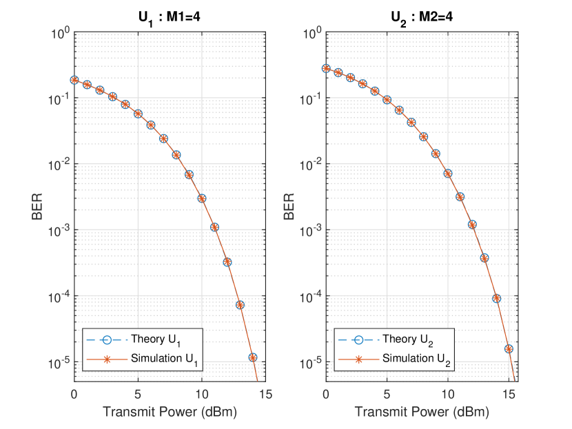
Figure 2: Average BER using $M_{1}=M_{2}$ for $U_{1}$ and $U_{2}$.

Proof:

As mentioned before, the probability of error for $U_{2}$ depends on $s^{\prime}_{1}$ which is the estimation of $U_{1}$’s symbol during the SIC. In [31] it is explained thoroughly how the error probability of each bit of $U_{2}$’s symbol is connected only with specific bits of the first users estimated symbol. Briefly, the bits of $U_{1}$’s symbol can be divided into two equal groups based on the nature of interference that they cause on the received signal. The first group can be the set of symbols that introduce interference at the real part of the received signal and the second group can contain the bits that introduce interference at the imaginary part of the signal. Each group of $U_{1}$’s bits can affect $\log_{2}\sqrt{M_{1}}$ bits of the second users symbol. Thus, the interference that is experienced during the demodulation of the $s_{2}$ symbol can be expressed as

$$I_{real,2}=\Re\left\{\big{(}\rho_{1}\big{|}\mathbf{h}_{2}^{H}\mathbf{u}_{1}\big{|}+\rho_{2}\big{|}\mathbf{h}_{2}^{H}\mathbf{u}_{2}\big{|}\big{)}s^{\prime}_{1}+\tilde{\nu}_{2}\right\},$$ (33)

for the bits of $s_{2}$ that are carried by the real part of $\tilde{y}_{2}$, and as

$$I_{imag,2}=\Im\left\{\big{(}\rho_{1}\big{|}\mathbf{h}_{2}^{H}\mathbf{u}_{1}\big{|}+\rho_{2}\big{|}\mathbf{h}_{2}^{H}\mathbf{u}_{2}\big{|}\big{)}s^{\prime}_{1}+\tilde{\nu}_{2}\right\}$$ (34)

for the bits of $s_{2}$ that are carried by the imaginary part of $\tilde{y}_{2}$. Expressions $S,D_{2},D_{3},L_{1,2}$ and $\Lambda_{n}$ define the number of $Q$-functions that will appear in each part of $P_{b,i}^{(2)}$ expression. In Appendix A we present the case of $M_{1}=M_{2}=4$ for QAM constellations in detail. Additionally, in Fig. 2 we can observe the analytical and the simulated BER of user $U_{1}$ for the aforementioned case.

∎

III-D BER optimization problem.

To ensure correct transmission and prevent any overlap among users’ symbols, it is necessary for the beamformer parameters to adhere to the following constraints. As we can observe in [32] the following rate has to be satisfied

$$\bigg{|}\frac{\rho_{1}}{\delta_{1}(\cos(\tau_{1})-\sin(\tau_{1}))\cdot\Lambda_{2}}\bigg{|}>Y_{1},$$ (35)

where $Y_{1}=\frac{M_{1}-1}{M_{2}-1}\cdot(\sqrt{M_{2}}-1)^{2}$.

Likewise, by following the analysis of the previous expressions, we reach to the conclusion that in order for the SIC to be reliable, the following expression also has to be valid

$$\frac{\rho_{1}\big{|}\mathbf{h}_{2}^{H}\mathbf{u}_{1}\big{|}+\rho_{2}\big{|}\mathbf{h}_{2}^{H}\mathbf{u}_{2}\big{|}}{\big{|}\delta_{1}e^{j\phi_{1}}\mathbf{h}_{2}^{H}\mathbf{u}_{1}+\delta_{2}e^{j\phi_{2}}\mathbf{h}_{2}^{H}\mathbf{u}_{2}\big{|}}>Y_{1}.$$ (36)

In addition to these restrictions, we have to consider that there are limitations on the maximum transmit power of our system. By normalizing the transmit power of the constraints in (16) to unity, we derive the following expression

$$\rho_{1}^{2}+\rho_{2}^{2}+\delta_{1}^{2}+\delta_{2}^{2}\leq 1.$$ (37)

Based on this derived framework, the search for beamforming vectors that provide the lowest possible maximum BER between the two users (16), comes down to finding the optimal $\rho_{i},\delta_{i},\tau_{i},\phi_{i}$ parameters and can be formulated as

$$\begin{split}{}&{}\operatorname*{arg\,min}_{\rho_{1},\rho_{2},\delta_{1},\delta_{2},\tau_{1},\phi_{1},\phi_{2}}\{\max\{P_{e}^{(1)},P_{e}^{(2)}\}\}\\ &\textrm{subject to:}\;\;\eqref{constr1},\;\eqref{constr2},\;\eqref{constr3}.\end{split}$$ (38)

It has to be noted that the objective function of our problem (38), is to find the maximum between two $Q$-function sums. It is known that the $Q$-function is neither convex nor concave, thus the problem can not be solved with conventional convex optimization techniques like the ones found in [33]. Therefore, in an effort to create a fast and robust system that can predict the optimal beamformer that achieves fairness between the users in terms of conditional BER, we apply Machine Learning techniques. Specifically, we use Neural Networks in order to learn the non-linear correlation that exists between the channel state information of the two users and the characteristics of their beamformers.

IV Proposed Learning Algorithm

In this section, we introduce the proposed learning algorithm that will be used for the selection of the beamforming parameters of each user. Our approach is based on using neural networks to learn the non-linear correlation mentioned above. In what follows, we separately discuss the several steps which are related to the design and application of our algorithm.

IV-A Generation of training/CSI data

In order to create the training data which are necessary for the training process, we generate random realizations of the channels formed between the Base Station (BS) and the two users, using the statistical channel model presented in (6). Such an approach is also followed in [19, 20, 21, 23, 34, 35, 36] for the purposes of designing ML-based resource allocation and signal processing algorithms. Following such an approach, allows us to apply our ML based methodology in the absence of real channel data. Moreover, in practice the Rayleigh fading channel model has been found to accurately model wireless/mobile propagation channels [37].

IV-B Solving the optimal beamforming problem for the training data

In order for our algorithm to learn how to infer beamforming decisions, the optimal beamformer decision for each one of the training CSI data is required. As a result for each one of the training data instances we need to solve the corresponding instance of problem (38). However, as already explained optimally solving problem (38) is not straightforward mainly due to the fact that the cost function is not convex. As a result, the application of any standard iterative algorithm for solving problem (38) is not guaranteed to provide the globally optimal solution. To overcome this problem, we solve problem (38) using a constraint optimization algorithm. More specifically, we use MATLAB’s optimization toolbox and the corresponding functions for constrained nonlinear multivariable problems. For each CSI instance, we apply the constrained optimization procedure from 20 random initial points and we keep the response that minimizes the maximum BER among the two users. This way, we create pairs of channel realizations and optimal beamforming vectors that constitute the inputs and the outputs of the neural network respectively. This proposed method cannot ensure that the global minimum will be found universally, but is able to choose the best solution out of several local minima.

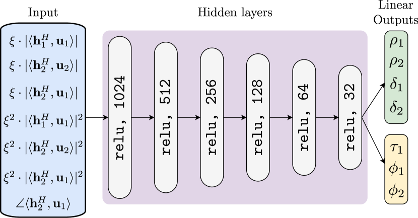
Figure 3: Architecture of the used Neural Network. In this figure we present the architecture of the proposed NN and give information about the shape of the input layers, the size and the activation functions of the hidden layers and the linear outputs that are formed by the two branches that exit the last hidden layer.

IV-C Selecting appropriate Neural Network architectures

The literature contains multiple proposals for solving the power allocation problem using deep neural networks (DNN). First, we can see in [19] the use of deep convolutional neural networks to perform min-max power allocation in a cell-free massive MIMO system. The use of convolutional layers is also met in [20], where the use of a residual network that consists of multiple convolutional and fully connected layers is used for power allocation in a multi-cell massive MIMO setup. The use of residual networks (ResNet) are commonly used in image recognition problems [38]. Specifically, in [39] a ResNet is used in order to predict angles, similar to the ones in our problem. Nevertheless, all these works use tend to use convolutional networks in order to exploit the spatial information hidden in the multidimensional data that they use as inputs. A characteristic that is not met in our work.

Another commonly used architecture of neural networks for power allocation is the fully connected one. In [23] a fully connected DNN is introduced with the aim of managing interference by approximating the WMMSE algorithm. This scheme uses as inputs of the DNN the magnitude of the channel realization and it achieves very good levels of performance. Additionally, feed forward neural networks with fully connected layers are used in [21, 34] and use vectors of user positions or shadowing coefficients in order to extract the optimal power allocation parameters.

Based on the previous analysis and according to the universal function approximation property [40, 41], our problem (38) can be solved with the use of a DNN. The model that we consider to be the most suitable for our case is a fully connected deep neural network. It consists of 6 hidden layers, the designated sizes of which are noted in Fig.3. All hidden layers will use the Rectified Linear Unit (ReLU) activation function. In order to decrease the network’s complexity and processing time, the architecture is partly shared between the two tasks. However, at the final stage, it is divided into two branches and forms the two outputs, as we can observe in Fig.3. The first branch of the output includes the four parameters that take values in the range $[0,1]$ (i.e. $\rho_{1},\rho_{2},\delta_{1},\delta_{2}$) and the second branch, includes the three angles that take values in the range $[0,2\pi)$ (i.e. $\tau_{1},\phi_{1},\phi_{2}$). Although the prediction of all these outputs is a regression problem, due to their different nature and value range, we propose the separation of the last layer into two independent compartments. This technique is used for the prediction of heterogeneous outputs from the same data as we can see in [39]. Both of NN outputs will use linear activation functions. Since the task that we are trying to accomplish is a regression problem, the mean absolute error (MAE) loss function is preferred by both outputs. Subsequently, the overall loss function of the neural network will be a weighted sum of the two individual losses. The algorithm that is used for the training of the neural network is the ADAM algorithm with Nesterov’s momentum [42, 43]. The training continues for maximum of 200 epochs, unless it meets the predetermined training conditions, where it stops automatically. Finally, the input of the DNN will consist of the magnitude and the angles of the dot products between the channel realizations of the two NOMA users and the vectors of the orthonormal basis, as presented in Fig.3. We note that we ignore some parts of the available information, such as the angles of $\langle\mathbf{h}_{1}^{H},\mathbf{u}_{1}\rangle$ and $\langle\mathbf{h}_{2}^{H},\mathbf{u}_{2}\rangle$ because they are equal to zero, due to the properties of the orthonormal basis. We use $\xi$ as an equalization factor, so that all the input components belong to similar orders of magnitude. Thus, the neural network will have the same input size for every different antenna scheme, with dimensions $7\times 1$. This property allows as to train a single neural network for all the different antenna schemes that we consider. It also enables the opportunity to use the same neural network in case that a new antenna scheme appears, just by merging the data from all the antennas schemes and retraining the same neural network.

Although we suggest a specific DNN structure, it is important to note that discovering the optimal neural network architecture can be viewed as a separate optimization problem that requires additional research. Based on the approximation and estimation bounds for NNs presented in [44] and the works of [41] in deep learning techniques, we experimented with various architectures of fully connected networks, aiming to find the best one in terms of MAE. The range of the fully connected NNs that we tested varies from two to six layers and consists of different numbers of neurons. During our tests, we also used various activation functions for the hidden layers, as well as for the output layer and different training algorithms. We also examined the use of two separate neural networks, one for each output and we compared these results with our proposed layout.

V Simulation & Numerical results

In order to evaluate the performance of the proposed learning algorithms we considered a scenario where a multi-antenna BS communicates with two users following the channel model presented in (6). Note that the specific channel model is part of 3GPP standard channel models [45]. As a result, it can be considered a good option for generating channel instances which preserve some of the properties of real channel data measurements: The remaining parameters of our simulation driven performance evaluation are presented in Table I. Concerning user placement, for our purposes, we have considered the case that $U_{1}$ is always located at a distance between 600 and 650 meters from the BS at each realization, and $U_{2}$ at a distance between 350 and 400 meters. Moreover, we have assumed that the modulation order of $U_{1}$ and $U_{2}$ is the same and is equal to $M=M_{1}=M_{2}=4$, while the noise variance was also assumed to be the same for both users and equal to $N_{0}\times B$, where $N_{0}$ the noise density and $B$ the system bandwidth, both given in Table I. For this particular simulation scenario, we have investigated the performance of our proposed algorithm, and compared it with commonly used beamformers, which serve as benchmarks for our algorithm. These beamformers are briefly presented in what follows.

TABLE I: Model parameters used in simulations

Parameter	Value
Carrier frequency	2GHz
System Bandwidth	10MHz
Noise power density	-174 dBm/Hz
Path-loss in dB	PL = 128.1 + 37.6$\log_{10}$d, d in km
Transmit power	100mW
$U_{1}$ distance	600m - 650m
$U_{2}$ distance	350m - 400m
$M_{1},M_{2}$	4

V-A The considered benchmarks

The beamforming algorithms which were compared, in terms of performance, to our proposed algorithm, were the following.

V-A1 Maximum Ratio Transmission (MRT)

In the case of MRT [46], the beamforming vector applied on the data of user $U_{k}$ is expressed as:

$$\mathbf{w}_{k}=\frac{\mathbf{h}_{k}}{||\mathbf{h}_{k}||}.$$ (39)

MRT beamforming aims at maximizing the SNR of the signal $s_{k}$ at user $U_{k}$. The main disadvantage of this approach is that it does not take into account the interference caused to the weak user, which can be large.

V-A2 Zero Forcing Beamforming (ZFBF)

ZFBF aims to create beamforming vectors that cause zero interference to other users [47]. To do so, the beamforming vectors that this technique creates are orthogonal to the channel vectors of all the users, but the one that transmits with it, as we observe in the following equations.

$$\mathbf{h}_{1}^{H}\mathbf{w}_{2}=0\;\;,\;\;\mathbf{h}_{2}^{H}\mathbf{w}_{1}=0.$$ (40)

The two aforementioned techniques will be used as follows. First, we will use MRT for both users, then the ZFBF, again for both users and finally, we will use combinations of these two choices between the users. That is, MRT for the first user and ZFBF for the second one and vice versa.

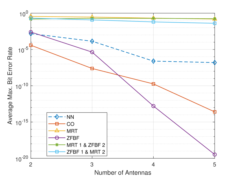
Figure 4: Comparison of the maximum BER of the two users for various beamforming techniques.

Figure 5: Histogram of the maximum BER of the two users.

Figure 6: Histogram of the maximum BER of the two users - zoomed.

In Fig.4 we can observe the average BER of all these four techniques, alongside with the results of the neural network and of the CO for the different antenna schemes. These BER values are the result of the averaging of thousand of different channel realizations for each antenna scheme. As we can see, CO outperforms all other techniques for a low number of antennas. We can see that ZFBF takes a steep increase in performance in terms of BER as the number of antennas increases. Next, the NN, improves its BER performance as the number of antennas increases. The rest of the techniques seem to perform poorly in all antenna cases.

Looking back on the ZFBF technique, we would like to make some comments. First of all, ZFBF as we use it can not be considered to be a NOMA technique, since it completely eliminates the interference of each user in the receiving signal of the other one. Nevertheless, in the figures that we present, ZFBF seems to be a good choice for a beamforming technique. Indeed, it seems to be a good solution, without needing the computational time of constraint optimization in order to find a good solution. We can also see, that as the number of transmitting antennas increases, the gap between ZFBF and any other technique increases. This is happening because ZFBF is based on the orthogonal relationship of the beamformers with the channel vectors of the other users. This property is enhanced as the number of transmitting antennas is increasing compared to the number of users and therefore the number of receive antennas since this increase offers more degrees of freedom at the beamforming vector. However, in multiple antenna NOMA systems, many user pairs or clusters coexist. In these cases, ZFBF is not used as a beamforming technique for each user of each cluster. Usually, it is used as the first step of the beamforming design in order to reduce inter-cluster interference. But again, in most of these cases, the number of users and receive antennas surpasses the number of transmit antennas. Thus, the zero - interference properties of ZFBF cannot be achieved even with ZFBF that tackles inter-cluster interference and therefore, this technique is considered suboptimal [8, 48].

We have to note that, although from the average BER of each scheme we can judge each technique, this judgment can be sometimes distorted since this representation technique is based on the mean values of the sizes and not on their distribution. A more accurate image can be seen with the use of histograms. In Fig.5 and Fig. 6 we can observe the histograms that present the maximum BER of the two users based on the beamforming technique used each time. The results that were used in order to generate these histograms consider a plethora of randomly positioned user pairs, as well as different antenna schemes (2,3,4 or 5 antennas at the BS). First of all we have to notice again the superiority of CO, NN and ZFBF against all other techniques. On the other hand, we have to notice that the judgment for the three other techniques is not the same as before. We can see that the poor average values that are presented in Fig.4 are not a result of the universally poor performance of these techniques. On the contrary, a big portion of their uses produces low maximum BERs, lower even that $10^{-5}$ as we can see in Fig.6. More specifically, the most characteristic case is the one of MRT, in which maximum BERs are mainly concentrated around very low or extremely high values. Similar behavior we also notice while we use the combinations of MRT and ZFBF. In these cases, more than half of the tested cases produce maximum BERs lower than $10^{-5}$, but a large number of them produces maximum BERs of the highest value. Going back to CO, NN and ZFBF, we can observe that the conclusions that we extract are different from the ones when looking to Fig.4. We can see that the difference in performance between these three techniques is not that big. CO has the most cases of maximum BER under 0.05 in Fig.5 and the biggest amount of cases under $10^{-5}$ as we can see in Fig.6. The neural network beamforming technique comes second in front of ZFBF in these metrics, something strange based on the results of Fig.4. A good explanation for these difference can be the existance of outliers in the results of CO and NN when compared with ZFBF. That is, that these two techniques have an extremely small number of cases, in which the maximum BER is very high, affecting the mean values of their BERs.

Figure 7: Performance comparison for the 3-antenna scheme between CO, universal NN and NN trained only with data from the 3-antenna scheme.

To conclude, CO can find suitable beamforming vectors by computing the parameters of the beamforming structure that we present in (17) and (18). With the help of the neural network that we proposed, these parameters can be learned and used to create beamforming vectors in any MISO-NOMA system that is based on user fairness. However, we need to emphasize on the time that these last two techniques (i.e. CO, NN) need in order to provide these results. The calculation of the optimal beamformer in our case is the task of constrained optimization with multiple random initialization points in a non-convex seven-dimensional space. In combination with the fact that the BER expressions consist of multiple sums, of which the derivatives have to be calculated, we understand that finding of the optimal solution through constrained optimization is a procedure that requires a lot of computational time. On the other hand, the use of pre-trained NN with size such as in our case is a robust procedure with very low complexity, that needs negligible time in order to provide responses. The robustness and efficiency of our NN based system can also be seen in Fig.7. Our algorithm enables the NN to be additionally trained with data from various antenna schemes. This is possible thanks to the use of the inner products between the channel vectors and the orthogonal basis vectors as inputs of the NN. With this technique, we can train a single NN for any number of antennas and use it universally with great results. In Fig.7 we can see that the use of the same NN for all the available antenna schemes does not affect at all the maximum BER performance of the system when compared with the NN that is trained only on the data from the 3-antenna scheme. On the contrary, it performs if anything equally well, and in our case it outperforms the single scheme trained NN, since it results to a few more cases in BER lower than $10^{-6}$.

VI Conclusion

In this paper, the closed-form expression of the BER for two users was expanded for the scenario of MISO-NOMA over Rayleigh channels. A new method of providing beamformers that grant fairness between the users was proposed, with the use of very simple and agile neural networks. This is a promising method that provides good results rapidly and with capabilities of easy scale for other use cases. We also saw that our system works successfully when different number of antennas used from the transmitter. A quality that brings the cost of training and deploying a system like this to minimum, as it is not necessary to use a different NN pair for each case. Finally, some extensions that we could explore in future works, are the scenarios with more users, as well as scenarios with use of real-time data.

Appendix A Example $M_{1}=M_{2}=4$

In this appendix we present the expressions of the conditional BER for the two users in the case of multiple antenna at BS (MISO - NOMA). We note that both users use a 4-QAM modulation, i.e. $M_{1}=M_{2}=4$.

A-A $U_{1}$ Expression

In this section, we present the expressions for the conditional BER, as an average of the probabilities of error for each bit of user $U_{1}$. First of all, the index representation of each bit will be $b_{1i}$, where $i$ is the index of the first user’s bits, with $i\in\{1,2,...,B_{1}\}$ and $B_{1}=\log_{2}M_{1}$. If we take as an example the case of $M_{1}=M_{2}=4$, we can create a constellation diagram such as in Fig. 8, where the $B_{1}=2$ first bits will represent $U_{1}$’s symbols and the rest will represent $U_{2}$’s ones.

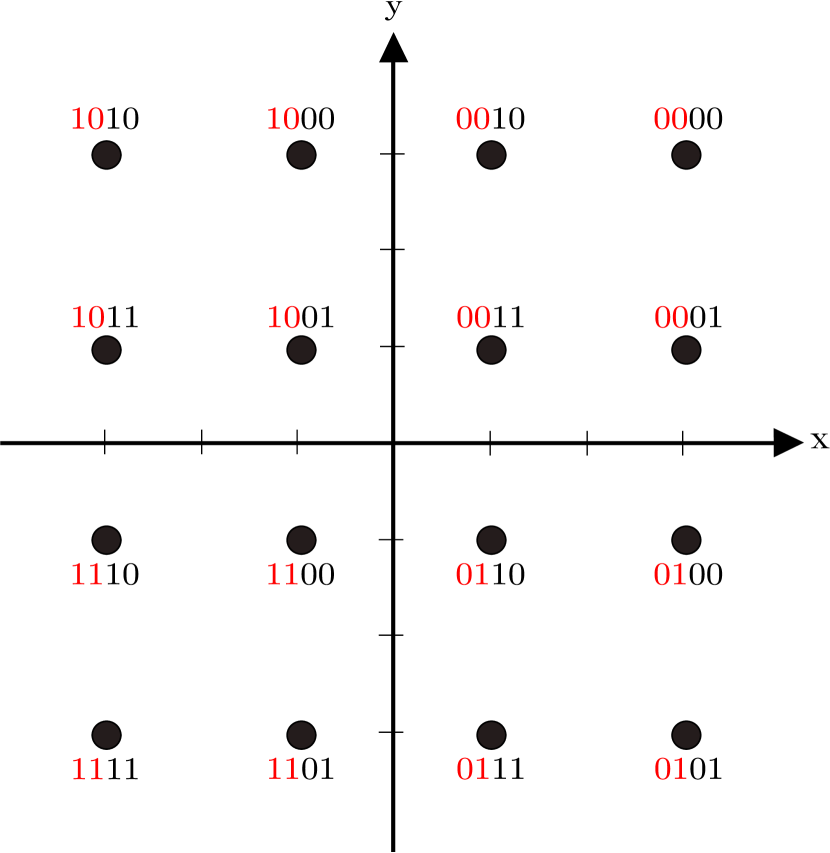
Figure 8: Constellation diagram of a NOMA symbol, (4-QAM modulation for both users).

It should be mentioned that the use of Gray coding allows the appearance of patterns, quite useful in the analysis of the multiple antenna scenario. Specifically, due to Gray coding, the BER expression is affected only by the real part of the interference and the noise for the first $B_{1}/2$ bits, while it is affected by the imaginary part of them for the remaining $B_{1}/2$ bits of the first user, as we can notice in Fig. 8. This phenomenon, in combination with the fact that $U_{1}$’s bits remain unchanged inside each quadrant, generates two properties that can be exploited for the benefit of the detection of $\hat{s}_{1}$ in (21). Initially, the $x$ and $y$ axes can be used as the decision boundaries of the two groups of $U_{1}$’s bits, respectively. Secondarily, the computation of the distances between all the feasible symbols and $\hat{s}_{1}$ can be done, either by choosing only 4 symmetrical symbols from the constellation, as seen clearly in Fig. 8. Due to these properties, the probability of error for the first $B_{1}/2$ bits is equal with probability of error with the second $B_{1}/2$ bits, with the only difference to be the decision boundary that we consider. Consequently, in our case the probability of error for $b_{11}$ is equal to the probability of error for $b_{12}$. Thus, the expression of BER for $U_{1}$ in the case of $M_{1}=M_{2}=4$ is

$$\begin{split}{}&{}P_{e}^{(1)}=\frac{1}{4}\bigg{[}Q(g_{1}\left(1,-1,-1\right))+Q(g_{1}\left(1,-1,1\right))\\ &\;\;\;\;\;\;\;\;\;\;\;\;+Q(g_{1}\left(1,1,-1\right))+Q(g_{1}\left(1,1,1\right))\bigg{]}.\end{split}$$ (41)

with $g_{1}$ as defined in (23).

A-B $U_{2}$ Expression

Previously, we explained the connection between the bits of the first users symbol that are estimated during the SIC and the bits of the $U_{2}$ symbol. Since both users’ constellation use Gray coding, we know that the probability of error for the $b_{21}$ and $b_{22}$ bits are equal. Thus, the average conditional BER expression of the second user for $M_{1}=M_{2}=4$ can be written as

$$\begin{split}{}&{}P_{e}^{(2)}=\frac{1}{2}\bigg{[}2Q(g^{+}_{2}(0,1))-Q(g^{+}_{2}(1,1))+Q(g^{+}_{2}(2,1))\\ &\;\;\;\;\;\;\;\;\;\;\;+Q(g^{-}_{2}(1,1))-Q(g^{-}_{2}(2,1))\bigg{]},\end{split}$$ (42)

with $g_{2,i}^{\pm}$ as defined in (32).

References

- [1] L. Dai, B. Wang, Y. Yuan, S. Han, I. Chih-lin, and Z. Wang, “Non-orthogonal multiple access for 5G: solutions, challenges, opportunities, and future research trends,” IEEE Communications Magazine, vol. 53, pp. 74–81, Sept. 2015.
- [2] Z. Ding, Y. Liu, J. Choi, Q. Sun, M. Elkashlan, I. Chih-Lin, and H. V. Poor, “Application of Non-Orthogonal Multiple Access in LTE and 5G Networks,” IEEE Communications Magazine, vol. 55, pp. 185–191, Feb. 2017.
- [3] W. Shin, M. Vaezi, B. Lee, D. J. Love, J. Lee, and H. V. Poor, “Non-Orthogonal Multiple Access in Multi-Cell Networks: Theory, Performance, and Practical Challenges,” IEEE Communications Magazine, vol. 55, pp. 176–183, Oct. 2017.
- [4] Z. Yang, Z. Ding, P. Fan, and N. Al-Dhahir, “A General Power Allocation Scheme to Guarantee Quality of Service in Downlink and Uplink NOMA Systems,” IEEE Transactions on Wireless Communications, vol. 15, pp. 7244–7257, Nov. 2016.
- [5] S. Islam and K. Kwak, “Outage capacity and source distortion analysis for NOMA users in 5G systems,” Electronics Letters, vol. 52, pp. 1344–1345, July 2016.
- [6] Z. Ding, P. Fan, and H. V. Poor, “Impact of User Pairing on 5G Nonorthogonal Multiple-Access Downlink Transmissions,” IEEE Transactions on Vehicular Technology, vol. 65, pp. 6010–6023, Aug. 2016.
- [7] Y. Liu, H. Xing, C. Pan, A. Nallanathan, M. Elkashlan, and L. Hanzo, “Multiple-Antenna-Assisted Non-Orthogonal Multiple Access,” IEEE Wireless Communications, vol. 25, pp. 17–23, Apr. 2018.
- [8] M. S. Ali, E. Hossain, and D. I. Kim, “Non-Orthogonal Multiple Access (NOMA) for Downlink Multiuser MIMO Systems: User Clustering, Beamforming, and Power Allocation,” IEEE Access, vol. 5, pp. 565–577, 2017.
- [9] F. Zhou, Z. Chu, H. Sun, and V. C. M. Leung, “Resource Allocation for Secure MISO-NOMA Cognitive Radios Relying on SWIPT,” in 2018 IEEE International Conference on Communications (ICC), (Kansas City, MO), pp. 1–6, IEEE, May 2018.
- [10] X. Wang, F. Labeau, and L. Mei, “Closed-Form BER Expressions of QPSK Constellation for Uplink Non-Orthogonal Multiple Access,” IEEE Communications Letters, vol. 21, pp. 2242–2245, Oct. 2017.
- [11] F. Kara and H. Kaya, “BER performances of downlink and uplink NOMA in the presence of SIC errors over fading channels,” IET Communications, vol. 12, pp. 1834–1844, Sept. 2018.
- [12] L. Bariah, S. Muhaidat, and A. Al-Dweik, “Error Probability Analysis of Non-Orthogonal Multiple Access Over Nakagami- Fading Channels,” IEEE Transactions on Communications, vol. 67, pp. 1586–1599, Feb. 2019.
- [13] J.-R. Garnier, A. Fabre, H. Fares, and R. Bonnefoi, “On the Performance of QPSK Modulation Over Downlink NOMA: From Error Probability Derivation to SDR-Based Validation,” IEEE Access, vol. 8, pp. 66495–66507, 2020.
- [14] H. Yahya, E. Alsusa, and A. Al-Dweik, “Exact BER Analysis of NOMA With Arbitrary Number of Users and Modulation Orders,” IEEE Transactions on Communications, vol. 69, pp. 6330–6344, Sept. 2021.
- [15] C. Zhang, P. Patras, and H. Haddadi, “Deep Learning in Mobile and Wireless Networking: A Survey,” IEEE Communications Surveys & Tutorials, vol. 21, no. 3, pp. 2224–2287, 2019.
- [16] N. Samuel, T. Diskin, and A. Wiesel, “Deep MIMO detection,” in 2017 IEEE 18th International Workshop on Signal Processing Advances in Wireless Communications (SPAWC), (Sapporo), pp. 1–5, IEEE, July 2017.
- [17] X. Yan, F. Long, J. Wang, N. Fu, W. Ou, and B. Liu, “Signal detection of MIMO-OFDM system based on auto encoder and extreme learning machine,” in 2017 International Joint Conference on Neural Networks (IJCNN), (Anchorage, AK, USA), pp. 1602–1606, IEEE, May 2017.
- [18] H. Ye, G. Y. Li, and B.-H. Juang, “Power of Deep Learning for Channel Estimation and Signal Detection in OFDM Systems,” IEEE Wireless Communications Letters, vol. 7, pp. 114–117, Feb. 2018.
- [19] Y. Zhao, I. G. Niemegeers, and S. H. De Groot, “Power Allocation in Cell-Free Massive MIMO: A Deep Learning Method,” IEEE Access, vol. 8, pp. 87185–87200, 2020.
- [20] T. Van Chien, T. Nguyen Canh, E. Bjornson, and E. G. Larsson, “Power Control in Cellular Massive MIMO With Varying User Activity: A Deep Learning Solution,” IEEE Transactions on Wireless Communications, vol. 19, pp. 5732–5748, Sept. 2020.
- [21] L. Sanguinetti, A. Zappone, and M. Debbah, “Deep Learning Power Allocation in Massive MIMO,” in 2018 52nd Asilomar Conference on Signals, Systems, and Computers, (Pacific Grove, CA, USA), pp. 1257–1261, IEEE, Oct. 2018.
- [22] M. A. Wijaya, K. Fukawa, and H. Suzuki, “Intercell-Interference Cancellation and Neural Network Transmit Power Optimization for MIMO Channels,” in 2015 IEEE 82nd Vehicular Technology Conference (VTC2015-Fall), (Boston, MA, USA), pp. 1–5, IEEE, Sept. 2015.
- [23] H. Sun, X. Chen, Q. Shi, M. Hong, X. Fu, and N. D. Sidiropoulos, “Learning to Optimize: Training Deep Neural Networks for Interference Management,” IEEE Transactions on Signal Processing, vol. 66, pp. 5438–5453, Oct. 2018.
- [24] G. Gui, H. Huang, Y. Song, and H. Sari, “Deep Learning for an Effective Non Orthogonal Multiple Access Scheme,” IEEE Transactions on Vehicular Technology, vol. 67, pp. 8440–8450, Sept. 2018.
- [25] J. G. Proakis and M. Salehi, Digital communications. Boston: McGraw-Hill, 5th ed ed., 2008. OCLC: 911062607.
- [26] H. Q. Ngo, A. Ashikhmin, H. Yang, E. G. Larsson, and T. L. Marzetta, “Cell-Free Massive MIMO Versus Small Cells,” IEEE Transactions on Wireless Communications, vol. 16, pp. 1834–1850, Mar. 2017.
- [27] F. Alavi, K. Cumanan, Z. Ding, and A. G. Burr, “Beamforming Techniques for Non Orthogonal Multiple Access in 5G Cellular Networks,” IEEE Transactions on Vehicular Technology, vol. 67, no. 10, pp. 9474–9487, 2018.
- [28] J. Choi, “On generalized downlink beamforming with NOMA,” Journal of Communications and Networks, vol. 19, pp. 319–328, Aug. 2017.
- [29] G. A. Ropokis, “Multi-relay cooperation with self-energy recycling and power consumption considerations,” in 2019 International Conference on Wireless and Mobile Computing, Networking and Communications (WiMob), (Barcelona, Spain), pp. 268–275, IEEE, Oct. 2019.
- [30] O. T. Demir and T. E. Tuncer, “Optimum QoS-Aware Beamformer Design for Full-Duplex Relay With Self-Energy Recycling,” IEEE Wireless Communications Letters, vol. 7, pp. 122–125, Feb. 2018.
- [31] T. Assaf, A. J. Al-Dweik, M. S. E. Moursi, H. Zeineldin, and M. Al-Jarrah, “Exact Bit Error-Rate Analysis of Two-User NOMA Using QAM With Arbitrary Modulation Orders,” IEEE Communications Letters, vol. 24, pp. 2705–2709, Dec. 2020.
- [32] I.-H. Lee and J.-B. Kim, “Average Symbol Error Rate Analysis for Non-Orthogonal Multiple Access With -Ary QAM Signals in Rayleigh Fading Channels,” IEEE Communications Letters, vol. 23, pp. 1328–1331, Aug. 2019.
- [33] S. P. Boyd and L. Vandenberghe, Convex optimization. Cambridge: Cambridge Univ. Press, 18. print ed., 2015.
- [34] C. D’Andrea, A. Zappone, S. Buzzi, and M. Debbah, “Uplink Power Control in Cell-Free Massive MIMO via Deep Learning,” in 2019 IEEE 8th International Workshop on Computational Advances in Multi-Sensor Adaptive Processing (CAMSAP), (Le Gosier, Guadeloupe), pp. 554–558, IEEE, Dec. 2019.
- [35] W. Xia, G. Zheng, Y. Zhu, J. Zhang, J. Wang, and A. P. Petropulu, “A deep learning framework for optimization of miso downlink beamforming,” IEEE Transactions on Communications, vol. 68, no. 3, pp. 1866–1880, 2020.
- [36] J. Kim, H. Lee, S.-E. Hong, and S.-H. Park, “Deep learning methods for universal miso beamforming,” IEEE Wireless Communications Letters, vol. 9, no. 11, pp. 1894–1898, 2020.
- [37] D. Tse and P. Viswanath, Fundamentals of Wireless Communication. Cambridge University Press, 1 ed., May 2005.
- [38] K. He, X. Zhang, S. Ren, and J. Sun, “Deep Residual Learning for Image Recognition,” in 2016 IEEE Conference on Computer Vision and Pattern Recognition (CVPR), (Las Vegas, NV, USA), pp. 770–778, IEEE, June 2016.
- [39] A. Loquercio, A. I. Maqueda, C. R. del Blanco, and D. Scaramuzza, “DroNet: Learning to Fly by Driving,” IEEE Robotics and Automation Letters, vol. 3, pp. 1088–1095, Apr. 2018.
- [40] K. Hornik, M. Stinchcombe, and H. White, “Multilayer feedforward networks are universal approximators,” Neural Networks, vol. 2, pp. 359–366, Jan. 1989.
- [41] I. Goodfellow, Y. Bengio, and A. Courville, Deep Learning. MIT Press, 2016. http://www.deeplearningbook.org.
- [42] I. Sutskever, J. Martens, G. Dahl, and G. Hinton, “On the importance of initialization and momentum in deep learning,” in Proceedings of the 30th International Conference on Machine Learning (S. Dasgupta and D. McAllester, eds.), vol. 28 of Proceedings of Machine Learning Research, (Atlanta, Georgia, USA), pp. 1139–1147, PMLR, June 2013. Issue: 3.
- [43] T. Dozat, “Incorporating Nesterov Momentum into Adam,” 2016.
- [44] A. R. Barron, “Approximation and estimation bounds for artificial neural networks,” Machine Learning, vol. 14, pp. 115–133, Jan. 1994.
- [45] 3GPP, “Evolved Universal Terrestrial Radio Access (E-UTRA); Radio Frequency (RF); system scenarios,” Technical Report (TR) 36.942, 3rd Generation Partnership Project (3GPP), 04 2022. Version 17.0.0.
- [46] T. Lo, “Maximum ratio transmission,” IEEE Transactions on Communications, vol. 47, pp. 1458–1461, Oct. 1999.
- [47] E. Björnson, “Optimal Resource Allocation in Coordinated Multi-Cell Systems,” Foundations and Trends® in Communications and Information Theory, vol. 9, no. 2-3, pp. 113–381, 2013.
- [48] J. Choi, “Minimum Power Multicast Beamforming With Superposition Coding for Multiresolution Broadcast and Application to NOMA Systems,” IEEE Transactions on Communications, vol. 63, pp. 791–800, Mar. 2015.