Incremental 3D Semantic Scene Graph Prediction from RGB Sequences

Abstract

3D semantic scene graphs are a powerful holistic representation as they describe the individual objects and depict the relation between them. They are compact high-level graphs that enable many tasks requiring scene reasoning. In real-world settings, existing 3D estimation methods produce robust predictions that mostly rely on dense inputs. In this work, we propose a real-time framework that incrementally builds a consistent 3D semantic scene graph of a scene given an RGB image sequence. Our method consists of a novel incremental entity estimation pipeline and a scene graph prediction network. The proposed pipeline simultaneously reconstructs a sparse point map and fuses entity estimation from the input images. The proposed network estimates 3D semantic scene graphs with iterative message passing using multi-view and geometric features extracted from the scene entities. Extensive experiments on the 3RScan dataset show the effectiveness of the proposed method in this challenging task, outperforming state-of-the-art approaches. Our implementation is available at https://shunchengwu.github.io/MonoSSG.

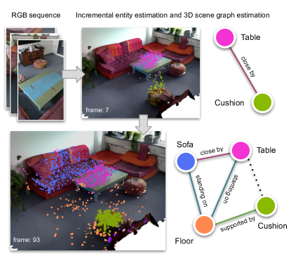
Figure 1: We propose a real-time 3D semantic scene graph estimation method that relies on an abstract understanding of a scene geometry built with RGB input. Our method estimates scene graphs incrementally by continuously estimating scene graphs and fusing local predictions into a global 3D scene graph.

1 Introduction

Scene understanding is a cornerstone in many computer vision applications requiring perception, interaction, and manipulation, such as robotics, AR/VR and autonomous systems [56, 54, 17, 55]. Semantic Scene Graphs (SSGs) go beyond recognizing individual entities (objects and stuff) by reasoning about the relationships among them [66, 61]. They also proved to be a valuable representation for complex scene understanding tasks, such as image captioning [67, 26], generation[24, 13], scene manipulation[10, 11], task planning [27], and surgical procedure estimation [42, 43]. Given the benefits of such representations, scene graph estimation received increasing attention in the computer vision community.

While earlier methods mainly estimate SSGs from images [18, 19, 72, 33, 66], recent approaches have also investigated estimating them from 3D data. Compared to 2D scene graphs, which describe a single image, 3D scene graphs depict the entire 3D scenes, enabling applications requiring a holistic understanding of the whole scene, such as path planning [47], camera localization, and loop closure detection [23]. However, existing 3D methods either require dense 3D geometry of the scenes to estimate 3D scene graphs [1, 61, 64, 23], which limits the use case since dense geometry is not always available, or constraints the scene graph estimation at the image-level [66, 15, 27], which tend to fail inferring relationships among objects beyond the individual viewpoints. A method that estimates 3D scene graphs relies on sparse scene geometry and reasoning about relationships globally has not been explored yet.

In this work, we propose a real-time framework that incrementally estimates a global 3D SSG of a scene simply requiring an RGB sequence as input. The process is illustrated in Fig. 1. Our method simultaneously reconstructs a segmented point cloud while estimating the SSGs of the current map. The estimations are bound to the point map, which allows us to fuse them into a consistent global scene graph. The segmented map is constructed by fusing entity estimation from images to the points estimated from a sparse Simultaneous Localization and Mapping (SLAM) method [3]. Our network takes the entities and other properties extracted from the segmented map to estimate 3D scene graphs. Fusing entities across frames is non-trivial. Existing methods often rely on dense inputs [58, 38] and struggle with sparse inputs since the points are not uniformly distributed. Estimating scene graphs with sparse input points is also challenging. Sparse and ambiguous geometry renders the node representations unreliable. On the other hand, directly estimating scene graphs from 2D images ignores the relationship beyond visible viewpoints. We aim to overcome the aforementioned issues by proposing two novel approaches. First, we propose a confidence-based fusion scheme which is robust to variations in the point distribution. Second, we present a scene graph prediction network that mainly relies on multi-view images as the node feature representation. Our approach overcomes the need for exact 3D geometry and is able to estimate relationships without view constraints. In addition, our network is flexible and generalizable as it works not only with sparse inputs but also with dense geometry.

We comprehensively evaluate our method on the 3D SSG estimation task from the public 3RScan dataset [60]. We experiment and compare with three input types, as well as 2D and 3D approaches. Moreover, we provide a detailed ablation study on the proposed network. The results show that our method outperforms all existing approaches by a significant margin. The main contributions of this work can be summarized as follows: (1) We propose the first incremental 3D scene graph prediction method using only RGB images. (2) We introduce an entity label association method that works on sparse point maps. (3) We propose a novel network architecture that generalizes with different input types and outperforms all existing methods.

2 Related Work

2.1 3D Object Localization from Images

Localizing 3D objects from images aims to predict the position and orientation of objects. Existing methods can be broadly divided into two categories: without and with explicit geometrical reasoning.

In the former category, many works focus on estimating 3D bounding boxes by extending 2D detectors with learned priors [28, 37, 41, 70]. When sequential input is available, single view estimations can be fused to estimate a consistent object map [2, 22, 29, 30]. However, the fused results may not fulfill the multi-view geometric constraints. Multi-view approaches estimate oriented 3D bounding boxes from the given 2D detection of views. They mainly focus on minimizing the discrepancies between the projected 3D representation and the detected 2D bounding boxes.

In the latter category, 3D objects are localized with the help of explicit geometric information. Many existing methods treat object detection as spatial landmarks in a map [21, 35, 40, 53, 65, 69], also known as object-level SLAM. Others focus on fusing dense per-pixel predictions to a reconstructed map [36, 6, 38, 71, 44, 16], which is known as semantic mapping or semantic SLAM.

A major difference between object-level and semantic SLAM is that the former focuses only on foreground objects, while the latter also considers the structural and background information. Specifically, SemanticFusion [36] fuses dense semantic segments from images to a consistent dense 3D map with Bayesian updates. Its map representation provides a dense semantic understanding of a scene ignoring individual instances. PanopticFusion [38] proposes to combine the instance and semantic segmentation from images to a panoptic map. Their approach considers foreground object instances and non-instance semantic information from the background. SceneGraphFusion [64] relies on 3D geometric segmentation [59] and scene graph reasoning to achieve instance understanding of all entities in a scene.

One significant difficulty in instance estimation for semantic SLAM is associating the instances across frames. Existing approaches mainly rely on a dense map to associate predictions by calculating the intersection-over-union (IoU) or the overlapping ratio between the input and the rendered image from the map. However, these methods produce sub-optimal results when the map representation is sparse due to the non-uniform distribution of the map points. We overcome this problem by proposing a confidence-based association.

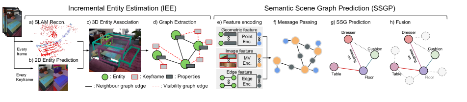
Figure 2: Given a sequence of RGB images, we use every frame to reconstruct a sparse point map (a) and every keyframe to estimate the 2D entities (b). (a) and (b) are associated and merged into a single 3D map (c). We asynchronously extract graph properties from the entity map (d) to estimate SSG. Our network computes the geometric, multi-view, and edge features (e). These features are propagated to each other with message passing (f), then used to predict a SSG (g). Then, periodic SSGs are fused to a global 3D SSG (h).

2.2 3D Semantic Scene Graph

Estimating 3D scene graphs methods can be divided according to various criteria. From the perspective of the scene graph structure, some methods focus on hierarchical scene graphs [1, 48, 50, 23]. These approaches mainly address the problem of relationship estimation between entities from different hierarchical levels, e.g. object, and room level. The other methods focuses on pairwise relationships, e.g. support and comparative relationships, between nodes within a scene [61, 27, 66, 64]. From the perspective of input data, some previous methods rely on RGB input [15, 27] by fusing 2D scene graph predictions to a consistent 3D map. On the other hands, other methods rely on 3D input [1, 48, 61, 50, 64, 23] by using known 3D geometries. Nevertheless, most of the existing methods estimate scene graphs offline [15, 1, 49, 48], while a few works [27, 64, 23] predict scene graph in real-time.

Among all existing work, the pioneering work in 3D scene graph estimation is proposed by [15]. The authors extend the 2D scene graph estimation method from [66] with temporal consistency across frames and use geometric features from ellipsoids. Kim et al. [27] propose an incremental framework to estimate 3D scene graphs from 2D estimations. Armeni et al. [1] are the first work to estimate 3D scene graphs through the hierarchical understanding of the scene. Rosinol et al. [48] build on top of [1] to capture moving agents. This work is subsequently extended to a SLAM system [50]. Wald et al. [61] propose the first 3D scene graph method based on the relationship between objects at the same level, along with 3RScan: a richly annotated 3D scene graph dataset. Wu et al. [64] extend [61] to real-time scene graph estimation with a novel feature aggregation mechanism. Hughes et al. [23] propose to reconstruct a 3D hierarchical scene graph in real-time incrementally. Our method incrementally estimates a flat scene graph with multi-view RGB input and a sparse 3D geometry, which differentiates our work from the previous methods relying on 3D input [61, 64], and approaches without geometric understanding [15, 27].

3 Method

The proposed framework is illustrated in Fig. 2, which shows how, given a sequence of RGB images, it can estimate a 3D semantic scene graph incrementally. The Incremental Entity Estimation (IEE) front end makes use of the images to generate segmented sparse points. Those are merged into 3D entities and used to generate both an entity visibility graph and a neighbour graph. The Semantic Scene Graph Prediction (SSGP) network uses the entities and both graphs to estimate multiple scene graphs and then fuse them into a consistent 3D SSG.

We define a SSG as $\mathcal{G}_{s}=\left(\mathcal{V},\mathcal{E}\right)$, where $\mathcal{V}$ and $\mathcal{E}$ denote a set of entity nodes and directed edges. Each node $v_{i}\in\mathcal{V}$ is assigned an entity label $l_{i}\in L$, a set of points $\mathcal{P}_{i}$, an Oriented Bounding Box (OBB) $b_{i}$ and a node category $c^{\text{node}}_{i}\in\mathcal{C}^{\text{node}}$. Each edge $e_{i\to j}\in\mathcal{E}$, connecting node $v_{i}$ to $v_{j}$ where $i\neq j$, consists of an edge category $c^{\text{edge}}_{i\to j}\in\mathcal{C}^{\text{edge}}$. $L$, $\mathcal{C}^{\text{node}}$, and $\mathcal{C}^{\text{edge}}$ denote all entity labels, a node category set, and an edge category set, respectively. An OBB $b_{i}$ is a gravity-aligned 3D bounding box consisting of a boundary dimension $\mathbf{b}_{i}\in\mathbb{R}^{3}$, a center $\mathbf{o}_{i}\in\mathbb{R}^{3}$, and an angle that encodes the rotation along the gravity axis. The OBBs are used to build both graphs and features. The entity visibility graph models the visibility relationship of the entities as a bipartite graph $\mathcal{G}_{c}=(\mathcal{V},\mathcal{K},\mathcal{E}_{c})$ where $\mathcal{K}$, $\mathcal{E}_{c}$ denote a set of keyframes and visibility edges, respectively. $\mathcal{G}_{c}$ gives the knowledge of the visibility of entity nodes in keyframes, which is used in computing multi-view visual features in SSGP. The neighbour graph encodes the proximity relationship of the entities as an undirected graph $\mathcal{G}_{p}=(\mathcal{V},\mathcal{E}_{p})$, where $\mathcal{E}_{p}$ is the set of proximity edges. The neighbour graph also serves as the initial graph for the message propagation step in SSGP.

3.1 Incremental Entity Estimation

During the first step of the IEE front end pipeline, a set of labeled 3D points are estimated from the sequence of RGB images (Sec. 3.1.1). The entity labels are determined using an entity segmentation method on selected keyframes (Sec. 3.1.2). Then, they are associated and fused into a sparse point map (Sec. 3.1.3). Finally, the entities and their properties are extracted using the labeled 3D points (Sec. 3.1.4).

3.1.1 Sparse Point Mapping

We use ORB-SLAM3 [3] to simultaneously estimate the camera poses and build a sparse point map by matching estimated keypoints from sequential RGB frames. To guarantee real-time performance, an independent thread is used to run the local mapping process using the stored keyframes. The same thread additionally takes care of running the entity detector and performing the label mapping process. For each point $\mathbf{p}_{m}\in\mathbf{P}$ in the map, we store its 3D coordinates, an entity label $l_{m}$, and its confidence score $w_{m}\in\mathbb{R}_{\geq 0}$.

3.1.2 2D Entity Detection

We estimate an entity label mask $\tilde{M}_{t}(u)\in\tilde{L}_{t}$ and a confidence mask $\tilde{W}_{t}(u)\in[0,1]\subset\mathbb{R}$ with every given keyframe $k_{t}\in\mathcal{K}$, where $u\in\mathbb{R}^{2}$ denotes the image coordinates and $\tilde{L}_{t}$ all entity labels in $k_{t}$. Both masks are estimated using a class-agnostic segmentation network which further improves other instance segmentation methods [4, 7, 31] by enabling the discovery of unseen entities [46, 25, 14]. Although segmentation networks provide accurate masks, the estimations are independent across frames. Thus, a label association stage is required to build a consistent label map.

3.1.3 Label Association and Fusion

Inspired by [58, 51, 35, 38], we use the reference map approach to handle the label inconsistency. It relies on a map reconstruction to solve label consistency by comparing input label mask to rendered mask. Then fuse the associated mask to the global point map.

Label Association. We start by building a reference entity mask $M_{t}(u)\in L$ by projecting point entity labels from the sparse point map using the pose of $k_{t}$. The consistency-resolved entity mask ${\hat{M}}^{\prime}_{t}(u)$ is estimated by evaluating the corresponding labels on the image mask $\tilde{M}_{t}(u)$ and the reference mask $M_{t}(u)$. This evaluation can be performed by different methods such as using intersection over union statistics [38] or the maximum overlapping ratio between label masks [58]. However, both methods assume that points are uniformly distributed; a premise that fails in most sparse point reconstruction tasks. In such cases, these methods become unstable, as shown in the example provided in the supplementary material. To overcome this problem, we propose to use the maximum mean confidence as the criteria to find the best candidate. First, a confidence mask $W_{t}(u)$ is built by projecting the point label confidence using the pose of $k_{t}$, then the mean confidence score of a label $\tilde{l}\in\tilde{M}_{t}(u)$ and a reference label $l\in M_{t}(u)$ is computed by

$$\bar{\mathbf{M}}(\tilde{l},l)=\frac{\sum_{u^{\prime}\in\mathbf{\Pi}(\tilde{l},l)}W_{t}(u^{\prime})}{\mathbf{\#}\left(\mathbf{\Pi}(\tilde{l},l)\right)},$$ (1)

where $\mathbf{\Pi}(\tilde{l},l)$ gives a set of image coordinates $u^{\prime}\in\mathbb{R}^{2}$ where $\tilde{l}$ and $l$ overlap: $\{u^{\prime}\mid({\tilde{M}_{t}(u^{\prime})=\tilde{l}})\land({M_{t}(u^{\prime})=l})\}$, and $\mathbf{\#}\left(\cdot\right)$ is the cardinality operator. Then, the mask ${\hat{M}}^{\prime}_{t}(u)$ is generated by replacing the per-pixel entity label $\tilde{l}\in\tilde{M}_{t}(u)$ with either a reference label $l$ or a new label $l_{\text{new}}\notin L$ depending on:

$$\tilde{l}=\begin{cases}{\arg\max}_{l}~{}\bar{\mathbf{M}}(\tilde{l},l)&\text{if }{\max}_{l}~{}{\frac{\mathbf{\#}\left(\mathbf{\Pi}(\tilde{l},l)\right)}{\mathbf{\#}\left(M_{t}(u)=l\right)}}>\tau\\ l_{\text{new}}&\text{otherwise}\end{cases},$$ (2)

where we filter out a match if the number of overlapped pixel has a low coverage over the total number of label $l$ on the reference mask with a threshold $\tau$. In addition, similar to [38], a reference entity label is assigned to only one input entity label. If a reference label has been assigned, we use descending order to search for the next best candidate.

Label Fusion. After the association process, the associated entity labels ${\hat{M}}^{\prime}_{t}(u)$ are fused to the sparse point map $\mathbf{P}$. Since each label on ${\hat{M}}^{\prime}_{t}(u)$ sources from a map point, the label and confidence value of a point are updated by

$$w_{\psi\left(u\right)}=\begin{cases}w_{\psi\left(u\right)}+\tilde{W}_{t}\left(u\right)&\text{if }M_{t}\left(u\right)={\hat{M}}^{\prime}_{t}\left(u\right)\\ w_{\psi\left(u\right)}-\tilde{W}_{t}\left(u\right)&\text{otherwise}\end{cases},$$ (3)

where $\psi(u)$ is the corresponding point index that is projected on the pixel location $u$ on both $M_{t}(u)$ and $W_{t}(u)$. In particular, when $w_{\psi(u)}<0$, we set the entity label $l_{\psi(u)}$ to ${\hat{M}}^{\prime}_{t}(u)$, and the weight $w_{\psi(u)}$ to $\tilde{W}_{t}(u)$.

3.1.4 Extraction

We use the points belonging to each entity label to compute the 3D OBB $b_{i}$ of an entity $v_{i}\in\mathcal{V}$. We perform statistical outlier removal (from PCL [52]) to filter out points that could lead to distorted boxes. For the computation, we make use of the minimum volume estimation method [5] assuming gravity alignment.

The entity visibility graph $\mathcal{G}_{c}=(\mathcal{V},\mathcal{K},\mathcal{E}_{c})$ consists of all nodes $\mathcal{V}$ and keyframes $\mathcal{K}$ connected by visibility edges $\mathcal{E}_{c}$. A visibility edge $e_{ij}\in\mathcal{E}_{c}$ exists if entity $v_{i}\in\mathcal{V}$ is visible in keyframe $k_{j}\in\mathcal{K}$. Specifically, the visibility is determined by checking if any point in node $v_{i}$ is visible at $k_{j}$.

The neighbour graph $\mathcal{G}_{p}=(\mathcal{V},\mathcal{E}_{p})$ consists of nodes $\mathcal{V}$ and its proximity edges $\mathcal{E}_{p}$. A proximity edge $e_{i\to j}\in\mathcal{E}_{p}\mid v_{i},v_{j}\in\mathcal{V},i\neq j$ exists if nodes $v_{i},v_{j}$ are close in space, which is determined using a bounding box collision detection method. Since the size of the OBBs is not precise, we extend their dimensions by a margin $\tau^{C}$ to include additional potential neighbours.

3.2 Semantic Scene Graph Prediction

For every of the scene extractions obtained by the IEE front end, SSGP estimates 3D semantic scene graphs using message passing to jointly update initial feature representations and relationships  [66, 15, 61, 64]. In the last step, the network fuses all of them into a consistent global 3D SSG. The initial node features are computed with multi-view image features (Sec. 3.2.1), while the initial edge feature is computed with the relative geometric properties of its connected two nodes (Sec. 3.2.2). Both initial features are jointly updated with a GNN along the connectivity given by the neighbour graph (Sec. 3.2.3). The updated node and edge are used to estimate their class distribution (Sec. 3.2.4). We apply a temporal scene graph fusion procedure to combine the predictions into a global 3D SSG (Sec. 3.2.5).

Our network architecture combines the benefits of 2D and 3D scene graph estimation methods by using 2D image features and 3D edge embedding. Image features are generally a better scene representation than 3D features, while using edge embedding in 3D allows performing relationship estimation without the constraint of the field of view. The effects of 2D and 3D features are compared in Sec. 4.2.

3.2.1 Node Feature

For each node $v_{i}\in\mathcal{V}$, we compute a multi-view image feature $\mathbf{v}_{i}$ and a geometric feature $\mathbf{g}_{i}$. We use the former as the initial node feature $\mathbf{f}^{v}_{i}=\mathbf{v}_{i}$ and include the latter with a learnable gate in the message passing step (Sec. 3.2.3).

The multi-view image feature is computed by aggregating multiple observations of $v_{i}$ on images given by the entity visibility graph. For each view, an image feature is extracted with an image encoding network given the Region-of-Interest (ROI) of the node. The image features are aggregated using a mean operation to the multi-view image feature $\mathbf{v}_{i}$. Although there are sophisticated methods to compress multi-view image features, such as using gated averaging [15] and learning a canonical representation [63], we empirically found that averaging all the input features [57] yields the best result (see supplementary material). The mean operation also allows incrementally computing the multi-view image feature with a simple moving average. The geometric feature $\mathbf{g}_{i}$ is computed from the point set $\mathcal{P}_{i}$ using a simple point encoder [45].

3.2.2 Edge Feature

For each edge $e_{i\to j}\in\mathcal{E}_{p}$, an edge feature $\mathbf{f}^{e}_{i\to j}$ is computed using the node properties from its connected two nodes $v_{i}$ and $v_{j}$ by

$$\mathbf{f}^{e}_{i\to j}=g_{s}\left(\left[\mathbf{o}_{j}-\mathbf{o}_{i},\mathbf{b}_{j}-\mathbf{b}_{i},R_{i\to j}\right]\right),$$ (4)

where $g_{s}\left(\cdot\right)$ is a Multilayer Perceptron (MLP), $[\cdot]$ denotes a concatenation function, and $R_{i\to j}$ is a relative pose descriptor which encodes the relative angle between two entities.

The relative pose descriptor is designed to implicitly encode relative angles between two nodes. Using an explicit one is not optimal since OBB estimations do not return the exact pose of an object, which makes explicit pose descriptor not applicable. We instead use the relative geometry properties on a reference frame constructed by the two nodes to implicitly encode the relative pose, as illustrated in Fig. 3. First, we construct a reference frame with the origin the midpoint of the center of two nodes, the x-axis to $\mathbf{o}_{j}$, the y-axis to the inverse of the gravity direction, and the z-axis the cross product of the x-axis and y-axis. Second, we take maximum and minimum values on each axis of the reference frame to compute the relative pose descriptor as

$$R_{i\to j}=\log\left(\left|\left[\mathbf{p}^{\text{max}}_{i}\oslash\mathbf{p}^{\text{max}}_{j},\mathbf{p}^{\text{min}}_{i}\oslash\mathbf{p}^{\text{min}}_{j}\right]\right|\right),$$ (5)

where $\oslash$ is the Hadamard division, $\mathbf{p}^{\text{max}}_{\square},\mathbf{p}^{\text{min}}_{\square}\in\mathbb{R}^{3}$ are the maximum and minimum points on the reference frame for $\square\in(i,j)$. We use an absolute logarithm ratio to improve the numerical stability.

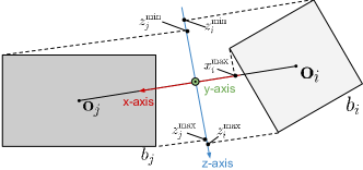
Figure 3: An illustration of our relative pose descriptor. The descriptor describe the relative maximum and minimum value of given two bounding boxes on a reference frame.

3.2.3 Message Passing

Given an initial node feature $\mathbf{f}^{v}_{i}$ and an edge feature $\mathbf{f}^{e}_{i\to j}$, we aggregate the messages from the neighbors for both nodes and edges to enlarge the receptive field and leverage the spatial understanding composition of the environment. We follow [66] by aggregating the messages with a respective GRU unit shared for all nodes and edges. Following, we explain the process taking place in each of the message-passing layers.

First, we incorporate the geometric feature to each node feature using a learnable gate:

$$\hat{\mathbf{f}}^{v}_{i}=\mathbf{f}^{v}_{i}+\sigma\left(\mathbf{w}^{T}[\mathbf{f}^{v}_{i},\mathbf{g}_{i}]\right)\sigma(\mathbf{g}_{i}),$$ (6)

where $\hat{\mathbf{f}}^{v}_{i}$ is the enhanced node feature, $\sigma$ denotes a sigmoid function, and $\mathbf{w}^{T}$ are learnable parameters. The geometric feature may be unreliable, especially when the input geometry is ambiguous or unstable. Thus, we use the learnable gate to learn if the feature should be included. A node message $m_{i}$ and an edge message $m_{i\to j}$ are computed by

$$m_{i}=g_{v}\left(\left[\hat{\mathbf{f}}^{v}_{i},\max_{j\in\mathcal{N}(i)}\left(\text{FAN}\left(\hat{\mathbf{f}}^{v}_{i},\mathbf{f}^{e}_{i\to j},\hat{\mathbf{f}}^{v}_{j}\right)\right)\right]\right),$$ (7)

$$m_{i\to j}=g_{e}\left([\hat{\mathbf{f}}^{v}_{i},\mathbf{f}^{e}_{i\to j},\hat{\mathbf{f}}^{v}_{j}]\right),$$ (8)

where $g_{v}\left(\cdot\right)$ and $g_{e}\left(\cdot\right)$ are MLPs, $\mathcal{N}(i)$ is the set of indices representing the neighbouring nodes of $i$, FAN is the feature-wise attention network [64] which weights all neighbour node feature $\hat{\mathbf{f}}^{v}_{j}$ using input query $\hat{\mathbf{f}}^{v}_{i}$, and key $\mathbf{f}^{e}_{i\to j}$ given $j\in\mathcal{N}(i)$.

3.2.4 Class Prediction and Loss Functions

We use the softmax function to estimate the class distribution on both nodes and edges. For multiple predicate estimations, we use the sigmoid function (with a threshold of 0.5) to estimate whether a predicate exists. The network is trained with a cross-entropy loss for classifying both entities and edges. The loss for the edge class is replaced with binary cross entropy for multiple predicates estimation [61].

3.2.5 Fusion

Multiple predictions on the same nodes and edges are fused to ensure temporal consistency. We use the running average approach [8] to fuse predictions [64]. For each entity and edge, we store the full estimated probability estimation $\boldsymbol{\mu}^{t}$ and a weight $\rho^{t}\in\mathbb{R}_{\geq 0}$ at time $t$. Given a new prediction, we update the previously stored $\boldsymbol{\mu}^{t-1}$ and $\rho^{t-1}$ as

$$\boldsymbol{\mu}^{t}=\frac{\boldsymbol{\mu}^{t}\cdot\rho^{t}+\boldsymbol{\mu}^{t-1}\cdot\rho^{t-1}}{\rho^{t}+\rho^{t-1}},$$ (9)

$$\rho^{t}=\min\left(\rho_{\text{max}},\rho^{t}+\rho^{t-1}\right),$$ (10)

where $\rho_{\text{max}}$ is the maximum weight value.

4 Evaluation

We evaluate our method on the task of 3D semantic scene graph estimation (Sec. 4.2) and incremental label association (Sec. 4.3). In addition, we provide ablation studies on the proposed network (Sec. 4.4), and a runtime analysis of our pipeline (Sec. 4.5).

4.1 Implementation Details

In all experiments, we use the default ORB-SLAM3 [3] setup provided by the authors for our IEE front end. For the 2D entity detection, we use EntitySeg [46] with a ResNet50 [20] backbone pretrained on COCO [32] and fine-tuned on the 3RScan [60] training split. For multi-view feature extraction, we use a ResNet18 [20] pretrained on ImageNet [9] without fine-tuning. The point encoder is the vanilla PointNet without learned feature transformation [45]. Regarding hyperparameters, we set $\tau$ to 0.2, $\tau^{C}$ to 0.5 meters, $\rho_{\text{max}}$ to 100, and the number of message passing layers to 2.

We use the ground truth pose to guide the scene reconstruction because (i) our focus lands on entity detection and scene graph estimation, and (ii) the provided image sequence from 3RScan [60] has a low frame rate (10 Hz), severe image blur, and jittery motion.

4.2 3D Semantic Scene Graph estimation

	Method	Recall(%)			mRecall(%)
		Rel.	Obj.	Pred.	Obj.	Pred.
GT	IMP [66]	49.8	70.1	94.3	53.0	38.1
	VGfM [15]	49.3	69.4	94.8	57.5	44.6
	3DSSG [61]	34.6	58.0	95.2	46.8	58.7
	SGFN [64]	41.8	63.8	94.3	57.7	65.5
	Ours	66.1	81.2	95.6	77.4	71.5
Dense	IMP [66]	25.8	51.8	90.4	30.0	23.0
	VGfM [15]	28.3	53.3	90.7	31.6	24.4
	3DSSG [61]	17.5	41.4	88.2	31.9	26.6
	SGFN [64]	31.4	56.7	89.6	38.3	30.5
	Ours	34.1	58.1	89.9	43.0	33.3
Sparse	IMP [66]	7.9	27.5	90.7	20.6	14.0
	VGfM [15]	8.2	26.9	90.8	17.6	15.4
	3DSSG [61]	0.9	9.7	87.9	5.9	15.1
	SGFN [64]	1.7	12.6	88.9	8.3	14.4
	Ours	9.9	29.5	90.4	23.5	16.5
	Ours (i)	10.7	30.2	90.4	24.5	15.9

Table 1: We compare our method with four baseline methods on the task of scene graph prediction on 3RScan [60] dataset with 20 objects and 8 predicate classes. The results from Ours are obtained by using our network to obtain predictions, while Ours (i) contains the results from using the incremental pipeline.

Method	Recall(%)			mRecall(%)
	Rel.	Obj.	Pred.	Obj.	Pred.
IMP [66]	44.5	35.9	9.0	18.7	4.9
VGfM [15]	44.5	37.9	14.7	17.9	6.5
3DSSG [61]	46.8	29.6	68.8	11.7	25.5
SGFN [64]	45.2	29.4	42.8	11.8	13.5
Ours	52.7	56.7	50.4	27.2	23.9

Table 2: Evaluation on scene graph prediction with 160 object and 26 predicate classes using ground truth segmentation and fully connected neighbor graph.

For the input types, we compare all methods with the input of ground truth segmentation [61] (GT), geometric segmentation [59] (Dense) and sparse segmentation (Sparse). For the baseline methods, we compare ours with two 2D methods (IMP [66], and VGfM [15]), and two 3D methods (3DSSG [61] and SGFN [64]).

Baseline Methods. We will briefly discuss baseline methods here. Check supplementary for further details. IMP [66] computes a node feature using the image feature cropped from the ROI of the node in an image and computes an edge feature using the union of two ROIs from its connected nodes. Both features are jointly updated with prime-dual message passing and learnable message pooling. VGfM [15] extends IMP by adding geometric features and temporal message passing to handle sequential estimation. 3DSSG [61] extends the ROI concept in IMP [66] in 3D by replacing ROIs to 3D bounding boxes. The node and edge features are computed with PointNet [45]. Both features are jointly updated with a graph neural network with average message pooling. SGFN [64] improves 3DSSG by replacing the initial edge descriptor with the relative geometry properties between two nodes and introducing an attention method to handle dynamic message aggregation, which enables incremental scene graph estimation.

Implementation. For all methods, we follow their implementation details and train on 3RScan dataset [60] from scratch until converge, using a custom training and test split since the scenes in the original test do not have ground truth scene graphs provided. For IMP [66], since it is a single image prediction method, we adopt the voting mechanism as in [27] to average the prediction over multiple frames. Since ours and other 2D baseline methods rely on image input, we generate a set of keyframes by sampling all input frames using their poses for the GT and Dense inputs (check supplementary material for further details). To ensure diversity in the viewpoint, we filter out a frame if its pose is too similar to any selected frames with the threshold values of 5 degrees in rotation and 0.3 meters in translation.

Evaluation Metric. We report the overall recall (Recall) as used in many scene graph work [34, 66, 68, 61, 64] but with the strictest top-k metric with $k=1$ as in [62]. In addition, we report the mean recall (mRecall) which better indicates model performance when the input dataset has a severe data imbalance issue (see supplementary material for the class distribution). Moreover, since different segmentation methods may result in different number of segments, we map all predictions on estimated segmentation back to ground truth. This allows us to compare the reported numbers across different segmentation methods. We report the Recall of relationship triplet estimation (Rel.), object class estimation (Obj.) and predicate estimation (Pred.), and the mRecall of object class estimation and predicate estimation.

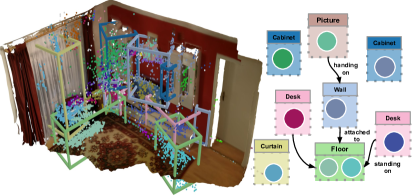
Figure 4: Qualitative evaluation of our scene graph prediction framework. Each 3D bounding box represents a detected entity on the left, and the color is the predicted label. On the right side, we visualize the estimated scene graph on this scene. We only select representative entities on the scene graph visualization for visualization purposes.

Results. Following the evaluation scheme in [64] and in [61], we report two evaluations in Tbl. 1 and Tbl. 2, respectively. The former one maps the node classes to 20 NYUv2 labels [39] to suppress the severe class imbalance in the data as discussed in [62] and estimates a single predicate out of seven support relationship types plus the “same part” relationship to handle over-segmentation. The latter uses 160 node and 26 edge classes with multiple predicate estimation.

In Tbl. 1, overall, it can be seen that all image-based methods (IMP, VGfM, Ours) outperforms points-based methods (3DSSG, SGFN) in almost all object prediction metrics, while the methods based on 3D edge descriptor (3DSSG, SGFN, Ours) tend to have better predicate estimation. This suggests that the 2D representations from images are more representative than 3D, and 3D edge descriptors are more suitable for estimating support types of predicates. By comparing IMP [66] and VGfM [15], it can be seen that the effect of the geometric feature and the temporal message passing is mainly reflected in the mRecall metrics. However, it deteriorates the performance when the input is sparse. A possible reason is that the geometric feature is relatively unstable, which decreases the network performance. It is also reflected in the two 3D methods, i.e. 3DSSG and SGFN, where they failed to perform in classifying objects with sparse segmentation while giving a similar performance in the predicate classification. Among all methods, our method outperforms all baselines among all input types and all metrics, apart from the predicate estimation, which has a slightly worse result on some input types. In addition, we report ours using the proposed incremental estimation pipeline, denoted as Ours(i). The incremental estimation process improves slightly in object estimation. The same behavior is also reported in [64]. We show a qualitative result using our full pipeline in Fig. 4.

In Tbl. 2, our method outperforms all other methods in the relationship and object estimation in Recall and object estimation in mRecall. 3DSSG [61] has the best results in predicate estimations. This suggests that union 3D bounding boxes are more suitable when estimating multiple predicates.

4.3 Incremental Label Association

We evaluate our label association method in the task of incremental entity segmentation, which aims to estimate accurate class-agnostic segmentation given sequential sensor input, with two baseline methods, i.e. InSeg [58] and PanopticFusion [38].

Baseline Methods. Both baseline methods use reference map approaches as mentioned in Sec. 3.1.3. InSeg [58] considers only the overlapping ratio between labels on an estimated mask and a reference mask. PanopticFusion uses IoU [38] as the evaluation method and limits one reference label can only be assigned to one query label.

Implementation. For all methods, we use our IEE pipeline with different label association methods on all training scenes in the 3RScan dataset [60].

Evaluation Metric. We use the Average Overlap Score (AOS) as the evaluation metric [59]. It measures the ratio of the dominant segment of its corresponding ground truth instance. We use the nearest neighbour search to find the ground truth instance label of a reconstructed point. Since our method reconstructs a sparse point map, using the ground truth points as the denominator does not reflect the performance. We instead calculate the score over the sum of all estimated points within the ground truth instance as:

$$\text{AOS}=\sum_{i}\frac{\max_{j}\text{Overlap}(\mathcal{S}_{i},\mathcal{P}_{j})}{\mathbf{\#}\left(\mathcal{S}_{i}\right)},$$ (11)

where $\mathcal{S}_{i}$ is the set of all estimated points with ground truth instance label $i$.

Results. The evaluation result is reported in Tbl. 3. Our approach achieves the highest AOS, which is 1 % higher than InSeg [58] and 3.7% higher than PanopticFusion [38]. The use of a confidence-based approach handles better the label consistency and thus improves the final AOS score. We provide an example of how our method improves temporal consistency under non-uniform distributed points in the supplementary material.

Method	AOS (%)
InSeg [58]	38.6
PanopticFusion [38]	35.9
Ours	39.6

Table 3: Evaluation of different label association methods in the task of incremental entity estimation in 3RScan dataset [60].

4.4 Ablation Study

We ablate our network with two components, i.e. geometric descriptor $\mathbf{g}_{i}$ and relative pose descriptor $R_{i\to j}$. The experiment setup is the same as in [64], which makes the ablation comparable to Tbl. 1. The result is reported in Tbl. 4. More ablation studies are in the supplementary material.

Our vanilla network without $\mathbf{g}_{i}$ and $R_{i\to j}$ outperform baselines in most of the metrics. With $\mathbf{g}_{i}$, there is a consistent improvement on all metrics except the Pred. in mRecall. Compared to VGfM [15] in Tbl. 1, VGfM [15] fails to improve the performance of IMP [66] with sparse input. Our gated geometric feature aggregation improves its baseline with sparse input, bringing a more consistent performance gain than VGfM [15]. The $R_{i\to j}$ improves the mRecall performance with GT and Dense inputs but decreases the model Recall performance. This behavior suggests that $R_{i\to j}$ helps handle class imbalance issues. The combination of both components achieves the best Recall. However, the model tends to focus on dominant classes, resulting in slightly worse performance in mRecall.

	Method		Recall(%)			mRecall
	$\mathbf{g}_{i}$	$R_{i\to j}$	Rel.	Obj.	Pred.	Obj.	Pred.
GT			61.9	76.4	95.6	74.3	69.2
	✓		62.9	77.9	95.9	74.2	64.3
		✓	60.4	76.3	95.0	75.3	73.2
	✓	✓	66.1	81.2	95.6	77.4	71.5
Dense			30.2	54.0	88.5	44.9	33.2
	✓		33.9	56.4	89.7	45.7	33.8
		✓	28.7	52.7	88.2	47.5	34.3
	✓	✓	34.1	58.1	89.9	43.0	33.3
Sparse			9.6	28.6	90.0	25.6	17.7
	✓		9.8	28.5	90.0	25.7	18.1
		✓	9.6	28.1	90.2	23.3	16.9
	✓	✓	9.9	29.5	90.4	23.5	16.5

Table 4: Ablation study on the proposed network. We ablate the proposed gated geometric feature ($\mathbf{g}_{i}$) and the relative pose descriptor ($R_{i\to j}$) using the same experiment setup as in Tbl. 1.

4.5 Runtime

We report the runtime of our system on 3RScan [60] sequence 4acaebcc-6c10-2a2a-858b-29c7e4fb410d in Tbl. 5. The analysis is done with a machine equipped with an Intel Core i7-8700 3.2GHz CPU with 12 threads and a NVidia GeForce RTX 2080ti GPU.

	Front end	Back end
	Sparse Mapping	2D Entity Est.	Label Fusion	Scene Graph Est.
Mean [ms]	14.7	124.6	14.2	52.5

Table 5: Runtime [ms] of the different components of our method.

5 Conclusion

We present a novel method that estimates 3D scene graphs from RGB images incrementally. Our method runs in real-time and does not rely on depth inputs, which could benefit other tasks, such as robotics and AR, that have hardware limitations and real-time demand. The experiment results indicate that our method outperforms others in three different input types. The provided ablation study demonstrates the effectiveness of our design. Our vanilla network, without any geometric input and relative pose descriptor, still outperforms other baselines. Our method provides a novel architecture for estimating scene graphs with only RGB input. The multiview feature is proven to be more powerful than existing 3D methods. Our method can be further improved in many directions. In particular, using semi-direct SLAM methods such as SVO [12] might improve the handling of untextured regions where feature-based methods often fail. In addition, the multiview image encoder could be replaced with a more powerful encoder to improve the scene graph estimation with a computational penalty.

References

- [1] Iro Armeni, Zhi-Yang He, JunYoung Gwak, Amir R Zamir, Martin Fischer, Jitendra Malik, and Silvio Savarese. 3D SceneGgraph: A Structure for Unified Semantics, 3D Space, and Camera. In ICCV, 2019.
- [2] Garrick Brazil, Gerard Pons-Moll, Xiaoming Liu, and Bernt Schiele. Kinematic 3d object detection in monocular video. In European Conference on Computer Vision, pages 135–152. Springer, 2020.
- [3] Carlos Campos, Richard Elvira, Juan J Gómez Rodríguez, José MM Montiel, and Juan D Tardós. Orb-slam3: An accurate open-source library for visual, visual–inertial, and multimap slam. IEEE Transactions on Robotics, 37(6):1874–1890, 2021.
- [4] Nicolas Carion, Francisco Massa, Gabriel Synnaeve, Nicolas Usunier, Alexander Kirillov, and Sergey Zagoruyko. End-to-end object detection with transformers. In European conference on computer vision, pages 213–229. Springer, 2020.
- [5] Chia-Tche Chang, Bastien Gorissen, and Samuel Melchior. Fast oriented bounding box optimization on the rotation group . ACM Trans. Graph., 30(5):122:1–122:16, Oct. 2011.
- [6] Xieyuanli Chen, Andres Milioto, Emanuele Palazzolo, Philippe Giguere, Jens Behley, and Cyrill Stachniss. Suma++: Efficient lidar-based semantic slam. In 2019 IEEE/RSJ International Conference on Intelligent Robots and Systems (IROS), pages 4530–4537. IEEE, 2019.
- [7] Bowen Cheng, Alex Schwing, and Alexander Kirillov. Per-pixel classification is not all you need for semantic segmentation. Advances in Neural Information Processing Systems, 34, 2021.
- [8] Brian Curless and Marc Levoy. A Volumetric Method for Building Complex Models from Range Images. In Proceedings Conference on Computer Graphics and Interactive Techniques, 1996.
- [9] Jia Deng, Wei Dong, Richard Socher, Li-Jia Li, Kai Li, and Li Fei-Fei. Imagenet: A large-scale hierarchical image database. In 2009 IEEE conference on computer vision and pattern recognition, pages 248–255. Ieee, 2009.
- [10] Helisa Dhamo, Azade Farshad, Iro Laina, Nassir Navab, Gregory D Hager, Federico Tombari, and Christian Rupprecht. Semantic Image Manipulation Using Scene Graphs. In CVPR, 2020.
- [11] Helisa Dhamo, Fabian Manhardt, Nassir Navab, and Federico Tombari. Graph-to-3d: End-to-end generation and manipulation of 3d scenes using scene graphs. In Proceedings of the IEEE/CVF International Conference on Computer Vision, pages 16352–16361, 2021.
- [12] Christian Forster, Zichao Zhang, Michael Gassner, Manuel Werlberger, and Davide Scaramuzza. Svo: Semidirect visual odometry for monocular and multicamera systems. IEEE Transactions on Robotics, 33(2):249–265, 2016.
- [13] Sarthak Garg, Helisa Dhamo, Azade Farshad, Sabrina Musatian, Nassir Navab, and Federico Tombari. Unconditional scene graph generation. In Proceedings of the IEEE/CVF International Conference on Computer Vision, pages 16362–16371, 2021.
- [14] Stefano Gasperini, Frithjof Winkelmann, Alvaro Marcos-Ramiro, Micheal Schmidt, Nassir Navab, Benjamin Busam, and Federico Tombari. Holistic segmentation. arXiv preprint arXiv:2209.05407, 2022.
- [15] Paul Gay, James Stuart, and Alessio Del Bue. Visual Graphs from Motion (VGfM): Scene Understanding with Object Geometry Reasoning. In ACCV. Springer, 2018.
- [16] M. Grinvald, F. Furrer, T. Novkovic, J. J. Chung, C. Cadena, R. Siegwart, and J. Nieto. Volumetric Instance-Aware Semantic Mapping and 3D Object Discovery. IEEE Robotics and Automation Letters, 2019.
- [17] Markus Grotz, Peter Kaiser, Eren Erdal Aksoy, Fabian Paus, and Tamim Asfour. Graph-based visual semantic perception for humanoid robots. In 2017 IEEE-RAS 17th International Conference on Humanoid Robotics (Humanoids), pages 869–875. IEEE, 2017.
- [18] Jiuxiang Gu, Shafiq Joty, Jianfei Cai, Handong Zhao, Xu Yang, and Gang Wang. Unpaired image captioning via scene graph alignments. In Proceedings of the IEEE/CVF International Conference on Computer Vision, pages 10323–10332, 2019.
- [19] Jiuxiang Gu, Handong Zhao, Zhe Lin, Sheng Li, Jianfei Cai, and Mingyang Ling. Scene Graph Generation with External Knowledge and Image Reconstruction. In CVPR, 2019.
- [20] Kaiming He, Xiangyu Zhang, Shaoqing Ren, and Jian Sun. Deep residual learning for image recognition. In Proceedings of the IEEE conference on computer vision and pattern recognition, pages 770–778, 2016.
- [21] Mehdi Hosseinzadeh, Yasir Latif, Trung Pham, Niko Suenderhauf, and Ian Reid. Structure aware slam using quadrics and planes. In Asian Conference on Computer Vision, pages 410–426. Springer, 2018.
- [22] Hou-Ning Hu, Qi-Zhi Cai, Dequan Wang, Ji Lin, Min Sun, Philipp Krahenbuhl, Trevor Darrell, and Fisher Yu. Joint monocular 3d vehicle detection and tracking. In Proceedings of the IEEE/CVF International Conference on Computer Vision, pages 5390–5399, 2019.
- [23] N. Hughes, Y. Chang, and L. Carlone. Hydra: A real-time spatial perception system for 3D scene graph construction and optimization. In Robotics: Science and Systems (RSS), 2022.
- [24] Justin Johnson, Agrim Gupta, and Li Fei-Fei. Image Generation from Scene Graphs. In CVPR, 2018.
- [25] KJ Joseph, Salman Khan, Fahad Shahbaz Khan, and Vineeth N Balasubramanian. Towards open world object detection. In Proceedings of the IEEE/CVF Conference on Computer Vision and Pattern Recognition, pages 5830–5840, 2021.
- [26] Andrej Karpathy and Li Fei-Fei. Deep Visual-Semantic Alignments for Generating Image Descriptions. In CVPR, 2015.
- [27] Ue-Hwan Kim, Jin-Man Park, Taek-Jin Song, and Jong-Hwan Kim. 3-d scene graph: A sparse and semantic representation of physical environments for intelligent agents. IEEE transactions on cybernetics, 50(12):4921–4933, 2019.
- [28] Chi Li, Jin Bai, and Gregory D Hager. A unified framework for multi-view multi-class object pose estimation. In Proceedings of the european conference on computer vision (ECCV), pages 254–269, 2018.
- [29] Kejie Li, Daniel DeTone, Yu Fan Steven Chen, Minh Vo, Ian Reid, Hamid Rezatofighi, Chris Sweeney, Julian Straub, and Richard Newcombe. Odam: Object detection, association, and mapping using posed rgb video. In Proceedings of the IEEE/CVF International Conference on Computer Vision, pages 5998–6008, 2021.
- [30] Kejie Li, Hamid Rezatofighi, and Ian Reid. Moltr: Multiple object localization, tracking and reconstruction from monocular rgb videos. IEEE Robotics and Automation Letters, 6(2):3341–3348, 2021.
- [31] Yanwei Li, Hengshuang Zhao, Xiaojuan Qi, Liwei Wang, Zeming Li, Jian Sun, and Jiaya Jia. Fully convolutional networks for panoptic segmentation. In Proceedings of the IEEE/CVF Conference on Computer Vision and Pattern Recognition, pages 214–223, 2021.
- [32] Tsung-Yi Lin, Michael Maire, Serge Belongie, James Hays, Pietro Perona, Deva Ramanan, Piotr Dollár, and C Lawrence Zitnick. Microsoft coco: Common objects in context. In European conference on computer vision, pages 740–755. Springer, 2014.
- [33] Hengyue Liu, Ning Yan, Masood Mortazavi, and Bir Bhanu. Fully convolutional scene graph generation. In Proceedings of the IEEE/CVF Conference on Computer Vision and Pattern Recognition, pages 11546–11556, 2021.
- [34] Cewu Lu, Ranjay Krishna, Michael Bernstein, and Li Fei-Fei. Visual relationship detection with language priors. In European conference on computer vision, pages 852–869. Springer, 2016.
- [35] John McCormac, Ronald Clark, Michael Bloesch, Stefan Leutenegger, and Andrew Davison. Fusion++: Volumetric Object-Level SLAM. In Int. Conf. on 3D Vis., 2018.
- [36] John McCormac, Ankur Handa, Andrew Davison, and Stefan Leutenegger. SemanticFusion: Dense 3D Semantic Mapping with Convolutional Neural Networks. In Int. Conf. Robotics and Automation, 2017.
- [37] Arsalan Mousavian, Dragomir Anguelov, John Flynn, and Jana Kosecka. 3d bounding box estimation using deep learning and geometry. In Proceedings of the IEEE conference on Computer Vision and Pattern Recognition, pages 7074–7082, 2017.
- [38] Gaku Narita, Takashi Seno, Tomoya Ishikawa, and Yohsuke Kaji. PanopticFusion: Online Volumetric Semantic Mapping at the Level of Stuff and Things. In IEEE Conf. Intelligent Robots and Syst., 2019.
- [39] Pushmeet Kohli Nathan Silberman, Derek Hoiem and Rob Fergus. Indoor Segmentation and Support Inference from RGBD Images. In ECCV, 2012.
- [40] Lachlan Nicholson, Michael Milford, and Niko Sünderhauf. Quadricslam: Dual quadrics from object detections as landmarks in object-oriented slam. IEEE Robotics and Automation Letters, 4(1):1–8, 2018.
- [41] Yinyu Nie, Xiaoguang Han, Shihui Guo, Yujian Zheng, Jian Chang, and Jian Jun Zhang. Total3dunderstanding: Joint layout, object pose and mesh reconstruction for indoor scenes from a single image. In Proceedings of the IEEE/CVF Conference on Computer Vision and Pattern Recognition, pages 55–64, 2020.
- [42] Ege Özsoy, Evin Pınar Örnek, Ulrich Eck, Tobias Czempiel, Federico Tombari, and Nassir Navab. 4d-or: Semantic scene graphs for or domain modeling. In International Conference on Medical Image Computing and Computer-Assisted Intervention. Springer, 2022.
- [43] Ege Özsoy, Evin Pınar Örnek, Ulrich Eck, Federico Tombari, and Nassir Navab. Multimodal semantic scene graphs for holistic modeling of surgical procedures. In Arxiv, 2021.
- [44] Quang-Hieu Pham, Binh-Son Hua, Thanh Nguyen, and Sai-Kit Yeung. Real-time Progressive 3D Semantic Segmentation for Indoor Scene. In IEEE Winter Conf. Appli. Comput. Vis., 2019.
- [45] Charles Ruizhongtai Qi, Hao Su, Kaichun Mo, and Leonidas Guibas. PointNet: Deep Learning on Point Sets for 3D Classification and Segmentation. In CVPR, 2017.
- [46] Lu Qi, Jason Kuen, Yi Wang, Jiuxiang Gu, Hengshuang Zhao, Zhe Lin, Philip Torr, and Jiaya Jia. Open-world entity segmentation. arXiv preprint arXiv:2107.14228, 2021.
- [47] Zachary Ravichandran, Lisa Peng, Nathan Hughes, J Daniel Griffith, and Luca Carlone. Hierarchical representations and explicit memory: Learning effective navigation policies on 3d scene graphs using graph neural networks. In 2022 International Conference on Robotics and Automation (ICRA), pages 9272–9279. IEEE, 2022.
- [48] Antoni Rosinol, Arjun Gupta, Marcus Abate, Jingnan Shi, and Luca Carlone. 3D Dynamic Scene Graphs: Actionable Spatial Perception with Places, Objects, and Humans. Comput. Res. Repository, 2020.
- [49] Antoni Rosinol, Arjun Gupta, Marcus Abate, Jingnan Shi, and Luca Carlone. 3d dynamic scene graphs: Actionable spatial perception with places, objects, and humans. arXiv preprint arXiv:2002.06289, 2020.
- [50] Antoni Rosinol, Andrew Violette, Marcus Abate, Nathan Hughes, Yun Chang, Jingnan Shi, Arjun Gupta, and Luca Carlone. Kimera: From slam to spatial perception with 3d dynamic scene graphs. The International Journal of Robotics Research, 40(12-14):1510–1546, 2021.
- [51] Martin Runz, Maud Buffier, and Lourdes Agapito. Maskfusion: Real-time recognition, tracking and reconstruction of multiple moving objects. In 2018 IEEE International Symposium on Mixed and Augmented Reality (ISMAR), pages 10–20. IEEE, 2018.
- [52] Radu Bogdan Rusu and Steve Cousins. 3D is here: Point Cloud Library (PCL). In IEEE International Conference on Robotics and Automation (ICRA), Shanghai, China, May 9-13 2011.
- [53] Renato F. Salas-Moreno, Richard A. Newcombe, Hauke Strasdat, Paul H. J. Kelly, and Andrew J. Davison. SLAM++: Simultaneous Localisation and Mapping at the Level of Objects. In CVPR, 2013.
- [54] Raluca Scona, Simona Nobili, Yvan R Petillot, and Maurice Fallon. Direct visual slam fusing proprioception for a humanoid robot. In 2017 IEEE/RSJ International Conference on Intelligent Robots and Systems (IROS), pages 1419–1426. IEEE, 2017.
- [55] Philipp Seiwald, Shun-Cheng Wu, Felix Sygulla, Tobias FC Berninger, Nora-Sophie Staufenberg, Moritz F Sattler, Nicolas Neuburger, Daniel Rixen, and Federico Tombari. Lola v1. 1–an upgrade in hardware and software design for dynamic multi-contact locomotion. In 2020 IEEE-RAS 20th International Conference on Humanoid Robots (Humanoids), pages 9–16. IEEE, 2021.
- [56] Olivier Stasse, Andrew J Davison, Ramzi Sellaouti, and Kazuhito Yokoi. Real-time 3d slam for humanoid robot considering pattern generator information. In 2006 IEEE/RSJ International Conference on Intelligent Robots and Systems, pages 348–355. IEEE, 2006.
- [57] Hang Su, Subhransu Maji, Evangelos Kalogerakis, and Erik Learned-Miller. Multi-view convolutional neural networks for 3d shape recognition. In Proceedings of the IEEE international conference on computer vision, pages 945–953, 2015.
- [58] Keisuke Tateno, Federico Tombari, and Nassir Navab. Real-Time and Scalable Incremental Segmentation on Dense SLAM. In IEEE Conf. Intelligent Robots and Syst., 2015.
- [59] Keisuke Tateno, Federico Tombari, and Nassir Navab. Large scale and long standing simultaneous reconstruction and segmentation. Computer Vision and Image Understanding, 157:138–150, 2017.
- [60] Johanna Wald, Armen Avetisyan, Nassir Navab, Federico Tombari, and Matthias Nießner. RIO: 3D Object Instance Re-Localization in Changing Indoor Environments. In ICCV, 2019.
- [61] Johanna Wald, Helisa Dhamo, Nassir Navab, and Federico Tombari. Learning 3D Semantic Scene Graphs from 3D Indoor Reconstructions. In CVPR, 2020.
- [62] Johanna Wald, Nassir Navab, and Federico Tombari. Learning 3d semantic scene graphs with instance embeddings. International Journal of Computer Vision, pages 1–22, 2022.
- [63] Xin Wei, Yifei Gong, Fudong Wang, Xing Sun, and Jian Sun. Learning canonical view representation for 3d shape recognition with arbitrary views. In Proceedings of the IEEE/CVF International Conference on Computer Vision, pages 407–416, 2021.
- [64] Shun-Cheng Wu, Johanna Wald, Keisuke Tateno, Nassir Navab, and Federico Tombari. Scenegraphfusion: Incremental 3d scene graph prediction from rgb-d sequences. In Proceedings of the IEEE/CVF Conference on Computer Vision and Pattern Recognition, pages 7515–7525, 2021.
- [65] Yanmin Wu, Yunzhou Zhang, Delong Zhu, Yonghui Feng, Sonya Coleman, and Dermot Kerr. Eao-slam: Monocular semi-dense object slam based on ensemble data association. In 2020 IEEE/RSJ International Conference on Intelligent Robots and Systems (IROS), pages 4966–4973. IEEE, 2020.
- [66] Danfei Xu, Yuke Zhu, Christopher Choy, and Li Fei-Fei. Scene Graph Generation by Iterative Message Passing. In CVPR, 2017.
- [67] Kelvin Xu, Jimmy Ba, Ryan Kiros, Kyunghyun Cho, Aaron Courville, Ruslan Salakhudinov, Rich Zemel, and Yoshua Bengio. Show, Attend and Tell: Neural Image Caption Generation with Visual Attention. In Int. Conf. Mach. Learn., 2015.
- [68] Jianwei Yang, Jiasen Lu, Stefan Lee, Dhruv Batra, and Devi Parikh. Graph R-CNN for Scene Graph Generation. In ECCV, 2018.
- [69] Shichao Yang and Sebastian Scherer. Cubeslam: Monocular 3-d object slam. IEEE Transactions on Robotics, 35(4):925–938, 2019.
- [70] Cheng Zhang, Zhaopeng Cui, Yinda Zhang, Bing Zeng, Marc Pollefeys, and Shuaicheng Liu. Holistic 3d scene understanding from a single image with implicit representation. In Proceedings of the IEEE/CVF Conference on Computer Vision and Pattern Recognition, pages 8833–8842, 2021.
- [71] Jiazhao Zhang, Chenyang Zhu, Lintao Zheng, and Kai Xu. Fusion-Aware Point Convolution for Online Semantic 3D Scene Segmentation. In CVPR, 2020.
- [72] Yiwu Zhong, Jing Shi, Jianwei Yang, Chenliang Xu, and Yin Li. Learning to generate scene graph from natural language supervision. In Proceedings of the IEEE/CVF International Conference on Computer Vision, pages 1823–1834, 2021.