Collective Lamb Shift and Spontaneous Emission of A Dense Atomic Gas

Abstract

Finding a comprehensive and general description of the collective Lamb shift and cooperative broadening in a radiatively interacting system is a long-standing open question. Both, energy levels and decay rates, are modified by the exchange of real and virtual photons making up the dipole-dipole interaction. We introduce a method to theoretically study weakly-driven, low-excited ensembles of two-level atoms and obtain an analytic description of the collective Lamb shift and collective decay rate via a self-consistent formalism including multiple scattering. We predict the dependency of these quantities, as measurables, on system parameters: the number density of the ensemble, the detuning of an external probe field, and the geometry of the sample.

Ensembles of radiators can manifest collective effects as a consequence of dipole-dipole interactions mediated by photons. These effects can alter the radiative properties, including the buildup of collective modes called superradiance and subradiance with enhanced or suppressed decay rates [1, 2], as well as the shift of transition frequency [3]. The collective Lamb shift [4, 5], which results from the exchange of virtual photons between radiators, has attracted much attention in both theoretical discussions and experimental studies [6, 7, 8]. In the case of single excitation, the shift can be found by diagonalizing the equations of motion [9, 10, 11]. Meanwhile, classical electrodynamics simulations are also used to study spatially extended systems [12, 13, 14]. Experimental observations of collective Lamb shift have been reported in solid state samples [15], atomic arrays [16] and atomic gas [17, 18, 19, 20, 21, 22, 23]. However, the counterpart of the collective shift – the modification of spontaneous decay – lacks investigation so far. In most discussions to date, the effects of the modified modes [24, 25, 26] and the effects of re-absorption and re-emission of coherent and incoherent photons are not differentiated. In order to understand the collective Lamb shift, however, one has to concentrate on cooperative phenomena interacting only with the vacuum field. The Lamb shift and the spontaneous decay rate of a collective system, as they are profoundly connected via the Green’s function, need to be studied simultaneously.

In this Letter, we develop a self-consistent relation that analytically describes the collective Lamb shift and the collective spontaneous decay rate of a dense ensemble. This relation is governed by the local number density of atoms and the detuning of the external probe field. The scheme to derive such a relation can be summarized as follows: First, a master equation for two probe atoms (Fig. 1 (a)) is derived under the Markov approximation. The modified decay rates and level shifts of the probe atoms can be obtained by the real and imaginary parts of a dressed Green’s function that describes the emission and re-absorption of real and virtual photons between probe and background atoms (Fig. 1 (b)). Second, the dressed Green’s function is calculated via the Dyson equation [27], and is expressed in terms of averaged two-point correlators of atomic operators. Third, by virtue of the quantum regression theorem [28], the averaged two-point atomic correlators are treated self-consistently and take into account multiple scattering to infinite order. This leads, finally, to a closed form of the modified decay rates and level shifts for a steady state. To predict measurable effects in experiments, one needs to take into account the geometry of the sample and average over the distribution of probe atoms. The mathematical background to this treatment can be found in Refs. [29, 30].

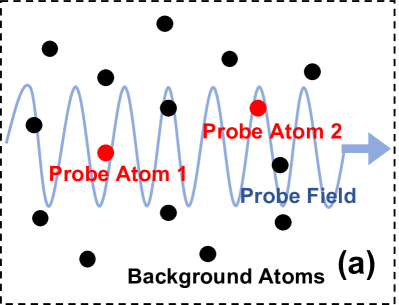
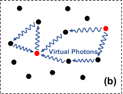
Figure 1: (a) A pictorial demonstration of the atomic gas driven by an external probe field. The reduced density matrix includes two arbitrarily chosen probe-atoms, while all other atoms as well as the field are traced out. (b) The emission and reabsorption of virtual photons result in the modifications of Lamb shift and spontaneous decay rate.

In order to understand the dynamics, we consider an ensemble of identical two-level atoms that interact with the electric field, with the full Hamiltonian

$$H=\sum_{i=1}^{N}\hbar\omega_{0}\sigma^{\dagger}_{i}\sigma_{i}+\sum_{\vec{k},\lambda}\hbar\omega_{l}(\vec{k})a^{\dagger}_{\vec{k},\lambda}a_{\vec{k},\lambda}-\sum_{i=1}^{N}\vec{p}_{i}\cdot(\vec{\cal E}_{i}+\vec{E}_{i})$$ (1)

where $\sigma^{\dagger}_{i}=\left|e_{i}\right\rangle\!\!\left\langle g_{i}\right|$ and $\sigma_{i}=\left|g_{i}\right\rangle\!\!\left\langle e_{i}\right|$ are the raising and lowering operators of the $i$-th atom, $a^{\dagger}$ and $a$ are the creation and annihilation operators of the photons. We assume that the atoms mostly couple to the field modes with frequencies $\omega_{l}$ that are close to the atomic resonant frequency $\omega_{0}$. $\vec{p}_{i}=\hat{\epsilon}_{i}\wp(\sigma_{i}+\sigma_{i}^{\dagger})$ is the dipole operator of the $i$-th atom with dipole matrix element $\wp$. $\vec{\cal E}_{i}$ is the external classical driving field, while $\vec{E}_{i}$ is the quantized field operator, at the position of the $i$-th atom. Here, we focus on the dynamics of two arbitrarily chosen probe atoms, and formally trace out the quantized field and the rest $N-2$ atoms [28, 31]. A Lindblad form master equation with rotating-wave approximation in the rotating frame is obtained for the two probe-atoms [30]

$$\dot{\rho} = -\frac{i}{\hbar}[\tilde{H}_{0},\rho]+i\Omega\sum_{i=1,2}[\sigma_{i}+\sigma_{i}^{\dagger},\rho]-i\sum_{i,j=1,2}\delta_{ij}[\sigma^{\dagger}_{j}\sigma_{i},\rho]$$ (2)

$$-\sum_{i,j=1,2}\frac{\gamma_{ij}}{2}(\sigma_{j}^{\dagger}\sigma_{i}\rho-2\sigma_{i}\rho\sigma_{j}^{\dagger}+\rho\sigma_{j}^{\dagger}\sigma_{i})$$

where $\tilde{H}_{0}=\hbar(\omega_{0}-\omega_{c})\sum_{i}\sigma^{\dagger}_{i}\sigma_{i}=\hbar\Delta_{0}\sum_{i}\sigma^{\dagger}_{i}\sigma_{i}$ is the two-atom free Hamiltonian in the rotating frame, with a classical driving frequency $\omega_{c}$. $\Omega=|\wp{\cal E}_{0}/\hbar|$ is the Rabi frequency, with the driving amplitude ${\cal E}_{0}$. Note that a positive $\Delta_{0}$ stands for a red-detuned driving field. The two sets of parameters, $\gamma_{ij}$ and $\delta_{ij}$, describe the modified spontaneous decay rate and the collective Lamb shift respectively. It is commonly accepted that for atoms placed in free-space, $\gamma_{ij}$ and $\delta_{ij}$ are associated with the free-space Green’s tensor that results from the dipole-dipole interaction, written as a function of distance between two spatial points [32, 24, 25, 26]

$$G^{(0)}_{\alpha\beta}(r,\omega) = -\frac{i\hbar e^{-i\omega r/c}}{4\pi\epsilon_{0}r}\bigg{[}\delta_{\alpha\beta}\bigg{(}\frac{\omega^{2}}{c^{2}}-i\frac{\omega}{c}\frac{1}{r}-\frac{1}{r^{2}}\bigg{)}$$ (3)

$$+\frac{x_{\alpha}x_{\beta}}{r^{2}}\bigg{(}-\frac{\omega^{2}}{c^{2}}+3i\frac{\omega}{c}\frac{1}{r}+\frac{3}{r^{2}}\bigg{)}\bigg{]}$$

The decay rate and frequency shift in the master equation are then $\gamma_{ij}\!\!\sim\!\!{\rm Re}[G^{(0)}]$ and $\delta_{ij}\!\!\sim\!\!{\rm Im}[G^{(0)}]$. However, these relations are no longer correct in a dense system, since one has to consider the multiple scattering of virtual photons between the particles (Fig. 1 (b)). Therefore, a complete Green’s function should be the free-space term in Eq. (3) plus all orders of corrections that describe the multiple scattering. The modified decay rate $\gamma_{ij}$ and collective Lamb shift $\delta_{ij}$ will therefore connect to a dressed Green’s function.

The dressed Green’s function can be found via the formal expressions for $\gamma_{ij}$ and $\delta_{ij}$, which can be obtained by tracing out the background atoms and the quantized field [33]. They are related to the Fourier transform of the quantized field correlators as follows [29, 30]

$$\gamma_{ij}(t)= \frac{\wp^{2}}{\hbar^{2}}\int_{-\infty}^{+\infty}\langle[E_{j}^{+}(t),E_{i}^{-}(t+\tau)]\rangle e^{-i(\omega_{0}-\omega_{l})\tau}d\tau$$ (4a)

$$\delta_{ij}(t)= -\frac{i\wp^{2}}{2\hbar^{2}}\int_{0}^{+\infty}\langle[E_{j}^{+}(t+\tau),E_{i}^{-}(t)]\rangle e^{i(\omega_{0}-\omega_{l})\tau}d\tau$$

$$+\frac{i\wp^{2}}{2\hbar^{2}}\int_{0}^{+\infty}\langle[E_{j}^{+}(t),E_{i}^{-}(t+\tau)]\rangle e^{-i(\omega_{0}-\omega_{l})\tau}d\tau$$ (4b)

where $E_{i}^{+}$($E_{i}^{-}$) is the positive (negative) frequency component of the field operator in Heisenberg picture. One can reproduce the free-space spontaneous decay rate and Lamb shift by using the free-field operators in Eq. (4) [29]. For two arbitrarily chosen probe atoms, Eq. (2) is effectively averaged over all possible choices of atomic pairs, thus a permutational symmetry is imposed such that $\gamma_{11}=\gamma_{22}$, $\gamma_{12}=\gamma_{21}$, and similarly for $\delta_{ij}$. A Comprehensive derivation of Eqs. (2) and (4) for a dense atomic gas can be found in Ref. [30], where the authors also take into account the contribution to the decay rate and frequency shift which scales with the number of photons. Here, we consider a low-excited gas and neglect those effects.

We define the dressed Green’s function in the medium as

$$D_{ij}(\tau,t)=D(\vec{r}_{i},t+\tau,\vec{r}_{j},t)=\theta(\tau)\langle[E^{-}_{i}(t+\tau),E^{+}_{j}(t)]\rangle$$ (5)

and its Fourier transform with respect to $\tau$, $\tilde{D}_{ij}(\omega,t)=\int_{-\infty}^{+\infty}D_{ij}(\tau,t)e^{-i\omega\tau}d\tau$, where $\theta(\tau)$ is the Heaviside step function. In medium, $D_{ij}$ obeys a general form of Dyson equation [27, 29]

$$D(\vec{r}_{i},t_{i},\vec{r}_{j},t_{j})=D^{(0)}(\vec{r}_{i},t_{i},\vec{r}_{j},t_{j})-\int\!dt_{k}\!\int\!dt_{l}\!\int\!d^{3}\!r_{k}$$

$$\times D^{(0)}(\vec{r}_{i},t_{i},\vec{r}_{k},t_{k})P(\vec{r}_{k},t_{k},t_{l})D(\vec{r}_{k},t_{l},\vec{r}_{j},t_{j})$$ (6)

where $D^{(0)}$ is the scalar free-space Green’s function. In frequency space, $\tilde{D}^{(0)}$ can be obtained from Eq. (3) by averaging over random polarization and replacing $x_{\alpha}x_{\beta}/r^{2}\!\!\to\!\!\delta_{\alpha\beta}/3$, with the form

$$\tilde{D}_{ij}^{(0)}(\omega,t)=-\frac{i\hbar\omega_{0}^{2}}{6\pi\epsilon_{0}c^{2}r}e^{-i\omega_{0}r/c}$$ (7)

The source function $P$ has the following form in a continuum approximation

$$P(\vec{r}_{i},t_{1},t_{2})=\frac{\wp^{2}{\cal N}}{\hbar^{2}}\theta(t_{1}-t_{2})\langle[\sigma^{\dagger}_{i}(t_{1}),\sigma_{i}(t_{2})]\rangle$$ (8)

where ${\cal N}$ is the number density of the radiators. By iteration, the second term in Eq. (Collective Lamb Shift and Spontaneous Emission of A Dense Atomic Gas) includes a sum of all orders in $P$, describing multiple scattering of photons to all orders. The correlation function on the right hand side of Eq. (8) can be further expressed in terms of the elements of the density matrix by using the quantum regression theorem [33].

In Ref. [29, 30], we solve Eq. (Collective Lamb Shift and Spontaneous Emission of A Dense Atomic Gas) in Fourier space for $\tilde{D}_{ij}$ for a gas of randomly polarized radiators:

$$\tilde{D}_{ij}(\omega,t)=-\frac{i\hbar\omega_{0}^{2}}{6\pi\epsilon_{0}c^{2}r}{\rm exp}\bigg{(}-i\frac{\omega_{0}r}{c}\sqrt{1+\frac{2i\hbar}{3\epsilon_{0}}\tilde{P}(\omega,t)}\bigg{)}$$ (9)

where $r=|\vec{r}_{i}-\vec{r}_{j}|$ is the distance between the radiators. Here, the source function $\tilde{P}$ takes a spatial average and is independent of the location. Note that by setting $\tilde{P}=0$, Eq. (9) reduces to Eq. (7) in the randomly polarized condition, so the Green’s function is indeed dressed by the source function $\tilde{P}$.

We further assume weak-driving and low-excitation conditions in the sample. This approximation is valid, for example, in a weakly driven atomic gas [18, 23]. We will approach the limit $\Omega\to 0$ in the expression of $\tilde{P}$. The Fourier variable in Eq. (9) takes the value $\omega=\omega_{0}-\omega_{l}\approx\delta_{11}$. The source function is then simplified to [33]

$$\tilde{P}(\omega\approx\delta_{11},t)=\frac{\wp^{2}}{\hbar^{2}}{\cal N}\frac{-2}{\gamma_{11}-2i\Delta_{0}}$$ (10)

which depends on the density of radiators, the modified single-atom decay rate and the detuning of the driving field.

Using the definition in Eq. (5), we find Eq. (4) becomes the real and imaginary parts of the dressed Green’s functions.

$$\gamma_{ij} =-2\frac{\wp^{2}}{\hbar^{2}}{\rm Re}\big{(}\tilde{D}_{ij}\big{)}$$ (11a)

$$\delta_{ij} =\frac{\wp^{2}}{\hbar^{2}}{\rm Im}\big{(}\tilde{D}_{ij}\big{)}$$ (11b)

For simplicity, we define the effective wave number $q_{0}$

$$q_{0}=q_{0}^{\prime}+iq_{0}^{\prime\prime}=\frac{\omega_{0}}{c}\sqrt{1+\frac{2i\hbar}{3\epsilon_{0}}\tilde{P}}$$ (12)

By taking the limit $r\to 0$, the single-atom spontaneous decay rate is associated with the real part of the effective wave number $q_{0}$.

$$\gamma_{ii}=\gamma_{ij}(r\to 0)=-2\frac{\wp^{2}}{\hbar^{2}}\lim_{r\to 0}{\rm Re}\big{(}\tilde{D}_{ij}\big{)}=\gamma_{0}\frac{\lambda}{2\pi}q_{0}^{\prime}$$ (13)

where $\lambda=2\pi c/\omega_{0}$ is the wavelength of the transition, and $\gamma_{0}=\wp^{2}\omega^{3}_{0}/3\pi\hbar\epsilon_{0}c^{3}$ is the free-space spontaneous decay rate. For the Lamb shift, we renormalize to the vacuum value:

$$\delta_{ii}^{\prime} = \delta_{ij}(r\to 0)-\delta_{ij}^{(0)}(r\to 0)$$ (14)

$$= \frac{\wp^{2}}{\hbar^{2}}\lim_{r\to 0}{\rm Im}\big{(}\tilde{D}_{ij}-\tilde{D}^{(0)}_{ij}\big{)}=-\gamma_{0}\frac{\lambda}{4\pi}q_{0}^{\prime\prime}$$

By substituting Eq. (13) and Eq. (14) to Eq. (12) and making use of the form in Eq. (10), one can obtain a self-consistent relation for the self-energy terms $\gamma_{ii}$ and $\delta_{ii}^{\prime}$

$$1+\frac{2C}{2\frac{\Delta_{0}}{\gamma_{0}}+i\frac{\gamma_{ii}}{\gamma_{0}}}=\bigg{(}\frac{\gamma_{ii}}{\gamma_{0}}-i\frac{2\delta_{ii}^{\prime}}{\gamma_{0}}\bigg{)}^{2}$$ (15)

where we have defined the cooperativity parameter $C=\frac{\lambda^{3}{\cal N}}{4\pi^{2}}$ which is proportional to the number density. Eq. (15) is the first main result of this paper. In an ensemble of radiators, both the spontaneous decay rate and the Lamb shift of an individual atom are modified due to the collective nature of the dynamics. Under the weak-driving and low-excitation conditions, both quantities together satisfy Eq. (15) which is governed by the density of the radiators ($C$) and the detuning of the driving ($\Delta_{0}$).

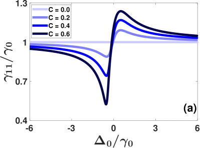
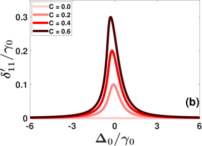
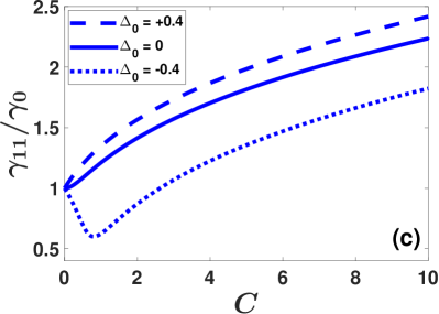
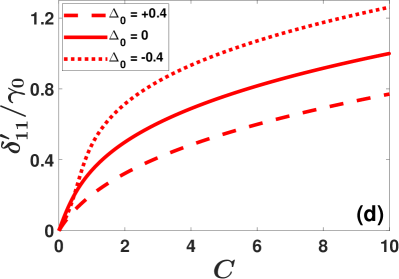
Figure 2: (a) The single-atom spontaneous decay rate modified by the collective effect, in units of the free-space decay rate $\gamma_{0}$. The value changes with respect to the detuning of the external driving field ($\Delta_{0}$), and the number density of emitters ($C$). (b) The single-atom Lamb shift modified by the collective effect, as a function of detuning. (c) The single-atom spontaneous decay rate as a function of particle density, with three different detunings. (d) The single-atom Lamb shift as a function of particle density.

Fig. 2 shows the solution of Eq. (15), which has a modified Lorentzian profile. By varying the detuning of the external driving field and the density of particles, one can tune both the modified decay rate and the Lamb shift. At low-density or in far-detuned regions, both quantities recover the free-space values, namely, $\gamma_{11}\to\gamma_{0}$ and $\delta_{11}^{\prime}\to 0$. As the particle density gets higher, the collective effect predominates and leads to modification of both quantities. It is clear to see from Fig. 2(a) that a red-detuned driving field leads to an enhancement of spontaneous emission, while a blue-detuned driving field results in a suppression. A positive $\delta_{11}^{\prime}$ stands for a red shift of radiated light in our definition.

In Fig. 2(c,d) we plot the decay rate and the Lamb shift as functions of particle density, with different external detunings. Here, the parameter $C=1$, for example, corresponds to $\sim\!40$ particles contained in a cubed wavelength, which is $\sim\!8\times 10^{13}/cm^{3}$ for Rb 780 nm transition. The minimum of $\gamma_{11}$ around $C=0.8$ corresponds to the valley at the blue-detuned region in Fig. 2(a). In the low density region ($C<0.5$), the Lamb shift increases linearly, while for high density, it exhibits sub-linear behavior.

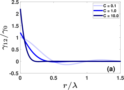
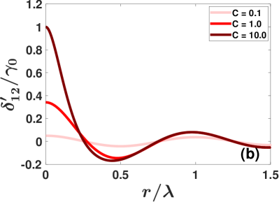
Figure 3: The two-atom terms of (a) modified decay rate and (b) Lamb shift as functions of distance between the two particles ($r$) in units of transition wavelength, with different particle density ($C$). In both calculations the driving is on-resonant with $\Delta_{0}=0$.

The two-atom terms $\gamma_{12}$ and $\delta_{12}$ can be calculated from Eq. (11) as functions of inter-atom distance, and are shown in Fig. 3. An oscillatory behavior is shown, which results from the constructive/destructive contributions from the paired atom. At small $r$ limit both quantities reduce to the single-atom values, while at large $r$ limit both vanish.

This finally leads to expressions for measurable decay rate $\gamma$ and collective Lamb shift $\delta$. For a weak driving, the $\Omega$ term in Eq. (2) can be treated as a perturbation, which leads to the following steady-state equations in the first order of $\Omega$

$$0\!= -\bigg{[}\frac{\gamma_{11}}{2}+i(\delta_{11}+\Delta_{0})\bigg{]}\rho_{eg}\!+\!\big{(}\frac{\gamma_{12}}{2}+i\delta_{12}\big{)}m_{eg}+i\Omega$$ (16a)

$$0\!= -\bigg{[}\frac{3}{2}\gamma_{11}\!+\!\gamma_{12}\!+\!i(\delta_{11}\!+\!\Delta_{0})\bigg{]}m_{eg}$$

$$-\!\big{(}\gamma_{11}\!+\!\frac{\gamma_{12}}{2}\!-\!i\delta_{12}\big{)}\rho_{eg}-i\Omega$$ (16b)

where $\rho_{eg}=\frac{1}{2}(\langle\sigma_{1}\rangle+\langle\sigma_{2}\rangle)$ is the average single-atom coherence, and $m_{eg}$ is defined as $m_{eg}=\frac{1}{2}(\langle\sigma_{1}\sigma_{z2}\rangle+\langle\sigma_{z1}\sigma_{2}\rangle)$. The solution is

$$\rho_{eg} = \frac{\Omega}{\delta_{11}+\delta_{12}+\Delta_{0}-i\frac{\gamma_{11}+\gamma_{12}}{2}}$$ (17)

$$m_{eg} = -\rho_{eg}$$ (18)

Therefore, the effective single-atom density matrix in the weak-driving, low-excited condition has the following form:

$$\rho^{\rm eff}=\begin{pmatrix}0&\rho^{\rm eff}_{eg}\\ \rho^{\rm eff}_{ge}&1\end{pmatrix}$$ (19)

where $\rho^{\rm eff}_{eg}$ is the average over all possible choices of probe atom pairs, with a particular particle distribution $f(\vec{r})$.

$$\rho^{\rm eff}_{eg} = \int\!\!\!\!\int d^{3}r_{1}d^{3}r_{2}f(\vec{r}_{1})f(\vec{r}_{2})$$ (20)

$$\times\frac{\Omega}{\delta_{11}+\delta_{12}(r)+\Delta_{0}-i\frac{\gamma_{11}+\gamma_{12}(r)}{2}}$$

where $r=|\vec{r}_{1}-\vec{r}_{2}|$. One can further define the effective decay rate $\gamma^{\rm eff}$ and the effective collective Lamb shift $\delta^{\rm eff}$ for a given sample by

$$\rho^{\rm eff}_{eg}=\frac{\delta^{\rm eff}+i\frac{\gamma^{\rm eff}}{2}}{(\delta^{\rm eff})^{2}+(\frac{\gamma^{\rm eff}}{2})^{2}}\Omega$$ (21)

$\gamma^{\rm eff}$ and $\delta^{\rm eff}$ are the quantities that can be measured in experiments.

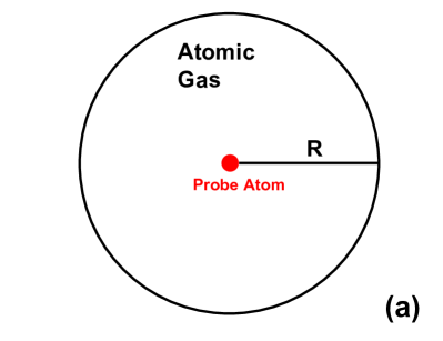
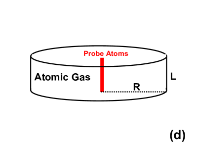
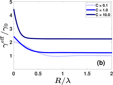
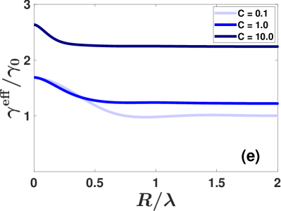
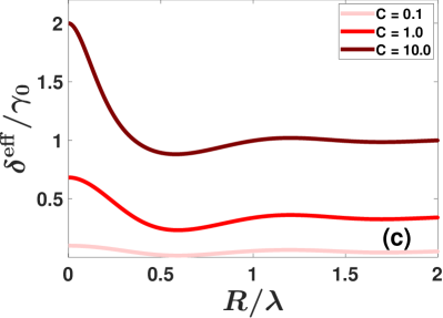
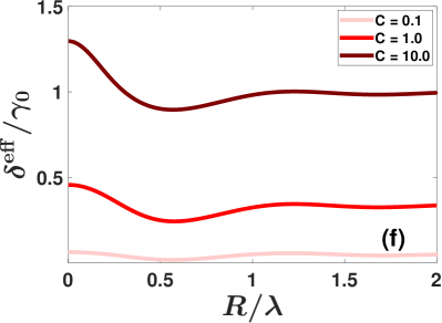
Figure 4: (a) A pictorial demonstration of a spherical cloud of radiators, with radius $R$. The probe atom is considered to be at the center, while the second atom has been averaged over the volume. (b) The effective decay rate of the central atom of a spherical cloud, as a function of the radius of the cloud, plotted with different particle densities. (c) The effective Lamb shift of the central atom of a spherical cloud. (d) A pictorial demonstration of a cylindrical cloud of radiators, with varying radius $R$ and fixed thickness $L=0.5\lambda$. The probe atom is averaged over central axis of the cylinder. (e) The effective decay rate of the central atoms of a cylindrical gas, as a function of the radius, plotted with different particle densities. (f) The effective Lamb shift of the central atoms of a cylindrical gas.

As an example, we consider a spherical cloud of radiators with uniform distribution $f(\vec{r})=\frac{1}{V}$ and radius $R$ (Fig. 4 (a)). For simplicity, we study the effective decay rate and collective Lamb shift of a probe atom located at the center of the sphere, namely, the integrations in Eq. (20) is taken only once for the second atom over the volume. The result is shown in Fig. 4 (b,c), where the effective, collective spontaneous decay and the Lamb shift of the center atom are plotted as functions of the radius of the sphere, with different cooperativity parameter $C$. By and large, both $\gamma^{\rm eff}$ and $\delta^{\rm eff}$ decrease with larger radius of the atomic gas. As $R\to\infty$, both quantities asymptotically approach the single-atom terms $\gamma_{11}$ and $\delta_{11}$, which are the homogeneous limits for an infinite size ensemble. The effective collective Lamb shift shows a great oscillation in small $R$, with sufficiently high particle density. The minimum of $\delta^{\rm eff}$ (least red shift) is found when the radius is near half of the transition wavelength.

Similarly, a numeric result for a cylinder-shaped gas is shown in Fig. 4 (e,f), where the thickness of the gas is fixed to $0.5\lambda$, and the modified decay rate and Lamb shift are plotted as functions of the radius. In this case, the second atom is averaged over the whole volume, while the first atom is averaged over the central axis of the cylinder. For large radius $R$, this resembles an infinitely extended slab that is a commonly adopted condition in recent experiments [18, 23].

In conclusion, we have developed a theoretical framework to describe the collective radiation of dense ensembles. In particular, a weakly driven – low-excited condition is imposed, and the collective modification of Lamb shift and spontaneous emission rate are studied both analytically and numerically. We find that these quantities are connected via a dressed Green’s function that describes the exchange and multiple scattering of real and virtual photons in the medium. The dressed Green’s function, together with the master equation, lead to a self-consistent relation of decay rate and Lamb shift that shows their dependencies on the density of radiators and the detuning of the probe field. The decay rate and collective Lamb shift have a modified Lorentzian profile with respect to the detuning of the probe field, and the modification scales with the particle density. We find both enhancement and suppression of the decay rate, and an overall red-shift of the collective Lamb shift. We numerically predict the averaged effects that can be measured by experiments, and find oscillatory behavior as the size of the sample changes. These effects are at the order of the vacuum decay rate $\gamma_{0}$, and are already noticeable for a density low as $\sim\!8\times 10^{13}/cm^{3}$ for Rb 780nm transition. Our work provides insights into the collective effects of radiative systems and is instructive to future experiments.

We thank Stefan Ostermann and Oriol Rubies-Bigorda for helpful discussions. We would like to thank the NSF for funding through PHY-1912607 and PHY-2207972 and the AFOSR through FA9550-19-1- 0233.

I Supplemental Material

I.1 I. Derivation of $\gamma_{ij}$ and $\delta_{ij}$

Here, We outline the derivation of the two-atom master equation and read off the expressions of $\gamma_{ij}$ and $\delta_{ij}$. Details of the derivation is given in Ref. [30]. The full Hamiltonian can be separated into two parts

$$H = \sum_{i=1}^{N}\hbar\omega_{0}\sigma^{\dagger}_{i}\sigma_{i}+\sum_{\vec{k},\lambda}\hbar\omega_{l}(\vec{k})a^{\dagger}_{\vec{k},\lambda}a_{\vec{k},\lambda}-\sum_{i\neq 1,2}\vec{p}_{i}\cdot(\vec{\cal E}_{i}+\vec{E}_{i})-\sum_{i=1,2}\vec{p}_{i}\cdot(\vec{\cal E}_{i}+\vec{E}_{i})$$ (22)

$$= H_{0}+V$$ (23)

where $V=-\sum_{i=1,2}\vec{p}_{i}\cdot(\vec{\cal E}_{i}+\vec{E}_{i})$ only contains two probe atoms. We implement the Keldysh formalism and define the effective two-atom time-evolution operator along the Keldysh contour

$${\cal S}^{\rm eff}_{\cal C}\equiv\langle{\cal S}_{\cal C}\rangle_{E}=\left\langle{\cal T}_{\cal C}{\rm exp}\left\{-\frac{i}{\hbar}\int_{\cal C}d\check{\tau}V^{I}(\check{\tau})\right\}\right\rangle_{E}$$ (24)

where $\langle...\rangle_{E}={\rm Tr}_{E}(...\rho_{E})$ denotes an average over the environmental degrees of freedom, namely, the $N-2$ atoms and the quantized field. $V^{I}(t)=e^{iH_{0}(t-t_{0})/\hbar}Ve^{-iH_{0}(t-t_{0})/\hbar}$ is the $V$ term in the interaction picture. $\cal C$ represents an integration path from $-\infty$ to $t$, then from $t$ to $-\infty$, with ${\cal T}_{\cal C}$ being the normal time-ordering for the first part and the inverse time-ordering for the second. The matrix element of the density matrix can be written as the expectation value of the corresponding projection operator.

$$\rho_{\alpha\beta}(t)=\langle{\cal T}_{\cal C}{\cal S}^{\rm eff}_{\cal C}P^{I}_{\beta\alpha}(t)\rangle_{0}$$ (25)

where $P^{I}_{\beta\alpha}(t)=e^{iH_{0}(t-t_{0})/\hbar}\left|\beta\right\rangle\!\!\left\langle\alpha\right|e^{-iH_{0}(t-t_{0})/\hbar}$ and $\langle...\rangle_{0}={\rm Tr}(...\rho(t_{0}))$. Keeping the first and second order terms in Eq. (24) and taking the time derivative of Eq. (25) gives rise to the two-atom master equation up to second-order correlations. The related terms in the master equation are

$$\dot{\rho} = .....-\frac{\wp^{2}}{2\hbar^{2}}\!\!\sum_{i,j=1,2}(\sigma_{j}^{\dagger}\sigma_{i}\rho-2\sigma_{i}\rho\sigma_{j}^{\dagger}+\rho\sigma_{j}^{\dagger}\sigma_{i})\int_{-\infty}^{+\infty}\langle[E_{j}^{+}(t),E_{i}^{-}(t+\tau)]\rangle e^{-i(\omega_{0}-\omega_{l})\tau}d\tau$$

$$+\frac{\wp^{2}}{2\hbar^{2}}\!\!\sum_{i,j=1,2}[\sigma^{\dagger}_{j}\sigma_{i},\rho]\int_{0}^{+\infty}\!\!\bigg{(}\!\langle[E_{j}^{+}(t),E_{i}^{-}(t+\tau)]\rangle e^{-i(\omega_{0}-\omega_{l})\tau}\!-\!\langle[E_{j}^{+}(t+\tau),E_{i}^{-}(t)]\rangle e^{i(\omega_{0}-\omega_{l})\tau}\!\bigg{)}d\tau$$

The first term is the Lindblad term, with its coefficient defined as $\gamma_{ij}/2$, and the second term resembles the Hamiltonian time-evolution, with a coefficient defined as $-i\delta_{ij}$. Therefore, we obtain the expressions for $\gamma_{ij}$ and $\delta_{ij}$ in the main context.

I.2 II. Derivation of the source function $P(\vec{r}_{i},t+\tau,t)$ and its Fourier transform $\tilde{P}(\vec{r}_{i},\omega,t)$

We define the average excited population $\langle\sigma_{ee}\rangle$ and average single-atom coherence $\langle\sigma\rangle$ as

$$\langle\sigma_{ee}\rangle = (\langle\sigma_{ee1}+\sigma_{ee2}\rangle)/2$$ (26)

$$\langle\sigma\rangle = (\langle\sigma_{1}\rangle+\langle\sigma_{2}\rangle)/2$$ (27)

where $\sigma_{eei}=\left|e_{i}\right\rangle\!\!\left\langle e_{i}\right|$ and $\sigma_{i}=\left|g_{i}\right\rangle\!\!\left\langle e_{i}\right|$. The master equation directly leads to the equations of motion

$$\frac{d}{d\tau}\langle\sigma_{ee}\rangle = -\gamma_{11}\langle\sigma_{ee}\rangle-i\Omega(\langle\sigma\rangle-\langle\sigma^{\dagger}\rangle)$$ (28)

$$\frac{d}{d\tau}\langle\sigma\rangle = -\big{[}\gamma_{11}/2+i(\delta_{11}+\Delta_{0})\big{]}\langle\sigma\rangle-i\Omega(2\langle\sigma_{ee}\rangle-1)$$ (29)

$$\frac{d}{d\tau}\langle\sigma^{\dagger}\rangle = -\big{[}\gamma_{11}/2-i(\delta_{11}+\Delta_{0})\big{]}\langle\sigma^{\dagger}\rangle+i\Omega(2\langle\sigma_{ee}\rangle-1)$$ (30)

The quantum regression theorem guarantees that two-time correlators follow the same equations of motion of single-operator expectation values [28]:

$$\frac{d}{d\tau}\langle\sigma_{ee1}(t+\tau)\sigma_{1}(t)\rangle \!=\! -\gamma_{11}\langle\sigma_{ee1}(t+\tau)\sigma_{1}(t)\rangle-i\Omega\big{[}\langle\sigma_{1}(t+\tau)\sigma_{1}(t)\rangle-\langle\sigma^{\dagger}_{1}(t+\tau)\sigma_{1}(t)\rangle\big{]}$$

$$\frac{d}{d\tau}\langle\sigma_{1}(t+\tau)\sigma_{1}(t)\rangle \!=\! -\big{[}\gamma_{11}/2+i(\delta_{11}+\Delta_{0})\big{]}\langle\sigma_{1}(t+\tau)\sigma_{1}(t)\rangle-i\Omega(2\langle\sigma_{ee1}(t+\tau)\sigma_{1}(t)\rangle-\langle\sigma_{1}(t)\rangle)$$

$$\frac{d}{d\tau}\langle\sigma_{1}^{\dagger}(t+\tau)\sigma_{1}(t)\rangle \!=\! -\big{[}\gamma_{11}/2-i(\delta_{11}+\Delta_{0})\big{]}\langle\sigma_{1}^{\dagger}(t+\tau)\sigma_{1}(t)\rangle+i\Omega\big{[}2\langle\sigma_{ee1}(t+\tau)\sigma_{1}(t)\rangle-\langle\sigma_{1}(t)\rangle\big{]}$$

and similarly for $\langle\sigma_{1}(t)\sigma_{ee1}(t+\tau)\rangle$, $\langle\sigma_{1}(t)\sigma_{1}(t+\tau)\rangle$ and $\langle\sigma_{1}(t)\sigma_{1}^{\dagger}(t+\tau)\rangle$. Note that $t$ is a fixed parameter and the initial conditions are such that $\tau=0$. Taking a Laplace transform with respect to $\tau$ helps to solve the differential equations easily, given initial conditions such as $\langle\sigma_{1}^{\dagger}(t)\sigma_{1}(t)\rangle=\langle\sigma_{ee}(t)\rangle$, $\langle\sigma_{1}(t)\sigma_{1}(t)\rangle=0$ and $\langle\sigma_{1}(t)\sigma_{ee1}(t)\rangle=\langle\sigma_{1}(t)\rangle$. It suffices to replace the Laplace variable by $i\omega$ to move to the Fourier space. Finally, the Fourier transform of $P(\vec{r}_{i},t+\tau,t)$ has the following form:

$$\tilde{P}(\vec{r}_{i},\omega,t)\!=\!\frac{\wp^{2}}{\hbar^{2}}{\cal N}\frac{(2\langle\sigma_{ee}\rangle\!-\!1)\big{\{}\big{[}\gamma_{11}/2\!+\!i(\delta_{11}\!+\!\Delta_{0}\!+\!\omega)\big{]}(\gamma_{11}\!+\!i\omega)\!+\!2\Omega^{2}\big{\}}\!+\!2\Omega\langle\sigma\rangle(-i\gamma_{11}/2\!+\!\delta_{11}\!+\!\Delta_{0}\!+\!\omega)}{((\delta_{11}+\Delta_{0})^{2}+(\gamma_{11}/2+i\omega)^{2})(\gamma_{11}+i\omega)+4\Omega^{2}(\gamma_{11}/2+i\omega)}$$ (31)

With the weak-driving and low-excitation approximations we set $\langle\sigma_{ee}\rangle=\langle\sigma\rangle=\Omega=0$, and by definition $\omega=\omega_{0}-\omega_{l}\approx\delta_{11}$. Expectation values are averaged over all possible probe atoms, and $\tilde{P}$ is independent of the locations at the end. It reduces to the following simple form

$$\tilde{P}(\omega\approx\delta_{11},t)=\frac{\wp^{2}}{\hbar^{2}}{\cal N}\frac{-2}{\gamma_{11}-2i\Delta_{0}}$$ (32)

References

Dicke [1954]R. H. Dicke, Coherence in spontaneous
radiation processes, Phys. Rev. 93, 99 (1954).
Gross and Haroche [1982]M. Gross and S. Haroche, Superradiance: An essay
on the theory of collective spontaneous emission, Physics Reports 93, 301 (1982).
Friedberg et al. [1973]R. Friedberg, S. Hartmann, and J. Manassah, Frequency shifts in
emission and absorption by resonant systems ot two-level atoms, Physics Reports 7, 101 (1973).
Lamb and Retherford [1947]W. E. Lamb and R. C. Retherford, Fine structure of the
Hydrogen atom by a microwave method, Phys. Rev. 72, 241 (1947).
Scully and Svidzinsky [2010]M. O. Scully and A. A. Svidzinsky, The Lamb
shift–yesterday, today, and tomorrow, Science 328, 1239 (2010).
Friedberg and Manassah [2010]R. Friedberg and J. T. Manassah, Cooperative Lamb shift
and the cooperative decay rate for an initially detuned phased state, Phys. Rev. A 81, 043845 (2010).
Manassah [2012]J. T. Manassah, Cooperative radiation
from atoms in different geometries: decay rate and frequency shift, Adv. Opt. Photon. 4, 108 (2012).
Sutherland and Robicheaux [2016]R. T. Sutherland and F. Robicheaux, Collective
dipole-dipole interactions in an atomic array, Phys. Rev. A 94, 013847 (2016).
Svidzinsky et al. [2010]A. A. Svidzinsky, J.-T. Chang, and M. O. Scully, Cooperative spontaneous
emission of atoms: Many-body eigenstates, the effect of virtual Lamb
shift processes, and analogy with radiation of classical oscillators, Phys. Rev. A 81, 053821 (2010).
Kong and Pálffy [2017]X. Kong and A. Pálffy, Collective radiation
spectrum for ensembles with Zeeman splitting in single-photon
superradiance, Phys. Rev. A 96, 033819 (2017).
Javanainen et al. [2014]J. Javanainen, J. Ruostekoski, Y. Li, and S.-M. Yoo, Shifts of a resonance line in a dense
atomic sample, Phys. Rev. Lett. 112, 113603 (2014).
Ruostekoski and Javanainen [2016]J. Ruostekoski and J. Javanainen, Emergence of
correlated optics in one-dimensional waveguides for classical and quantum
atomic gases, Phys. Rev. Lett. 117, 143602 (2016).
Javanainen et al. [2017]J. Javanainen, J. Ruostekoski, Y. Li, and S.-M. Yoo, Exact electrodynamics versus standard
optics for a slab of cold dense gas, Phys. Rev. A 96, 033835 (2017).
Röhlsberger et al. [2010]R. Röhlsberger, K. Schlage, B. Sahoo,
S. Couet, and R. Rüffer, Collective Lamb shift in single-photon superradiance, Science 328, 1248 (2010).
Meir et al. [2014]Z. Meir, O. Schwartz,
E. Shahmoon, D. Oron, and R. Ozeri, Cooperative Lamb shift in a mesoscopic atomic array, Phys. Rev. Lett. 113, 193002 (2014).
Garrett et al. [1990]W. R. Garrett, R. C. Hart,
J. E. Wray, I. Datskou, and M. G. Payne, Large multiple collective line shifts observed in three-photon
excitations of Xe, Phys. Rev. Lett. 64, 1717 (1990).
Keaveney et al. [2012]J. Keaveney, A. Sargsyan,
U. Krohn, I. G. Hughes, D. Sarkisyan, and C. S. Adams, Cooperative Lamb shift in an atomic vapor layer of nanometer
thickness, Phys. Rev. Lett. 108, 173601 (2012).
Bromley et al. [2016]S. L. Bromley, B. Zhu,
M. Bishof, X. Zhang, T. Bothwell, J. Schachenmayer, T. L. Nicholson, R. Kaiser, S. F. Yelin, M. D. Lukin, A. M. Rey, and J. Ye, Collective atomic scattering and
motional effects in a dense coherent medium, Nature Communications 7, 11039 (2016).
Jenkins et al. [2016]S. D. Jenkins, J. Ruostekoski, J. Javanainen, R. Bourgain, S. Jennewein,
Y. R. P. Sortais, and A. Browaeys, Optical resonance shifts in the fluorescence of
thermal and cold atomic gases, Phys. Rev. Lett. 116, 183601 (2016).
Roof et al. [2016]S. J. Roof, K. J. Kemp,
M. D. Havey, and I. M. Sokolov, Observation of single-photon
superradiance and the cooperative Lamb shift in an extended sample of cold
atoms, Phys. Rev. Lett. 117, 073003 (2016).
Jennewein et al. [2016]S. Jennewein, M. Besbes,
N. J. Schilder, S. D. Jenkins, C. Sauvan, J. Ruostekoski, J.-J. Greffet, Y. R. P. Sortais, and A. Browaeys, Coherent scattering of near-resonant light by a dense microscopic cold
atomic cloud, Phys. Rev. Lett. 116, 233601 (2016).
Peyrot et al. [2018]T. Peyrot, Y. R. P. Sortais, A. Browaeys,
A. Sargsyan, D. Sarkisyan, J. Keaveney, I. G. Hughes, and C. S. Adams, Collective Lamb shift of a nanoscale atomic vapor layer within a
sapphire cavity, Phys. Rev. Lett. 120, 243401 (2018).
Asenjo-Garcia et al. [2017]A. Asenjo-Garcia, M. Moreno-Cardoner, A. Albrecht, H. J. Kimble, and D. E. Chang, Exponential improvement in
photon storage fidelities using subradiance and “selective radiance” in
atomic arrays, Phys. Rev. X 7, 031024 (2017).
Patti et al. [2021]T. L. Patti, D. S. Wild,
E. Shahmoon, M. D. Lukin, and S. F. Yelin, Controlling interactions between quantum emitters using
atom arrays, Phys. Rev. Lett. 126, 223602 (2021).
Rubies-Bigorda et al. [2022]O. Rubies-Bigorda, V. Walther, T. L. Patti, and S. F. Yelin, Photon control and coherent
interactions via lattice dark states in atomic arrays, Phys. Rev. Res. 4, 013110 (2022).
Meystre and Sargent [2013]P. Meystre and M. Sargent, Elements of Quantum Optics (Springer Berlin Heidelberg, 2013).
Fleischhauer and Yelin [1999]M. Fleischhauer and S. F. Yelin, Radiative atom-atom
interactions in optically dense media: Quantum corrections to the
Lorentz-Lorenz formula, Phys. Rev. A 59, 2427 (1999).
Ma et al. [2022]H. Ma, O. Rubies-Bigorda, and S. F. Yelin, Superradiance and subradiance in a gas of
two-level atoms (2022), arXiv:2205.15255 [quant-ph] .
Lehmberg [1970]R. H. Lehmberg, Radiation from an
-atom system. I. general formalism, Phys. Rev. A 2, 883 (1970).
Gruner and Welsch [1996]T. Gruner and D.-G. Welsch, Green-function approach to
the radiation-field quantization for homogeneous and inhomogeneous
Kramers-Kronig dielectrics, Phys. Rev. A 53, 1818 (1996).
[33]See supplemental material.
Note [1]If one looks at different polarizations, the Dyson equation
here can be easily rewritten in the tensor form. But here we assume two-level
atoms with transitions of one polarization.