Detecting High-Frequency Gravitational Waves in Planetary Magnetosphere

Abstract

High-frequency gravitational waves (HFGWs) carry a wealth of information on the early Universe with a tiny comoving horizon and astronomical objects of small scale but with dense energy. We demonstrate that the nearby planets, such as Earth and Jupiter, can be utilized as a laboratory for detecting the HFGWs. These GWs are then expected to convert to signal photons in the planetary magnetosphere, across the frequency band of astronomical observation. As a proof of concept, we present the first limits from the existing low-Earth-orbit satellite for specific frequency bands and project the sensitivities for the future more-dedicated detections. The first limits from Juno, the latest mission orbiting Jupiter, are also presented. Attributed to the long path of effective GW-photon conversion and the wide angular distribution of signal flux, we find that these limits are highly encouraging, for a broad frequency range including a large portion unexplored before.

I Introduction

The successful detection of gravitational waves (GWs) by the Laser Interferometer Gravitational-Wave Observatory (LIGO) opens up a window to observe the Universe otherwise inaccessible Abbott et al. (2016). This has motivated a series of ongoing and to-be-launched projects to detect the GWs with a frequency ranging from $\sim 10^{3}\,$Hz to orders of magnitude below that. Yet, the GWs with a frequency above that could have also been produced in the early cosmological events such as preheating and high-temperature phase transition and the violent astronomical activities of small-scale objects, e.g., merging of primordial black holes and intercommutation of cosmic strings. Thus, detecting high-frequency GWs (HFGWs) is of high scientific value (for a review, see, e.g., Aggarwal et al. (2021)).

However, the detection of HFGWs has been significantly less explored than that of low-frequency GWs Lommen (2015); Tiburzi (2018); Renzini et al. (2022). Due to the shorter wavelength of HFGWs, this task is more challenging. One traditional wisdom is to employ the inverse Gertsenshtein effect Gertsenshtein (1962); Lupanov (1967); Boccaletti (1970); Zeldovich (1973); De Logi and Mickelson (1977); Raffelt and Stodolsky (1988), where the HFGWs are expected to convert to signal photons in an astronomical Chen (1995); Cillis and Harari (1996); Pshirkov and Baskaran (2009); Domcke and Garcia-Cely (2021); Ramazanov et al. (2023) or artificial Berlin et al. (2021); Aguiar (2011); Harry et al. (1996); Herman et al. (2020, 2022); Domcke et al. (2022); Ringwald et al. (2021); Ejlli et al. (2019); Li et al. (2000, 2003); Li and Yang (2004); Li et al. (2006, 2008); Tong et al. (2008); Stephenson (2009); Li et al. (2009, 2011, 2013, 2016a, 2016b, 2023); Berlin et al. (2023) magnetic field. To compensate for the weakness of gravitational coupling, the magnetic field needs to be either strong or distribute broadly in space. Nonetheless, the existing proposals are subject to a variety of weakness, such as relatively short path for high-efficient conversion (e.g., neutron star (NS) Raffelt and Stodolsky (1988)), large uncertainty of cosmic magnetic field strength Domcke and Garcia-Cely (2021), highly specific detection frequency band (for a recent effort to address this, see Berlin et al. (2023)), and narrow angular distribution of signal flux (especially for some laboratory experiments).

Alternatively, in this Letter, we propose to detect the HFGWs using the nearby planets such as Earth and Jupiter as a laboratory, where the GW-photon conversion is expected to occur in their planetary magnetosphere. Due to its relatively big size, the path for the effective conversion in such a laboratory is typically long. Particularly, as to be shown, such an effective conversion can be achieved across the full electromagnetic (EM) frequency band of astronomical observation, ranging from radio waves to PeV photons. Moreover, as the detectors are positioned in the planetary magnetosphere, the stochastic signals can be detected in a wide range of directions. Combining these features creates a new operation space for detecting the HFGWs (for applying the planets to detect dark matter, see, e.g., Zioutas et al. (1998); Davoudiasl and Huber (2006, 2008); Feng et al. (2016); Leane and Linden (2021); Li and Fan (2022); French and Sher (2022)).

As a proof of concept, we consider the satellite-based detectors at low Earth orbit (LEO), with a bird view to the dark side of Earth. Both diffuse sky background and sunshine are expected to be occulted by the Earth then. We will present the first limits for some specific frequency bands and project the sensitivities for the future more-dedicated detections. It is important to note that the variety of detector designs, such as terrestrial versus satellite-based, bird view versus bottom view, etc., can have significant impacts on the sensitivities. Therefore, this study should be considered as a starting point for more systematic exploration of the opportunities presented by such a laboratory, rather than a full demonstration of the sensitivity potential of this strategy.

II GW-photon Conversion Probability

The inverse Gertsenshtein effect is characterized by a mixing matrix Raffelt and Stodolsky (1988)

$$\left(\begin{array}[]{cc}\Delta_{\gamma}&\Delta_{\rm M}\\ \Delta_{\rm M}&0\end{array}\right)\,.$$ (3)

Here $\Delta_{\rm M}=\frac{1}{2}\kappa B_{t}$ encodes the GW-photon mixing, with $\kappa=(16\pi G)^{1/2}$ and $B_{t}$ being the component of external magnetic field $\bf{B}$ transverse to the GW travelling direction. $\Delta_{\gamma}\approx\Delta_{\rm vac}+\Delta_{\rm pla}$ is the effective photon mass, where the small difference between the GW polarization modes Raffelt and Stodolsky (1988) has been neglected for simplicity. $\Delta_{\rm vac}=7\alpha\omega/(90\pi)(B_{t}/B_{c})^{2}$ denotes the QED vacuum effect, with $\alpha$ the fine-structure constant, $\omega$ the angular frequency and $B_{c}=m_{e}^{2}/e$. $\Delta_{\rm pla}=-m_{\rm pla}^{2}/(2\omega)$ represents the plasma-mass contribution with $m_{\rm pla}^{2}=4\pi\alpha n_{c}/m_{c}$, where $n_{c}$ and $m_{c}$ are the number density and invariant mass of charged plasma particles. By diagonalizing this mixing matrix, one can obtain the GW-photon conversion probability in a homogeneous magnetic field Irastorza and Redondo (2018); Domcke and Garcia-Cely (2021)

$$P=\sin^{2}(2\Theta)\sin^{2}\left(\frac{L}{l_{\rm osc}}\right)=(\Delta_{\rm M}L)^{2}\textrm{sinc}^{2}\left(\frac{L}{l_{\rm osc}}\right)\,.$$ (4)

Here $\Theta=\frac{1}{2}\arcsin(\Delta_{\rm M}l_{\rm osc})$ and $l_{\rm osc}=2/(4\Delta_{\rm M}^{2}+\Delta_{\gamma}^{2})^{1/2}$ are the GW-photon mixing angle and oscillation length, respectively. $L$ is the travel distance of GWs in the magnetic field. For a general path from $\ell_{0}$ to $\ell_{1}$, the conversion probability can be evaluated as Raffelt and Stodolsky (1988):

$$P={\bigg{|}\int_{\ell_{0}}^{\ell_{1}}d\ell~{}\Delta_{\rm M}(\ell)\exp\left(-i\int_{\ell_{0}}^{\ell}d\ell^{\prime}~{}\Delta_{\gamma}(\ell^{\prime})\right)\bigg{|}}^{2}\,.$$ (5)

To have a taste, we first evaluate $P_{0}$, the conversion probability for a radial path from zero altitude and latitude of the planet to spatial infinity. We consider the NSs also for reference. The magnetic fields of both can be modelled as a magnetic dipole, with the magnetic axis aligned with the rotation axis. Then they are transverse to the radial path, with $B_{t}=-B_{0}(r_{0}/r)^{3}$. Here $r_{0}$ is radius and $B_{0}$ is surface magnetic field strength. We show $P_{0}$ as a function of frequency for the Earth, Jupiter and two benchmark NSs in Fig. 1. Due to their difference in plasma density profile and external magnetic field strength, the curves demonstrate quite different features.

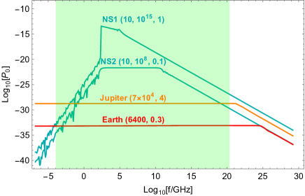
Figure 1: $P_{0}$ as a function of $f=\omega/2\pi$. We show $(r_{0},B_{0})$ for the planets and $(r_{0},B_{0},2\pi/\Omega_{\rm NS})$ for the NSs, where $r_{0}$, $B_{0}$ and $\Omega_{\rm NS}$ (spinning velocity) are in unit of km, Gauss and second^-1, respectively. The green region denotes the EM observation frequency band in astronomy, ranging from radio waves to PeV photons.

For the planets, the plasma density is described by Barometric formula, which yields an exponentially suppressed plasma mass as $r$ increases. If $\omega$ is not too small, we can set $\Delta_{\gamma}\approx\Delta_{\rm vac}$. The radial conversion probability is thus well approximated as (see Supplementary Materials (SM) at Sec. A for details)

$$P_{0}=\left\{\begin{array}[]{ll}\frac{1}{4}\Delta^{2}_{\rm M}(r_{0})\,r^{2}_{0}\propto B_{0}^{2}r_{0}^{2}\,,&\omega\lesssim\omega_{\rm tra}\\ \frac{1}{4}\Delta^{2}_{\rm M}(r_{0})\,r^{2}_{0}\left[\frac{\omega}{\omega_{\rm tra}}\right]^{-\frac{4}{5}}\propto B_{0}^{\frac{2}{5}}r_{0}^{\frac{6}{5}}\omega^{-\frac{4}{5}},&\omega\gtrsim\omega_{\rm tra}\\ \end{array}\right.$$ (8)

where $\omega_{\rm tra}$ is determined by $r_{0}\approx l_{\rm osc}(r_{0})$, corresponding to the transition point of orange and red curves in Fig. 1. These relations can be qualitatively explained with Eq. (4). In the homogeneous magnetic field, an optimal probability $P\approx\Delta_{\rm M}^{2}L^{2}$ can be achieved for $\textrm{sinc}(L/l_{\rm osc})\to 1$ or $l_{\rm osc}\gtrsim L$, a case dubbed as “coherent conversion”, for given $L$. When $l_{\rm osc}$ becomes smaller than $L$, $P$ is suppressed by $l_{\rm osc}^{2}/L^{2}$. Extending this criterion to the planets, we have coherent conversion near their surface for $L\sim r_{0}\lesssim l_{\rm osc}(r_{0})$ or $\omega\lesssim\omega_{\rm tra}$, where $P_{0}\propto\Delta^{2}_{\rm M}(r_{0})r_{0}^{2}\propto B_{0}^{2}r_{0}^{2}$. $P_{0}$ for the Jupiter in this region is then $\sim 10^{4}$ times larger than that of the Earth, as its $B_{0}$ and $r_{0}$ are both ten times larger. For $r_{0}>l_{\rm osc}(r_{0})$, the coherent conversion is suppressed near the planet surface. It can only occur for $r_{*}\approx l_{\rm osc}(r_{*})>r_{0}$, with a reduced rate $P_{0}\sim\Delta^{2}_{\rm M}(r_{*})r_{*}^{2}\propto B_{0}^{2/5}r_{0}^{6/5}\omega^{-4/5}$. As shown in Fig. 1, the frequency band for EM astronomical observations falls entirely into the range of surface coherent conversion for both Earth and Jupiter.

In comparison, due to the large strength of their external magnetic field, the NSs tend to have a suppressed $l_{\rm osc}$. The surface coherent conversion thus becomes difficult to achieve. For the two benchmark NSs in Fig. 1, it takes place between $10^{2}-10^{11}\,$GHz for the NS2, and hardly occurs for the NS1 NS (1). In the high-frequency limit, the vacuum effect dominates. $P_{0}$ is given by the 2nd formula in Eq. (8). At the low-frequency end, the plasma effect becomes dominant, yielding a sine-wiggling $P_{0}$. With the Goldreich-Julian model for the NS plasma density Goldreich and Julian (1969), where $|\Delta_{\rm pla}|\propto n_{c}=\frac{2}{e}\mathbf{\Omega}_{\rm NS}\cdot\mathbf{B}[1-(\Omega_{\rm NS}\,r/c)^{2}\sin^{2}\theta]^{-1}\propto{|\bf B|}$, $|\Delta_{\rm pla}|$ decays more slowly than $\Delta_{\rm vac}$ does as $r$ increases. The coherent conversion then takes place at a larger $r_{*}$, compared to the high-frequency case, yielding a more suppressed $P_{0}$ as $\omega$ decreases Liu et al. .

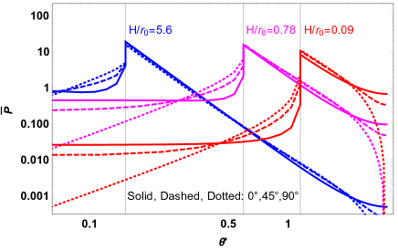
Figure 2: $\bar{P}(\theta^{\prime})$ as a function of $\theta^{\prime}$ for a satellite-based detector. The color and line style denote the normalized altitude $H/r_{0}$ and the latitudes $\lambda_{O^{\prime}}$ respectively for the satellite. The vertical lines denote $\theta_{c}$ for the PC with different $H/r_{0}$ values.

Now let us consider a satellite-based detector positioned at altitude $H$ and latitude $\lambda_{O^{\prime}}$, and define its instant spherical coordinate system with ${\bf\hat{z}}^{\prime}$ pointing to the planet’s center (see SM at Sec. A for details). Then we are able to evaluate the conversion probability $P(\Omega^{\prime})$ of HFGWs traveling to this detector in all directions, where $\Omega^{\prime}=\{\theta^{\prime},\phi^{\prime}\}$. Fig. 2 displays the $\theta^{\prime}$ dependence of $P(\Omega^{\prime})$, with $\bar{P}(\theta^{\prime})=(2\pi P_{0})^{-1}\int_{0}^{2\pi}P(\Omega^{\prime})d\phi^{\prime}$. The signal incoming directions can be split into planet-cone (PC) ($\theta^{\prime}<\theta_{c}=\arcsin[r_{0}/(r_{0}+H)]$) and outer-space (OS) ($\theta^{\prime}>\theta_{c}$) regions, based on whether the line of sight intersects with the planet’s surface. For all sets of $(H/r_{0},\lambda_{O^{\prime}})$, $\bar{P}(\theta^{\prime})$ peaks sharply at the PC edge and drops quickly away from it. For $\lambda_{O^{\prime}}=90^{\circ}$, it drops all the way to zero at $\theta^{\prime}=0$, as $B_{t}$ vanishes in this direction for a detector right above the planet poles. As $H/r_{0}$ increases, with a cost of smaller PC, $\bar{P}(\theta^{\prime})$ tends to have a bigger value inside the PC due to a longer GW-photon conversion path.

III Sensitivity Analysis

The stochastic GWs are typically isotropic and stationary Romano and Cornish (2017). For a detector in the planetary magnetosphere, we have the GW-converted photon flux

$$\Phi_{\gamma}=\int_{\Delta\Omega}d\Omega^{\prime}\int d\omega\frac{h_{c}^{2}}{4\pi\kappa^{2}}P(\Omega^{\prime})\,,$$ (9)

where $\Delta\Omega$ denotes the detector field of view (FOV), and $h_{c}$ is the GW characteristic strain. The signal and background counts for a narrow frequency band $\Delta\omega$, a short observation time $\Delta t$ and an effective detector area $A$ are then given by

$$s \approx \Phi_{\gamma}A\,\Delta t\approx\frac{h_{c}^{2}}{4\pi\kappa^{2}}\langle P\rangle_{\rm det}A\,\Delta t\Delta\omega\Delta\Omega\,,$$

$$b \approx \Phi_{b}A\,\Delta t\approx\phi_{b}A\,\Delta t\Delta\omega\Delta\Omega\,.$$ (10)

Here $\langle P\rangle_{\rm det}=\int_{\Delta\Omega}P(\Omega^{\prime})d\Omega^{\prime}/\Delta\Omega$, essentially determined by the detector position and pointing direction {$\theta’_{\rm det},\phi’_{\rm det}$}, denotes the average GW-photon conversion probability over its FOV. If the detector points to the planet center ($\theta’_{\rm det}=0$), $\langle P\rangle_{\rm det}$ is $\propto\int_{\Delta\Omega}\bar{P}(\theta^{\prime})\sin\theta^{\prime}d\theta^{\prime}/\int_{\Delta\Omega}\sin\theta^{\prime}d\theta^{\prime}$ and increases with $\Delta\Omega$ inside the PC. The 95% upper limit on $h_{c}$ can be derived from $s/\sqrt{b}\approx 1.64$ in the large-background limit:

(11)

In this Letter, we mainly consider the LEO satellite which has a bird view to the dark side of Earth. With the detector FOV restricted to inside the PC, the dominant backgrounds vary from atmospheric thermal emissions in the infrared (IR) band B (29) to cosmic photon albedo (see, e.g., Turler et al. (2010)) throughout the optical - $\gamma$-ray region. We simplify the analysis by assuming a uniform background flux $\phi_{b}$. We will briefly discuss the Jupiter case also. Given the strong angular dependence of $P(\Omega^{\prime})$ (see Fig. 2), an efficient detection requires proper design for satellite orbit and full optimization of detector performance. Below let us consider some specific examples.

	Satellite orbit			Detector properties
	$H$ (km)	$\theta_{\rm inc}$	$T_{\rm dark}$ (s)		IR	UV-Optical	EUV	X-ray	$\gamma$-ray
Conservative	600	$31.4^{\circ}$	$10^{7}$	$\Delta\Omega$ (sr)	$1.6\times 10^{-2}$	$10^{-6}$	$10^{-5}$	$3\times 10^{-5}$	$2.4$
				$A$ ($\rm cm^{2}$)	0.1225	$4.5\times 10^{4}$	1	250	8000
Optimistic	800	$98^{\circ}$	$10^{8}$	$\Delta\Omega$ $(\rm sr)$	3.4	3.4	3.4	3.4	3.4
				$A$ ($\rm cm^{2}$)	0.1	$10^{2}$	$10^{2}$	$10^{2}$	$10^{4}$

Table 1: Benchmark scenarios for sensitivity study. For the conservative case, we take the Suzaku-like low inclination orbit Suz with one year operation. The detector FOV and effective area are assumed to be the same as those of the existing missions including Nimbus Hanel and Chaney (1965) (IR), Hubble Hub (a, b) (ultraviolet (UV)-Optical), Voyager Broadfoot et al. (1977) (extreme UV (EUV)), Suzaku Koyama et al. (2007) (X-ray) and Fermi-LAT Fer ($\gamma-$ray). For the optimistic case, we take the Safir-2-like high inclination orbit Saf with ten year observation. A FOV covering the whole PC is considered. The effective area is set in a way such that the corresponding etendue for the IR, UV-optical, EUV and X-ray bands Förster et al. (2021) is consistent with that of future missions TES ; Law et al. (2015); YUAN et al. (2018); Fan et al. (2022).

We first consider the detection of HFGWs in the Earth’s magnetosphere. Take the Suzaku mission Koyama et al. (2007) as an example. The Suzaku has a low inclination orbit (see Tab. 1). It revolves at low latitude and has a performance relatively insensitive to season alternation. Eq. (11) thus applies approximately for the entire observation period $T_{\rm dark}$. Also, as the Suzaku FOV is small, $\langle P\rangle_{\rm det}$ does not vary much for $\theta’_{\rm det}\ll\theta_{c}$. For $\theta’_{\rm det}=0$ we have $\langle P\rangle_{\rm det}\approx 5\times 10^{-35}$. As for the background flux in the dark side, it has been measured by the Suzaku to be $\phi_{b}\approx 6.3\,\times 10^{-8}\textrm{cm}^{-2}\textrm{s}^{-1}\textrm{keV}^{-1}\textrm{arcmin}^{-2}$ for $\omega\sim 0.5-10\,$keV Koyama et al. (2007). For one-year operation, we have

$$h_{c,95\%} \sim 2\times 10^{-25}\,.$$ (12)

This limit can be scaled to other missions with similar properties, following Eq. (11).

Notably, the satellite at a high inclination orbit has quite different properties. It scans over the high latitude region also, where the conversion probability varies more inside the PC and becomes bigger for a region extending from the PC edge to its inside, compared to the low-latitude case (see Fig. 2). The sensitivity thus could be optimized by taking a detector with either a large FOV covering the whole PC or a small FOV but pointing to the region near the PC edge. Moreover, the observation of such a satellite in the dark side of Earth is sensitive to the season alternation. So we need to generalize Eq. (11) by binning the detector FOV and observation time in this case. The limit shall be obtained from the combined statistics (see SM at Sec. B for details).

Next, we consider the HFGWs conversion in the Jovian magnetosphere. Take Juno, the latest mission orbiting the giant, as an example. The Juno is settled at a highly elliptical polar orbit with a Perijove $\sim 5000\,$km Bloxham et al. (2013) and a high inclination angle ($\sim 90^{\circ}$). For each orbit, the Juno spends a few hours around the Perijove in observing the Jupiter’s cloud. So $\Delta t$ is $\sim 10^{5}\,$s for the $\sim 35$ rounds of its prime mission. As a conservative estimate, we consider the Juno observation of aurora emissions by the Jovian Infrared Auroral Mapper (JIRAM) Adriani et al. (2017a) and UV emissions by the Ultraviolet Spectrograph (UVS) Gladstone et al. (2017), which set respectively $\phi_{b}\sim 4.2\times 10^{4}\,\textrm{cm}^{-2}\textrm{s}^{-1}\textrm{eV}^{-1}\textrm{arcmin}^{-2}$ for $\omega\sim 0.35\,$eV Adriani et al. (2017b) and $\sim 34\,\textrm{cm}^{-2}\textrm{s}^{-1}\textrm{eV}^{-1}\textrm{arcmin}^{-2}$ for $\omega\sim 8\,$eV Giles et al. (2023). We take $\theta^{\prime}_{\rm det}\sim 0.8\theta_{c}$ for $\langle P\rangle_{\rm det}$ and assume $\langle P\rangle_{\rm det}$ to vary little with time. Then, with $\Delta\Omega\sim 10^{-3}\,$sr and $3\times 10^{-4}$ sr, $A\sim 2\,\text{cm}^{2}$ and $6\,\text{cm}^{2}$ and $\Delta\omega\sim 1.4\times 10^{13}\,$Hz and $0.9\times 10^{15}\,$Hz, we have

$$h_{c,95\%}\sim 4\times 10^{-22}\quad{\rm and}\quad 2\times 10^{-23}\,,$$ (13)

for the JIRAM and the UVS, respectively.

As a reference, let us consider the conversion of HFGWs in the NS magnetosphere. The NSs are remote. So we have $\langle P\rangle_{\rm det}\sim P_{0}$ and $\Delta\Omega\sim\pi r_{0}^{2}/d^{2}$, where $d$ is their distance to the Earth. Take the Magnificent Seven (M7) X-ray dim isolated NSs as an example, which have $d\sim\mathcal{O}(100)\,$pc and $B_{0}\sim 10^{13}\,$Gauss, and hence $P_{0}\sim 10^{-18}$ and $\Delta\Omega\sim 10^{-30}\,\textrm{sr}$. The PN and MOS of the XMM-Newton telescope have measured the flux of, e.g., J0420 ($d\approx 345\,$pc), to be $\phi_{b}\sim 10^{17}-10^{19}\,\textrm{cm}^{-2}\textrm{s}^{-1}\textrm{keV}^{-1}\textrm{arcmin}^{-2}$ for $\omega\sim 0.5-1\,$keV, where $A\sim 1500\rm\,cm^{2}$ and $\Delta t\sim 10^{5}\,$s. Such an intensity consists well with the background model of thermal surface emissions Dessert et al. (2020). By applying Eq. (11), we find

$$h_{c,95\%} \sim \mathcal{O}(1)\times 10^{-20}\,.$$ (14)

Due to the extreme smallness of $\Delta\Omega$, this limit is about five orders of magnitude worse than that in Eq. (12). This highlights in part the merit of nearby planets in performing the task of detecting HFGWs.

It is also informative to compare these limits with the ones recast from the existing laboratory experiments for axion detection Ejlli et al. (2019). In these experiments, the magnetic field is typically confined inside a long straight pipe, with a small cross-sectional area. The GW-photon conversion is suppressed outside the small opening angle of long pipe. The signal flux in Eq. (9) is thus strongly limited by the detector geometry (see SM at Sec. C for details). Taking the CERN Axion Solar Telescope (CAST) experiment Anastassopoulos et al. (2017) as an example, we have the recast limit

$$h_{c,95\%}\sim 8\times 10^{-26}\,.$$ (15)

IV Projected sensitivities

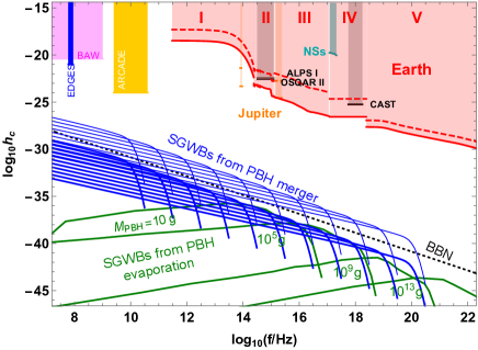
Figure 3: Projected $95\%$ C.L. upper limits on the characteristic strain $h_{c}$ of stochastic HFGWs, set by the LEO satellites (red). We estimate these limits with the Suzaku X-ray measurements Koyama et al. (2007) for band IV, and the IR B (29), UV-optical Hauser and Dwek (2001); Cooray (2016); Scarino et al. (2016); Tilstra et al. (2004), EUV Hill et al. (2018); EUV and $\gamma$-ray Cumani et al. (2019) backgrounds for bands I, II, III and V, respectively. The solid and dashed bottom lines for these bands correspond to the conservative and optimistic estimates defined in Tab. 1. Moreover, we present the conservative and optimistic limits as orange bands, based on the Juno observation of aurora emissions Adriani et al. (2017b) and UV spectra at Jupiter Giles et al. (2023). We also present the limits set by the X-ray observations of M7 NSs Dessert et al. (2020) as cyan band. For completeness, we recast the limits of ALPS, OSQAR and CAST foo (a), i.e., three existing laboratory experiments, as gray bands. We denote the highly-uncertain radio limits of EDGES and ARCADE Aggarwal et al. (2021) as blue and yellow bands foo (b). The black dotted line reflects the BBN constraint on the effective relativistic degrees of freedom in the early Universe Cyburt et al. (2016). As a reference, we present the HFGWs from the Hawking evaporation of highly spinning primordial black holes (PBHs) in the early Universe Anantua et al. (2009); Dolgov and Ejlli (2011); Dong et al. (2016) as green solid lines, and from the binary mergers of PBHs in the Universe after the BBN Franciolini et al. (2022) as thin-solid and solid blue lines for two benchmark scenarios.

To demonstrate the potential of detecting stochastic HFGWs in the planetary laboratory with the LEO satellites, we define two benchmark scenarios, dubbed “conservative” and “optimistic”, in Tab. 1. The choice of orbit in these two scenarios echoes the discussions above on its impacts on the detection efficiency. Fig. 3 shows the projected $95\%$ C.L. limits on the characteristic strain of HFGWs for a wide range of frequencies, including a large portion unexplored before.

In the $\gamma$-ray band, the limits are strengthened with a rate faster than $\sim f^{-1/2}$, due to the reduction of albedo backgrounds Cumani et al. (2019). For the $X$-ray region, the background flux is taken from the Suzaku measurement. Its conservative limits thus represent the first limits from this mission. For the UV-optical band, we consider the cosmic background Hauser and Dwek (2001); Cooray (2016) with a frequency-dependent reflectance of atmosphere Scarino et al. (2016); Tilstra et al. (2004). The limits get nearly one order of magnitude stronger at the right edge of the UV-optical band, due to the ozone absorption of cosmic photons. Such a trend extends to the EUV band, where photodissociation and photoionization become important Fu (2006) and a reflectance of $\sim 10^{-3}$ EUV is thus approximately taken for cosmic photons. As for the IR band, the backgrounds are modelled with a blackbody spectrum at 294K B (29). These thermal radiations peak at $f\sim 10^{13}\,$Hz, and are quickly suppressed for $f>10^{14}\,$Hz. We also present the limits from the observations of Jupiter and NSs in some specific frequency bands. For the optimistic estimate of Jupiter limits, we take $\Delta\Omega=4\,$sr, $A=100\,\text{cm}^{2}$ and $\Delta t=10^{7}\,$s.

V Summary and Outlook

In this Letter, we have proposed to detect the stochastic HFGWs in the planetary magnetosphere. Due to the relatively long path for effective GW-photon conversion, the wide angular distribution of signal flux and a full coverage of the EM observation frequency band in astronomy, this strategy creates a new operation space. With the proof of concept presented, we can immediately see several important directions for next-step explorations.

Firstly, extend the detection of HFGWs from the PC to the OS. As indicated by Fig. 2, the GW-photon conversion probability right outside the PC can be much higher than that inside. Moreover, a detector oriented toward the OS may receive considerably less atmospheric thermal radiation. The relevant sensitivities in Fig. 3 thus could be significantly improved. Secondly, extend the satellite-based detection to terrestrial observations, which may allow the sensitivities to cover the radio bands. Thirdly, extend the dedicated study to the Jupiter and even the Sun, given their stronger magnetic field, larger space for an effective GW-photon conversion, and the active and upcoming missions. We leave these explorations to a paper in preparation Liu et al. .

Acknowledgments

We would greatly thank Lian Tao for discussion on the properties of satellites and X-ray telescopes and A. Ejlli for communications on the recast limits of laboratory experiments. T. Liu and C. Zhang are supported by the Collaborative Research Fund under Grant No. C6017-20G which is issued by Research Grants Council of Hong Kong S. A. R. J. Ren is supported by the Institute of High Energy Physics, Chinese Academy of Sciences, under Contract No. Y9291220K2.

Appendix A Supplemental Material

The Supplementary Materials contain additional calculations and explanations in support of the results presented in this Letter. Concretely, we discuss the GW-photon conversion in planetary magnetosphere in Sec. A, analyze the impacts of the orbit design for the LEO satellites on the HFGWs detection in Sec. B, and calculate the recast limits from the laboratory experiments in Sec. C.

A.1 A. GW-Photon Conversion in Planetary Magnetosphere

As gravity couples with EM dynamics via $\sim g^{\mu\nu}T_{\mu\nu}^{\rm EM}$, the GWs can be converted to photons while propagating in an external magnetic field $\mathbf{B}$. The leading-order equations of motion are given by Raffelt and Stodolsky (1988); Ejlli and Thandlam (2019)

$$\left(\omega-i\partial_{n}+\left(\begin{array}[]{cccc}\Delta_{\perp}&\Delta_{M}&\Delta_{R}&0\\ \Delta_{M}&0&0&0\\ \Delta_{R}&0&\Delta_{||}&\Delta_{M}\\ 0&0&\Delta_{M}&0\end{array}\right)\right)\left(\begin{array}[]{c}A_{||}\\ G_{\times}\\ A_{\perp}\\ G_{+}\end{array}\right)=0\,.$$ (24)

(25)

Here $G_{\times}$ and $G_{+}$ denote the cross and plus polarization modes of GWs; $A_{||}$ and $A_{\perp}$ denote the polarization modes of photons parallel with and perpendicular to $\mathbf{B_{T}}$, the $\mathbf{B}$ component transverse to the GW propagation direction. In the $4\times 4$ propagation matrix,

$$\Delta_{||} = \Delta_{\textrm{pla}}+\Delta_{\textrm{vac},||}+\Delta_{\textrm{CM}}\,$$

$$\Delta_{\perp} = \Delta_{\textrm{pla}}+\Delta_{\textrm{vac},\perp}\,$$ (26)

denote an effective mass of $A_{||}$ and $A_{\perp}$, respectively. Here

$$\Delta_{\rm pla} = -\frac{m_{\rm pla}^{2}}{2\omega}\,,$$

$$\Delta_{\textrm{vac},||(\perp)} = 7(4)\frac{\alpha\omega}{90\pi}\left(\frac{B_{t}}{B_{c}}\right)^{2}$$ (27)

encode the plasma and QED vacuum effects, and $\Delta_{\rm CM}\propto B_{t}^{2}$ Ejlli and Thandlam (2019) can induce Cotton-Mouton birefringence. $m_{\rm pla}^{2}=4\pi\alpha n_{c}/m_{c}$ is plasma mass square, with $n_{c}$ and $m_{c}$ being the number density and invariant mass of charged plasma particles. Moreover, the $\Delta_{R}$ term, which is proportional to $\mathbf{B}-\mathbf{B_{T}}$, couples $A_{||}$ and $A_{\perp}$ and can yield Faraday rotation. The GW-photon mixing, which is a core of this study, is governed by $\Delta_{\rm M}=\frac{1}{2}\kappa B_{t}$, where $B_{t}=|\mathbf{B_{T}}|$.

For the GW-photon conversion in planetary magnetosphere where $\omega$ of interest (see Fig. 3) is mostly larger than the cyclotron angular frequency $\omega_{c}\approx 10^{7}(|\mathbf{B}|/\rm Gauss)$ Hz, $\Delta_{\rm CM}$ and $\Delta_{R}$ are negligibly small compared to $\Delta_{\rm pla}$ Ejlli and Thandlam (2019). Thus, the equations in Eq. (25) can be separated to two decoupled ones, for the polarization modes $\{A_{||},G_{\times}\}$ and $\{A_{\perp},G_{+}\}$, respectively. For simplicity, one can further neglect the small difference between $\Delta_{\textrm{vac},||}$ and $\Delta_{\textrm{vac},\perp}$, and assume $\Delta_{\textrm{vac},||}=\Delta_{\textrm{vac},\perp}=\Delta_{\textrm{vac}}$. The two propagating equations then share the same form and become

$$\left(\omega-i\partial_{n}+\left(\begin{array}[]{cc}\Delta_{\gamma}&\Delta_{\rm M}\\ \Delta_{\rm M}&0\end{array}\right)\right)\left(\begin{array}[]{cc}A_{||(\perp)}\\ G_{\times(+)}\\ \end{array}\right)=0\,,$$ (32)

where $\Delta_{\gamma}\approx\Delta_{\rm vac}+\Delta_{\rm pla}$. This gives exactly the mixing matrix in Eq. (3).

Due to the smallness of gravitational coupling, we have $\Delta_{\rm M}\ll\Delta_{\gamma}$ and hence $l_{\rm osc}=2/(4\Delta_{\rm M}^{2}+\Delta_{\gamma}^{2})^{1/2}\approx 2/\Delta_{\gamma}$ in general. This implies a weak mixing between the GWs and photons. Nonetheless, $\Delta_{\rm vac}$ and $\Delta_{\rm pla}$ have opposite signs, and a maximum mixing can be realized if the two cancel well such that $\Delta_{\gamma}\ll\Delta_{\rm M}$. In the planetary magnetosphere, such a cancellation might be possible only for a tiny range of the GW traveling path. Its contribution to the total conversion probability is typically negligible. Instead, the “coherent conversion”, where the conversion probability is maximized for given magnetic field and GW path, tends to be realized for a longer part of the path and hence contribute more to the GW-photon conversion.

To have a taste, in the main text we first analyze the GW-photon conversion for a radial path of the planets from zero altitude and latitude to spatial infinity. Due to the difference in spinning velocity, the plasma density of planets is described by Barometric formula

$$n_{c}^{\rm Bar}=n_{c,0}\exp\left(-\frac{r-r_{0}}{H_{\rm cor}}\right)\,,$$ (33)

where $H_{\rm cor}\ll r_{0}$ denotes the scale height, with $H_{\rm cor}\approx 8.4\,(27)\textrm{ km}$ for Earth (Jupiter), while the plasma density of NSs is described by Goldreich-Julian model Goldreich and Julian (1969). As $n_{c}^{\rm Bar}$ is exponentially suppressed at $r-r_{0}\gg H_{\rm cor}$, the plasma mass contribution is mostly negligible along the path for the GW frequency of interest. Thus, we focus on the vacuum effect and assume $\Delta_{\gamma}=\Delta_{\rm vac}$. $P_{0}$ then can be solved exactly as Dessert et al. (2019); Fortin and Sinha (2019); Fortin et al. (2021)

$$P_{0}\approx\frac{(\Delta_{M}(r_{0})r_{0})^{2}}{(\Delta_{\rm vac}(r_{0})r_{0})^{\frac{4}{5}}}\left|\frac{\Gamma(\frac{2}{5})-\Gamma(\frac{2}{5},-\frac{i}{5}\,\Delta_{\rm vac}(r_{0})r_{0})}{5^{\frac{3}{5}}}\right|^{2}\,,$$ (34)

where $\Gamma(z)$ is gamma function and $\Gamma(a,z)$ is incomplete gamma function. $\Delta_{\rm M}(r_{0})$ and $\Delta_{\rm vac}(r_{0})$ are defined at the planet surface where $r=r_{0}$.

In the low frequency limit, where $\Delta_{\rm vac}(r_{0})\,r_{0}\lesssim 1$ and hence $r_{0}\lesssim l_{\rm osc}(r_{0})$, the coherent conversion can be achieved near the planet surface. Eq. 34 then gives the first formula in Eq. (8):

$$P_{0} \approx \frac{1}{4}\Delta^{2}_{M}(r_{0})r^{2}_{0}$$ (35)

$$= 2.1\times 10^{-32}\left(\frac{B_{0}}{1\,\textrm{Gauss}}\right)^{2}\left(\frac{r_{0}}{10^{4}\,\textrm{km}}\right)^{2}\,.$$

This implies that $P_{0}$ receives more contributions from the low altitude region.

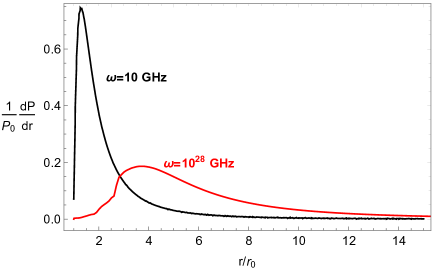
Figure 4: $\frac{1}{P_{0}}\frac{dP(r)}{dr}$ as a function of $r/r_{0}$ for the Earth ($\omega_{\textrm{tra}}\approx 10^{25}\textrm{GHz}$). The black and red curves denote the low-frequency ($\omega=10$ GHz) and high-frequency ($\omega=10^{28}$ GHz) scenarios, respectively.

In the high frequency limit, where $\Delta_{\rm vac}(r_{0})\,r_{0}\gtrsim 1$ and hence $r_{0}\gtrsim l_{\rm osc}(r_{0})$, the coherent conversion can not be achieved at the Earth surface. Eq. (34) then gives the second formula in Eq. (8):

$$P_{0} \approx 0.7\frac{(\Delta_{M}(r_{0})\,r_{0})^{2}}{(\Delta_{\rm vac}(r_{0})\,r_{0})^{\frac{4}{5}}}=\frac{1}{4}\Delta^{2}_{M}(r_{0})r^{2}_{0}\left(\frac{\omega}{\omega_{\textrm{tra}}}\right)^{-\frac{4}{5}}\,,$$ (36)

where the transition frequency

$$\omega_{\textrm{tra}}\approx 3\times 10^{6}\left(\frac{B_{0}}{10^{10}{\rm Gauss}}\right)^{2}{\rm GHz}$$ (37)

is determined by $\Delta_{\rm vac}(r_{0})\,r_{0}\approx 1$. Eq. (36) matches to Eq. (35) smoothly at $\omega=\omega_{\textrm{tra}}$. In this limit however the coherent conversion can be realized above the planet surface, where $r=r_{*}>r_{0}$. $r_{*}$ can be estimated by solving $\Delta_{\rm vac}(r_{*})r_{*}=1$. With $\Delta_{M}(r)=\Delta_{M}(r_{0})(r_{0}/r)^{3}$ and $\Delta_{\rm vac}(r)=\Delta_{\rm vac}(r_{0})(r_{0}/r)^{6}$, we obtain $r_{*}=r_{0}(\Delta_{\rm vac}(r_{0})r_{0})^{1/5}$. This implies that $P_{0}$ here receives more contributions at $r\gtrsim r_{*}$. These features are shown in Fig. 4 for the Earth. Indeed, in the high-frequency case, the curve peaks near $r_{*}/r_{0}\approx 10^{-5}(\omega/\text{GHz})^{1/5}$.

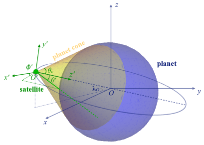
Figure 5: Instant coordinate system for a satellite-based detector. $\{x,y,z\}$ and $\{x^{\prime},y^{\prime},z^{\prime}\}$ are the coordinate systems centered at the planet center $O$ and the satellite location $O^{\prime}$, respectively, with $z$ axis and $z^{\prime}$ axis respectively oriented towards the planet north pole and center. $\lambda_{O^{\prime}}$ denotes the latitude of the satellite. $\theta_{c}$ is the open angle of the PC that is tangential to the planet’s surface. $\theta^{\prime}$ and $\phi^{\prime}$ are the polar and azimuthal angles of the line of sight (solid green line) defined in the $\{x^{\prime},y^{\prime},z^{\prime}\}$ frame, respectively.

For sensitivity demonstration, we consider a satellite-based detector. The instant coordinate system for this detector is displayed in Fig. 5. As the GW-photon conversion probability $P(\Omega^{\prime})$ exhibits a stronger dependence on $\theta^{\prime}$ than on $\phi^{\prime}$, it is convenient to show its $\theta^{\prime}$ dependence in Fig. 2, by integrating out $\phi^{\prime}$.

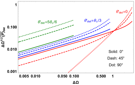
Figure 6: $\Delta\Omega^{1/2}\overline{\langle P\rangle}_{\rm det}/P_{0}$ as a function of $\Delta\Omega$ for a satellite-based detector at $H/r_{0}=0.16$, where $\overline{\langle P\rangle}_{\rm det}=\int_{0}^{2\pi}{\langle P\rangle}_{\rm det}d\phi^{\prime}_{\rm det}/(2\pi P_{0})$ is an average $\langle P\rangle_{\rm det}$ over $\phi^{\prime}_{\rm det}$. The line style and color denote the satellite latitude $\lambda_{O^{\prime}}$ and the detector pointing direction $\theta^{\prime}_{\rm det}$, respectively.

As shown in Eq. (11), the limits on $h_{c}$ are sensitive to the satellite position, the detector pointing direction {$\theta’_{\rm det},\phi’_{\rm det}$} and its FOV $\Delta\Omega$. Considering $h_{c,95\%}\propto\Delta\Omega^{1/2}\langle P\rangle_{\rm det}$, we show in Fig. 6 $\Delta\Omega^{1/2}\overline{\langle P\rangle}_{\rm det}$ as a function of $\Delta\Omega$ for different satellite latitudes and detector pointing directions $\theta^{\prime}_{\rm det}$. For each curve, the quantity increases monotonically with $\Delta\Omega$ in general, and approximately scales as $\Delta\Omega^{1/2}$ for small FOV. As for the $\theta^{\prime}_{\rm dec}$ dependence, the curves change more drastically for the high latitude satellite, in accordance with the angular dependence shown in Fig. 2. $\Delta\Omega^{1/2}\overline{\langle P\rangle}_{\rm det}$ reaches its maximum when the satellite operates at $\lambda_{O^{\prime}}=90^{\circ}$, with the detector FOV covers the whole PC region. As the PC edge contributes more to the signal rate, a sensitivity of the same level could be also obtained for a detector with relatively small FOV but pointing to the PC edge.

A.2 B. Low Earth Orbits for Satellites

For a satellite-based detector, the signal and background photon fluxes are direction and time dependent. To evaluate the orbit quality accurately and hence optimize its design, one can bin the events w.r.t. direction and time while analyzing the sensitivity reach. Eq. (III) is then generalized to

$$s_{ij} = \frac{h_{c}^{2}}{4\pi\kappa^{2}}A\,\Delta t_{j}\Delta\omega P_{\Delta\Omega_{i}}(\Delta t_{j})\,,$$

$$b_{ij} = \phi_{b}(\Delta\Omega_{i},\Delta t_{j})A\,\Delta t_{j}\Delta\Omega_{i}\Delta\omega\,,$$ (38)

for the $i$-th angular and $j$-th time bin. Given the count of observed events $n_{ij}$, the exclusion limit on $h_{c}$ is set by the test statistic Cowan et al. (2011)

$$q(h_{c})=2\sum_{i,j}\left[n_{ij}\ln\frac{n_{ij}}{s_{ij}+b_{ij}}+s_{ij}+b_{ij}-n_{ij}\right]\,,$$ (39)

which is Poisson-statistics-based and defined against the background + signal ($h_{c}$) hypothesis. The projected $95\%$ C.L. upper limit on $h_{c}$ is then obtained by requesting $q(h_{c,95\%})|_{n=b}=2.7$, where $n_{ij}$ is assumed to be the same as the predicted background count. In the Gaussian statistics, Eq. (39) is reduced to $q(h_{c})=\sum_{i,j}s_{ij}^{2}/(b_{ij}+s_{ij})$. It can be further simplified to $q(h_{c})=\sum_{i,j}s_{ij}^{2}/b_{ij}$ in the limit of large background, where $b_{ij}\gg s_{ij}$. This yields the criteria of $s/\sqrt{b}=1.64$ for the one-bin analysis, which has been applied for the derivation of Eq. (11).

	$H$ (km)	$\theta_{\rm inc}$	$\psi$	$T$ (mins)
Suzaku-like Suz	600	$31.4^{\circ}$	$79.7^{\circ}$	90
SAFIR 2-like Saf	800	$98^{\circ}$	$257^{\circ}$	101

Table 2: Two LEO benchmark scenarios. $H$ is orbit altitude, $\theta_{\rm inc}$ is inclination angle, $\psi$ is right ascension of the ascending node, and $T$ is orbit period.

To have a taste on the impacts of orbit design, let us consider two benchmark scenarios defined in Tab. 2. In Scenario I, the orbit is Suzaku-like, characterized by a low inclination angle. As the detector is restricted to revolve in the low latitude region ($|\lambda_{O^{\prime}}|\lesssim 30^{\circ}$), the total time for its staying in the orbit of dark side, dubbed “dark orbit”, varies little with the season alternation. This yields an overall fraction $f_{\rm dark}\approx 0.35$ or equivalently effective observation time $T_{\rm dark}\approx 1.1\times 10^{7}\,$s for one-year revolution. In scenario II, the orbit is SAFIR 2-like, characterized by a high inclination angle. As the detector can reach the high-latitude region, the signal rate fluctuates more during each orbit period. The total time for its revolving in the dark orbit varies strongly with the season alternation. For one-year revolution, we have an overall fraction $f_{\rm dark}\approx 0.2$ and effective observation time $T_{\rm dark}\approx 6.3\times 10^{6}\,$s.

Figure 7: $q(h_{c})|_{n=b}$ as a function of $h_{c}$ in Suzaku-like (blue) and SAFIR 2-like (red) scenarios for 10-year revolution. The dashed line denotes the $q(h_{c})|_{n=b}$ value at 95% C.L.

To bin the event count in each benchmark scenario, we divide the dark orbit by a time interval $\Delta t=120$ s. Also, we consider the full PC region as the detector FOV and separate it into four concentric circular belts. We then evaluate $q(h_{c})|_{n=b}$ by taking a summation of $s_{ij}$ and $b_{ij}$ over the time-angular bins for 10-year revolution. Finally we display the test statistic $q(h_{c})|_{n=b}$ in Fig. 7 as a function of $h_{c}$ for these two scenarios (with $A=250\,\rm cm^{2}$). The SAFIR 2-like orbit has a better sensitivity performance, although it spends less time in the dark orbit. This could be attributed to a larger GW-photon conversion probability off the PC center while the detector revolves in the high-latitude region (see Fig. 2). Also, as one merit of high-inclination orbit, the dark-orbit time is mainly contributed by the polar-night season, enabling a more efficient usage of the telescope resources.

A.3 C. Recast Limits from Laboratory Experiments

The limits obtained in the laboratory experiments for axion detection can be recast to constrain the HFGWs (for a review, see Aggarwal et al. (2021)). Since the magnetic field in these experiments is often confined inside a straight-long cylinder pipe, the conversion probability of stochastic HFGWs into photons exhibits a strong angular dependence. This will necessarily influence the estimate of the GW-converted photon flux in Eq. (9).

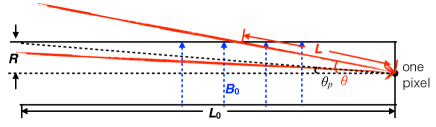
Figure 8: Schematic for the GW-photon conversion in a straight-long cylinder pipe which has a length $L_{0}$, a cross-sectional area $A=\pi R^{2}$ and an internal magnetic field ${\bf B}_{0}$ (with $B_{0}=|{\bf B}_{0}|$). The black dot denotes the central pixel of the detector at the right end of the pipe. The red lines denote the incoming GWs. These GWs travel in the pipe by a distance $L$, in a direction with $0\leq\theta<\pi/2$. $\theta_{p}\approx R/L_{0}\ll 1$ denotes the opening angle of pipe.

Explicitly, let us consider the coherent conversion in an experimental facility shown in Fig. 8. For the central pixel of its detector, the angular integral in Eq. (9) reduces to an integration over $\theta$, which can be put into two parts. The first one accounts for the signals received in the opening angle, where $0\leq\theta\leq\theta_{p}$. As $P(\theta)\propto L^{2}B_{t}^{2}=(L_{0}/\cos\theta)^{2}(B_{0}\cos\theta)^{2}=L_{0}^{2}B_{0}^{2}$, the conversion probability is insensitive to $\theta$. However, for the signals outside the opening angle, where $\theta_{p}<\theta<\pi/2$, $P(\theta)$ shows a strong dependence on $\theta$, as $P(\theta)\propto L^{2}B_{t}^{2}=(R/\sin\theta)^{2}(B_{0}\cos\theta)^{2}=R^{2}B_{0}^{2}/\tan^{2}\theta$. The integrated flux at this pixel is then

$$\Phi_{\gamma} \approx \frac{\kappa^{2}B_{0}^{2}}{4}\frac{\Delta\omega\,h_{c}^{2}}{4\pi\kappa^{2}}\int_{0}^{2\pi}d\phi\Big{(}L_{0}^{2}\int_{0}^{\theta_{p}}\sin\theta d\theta$$ (40)

$$+ R^{2}\int_{\theta_{p}}^{\pi/2}\frac{\sin\theta d\theta}{\tan^{2}\theta}\Big{)}$$

$$\approx \frac{1}{8}\Delta\omega h_{c}^{2}B_{0}^{2}L_{0}^{2}\theta_{p}^{2}\ln\frac{1}{\theta_{p}}\,.$$

A limit of $\theta_{p}\ll 1$ is taken in the last line. Note, the $\phi$ dependence of $B_{t}$ has not been considered in this derivation. It can be shown that this effect is tiny for Eq. (40) in the small $\theta_{p}$ limit. Similar derivation can be applied to other pixels of the detector. For the experiments listed in Tab. 3, where $\theta_{p}$ is consistently small, we have verified numerically that the results for all pixels can be approximated by the leading-order term in Eq. (40), with a deviation up to $\mathcal{O}(10\%)$. Thus, the GW-converted photon flux in the detector is estimated as

$$\Phi_{\gamma}\sim\Phi^{0}_{\gamma}\frac{\Delta\Omega_{p}}{\pi}\frac{1}{4}\ln\frac{\pi}{\Delta\Omega_{p}}\,,$$ (41)

where for a narrow frequency band

$$\Phi^{0}_{\gamma}\approx\frac{1}{4}{B_{0}^{2}\,L_{0}^{2}\,h_{c}^{2}\,\Delta\omega}\,.$$ (42)

Note that $\Phi_{\gamma}$ is subject to a suppression of pipe geometry denoted by

$$\Delta\Omega_{p}\approx\frac{A}{L_{0}^{2}}\approx\pi\theta_{p}^{2}\,.$$ (43)

	$N_{\rm exp}$ (mHz)	$A$ (${\rm m}^{2}$)	$L_{0}$ (m)	$B_{0}$ (T)	$\Delta f$ (Hz)
CAST	0.15	0.0029	$9.3$	$9$	$10^{18}$
ALPS I	0.61	0.005	$9$	$5$	$9\times 10^{14}$
OSQAR II	1.1	0.005	$14$	$9$	$10^{15}$

Table 3: Baseline parameters for some laboratory experiments Ejlli et al. (2019) relevant to this study.

The upper limits on $h_{c}$ can be obtained by comparing the signal rate $\Delta s/\Delta t$ with the observed event rate $N_{\rm exp}$ (see Tab. 3), which gives

$$h_{c,95\%}\approx\frac{4}{B_{0}A}\sqrt{\frac{\pi N_{\rm exp}}{\Delta\omega\ln(\pi L_{0}^{2}/A)}}\,.$$ (44)

Then we have the limits shown in Fig. 3: $h_{c,95\%}\sim 8\times 10^{-26}$ for the CAST (see Eq. (15) also), and $h_{c,95\%}\sim 5\times 10^{-23}\,$ and $4\times 10^{-23}\,$ for the ALPS I and the OSQAR II, respectively.

References

- Abbott et al. (2016) B. P. Abbott et al. (LIGO Scientific, Virgo), Phys. Rev. Lett. 116, 061102 (2016), eprint 1602.03837.
- Aggarwal et al. (2021) N. Aggarwal et al., Living Rev. Rel. 24, 4 (2021), eprint 2011.12414.
- Lommen (2015) A. N. Lommen, Reports on Progress in Physics 78, 124901 (2015).
- Tiburzi (2018) C. Tiburzi, Publications of the Astronomical Society of Australia 35 (2018), URL https://doi.org/10.1017%2Fpasa.2018.7.
- Renzini et al. (2022) A. I. Renzini, B. Goncharov, A. C. Jenkins, and P. M. Meyers, Galaxies 10, 34 (2022), eprint 2202.00178.
- Gertsenshtein (1962) M. Gertsenshtein, Sov. Phys. JETP 14, 84 (1962).
- Lupanov (1967) G. A. Lupanov, Sov. Phys. JETP 25, 76 (1967).
- Boccaletti (1970) D. Boccaletti, Nuovo Cimento 70 B, 129 (1970).
- Zeldovich (1973) Y. B. Zeldovich, Sov. Phys. JETP 65, 1311 (1973).
- De Logi and Mickelson (1977) W. K. De Logi and A. R. Mickelson, Phys. Rev. D 16, 2915 (1977).
- Raffelt and Stodolsky (1988) G. Raffelt and L. Stodolsky, Phys. Rev. D 37, 1237 (1988).
- Chen (1995) P. Chen, Phys. Rev. Lett. 74, 634 (1995), [Erratum: Phys.Rev.Lett. 74, 3091 (1995)].
- Cillis and Harari (1996) A. N. Cillis and D. D. Harari, Phys. Rev. D 54, 4757 (1996), eprint astro-ph/9609200.
- Pshirkov and Baskaran (2009) M. S. Pshirkov and D. Baskaran, Phys. Rev. D 80, 042002 (2009), eprint 0903.4160.
- Domcke and Garcia-Cely (2021) V. Domcke and C. Garcia-Cely, Phys. Rev. Lett. 126, 021104 (2021), eprint 2006.01161.
- Ramazanov et al. (2023) S. Ramazanov, R. Samanta, G. Trenkler, and F. R. Urban (2023), eprint 2304.11222.
- Berlin et al. (2021) A. Berlin, D. Blas, R. Tito D’Agnolo, S. A. R. Ellis, R. Harnik, Y. Kahn, and J. Schütte-Engel (2021), eprint 2112.11465.
- Aguiar (2011) O. D. Aguiar, Res. Astron. Astrophys. 11, 1 (2011), eprint 1009.1138.
- Harry et al. (1996) G. M. Harry, T. R. Stevenson, and H. J. Paik, Phys. Rev. D 54, 2409 (1996), eprint gr-qc/9602018.
- Herman et al. (2020) N. Herman, A. Füzfa, S. Clesse, and L. Lehoucq (2020), eprint 2012.12189.
- Herman et al. (2022) N. Herman, L. Lehoucq, and A. Fúzfa (2022), eprint 2203.15668.
- Domcke et al. (2022) V. Domcke, C. Garcia-Cely, and N. L. Rodd, Phys. Rev. Lett. 129, 041101 (2022), eprint 2202.00695.
- Ringwald et al. (2021) A. Ringwald, J. Schütte-Engel, and C. Tamarit, JCAP 03, 054 (2021), eprint 2011.04731.
- Ejlli et al. (2019) A. Ejlli, D. Ejlli, A. M. Cruise, G. Pisano, and H. Grote, Eur. Phys. J. C 79, 1032 (2019), eprint 1908.00232.
- Li et al. (2000) F.-Y. Li, M.-X. Tang, J. Luo, and Y.-C. Li, Phys. Rev. D 62, 044018 (2000).
- Li et al. (2003) F.-Y. Li, M.-X. Tang, and D.-P. Shi, Phys. Rev. D 67, 104008 (2003), eprint gr-qc/0306092.
- Li and Yang (2004) F.-Y. Li and N. Yang, Chin. Phys. Lett. 21, 2113 (2004), eprint gr-qc/0410060.
- Li et al. (2006) F. Li, R. M. L. Baker, Jr., and Z. Chen (2006), eprint gr-qc/0604109.
- Li et al. (2008) F. Li, R. M. L. Baker, Jr., Z. Fang, G. V. Stephenson, and Z. Chen, Eur. Phys. J. C 56, 407 (2008), eprint 0806.1989.
- Tong et al. (2008) M.-l. Tong, Y. Zhang, and F.-Y. Li, Phys. Rev. D 78, 024041 (2008), eprint 0807.0885.
- Stephenson (2009) G. V. Stephenson, AIP Conf. Proc. 1103, 542 (2009).
- Li et al. (2009) F. Li, N. Yang, Z. Fang, R. M. L. Baker, Jr., G. V. Stephenson, and H. Wen, Phys. Rev. D 80, 064013 (2009), eprint 0909.4118.
- Li et al. (2011) J. Li, K. Lin, F. Li, and Y. Zhong, Gen. Rel. Grav. 43, 2209 (2011).
- Li et al. (2013) F.-Y. Li, H. Wen, and Z.-Y. Fang, Chin. Phys. B 22, 120402 (2013).
- Li et al. (2016a) J. Li, L. Zhang, K. Lin, and H. Wen, Int. J. Theor. Phys. 55, 3506 (2016a), eprint 1411.1811.
- Li et al. (2016b) J. Li, L. Zhang, and H. Wen, Int. J. Theor. Phys. 55, 1871 (2016b).
- Li et al. (2023) F.-Y. Li, H. Yu, J. Li, L.-F. Wei, and Q.-Q. Jiang (2023), eprint 2303.03974.
- Berlin et al. (2023) A. Berlin, D. Blas, R. Tito D’Agnolo, S. A. R. Ellis, R. Harnik, Y. Kahn, J. Schütte-Engel, and M. Wentzel (2023), eprint 2303.01518.
- Zioutas et al. (1998) K. Zioutas, D. J. Thompson, and E. A. Paschos, Phys. Lett. B 443, 201 (1998), eprint astro-ph/9808113.
- Davoudiasl and Huber (2006) H. Davoudiasl and P. Huber, Phys. Rev. Lett. 97, 141302 (2006), eprint hep-ph/0509293.
- Davoudiasl and Huber (2008) H. Davoudiasl and P. Huber, JCAP 08, 026 (2008), eprint 0804.3543.
- Feng et al. (2016) J. L. Feng, J. Smolinsky, and P. Tanedo, Phys. Rev. D 93, 015014 (2016), [Erratum: Phys.Rev.D 96, 099901 (2017)], eprint 1509.07525.
- Leane and Linden (2021) R. K. Leane and T. Linden (2021), eprint 2104.02068.
- Li and Fan (2022) L. Li and J. Fan, JHEP 10, 186 (2022), eprint 2207.13709.
- French and Sher (2022) G. M. French and M. Sher (2022), eprint 2210.04761.
- Irastorza and Redondo (2018) I. G. Irastorza and J. Redondo, Prog. Part. Nucl. Phys. 102, 89 (2018), eprint 1801.08127.
- NS (1) For NS1 with GHz, the dominant contribution to arises from the integration over a specific tiny range of , where a maximal mixing is achieved with a strong cancellation between and in .
- Goldreich and Julian (1969) P. Goldreich and W. H. Julian, Astrophys. J. 157, 869 (1969).
- (49) T. Liu, J. Ren, and C. Zhang, in preparation.
- Romano and Cornish (2017) J. D. Romano and N. J. Cornish, Living Rev. Rel. 20, 2 (2017), eprint 1608.06889.
- B (29) https://www.giss.nasa.gov/research/briefs/2010_schmidt_05/.
- Turler et al. (2010) M. Turler, M. Chernyakova, T. J. L. Courvoisier, P. Lubinski, A. Neronov, N. Produit, and R. Walter, Astron. Astrophys. 512, A49 (2010), eprint 1001.2110.
- (53) https://in-the-sky.org/spacecraft.php?id=28773.
- Hanel and Chaney (1965) R. Hanel and L. Chaney, NASA Goddard Space Flight Center Document X-650-65-75 (1965).
- Hub (a) https://www.nasa.gov/content/observatory-instruments-advanced-camera-for-surveys.
- Hub (b) https://www.nasa.gov/mission_pages/hubble/spacecraft/index.html.
- Broadfoot et al. (1977) A. Broadfoot, B. Sandel, D. Shemansky, S. Atreya, T. Donahue, H. Moos, J.-L. Bertaux, J.-E. Blamont, J. Ajello, D. Strobel, et al., Space Science Reviews 21, 183 (1977).
- Koyama et al. (2007) K. Koyama, H. Tsunemi, T. Dotani, M. W. Bautz, K. Hayashida, T. G. Tsuru, H. Matsumoto, Y. Ogawara, G. R. Ricker, J. Doty, et al., Publications of the Astronomical Society of Japan 59, S23 (2007).
- (59) https://fermi.gsfc.nasa.gov/ssc/data/analysis/documentation/Cicerone/Cicerone_Introduction/LAT_overview.html.
- (60) https://in-the-sky.org/spacecraft.php?id=25399.
- Förster et al. (2021) F. Förster et al., Astron. J. 161, 242 (2021), eprint 2008.03303.
- (62) https://heasarc.gsfc.nasa.gov/docs/tess/the-tess-space-telescope.html.
- Law et al. (2015) N. M. Law, O. Fors, J. Ratzloff, P. Wulfken, D. Kavanaugh, D. J. Sitar, Z. Pruett, M. N. Birchard, B. N. Barlow, K. Cannon, et al., Publications of the Astronomical Society of the Pacific 127, 234 (2015), URL https://doi.org/10.1086%2F680521.
- YUAN et al. (2018) W. YUAN et al., SCIENTIA SINICA Physica, Mechanica & Astronomica 48, 039502 (2018).
- Fan et al. (2022) Y. Z. Fan, J. Chang, J. H. Guo, Q. Yuan, Y. M. Hu, X. Li, C. Yue, G. S. Huang, S. B. Liu, C. Q. Feng, et al., Acta Astronomica Sinica 63, 27 (2022).
- Bloxham et al. (2013) J. Bloxham, J. E. Connerney, and J. L. Jorgensen, in AGU Fall Meeting Abstracts (2013), vol. 2013, pp. GP54A–03.
- Adriani et al. (2017a) A. Adriani, G. Filacchione, T. Di Iorio, D. Turrini, R. Noschese, A. Cicchetti, D. Grassi, A. Mura, G. Sindoni, M. Zambelli, et al., Space Science Reviews 213, 393 (2017a).
- Gladstone et al. (2017) G. R. Gladstone, S. C. Persyn, J. S. Eterno, B. C. Walther, D. C. Slater, M. W. Davis, M. H. Versteeg, K. B. Persson, M. K. Young, G. J. Dirks, et al., Space Science Reviews 213, 447 (2017).
- Adriani et al. (2017b) A. Adriani, A. Mura, M. Moriconi, B. Dinelli, F. Fabiano, F. Altieri, G. Sindoni, S. Bolton, J. Connerney, S. Atreya, et al., Geophysical Research Letters 44, 4633 (2017b).
- Giles et al. (2023) R. S. Giles, V. Hue, T. K. Greathouse, G. R. Gladstone, J. A. Kammer, M. H. Versteeg, B. Bonfond, D. C. Grodent, J.-C. Gé rard, J. A. Sinclair, et al., Journal of Geophysical Research: Planets 128 (2023), URL https://doi.org/10.1029%2F2022je007610.
- Dessert et al. (2020) C. Dessert, J. W. Foster, and B. R. Safdi, The Astrophysical Journal 904, 42 (2020), URL https://doi.org/10.3847%2F1538-4357%2Fabb4ea.
- Anastassopoulos et al. (2017) V. Anastassopoulos et al. (CAST), Nature Phys. 13, 584 (2017), eprint 1705.02290.
- Hauser and Dwek (2001) M. G. Hauser and E. Dwek, Ann. Rev. Astron. Astrophys. 39, 249 (2001), eprint astro-ph/0105539.
- Cooray (2016) A. Cooray (2016), eprint astro-ph.CO/1602.03512.
- Scarino et al. (2016) B. R. Scarino, D. R. Doelling, P. Minnis, A. Gopalan, T. Chee, R. Bhatt, C. Lukashin, and C. Haney, IEEE Transactions on Geoscience and Remote Sensing 54, 2529 (2016).
- Tilstra et al. (2004) L. Tilstra, G. van Soest, M. de Graaf, J. Acarreta, and P. Stammes, in Proceedings of the Second Workshop on the Atmospheric Chemistry Validation of ENVISAT (ACVE-2), ESA Special publication SP-562 (2004).
- Hill et al. (2018) R. Hill, K. W. Masui, and D. Scott, Appl. Spectrosc. 72, 663 (2018), eprint 1802.03694.
- (78) https://www2.ku.edu/~kuspace/xray/albedo/index.html.
- Cumani et al. (2019) P. Cumani, M. Hernanz, J. Kiener, V. Tatischeff, and A. Zoglauer, Exper. Astron. 47, 273 (2019), eprint 1902.06944.
- foo (a) We noticed that the laboratory experiments, i.e., CAST and OSQAR (ALPS), are less powerful than the estimate in Ref. Ejlli et al. (2019), after incorporating the geometric factor of long straight pipes (see Eq. (15) and Sec. C of supplemental materials).
- foo (b) As the strength of cosmic magnetic field is highly unconstrained, these radio limits are subject to a variation of orders of magnitude. While the strongest ones are presented in this figure, it is informative to know that the weakest ones are even weaker than .
- Cyburt et al. (2016) R. H. Cyburt, B. D. Fields, K. A. Olive, and T.-H. Yeh, Rev. Mod. Phys. 88, 015004 (2016), eprint 1505.01076.
- Anantua et al. (2009) R. Anantua, R. Easther, and J. T. Giblin, Phys. Rev. Lett. 103, 111303 (2009), eprint 0812.0825.
- Dolgov and Ejlli (2011) A. D. Dolgov and D. Ejlli, Phys. Rev. D 84, 024028 (2011), eprint 1105.2303.
- Dong et al. (2016) R. Dong, W. H. Kinney, and D. Stojkovic, JCAP 10, 034 (2016), eprint 1511.05642.
- Franciolini et al. (2022) G. Franciolini, A. Maharana, and F. Muia, Phys. Rev. D 106, 103520 (2022), eprint 2205.02153.
- Fu (2006) W. Q. Fu, in Atmospheric Science (Second Edition), edited by J. M. Wallace and P. V. Hobbs (Academic Press, San Diego, 2006), pp. 113–152, second edition ed., ISBN 978-0-12-732951-2, URL https://www.sciencedirect.com/science/article/pii/B9780127329512500090.
- Ejlli and Thandlam (2019) D. Ejlli and V. R. Thandlam, Phys. Rev. D 99, 044022 (2019), eprint 1807.00171.
- Dessert et al. (2019) C. Dessert, A. J. Long, and B. R. Safdi, Phys. Rev. Lett. 123, 061104 (2019), eprint 1903.05088.
- Fortin and Sinha (2019) J.-F. Fortin and K. Sinha, JHEP 01, 163 (2019), eprint 1807.10773.
- Fortin et al. (2021) J.-F. Fortin, H.-K. Guo, S. P. Harris, E. Sheridan, and K. Sinha, JCAP 06, 036 (2021), eprint 2101.05302.
- Cowan et al. (2011) G. Cowan, K. Cranmer, E. Gross, and O. Vitells, Eur. Phys. J. C 71, 1554 (2011), [Erratum: Eur.Phys.J.C 73, 2501 (2013)], eprint 1007.1727.