On the symplectic geometry of $A_{k}$ singularities

Abstract Consider the pair $(H,\omega)$ consisting of a Hamiltonian and a symplectic structure on $\mathbb{R}^{2}$ such that $H$ has an $A_{k-1}$ singularity at the origin with $k\geqslant 2$. We give a symplectic classification of such pairs up to symplectic transformations (in the $C^{\infty}$-smooth and real-analytic categories) in two cases: a) the transformations preserve the fibration and b) the transformations preserve the Hamiltonian of the system. The classification is obtained by bringing the pair $(H,\omega)$ to a symplectic normal form $(H=\xi^{2}\pm x^{k},\omega=\textup{d}(f\textup{d}\xi)),\ f=\sum_{i=1}^{k-1}x^{i}f_{i}(x^{k}),$ modulo some relations which are explicitly given. For example, in the case of the quartic oscillator $H=\xi^{2}+x^{4}$, the germs of $f_{1}$ and $f_{3}$ and the Taylor series of $\pm f_{2}$ at the origin classify germs of symplectic structures up to $H$-preserving $C^{\infty}$-diffeomorphisms. In the case when $H=\xi^{2}-x^{4}$, the Taylor series of $f_{1},f_{3}$ and $\pm f_{2}$ at the origin are the only symplectic invariants. We also show that the group of $H$-preserving symplectomorphisms of an $A_{k-1}$ singularity with $k$ odd consists of symplectomorphisms that can be included into a $C^{\infty}$-smooth (resp., real-analytic) $H$-preserving flow, whereas for $k$ even the same is true modulo the $\mathbb{Z}_{2}$-subgroup generated by the involution $\textup{Inv}(x,\xi)=(-x,-\xi)$. The paper also briefly discusses the conjecture that the symplectic invariants of $A_{k}$ singularities are spectrally determined.

Keywords : Integrable Hamiltonian systems, $A_{k}$ singularity, symplectic invariants, inverse spectral problems.
MS Classification : 37J39, 70H06, 37J35, 70H15, 58J50

1 Introduction

Consider a one degree of freedom Hamiltonian system $(H,\omega)$ on $\mathbb{R}^{2}$, that is, a smooth function $H$ and a symplectic structure $\omega$ on $\mathbb{R}^{2}$. In what follows and unless stated otherwise, we shall assume that the Hamiltonian $H$ has an isolated singularity at the origin of type $A_{k-1}$; this means that in some (generally non-canonical) local coordinates around the origin, the Hamiltonian $H$ can be written as

$$H(x,\xi)=\xi^{2}\pm x^{k}+\textup{const};$$

in what follows, $\textup{const}=0.$ See Fig 1.

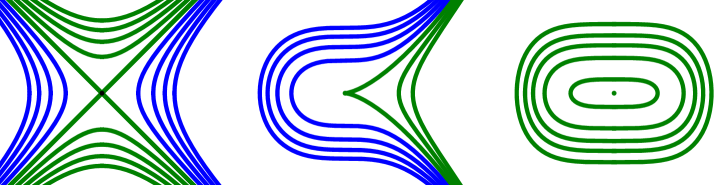
Figure 1: Level sets of $A_{k},\ k=1,2,3,$ singularities: $H=\xi^{2}-x^{2}$ (left), $H=\xi^{2}-x^{3}$ (middle), $H=\xi^{2}+x^{4}$ (right).

In this paper, we give a classification of such pairs $(H=\xi^{2}\pm x^{k},\omega)$ under local transformations preserving either the Hamiltonian $H$ or the corresponding fibration $\{H=h\}$, in the $C^{\infty}$-smooth and analytic categories. More precisely, the group $\textup{Diff}(\mathbb{R}^{2},0)$ of local ($C^{\infty}$-smooth, respectively analytic) diffeomorphism germs at the origin acts on pairs $(H,\omega)$ by taking the pull-back:

$$(\psi^{*}H,\psi^{*}\omega),\quad\psi\in\textup{Diff}(\mathbb{R}^{2},0)\,.$$

In the $H$-preserving case, we consider two pairs $(H_{0},\omega_{0})$ and $(H_{1},\omega_{1})$ to be equivalent if they belong to the same orbit of $\textup{Diff}(\mathbb{R}^{2},0)$, and in the fibration preserving case we additionally allow transformations on the left, that is, we consider two pairs $(H_{0},\omega_{0})$ and $(H_{1},\omega_{1})$ to be equivalent if there exists $\tilde{H}_{1}$ that defines the same (singular) foliation as $H_{1}$ and $(H_{0},\omega_{0})$ and $(\tilde{H}_{1},\omega_{1})$ are in the same orbit of $\textup{Diff}(\mathbb{R}^{2},0)$.

The main interest in this classification comes from the fact that $A_{k},\ k>1,$ singularities represent one of the simplest examples of degenerate singularities of integrable Hamiltonian systems and in the case $k=2\ell-1,\ \ell>1,$ (and $H=\xi^{2}+x^{2\ell}$), the action variable and the corresponding integer-affine structure do not suffice for their symplectic classification. Specifically, this means that there exist germs of symplectic structures $\omega_{0}$ and $\omega_{1}$ near the origin such that the pairs $(H=\xi^{2}+x^{2\ell},\omega_{0})$ and $(H=\xi^{2}+x^{2\ell},\omega_{1})$ with $\ell\geqslant 2$ have the same actions: for all $h>0$ sufficiently small,

$$I_{0}(h)=\int_{\{H\leqslant h\}}\omega_{0}=\int_{\{H\leqslant h\}}\omega_{1}=I_{1}(h),$$

while there exists no diffeomorphism germ preserving the fibration $\{H=h\}$ and sending $\omega_{1}$ to $\omega_{0}$. This observation is in striking contrast with essentially all of the local singularities for which the symplectic classification is currently known, including the $A_{1}$ singularity [9], more general elliptic and focus-focus singularities [15, 16, 30, 36], and also the $A_{2}$ singularity [4, 25], all of which typically occur in 2 or 3 degree of freedom integrable systems, see for instance [37, 7, 39, 3, 12, 14, 10, 6, 22]. This is also in contrast with most of the known global classifications provided the singularities are simple and non-splittable [11, 32, 33, 24, 27]. See also the works  [13, 40, 38, 3, 20, 34, 29, 23, 10, 7, 6, 5, 28, 2] for general classification problems of integrable systems.

One particular implication of the insufficiency of the action variable is that it is currently unknown whether the symplectic invariants of the Hamiltonian system

$$(H=\xi^{2}+x^{2\ell}+O(\|(x,\xi)\|^{2\ell+1}),\textup{d}\xi\wedge\textup{d}x),\ \ell\geqslant 2,$$

near the origin are spectrally determined: the usual (second order) Bohr-Sommerfeld rules allow one to reconstruct only the action variables from the spectrum of the Weyl quantisation $\hat{H}$ of $H$; this suffices in the elliptic case [35], but already not so in the quartic situation.

All this naturally gives rise to the questions of

• what extra symplectic invariants (apart from the action variable) exist?

• what are the symplectic normal forms (up to transformations preserving $H$ or, resp., the fibration induced by $H$)?

• does the spectrum of the Weyl quantisation $\hat{H}$ still contain all the information about the symplectic invariants?

In this work, we present a complete solution to the first two of these questions. In particular, we show that $(H=\xi^{2}\pm x^{k},\omega)$ can be brought to a normal form

$$\big{(}H=\xi^{2}\pm x^{k},\omega=\sum_{i=0}^{k-2}x^{i}c_{i}(H)\big{)},$$

where $c_{i}$ is unique up to certain (explicitly given) relations, which depend on the type of classification ($H$-preserving or fibration-preserving), the parity of $k$, and the sign in the Hamiltonian $H=\xi^{2}\pm x^{k}$ as well as the smoothness class: $C^{\infty}$-smooth or real-analytic. The functions $c_{i}$ taken up to these relations form a complete and minimal set of symplectic invariants, in the sense that two pairs $(H=\xi^{2}\pm x^{k},\omega_{0})$ and $(H=\xi^{2}\pm x^{k},\omega_{1})$ have the same invariants if and only if they are equivalent (in their respective regularity class) up to

• $H$-preserving diffeomorphisms, that is, are in the same orbit of $\textup{Diff}(\mathbb{R}^{2},0)$, or, respectively,

• fibration-preserving diffeomorphisms, that is, there exists a Hamiltonian $\tilde{H}$ defining the same (singular) foliation as $H$ such that $(H,\omega_{0})$ and $(\tilde{H},\omega_{1})$ are in the same orbit of $\textup{Diff}(\mathbb{R}^{2},0)$.

We note that in the complex-analytic category, these results are essentially known [17, 18]. What was missing is a real symplectic classification, especially in the $C^{\infty}$-smooth category, and the present paper is meant to fill in this gap; see also Theorems 3.1 and  4.4 below.

For example, for $k=4$ and $H=\xi^{2}+x^{4}$, the germs of $c_{0}$ and $c_{2}$ and the Taylor series of $\pm c_{1}$ at the origin (i.e., taken up to sign) classify the symplectic structures up to $H$-preserving $C^{\infty}$-smooth diffeomorphisms. The germs $c_{0}=c_{0}(H)$ and $c_{2}=c_{2}(H)$ correspond to the action variable, and in the fibration preserving case, $c_{0}$ can be set to one. The Taylor series of $c_{1}$ (taken up to sign) is an additional symplectic invariant that is not captured by the action variable. See Sections 3 and 4 for more detail.

One application of our results states that for $A_{k}$ singularities, there exists a canonical change of coordinates such that the Hamiltonian function still splits in the two variables at the cost of modifying the potential function:

Theorem 1.1.

Let $H\colon\mathbb{R}^{2}\to\mathbb{R}$ have an $A_{k}$ singularity at the origin. Then there exists a smooth (in the real-analytic case, real-analytic) local diffeomorphism $\varphi:(\mathbb{R}^{2},0)\to(\mathbb{R}^{2},0)$ preserving the canonical symplectic structure on $\mathbb{R}^{2}$ such that

$$H\circ\varphi=\tilde{\xi}^{2}+V(\tilde{x}),$$

for some smooth (in the real-analytic case, real-analytic) function $V$.

Interestingly, this shows that the familiar energy from classical mechanics (kinetic plus potential energy) turns out to be a universal model for all 1D Hamiltonians near an $A_{k}$ singularity.

Proof of Theorem 1.1.

The proof follows from Theorem 4.4 below. Indeed, according to this theorem, there exist (generally non-canonical) coordinates $(x,\xi)$ on $\mathbb{R}^{2}$ near the origin such that

$$H=\xi^{2}\pm x^{k+1},\quad k\geqslant 1,$$

and the symplectic structure has the form $\omega=\textup{d}(f\textup{d}\xi)$ for some $C^{\infty}$-smooth function $f=f(x)$ with $f^{\prime}(0)\neq 0$. Consider the change of variables $\tilde{\xi}=-\xi,\ \tilde{x}=f(x)$. Then

$$H(\tilde{x},\tilde{\xi})=\tilde{\xi}^{2}+V(\tilde{x}),$$

where $V=\pm(f^{-1}(\tilde{x}))^{k+1},$ and $\omega=\textup{d}\tilde{\xi}\wedge\textup{d}\tilde{x}.$ ∎

The paper is organised as follows. In Section 2, we reduce the problem of symplectic classification to its infinitesimal counterpart, by determining which energy-preserving symplectomorphisms arise via the Moser path method. In the next Sections 3 and 4, we classify the $A_{k}$ singularities up to energy-preserving and fibration-preserving symplectic transformations. The paper is concluded with a brief discussion of the conjecture that all of the symplectic invariants of $A_{k}$ singularities are spectrally determined.

2 $H$-preserving isotopies and symplectic classification

Let $\omega_{0}$ and $\omega_{1},\ \omega_{1}/\omega_{0}>0,$ be two symplectic forms defined in a neighborhood of the origin $O$ in $\mathbb{R}^{2}$. Assume that $H$ has an isolated singularity at $O$, such as the $A_{k}$ singularity. The question that we will now address is: when does there exist a local diffeomorphism $\Phi$ such that $\Phi^{*}\omega_{1}=\omega_{0}$ and $H\circ\Phi=H$? (We will use this later also for symplectic classification up to fibration-preserving diffeomorphisms.)

2.1 Moser isotopies

A sufficient condition for the existence of such a diffeomorphism $\Phi$ is given by the following lemma, which is an adaptation of the classical Moser’s trick, and works both in the $C^{\infty}$ and analytic categories. Let $(\varphi_{t})_{t\in[0,1]}$ be an isotopy of diffeomorphisms. (In this paper, we always impose $\varphi_{0}=\textup{Id}$). We say that this isotopy is $H$-preserving when $\varphi_{t}^{*}H=H$ for all $t\in[0,1]$.

Lemma 2.1.

(See [17].) Suppose that there exists a smooth solution $u$ of the cohomological equation

$$\textup{d}H\wedge\textup{d}u=\omega_{1}-\omega_{0}.$$ (1)

Then there exists a local $H$-preserving isotopy of diffeomorphisms $\Phi_{t}$ such that $\Phi_{0}=\textup{Id}$ and $\Phi_{1}^{*}\omega_{1}=\omega_{0}$.

Proof.

Let $\omega_{t}=\omega_{0}+t(\omega_{1}-\omega_{0}),\ t\in[0,1]$. Since $\omega_{1}/\omega_{0}>0$, the 2-form $\omega_{t}$ is non-degenerate for all $t\in[0,1]$. Hence we may define a vector field $X_{t}$ by the formula

$$i_{X_{t}}\omega_{t}=u\,\textup{d}H.$$

The required diffeomorphism can then be defined by integrating this vector field $X_{t}$ from $0$ to $1$, that is, as the solution at $t=1$ of the equation

$$\frac{\textup{d}}{\textup{d}t}\Phi_{t}=X_{t}\circ\Phi_{t},\quad\Phi_{0}=\textup{id}.$$

Indeed, under the map $\Phi_{t}$, we have $\frac{\textup{d}}{\textup{d}t}(\Phi_{t}^{*}\omega_{t})=\Phi_{t}^{*}(\textup{d}i_{X_{t}}\omega_{t}+\frac{\textup{d}}{\textup{d}t}\omega_{t})=\Phi_{t}^{*}(\operatorname{d}\!{u}\wedge\operatorname{d}\!{H}+\omega_{1}-\omega_{0})=0$ and hence $\Phi_{1}^{*}\omega_{1}=\omega_{0}.$

By the construction, the time-dependent vector field $X_{t}$ satisfies $\operatorname{d}\!{H}(X_{t})=0$, and hence is always tangent to the level curves $H=h$, which implies that $\Phi_{t}$ leaves $H$ invariant. It follows that $\Phi_{t}$ is as required. ∎

An $H$-preserving isotopy of diffeomorphisms obtained by the above construction will be called “of Moser type”. The requirement (1) has a natural cohomological interpretation, as follows. Since in dimension 2, $\Omega^{2}=Z^{2}$ (i.e. all $2$-forms are closed), we have by the Poincaré lemma the following short exact sequence (on $\mathbb{R}^{2}$ or any ball around the origin)

$$\lx@xy@svg{\hbox{\raise 0.0pt\hbox{\kern 6.68056pt\hbox{\ignorespaces\ignorespaces\ignorespaces\hbox{\vtop{\kern 0.0pt\offinterlineskip\halign{\entry@#!@&&\entry@@#!@\cr&&&&\crcr}}}\ignorespaces{\hbox{\kern-6.68056pt\raise 0.0pt\hbox{\hbox{\kern 0.0pt\raise 0.0pt\hbox{\hbox{\kern 3.0pt\raise 0.0pt\hbox{$\textstyle{\mathbb{R}\ignorespaces\ignorespaces\ignorespaces\ignorespaces}$}}}}}}}\ignorespaces\ignorespaces\ignorespaces\ignorespaces{}{\hbox{\lx@xy@droprule}}\ignorespaces{\hbox{\kern 30.68056pt\raise 0.0pt\hbox{\hbox{\kern 0.0pt\raise 0.0pt\hbox{\lx@xy@tip{1}\lx@xy@tip{-1}}}}}}{\hbox{\lx@xy@droprule}}{\hbox{\lx@xy@droprule}}{\hbox{\kern 30.68056pt\raise 0.0pt\hbox{\hbox{\kern 0.0pt\raise 0.0pt\hbox{\hbox{\kern 3.0pt\raise 0.0pt\hbox{$\textstyle{\Omega^{0}\ignorespaces\ignorespaces\ignorespaces\ignorespaces}$}}}}}}}\ignorespaces\ignorespaces\ignorespaces\ignorespaces{}{\hbox{\lx@xy@droprule}}\ignorespaces\ignorespaces\ignorespaces{\hbox{\kern 54.59164pt\raise 5.43056pt\hbox{{}\hbox{\kern 0.0pt\raise 0.0pt\hbox{\hbox{\kern 3.0pt\hbox{\hbox{\kern 0.0pt\raise-2.43056pt\hbox{$\scriptstyle{\operatorname{d}\!{}}$}}}\kern 3.0pt}}}}}}\ignorespaces{\hbox{\kern 70.70277pt\raise 0.0pt\hbox{\hbox{\kern 0.0pt\raise 0.0pt\hbox{\lx@xy@tip{1}\lx@xy@tip{-1}}}}}}{\hbox{\lx@xy@droprule}}{\hbox{\lx@xy@droprule}}{\hbox{\kern 70.70277pt\raise 0.0pt\hbox{\hbox{\kern 0.0pt\raise 0.0pt\hbox{\hbox{\kern 3.0pt\raise 0.0pt\hbox{$\textstyle{\Omega^{1}\ignorespaces\ignorespaces\ignorespaces\ignorespaces}$}}}}}}}\ignorespaces\ignorespaces\ignorespaces\ignorespaces{}{\hbox{\lx@xy@droprule}}\ignorespaces\ignorespaces\ignorespaces{\hbox{\kern 94.69373pt\raise 5.43056pt\hbox{{}\hbox{\kern 0.0pt\raise 0.0pt\hbox{\hbox{\kern 3.0pt\hbox{\hbox{\kern 0.0pt\raise-2.43056pt\hbox{$\scriptstyle{\operatorname{d}\!{}}$}}}\kern 3.0pt}}}}}}\ignorespaces{\hbox{\kern 110.72499pt\raise 0.0pt\hbox{\hbox{\kern 0.0pt\raise 0.0pt\hbox{\lx@xy@tip{1}\lx@xy@tip{-1}}}}}}{\hbox{\lx@xy@droprule}}{\hbox{\lx@xy@droprule}}{\hbox{\kern 110.72499pt\raise 0.0pt\hbox{\hbox{\kern 0.0pt\raise 0.0pt\hbox{\hbox{\kern 3.0pt\raise 0.0pt\hbox{$\textstyle{Z^{2}\ignorespaces\ignorespaces\ignorespaces\ignorespaces}$}}}}}}}\ignorespaces\ignorespaces\ignorespaces\ignorespaces{}{\hbox{\lx@xy@droprule}}\ignorespaces{\hbox{\kern 151.06667pt\raise 0.0pt\hbox{\hbox{\kern 0.0pt\raise 0.0pt\hbox{\lx@xy@tip{1}\lx@xy@tip{-1}}}}}}{\hbox{\lx@xy@droprule}}{\hbox{\lx@xy@droprule}}{\hbox{\kern 151.06667pt\raise 0.0pt\hbox{\hbox{\kern 0.0pt\raise 0.0pt\hbox{\hbox{\kern 3.0pt\raise 0.0pt\hbox{$\textstyle{0}$}}}}}}}\ignorespaces}}}}\ignorespaces\,, \textstyle{\mathbb{R}\ignorespaces\ignorespaces\ignorespaces\ignorespaces} \textstyle{\Omega^{0}\ignorespaces\ignorespaces\ignorespaces\ignorespaces} \scriptstyle{\operatorname{d}\!{}} \textstyle{\Omega^{1}\ignorespaces\ignorespaces\ignorespaces\ignorespaces} \scriptstyle{\operatorname{d}\!{}} \textstyle{Z^{2}\ignorespaces\ignorespaces\ignorespaces\ignorespaces} \textstyle{0} \textstyle{\mathbb{R}\ignorespaces\ignorespaces\ignorespaces\ignorespaces} \textstyle{\Omega^{0}\ignorespaces\ignorespaces\ignorespaces\ignorespaces} \scriptstyle{\operatorname{d}\!{}} \textstyle{\Omega^{1}\ignorespaces\ignorespaces\ignorespaces\ignorespaces} \scriptstyle{\operatorname{d}\!{}} \textstyle{Z^{2}\ignorespaces\ignorespaces\ignorespaces\ignorespaces} \textstyle{0}$$

giving the isomorphism $\delta:\frac{\Omega^{1}}{\operatorname{d}\!{\Omega^{0}}}\to Z^{2}$. The Moser method can be applied if we find a smooth $u$ such that $\omega_{1}-\omega_{0}=\operatorname{d}\!{H}\wedge\operatorname{d}\!{u}$, which is equivalent via $\delta^{-1}$ to $\alpha_{0}-\alpha_{1}=u\operatorname{d}\!{H}+\operatorname{d}\!{f}$, for some smooth function $f$, where $\alpha_{j}$ is a primitive of $\omega_{j}$; in other words, if $\delta^{-1}(\omega_{1}-\omega_{0})\in\Omega^{0}\operatorname{d}\!{H}+\operatorname{d}\!{\Omega_{0}}$. Therefore, we naturally introduce the “deformation space”

$$\mathcal{H}_{H}:=\frac{\Omega^{1}}{\Omega^{0}\operatorname{d}\!{H}+\operatorname{d}\!{\Omega_{0}}}\simeq\frac{Z^{2}}{\operatorname{d}\!{\Omega^{0}}\wedge\operatorname{d}\!{H}}$$

(sometimes called the vanishing cohomology, see [7]), and denote by $[\omega_{1}-\omega_{0}]_{H}$ the class of $\delta^{-1}(\omega_{1}-\omega_{0})$ in $\mathcal{H}_{H}$. Condition (1) is $[\omega_{1}-\omega_{0}]_{H}=0$. It turns out that, in the case of an $A_{k}$ singularity, there is a converse statement.

Proposition 2.2.

Let $\omega_{0}$, $\omega_{1}$ be symplectic forms near $0\in\mathbb{R}^{2}$. Let $H(x,\xi)=\xi^{2}\pm x^{k}$, $k\geqslant 2$. Then, there exists an $H$-preserving isotopy of diffeomorphisms $\Psi_{t}$ such that $\Psi_{0}=\textup{Id}$ and $\Psi_{1}^{*}\omega_{1}=\omega_{0}$ if and only if $[\omega_{1}-\omega_{0}]_{H}=0$. In this case, there exists an isotopy of Moser type with the same property.

Proof.

The last sentence is merely Lemma 2.1; hence we need to prove that the existence of the isotopy $\Psi_{t}$ (not necessarily of Moser type) implies the cohomological equation $[\omega_{1}-\omega_{0}]_{H}=0$. Let $\omega_{t}=(\Psi_{t}^{-1})^{*}\omega_{0}$ and let $\mathcal{X}_{H}^{t}$ be minus the Hamiltonian vector field of $H$ for the $\omega_{t}$ symplectic form, i.e.

$$i_{\mathcal{X}_{H}^{t}}\omega_{t}=\operatorname{d}\!{H}\,.$$ (2)

Let $X_{t}$ be the vector field of the isotopy, that is

$$X_{t}(\Psi_{t})=\frac{\operatorname{d}\!{\Psi_{t}}}{\operatorname{d}\!{t}}\,.$$

Since $\Psi_{t}$ preserves $H$ we must have $\operatorname{d}\!{H}(X_{t})=0$, which from (2) gives $\omega_{t}(\mathcal{X}_{H}^{t},X_{t})=0$. Hence $X_{t}$ is symplectically orthogonal to $\mathcal{X}_{H}^{t}$ which implies, by dimension consideration, that these vector fields must be collinear: there is a function $u_{t}$ such that

$$X_{t}=u_{t}\mathcal{X}_{H}^{t}.$$

Let us prove that $u_{t}$ must be smooth. Indeed, we have that $X_{t}$ is smooth as a function of $(x,\xi)$ for every $t$. Let $\omega_{t}=g(x,\xi,t)\operatorname{d}\!{\xi}\wedge\operatorname{d}\!{x}.$ Then $\mathcal{X}_{H}^{t}=(-2\xi,\pm kx^{k-1})/g$. Hence $(-2\xi u_{t},\pm kx^{k-1}u_{t})=X_{t}g$ and therefore also $(\xi u_{t},x^{k-1}u_{t})$ are smooth vector fields. Suppose $u_{t}$ is not smooth. Then the Taylor expansion of $\xi u_{t}$ at the origin (we only need to check smoothness at the origin) contains a non-zero term of the form $cx^{m}$. But then the Taylor expansion of $x^{k-1}u_{t}=(x^{k-1}/\xi)\xi u_{t}$ contains a non-zero term $cx^{m+k-1}/\xi,$ which implies $c=0$. This is a contradiction showing $u_{t}$ is smooth as a function of $(x,\xi)$ for every $t$.

Since $\Psi_{t}^{*}\omega_{t}=\omega_{0}$, we have

$$0=\frac{\operatorname{d}\!{}}{\operatorname{d}\!{t}}\Psi_{t}^{*}\omega_{t} =\Psi_{t}^{*}\left(\mathcal{L}_{X_{t}}\omega_{t}+\frac{\operatorname{d}\!{\omega_{t}}}{\operatorname{d}\!{t}}\right)$$ (3)

$$=\Psi_{t}^{*}\left(\operatorname{d}\!{(}i_{X_{t}}\omega_{t})+\frac{\operatorname{d}\!{\omega_{t}}}{\operatorname{d}\!{t}}\right)$$ (4)

$$=\Psi_{t}^{*}\left(\operatorname{d}\!{u}_{t}\wedge\operatorname{d}\!{H}+\frac{\operatorname{d}\!{\omega_{t}}}{\operatorname{d}\!{t}}\right)$$ (5)

and hence

$$\operatorname{d}\!{H}\wedge\operatorname{d}\!{u}_{t}=\frac{\operatorname{d}\!{\omega_{t}}}{\operatorname{d}\!{t}}.$$

Integrating over $[0,1]$, we see that the function $u:=\int_{0}^{1}u_{t}\operatorname{d}\!{t}$ satisfies our cohomological equation

$$\operatorname{d}\!{H}\wedge\operatorname{d}\!{u}=\omega_{1}-\omega_{0}\,,\quad\text{ \emph{i.e.} }\quad[\omega_{1}-\omega_{0}]_{H}=0\,.$$

The result follows (since by Lemma 2.1, there is an $H$-preserving isotopy $\Phi_{t}$ of Moser type such that $\Phi_{1}^{*}\omega_{1}=\omega_{0}$). ∎

2.2 $H$-preserving diffeomorphisms vs $H$-preserving isotopies

Let $H(x,\xi)=\xi^{2}\pm x^{k}$, with $k\geqslant 3$. Before we proceed to the symplectic classification, we need to know which $H$-preserving diffeomorphisms of an $A_{k}$ singularity arise as $H$-preserving isotopies. The following result is in contrast with the usual Morse case $k=2$.

Lemma 2.3.

Let $H(x,\xi)=\xi^{2}\pm x^{k}$, with $k\geqslant 3,$ and $\varphi$ be a $C^{\infty}$-smooth (respectively, real-analytic) diffeomorphism fixing the origin and such that $\varphi^{*}H=H$. Then there exists $\epsilon_{1}=\pm 1$, $\epsilon_{2}=\pm 1$ (with $\epsilon_{1}^{k}=1$), and $b\in\mathbb{R}$ such that the linear part of $\varphi,$ in coordinates $(x,\xi)$, is

$$\operatorname{d}\!{\varphi}(0)=\begin{pmatrix}\epsilon_{1}&b\\ 0&\epsilon_{2}\end{pmatrix}.$$

Let $A:=\begin{pmatrix}\epsilon_{1}&0\\ 0&\epsilon_{2}\end{pmatrix}$. Then, the map $\tilde{\varphi}:=\varphi\circ A$ preserves $H$ and is homotopic to the identity through a $C^{\infty}$-smooth (in the real-analytic case, real-analytic) $H$-preserving isotopy.

Proof.

We denote $\varphi(x,\xi)=(\varphi_{x}(x,\xi),\,\varphi_{\xi}(x,\xi))$, and $\operatorname{d}\!{\varphi}(0)=:\begin{pmatrix}a&b\\ c&d\end{pmatrix}$. We denote by $\mathcal{O}(k)$ the ideal of smooth functions on $\mathbb{R}^{2}$ whose Taylor series at the origin starts with a homogeneous polynomial in $(x,\xi)$ of degree $\geqslant k$. Writing

$$\varphi_{\xi}^{2}\pm\varphi_{x}^{k}=\xi^{2}\pm x^{k},$$ (6)

and using that $\varphi_{x}^{k}\in\mathcal{O}(k)$ we get

$$\varphi_{\xi}^{2}=\xi^{2}+\mathcal{O}(k).$$ (7)

Since $\varphi_{\xi}(x,\xi)^{2}=(cx+d\xi)^{2}+\mathcal{O}(3)$ and $k\geqslant 3$, we obtain, identifying coefficients, that $c=0$ and $d^{2}=1$. Hence $\varphi_{\xi}(x,\xi)=d\xi+\mathcal{O}(2)$, $d=\pm 1$. The full Taylor expansion of $\varphi_{\xi}$ is

$$\varphi_{\xi}(x,\xi)=d\xi+A_{2}+A_{3}+\cdots$$

where $A_{j}$ is homogeneous of degree $j$. Let $j_{0}\geqslant 2$ be the smallest index for which $A_{j_{0}}\neq 0$. Then the term of smallest degree in $\varphi_{\xi}^{2}-\xi^{2}$ is $2d\xi A_{j_{0}}$, of degree $j_{0}+1$. From (7) we deduce that $j_{0}+1\geqslant k$. Hence we have

$$\varphi_{\xi}(x,\xi)=d\xi+\mathcal{O}(k-1),\quad d=\pm 1,$$ (8)

and $\varphi_{\xi}^{2}=\xi^{2}+2d\xi A_{k-1}+\mathcal{O}(k+1)$. Writing now

$$\varphi_{x}(x,\xi)=ax+b\xi+S_{2}(x,\xi),$$ (9)

where $S_{2}\in\mathcal{O}(2)$, we have

$$\varphi_{x}(x,\xi)^{k}=(ax+b\xi)^{k}+\mathcal{O}(k+1)=(ax)^{k}+\xi D_{k-1}+\mathcal{O}(k+1)$$

where $D_{k-1}$ is homogeneous of degree $k-1$. From (6), we obtain

$$\pm(ax)^{k}\pm\xi D_{k-1}+\xi^{2}+2d\xi A_{k-1}=\pm x^{k}+\xi^{2}+\mathcal{O}(k+1),$$

which implies $a^{k}=1$, and $\pm D_{k-1}+2dA_{k-1}=0$.

For each $t>0$, consider the maps $h_{t}(x,\xi)=(t^{2}x,t^{k}\xi)$, and

$$\varphi_{t}(x,\xi)=\left(\frac{1}{t^{2}}\varphi_{x}(h_{t}(x,\xi)),\,\frac{1}{t^{k}}\varphi_{\xi}(h_{t}(x,\xi))\right)\,.$$ (10)

Observe that, from (8) and (9),

$$\varphi_{t}(x,\xi)=\left(ax+bt^{k-2}\xi+\frac{1}{t^{2}}S_{2}(t^{2}x,t^{k}\xi),\,d\xi+\frac{1}{t^{k}}B_{k-1}(t^{2}x,t^{k}\xi)\right)\,,$$

where $B_{k-1}\in\mathcal{O}(k-1)$. It follows that $\varphi_{t}$ is smooth with respect to all variables (including the case $t=0$) and converges to the linear map $\varphi_{0}(x,\xi)=(ax,d\xi)$ as $t\to 0$.

To conclude, we let $\epsilon_{1}:=a$, $\epsilon_{2}:=d$, and we see that $\varphi_{t}\circ A$ is the required isotopy. Indeed, we have already shown that $\varphi_{t}$ and hence $\varphi_{t}\circ A$ is smooth. Furthermore, $\varphi_{0}\circ A$ is the identity. Finally, notice that

$$\varphi_{t}^{*}H =\frac{1}{t^{2k}}\varphi_{\xi}^{2}\circ h_{t}\pm\frac{1}{t^{2k}}\varphi_{x}^{k}\circ h_{t}$$ (11)

$$=\frac{1}{t^{2k}}(\varphi^{*}H)\circ h_{t}$$ (12)

$$=\frac{1}{t^{2k}}H\circ h_{t}=H\,.$$ (13)

This shows that the isotopy preserves $H$. ∎

Remark 2.4.

In case when $\varphi$ preserves the ‘canonical’ symplectic structure $\operatorname{d}\!{\xi}\wedge\operatorname{d}\!{x}$, then so does the isotopy (10): $\varphi_{t}^{*}(\operatorname{d}\!{\xi}\wedge\operatorname{d}\!{x})=\operatorname{d}\!{\xi}\wedge\operatorname{d}\!{x}$ for all $t\in[0,1]$.

The following theorem will not be directly used in what follows, but can be proven by the same method.

Theorem 2.5.

Let $\omega$ be a symplectic structure around the origin in $\mathbb{R}^{2}$ and $\varphi$ be a $C^{\infty}$-smooth (respectively, real-analytic) diffeomorphism fixing the origin such that $\varphi^{*}\omega=\omega$ and $H\circ\varphi=H$, where $H=\xi^{2}\pm x^{k},\ k>2.$ Moreover, let $\textup{Inv}\colon\mathbb{R}^{2}\to\mathbb{R}^{2}$ be defined by $\textup{Inv}(x,\xi)=(-x,-\xi).$ If $k=2\ell+1$ is odd, then $\varphi$ must be a time-one map of the flow of a function of $H$. If $k=2\ell$ is even either $\varphi$ or $\varphi\circ\textup{Inv}$ is a time-one map of the flow of a function that is constant on the connected components of $H.$

Remark 2.6.

In the case when $H=\xi^{2}+x^{2\ell}$, then $\varphi$ or $\varphi\circ\textup{Inv}$ is a time-one map of the flow of a function of $H,$ since the fibers $H^{-1}(h)$ are connected in this case. In the real-analytic case, $\varphi$ or $\varphi\circ\textup{Inv}$ is a time-one map of the flow of a function of $H$ also when $H=\xi^{2}-x^{2\ell}.$

Proof of Theorem 2.5.

By Lemma 2.3, we can without loss of generality assume that $\varphi$ is isotopic to the identity via a $C^{\infty}$-smooth (respectively, real-analytic) $H$-preserving isotopy. Let $\varphi_{t}$ be such an isotopy and $X_{t}$ its vector field, given by

$$X_{t}(\varphi_{t})=\frac{\operatorname{d}\!{\varphi_{t}}}{\operatorname{d}\!{t}}\,.$$

As in the proof of Proposition 2.2, we have that $X_{t}=u_{t}\mathcal{X}_{H}$ for a $C^{\infty}$-smooth (in the real-analytic case, real-analytic) function $u_{t}$, where $\mathcal{X}_{H}$ is minus the Hamiltonian vector field of $H.$ Moreover, the function $u:=\int_{0}^{1}u_{t}(\varphi_{t})$ satisfies the cohomological equation $\operatorname{d}\!{H}\wedge\operatorname{d}\!{u}=0\,$ since $\varphi=\varphi_{1}$ preserves $\omega$. In particular, $u$ is constant on the connected components of $H$. Then any smooth function $g$ such that $\operatorname{d}\!{g}=u\operatorname{d}\!{H}$ is as required. Indeed, let $B_{\varepsilon}\subset\mathbb{R}^{2}$ be a small open ball around the origin. Then on each connected component of $B_{\varepsilon}\setminus\{H=0\}$ we can write

$$\omega=\textup{d}H\wedge\textup{d}V$$

for some variable $V$, which is multivalued when $H=\xi^{2}+x^{2\ell}$ and single-valued otherwise. (This is a simple version of the Darboux-Carathéodory theorem, which in this case directly follows from $\operatorname{d}\!{H}\neq 0$ outside $H=0$.) Observe that in the $(V,H)$ coordinates,

$$\frac{\operatorname{d}\!{\varphi_{t}}}{\operatorname{d}\!{t}}=u_{t}\mathcal{X}_{H}|_{\varphi_{t}}=\left(u_{t}(\varphi_{t}),0\right)$$

and hence

$$\varphi(1)-\varphi(0)=\int_{0}^{1}\left(u_{t}(\varphi_{t}),0\right)\textup{d}t=(u,0).$$

But the same is true for the time-one map of the flow of $\mathcal{X}_{g}$. The result follows. ∎

2.3 Symplectic classification

The preceding discussion shows that in order to reduce the pair $(H,\omega_{0})$ to a new, hopefully simpler pair $(H,\omega_{1})$, it essentially suffices to apply Lemma 2.1, i.e. find a smooth function $u$ solving the cohomological equation (1). Indeed, for any $H$-preserving symplectomorphism $\varphi$ with $\varphi^{*}\omega_{1}=\omega_{0},\,\omega_{1}/\omega_{0}>0,$ it holds that either $\varphi$ or $\varphi\circ\textup{Inv},$ where $\textup{Inv}(x,\xi)=(-x,-\xi),$ arises from an $H$-preserving isotopy of Moser type; see Proposition 2.2 and Lemma 2.3.

Observe that Eq. (1) is simply a linear PDE (a transport equation) on the unknown function $u$, for it can be rewritten as

$$\partial_{x}u\cdot\partial_{\xi}H-\partial_{\xi}u\cdot\partial_{x}H=g(x,\xi),$$ (14)

where

$$\omega_{1}-\omega_{0}=g(x,\xi)\textup{d}\xi\wedge\textup{d}x.$$

We note that Eq. (14) can always be formally solved, as shown below, but not always can one find a smooth (or even an everywhere well-defined) solution. Indeed, let us look for a solution of the form $u=\tilde{u}(\xi,H(x,\xi))$. We have $\operatorname{d}\!{H}\wedge\operatorname{d}\!{u}=-\partial_{\xi}\tilde{u}\partial_{x}H\operatorname{d}\!{\xi}\wedge\operatorname{d}\!{x}$. Hence, let $\varepsilon=\varepsilon(x,\xi)$ be a function that is constant on the connected components of the level sets of $H$. Then the following formula, coming from the initial condition $\tilde{u}|_{x=-\varepsilon(x,\xi)}=0$,

$$\tilde{u}(\xi,h)=\int_{-\varepsilon(x,\xi)}^{\xi}\dfrac{g(\beta(t,h),t)}{-\partial_{x}H(\beta(t,h),t)}\textup{d}t,\quad\text{ where }\ \ H(\beta(t,h),t)=t^{2}\pm\beta^{k}(t,h)=h,$$ (15)

gives rise to a solution $u=\tilde{u}(\xi,H(x,\xi))$ of Eq. (14); the general solution is then $\tilde{u}(\xi,H(x,\xi))+a(x,\xi)$, where $a=a(x,\xi)$ is constant on the connected components of the levels sets of $H$.

We will use these observations in the following way. We start with local coordinates $(x,\xi)$ around the origin in $\mathbb{R}^{2}$ in which the Hamiltonian

$$H(x,\xi)=\xi^{2}\pm x^{k},$$

but the symplectic structure $\omega_{0}=g_{0}(x,\xi)\textup{d}\xi\wedge\textup{d}x$ is arbitrary. Then we will bring the symplectic structure to the form $\omega_{0}=\omega_{norm}+\textup{d}H\wedge\textup{d}u$, where $\omega_{norm}$ is in normal form giving (possibly modulo the action of the involution $\textup{Inv}(x,\xi)=(-x,-\xi)$) the desired symplectic invariant of the $H$-preserving symplectic equivalence. Finally, the normal form $\omega_{norm}$ will be simplified further by allowing ‘transformations on the left’, resulting in the normal form of the fibration $H\colon\mathbb{R}^{2}\to\mathbb{R}$ near the origin.

The idea behind the procedure goes back to [9]; see also [17, 18, 19] and the more recent works [4] and [25] very close to this point of view. The procedure is general and can in theory be applied to any Hamiltonian function. In this paper, we restrict our attention to Hamiltonians having an isolated singularity of the type $A_{k}$, which is a simplest (possibly) degenerate singularity in one dimension.

Note that so far the discussion in the smooth and real-analytic categories has been completely parallel. The precise results and the proofs however will be somewhat different in these two cases. In what follows, the two cases are hence considered separately.

3 Symplectic classification in the real-analytic case

Let $H$ be a real-analytic Hamiltonian on $(\mathbb{R}^{2},\omega)$ with an $A_{k-1},k\geqslant 2,$ singularity at the origin $O$. The following result gives a local symplectic classification of $(H,\omega)$ near $O$ up to $H$-preserving real-analytic diffeomorphism germs, as defined in the Introduction.

Theorem 3.1.

Let $H$ be a real-analytic Hamiltonian on $(\mathbb{R}^{2},\omega)$ having $A_{k-1},k\geqslant 2,$ singularity at the origin $O$. Then the pair $(H,\omega)$ has the following local symplectic normal form near $O$ for the group of $H$-preserving real-analytic diffeomorphism germs:

$$\big{(}H=\xi^{2}\pm x^{k},\ \omega=\textup{d}(f\textup{d}\xi)\big{)},\quad\mbox{ where }f=\sum_{i=1}^{k-1}x^{i}f_{i}(x^{k}),$$ (16)

for some real-analytic functions $f_{i}$ with $f_{1}(0)\neq 0$ defined uniquely modulo the following relation: if $k=2\ell$ is even, then $f$ is uniquely defined up to changing the sign of $\sum_{i=1}^{\ell-1}x^{2i}f_{2i}(x^{2\ell})$. In other words,

• if $k$ is odd, then (the Taylor series of) $f_{i},i=1,\ldots,k-1,$ form a complete and minimal set of symplectic invariants;

• if $k=2\ell$ is even, then (the Taylor series of) $f_{i},i=1,\ldots,k-1,$ form a complete set of symplectic invariants with the only relation given by changing the sign of $\sum_{i=1}^{\ell-1}x^{2i}f_{2i}(x^{2\ell})$.

Remark 3.2.

The ambiguity in the sign of $\sum_{i=1}^{\ell-1}x^{2i}f_{i}(x^{2\ell})$ comes from the following fact. If $k$ is even, the transformation $\textup{Inv}(x,\xi)=(-x,-\xi)$ is an $H$-preserving diffeomorphism that transforms the function $f(x)$ from Eq. (16) to $-f(-x)$. However, when $k=2\ell$ with $\ell\geqslant 2$, $\textup{Inv}(x,\xi)$ cannot be included into a smooth $H$-preserving flow and hence is not of Moser type: when $H=\xi^{2}-x^{2\ell}$ this follows since Inv swaps the connected components of the level sets of $H$; when $H=\xi^{2}+x^{2\ell},$ one can show that the ‘action variable’

$$I^{\prime}(h)/2=\int_{-\sqrt{h}}^{\sqrt{h}}\frac{\operatorname{d}\!{\xi}}{k(\xi^{2}-h)^{\frac{k-1}{k}}}=h^{\frac{1-\ell}{2\ell}}\int_{-1}^{1}\frac{\operatorname{d}\!{s}}{k(s^{2}-1)^{\frac{k-1}{k}}}$$

being singular for $\ell>1$ is an obstruction; see [26].

In the odd case, on the contrary, every $H$-preserving and orientation-preserving diffeomorphism is of Moser type by Proposition 2.2 and Lemma 2.3.

In order to prove Theorem 3.1, let us first show that one can achieve the normal form (16) by means of Moser isotopies, which, by Lemma 2.1 amounts to solving the cohomological equation

$$\operatorname{d}\!{H}\wedge\operatorname{d}\!{u}=(g(x,\xi)+f^{\prime}(x))\operatorname{d}\!{\xi}\wedge\operatorname{d}\!{x}\,,$$

for some smooth functions $u$ and $f$. In order to simplify notation, we identify $\Omega^{2}$ with $\Omega^{0}$ using the canonical symplectic form $\operatorname{d}\!{\xi}\wedge\operatorname{d}\!{x}$, and the corresponding Poisson bracket $\{\cdot,\cdot\}$. Hence the above equation now reads:

$$\{H,u\}=g(x,\xi)+f^{\prime}(x)\,.$$

Proposition 3.3.

Let $H=\xi^{2}\pm x^{k}$, $k\geqslant 2$. For any formal series $g(x,\xi)\in\mathbb{R}[\![x,\xi]\!]$ there exists a unique formal series of the form $c(x)=\sum_{i=0}^{k-2}x^{i}c_{i}(x^{k})$, $c_{i}\in\mathbb{R}[\![x]\!]$, for which the equation

$$\{H,u\}=g(x,\xi)-c(x)$$ (17)

admits a formal solution $u(x,\xi)$. Moreover, if $g$ is analytic at the origin $(0,0)\in\mathbb{R}^{2}$, then one can choose $u$ to be analytic at the origin, and hence all $c_{i}$’s are analytic at $x=0$.

Remark 3.4.

It will follow from the proof that the radius of convergence of $u$ and $c_{i}$ is at least $R/2$, where $R$ is the radius of convergence of $g$, see (28).

Proof of Proposition 3.3.

Step 1. First observe that without loss of generality, $g=g(x,\xi)$ is an even function of $\xi$. Indeed, let $g(x,\xi)=g_{0}(x,\xi^{2})+\xi g_{1}(x,\xi^{2})$. Then the function $\check{u}=\check{u}(x,\xi)$ given by

$$\check{u}(x,\xi)=\tilde{u}(x,\xi^{2}\pm x^{k}),\quad\tilde{u}(x,h)=\frac{1}{2}\int_{0}^{x}g_{1}(s,h\mp s^{k})ds,$$ (18)

is a well-defined formal series, which is convergent whenever $g$ is, and solves the cohomological equation

$$\{H,\check{u}\}=\xi g_{1}(x,\xi^{2})\,.$$ (19)

(Formula (18) is similar to (15) with the roles of $x$ and $\xi$ interchanged.) Now, (17) is equivalent to $\{H,u-\check{u}\}=g_{0}(x,\xi^{2})-c(x)$. In what follows, we will therefore replace $g(x,\xi)$ in (17) by $g(x,\xi^{2})$. Thus, consider the cohomological equation

$$\{H,u\}=s(x,\xi^{2})\,,$$ (20)

where $s=g(x,\xi^{2})-c(x)$ with $c=c(x)$ an unknown formal series to be determined.

Step 2. Take $u_{ij}=\frac{1}{2(i+1)}x^{i+1}\xi^{2j-1}$ with $i\geqslant 0,j\geqslant 1$. Then

$$\{H,u_{i,j}\}=x^{i}\xi^{2j}\mp\frac{(2j-1)k}{2(i+1)}x^{i+k}\xi^{2j-2}\,.$$

Hence summing up the monomials $u_{ij}=\frac{1}{2(i+1)}x^{i+1}\xi^{2j-1}$ with appropriate coefficients, one can eliminate the variable $\xi$ from the symplectic form, as follows. For notational convenience we introduce $\tau(i,j)=(i+k,j-1)$ and $h(i,j)=\frac{(2j-1)k}{2(i+1)}$, and denote $(x\xi)^{(i,j)}:=x^{i}\xi^{2j}$, so that the previous equation writes

$$\{H,u_{i,j}\}=(x\xi)^{(i,j)}\mp h(i,j)(x\xi)^{\tau(i,j)}\,.$$

Notice that the $j$-th iterate $(x\xi)^{\tau^{j}(i,j)}=x^{i+kj}$ depends only on $x$. Hence we may solve the equation

$$\{H,U_{i,j}\}=(x\xi)^{(i,j)}\mod\mathbb{R}[x]\qquad\text{(with }i\geqslant 0,j\geqslant 1\text{)}$$ (21)

using an Ansatz of the form

$$U_{i,j}=\sum_{n=0}^{j-1}a_{ij}^{n}u_{\tau^{n}(i,j)}\,.$$

In order to determine the coefficients $a_{ij}^{n}$ we write

$$\{H,U_{i,j}\} =\sum_{n=0}^{j-1}a_{ij}^{n}(x\xi)^{\tau^{n}(i,j)}\mp\sum_{n=0}^{j-1}a_{ij}^{n}h(\tau^{n}(i,j))(x\xi)^{\tau^{n+1}(i,j)}$$ (22)

$$=a_{ij}^{0}(x\xi)^{\tau^{0}(i,j)}+\sum_{n=1}^{j-1}\left(a_{ij}^{n}\mp a_{ij}^{n-1}h(\tau^{n-1}(i,j))\right)(x\xi)^{\tau^{n}(i,j)}$$ (23)

$$\quad\mp a_{ij}^{j-1}h(\tau^{j-1}(i,j))x^{i+kj}$$ (24)

in which the last term on the right belongs to $\mathbb{R}[x]$. Therefore (21) is satisfied if and only if

$$\begin{cases}a_{ij}^{0}=1\\ a_{ij}^{n}\mp a_{ij}^{n-1}h(\tau^{n-1}(i,j))=0\quad\text{ for }1\leqslant n\leqslant j-1\,,\end{cases}$$

which gives, for $1\leqslant n\leqslant j-1$,

$$a_{ij}^{n}=(\pm 1)^{n}\prod_{p=0}^{n-1}h(\tau^{p}(i,j))=(\pm 1)^{n}\frac{(2j-1)k}{2(i+1)}\frac{(2j-3)k}{2(i+1+k)}\cdots\frac{(2j-2n+1)k}{2(i+(n-1)k+1)}\,.$$

To summarize, we have obtained

$$\{H,U_{i,j}\} =(x\xi)^{(i,j)}\mp a_{ij}^{j-1}h(\tau^{j-1}(i,j))x^{i+kj}$$ (25)

$$=(x\xi)^{(i,j)}-(\pm 1)^{j}\prod_{p=0}^{j-1}h(\tau^{p}(i,j))x^{i+kj}\,.$$ (26)

Hence if we write

$$g(x,\xi^{2})=\sum_{0\leqslant i\atop 0\leqslant j}g_{i,j}(x\xi)^{(i,j)}$$

we can solve (20) formally by

$$u:=\sum_{i,j}g_{i,j}U_{i,j}=\sum_{i,j}\sum_{n=0}^{j-1}g_{i,j}a_{ij}^{n}u_{\tau^{n}(i,j)}\,.$$

For a fixed value $(\tilde{\imath},\tilde{\jmath})$ of $\tau^{n}(i,j)=(i+nk,j-n)$ there are only a finite number of relevant indices $n$, namely $0\leqslant n\leqslant\lfloor\frac{\tilde{\imath}}{k}\rfloor$. Therefore we can write

$$u=\sum_{\tilde{\imath},\tilde{\jmath}}\sum_{n=0}^{\lfloor\frac{\tilde{\imath}}{k}\rfloor}g_{i,j}a_{ij}^{n}u_{(\tilde{\imath},\tilde{\jmath})},\quad\mbox{ where }\ \ (i,j)=\tau^{-n}(\tilde{\imath},\tilde{\jmath})=(\tilde{\imath}-nk,\tilde{\jmath}+n)\,.$$

Let us show that the summation leads to a real-analytic function $u$ (and hence $c$) solving (20). For this we need to show that there exist constants $C,R$ such that

$$\forall\tilde{\imath}\geqslant 0,\tilde{\jmath}\geqslant 0,\quad\left|\sum_{n=0}^{\lfloor\frac{\tilde{\imath}}{k}\rfloor}g_{i,j}a_{ij}^{n}\right|\leqslant CR^{\tilde{\imath}+\tilde{\jmath}}\,.$$

Since we already know that $\left|g_{i,j}\right|\leqslant cr^{i+j}\leqslant cr^{i+kj}=cr^{\tilde{\imath}+k\tilde{\jmath}}\leqslant c(r^{k})^{\tilde{\imath}+\tilde{\jmath}}$, it is enough to show that

$$\left|\sum_{n=0}^{\lfloor\frac{\tilde{\imath}}{k}\rfloor}a_{ij}^{n}\right|\leqslant CR^{\tilde{\imath}+\tilde{\jmath}}\,.$$ (27)

Let us denote $i^{\prime}=\frac{i+1}{k}$ and $j^{\prime}=\frac{2j-1}{2}$. We have

$$\left|a_{ij}^{n}\right|=\frac{j^{\prime}}{i^{\prime}}\frac{(j^{\prime}-1)}{(i^{\prime}+1)}\cdots\frac{(j^{\prime}-n+1)}{(i^{\prime}+n-1)}=\frac{\Gamma(j^{\prime}+1)}{\Gamma(j^{\prime}-n+1)}\frac{\Gamma(i^{\prime})}{\Gamma(i^{\prime}+n)}$$

which can be rewritten in terms of the beta function $B(x,y)=\frac{\Gamma(x)\Gamma(y)}{\Gamma(x+y)}$ as

$$\left|a_{ij}^{n}\right|=\frac{B(i^{\prime},j^{\prime}+1)}{B(i^{\prime}+n,j^{\prime}-n+1)}.$$

It is known that $\left|B(x,y)\right|\leqslant\pi$ for $x,y\geqslant 1$, see [31, 5.12.2], and that $\left|\frac{1}{B(\frac{x+y+1}{2},\frac{x-y+1}{2})}\right|\leqslant 2^{x-1}x$ for $x\geqslant 1$, see [31, 5.12.5]. This gives, for $i^{\prime},j^{\prime}\geqslant 1$

$$\left|a_{ij}^{n}\right|\leqslant 2^{i^{\prime}+j^{\prime}-1}(i^{\prime}+j^{\prime})\pi\leqslant CR^{i^{\prime}+j^{\prime}}$$ (28)

for suitable constants. Since $i^{\prime}+j^{\prime}$ is constant in the sum (27), we get that the sum is bounded by $(\lfloor\frac{\tilde{\imath}}{k}\rfloor+1)CR^{i^{\prime}+j^{\prime}}\leqslant\tilde{C}{\tilde{R}}^{\tilde{\imath}+\tilde{\jmath}}$ for suitable $\tilde{C},\tilde{R}$, which proves the analyticity of $u$.

Step 3. It remains to understand the freedom left to simplify the function $c=c(x)$. We may decompose the space $\Omega^{0}$ of analytic functions of $(x,\xi)$ as

$$\Omega^{0}=\mathbb{R}\{\xi\}\oplus x\Omega^{0}\,,$$ (29)

where $\mathbb{R}\{\xi\}$ denotes the space of real analytic functions of $\xi$. Since $u_{i,j}\in x\Omega^{0}$, the computation in Step 2 shows that the map $u\mapsto\{H,u\}$ is surjective from $x\Omega^{0}$ onto $\mathbb{R}\{x,\xi^{2}\}\mod\mathbb{R}\{x\}$. Let us show that

$$\{H,\cdot\}:x\Omega^{0}\to\mathbb{R}\{x,\xi^{2}\}/\mathbb{R}\{x\}$$ (30)

is actually an isomorphism. The equation $\{H,u\}\in\mathbb{R}\{x\}$ writes

$$2\xi\partial_{x}u\mp kx^{k-1}\partial_{\xi}u=c(x)$$

for some analytic function $c$. Let us write $u=x^{m}v$, $v\in\Omega^{0}$, where $m\geqslant 1$ is maximal (assuming $u\neq 0$). Plugging this Ansatz we see that $c$ must be divisible by $x^{m-1}$. Dividing the equation by $x^{m-1}$ we get

$$2\xi(mv+x\partial_{x}v)\mp kx^{k}\partial_{\xi}v=\tilde{c}(x)\,,\quad\tilde{c}\in\Omega^{0}\,,$$

which actually implies (taking $x=\xi=0$) that $\tilde{c}(0)=0$. Restricting to $x=0$ we get $2m\xi v(0,\xi)=0$ and hence $v(0,\xi)=0$ for all $\xi$, therefore $v=x\tilde{v}$, which contradicts the maximality of $m$. Therefore, $u=0$, which shows that $\{H,\cdot\}$ is indeed injective on $x\Omega^{0}$.

We may now turn to solutions to the cohomological equation $\{H,u\}=c(x)$. We decompose $u=u_{0}+u_{1}$ according to (29), so that our equation becomes

$$\{H,u_{1}\}=c(x)+\{u_{0},H\}\,.$$

As in Step 1, we can assume that $\{u_{0},H\}=\pm kx^{k-1}\partial_{\xi}u_{0}$ is even in $\xi$ (notice that the function $u$ in (18) belongs to $x\Omega^{0}$), which means that $u_{0}(\xi)=\sum_{j\geqslant 0}a_{j}\xi^{2j+1}$. By the isomorphism (30), each choice of $u_{0}$ leads to a unique solution $u_{1}$, and this solution must hence be given by the construction of Step 2. Namely, each monomial $\xi^{2j+1}$ gives by $\{H,\cdot\}$ a monomial of type $(x\xi)^{(k-1,j)}$ which is absorbed in a unique way by $U_{k-1,j}$ as in (21), leaving on the right-hand side a monomial in $\mathbb{R}\{x\}$ of the form given by the last term of (22), i.e. a constant times $(x\xi)^{\tau^{j}(k-1,j)}=x^{k-1+jk}$. Therefore by suitably choosing $u_{0}$ we may formally eliminate any series of the form

$$\sum_{j\geqslant 0}\tilde{a}_{j}x^{k-1+jk}=x^{k-1}\sum_{j\geqslant 0}\tilde{a}_{j}x^{jk}$$

and only such series. It is left to observe that if $x^{k-1}\tilde{c}(x^{k})$ is real-analytic, then we may choose $u$ to be given by the explicit formula (see (15))

$$u=\tilde{u}(\xi,H(x,\xi)),\quad\mbox{where }\ \tilde{u}(\xi,h)=\frac{\mp 1}{k}\int_{0}^{\xi}\tilde{c}(h-s^{2})\textup{d}s,$$ (31)

and hence to be real-analytic. ∎

Proof of Theorem 3.1.

By Proposition 3.3, using Moser isotopies, we can transform the symplectic structure to the following form:

$$\psi^{*}\omega=\sum_{i=0}^{k-2}x^{i}c_{i}(x^{k})\textup{d}\xi\wedge\textup{d}x=\operatorname{d}\!{(}f\textup{d}\xi),\ f=\sum_{i=1}^{k-1}x^{i}f_{i}(x^{k}).$$

According to Lemma 2.3 and Proposition 2.2, further simplification of the normal form is possible only by using linear transformations $A$; this is effective only when $k$ is even, in which case the even part of $f$ is defined up to sign. Indeed, in this case $\textup{Inv}(x,\xi)=(-x,-\xi)$ is an $H$-preserving diffeomorphism that is not of Moser type and $\textup{Inv}^{*}\psi^{*}\omega=\textup{d}(-f(-x)\textup{d}\xi)$.

The conclusion is that we have found exactly one representative for every orbit of the group of real-analytic diffeomorphism germs. The result follows. ∎

In a similar way, one can prove the following result, which is useful for the fiber-wise symplectic classification problem. See also [17, Theorem 4] (or [18, Theorem 2.7]) for the case of general isolated singularities of (complex-)analytic functions; our result can be viewed as a specification of this general theorem to $A_{k}$ singularities.

Theorem 3.5.

Let $H$ be a real-analytic Hamiltonian on $(\mathbb{R}^{2},\omega)$ having $A_{k-1},k\geqslant 2,$ singularity at the origin $O$. Then the pair $(H,\omega)$ has also the following local symplectic normal form near $O$ for the group of $H$-preserving real-analytic diffeomorphism germs:

$$\big{(}H=\xi^{2}\pm x^{k},\ \omega=\sum_{i=0}^{k-2}x^{i}\tilde{c}_{i}(H)\textup{d}\xi\wedge\textup{d}x\big{)}$$ (32)

for some real-analytic functions $\tilde{c}_{i}$ with $\tilde{c}_{0}(0)\neq 0$ defined uniquely up to simultaneously changing the sign of the functions $\tilde{c}_{2i+1}(H),\ i=0,\ldots,\ell-2,$ when $k=2\ell$ is even. In other words,

• if $k$ is odd, then (the Taylor series of) $\tilde{c}_{i},i=0,\ldots,k-2,$ form a complete and minimal set of symplectic invariants;

• if $k=2\ell$ is even, then (the Taylor series of) $\tilde{c}_{i},i=0,\ldots,k-2,$ form a complete set of symplectic invariants with the only relation given by changing the sign of $\sum_{i=0}^{\ell-2}x^{2i+1}\tilde{c}_{2i+1}(H)$.

Proof.

By Theorem 3.1, we can assume that $g=\sum_{i=0}^{k-2}x^{i}c_{i}(x^{k})$. We would like to solve the cohomological equation

$$\operatorname{d}\!{H}\wedge\operatorname{d}\!{u}=(g(x)-\tilde{c}(x,H))\textup{d}\xi\wedge\textup{d}x,\qquad\tilde{c}=\sum_{i=0}^{k-2}x^{i}\tilde{c}_{i}(H),$$ (33)

where $\tilde{c}_{i}=\tilde{c}_{i}(H)$ are real-analytic functions to be determined later. In terms of the Poisson bracket, equation (33) reads

$$\{H,u\}=g(x)-\tilde{c}(x,H)=\sum_{i=0}^{k-2}\sum_{j\geqslant 0}x^{i}(c_{ij}x^{jk}-\tilde{c}_{ij}H^{j}),$$ (34)

where $c_{i}=\sum_{j\geqslant 0}c_{ij}x^{jk}$ and $\tilde{c}_{i}=\sum_{j\geqslant 0}\tilde{c}_{ij}H^{j}$.

Recall that for $u_{ij}=\frac{1}{2(i+1)}x^{i+1}\xi^{2j-1}$ with $i\geqslant 0,j\geqslant 1$, we have that

$$\{H,u_{i,j}\}=x^{i}\xi^{2j}\mp\frac{(2j-1)k}{2(i+1)}x^{i+k}\xi^{2j-2}\,.$$ (35)

It follows that for every $i=0,\ldots,k-2,$ and $j\geqslant 0,$ there exists a polynomial $U_{ij}$ and a unique constant $b_{j},\ |b_{j}|\geqslant 1,$ such that

$$\{H,U_{ij}\}=b_{j}x^{i+jk}-x^{i}H^{j}\,.$$

Indeed, one has

$$x^{i}H^{j}=\sum_{n=0}^{j}(\pm 1)^{n}\binom{j}{n}(x\xi)^{\tau^{n}(i,j)}$$

and using (25) we see that each term in this sum will contribute to a coefficient of $x^{i+kj}$ of sign $(\pm 1)^{n}\times(\pm 1)^{j-n}=(\pm 1)^{j}$, independent of $n$.

Hence setting

$$U:=\sum_{i=0}^{k-2}\sum_{j\geqslant 0}\frac{c_{ij}}{b_{j}}U_{ij},$$

we get that

$$\{H,U\}=g(x)-\sum_{i=0}^{k-2}\sum_{j\geqslant 0}\frac{c_{ij}}{b_{j}}x^{i}H^{j}.$$

This shows that equations (33-34) can be solved formally. To show that (33-34) admits a real-analytic solution, one can estimate the coefficients of $U$ similarly to how this is done in the proof of Theorem 3.1. However, a simpler proof can be obtained as follows. First note that by Eq.(35), the constants $b_{j}$ are always such that $|b_{j}|\geqslant 1$. Hence the series

$$g=\sum_{i=0}^{k-2}\sum_{j\geqslant 0}c_{ij}x^{i+jk}$$

being convergent implies that so is the series

$$\tilde{c}(x,H)=\sum_{i=0}^{k-2}\sum_{j\geqslant 0}\tilde{c}_{ij}x^{i}H^{j},$$

where $\tilde{c}_{ij}=c_{ij}/b_{j}$. But Proposition 3.3 now implies that we can solve the cohomological equation

$$\{H,\tilde{U}\}=c(x)-\tilde{c}(x,H)\,,$$

where $c=c(x)$ is the unique normal form of Proposition 3.3, which is convergent. But, by the construction of $\tilde{c}$, the function $g$ solves the latter cohomological equation formally. Hence, by uniqueness, $c=g$.

Thus, $u=\tilde{U}(x,\xi)$ is an analytic function solving (33). The result follows. ∎

As a corollary, we get

Theorem 3.6.

Let $H$ be a real-analytic Hamiltonian on $(\mathbb{R}^{2},\omega)$ having $A_{k-1},k\geqslant 2,$ singularity at the origin $O$. Then under the fibration-preserving equivalence, the pair $(H,\omega)$ has the following local symplectic analytic normal form near $O$:

$$\big{(}H=\xi^{2}\pm x^{k},\ \omega=(1+\sum_{i=1}^{k-2}x^{i}\hat{c}_{i}(H))\textup{d}\xi\wedge\textup{d}x\big{)}$$ (36)

for some real-analytic functions $\hat{c}_{i}$ defined uniquely up to simultaneously changing the sign of the functions $\hat{c}_{2i+1}(H),\ i=0,\ldots,\ell-2,$ when $k=2\ell$ is even. In other words,

• if $k$ is odd, then (the Taylor series of) $\hat{c}_{i},i=1,\ldots,k-2,$ form a complete and minimal set of symplectic invariants;

• if $k=2\ell$ is even, then (the Taylor series of) $\hat{c}_{i},i=1,\ldots,k-2,$ form a complete set of symplectic invariants with the only relation given by changing the sign of $\sum_{i=0}^{\ell-2}x^{2i+1}\hat{c}_{2i+1}(H)$.

Proof.

Let $\tilde{H}$ be a real-analytic Hamiltonian defining the same (singular) foliation as $H$ near the origin. Then $\tilde{H}=h(H)$ for an analytic germ $h$ with $h^{\prime}(0)\neq 0.$ Equivalently, we can write $h=Hg(H)$ for an analytic germ $g$ with $g(0)\neq 0.$ The fibration-preserving classification can be obtained by simplifying the $H$-preserving normal of $(H,\omega)$ by declaring $(\tilde{H}=Hg(H),\omega)$ and $(H,\omega)$ to be equivalent. On the level of $H$-preserving normal forms, this can specifically be done as follows.

Assume (without loss of generality) that $g(0)>0$ and change the variables according to

$$\psi(x,\xi)=(\tilde{x},\tilde{\xi}),\quad\tilde{\xi}=\xi\sqrt{g(H)},\ \tilde{x}=x(g(H))^{1/k}.$$

Then $Hg(H)={\tilde{\xi}}^{2}\pm{\tilde{x}}^{k}$ and it follows that the pairs $(H,\omega)$ and $(H,\tilde{\omega}=(\psi^{-1})^{*}\omega)$ are equivalent under the fibration-preserving equivalence. In other words, the normal forms

$$(h(H)={\tilde{\xi}}^{2}\pm{\tilde{x}}^{k},\ \tilde{\omega}=\sum_{i=0}^{k-2}\tilde{x}^{i}\hat{c}_{i}(h(H))\textup{d}\tilde{\xi}\wedge\textup{d}\tilde{x})\quad\mbox{ and }\quad(H={\xi}^{2}\pm{x}^{k},\ \omega=\sum_{i=0}^{k-2}x^{i}c_{i}(H)\textup{d}\xi\wedge\textup{d}x),$$

where

$$c_{i}(H)=\hat{c}_{i}(h(H))g(H)^{\frac{i+1}{k}-\frac{1}{2}}(g(H)+g^{\prime}(H)H)=\hat{c}_{i}(h(H))g(H)^{\frac{i+1}{k}-\frac{1}{2}}h^{\prime}(H),$$ (37)

are equivalent under the fibration-preserving equivalence.

Note that by applying the orientation-reversing diffeomorphisms $(x,\xi)\mapsto(x,-\xi)$ if necessary, we can achieve that $\hat{c}_{0}(0)>0$. Then we can uniquely solve the equation

$$h^{\prime}(H)\,|h(H)|^{\frac{1}{k}-\frac{1}{2}}\hat{c}_{0}(h(H))=|H|^{\frac{1}{k}-\frac{1}{2}}$$ (38)

for $h$ with the condition $h(0)=0$, making $c_{0}(H)\equiv 1$. Indeed, Eq. (38) with the condition $h(0)=0$ is equivalent to the integral equation

$$\int_{0}^{h(H)}|h|^{\frac{1}{k}-\frac{1}{2}}\hat{c}_{0}(h)\textup{d}h=\int_{0}^{H}|H|^{\frac{1}{k}-\frac{1}{2}}\textup{d}H=\textup{sign}(H)\frac{2k}{2+k}|H|^{\frac{1}{k}+\frac{1}{2}},$$

which has the form $\textup{sign}(h)\,|h|^{\frac{1}{k}+\frac{1}{2}}f(h)=\textup{sign}(H)|H|^{\frac{1}{k}+\frac{1}{2}}$ for some smooth function $f=f(h)$ with $f(0)=\hat{c}_{0}(0)>0.$ Equivalently, we can write this equation as

$$h\hat{f}(h)-H=0,\quad\hat{f}=f(h)^{\frac{2k}{2+k}},\ \hat{f}(0)>0,$$

which admits a unique real-analytic solution $h=h(H)$ near the origin by the Implicit Function Theorem. The result follows. ∎

Remark 3.7.

Note that orientation-reversing diffeomorphisms (e.g. $\psi(x,\xi)=(x,-\xi)$) in Theorem 3.6 are allowed. If we restrict to orientation-preserving diffeomorphisms, then the normal form is given by

$$\big{(}H={\xi}^{2}\pm{x}^{k},\ \pm 1+\sum_{i=1}^{k-2}x^{i}\hat{c}_{i}(H)\big{)}\textup{d}\xi\wedge\textup{d}x),$$

where the sign is plus if $\textup{d}\xi\wedge\textup{d}x/\omega>0$ and minus if $\textup{d}\xi\wedge\textup{d}x/\omega<0$.

4 Symplectic classification in the $C^{\infty}$-smooth case

We shall see in this section that in the $C^{\infty}$-smooth case, the symplectic classification works qualitatively differently depending on whether $H$ is a proper map in a neighbourhood of the origin. It turns out that for the ‘compact’ $A_{2\ell-1}$ singularities for which $H$ can be written in the form

$$H=\xi^{2}+x^{2\ell},\ \ell>1,$$

the symplectic invariants are given by a collection of both function germs and Taylor series, whereas for ‘non-compact’ $A_{k}$ singularities — which can then be expressed as the isolated singularity of the Hamiltonian $H=\xi^{2}-x^{k},$ with $k$ arbitrary — the symplectic invariants may be expressed in terms of Taylor series only; see Theorems 4.4, 4.6 and 4.7 below.

In the latter case of $H=\xi^{2}-x^{k},$ we will need the following result.

Theorem 4.1.

Let $H=\xi^{2}-x^{k}$ with $k\geqslant 2$ and $\omega_{0}$ and $\omega_{1}$ be arbitrary symplectic forms near $0\in\mathbb{R}^{2}$. Assume that the corresponding local action variables are equal up to a $C^{\infty}$-smooth function $f$:

$$I_{0}(h):=\int\limits_{R(h)}\omega_{0}=I_{1}(h)-f(h):=\int\limits_{R(h)}\omega_{1}-f(h),$$

where the region $R(h)$ is enclosed by the level curves $H=0,$ $x=(\xi^{2}-h)^{1/k},\ h\leqslant 0,$ and $\xi=\pm\varepsilon;$ see Figure 2. Then there exists a local $C^{\infty}$-smooth $H$-preserving isotopy $\psi_{t}$ of Moser type, such that $\psi_{1}^{*}\omega_{1}=\omega_{0}\,.$

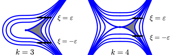
Figure 2: $H=\xi^{2}-x^{k}$ singularities for $k=3$ (left) and $k=4$ (right). The region $R(h)$ is shaded gray.

Proof.

The idea of the proof is to use the smoothness of (the derivative of) the difference of the local action variables

$$f^{\prime}(h)=\int_{-\varepsilon}^{\varepsilon}\frac{g((\xi^{2}-h)^{\frac{1}{k}},\xi)}{k(\xi^{2}-h)^{\frac{k-1}{k}}}\operatorname{d}\!{\xi}$$

to show the smoothness of the solution

$$u(x,\xi)=\tilde{u}(\xi,\xi^{2}-x^{k}),\quad\mbox{ where }\quad\tilde{u}(\xi,h)=\int^{\xi}_{-\varepsilon}\dfrac{g((t^{2}-h)^{1/k},t)}{k(t^{2}-h)^{\frac{k-1}{k}}}dt,$$ (39)

to the cohomological equation

$$\operatorname{d}\!{H}\wedge\operatorname{d}\!{u}=\omega_{1}-\omega_{0}=:g(x,\xi)\operatorname{d}\!{\xi}\wedge\operatorname{d}\!{x}.$$ (40)

This can be done similarly to the case of the cusp ($k=3$) singularity; see [25]. We give a complete proof in the Appendix. ∎

Remark 4.2.

We note that an analogous result is false for ‘compact’ $A_{2\ell-1}$ singularities $H=\xi^{2}+x^{2\ell}$ when $\ell\geqslant 2$: (the asymptotics of the) action variables do not suffice for their symplectic classification, neither in the $H$-preserving nor in the fibration preserving case. This follows from Theorems 4.4 and 4.7 below. As a concrete example, one can take

$$\big{(}H=\xi^{2}+x^{2\ell},\,\omega_{0}=\operatorname{d}\!{\xi}\wedge\operatorname{d}\!{x}\big{)}\quad\mbox{ and }\quad\big{(}H=\xi^{2}+x^{2\ell},\,\omega_{1}=(1+xc_{1}(x^{2\ell}))\operatorname{d}\!{\xi}\wedge\operatorname{d}\!{x}\big{)},$$

where $\ell\geqslant 2$ and $c_{1}$ is an arbitrary function whose Taylor series at the origin does not vanish identically. Equivalently, the following two integrable Hamiltonian systems

$$(H_{0}=\xi^{2}+x^{2\ell},\,\operatorname{d}\!{\xi}\wedge\operatorname{d}\!{x})\quad\mbox{ and }\quad(H_{1}=\xi^{2}+V(\tilde{x}),\,\operatorname{d}\!{\xi}\wedge\operatorname{d}\!{\tilde{x}}),$$

where the potential $V(\tilde{x})=x(\tilde{x})^{2\ell}$ for $\tilde{x}=x+f_{1}(x)$ with $f_{1}(x)=\int_{0}^{x}sc_{1}(s^{2\ell})\operatorname{d}\!{s}$ and $\ell\geqslant 2$, are not ($C^{\infty}$-smoothly or real-analytically) fiberwise symplectically equivalent even though their (real) action variables are identically the same.

To generalise the normal form results of the previous subsection to the $C^{\infty}$-smooth case, we will also need to find a $C^{\infty}$-smooth solution to a certain integral equation as in the following lemma:

Lemma 4.3.

Let $G\colon[0,h_{0}]\to\mathbb{R}$ be a $C^{\infty}$-smooth function on $[0,h_{0}],\,h_{0}>0,$ and $k\geqslant 2$ be a natural number. Then for each $i=0,1,\ldots,k-2$, the equation

$$\int_{-1}^{1}\dfrac{c_{i}(h(1-\xi^{2}))}{(1-\xi^{2})^{\frac{k-1-i}{k}}}\operatorname{d}\!{\xi}=G(h)$$

admit a $C^{\infty}$-smooth solution $c_{i}\in C^{\infty}([0,h_{0}])$ (with an “explicit” formula).

Proof.

Letting $u=1-\xi^{2}$ for $\xi\in[0,1]$ we obtain

$$\int_{-1}^{1}\frac{c_{i}(h(1-\xi^{2}))}{(1-\xi^{2})^{\frac{k-1-i}{k}}}\operatorname{d}\!{\xi}=\int_{0}^{1}\frac{c_{i}(hu)}{u^{\frac{k-1-i}{k}}}\frac{\operatorname{d}\!{u}}{\sqrt{1-u}}.$$

Introducing $\tilde{c}_{i}(t):=t^{\frac{i+1-k}{k}}c_{i}(t)$ and $\tilde{G}(h):=h^{\frac{i+1-k/2}{k}}G(h)$, our equation becomes

$$\int_{0}^{h}\frac{\tilde{c}_{i}(t)}{\sqrt{h-t}}\operatorname{d}\!{t}=\tilde{G}(h)\,.$$

We recognize the Abel transform. Since $\tilde{G}\in L^{1}(0;h_{0})$ we may write the inverse Abel transform [1] to obtain:

$$\tilde{c}_{i}(t)=\frac{1}{\pi}\frac{\operatorname{d}\!{}}{\operatorname{d}\!{t}}\int_{0}^{t}\frac{\tilde{G}(h)}{\sqrt{t-h}}\operatorname{d}\!{h}\,.$$

Note that the derivative of the integrand is not $L^{1}$, but we can write

$$\int_{0}^{t}\frac{\tilde{G}(h)}{\sqrt{t-h}}\operatorname{d}\!{h} =t^{1/2}\int_{0}^{1}\frac{\tilde{G}(tv)}{\sqrt{1-v}}\operatorname{d}\!{v}$$ (41)

$$=t^{\frac{i+1}{k}}\int_{0}^{1}v^{\frac{i+1-k/2}{k}}\frac{G(tv)}{\sqrt{1-v}}\operatorname{d}\!{v}\,,$$ (42)

in which form it is now licit to take the derivative under the integral sign. We have

$$\frac{\operatorname{d}\!{}}{\operatorname{d}\!{t}}\left(t^{\frac{i+1}{k}}\int_{0}^{1}v^{\frac{i+1-k/2}{k}}\frac{G(tv)}{\sqrt{1-v}}\operatorname{d}\!{v}\right)\\ =t^{\frac{i+1-k}{k}}\left(\frac{i+1}{k}\int_{0}^{1}v^{\frac{i+1-k/2}{k}}\frac{G(tv)}{\sqrt{1-v}}\operatorname{d}\!{v}+t\int_{0}^{1}v^{\frac{i+1+k/2}{k}}\frac{G^{\prime}(tv)}{\sqrt{1-v}}\operatorname{d}\!{v}\right).$$ (43)

Hence, we obtain

$$c_{i}(t)=t^{\frac{k-i-1}{k}}\tilde{c}_{i}(t)=\frac{1}{\pi}\left(\frac{i+1}{k}\int_{0}^{1}v^{\frac{i+1-k/2}{k}}\frac{G(tv)}{\sqrt{1-v}}\operatorname{d}\!{v}+t\int_{0}^{1}v^{\frac{i+1+k/2}{k}}\frac{G^{\prime}(tv)}{\sqrt{1-v}}\operatorname{d}\!{v}\right),$$

and we see that the right-hand side is smooth. ∎

We now turn to the right symplectic classification in the smooth category.

Theorem 4.4.

Let $H$ be a $C^{\infty}$-smooth Hamiltonian on $(\mathbb{R}^{2},\omega)$ having $A_{k-1},k\geqslant 2,$ singularity at the origin $O$. Then the pair $(H,\omega)$ has the following local symplectic normal form near $O$ for the group of $H$-preserving $C^{\infty}$-smooth diffeomorphism germs:

$$\big{(}H=\xi^{2}\pm x^{k},\ \omega=\textup{d}(f\textup{d}\xi)\big{)},\quad\mbox{ where }f=\sum_{i=1}^{k-1}x^{i}f_{i}(x^{k}),$$ (44)

for some $C^{\infty}$-smooth functions $f_{i}$ with $f_{1}(0)\neq 0$ defined uniquely modulo the following relations:

• if $k=2\ell+1$ is odd, then $f_{i}$’s are uniquely defined up to addition of flat functions (that is, the Taylor series of $f_{i}$’s form a complete and minimal set of symplectic invariants);

• if $k=2\ell$ is even and $H=\xi^{2}-x^{2\ell}$, then $f_{i}$’s are uniquely defined up to addition of flat functions and changing the sign of $\sum_{i=1}^{\ell-1}x^{2i}f_{2i}(x^{2\ell})$;

• if $k=2\ell$ is even and $H=\xi^{2}+x^{2\ell}$, the even-indexed functions $f_{2i},1\leqslant i\leqslant\ell-1,$ are uniquely defined up to addition of flat functions and changing the sign of $\sum_{i=1}^{\ell-1}x^{2i}f_{2i}(x^{2\ell})$.

Remark 4.5.

Thus, the only difference with the real-analytic case appears for $A_{2\ell-1}$ singularities given by $H=\xi^{2}+x^{2\ell},\ \ell\geqslant 1$, in which case these are the germs of the functions $f_{2i+1},0\leqslant i\leqslant\ell-1,$ rather than their Taylor series that are the symplectic invariants.

Proof.

Step 1.1. The first two cases ($k$ odd and $k=2\ell$ even with $H=\xi^{2}-x^{2\ell}$, respectively) follow from the analytic case using Borel summation and Theorem 4.1 above. Indeed, one can take $f=f(x)$ to be any smooth function such that its Taylor series at the origin gives the formal normal form for $\omega.$ Then $\omega_{0}=\textup{d}(f\textup{d}\xi)$ and $\omega_{1}=\omega$ satisfy the conditions of Theorem 4.1.

More specifically, we first observe that there exists a smooth function $u$ that solves the cohomological equation

$$\operatorname{d}\!{H}\wedge\operatorname{d}\!{u}=\omega_{1}-\omega_{0}\mod\quad\mathcal{O}(\infty)\operatorname{d}\!{\xi}\wedge\operatorname{d}\!{x},$$

i.e., up to a flat 2-form. This follows from the formal solution to this equation constructed in Theorem 3.1 by applying the Borel summation. Thus without loss of generality,

$$\omega_{1}-\omega_{0}=g(x,\xi)\operatorname{d}\!{\xi}\wedge\operatorname{d}\!{x},$$

where $g=g(x,\xi)$ is a $C^{\infty}$-smooth flat function germ at the origin. But then the corresponding ‘local’ action variables (see Theorem 4.1) satisfy

$$I_{1}(h)=I_{0}(h)+f(h),\quad f(h):=\int^{\varepsilon}_{-\varepsilon}\dfrac{g((t^{2}-h)^{1/k},t)}{k(t^{2}-h)^{\frac{k-1}{k}}}dt.$$

where $f=f(h)$ is $C^{\infty}$-smooth on $[-h_{0},0]$ with $h_{0}$ is sufficiently small: Indeed, since $g(x,\xi)$ is flat at the origin, we can write $g=x^{N}\tilde{g}(x,\xi)$ with $N$ arbitrary large. Then we see that

$$f(h)=\frac{1}{k}\int^{\varepsilon}_{-\varepsilon}(t^{2}-h)^{\frac{N+1-k}{k}}g((t^{2}-h)^{1/k},t)dt$$

is at least $C^{[\frac{N}{k}]-1}$-differentiable. Letting $N\to\infty$, we get that $f=f(h)$ is $C^{\infty}$-smooth. Hence we can apply Theorem 4.1.

Step 1.2. To conclude the proof in the case when $k$ is odd or $k=2\ell$ is even with $H=\xi^{2}-x^{2\ell}$, it is therefore left to show the uniqueness of the Taylor series of $f_{i}$ up to changing the sign of $\sum_{i=1}^{\ell-1}x^{2i}f_{2i}(x^{2\ell})$ when $k=2\ell$ is even. This follows from the proof in the analytic case by virtue of Lemma 2.3 and Proposition 2.2.

Step 2.1. In the remainder of the proof we consider the case of a ‘compact’ $A_{2\ell-1}$ singularity, i.e., the case when $k=2l$ and $H=\xi^{2}+x^{2l}.$ For simplicity, we shall assume that $H=\xi^{2}+x^{4}$ (the proof for larger $k=2\ell$ is similar).

Observe that without loss of generality, $g=g(x,\xi^{2})$ is an even function of $\xi$. Indeed, formula (18) works equally well in the smooth case. Let

$$g(x,\xi^{2})=g_{0}(x^{4},\xi^{2})+xg_{1}(x^{4},\xi^{2})+x^{2}g_{2}(x^{4},\xi^{2})+x^{3}g_{3}(x^{4},\xi^{2}).$$

We can similarly assume that $g_{3}\equiv 0$: letting

$$v=\tilde{v_{4}}(\xi,H(x,\xi)),\quad\mbox{where }\ \tilde{v}(\xi,h)=\frac{-1}{4}\int_{0}^{\xi}\tilde{g}_{3}(h-s^{2},s^{2})\textup{d}s,$$ (45)

we get that $\{H,v\}=x^{3}g_{3}(x^{4},\xi^{2}).$ Hence we can subtract this expression from $g$ using Lemma 2.1.

Now observe that one can find functions $c_{i}=c_{i}(x^{4}),0\leqslant i\leqslant 2,$ depending on $x$ only and such that

$$\int_{-h^{1/2}}^{h^{1/2}}\frac{c_{i}(h-\xi^{2})}{(h-\xi^{2})^{(3-i)/4}}\textup{d}\xi=\int_{-h^{1/2}}^{h^{1/2}}\frac{g_{i}(h-\xi^{2},\xi^{2})}{(h-\xi^{2})^{(3-i)/4}}\textup{d}\xi,$$ (46)

which is equivalent to

$$\int_{-1}^{1}\frac{c_{i}(h(1-\xi^{2}))}{(1-\xi^{2})^{(3-i)/4}}\textup{d}\xi=\int_{-1}^{1}\frac{g_{i}(h(1-\xi^{2}),h\xi^{2})}{(1-\xi^{2})^{(3-i)/4}}\textup{d}\xi.$$

The right-hand-side of the last equation is a smooth function of $h$ since $g$ is smooth; solving the integral equation produces a smooth solution $c_{i}$ by Lemma 4.3.

We would now like to show that there exists a smooth solution $u_{i}$ to the cohomological equation

$$\textup{d}H\wedge\textup{d}u=x^{i}(g_{i}(x^{4},\xi^{2})-c_{i}(x^{4}))\textup{d}\xi\wedge\textup{d}x.$$ (47)

Indeed, such an $u_{i}$ is given by

$$u_{i}(x,\xi)=\tilde{u_{i}}(\xi^{2}+x^{k},\xi),\quad\tilde{u_{i}}(h,\xi)=-\frac{1}{4}\int_{-\sqrt{h}}^{\xi}\dfrac{g_{i}(h-s^{2},s^{2})-c_{i}(h-s^{2})}{(h-s^{2})^{(3-i)/4}}ds,$$ (48)

which can be shown to be smooth by the construction of $c_{i}$; cf. [25]. Indeed, let $\alpha(x,\xi^{2})=x^{i}(g_{i}(x^{4},\xi^{2})-c_{i}(x^{4}))$. Then for an arbitrary large $n\in\mathbb{N}$, there exist $C^{\infty}$-smooth functions $R$ and $v$ such that

$$\alpha(x,\xi^{2})=\sum_{k=0}^{n}B_{k}x^{k}+x^{n+1}R(x,\xi^{2})+\textup{d}H\wedge\textup{d}v.$$ (49)

The proof of this is similar to the one used in the analytic case (see Step 2 of the proof of Theorem 4.1 for details). Recalling that $\alpha(x,\xi^{2})=x^{i}(g_{i}(x^{4},\xi^{2})-c_{i}(x^{4}))$, we see that in fact

$$\alpha(x,\xi^{2})=\sum_{k=0}^{n}B_{k}x^{i+4k}+x^{n+1}R_{2}(x^{4},\xi^{2})+\textup{d}H\wedge\textup{d}v_{2}.$$ (50)

Thus, without loss of generality, we can assume that

$$\alpha(x,\xi^{2})=\sum_{k=0}^{n}B_{k}x^{i+4k}+x^{n+1}R_{2}(x^{4},\xi^{2})$$ (51)

since $\textup{d}H\wedge\textup{d}u_{2}$ does not affect the equality of the generalised actions (46) by integration by parts:

$$\int_{-h^{1/2}}^{h^{1/2}}\frac{\partial_{x}u\cdot\partial_{\xi}H-\partial_{\xi}u\cdot\partial_{x}H}{-4x^{3}}\textup{d}\xi=\int_{-h^{1/2}}^{h^{1/2}}\textup{d}u((h-\xi^{2})^{1/4},\xi)=0.$$

We have that $B_{k}=0$ must be equal to zero, since

$$\int_{-h^{1/2}}^{h^{1/2}}\frac{\alpha(x,s^{2})}{(h-\xi^{2})^{3/4}}\textup{d}\xi=0$$ (52)

by construction. Letting $n\to\infty$, we conclude that $u_{i}$ is $C^{\infty}$-smooth.

Step 2.2. Now observe that $c_{0}$ and $c_{2}$ are uniquely defined since they correspond to the action variable

$$I^{\prime}(h)=2\int_{-h^{1/2}}^{h^{1/2}}\frac{g(h-\xi^{2},\xi^{2})}{4(h-\xi^{2})^{3/4}}\textup{d}\xi.$$

That the Taylor series of $c_{1}$ is uniquely defined up to sign follows from the proof in the analytic case and Lemma 2.3 and Proposition 2.2. Indeed, the integral equation

$$\int_{-h^{1/2}}^{h^{1/2}}\frac{c_{i}(h-\xi^{2})}{(h-\xi^{2})^{(k-i-1)/k}}\textup{d}\xi=\int_{-h^{1/2}}^{h^{1/2}}\frac{g_{i}(h-\xi^{2},\xi^{2})}{(h-\xi^{2})^{(k-i-1)/k}}\textup{d}\xi$$

leads to the same normal form $c=\sum_{i=0}^{2}x^{i}c_{i}(x^{4})$ as does the elimination procedure in the analytic case. This follows from the fact that the transformations $\omega\mapsto\omega-\textup{d}a_{ij}u_{ij}\wedge\textup{d}H,$ where $a_{ij}\in\mathbb{R}$ are coefficients and $u_{ij}$ are the monomials $u_{ij}=\frac{1}{2(i+1)}x^{i+1}\xi^{2j-1},$ do not change the ‘generalized’ actions

$$\int_{-h^{1/2}}^{h^{1/2}}\frac{g_{i}(h-\xi^{2},\xi^{2})}{(h-\xi^{2})^{(k-i-1)/k}}\textup{d}\xi$$

(again by integration by parts). It is only left to observe that we can change sign of $c_{1}(x^{4})$ by applying the diffeomorphism $\textup{Inv}(x,\xi)=(-x,-\xi)$ and that changing $c_{1}=c_{1}(x^{4})$ by a flat function does not affect the smoothness of the solution $u_{1}$. This shows that the only symplectic invariants are indeed the Taylor series of $c_{1}$ at the origin taken up to sign and the germs of $c_{0}$ and $c_{2}$. Thus, we can transform the symplectic structure to the form

$$\psi^{*}\omega=\operatorname{d}\!{(}f\textup{d}\xi),\ f=\sum_{i=1}^{3}x^{i}f_{i}(x^{4}),$$

where $f^{\prime}(x)=\sum_{i=0}^{2}x^{i}c_{i}(x^{4})$ and $f_{i}$ satisfy the uniqueness conditions given in the theorem. To conclude the proof, it is left to observe that $f_{i}$ with these uniqueness conditions are indeed symplectic invariants, that is, two pairs $(H,\omega)$ and $(H,\tilde{\omega})$ are related by an $H$-preserving diffeomorphism if and only if the corresponding invariants coincide. We have already proven the only if statement. The if statement is shown similarly to Step 2.1: The cohomological equations now read

$$\textup{d}H\wedge\textup{d}u=x^{i}(c_{i}(x^{4})-\tilde{c}_{i}(x^{4}))\textup{d}\xi\wedge\textup{d}x,\quad i=0,1,2,$$ (53)

where $c_{i}(x^{4})-\tilde{c}_{i}(x^{4})=0$ for $i=0,2$ and $c_{1}(x^{4})-\tilde{c}_{1}(x^{4})$ is flat at the origin. For $i=0,2,$ the equations are thus solved trivially, whereas for $i=1,$ the formula

$$u_{1}(x,\xi)=\tilde{u_{1}}(\xi^{2}+x^{k},\xi),\quad\tilde{u_{1}}(h,\xi)=-\frac{1}{4}\int_{-\sqrt{h}}^{\xi}\dfrac{c_{1}(h-s^{2})-\tilde{c}_{1}(h-s^{2})}{(h-s^{2})^{1/2}}ds,$$ (54)

gives as $C^{\infty}$-smooth solution since $c_{1}(x^{4})-\tilde{c}_{1}(x^{4})$ is flat at the origin. ∎

One can show using the same argument that an $A_{k-1},k\geqslant 2,$ singularity has also an $H$-preserving normal form as in the following

Theorem 4.6.

Let $H$ be a $C^{\infty}$-smooth Hamiltonian on $(\mathbb{R}^{2},\omega)$ having $A_{k-1},k\geqslant 2,$ singularity at the origin $O$. Then the pair $(H,\omega)$ has also the following local symplectic normal form near $O$ for the group of $H$-preserving $C^{\infty}$-smooth diffeomorphism germs:

$$\big{(}H=\xi^{2}\pm x^{k},\ \omega=\sum_{i=0}^{k-2}x^{i}c_{i}(H)\textup{d}\xi\wedge\textup{d}x\big{)}$$ (55)

for some $C^{\infty}$-smooth functions $c_{i}$ defined uniquely modulo the following relations:

• if $k=2\ell+1$ is odd, then $c_{i}$’s are uniquely defined up to addition of flat functions (that is, the Taylor series of $c_{i}$’s form a complete and minimal set of symplectic invariants);

• if $k=2\ell$ is even and $H=\xi^{2}-x^{2\ell}$, then $c_{i}$’s are uniquely defined up to addition of flat functions and changing the sign of $\sum_{i=0}^{\ell-2}x^{2i+1}c_{2i+1}(H)$;

• if $k=2\ell$ is even and $H=\xi^{2}+x^{2\ell}$, then the odd-indexed functions $c_{2i+1},0\leqslant i\leqslant\ell-2,$ are uniquely defined up to addition of flat functions and changing the sign of $\sum_{i=0}^{\ell-2}x^{2i+1}c_{2i+1}(H)$.

Proof.

The proof is completely parallel to that of Theorem 4.4. ∎

Using this normal form, one can deduce a similar fibration-preserving classification. Specifically, we have the following result.

Theorem 4.7.

Let $H$ be a $C^{\infty}$-smooth Hamiltonian on $(\mathbb{R}^{2},\omega)$ having $A_{k-1},k\geqslant 2,$ singularity at the origin $O$. Then under the fibration-preserving equivalence, the pair $(H,\omega)$ has the following local symplectic $C^{\infty}$-smooth normal form:

$$\big{(}H=\xi^{2}\pm x^{k},\ \omega=(1+\sum_{i=1}^{k-2}x^{i}c_{i}(H))\textup{d}\xi\wedge\textup{d}x\big{)}$$ (56)

for some $C^{\infty}$-smooth functions $c_{i}$ defined uniquely modulo the following relations:

• if $k=2\ell+1$ is odd, then $c_{i}$’s are uniquely defined up to addition of flat functions (that is, the Taylor series of $c_{i}$’s form a complete and minimal set of symplectic invariants);

• if $k=2\ell$ is even and $H=\xi^{2}-x^{2\ell}$, then $c_{i}$’s are uniquely defined up to addition of flat functions and changing the sign of $\sum_{i=0}^{\ell-2}x^{2i+1}c_{2i+1}(H)$;

• if $k=2\ell$ is even and $H=\xi^{2}+x^{2\ell}$, then the odd-indexed functions $c_{2i+1},0\leqslant i\leqslant\ell-2,$ are uniquely defined up to addition of flat functions and changing the sign of $\sum_{i=0}^{\ell-2}x^{2i+1}c_{2i+1}(H)$.

Proof.

First consider the case when the leaves of the foliation given by $H$ are connected, that is, when $k$ is odd or $k=2\ell$ is even and $H=\xi^{2}+x^{2\ell}.$ Let $\tilde{H}$ be a Hamiltonian defining the same (singular) foliation as $H.$ Then $\tilde{H}=Hg(H)$ for a $C^{\infty}$-smooth germ $g$ with $g(0)\neq 0.$ Without loss of generality, we can assume that $g(0)>0,$ since otherwise there exists no diffeomorphism $\psi$ such that $H=\tilde{H}\circ\psi.$ Now observe that there is a unique function $g(H)$ with $g(0)>0$ such that $c_{0}(Hg(H))=1$. Indeed, the same proof as the one given in Theorem 3.6 works equally well in the $C^{\infty}$-smooth category.

Now consider the case when the leaves of the foliation induced by $H$ are not connected, that is, when $H=\xi^{2}-x^{2\ell}.$ Then the same proof allows us to simplify the $H$-preserving normal form to

$$\big{(}H=\xi^{2}-x^{2\ell},\ \omega=(1+\sum_{i=1}^{2\ell-2}x^{i}c_{i}(H))\textup{d}\xi\wedge\textup{d}x\big{)},$$ (57)

where $c_{i}$’s can be modified by arbitrary flat functions. Since the leaves of the level sets $H=h$ are not connected in this case, it is a priori possible to simplify $c_{i}$’s further by allowing Hamiltonians $\tilde{H}$ that define the same (singular) foliation as $H$, but cannot be written in the form $\tilde{H}=Hg(H)$ for a $C^{\infty}$-smooth germ $g=g(H)$. However, we claim that this does not happen. Indeed, the formula $\tilde{H}=Hg(H)$ still holds formally at the level of Taylor series: for every $C^{\infty}$-smooth Hamiltonian $\tilde{H}$ defining the same (singular) foliation as $H$, there exists a $C^{\infty}$-smooth germ $g=g(H)$ with $g(0)\neq 0$ such that the Taylor series of $\tilde{H}$ and $Hg(H)$ at the origin coincide. In view of (37), this means that the Taylor series of $c_{i}$’s remain invariant. The result follows. ∎

5 Discussion

In this work we have given a complete symplectic classification of $A_{k}$ singularities in the $C^{\infty}$-smooth and real-analytic categories. We have showed in particular that for $A_{2\ell-1},\ell>1,$ singularities given by a Hamiltonian function $H=\xi^{2}+x^{2\ell}$ the list of symplectic invariants is given by a number of function germs and Taylor series invariants, where the Taylor series invariants are ‘invisible’ to the action variables. In all other cases the symplectic invariants are given by Taylor series in both $C^{\infty}$-smooth and analytic categories, and the action variables are sufficient for the symplectic classification.

This makes the compact $A_{2\ell-1},\ell>1,$ singularities especially interesting from the view-point of the inverse spectral problem of integrable systems. At present, we do not know if such singularities are spectrally determined (the case of other $A_{k}$ singularities is simpler since then the action variables alone are the only symplectic invariants). However, at least one can show that the spectrum contains more information than the action variables alone; this follows from [8].

Appendix A Proof of Theorem 4.1

In this section, we prove Theorem 4.1. For convenience, we recall the statement of this theorem here.

Theorem A.1.

Let $H=\xi^{2}-x^{k}$ with $k\geqslant 2$ and $\omega_{0}$ and $\omega_{1}$ be arbitrary symplectic forms near $0\in\mathbb{R}^{2}$. Assume that the corresponding local action variables are equal up to a $C^{\infty}$-smooth function $f$:

$$I_{0}(h):=\int\limits_{R(h)}\omega_{0}=I_{1}(h)-f(h):=\int\limits_{R(h)}\omega_{1}-f(h),$$

where the region $R(h)$ is enclosed by the level curves $H=0,$ $x=(\xi^{2}-h)^{1/k},\ h\leqslant 0,$ and $\xi=\pm\varepsilon;$ see Figure 2. Then there exists a local $C^{\infty}$-smooth $H$-preserving isotopy $\psi_{t}$ of Moser type, such that

$$\psi_{1}^{*}\omega_{1}=\omega_{0}\,.$$

Proof.

Step 1. Write $\omega_{1}-\omega_{0}$ as $\omega_{1}-\omega_{0}=g(x,\xi)\operatorname{d}\!{\xi}\wedge\operatorname{d}\!{x}$ for some smooth germ $g=g(x,\xi)$. By assumption,

$$I(h)=\int\limits_{R(h)}g(x,\xi)\operatorname{d}\!{\xi}\wedge\operatorname{d}\!{x}=f(h)$$

and hence

$$f^{\prime}(h)=\int_{-\varepsilon}^{\varepsilon}\frac{g((\xi^{2}-h)^{\frac{1}{k}},\xi)}{k(\xi^{2}-h)^{\frac{k-1}{k}}}\operatorname{d}\!{\xi}$$

are $C^{\infty}$-smooth on $[-h_{0},0]$ with $h_{0}>0$ sufficiently small. We shall deduce from this that

$$g(x,\xi)\operatorname{d}\!{\xi}\wedge\operatorname{d}\!{x}=\operatorname{d}\!{H}\wedge\operatorname{d}\!{u},$$ (58)

for some smooth $u$, which will give the result via Moser’s trick (see Lemma 2.1).

Observe that on the set $R(h_{0})$, our cohomological equation $g(x)\operatorname{d}\!{\xi}\wedge\operatorname{d}\!{x}=\operatorname{d}\!{H}\wedge\operatorname{d}\!{u}$ admits a solution

$$u(x,\xi)=\tilde{u}(\xi,\xi^{2}-x^{k}),\quad\mbox{ where }\quad\tilde{u}(\xi,h)=\int^{\xi}_{-\varepsilon}\dfrac{g((t^{2}-h)^{1/k},t)}{k(t^{2}-h)^{\frac{k-1}{k}}}dt.$$ (59)

Let us first show that the thus defined $u$ is $C^{\infty}$-smooth (more precisely, admits a $C^{\infty}$-smooth extension to a small open neighbourhood containing the set $R(h_{0})$).

Step 2. To show that $u$ defined in (59) is $C^{\infty}$-smooth, we first observe that

$$g=\sum_{i}^{n-1}d_{i}x^{i}+R(x,\xi^{2})x^{n}+\operatorname{d}\!{v}\wedge\operatorname{d}\!{H},$$

where $v=v(x,\xi)$ is smooth and $d_{i}=0$ when $i\equiv k-1\mod k$. Indeed, first observe that without loss of generality, $g=g(x,\xi^{2})$ is an even function of $\xi$, for formula (18) works equally well in the smooth case. Next consider the Taylor expansion

$$g(x,\xi^{2})=\sum_{i,j=0}^{n}A_{ij}x^{i}\xi^{2j}+\xi^{2n+2}\sum_{i=0}^{n}x^{i}r_{i}(\xi^{2})+x^{n+1}R_{1}(x,\xi^{2}),$$ (60)

where the integer $n$ is arbitrary large and the functions $r_{k},$ and $R_{1}$ are $C^{\infty}$-smooth functions of their variables. Exactly as in the analytic case discussed in Section 3, summing up monomials $\frac{1}{2(k+1)}x^{k+1}\xi^{2j-1}$ with appropriate coefficients, we can get rid of the variable $\xi$ from the first sum of the expansion (60). Therefore,

$$g(x,\xi^{2})=\sum_{i=0}^{n}d_{i}x^{i}+\xi^{2n+2}\sum_{i=0}^{n}x^{i}r_{i}(\xi^{2})+x^{n+1}R_{2}(x,\xi^{2})+\textup{d}u_{2}\wedge\textup{d}H.$$ (61)

for some smooth functions $R_{2}$ and $u_{2}$. Similarly, an appropriately chosen sum of functions of the form $v_{kn}=x^{k+1}\xi^{2n+1}q_{k}(\xi^{2}),$ gives us that

$$g(x,\xi^{2})=\sum_{i=0}^{n}d_{i}x^{i}+x^{n+1}R_{3}(x,\xi^{2})+\textup{d}u_{3}\wedge\textup{d}H$$ (62)

for some smooth functions $R_{3}$ and $u_{3}$ as required. Finally, using the explicit formula

$$u_{4}=\tilde{u_{4}}(\xi,H(x,\xi)),\quad\mbox{where }\quad\tilde{u_{4}}(\xi,h)=\frac{1}{k}\int_{0}^{\xi}\tilde{g}_{k}(h-s^{2},s)\textup{d}s,$$ (63)

we can subtract an arbitrary smooth function of the form $x^{k-1}g_{k}(x^{k},\xi)$ from $g$. In particular, we can achieve that $d_{i}=0$ for $i\equiv k-1\mod k.$ Thus, without loss of generality,

$$g=\sum_{i}^{n-1}d_{i}x^{i}+R(x,\xi)x^{n},\quad\mbox{ where }\ d_{i}=0\ \mbox{ for }\ i\equiv k-1\mod k.$$ (64)

Step 3. Because of Eq. (64), we can now write $\tilde{u}(\xi,h)$ as

$$k\tilde{u}(\xi,h)=\int^{\xi}_{-\varepsilon}\sum_{i}d_{i}(t^{2}-h)^{\frac{i+1-k}{k}}dt+\int^{\xi}_{-\varepsilon}R((t^{2}-h)^{1/k},t^{2})(t^{2}-h)^{\frac{n+1-k}{k}}dt.$$

Observe that we can write the derivative $kf^{\prime}(h)$ as

$$kf^{\prime}(h)=\int^{\varepsilon}_{-\varepsilon}\sum_{i}d_{i}(t^{2}-h)^{\frac{i+1-k}{k}}dt+\int^{\varepsilon}_{-\varepsilon}R((t^{2}-h)^{1/k},t^{2})(t^{2}-h)^{\frac{n+1-k}{k}}dt,$$

which is $C^{\infty}$-smooth by the assumption of the theorem. But the integral

$$\int^{\varepsilon}_{-\varepsilon}(t^{2}-h)^{\frac{i+1-k}{k}}dt$$

is not a smooth function of $h$ for $i\not\equiv k-1\mod k$ since its $h$-expansion has the form

$$\int^{\varepsilon}_{-\varepsilon}(t^{2}-h)^{\frac{i+1-k}{k}}dt=c(i,k)(-h)^{\frac{i+1-k}{k}+1/2}+s(h),$$

where $s$ is real-analytic and $c(i,k)$ is a constant which is non-zero for $i\not\equiv k-1\mod k$.

[Indeed, we can write

$$\int^{\varepsilon}_{-\varepsilon}(t^{2}-h)^{\frac{i+1-k}{k}}dt=(-h)^{\frac{i+1-k}{k}+1/2}\int^{\varepsilon/\sqrt{-h}}_{-\varepsilon/\sqrt{-h}}(1+s^{2})^{\frac{i+1-k}{k}}ds.$$

Differentiating the integral $\int^{\varepsilon/\sqrt{-h}}_{-\varepsilon/\sqrt{-h}}(1+s^{2})^{\frac{i+1-k}{k}}ds$ with respect to $h$ and then integrating yields

$$\int^{\varepsilon/\sqrt{-h}}_{-\varepsilon/\sqrt{-h}}(1+s^{2})^{\frac{i+1-k}{k}}ds=(-h)^{\frac{k-i-1}{k}-1/2}s(h)+c(i,k),$$

where $s$ is $C^{\infty}$-smooth (even real-analytic) and $c(i,k)$ is a constant. Hence

$$\int^{\varepsilon}_{-\varepsilon}(t^{2}-h)^{\frac{i+1-k}{k}}dt=c(i,k)(-h)^{\frac{i+1-k}{k}+1/2}+s(h).$$

To show that the coefficient $c(i,k)\neq 0$ for $i\not\equiv k-1\mod k$, it suffices to differentiate the expression

$$(-h)^{\frac{i+1-k}{k}+1/2}\int^{\varepsilon/\sqrt{-h}}_{-\varepsilon/\sqrt{-h}}(1+s^{2})^{\frac{i+1-k}{k}}ds$$

with respect to $h$: If $c(i,k)$ is zero, then it must be smooth. On the other hand, the derivative is then

$$\varepsilon(-h)^{\frac{i+1-k}{k}-1}(1-\varepsilon^{2}/h)^{\frac{i+1-k}{k}}-\frac{i+1-k/2}{k}\frac{s(h)}{h},$$

which is not $C^{\infty}$-smooth for $i\not\equiv k-1\mod k$. This contradiction shows $c(i,k)\neq 0$.]

This proves that all the coefficients $d_{i}=0$ when $[\frac{i+1}{k}]<[\frac{n+1}{k}]$, so that $\tilde{u}(\xi,h)$ is continuously differentiable at least $[\frac{n+1}{k}]-1$ times. Hence $u$ is also continuously differentiable at least $[\frac{n+1}{k}]-1$ times. Letting $n\to\infty$, we conclude that $u$ is $C^{\infty}$-smooth.

Step 4. In case when $k$ is odd, the proof of the theorem is complete, since then the function $u$ given by (59) is well defined for both positive and negative values of $h$ (exactly the same argument as in Step 3 shows that $u$ is $C^{\infty}$-smooth for all $h$ sufficiently close to zero).

In case when $k$ is even, Step 3 gives a $C^{\infty}$-smooth function $u$, which can by virtue of the formulas

$$u=\tilde{u}(\xi,H)\quad\mbox{and}\quad\tilde{u}(\xi,h)=\int^{\xi}_{-\varepsilon}\dfrac{g((t^{2}-h)^{1/k},t)}{k(t^{2}-h)^{\frac{k-1}{k}}}dt=\int^{\xi}_{-\varepsilon}\dfrac{g(|t^{2}-h|^{1/k},t)}{k|t^{2}-h|^{\frac{k-1}{k}}}dt,\quad h\leqslant 0,$$

be extended to a small open neighbourhood of $R(h_{0})$. Moreover, the function $u$ solves the cohomological equation (58) on the set $R(h_{0})$. To obtain a global solution to the cohomological equation (58), we extend the definition of $u$ from the domain $R(h_{0})$ to a full tubular neighbourhood of the singular fiber $H=\xi^{2}-x^{k}=0$ as follows: Setting $\xi=\pm\varepsilon,\ \varepsilon>0,$ gives four Lagrangian sections of the fibration given by $H$; see Figure 3.

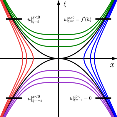
Figure 3: Level sets of $A_{3}$ singularity $H=\xi^{2}-x^{4}$. The four Lagrangian sections $\xi=\pm\varepsilon$, $x\lessgtr 0$ are shown in black. The four parts of the fibration, corresponding to the four functions $v_{i},$ are shown in colour.

Integrating $g(x,\xi)$ along the Hamiltonian flow of

$$\dot{x}=H_{\xi},\quad\dot{\xi}=-H_{x}$$

between these Lagrangian sections (i.e. along the characteristics of the linear PDE $\{H,u\}=g(x,\xi)$), produces 4 functions $v_{i}$ given explicitly as follows:

$$v_{1}(\xi,h)\equiv\tilde{u}(\xi,h)=\int_{-\varepsilon}^{\xi}\frac{g((t^{2}-h)^{\frac{1}{k}},t)}{-k(t^{2}-h)^{\frac{k-1}{k}}}\operatorname{d}\!{t},\quad v_{3}(\xi,h)=\int_{\varepsilon}^{\xi}\frac{g(-(t^{2}-h)^{\frac{1}{k}},t)}{k(t^{2}-h)^{\frac{k-1}{k}}}\operatorname{d}\!{t}$$ (65)

and

$$v_{2}(x,h)=\int_{(\varepsilon^{2}-h)^{1/k}}^{x}\frac{g(s,\sqrt{h+s^{k}})}{2\sqrt{h+s^{k}}}\operatorname{d}\!{s},\quad v_{4}(x,h)=\int_{-(\varepsilon^{2}-h)^{1/k}}^{x}\frac{g(s,-\sqrt{h+s^{k}})}{-2\sqrt{h+s^{k}}}\operatorname{d}\!{s}.$$ (66)

The global solution $u$ is now defined by the following rule:

• If $(x,\xi)$ is such that $x\geqslant 0$ and $H(x,\xi)\leqslant 0$, then $u(x,\xi)=\tilde{u}(\xi,H)=v_{1}(\xi,H)$ as above;

• If $(x,\xi)$ is such that $\xi\geqslant 0$ and $H(x,\xi)\geqslant 0$, we set $u(x,\xi)=h_{1}(H)+v_{2}(x,H),$ where $h_{1}(H)$ is any $C^{\infty}$-smooth function that coincides with $v_{1}(\varepsilon,H)\equiv f^{\prime}(H)$ on the Lagrangian section $\xi=\varepsilon,x>0$;

• Next, if $(x,\xi)$ is such that $x\leqslant 0$ and $H(x,\xi)\leqslant 0$, we set $u(x,\xi)=h_{1}(H)+h_{2}(H)+v_{3}(\xi,H),$ where $h_{2}(H)$ is any $C^{\infty}$-smooth function that coincides with $v_{2}(-(\varepsilon^{2}-H)^{1/k},H)$ on the Lagrangian section $\xi=\varepsilon,x<0$;

• Finally, if $(x,\xi)$ is such that $\xi\leqslant 0$ and $H(x,\xi)\geqslant 0$, we set $u(x,\xi)=h_{1}(H)+h_{2}(H)+h_{3}(H)+v_{4}(x,H),$ where $h_{3}(H)$ is any $C^{\infty}$-smooth function that coincides with $v_{3}(-\varepsilon,H)$ on the Lagrangian section $\xi=-\varepsilon,x<0$.

Observe that by the construction, we thus have $h_{1}(H)\equiv f^{\prime}(H)$ when $H\leqslant 0$. Moreover,

$$h_{1}(0)+h_{2}(0)+h_{3}(0)+h_{4}(0)=0,\quad\mbox{where}\quad h_{4}(0)=v_{4}(\varepsilon^{2/k},0),$$

since in this case we integrate twice along each of the 4 branches of $\xi^{2}-x^{2\ell}=0,\,k=2\ell,$ with opposite orientations. This shows that $u=u(x,\xi)$ is a well-defined and continuous function in a neighbourhood of the origin. Proceeding exactly as in Step 3, one can show that the functions $v_{1}(\xi,H)$ and $v_{3}(\xi,H)$ and hence also $h_{3}(H)$ are $C^{\infty}$-smooth. Writing

$$v_{2}(x(h,\xi),h)=\int_{\varepsilon}^{\sqrt{h}}\frac{g((t^{2}-h)^{\frac{1}{k}},t)}{k(t^{2}-h)^{\frac{k-1}{k}}}\operatorname{d}\!{t}+\int_{\sqrt{h}}^{\xi}\frac{g((t^{2}-h)^{\frac{1}{k}},t)}{k(t^{2}-h)^{\frac{k-1}{k}}}\operatorname{d}\!{t},$$ (67)

we see that also $v_{2}(\xi,H)$ are hence $h_{2}(H)$ are $C^{\infty}$-smooth. Indeed, we have already shown that in the preliminary normal form (64), all of the coefficients $d_{i}=0$ when $[\frac{i+1}{k}]<[\frac{n+1}{k}]$, which shows that these functions are at least $[\frac{n+1}{k}]-1$ times continuously differentiable. But the exponent $n$ is arbitrary large, which shows that these functions are in fact $C^{\infty}$-smooth.

A similar argument shows the smoothness of $v_{4}(\xi,H)$. We therefore get that $u$, being a sum of $v_{i}$ and $h_{j}$ on the closures of each connected component of $H^{-1}([-h_{0},h_{0}])\setminus H^{-1}(0)$, is $C^{\infty}$-smooth on each of these individual closures. Moreover, the vanishing of the coefficients $d_{i}=0$ in (64) implies that the corresponding derivatives match on $H^{-1}(0).$ It follows that $u$ is $C^{\infty}$-smooth. ∎

References

- [1] N. Abel. Auflösung einer mechanischen aufgabe. Journal für die reine und angewandte Mathematik, 1:153–157, 1826.
- [2] J. Alonso, H. Dullin, and S. Hohloch. Symplectic classification of coupled angular momenta. Nonlinearity, 33(1):417, 2019.
- [3] A. Bolsinov and A. Fomenko. Integrable Hamiltonian Systems: Geometry, Topology, Classification. CRC Press, 2004.
- [4] A. Bolsinov, L. Guglielmi, and E. Kudryavtseva. Symplectic invariants for parabolic orbits and cusp singularities of integrable systems. Phi. Trans. R. Soc. A., 376:20170424, 2018.
- [5] A. Bolsinov and A. Izosimov. Smooth invariants of focus-focus singularities and obstructions to product decomposition. Journal of Symplectic Geometry, 17(6):1613–1648, 2019.
- [6] A. Bolsinov, V. Matveev, E. Miranda, and S. Tabachnikov. Open problems, questions and challenges in finite-dimensional integrable systems. Phi. Trans. R. Soc. A., 376:20170430, 2018.
- [7] Y. Colin de Verdière. Singular Lagrangian manifolds and semiclassical analysis. Duke Math. J., 116(2):263–298, 2003.
- [8] Y. Colin de Verdière. A semi-classical inverse problem II: reconstruction of the potential. In Geometric aspects of analysis and mechanics, volume 292 of Progr. Math., pages 97–119. Birkhäuser/Springer, New York, 2011.
- [9] Y. Colin de Verdiere and J. Vey. Le lemme de Morse isochore. Topology, 18(4):283 – 293, 1979.
- [10] R. H. Cushman and L. M. Bates. Global aspects of classical integrable systems. Birkhäuser, 2 edition, 2015.
- [11] T. Delzant. Hamiltoniens périodiques et images convexes de l’application moment. Bulletin de la Société mathématique de France, 116(3):315–339, 1988.
- [12] G. Dhont and B. Zhilinskií. Classical and quantum fold catastrophe in the presence of axial symmetry. Phys. Rev. A, 78:052117, 2008.
- [13] J. J. Duistermaat. On global action-angle coordinates. Communications on Pure and Applied Mathematics, 33(6):687–706, 1980.
- [14] K. Efstathiou and A. Giacobbe. The topology associated with cusp singular points. Nonlinearity, 25(12):3409–3422, 2012.
- [15] L. H. Eliasson. Hamiltonian systems with Poisson commuting integrals. PhD thesis, Stockholm University, 1984.
- [16] L. H. Eliasson. Normal forms for Hamiltonian systems with Poisson commuting integrals — elliptic case. Commentarii Mathematici Helvetici, 65:4–35, 1990.
- [17] J.-P. Françoise. Modèle local simultané d’une fonction et d’une forme de volume. Journées singulières de Dijon, Astérisque, 59–60:119–130, 1978.
- [18] J.-P. Françoise. Relative cohomology and volume forms. Banach Center Publications, 20(1):207–222, 1988.
- [19] J.-P. Françoise. Intégrales de périodes en géométries symplectique et isochore. Géométrie Symplectique et Mécanique (La Grande Motte, 1988). Volume 1416 of Lecture notes in Mathematics. Springer Berlin Heidelberg, 1990.
- [20] M. D. Garay. Stable moment mappings and singular Lagrangian foliations. Quart. J. Math, 56:357–366, 2005.
- [21] L. Guglielmi. Symplectic invariants of integrable Hamiltonian systems with singularities. PhD thesis, SISSA, 2018.
- [22] S. Hohloch and J. Palmer. Extending compact Hamiltonian -spaces to integrable systems with mild degeneracies in dimension four. arXiv:2105.00523, 2021.
- [23] A. Izosimov. Classification of almost toric singularities of Lagrangian foliations. Sbornik: Mathematics, 202(7):1021–1042, 2011.
- [24] E. Kudryavtseva. Hidden toric symmetry and structural stability of singularities in integrable systems. Europ. J. Math., 8:1487–1549, 2022.
- [25] E. Kudryavtseva and N. Martynchuk. symplectic invariants of parabolic orbits and flaps in integrable Hamiltonian systems. arXiv:2110.13758, 2021.
- [26] E. Kudryavtseva and N. Martynchuk. Existence of a smooth Hamiltonian circle action near parabolic orbits and cuspidal tori. Regular and Chaotic Dynamics, 26(6):732–741, 2021.
- [27] E. Kudryavtseva and A. Oshemkov. Structurally stable non-degenerate singularities of integrable systems. Russian Journal of Mathematical Physics, 29:58–75, 2022.
- [28] Y. Le Floch and Á. Pelayo. Symplectic geometry and spectral properties of classical and quantum coupled angular momenta. J. Nonlinear Sci., 29:655–708, 2019.
- [29] O. V. Lukina, F. Takens, and H. W. Broer. Global properties of integrable Hamiltonian systems. Regular and Chaotic Dynamics, 13(6):602–644, 2008.
- [30] E. Miranda and N. T. Zung. Equivariant normal form for nondegenerate singular orbits of integrable Hamiltonian systems. Annales Scientifiques de l’École Normale Supérieure, 37(6):819 – 839, 2004.
- [31] F. W. J. Olver, D. W. Lozier, R. F. Boisvert, and C. W. Clark, editors. NIST handbook of mathematical functions. U.S. Department of Commerce, National Institute of Standards and Technology, Washington, DC; Cambridge University Press, Cambridge, 2010. With 1 CD-ROM (Windows, Macintosh and UNIX).
- [32] Á. Pelayo and S. Vũ Ngọc. Semitoric integrable systems on symplectic 4-manifolds. Invent. math., 177:571–597, 2009.
- [33] Á. Pelayo and S. Vũ Ngọc. Constructing integrable systems of semitoric type. Acta Mathematica, 206(1):93–125, 2011.
- [34] S. Vũ Ngọc. Systèmes intègrables semi-classiques: du local au global. Panoramas et Synthèses SMF, 2006.
- [35] S. Vũ Ngọc. Symplectic inverse spectral theory for pseudodifferential operators. In Geometric aspects of analysis and mechanics, volume 292 of Progr. Math., pages 353–372. Birkhäuser/Springer, New York, 2011.
- [36] S. Vũ Ngọc and C. Wacheux. Smooth normal forms for integrable Hamiltonian systems near a focus-focus singularity. Acta Math Vietnam., 38(2):107–122, 2013.
- [37] J. C. van der Meer. The Hamiltonian Hopf Bifurcation. Springer, Springer-Verlag Berlin Heidelberg, 1985.
- [38] S. Vũ Ngọc. On semi-global invariants for focus-focus singularities. Topology, 42:365–380, 2003.
- [39] H. Waalkens, H. R. Dullin, and P. H. Richter. The problem of two fixed centers: bifurcations, actions, monodromy. Physica D: Nonlinear Phenomena, 196(3-4):265–310, 2004.
- [40] N. T. Zung. Symplectic topology of integrable Hamiltonian systems, I: Arnold-Liouville with singularities. Compositio Mathematica, 101(2):179–215, 1996.