Modeling the induced voltage of a disk magnet in free fall
Abstract
We drop a circular disk magnet through a thin coil of wire, record the induced voltage, and compare the results to an analytic model based on the dipole approximation and Faraday’s law, which predicts that the difference between the voltage peak magnitudes corresponding to the entry and exit of the magnet should be in proportion to , where is the initial height of the magnet above the center of the coil. Agreement between the model and experimental data are excellent. This easily-reproduced experiment provides an opportunity for students at a range of levels to quantitatively explore the effects of magnetic induction.
I Introduction
Faraday’s law of electromagnetic induction is fundamental to any introductory physics sequence. While it is straightforward to demonstrate qualitatively, providing students with a quantitative experiment is more challenging. A common approach is to drop a magnet through a conducting loop and measure consequences of that relative motion. These experiments tend to fall into two basic categories: (i) inducing resistive magnetic forces via eddy currents, [1, 2, 3, 4, 5] and (ii) inducing a voltage signal that is visualized in real time using computer acquisition software. [6, 7, 8, 9, 10] In this paper, we follow the second group and describe an experiment where students drop a circular disk magnet through an induction coil and relate the resulting peak voltage values to the drop height of the magnet. Such an approach presents a good mix of intuition gained from introductory mechanics and electromagnetic phenomena. The recent paper of Gadre et al. describes an experiment similar to that which we describe here, but our analysis is more thorough and explicitly compares experimental results to theoretical predictions. [10] While some of the details provided here are outside the scope of an introductory-level course, they would be accessible to upper-level students, and are critical to the discussion contained herein.
II Free-falling magnet
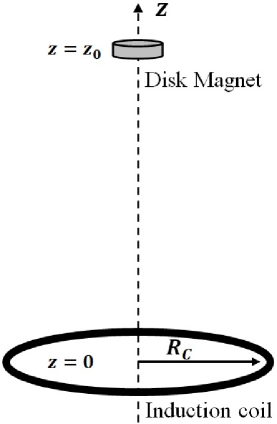
In this section we provide an analytic model for the induced voltage signal produced by a disk magnet falling freely through an open coil of radius and negligible thickness. As shown in Fig. 1, the starting height of the magnet is defined as the distance from the mid-point of the coil to the mid-point of the magnet, which is assumed to fall freely through the center of the coil along the -axis. We ignore air drag as well as any resistive magnetic forces that act on the magnet from the coil.
II.1 Modeling the disk magnet
We assume that a circular disk magnet can be modeled as an ideal -turn circular loop of current , with dimensions equal to that of the magnet, save for the thickness, which we assume to be negligible. As the magnet falls along the -axis through the induction coil, only the -component of the magnetic field will contribute to the flux, and thus to the induced voltage. Therefore, we only need to concern ourselves with the -component of the magnetic field, which can be found using the Biot-Savart law and the standard dipole approximation: [11]
| (1) |
Here, is the radius of the magnet, is the cylindrical coordinate of the field point, and we have set , where is an empirical constant to be determined. The total magnetic flux (linkage) of such a field through the open area of an induction coil with radius and number of turns is found via direct integration to be:
| (2) |
A full derivation of Eqs. (1) and Eq. (2) appears in the Supplementary Material. [12]
II.2 Modeling the Voltage Signal
For a magnet that is moving, and so Eq. (2) becomes a function of time where the flux increases as the magnet approaches the coil, reaches a maximum when it is at the center of the coil, and then decreases as it exits the coil. The resulting voltage signal in the coil is found from Faraday’s law of induction and the chain rule to be:
| (3) |
where is the speed of the moving magnet. When the speed is constant, Eq. (3) is an anti-symmetric function: the two voltage peaks occur at and ( at the center of the coil), and the peaks are equal in value but opposite in polarity. This was extensively verified in Kingman, et. al. [7]
For an accelerating magnet, Eq. (3) is no longer exactly anti-symmetric. Since the speed of the magnet is higher as it exits the coil than when it enters, we should expect the later peak voltage to be larger than the earlier one . Further, the voltage peaks do not occur exactly at ; however, the shifts away from these points are small enough to ignore (see Appendix A).
Since measuring the instantaneous speed of an accelerating (free falling) magnet is difficult, we instead seek a relationship between the initial height of the magnet and the measured peak voltages of the signal. For a magnet in free fall, its speed at any position is related to the drop height through kinematics: . Inserting this into Eq. (3) and assuming the peak voltages occur at the specific positions , we find the peak voltage values to be:
| (4) |
If we further assume that the peak positions occur approximately at and and let the drop height be much larger than these positions (i.e. ), we can expand the square root and find:
| (5) | ||||
| (6) |
Here, is the first (earlier) peak voltage and is the second (later) peak voltage. We express the results as magnitudes since the polarity depends on the experimental set up. We note that the difference between the magnitudes of the two peaks asymptotically approaches zero with increasing drop height:
| (7) |
While upper-level E&M students should be capable of applying the binomial expansion, a more qualitative argument for the -dependence can be made for introductory students by noting that the difference in the peak voltage values is proportional to the difference in the corresponding speed values, i.e. . Here, , where is the time between the peaks. If the drop height is sufficiently large, then will be much smaller than the total drop time and so the magnet’s change in speed will be minimal during this interval. Approximating the speed as an average value during this time yields , where is the vertical distance traveled during and , which is the magnet’s speed at the center of the coil. Thus, we arrive at , which is straightforward to verify experimentally.
III Experiment
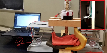
A disk magnet of radius cm and thickness cm was taped to a plastic ruler to facilitate consistent dropping through a -turn coil of copper wire wrapped around a piece of ABS plastic piping. The coil, of average radius cm and thickness cm, was set on two blocks of wood and elevated by two jack stands; foam padding was set beneath the coil to protect the magnet as it fell, and a meter stick was stationed inside the coil to measure the drop height; see Fig. 2. While it might not be obvious that the dipole approximation should apply here given the relative dimensions of the magnet and the coil, we will see below that it does yield a very good fit with the experimental data.
To determine the -value of the disk magnet, a FW Bell model 4048 Gauss/Tesla meter ( tolerance) was used to measure the magnetic field along the main axis from 4.0 cm to 10.5 cm in 0.5 cm intervals. We plotted vs. and found Tm from the slope of the linear fit. [12] This corresponds to a magnetic dipole moment of Am2.
III.1 Data Acquisition
The voltage measurements were made with a Pasco 750 Computer Interface in conjunction with Pasco Capstone software. As the magnet fell through the main axis of the coil, the software displayed the induced voltage signal as a function of time; a 2,000 Hz sampling rate was used for every trial. The starting height of the magnet was varied from 1.0 cm to 5.0 cm in 1.0 cm intervals, and then 5.0 cm to 45 cm in 2.5 cm intervals. All values are measured from the center of the coil . For each starting height, the magnet was dropped five times and the two peak voltages were recorded for every trial; all results are thus presented as an average (data point) and an uncertainty (error bars).
III.2 Results
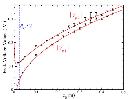
In Fig. 3 we plot the experimental peak voltage values against the drop height, along with the theoretical predictions given by Eq. (5) and Eq. (6). The uncertainties are given by the sample standard deviation of the mean of the measurements, while the the theoretical curves were obtained directly from Eqs. (5) and (6), along with the experimental parameters defined earlier. We find very good agreement between the experimental data and the theoretical models for drop heights greater than 2.4 cm, which was an assumed condition in the derivation of Eqs. (5) and (6). We mark the position explicitly in Fig. 3 and Fig. 4, and note that the model begins to break down for drop heights less than this value.
The upper limit of the data set was mainly a practical one: consistently dropping the magnet through the center of the induction coil became too difficult for drop heights larger than 45 cm. While drag effects could also begin to manifest at larger drop heights, we show later that these effects are minimal for the magnet used in this experiment.
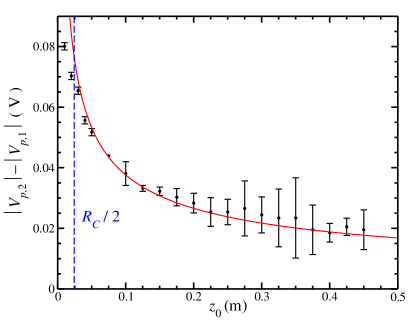
As mentioned earlier, the -dependence is key to accurately modeling the peak voltage magnitudes. We demonstrate this explicitly in Fig. 4 by plotting the difference between the peak voltages against the drop height. The uncertainties are found via propagation of the error values given in Fig. 3. We again find the theoretical curve by applying the relevant experimental parameters directly to Eq. (7), and find very good agreement for all drop heights larger than 2.4 cm.
Finally, if we define Eq. (3) explicitly as a function of time by letting and , we arrive at the following expression which can be numerically evaluated:
| (8) |
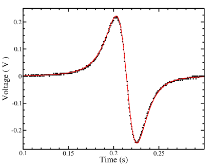
In Fig. 5 we match the complete theoretical line shape as predicted by Eq. (8) to the induced voltage signal for a representative sample run ( cm); the agreement between the experimental signal and the theoretical model is essentially perfect. This further validates the analytical approach taken in Section II.
III.3 Error and Limitations
For the experiment described here, the largest source of experimental error comes from dropping the magnet by hand through the center of the induction coil from the same height for any five repeated trials. Anecdotally, it was observed that if the magnet drifted away from the symmetry axis as it fell, the voltage peaks were affected by this motion. The data indicates that this was more of an issue at larger drop heights, where the average peak voltage values tend to skew larger than the theoretical line shapes, in particular for the later peak. While numerical modeling seems to suggest that a falling magnet with non-zero horizontal motion can result in a larger flux change (and thus larger voltage peaks), we cannot conclusively verify this yet. Overall, however, these effects seem to be random, and they are small: differences between the data points and the predicted curves are on the order of millivolts, which begins to approach the tolerance of the instrumentation.
For larger drop heights, it is also reasonable to suspect that air drag would begin to affect the magnet’s speed and thus affect the voltage measurements. We modeled a quadratic drag force on the square 2.30 cm 2.30 cm cross section of masking tape holding the magnet to the ruler (total mass of 0.02 kg), and found that air drag accounted for a reduction of only 0.6% of the speed at the largest drop height used in this experiment.
Similarly, resistive drag effects due to the induced currents in the coil were also minimal. Since air resistance is not a significant factor, the magnet’s kinetic energy at the center of the coil should be equal to its potential energy at release , which is 88 mJ for the largest drop height used in this experiment. The energy lost due to inducing a current in the coil is found by integrating the electric power over time:
| (9) |
where is defined in Eq. (8) and is the resistance of the coil, measured to be 21.7 . This calculation yields an energy loss of 0.123 mJ for the largest drop height, roughly of the initial energy. Repeating for the smallest drop height yielded an initial energy value of 1.96 mJ and an energy loss of 0.0188 mJ, or about .
The theoretical model hinges on two main assumptions. One is that the drop height of the magnet is much larger than half the coil radius. This allows us to define the locations of the voltage extrema at as well as to employ the binomial expansion on the speed term in the peak voltage definitions. This assumption also coincides with the range of validity for the dipole approximation.
The second assumption is that both the magnet and the induction coil be treated as “thin rings” of negligible thickness. For a cylindrical object, this approximation is gauged by the ratio of the cylinder’s length to its diameter ; as long as this ratio is “small enough,” the approximation is valid. Determining exactly where this approximation breaks down depends on the details of the individual experiment, but for the objects used here, the magnet had an ratio of about , while the induction coil had a ratio of about . Based on the results of our experiment, we conclude that these ratios are indeed “small enough” for the models to be considered valid. Separate numerical modeling (not shown) indicates that the thin ring model for the induction coil begins to noticeably separate from the solenoid model around which would correspond to the edges of the coil being located at the assumed peak voltage positions . While this should not necessarily be considered the point at which the model breaks down, it could serve as a rough upper limit when designing the experiment.
IV Conclusion
In this paper, we have developed an analytic model of the induced voltage signal produced by a disk magnet falling freely through a thin induction coil. The initial motivation for this work was to develop a quantitative experiment to test Faraday’s law; however, we were pleasantly surprised at the robust opportunities for engagement of students at various course levels that this investigation provides. All of the measurements are easily obtained in an introductory setting, requiring materials and equipment either generally available or easy to obtain.
While a similar but slightly more rigorous derivation of the peak voltage values can be done in the time coordinate, the argument presented here in the -coordinate allows students to make an intuitive connection between introductory kinematics and the observed voltage signals. Students can be led through a series of questions and/or asked to make their own speculations about what they expect to see based on their knowledge of free fall. At the introductory level, students could then simply measure the drop height of the magnet , the two resulting voltage peak values , , and test their predictions. It would also be straightforward at that point to verify the -dependence of (as in Fig. 4). Depending on the expectation of the level of rigor for the experiment, students could also measure the experimental parameters required to plot the theoretical curve for direct comparison to the data set.
In an upper-level course, students could be expected to replicate some or all of the derivations contained in this paper [12], have a stronger understanding of the model, and be able to explore the consequences of varying different parameters on the resulting voltage signal. For example, magnets of different radii or dipole moments could be used, along with different induction coils of varying radii or number of turns. For comparison to the experimental voltage signals, theoretical line shapes are easily produced using any graphing software or numerical coding platforms. While the application of the dipole approximation makes the full model accessible to upper-level students, it is also conceivable that it could be eschewed in favor of a complete elliptic integral approach that could be investigated as part of an advanced project; this could be done while experimenting with an induction coil that is similar in size to the magnet.
Finally, the work included here could be extended to examine a disk magnet moving through a solenoid induction coil rather than a thin-ring coil, or a bar magnet moving through various coil geometries. It could also be interesting to evaluate the resulting voltage signals of a disk magnet moving with varied accelerations as controlled via an Atwood’s machine.
Appendix A Approximating the Peak Voltage Positions
Beginning with Eq. (3) and applying the free-fall condition for , we arrive at the following general expression for the voltage signal as a function of position :
| (10) |
The voltage peaks for this signal occur at the peak position (assuming at the center of the coil), where the derivative of Eq. (10) is equal to zero. Taking the derivative with respect to , setting equal to zero, and simplifying yields:
| (11) |
While these values can be solved for numerically, the results are not particularly instructive. Instead, we can reasonably approximate values for by assuming that the drop height is much larger than . Factoring out a gives
| (12) |
Ignoring the cubic term, we can solve the remaining quadratic for :
| (13) |
which we can further simplify by applying the condition that :
| (14) |
Thus, if the drop height is (much) larger than half the radius of the induction coil, the voltage peaks will occur approximately at , which is where they peak in the constant-speed case.
Acknowledgements.
The author gratefully acknowledges Joseph Gallant for carefully proof-reading early versions of this manuscript, Karl Martini and Sam Emery for discussions of uncertainty analysis, and the reviewers for their thoughtful comments, helpful suggestions, and overall insight.The author has no conflicts to disclose.
References
- Derby and Olbert [2010] N. Derby and S. Olbert, Cylindrical magnets and ideal solenoids, American Journal of Physics 78, 229 (2010), https://doi.org/10.1119/1.3256157 .
- Hahn et al. [1998] K. D. Hahn, E. M. Johnson, A. Brokken, and S. Baldwin, Eddy current damping of a magnet moving through a pipe, American Journal of Physics 66, 1066 (1998), https://doi.org/10.1119/1.19060 .
- Levin et al. [2006] Y. Levin, F. L. da Silveira, and F. B. Rizzato, Electromagnetic braking: A simple quantitative model, American Journal of Physics 74, 815 (2006), https://doi.org/10.1119/1.2203645 .
- Roy et al. [2007] M. K. Roy, M. K. Harbola, and H. C. Verma, Demonstration of lenz’s law: Analysis of a magnet falling through a conducting tube, American Journal of Physics 75, 728 (2007), https://doi.org/10.1119/1.2744047 .
- Irvine et al. [2014] B. Irvine, M. Kemnetz, A. Gangopadhyaya, and T. Ruubel, Magnet traveling through a conducting pipe: A variation on the analytical approach, American Journal of Physics 82, 273 (2014), https://doi.org/10.1119/1.4864278 .
- Nicklin [1986] R. C. Nicklin, Faraday’s law—quantitative experiments, American Journal of Physics 54, 422 (1986), https://doi.org/10.1119/1.14606 .
- Kingman et al. [2002] R. Kingman, S. Rowland, and S. Popescu, An experimental observation of faraday’s law of induction, American Journal of Physics 70, 595 (2002).
- Amrani and Paradis [2005] D. Amrani and P. Paradis, Electromotive force: Faraday’s law of induction gets free-falling magnet treatment, Physics Education 40, 313 (2005).
- Reeder et al. [2019] S. Reeder, K. Wilkie, T. Kelly, and J. Bouillard, Insights into the falling magnet experiment, Physics Education 54, 055017 (2019).
- Gadre et al. [2023] D. V. Gadre, H. Sharma, S. D. Gadre, and S. Srivastava, Science on a stick: An experimental and demonstration platform for learning several physical principles, American Journal of Physics 91, 116 (2023).
- Jackson [1999] J. D. Jackson, Classical Electrodynamics, Third Edition (John Wiley & Sons, Hoboken, NJ, 1999).
- [12] Supplemental material can be found at [URL to be inserted by AIPP]