Uncertainty Quantification of Mass Models Using Ensemble Bayesian Model Averaging

Abstract

Developments in the description of the masses of atomic nuclei have led to various nuclear mass models that provide predictions for masses across the whole chart of nuclides. These mass models play an important role in understanding the synthesis of heavy elements in the rapid neutron capture ($r$-) process. However, it is still a challenging task to estimate the size of uncertainty associated with the predictions of each mass model. In this work, a method to quantify the mass uncertainty using ensemble Bayesian model averaging (EBMA) is introduced. This Bayesian method provides a natural way to perform model averaging, selection, calibration, and uncertainty quantification, by combining the mass models as a mixture of normal distributions, whose parameters are optimized against the experimental data, employing the Markov chain Monte Carlo (MCMC) method using the No-U-Turn sampler (NUTS). The average size of our best uncertainty estimates of neutron separation energies based on the AME2003 data is 0.48 MeV and covers 95 % of new data in the AME2020. The uncertainty estimates can also be used to detect outliers with respect to the trend of experimental data and theoretical predictions.

I Introduction

Since the first introduction of the nuclear liquid drop model, the theoretical description of nuclear masses has seen great progress, which gave rise to many related but different approaches. It is now possible to describe the ground state properties of nuclei across the chart of nuclei with theories of different scales: Macroscopic-microscopic theories such as the Finite-Range Droplet Model (FRDM) [1, 2], Weizsäcker-Skyrme (WS) models [3, 4, 5, 6], microscopically inspired Duflo-Zucker models [7], and more microscopic theories such as nuclear density functional theory (DFT) with different interactions or energy density functionals (EDFs) [8, 9, 10].

These global mass models play an important role in understanding the origin of heavy elements in the Universe via the rapid neutron capture ($r$-) process [11, 12, 13]. This is because the nuclear masses determine the $Q$-value (energy release) of nuclear reactions and decays, which also affect their rates (e.g., $\beta$-decay rates $\propto Q^{3\text{--}7}$ [14, 15]). However, the masses of the vast majority of neutron-rich nuclei relevant to the $r$-process have yet to be experimentally studied. Therefore, the mass models used in nucleosynthesis studies have a significant impact on the resulting abundance patterns and kilonova lightcurves [16, 17].

One of the challenges in understanding the impact of mass models on nucleosynthesis is that, in general, uncertainty estimates associated with the theoretical masses are not available. Although there has been an effort to quantify an uncertainty in microscopic theories [18, 19], the mass models that are commonly used in nucleosynthesis studies, especially macroscopic-microscopic and phenomenological models, do not come with a quantified prediction uncertainty. The root mean square (RMS) error of each mass model can be calculated with respect to the observations, but it most likely underestimates the uncertainty where there is no data (see Figure 1).

Furthermore, the possibility of quantifying the uncertainty by combining multiple mass models and observations has been largely unexplored. This poses a challenge in quantifying the uncertainty in the $r$-process nucleosynthesis that arises from uncertain nuclear masses.

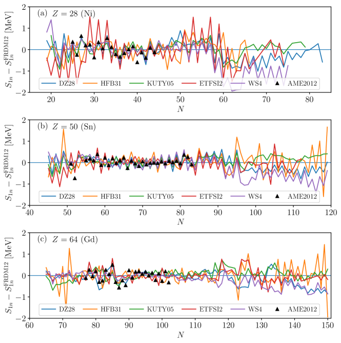
Figure 1: Comparison of one-neutron separation energies ($S_{1n}$) predicted by each mass model used in this study and the experimental masses from the AME2020 [20], relative to the predictions of the FRDM2012 for (a) $Z=28$ (Ni), (b) $Z=50$ (Sn), and (c) $Z=64$ (Gd) isotopes. The mass models and references are listed in Section II.3

.

As the next-generation radioactive isotope beam facilities allow us to gain access to more neutron-rich isotopes, it will become possible to test the performances of the mass models in the extremely neutron-rich regions of the chart of nuclides. In experimental studies of nuclear masses, usually only the new experimental results are compared with the theoretical predictions. It is often done by calculating the RMS error, but this does not fully combine all the available experimental data. Therefore, a statistical method to test the predictions of various theoretical models and evaluate the impact of new measurements on the uncertainty of extrapolated masses would be an improvement over the current situation.

In this work, we will apply a method called ensemble Bayesian model averaging (EBMA) introduced by Ref. [21] to combine available experimental data and multiple theoretical mass models, as well as to quantify the mass uncertainty. This method models an ensemble of theoretical mass models as a mixture of normal distributions, whose parameters are estimated based on the observations. The EBMA combines model calibration, selection, averaging, and uncertainty quantification in a single framework. The resulting probabilistic model is highly interpretable. This Bayesian method is quite general and can be readily applied to other nuclear physics observables.

Recently, data-driven modeling of nuclear masses using machine learning techniques has gained popularity [22, 23, 24, 25, 26, 27, 28, 29, 30]. Probabilistic models have especially achieved high accuracy while providing an estimate for the uncertainty. Although there have been attempts to construct physically interpretable models [29], it is generally challenging to gain insight into the underlying physics from machine learning models. Nevertheless, the advantages of machine learning models are that they can be created rapidly and often achieve similar performance to state-of-the-art theoretical models. Although they may not be able to predict new or unknown physics, they can combine physics that they learn in potentially novel ways that are difficult to produce through standard modeling.

The purpose of this study is not to create another mass model or to improve existing ones with machine learning. Rather, the aim is to investigate how well an ensemble of theoretical models can reproduce experimental data and quantify the performance of each model in the ensemble. This quantifies the uncertainty in extrapolating the experimental data. Our approach should be considered as a method for model averaging, selection, calibration, and uncertainty quantification, using only existing theoretical models.

This paper is divided into the following sections: in Sec. II, we discuss the details of the EBMA method and the numerical experiment where we construct EBMA models; in Sec. III, we discuss the results of the different approaches for constructing EBMA models and the details of the quantified uncertainties for one neutron separation energies ($S_{1n}$); finally, we summarize the work presented in the paper and describe possible applications in Sec. IV.

II Method

II.1 Bayesian model averaging

Bayesian model averaging (BMA) is applicable when more than one statistical model that describes the data reasonably well is available, and one wishes to account for the uncertainty in the analysis arising from conditioning on a single model. BMA computes a weighted average of the probability density functions (PDFs), weighted by the posterior probability of the “correctness” of each model given the training data. Following the description in Refs. [31, 21], the posterior distribution of the observable of interest $\Delta$, defined by BMA, is

$$p(\Delta\mid D)=\sum_{k=1}^{K}\;p(\Delta\mid M_{k},D)\;p(M_{k}\mid D),$$ (1)

where $p(\Delta\mid M_{k},D)$ is the posterior PDF of the observable of interest based on a single statistical model $M_{k}$, and $p(M_{k}\mid D)$ is the corresponding posterior model probability, which represents how well the model $M_{k}$ fits the data $D$. The posterior model probabilities can be considered as weights, since their sum is equal to 1.

II.2 Ensemble Bayesian model averaging

One of the limitations in the applicability of the BMA method is that the participating models themselves must be probabilistic. In nuclear physics, most models are not probabilistic. Therefore, we need to extend the BMA framework to handle such models. Raftery et al. [21] introduced the ensemble Bayesian model averaging (EBMA) method, which computes the weighted average of an ensemble of bias-corrected models, as a finite mixture of normal distributions. In the EBMA framework, the predictive model is

$$p(\Delta\mid m_{1},\ldots,m_{k})=\sum_{k=1}^{K}\;w_{k}\;g_{k}(\Delta\mid m_{k}),$$ (2)

where $w_{k}$ is the weight of the model $m_{k}$, whose posterior represents the probability of the model $k$ being the best one, based on the observed data $D$. Since the size of the weight depends on the relative performance of the model, even if the ensemble includes an extremely inaccurate model, its effect on the predictive distributions of EBMA is quite small, since an extremely small weight would be assigned to the model. $g_{k}(\Delta\mid m_{k})$ is a normal PDF with its mean defined by the bias-corrected model predictions and standard deviation $\sigma_{k}$:

$$g_{k}(\Delta\mid m_{k})=N(\Delta\mid a_{k}+b_{k}m_{k},\sigma_{k}^{2}),$$ (3)

where $a_{k}$ and $b_{k}$ are the bias-correction coefficients, which are discussed in more detail in the following section. In the original EBMA by Raftery et al. [21], a constant standard deviation was used across all the models in the ensemble; however, we take it as model dependent (denoted by the subscript $k$), which is a more natural way to construct a mixture model.

II.2.1 Bias correction

In constructing EBMA models, although not strictly necessary, Ref. [21] linearly corrects the bias of the prediction of each model, as shown in Equation 3. Since most mass models are already fitted to the experimental data, the values of the bias-correction coefficients are expected to be $a_{k}\sim 0$ and $b_{k}\sim 1$, where they correct the offset and slope of the model, respectively. The original prediction of the model corresponds to $a_{k}=0$ and $b_{k}=1$.

Ref. [21] suggests that $a_{k}$ and $b_{k}$ for each $k=1,\ldots,K$ are determined by linear regression. Another way to determine these parameters $a_{k}$ and $b_{k}$ is by Bayesian linear regression and taking the maximum a posteriori (MAP) values, which is a slightly more probabilistic treatment. In our case, the two approaches yield virtually identical values. The coefficients determined for each mass model using the entire AME2020 data are shown in Table 1, for example. For some mass models, the values of $a_{k}$ are significantly different from 0. This is most likely because different sets of experimental data were used in the original construction of the mass models.

Table 1: Bias-correction coefficients determined for different mass models from the MAP values of Bayesian linear regression (labeled as “BLR MAP”) and usual linear regression (labeled as “LR”), respectively, using all of the available AME2020 [20] one-neutron separation energy ($S_{1n}$) data. $a_{k}$ and $b_{k}$ are the coefficients for offset (intercept) and slope, respectively, for mass model $k$. The values are rounded to two digits.

	$a_{k}$		$b_{k}$
Mass model	BLR MAP	LR	BLR MAP	LR
WS4 [6]	-0.02	-0.02	1.00	1.00
DZ29 [7]	-0.12	-0.12	1.01	1.01
FRDM12 [2]	0.05	0.05	0.99	0.99
KUTY05 [32]	0.43	0.43	0.94	0.94
ETFSI2 [33]	0.76	0.76	0.90	0.90
HFB31 [10]	0.21	0.21	0.97	0.97

II.2.2 Bayesian inference

The parameters of interest in our statistical inference are the weights $w_{k}\;(k=1,\ldots,K)$ and the standard deviations of the normal distributions that correspond to each of the theoretical mass models in the ensemble. Therefore, prior distributions for the parameters must be specified. In general, we try to choose the prior distributions to be as weakly informative as possible. For the weights, since they have to sum up to one $\left(\sum_{k=1}^{K}w_{k}=1\right)$, we model the parameters with a Dirichlet distribution of order $K$, which meets this requirement. Therefore, the prior for the weights is

$$p (w_{1},w_{2},\;\ldots,\;w_{k})$$

$$=\mathrm{Dirichlet}(w_{1},w_{2},\;\ldots,\;w_{k}\mid\alpha_{1},\alpha_{2},\;\ldots,\;\alpha_{k})$$

$$=\frac{\Gamma\left(\sum_{k=1}^{K}\alpha_{k}\right)}{\prod_{k=1}^{K}\Gamma(\alpha_{k})}\prod_{k=1}^{K}w_{k}^{\alpha_{k}-1},$$ (4)

where $\alpha_{1},\alpha_{2},\;\ldots,\;\alpha_{k}$ are called the “concentration parameters”, and $\Gamma(\cdot)$ is the gamma function $\left(\Gamma(z)\equiv\int_{0}^{\infty}t^{z-1}e^{-t}\mathrm{d}t\right)$. The concentration parameters of the Dirichlet distribution are set to 1 to ensure that the prior distributions are only weakly informative. The prior distributions for the standard deviations are chosen to be exponential distributions with the rate parameters equal to 1, which has been suggested to be one of the weaker priors [34].

The likelihood of the normal mixture model is defined as

$$L (w_{1},\;\ldots,\;w_{K},\;\sigma_{1}^{2},\;\ldots,\;\sigma_{K}^{2})$$

$$=\prod_{(N,Z)}\left(\sum_{k=1}^{K}w_{k}g_{k}(\Delta_{(N,Z)}\mid m_{k,(N,Z)})\right),$$ (5)

where the subscript $(N,Z)$ represents pairs of neutron number $n$ and proton number $p$ of the nuclei where observations exist. In practice, the logarithm of the likelihood (log-likelihood) is often used for computation to avoid numerical problems.

With the prior distributions and the likelihood function, it is now possible to formulate the posterior distributions for the parameters of the EBMA model.

$$p(\bm{w},\bm{\sigma^{2}}\mid D)\propto L(\bm{w},\bm{\sigma^{2}})\;p(\bm{w})\;p(\bm{\sigma^{2}}),$$ (6)

where $\bm{w}=w_{1},\ldots,w_{K}$, $\bm{\sigma^{2}}=\sigma_{1}^{2},\ldots,\sigma_{K}^{2}$, and $D$ denotes observational data. The prior distributions are denoted as $p(\bm{w})$ and $p(\bm{\sigma}^{2})$, respectively.

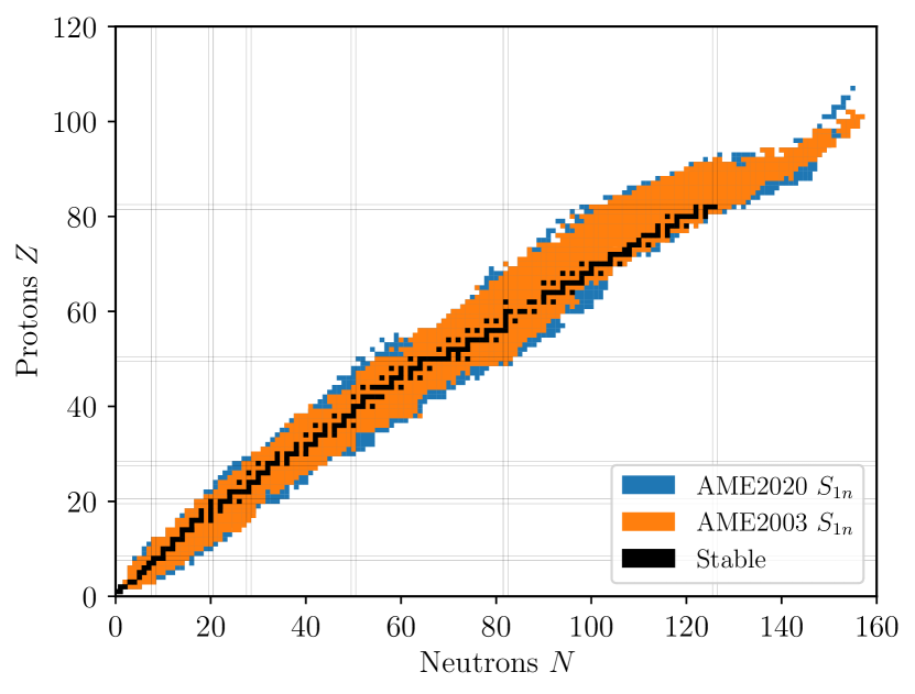
Figure 2: Comparison of the AME2003 data with the latest AME2020 data for one-neutron separation energies $S_{1n}$, illustrated on the chart of nuclides. The blue squares show the new $S_{1n}$ data in the AME2020 that did not exist in the AME2003. The $S_{1n}$ values listed in the AME2003 are shown in orange color, aside from the stable nuclides, shown in black.

II.2.3 Predictive variance

In EBMA models, the uncertainty of the quantity of interest is provided in the form of variance of the posterior predictive distribution. Based on Ref. [21] but reflecting the fact that our $\sigma_{k}$ depends on model $k$, the predictive variance can be written as

$$\mathrm{Var} (\Delta\mid m_{1},m_{2},\ldots,m_{K})$$

$$= \sum_{k=1}^{K}w_{k}\left((a_{k}+b_{k}m_{k})-\sum_{i=1}^{K}w_{i}(a_{i}+b_{i}m_{i})\right)^{2}$$

$$+\sum_{k=1}^{K}w_{k}\sigma_{k}^{2},$$ (7)

where the first term corresponds to the spread of predictions by the member mass models of the ensemble, and the second term corresponds to the expected deviation from the observations of each mass model, weighted by the posterior weights.

II.2.4 Differences to related works and discussion of models

It is worth discussing the key differences between our framework and related studies that use the BMA method, namely Refs.[24, 25, 35, 36, 37]. In their BMA framework, the uncertainty quantification of the considered mass models is performed by constructing Gaussian Process (GP) emulators, which learn the corrections to the mass models from the residuals with respect to the observed values. Therefore, the quality of the prediction and the corresponding uncertainty mainly depend on the performance of the GP emulator. The BMA weights are calculated either based on some criteria such as nuclei being bound or the performances of each mass model on the test data. One of the drawbacks of this method is that the derived weights are point estimates, and the resulting BMA uncertainty is a deterministic weighted average of the GP uncertainties. Furthermore, one has to be cautious when performing extrapolations using GPs, since an unconstrained GP converges to its mean with fixed uncertainty away from the data [38, 39].

On the other hand, the EBMA framework keeps the point predictions of the mass models in the ensemble. Instead, the weights and variances associated with each mass model are modeled probabilistically based on the experimental data. The probabilistic distributions are reflected onto the resulting predictive uncertainty through the Bayesian framework. In this framework, the predictions of each mass model that constitute the EBMA model are only linearly calibrated; therefore, the local trend of the predictions remains unchanged.

One of the shortcomings of the current method is that the inference of posterior weights is performed assuming that all observed data points are equally relevant. In the case of uncertainty quantification of mass models for neutron-rich nuclei, for example, one may wish to estimate the weights by focusing on the data for neutron-rich nuclei. However, this poses a trade-off since the weights are better estimated using all available data, while only using data in a specific region may better capture the local performances of the mass models. The concept of such location-dependent weights is referred to as “Bayesian Model Mixing”, put forward by Refs. [40, 41].

Further technical development would be required to incorporate location-dependent weights into the averaging of mass models, which will be investigated in the future. In this work, we provide a methodology for the averaging of general nuclear mass models, using data across the chart of nuclides as described in Sec. II.3. It is assumed that the dependence of uncertainty on location is represented by the spread of the predictions of different mass models, as shown in Fig. 1.

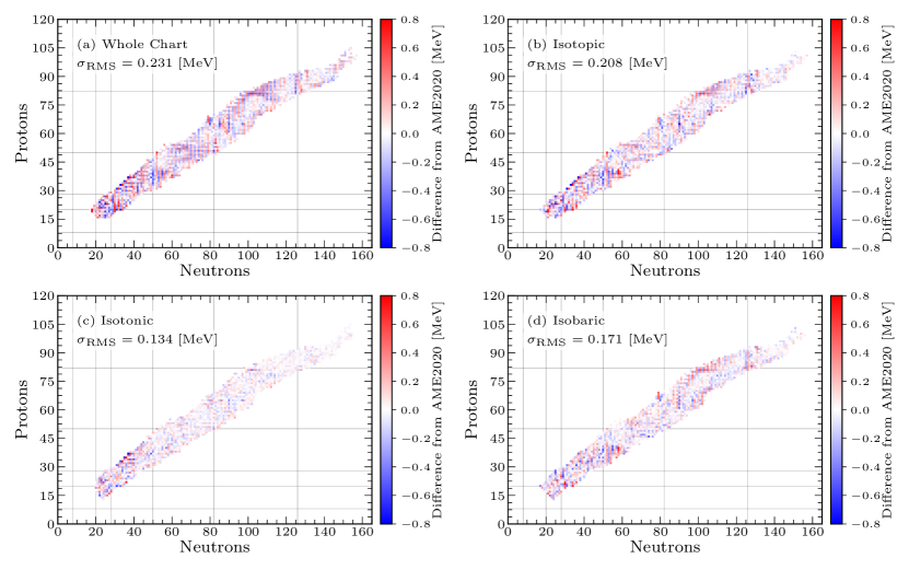
Figure 3: Deviation and root mean square (RMS) error $\sigma_{\text{RMS}}$ [MeV] of the neutron separation energies $S_{1n}$ reconstructed by the EBMA models fitted with (a) the whole chart of nuclides, (b) each isotopic chain ($Z=\text{const.}$), (c) each isotonic chain ($N=\text{const.}$), and (d) each isobaric chain ($A=\text{const.}$), compared to the AME2020 [20].

II.3 Setup of a numerical experiment

In the numerical experiments discussed in the current work, all probabilistic models have been implemented using PyMC [42], which is a probabilistic programming language written in Python. PyMC offers an implementation of a highly efficient sampler called No-U-Turn-Sampler (NUTS), which adaptively tunes the parameters associated with the Hamiltonian (or Hybrid) Monte Carlo method [43, 44]. Conventionally, parameter estimation in mixture models is performed with the Expectation Maximization (EM) algorithm to avoid the so-called “label switching problem” [45, 46]. The label switching problem arises in mixture models such as EBMA models, since the likelihood (Eq. 5) remains unchanged under permutation of the labels ($k=1,\;\ldots\;K$) of the mixture components $g_{k}(\Delta\mid m_{k})$. This makes the analysis of the posterior distributions challenging. Although, the EM algorithm does not guarantee convergence to the global optimal weights and variances, especially in high-dimensional problems.

Furthermore, MCMC methods would be able to provide much more complete information on the posterior distributions. In our numerical experiments, we did not find evidence of a label switching problem due to employing the MCMC method. This is most likely because, in our normal mixture models, the means of the normal distributions are always specified by the predictions of bias-corrected mass models, which works as an identifiability constraint.

The quantity of interest in our study is the one-neutron separation energy ($S_{1n}$), which is directly relevant to the $r$-process. In nucleosynthesis calculations (post-processing of hydrodynamical simulations), photodissociation rates (denoted as $\lambda_{(\gamma,n)}$ below) are often calculated from the neutron capture rate via detailed balance:

$$\lambda_{(\gamma,n)}= \expectationvalue{\sigma v}_{(n,\gamma)}\cdot\frac{G(N,Z)\cdot G(1,0)}{G(N+1,Z)}\cdot\left(\frac{A}{A+1}\right)^{3/2}$$

$$\cdot\left(\frac{m_{u}kT}{2\pi\hbar^{2}}\right)^{3/2}\cdot\exp\left(-\frac{S_{1n}(N+1,Z)}{kT}\right),$$ (8)

where $\expectationvalue{\sigma v}_{(n,\gamma)}$ is the velocity-integrated neutron capture cross section for a nucleus with $N$ neutrons and $Z$ protons ($A\equiv N+Z$), $G(N,Z)$ is the partition function for the nucleus $(N,Z)$ ($G(1,0)$ is the partition function for neutron), $m_{u}$ is the mass of a nucleon, and $T$ is the temperature of the environment. Note that the reverse rate is exponentially dependent on $S_{1n}$.

The mass models included in our ensembles are the Duflo-Zucker mass model with 29 parameters (DZ29) [7], FRDM2012 [2], HFB31 [10], KUTY05 [32], ETFSI2 [33], and WS4 [6]. In most of our numerical experiments, we take the $S_{1n}$ values from the AME2020 [20] as experimental data.

In evaluating the quality of uncertainty estimates for unseen data, we use the $S_{1n}$ values from the AME2003 [47] for constructing our models and then test them with the new data in the AME2020. In the AME2020, 319 new $S_{1n}$ measurements with $Z=16$–105 are available compared to the AME2003. The new data points in the AME2020 compared to the AME2003 are shown in Figure 2.

We consider four different ways to categorize the $S_{1n}$ data. The first category is the data for the whole chart of nuclides, which employs all the available experimental data at once. The second and third are data for each isotopic and isotonic chain, respectively. This focuses on the evolution of the $S_{1n}$ values as a function of proton and neutron number (isotopic and isotonic, respectively). The last is isobaric (equal mass number $A$), to demonstrate that it is possible to create an EBMA model for each isobaric chain, which is relevant to the trend of $\beta$-decay $Q$-values.

Table 2: 95 % posterior highest density intervals (HDI) of the EBMA weights and standard deviations (variances), fitted with the AME2020 $S_{1n}$ values. The notation $(a,b)$ denotes an interval with $a$ being the lower bound and $b$ being the upper bound, respectively. $\sigma_{RMS}$ (defined in Equation 9) shows the root mean square error of each mass model with respect to the AME2020 values.

Mass model	Weight	Standard deviation	$\sigma_{\text{RMS}}$ [MeV]
WS4	(0.392, 0.539)	(0.186, 0.221)	0.257
DZ29	(0.154, 0.277)	(0.134, 0.196)	0.292
FRDM12	(0.145, 0.264)	(0.143, 0.196)	0.350
KUTY05	(0.021, 0.127)	(0.134, 0.292)	0.746
ETFSI2	(0.001, 0.048)	(0.063, 0.450)	0.828
HFB31	(0.000, 0.029)	(0.138, 1.073)	0.472

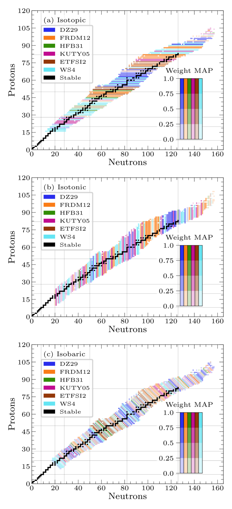
Figure 4: Maximum a posteriori (MAP) values of the largest weight in the EBMA ensemble determined for each (a) isotopic chain, (b) isotonic chain, and (c) isobaric chain.

III Results and Discussion

III.1 Comparison with observations

To compare the predictions of the EBMA model with the data from the AME2020, the nominal predictions of EBMA are taken as the MAP values of the predictive distributions of $S_{1n}$, with the bias-correction parameters, weights, and standard deviations $\sigma_{k}$ (Equation 3) also determined from the AME2020 values. Since the AME2020 values are used both for fitting and evaluation of the performance, this analysis reveals how well the EBMA method can reproduce known experimental data using the constituent mass models.

Figure 3 shows the deviations of the EBMA predictions of the one-neutron separation energies ($S_{1n}$) from the AME2020 values. The root mean square error ($\sigma_{\text{RMS}}$) shown in the figure is defined as

$$\sigma_{\text{RMS}}=\sqrt{\frac{\sum_{(N,Z)}\left(S_{1n}^{\text{AME2020}}{(N,Z)}-{S_{1n}^{\text{Model}}}{(N,Z)}\right)^{2}}{N^{\text{AME2020}}}},$$ (9)

where $(N,Z)$ represents pairs of neutron number $N$ and proton number $Z$ of nuclei in the AME2020 whose $S_{1n}$ values are used for the fit. $N^{\text{AME}}$ is the total number of such nuclei ($N^{\text{AME2020}}\equiv\sum_{(N,Z)}$). For the fit of the entire chart of nuclides, $N^{\text{AME2020}}=2030$. This number is slightly different in different fits, since some of the fits do not converge at the edge of the chart. $S_{1n}^{\text{AME2020}}(N,Z)$ and $S_{1n}^{\text{Model}}(N,Z)$ are the $S_{1n}$ values for a nucleus $(N,Z)$ from the AME2020 and mass models, respectively.

The value of $\sigma_{\text{RMS}}$ of the fit for the whole chart of nuclides (Figure 3 panel (a)) shows that the averaged mass model created by the EBMA method can reproduce the experimental values slightly better ($\sigma_{\mathrm{RMS}}^{\mathrm{(a)}}=0.231$ MeV) than the best performing model, which is the WS4 model [6] with $\sigma_{\mathrm{RMS}}^{\mathrm{WS4}}=0.257$ MeV (see Table 2). Further reduction in $\sigma_{\mathrm{RMS}}$ is achieved when $S_{1n}$ of each isotopic chain is fitted separately (panel (b) of Figure 3). This suggests that some models in the ensemble perform better than the overall best-performing mass model (WS4) for some isotopic chains. This can be verified by inspecting the weights of the EBMA model and will be discussed in more detail in the following Section III.2.

The best performance in reproducing the experimental $S_{1n}$ is obtained when separate EBMA models are optimized for each isotonic chain (panel (c) of Figure 3). This means that the mass models can capture the isotonic trends of $S_{1n}$ ($S_{1n}$ as function of the neutron number $N$) much better than the isotopic trends ($S_{1n}$ as function of the proton number $Z$), at least for the available experimental data. This is most likely because the values of $S_{1n}$ evolve rather smoothly as a function of the proton number, compared to as a function of the neutron number where odd-even staggering and the effect of neutron shell closures are present. The fit of each isobaric chain resulted in the RMS error value of 0.171 MeV, which sits between the isotopic and isotonic models (panel (d) of Figure 3).

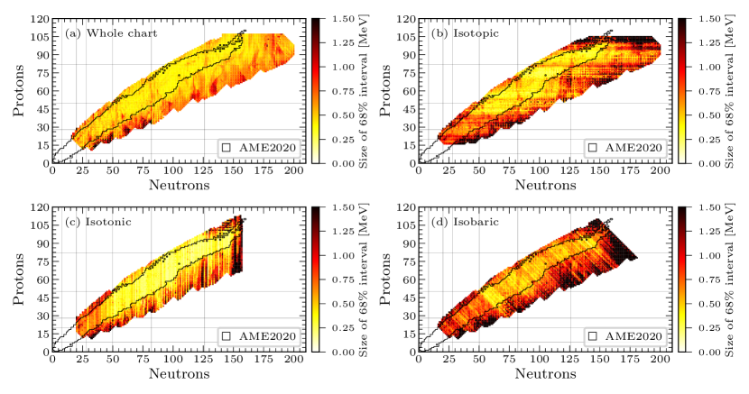
Figure 5: Trends of the sizes of 68% highest density intervals (HDIs) of the EBMA models, fitted with the AME2020 $S_{1n}$ data for (a) the whole chart of nuclides, (b) each isotopic chain, (c) each isotonic chain, and (d) each isobaric chain. The area enclosed by the black contour shows where the AME2020 data exist. The charts with isotonic and isobaric fits are truncated at a large neutron number and mass number, respectively, because there are not enough data points within the chains to determine the EBMA parameters.

III.2 Weights in the EBMA models

EBMA models are constructed using the $S_{1n}$ data from the AME2020 in three different ways: optimizing the EBMA models with the data for

1. the whole chart of nuclides,

2. each isotopic chain,

3. each isotonic chain, and

4. each isobaric chain,

respectively. Table 2 lists the 95 % posterior highest density intervals (HDIs) of the EBMA weights and variances, which are the narrowest intervals that include 95 % of the posterior distributions, when the EBMA model is optimized with the observed $S_{1n}$ data for the whole chart of nuclides.

The posterior weight, which can be interpreted as the probability of the model being the best one, is the largest for the WS4 model, followed by DZ29 and FRDM12. The order of the top three mass models is the same as the order of the smallest $\sigma_{\text{RMS}}$ errors with respect to the AME2020 [20].

On the other hand, the standard deviations or variances of the normal distributions in the mixture model do not follow the order of the $\sigma_{\text{RMS}}$ values. This is because the mixture model is a weighted sum of the normal distributions and is fitted to the data at once, not individually. It is not apparent why the posterior weight of the HFB31 model is much smaller than the others, even though the $\sigma_{\text{RMS}}$ value (0.472 MeV) is smaller than the KUTY05 (0.746 MeV) and ETFSI2 (0.828 MeV) models. The HFB31 mass model performs relatively well on average in reproducing the observed data, but it is possible that the local trend of the $S_{1n}$ values does not agree with the observation, therefore, resulting in a small weight. The size of the offset for the model compared to the AME2020 $S_{1n}$ data was the largest in the ensemble (Table 1), which may also suggest a systematic disagreement with the observations. Such disagreements could also explain the large interval of the posterior standard deviation of the model (Table 2).

The colors in Figure 4 show the mass model with the largest weight within the ensemble for each isotopic (panel (a)), isotonic (panel (b)), and isobaric chain (panel (c)). The color scale represents the value of the weight. The weight is the posterior probability of the mass model being the best one, based on the training using the AME2020 data. Trends of the best models in different regions are visible, especially when the ensembles are created for each isotopic chain. Note that the current method cannot provide explanations for why certain weights are large or small. Understanding the weights would require a careful analysis of the relative performance of each model.

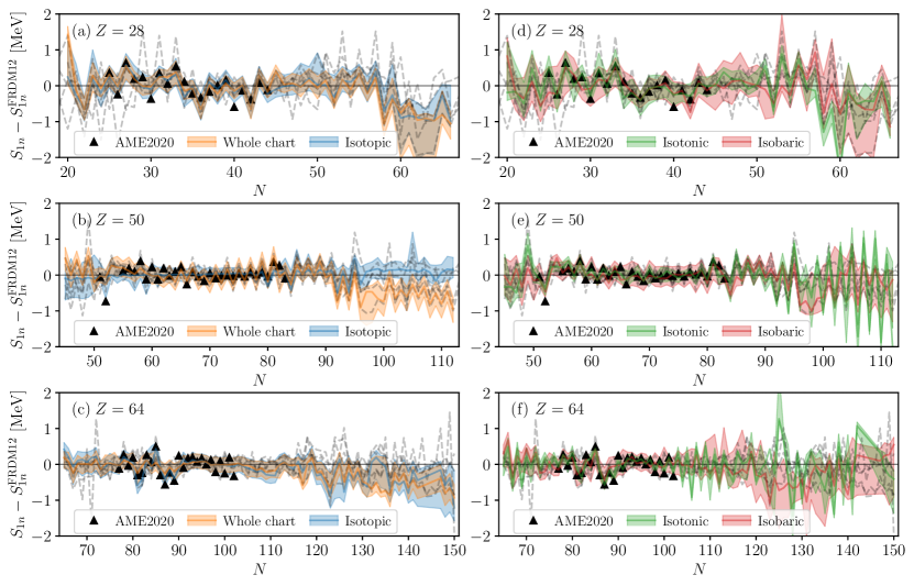
Figure 6: Trends of the sizes of 68% highest density intervals of the EBMA models for $Z=28$ (Ni) (panels (a) and (d)), $Z=50$ (Sn) (panels (b) and (e)), and $Z=64$ (Gd) (panels (c) and (f)) nuclei, similarly to Figure 1. Panels (a–c) show the EBMA models fitted with the AME2020 $S_{1n}$ data for the whole chart of nuclides (orange) and each isotopic chain (blue), and (d–f) show the models for each isotonic chain (green) and each isobaric chain (red). The gray dashed lines are the mass models shown in Figure 1.

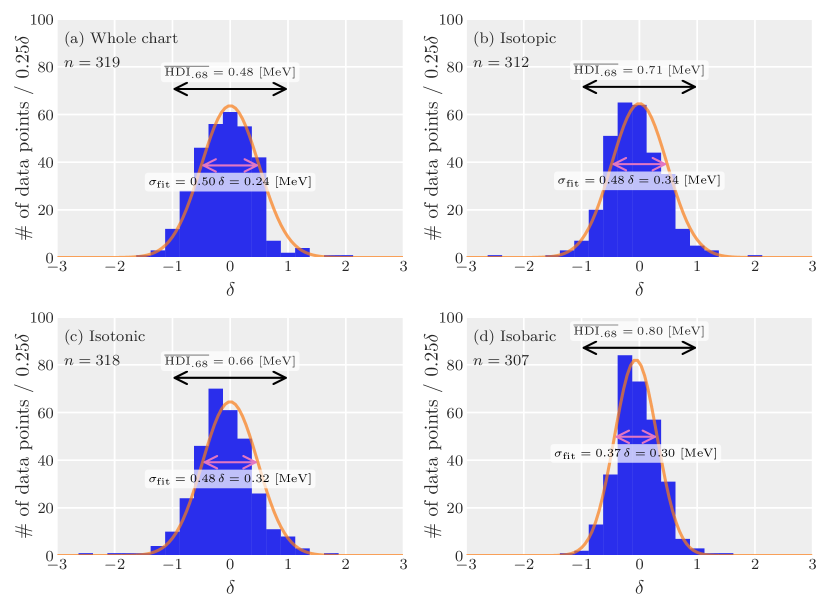
Figure 7: Distributions of the new data points in the AME2020 compared to the AME2003, with respect to the 68% HDIs predicted by the EBMA models fitted with the AME2003 data for (a) the whole chart of nuclides, (b) each isotopic chain, (c) each isotonic chain, and (d) each isobaric chain. The definition of $\delta$ is given in Equation 10.

III.3 Uncertainty quantification with EBMA

One of the main goals of this study is to quantify the uncertainty of the theoretical values $S_{1n}$ when a variety of mass models are available. EBMA estimates it by creating a weighted average of a collection of mass models, based on the performance of each model during the training. In the EBMA model, predictive uncertainty includes not only the spread of the forecasts among the members of the ensemble, but also takes into account the weighted variance of each member model according to the performance during the training [21]. The interpretability of the uncertainty is another advantage of the EBMA method.

III.3.1 Size of uncertainty estimates

Figure 5 shows the size of the 68% highest density interval (HDI), which is roughly comparable to the $\pm 1\sigma$ interval of the normal distribution, with EBMA models fitted for the whole chart of nuclides (panel (a)), each isotopic chain (panel (b)), each isotonic chain (panel (c)), and each isobaric chain (panel (d)), respectively. Figure 6 also shows the 68% HDIs, focusing on the $Z=28$ (nickel), $Z=50$ (tin), and $Z=64$ (gadolinium) isotopes, compared to the mass models (gray dashed lines) shown in Figure 1. The panels (a)–(c) show the EBMA models fitted for the whole chart of nuclides and each isotopic chain and (d)–(f) show the models for each isotopic chain and each isobaric chain for the same set of nuclei. The fits are performed using the AME2020 data, and the predictions are made for all the nuclei available in all the member mass models within the ensemble. In all the cases, it can be seen that the size of the uncertainty is constrained where the data exist (black contour in Figure 5), but increases towards the edge of the chart of nuclides, especially in the neutron-rich direction. This reflects the fact that the predictions of the mass models constituting the ensemble start to diverge as we move further away from the last data point, as shown in Figure 1.

Comparing the four plots of Figure 5, the increase in the size of uncertainty in the neutron-rich region is the smallest for the fit using the whole chart of nuclides (panel (a)). This is likely because the weights for the whole chart of nuclides can be determined using all available data, whereas for each isotopic, isotonic, and isobaric chain, respectively, the weights are determined only from the data in each chain. Although the isotonic fit was best performing in terms of reproducing the experimental data (Figure 3), it can be seen from the panel (c) of Figure 5, the size of uncertainty rapidly grows where no experimental data exist.

These results show that, in general, the current theoretical understanding and the accuracy of modeling of nuclear masses become increasingly uncertain towards the neutron-rich region. Therefore, in investigating the impact of uncertain masses on the prediction of the $r$-process observables, such an increase in the size of uncertainty should be taken into account. Using the EBMA uncertainty would allow for more realistic uncertainty quantification and sensitivity studies of the $r$-process observables.

III.3.2 Quality of uncertainty estimates

As discussed in Section II.2, the predictive uncertainty given by the EBMA model has a straightforward interpretation. Now, we investigate the quality of the estimation of the size of uncertainty. We first construct EBMA models and quantify the prediction uncertainties using the data from the AME2003 [47], then evaluate the quality of the uncertainties based on the new data from the AME2020 [20].

Figure 7 shows the distribution of the new $S_{1n}$ data relative to the sizes of uncertainties given by the EBMA models fitted with the data for the whole chart of nuclides (panel (a)), fitted for each isotopic chain (panel (b)), isotonic chain (panel (c)), and isobaric chain (panel (d)). The number of new data points included in the fit ($n$ in Figure 7) is not necessarily 319 for the isotopic/isotonic/isobaric fits because at the edge of the chart of nuclides, often there are not enough data points in the isotopic/isotonic/isobaric chains and the posterior weights do not converge. Such data points are excluded from the fits.

The size of the EBMA uncertainty is taken as the 68% highest (posterior) density interval (HDI_.68), which is the narrowest 68% credible interval on the posterior distribution. If the distribution is a perfect normal distribution, 68% corresponds to the $\pm 1\sigma$ interval symmetric about the mean. To study how the observation distributes relatively to the HDI_.68, we define $\delta$, which represents an observed $S_{1n}$ value normalized by the size of HDI_.68. Let $h^{\mathrm{low}}$ and $h^{\mathrm{up}}$ represent the lower and upper boundaries of the HDI_.68, respectively,

$$\delta=\frac{S_{1n}-h^{\mathrm{low}}}{h^{\mathrm{up}}-h^{\mathrm{low}}}-0.5,$$ (10)

where 0.5 is subtracted to symmetrize the distribution around 0. This means that $\delta=-1$ and $1$ correspond to the $S_{1n}$ values at the lower and upper boundaries of the HDI_.68, respectively.

Comparing the average sizes of the 68% intervals ($\overline{\mathrm{HDI}_{.68}}$), on average, the model fitted with the whole chart of nuclides (panel (a) of Figure 7) provides the most constrained size of the uncertainty of 0.48 MeV. On the other hand, the models fitted for each isotopic (panel (b)), isotonic (panel (c)), and isobaric (panel (d)) chain have larger credible intervals. This is most likely due to the fewer observation data points in each isotopic, isotonic, or isobaric chain compared to the data for the whole chart of nuclides. For the isotopic and isotonic fits (panels (c) and (d)), some data points around $\delta\sim 2$ can be seen, suggesting that the models optimized for isotopic/isotonic chains may be more sensitive to observations that do not follow the trend within the isotopic/isotonic chain. This means that the isotopic/isotonic models may be used to detect anomalous masses or separation energies with respect to the trend within the isotopic/isotonic chain. Since most of the new data points fall within the 68 % intervals, while the sizes of the uncertainties are somewhat overestimated, it can be concluded that the EBMA method is capable of extrapolating the $S_{1n}$ values with conservative uncertainty estimates, when the new data points are adjacent to the existing data. The quantified uncertainties may also be used to estimate the probabilities of certain nuclei to be bound as in Refs. [25, 36, 48], which will be addressed in future work.

IV Conclusions

We have explored the possibility of quantifying the uncertainty of theoretical one-neutron separation energies ($S_{1n}$) when a variety of mass models are available, using the Ensemble Baysian Model Averaging (EBMA) method. The EBMA method models an ensemble of bias-corrected mass models as a mixture of normal distributions, whose parameters are estimated by MCMC using the No-U-Turn-Sampler (NUTS). EBMA models have been constructed in four different ways of fitting, namely, the whole chart of nuclides, each isotopic chain, each isotonic chain, and each isobaric chain.

In reproducing the observed one-neutron separation energies ($S_{1n}$), in all cases, the maximum a posteriori (MAP) estimates of the EBMA models result in smaller root mean square deviations from the AME2020 data than the best model in the ensemble, namely the WS4 model ($\sigma_{\text{RMS}}^{\text{WS4}}=0.257$ [MeV]). While the EBMA model fitted for the whole chart of nuclides results in a larger $\sigma_{\mathrm{RMS}}$ value than the isotopic/isotonic/isobaric fit, it provides a more constrained and accurate uncertainty.

For all cases, the 68% HDIs estimated from the AME2003 data contain roughly 95% of the new observations in the AME2020. This suggests that the extrapolations of the $S_{1n}$ values provided by the current EBMA models based on the AME2003 data and the six theoretical mass models work well for the new data in the AME2020. Furthermore, based on the distributions of the new AME2020 data with respect to the size of the 68% HDIs, we conclude that the EBMA method provides meaningful but conservative uncertainty estimates.

The advantage of the EBMA method is its simplicity in obtaining the uncertainty estimates of an ensemble of theoretical models. This would make it possible to apply the current method to various nuclear physics observables. Using an ensemble of theoretical models can also naturally model the fact that the predictions of nuclear physics models are not well constrained far from stability, especially in the neutron-rich region. Such realistic uncertainty estimates are necessary to accurately assess the impact of uncertain nuclear physics inputs in the studies of heavy element nucleosynthesis, especially the $r$-process.