For a basis { p 1 , ⋯ , p N } subscript 𝑝 1 ⋯ subscript 𝑝 𝑁 \{p_{1},\cdots,p_{N}\} 𝒫 n ( ℝ d ) subscript 𝒫 𝑛 superscript ℝ 𝑑 {\cal P}_{n}(\mathbb{R}^{d}) N 𝑁 N 𝐱 1 , ⋯ , 𝐱 N subscript 𝐱 1 ⋯ subscript 𝐱 𝑁
{\bf x}_{1},\cdots,{\bf x}_{N} K 𝐾 K
vdm ( 𝐱 1 , ⋯ , 𝐱 N ) := det ( [ p j ( 𝐱 i ) ] 1 ≤ i , j ≤ N ) . assign vdm subscript 𝐱 1 ⋯ subscript 𝐱 𝑁 det subscript delimited-[] subscript 𝑝 𝑗 subscript 𝐱 𝑖 formulae-sequence 1 𝑖 𝑗 𝑁 {\rm vdm}({\bf x}_{1},\cdots,{\bf x}_{N}):={\rm det}([p_{j}({\bf x}_{i})]_{1\leq i,j\leq N}).
In case the Vandermonde determinant is non-zero, the problem of interpolation at these points by polynomials of degree at most n 𝑛 n ℓ i ( 𝐱 ) subscript ℓ 𝑖 𝐱 \ell_{i}({\bf x}) n 𝑛 n
ℓ i ( 𝐱 j ) = δ i j . subscript ℓ 𝑖 subscript 𝐱 𝑗 subscript 𝛿 𝑖 𝑗 \ell_{i}({\bf x}_{j})=\delta_{ij}.
In the case that K ⊂ ℝ d 𝐾 superscript ℝ 𝑑 K\subset\mathbb{R}^{d} [2 ] that, for X 𝑋 X n 𝑛 n independent of the dimension. Specifically,
Λ n ( X ; K ) ≤ ( 2 n − 1 n ) , ∀ d ≥ 1 . formulae-sequence subscript Λ 𝑛 𝑋 𝐾
binomial 2 𝑛 1 𝑛 for-all 𝑑 1 \Lambda_{n}(X;K)\leq{2n-1\choose n},\quad\forall d\geq 1.
It follows that there is also such a bound for the Lebesgue points, i.e. those for which the Lebesgue constant is a minimum (and hence also highle likely for any good set of interpolation points).
The subject of this short paper is to study the growth as a function of the dimension d , 𝑑 d, of Λ n ( X ) subscript Λ 𝑛 𝑋 \Lambda_{n}(X) n = 1 𝑛 1 n=1 X 𝑋 X K 𝐾 K
In the degree one case we have N 1 = d + 1 subscript 𝑁 1 𝑑 1 N_{1}=d+1 X = { 𝐱 1 , ⋯ , 𝐱 N } ⊂ ℝ d 𝑋 subscript 𝐱 1 ⋯ subscript 𝐱 𝑁 superscript ℝ 𝑑 X=\{{\bf x}_{1},\cdots,{\bf x}_{N}\}\subset\mathbb{R}^{d}
𝐱 i = ( x 1 ( i ) , x 2 ( i ) , ⋯ , x d ( i ) ) ∈ ℝ d subscript 𝐱 𝑖 subscript superscript 𝑥 𝑖 1 subscript superscript 𝑥 𝑖 2 ⋯ subscript superscript 𝑥 𝑖 𝑑 superscript ℝ 𝑑 {\bf x}_{i}=(x^{(i)}_{1},x^{(i)}_{2},\cdots,x^{(i)}_{d})\in\mathbb{R}^{d}
the Vandermonde determinant for the basis of monomials { x 1 , x 2 , ⋯ , x d } subscript 𝑥 1 subscript 𝑥 2 ⋯ subscript 𝑥 𝑑 \{x_{1},x_{2},\cdots,x_{d}\}
vdm ( 𝐱 1 , ⋯ , 𝐱 d ) = | 1 x 1 ( 1 ) x 2 ( 1 ) ⋅ ⋅ x d ( 1 ) 1 x 1 ( 2 ) x 2 ( 2 ) ⋅ ⋅ x d ( 2 ) ⋅ ⋅ ⋅ ⋅ 1 x 1 ( d ) x 2 ( d ) ⋅ ⋅ x d ( d ) 1 x 1 ( d + 1 ) x 2 ( d + 1 ) ⋅ ⋅ x d ( d + 1 ) | vdm subscript 𝐱 1 ⋯ subscript 𝐱 𝑑 1 superscript subscript 𝑥 1 1 superscript subscript 𝑥 2 1 ⋅ ⋅ superscript subscript 𝑥 𝑑 1 1 superscript subscript 𝑥 1 2 superscript subscript 𝑥 2 2 ⋅ ⋅ superscript subscript 𝑥 𝑑 2 ⋅ missing-subexpression missing-subexpression missing-subexpression missing-subexpression ⋅ ⋅ missing-subexpression missing-subexpression missing-subexpression missing-subexpression ⋅ 1 superscript subscript 𝑥 1 𝑑 superscript subscript 𝑥 2 𝑑 ⋅ ⋅ superscript subscript 𝑥 𝑑 𝑑 1 superscript subscript 𝑥 1 𝑑 1 superscript subscript 𝑥 2 𝑑 1 ⋅ ⋅ superscript subscript 𝑥 𝑑 𝑑 1 {\rm vdm}({\bf x}_{1},\cdots,{\bf x}_{d})=\left|\begin{array}[]{cccccc}1&x_{1}^{(1)}&x_{2}^{(1)}&\cdot&\cdot&x_{d}^{(1)}\cr 1&x_{1}^{(2)}&x_{2}^{(2)}&\cdot&\cdot&x_{d}^{(2)}\cr\cdot&&&&&\cdot\cr\cdot&&&&&\cdot\cr 1&x_{1}^{(d)}&x_{2}^{(d)}&\cdot&\cdot&x_{d}^{(d)}\cr 1&x_{1}^{(d+1)}&x_{2}^{(d+1)}&\cdot&\cdot&x_{d}^{(d+1)}\end{array}\right|
which equals ± d ! plus-or-minus 𝑑 \pm d! X . 𝑋 X. K . 𝐾 K.
2 K 𝐾 K
We construct recusrsively the d + 1 𝑑 1 d+1 ℝ d superscript ℝ 𝑑 \mathbb{R}^{d}
X 1 = [ − 1 + 1 ] ∈ ℝ 2 × 1 . subscript 𝑋 1 delimited-[] 1 1 superscript ℝ 2 1 X_{1}=\left[\begin{array}[]{l}-1\cr+1\end{array}\right]\in\mathbb{R}^{2\times 1}.
Then, for d > 1 𝑑 1 d>1 X d − 1 ∈ R d × ( d − 1 ) , subscript 𝑋 𝑑 1 superscript 𝑅 𝑑 𝑑 1 X_{d-1}\in R^{d\times(d-1)},
X d := [ − 1 / d R d X d − 1 − 1 / d − 1 / d 0 ⋅ 0 1 ] ∈ ℝ ( d + 1 ) × d assign subscript 𝑋 𝑑 delimited-[] missing-subexpression missing-subexpression missing-subexpression 1 𝑑 missing-subexpression subscript 𝑅 𝑑 subscript 𝑋 𝑑 1 missing-subexpression 1 𝑑 missing-subexpression missing-subexpression missing-subexpression 1 𝑑 0 ⋅ 0 1 superscript ℝ 𝑑 1 𝑑 X_{d}:=\left[\begin{array}[]{cccc}&&&-1/d\cr&R_{d}X_{d-1}&&-1/d\cr&&&-1/d\cr 0&\cdot&0&1\end{array}\right]\in\mathbb{R}^{(d+1)\times d}
where
R d := d 2 − 1 d . assign subscript 𝑅 𝑑 superscript 𝑑 2 1 𝑑 R_{d}:=\frac{\sqrt{d^{2}-1}}{d}.
Each row of X d subscript 𝑋 𝑑 X_{d} ℝ d . superscript ℝ 𝑑 \mathbb{R}^{d}. X d subscript 𝑋 𝑑 X_{d} X d − 1 , subscript 𝑋 𝑑 1 X_{d-1}, ℝ d − 1 superscript ℝ 𝑑 1 \mathbb{R}^{d-1} ℝ d superscript ℝ 𝑑 \mathbb{R}^{d} x d = − 1 / d subscript 𝑥 𝑑 1 𝑑 x_{d}=-1/d ( 0 , ⋯ , 0 , 1 ) ∈ ℝ d . 0 ⋯ 0 1 superscript ℝ 𝑑 (0,\cdots,0,1)\in\mathbb{R}^{d}.
Lemma 2.1 .
The centroid of the points gievn by X d subscript 𝑋 𝑑 X_{d} 𝟎 d ∈ ℝ d , subscript 0 𝑑 superscript ℝ 𝑑 {\bm{0}}_{d}\in\mathbb{R}^{d}, X d t 𝟙 d + 1 = 𝟎 d . superscript subscript 𝑋 𝑑 𝑡 subscript 1 𝑑 1 subscript 0 𝑑 X_{d}^{t}{\mathbbm{1}}_{d+1}={\bm{0}}_{d}.
Proof (by induction on d 𝑑 d d = 1 , 𝑑 1 d=1,
X 1 t 𝟙 2 = [ − 1 1 ] [ 1 1 ] = 0 . superscript subscript 𝑋 1 𝑡 subscript 1 2 delimited-[] 11 delimited-[] 1 1 0 X_{1}^{t}\mathbbm{1}_{2}=[-1\,\,1]\left[\begin{array}[]{c}1\cr 1\end{array}\right]=0.
Hence assume that X d − 1 t 𝟙 d = 𝟎 d − 1 superscript subscript 𝑋 𝑑 1 𝑡 subscript 1 𝑑 subscript 0 𝑑 1 X_{d-1}^{t}\mathbbm{1}_{d}={\bm{0}}_{d-1}
X d t 𝟙 d + 1 superscript subscript 𝑋 𝑑 𝑡 subscript 1 𝑑 1 \displaystyle X_{d}^{t}\mathbbm{1}_{d+1} = [ 0 R d X d − 1 t 0 0 − 1 / d ⋅ − 1 / d 1 ] [ 1 ⋅ ⋅ 1 ] absent delimited-[] missing-subexpression missing-subexpression missing-subexpression 0 missing-subexpression subscript 𝑅 𝑑 superscript subscript 𝑋 𝑑 1 𝑡 missing-subexpression 0 missing-subexpression missing-subexpression missing-subexpression 0 1 𝑑 ⋅ 1 𝑑 1 delimited-[] 1 ⋅ ⋅ 1 \displaystyle=\left[\begin{array}[]{cccc}&&&0\cr&R_{d}X_{d-1}^{t}&&0\cr&&&0\cr-1/d&\cdot&-1/d&1\end{array}\right]\,\left[\begin{array}[]{c}1\cr\cdot\cr\cdot\cr 1\end{array}\right]
= [ R d X d − 1 t 𝟙 d d ( − 1 / d ) + 1 ] absent delimited-[] subscript 𝑅 𝑑 superscript subscript 𝑋 𝑑 1 𝑡 subscript 1 𝑑 𝑑 1 𝑑 1 \displaystyle=\left[\begin{array}[]{c}R_{d}X_{d-1}^{t}\mathbbm{1}_{d}\cr d(-1/d)+1\end{array}\right]
= 𝟎 d . absent subscript 0 𝑑 \displaystyle={\bm{0}}_{d}.
□ □ \square
Lemma 2.2 .
We have
X d t X d = d + 1 d I d . superscript subscript 𝑋 𝑑 𝑡 subscript 𝑋 𝑑 𝑑 1 𝑑 subscript 𝐼 𝑑 X_{d}^{t}X_{d}=\frac{d+1}{d}I_{d}.
Proof (by induction on the dimension d 𝑑 d d = 1 , 𝑑 1 d=1,
X 1 t X 1 = [ − 1 1 ] [ − 1 + 1 ] = 2 = 1 + 1 1 I 1 . superscript subscript 𝑋 1 𝑡 subscript 𝑋 1 delimited-[] 11 delimited-[] 1 1 2 1 1 1 subscript 𝐼 1 X_{1}^{t}X_{1}=[-1\,\,1]\left[\begin{array}[]{c}-1\cr+1\end{array}\right]=2=\frac{1+1}{1}I_{1}.
Assume then the Lemma holds for dimension d − 1 . 𝑑 1 d-1.
X d t X d superscript subscript 𝑋 𝑑 𝑡 subscript 𝑋 𝑑 \displaystyle X_{d}^{t}X_{d} = [ 0 R d X d − 1 t 0 0 − 1 / d ⋅ − 1 / d 1 ] [ − 1 / d R d X d − 1 − 1 / d − 1 / d 0 ⋅ 0 1 ] absent delimited-[] missing-subexpression missing-subexpression missing-subexpression 0 missing-subexpression subscript 𝑅 𝑑 superscript subscript 𝑋 𝑑 1 𝑡 missing-subexpression 0 missing-subexpression missing-subexpression missing-subexpression 0 1 𝑑 ⋅ 1 𝑑 1 delimited-[] missing-subexpression missing-subexpression missing-subexpression 1 𝑑 missing-subexpression subscript 𝑅 𝑑 subscript 𝑋 𝑑 1 missing-subexpression 1 𝑑 missing-subexpression missing-subexpression missing-subexpression 1 𝑑 0 ⋅ 0 1 \displaystyle=\left[\begin{array}[]{cccc}&&&0\cr&R_{d}X_{d-1}^{t}&&0\cr&&&0\cr-1/d&\cdot&-1/d&1\end{array}\right]\,\left[\begin{array}[]{cccc}&&&-1/d\cr&R_{d}X_{d-1}&&-1/d\cr&&&-1/d\cr 0&\cdot&0&1\end{array}\right]
= [ R d 2 X d − 1 t X d − 1 R d X d − 1 t [ − 1 / d ⋅ ⋅ − 1 / d ] [ − 1 / d ⋅ ⋅ − 1 / d ] R d X d − 1 d d 2 + 1 ] \displaystyle=\left[\begin{array}[]{cc}R_{d}^{2}X_{d-1}^{t}X_{d-1}&R_{d}X_{d-1}^{t}\left[\begin{array}[]{c}-1/d\cr\cdot\cr\cdot\cr-1/d\end{array}\right]\cr\bigl{[}-1/d\,\cdot\,\cdot\,-1/d\bigr{]}R_{d}X_{d-1}&\frac{d}{d^{2}}+1\end{array}\right]
= [ d 2 − 1 d 2 d d − 1 I d − 1 𝟎 d − 1 𝟎 d − 1 t 1 + 1 / d ] absent delimited-[] superscript 𝑑 2 1 superscript 𝑑 2 𝑑 𝑑 1 subscript 𝐼 𝑑 1 subscript 0 𝑑 1 subscript superscript 0 𝑡 𝑑 1 1 1 𝑑 \displaystyle=\left[\begin{array}[]{cc}\frac{d^{2}-1}{d^{2}}\,\frac{d}{d-1}I_{d-1}&{\bm{0}}_{d-1}\cr{\bm{0}}^{t}_{d-1}&1+1/d\end{array}\right]
= d + 1 d I d absent 𝑑 1 𝑑 subscript 𝐼 𝑑 \displaystyle=\frac{d+1}{d}I_{d}
as
X d − 1 t [ − 1 / d ⋅ ⋅ − 1 / d ] = − 1 d X d − 1 t [ 1 ⋅ ⋅ 1 ] = 𝟎 d − 1 superscript subscript 𝑋 𝑑 1 𝑡 delimited-[] 1 𝑑 ⋅ ⋅ 1 𝑑 1 𝑑 superscript subscript 𝑋 𝑑 1 𝑡 delimited-[] 1 ⋅ ⋅ 1 subscript 0 𝑑 1 X_{d-1}^{t}\left[\begin{array}[]{c}-1/d\cr\cdot\cr\cdot\cr-1/d\end{array}\right]=-\frac{1}{d}X_{d-1}^{t}\left[\begin{array}[]{c}1\cr\cdot\cr\cdot\cr 1\end{array}\right]={\bm{0}}_{d-1}
by Lemma 2.1 □ □ \square
Lemma 2.3 .
We have
X d X d t = d + 1 d I d + 1 − 1 d 𝟙 d + 1 𝟙 d + 1 t ∈ ℝ ( d + 1 ) × ( d + 1 ) . subscript 𝑋 𝑑 superscript subscript 𝑋 𝑑 𝑡 𝑑 1 𝑑 subscript 𝐼 𝑑 1 1 𝑑 subscript 1 𝑑 1 superscript subscript 1 𝑑 1 𝑡 superscript ℝ 𝑑 1 𝑑 1 X_{d}X_{d}^{t}=\frac{d+1}{d}I_{d+1}-\frac{1}{d}\mathbbm{1}_{d+1}\mathbbm{1}_{d+1}^{t}\in\mathbb{R}^{(d+1)\times(d+1)}.
Proof (by induction on the dimension d 𝑑 d d = 1 , 𝑑 1 d=1,
X 1 X 1 t subscript 𝑋 1 superscript subscript 𝑋 1 𝑡 \displaystyle X_{1}X_{1}^{t} = [ − 1 + 1 ] [ − 1 + 1 ] = [ + 1 − 1 − 1 + 1 ] absent delimited-[] 1 1 delimited-[] 1 1 delimited-[] 1 1 1 1 \displaystyle=\left[\begin{array}[]{c}-1\cr+1\end{array}\right]\,[-1\,\,+1]=\left[\begin{array}[]{cc}+1&-1\cr-1&+1\end{array}\right]
= [ 2 0 0 2 ] − [ 1 1 1 1 ] absent delimited-[] 2 0 0 2 delimited-[] 1 1 1 1 \displaystyle=\left[\begin{array}[]{cc}2&0\cr 0&2\end{array}\right]-\left[\begin{array}[]{cc}1&1\cr 1&1\end{array}\right]
= 1 + 1 1 I 2 − 1 1 𝟙 2 𝟙 2 t . absent 1 1 1 subscript 𝐼 2 1 1 subscript 1 2 superscript subscript 1 2 𝑡 \displaystyle=\frac{1+1}{1}I_{2}-\frac{1}{1}\mathbbm{1}_{2}\mathbbm{1}_{2}^{t}.
Hence assume that the Lemma holds for d − 1 . 𝑑 1 d-1.
X d X d t subscript 𝑋 𝑑 superscript subscript 𝑋 𝑑 𝑡 \displaystyle X_{d}X_{d}^{t} = [ − 1 / d R d X d − 1 − 1 / d − 1 / d 0 ⋅ 0 1 ] [ 0 R d X d − 1 t 0 0 − 1 / d ⋅ − 1 / d 1 ] absent delimited-[] missing-subexpression missing-subexpression missing-subexpression 1 𝑑 missing-subexpression subscript 𝑅 𝑑 subscript 𝑋 𝑑 1 missing-subexpression 1 𝑑 missing-subexpression missing-subexpression missing-subexpression 1 𝑑 0 ⋅ 0 1 delimited-[] missing-subexpression missing-subexpression missing-subexpression 0 missing-subexpression subscript 𝑅 𝑑 superscript subscript 𝑋 𝑑 1 𝑡 missing-subexpression 0 missing-subexpression missing-subexpression missing-subexpression 0 1 𝑑 ⋅ 1 𝑑 1 \displaystyle=\left[\begin{array}[]{cccc}&&&-1/d\cr&R_{d}X_{d-1}&&-1/d\cr&&&-1/d\cr 0&\cdot&0&1\end{array}\right]\,\left[\begin{array}[]{cccc}&&&0\cr&R_{d}X_{d-1}^{t}&&0\cr&&&0\cr-1/d&\cdot&-1/d&1\end{array}\right]
= [ R d 2 X d − 1 X d − 1 t + 1 d 2 𝟙 d 𝟙 d t − 1 / d ⋅ ⋅ − 1 / d − 1 / d ⋅ ⋅ − 1 / d 1 ] absent delimited-[] superscript subscript 𝑅 𝑑 2 subscript 𝑋 𝑑 1 superscript subscript 𝑋 𝑑 1 𝑡 1 superscript 𝑑 2 subscript 1 𝑑 superscript subscript 1 𝑑 𝑡 1 𝑑 ⋅ ⋅ 1 𝑑 1 𝑑 ⋅ ⋅ 1 𝑑 1 \displaystyle=\left[\begin{array}[]{cc}R_{d}^{2}X_{d-1}X_{d-1}^{t}+\frac{1}{d^{2}}\mathbbm{1}_{d}\mathbbm{1}_{d}^{t}&\begin{array}[]{c}-1/d\cr\cdot\cr\cdot\cr-1/d\end{array}\cr\begin{array}[]{cccc}-1/d&\cdot&\cdot&-1/d\end{array}&1\end{array}\right]
= [ d 2 − 1 d 2 ( d d − 1 I d − 1 d − 1 𝟙 d 𝟙 d t ) + 1 d 2 𝟙 d 𝟙 d t − 1 / d ⋅ ⋅ − 1 / d − 1 / d ⋅ ⋅ − 1 / d 1 ] absent delimited-[] superscript 𝑑 2 1 superscript 𝑑 2 𝑑 𝑑 1 subscript 𝐼 𝑑 1 𝑑 1 subscript 1 𝑑 superscript subscript 1 𝑑 𝑡 1 superscript 𝑑 2 subscript 1 𝑑 superscript subscript 1 𝑑 𝑡 1 𝑑 ⋅ ⋅ 1 𝑑 1 𝑑 ⋅ ⋅ 1 𝑑 1 \displaystyle=\left[\begin{array}[]{cc}\frac{d^{2}-1}{d^{2}}\Bigl{(}\frac{d}{d-1}I_{d}-\frac{1}{d-1}\mathbbm{1}_{d}\mathbbm{1}_{d}^{t}\Bigr{)}+\frac{1}{d^{2}}\mathbbm{1}_{d}\mathbbm{1}_{d}^{t}&\begin{array}[]{c}-1/d\cr\cdot\cr\cdot\cr-1/d\end{array}\cr\begin{array}[]{cccc}-1/d&\cdot&\cdot&-1/d\end{array}&1\end{array}\right]
= [ d + 1 d I d − 1 d 𝟙 d 𝟙 d t − 1 / d ⋅ ⋅ − 1 / d − 1 / d ⋅ ⋅ − 1 / d 1 ] absent delimited-[] 𝑑 1 𝑑 subscript 𝐼 𝑑 1 𝑑 subscript 1 𝑑 superscript subscript 1 𝑑 𝑡 1 𝑑 ⋅ ⋅ 1 𝑑 1 𝑑 ⋅ ⋅ 1 𝑑 1 \displaystyle=\left[\begin{array}[]{cc}\frac{d+1}{d}I_{d}-\frac{1}{d}\mathbbm{1}_{d}\mathbbm{1}_{d}^{t}&\begin{array}[]{c}-1/d\cr\cdot\cr\cdot\cr-1/d\end{array}\cr\begin{array}[]{cccc}-1/d&\cdot&\cdot&-1/d\end{array}&1\end{array}\right]
= d + 1 d I d + 1 − 1 d 𝟙 d + 1 𝟙 d + 1 t . absent 𝑑 1 𝑑 subscript 𝐼 𝑑 1 1 𝑑 subscript 1 𝑑 1 superscript subscript 1 𝑑 1 𝑡 \displaystyle=\frac{d+1}{d}I_{d+1}-\frac{1}{d}\mathbbm{1}_{d+1}\mathbbm{1}_{d+1}^{t}.
□ □ \square
Remark . The matrix X d X d t subscript 𝑋 𝑑 superscript subscript 𝑋 𝑑 𝑡 X_{d}X_{d}^{t} X d . subscript 𝑋 𝑑 X_{d}. 1 1 1 − 1 / d 1 𝑑 -1/d 𝐱 i subscript 𝐱 𝑖 {\bf x}_{i} 𝐱 j subscript 𝐱 𝑗 {\bf x}_{j}
‖ 𝐱 i − 𝐱 j ‖ 2 2 superscript subscript norm subscript 𝐱 𝑖 subscript 𝐱 𝑗 2 2 \displaystyle\|{\bf x}_{i}-{\bf x}_{j}\|_{2}^{2} = ( 𝐱 i − 𝐱 j ) t ( 𝐱 i − 𝐱 j ) absent superscript subscript 𝐱 𝑖 subscript 𝐱 𝑗 𝑡 subscript 𝐱 𝑖 subscript 𝐱 𝑗 \displaystyle=({\bf x}_{i}-{\bf x}_{j})^{t}({\bf x}_{i}-{\bf x}_{j})
= 𝐱 i t 𝐱 j − 2 𝐱 i 𝐱 j + 𝐱 j t 𝐱 j absent superscript subscript 𝐱 𝑖 𝑡 subscript 𝐱 𝑗 2 subscript 𝐱 𝑖 subscript 𝐱 𝑗 superscript subscript 𝐱 𝑗 𝑡 subscript 𝐱 𝑗 \displaystyle={\bf x}_{i}^{t}{\bf x}_{j}-2{\bf x}_{i}{\bf x}_{j}+{\bf x}_{j}^{t}{\bf x}_{j}
= 1 − 2 ( − 1 / d ) + 1 = 2 d + 1 d , ∀ i ≠ j . formulae-sequence absent 1 2 1 𝑑 1 2 𝑑 1 𝑑 for-all 𝑖 𝑗 \displaystyle=1-2(-1/d)+1=2\frac{d+1}{d},\quad\forall i\neq j.
□ □ \square
The barycentric coordinates of 𝐲 ∈ ℝ d 𝐲 superscript ℝ 𝑑 {\bf y}\in\mathbb{R}^{d} X d subscript 𝑋 𝑑 X_{d} 𝝀 ∈ ℝ d + 1 𝝀 superscript ℝ 𝑑 1 {\bm{\lambda}}\in\mathbb{R}^{d+1}
(a) X d t 𝝀 = 𝐲 , superscript subscript 𝑋 𝑑 𝑡 𝝀 𝐲 X_{d}^{t}{\bm{\lambda}}={\bf y},
(b) 𝟙 d + 1 t 𝝀 = 1 . superscript subscript 1 𝑑 1 𝑡 𝝀 1 \mathbbm{1}_{d+1}^{t}{\bm{\lambda}}=1.
Lemma 2.4 .
We have, for 𝐲 ∈ ℝ d , 𝐲 superscript ℝ 𝑑 {\bf y}\in\mathbb{R}^{d},
𝝀 = 1 d + 1 𝟙 d + 1 + d d + 1 X d 𝐲 . 𝝀 1 𝑑 1 subscript 1 𝑑 1 𝑑 𝑑 1 subscript 𝑋 𝑑 𝐲 {\bm{\lambda}}=\frac{1}{d+1}\mathbbm{1}_{d+1}+\frac{d}{d+1}X_{d}{\bf y}.
Proof . We need just to verify the properties (a) and (b). For (a),
X d t 𝝀 superscript subscript 𝑋 𝑑 𝑡 𝝀 \displaystyle X_{d}^{t}{\bm{\lambda}} = X d t { 1 d + 1 𝟙 d + 1 + d d + 1 X d 𝐲 } absent superscript subscript 𝑋 𝑑 𝑡 1 𝑑 1 subscript 1 𝑑 1 𝑑 𝑑 1 subscript 𝑋 𝑑 𝐲 \displaystyle=X_{d}^{t}\left\{\frac{1}{d+1}\mathbbm{1}_{d+1}+\frac{d}{d+1}X_{d}{\bf y}\right\}
= 1 d + 1 X d t 𝟙 d + 1 + d d + 1 ( X d t X d ) 𝐲 absent 1 𝑑 1 superscript subscript 𝑋 𝑑 𝑡 subscript 1 𝑑 1 𝑑 𝑑 1 superscript subscript 𝑋 𝑑 𝑡 subscript 𝑋 𝑑 𝐲 \displaystyle=\frac{1}{d+1}X_{d}^{t}\mathbbm{1}_{d+1}+\frac{d}{d+1}(X_{d}^{t}X_{d}){\bf y}
= 𝟎 d + 1 + d d + 1 ( d + 1 d I d ) 𝐲 ( by Lemmas 1 and 2 ) absent subscript 0 𝑑 1 𝑑 𝑑 1 𝑑 1 𝑑 subscript 𝐼 𝑑 𝐲 by Lemmas 1 and 2
\displaystyle={\bm{0}}_{d+1}+\frac{d}{d+1}\left(\frac{d+1}{d}I_{d}\right){\bf y}\quad(\hbox{by\,\,Lemmas\,\,1\,\,and\,\,2})
= 𝐲 . absent 𝐲 \displaystyle={\bf y}.
For (b),
𝟙 d + 1 t 𝝀 superscript subscript 1 𝑑 1 𝑡 𝝀 \displaystyle\mathbbm{1}_{d+1}^{t}{\bm{\lambda}} = 𝟙 d + 1 t { 1 d + 1 𝟙 d + 1 + d d + 1 X d 𝐲 } absent superscript subscript 1 𝑑 1 𝑡 1 𝑑 1 subscript 1 𝑑 1 𝑑 𝑑 1 subscript 𝑋 𝑑 𝐲 \displaystyle=\mathbbm{1}_{d+1}^{t}\left\{\frac{1}{d+1}\mathbbm{1}_{d+1}+\frac{d}{d+1}X_{d}{\bf y}\right\}
= 1 d + 1 ( 𝟙 d + 1 t 𝟙 d + 1 ) + d d + 1 ( X d t 𝟙 d + 1 ) t 𝐲 absent 1 𝑑 1 superscript subscript 1 𝑑 1 𝑡 subscript 1 𝑑 1 𝑑 𝑑 1 superscript superscript subscript 𝑋 𝑑 𝑡 subscript 1 𝑑 1 𝑡 𝐲 \displaystyle=\frac{1}{d+1}\bigl{(}\mathbbm{1}_{d+1}^{t}\mathbbm{1}_{d+1}\bigr{)}+\frac{d}{d+1}\bigl{(}X_{d}^{t}\mathbbm{1}_{d+1}\bigr{)}^{t}{\bf y}
= 1 d + 1 ( d + 1 ) + 0 ( by Lemma 1 ) absent 1 𝑑 1 𝑑 1 0 by Lemma 1
\displaystyle=\frac{1}{d+1}(d+1)+0\quad(\hbox{by\,\,Lemma\,\,1})
= 1 . absent 1 \displaystyle=1.
□ □ \square
It is easy to confirm that the Lagrange polynomials (of degree one) are precisely the barycentric coordinates. Hence the Lebesgue function is
Λ 1 ( 𝐲 ) = ∑ j = 1 d + 1 | λ j ( 𝐲 ) | = ‖ 𝝀 ( 𝐲 ) ‖ 1 subscript Λ 1 𝐲 superscript subscript 𝑗 1 𝑑 1 subscript 𝜆 𝑗 𝐲 subscript norm 𝝀 𝐲 1 \Lambda_{1}({\bf y})=\sum_{j=1}^{d+1}|\lambda_{j}({\bf y})|=\|{\bm{\lambda}}({\bf y})\|_{1}
and the Lebesgue constant is
Λ 1 = max ‖ 𝐲 ‖ 2 ≤ 1 Λ 1 ( 𝐲 ) = max ‖ 𝐲 ‖ 2 ≤ 1 ‖ 𝝀 ( 𝐲 ) ‖ 1 . subscript Λ 1 subscript subscript norm 𝐲 2 1 subscript Λ 1 𝐲 subscript subscript norm 𝐲 2 1 subscript norm 𝝀 𝐲 1 \Lambda_{1}=\max_{\|{\bf y}\|_{2}\leq 1}\Lambda_{1}({\bf y})=\max_{\|{\bf y}\|_{2}\leq 1}\|{\bm{\lambda}}({\bf y})\|_{1}.
Lemma 2.5 .
For
𝝀 = 1 d + 1 𝟙 d + 1 + d d + 1 X d 𝐲 𝝀 1 𝑑 1 subscript 1 𝑑 1 𝑑 𝑑 1 subscript 𝑋 𝑑 𝐲 {\bm{\lambda}}=\frac{1}{d+1}\mathbbm{1}_{d+1}+\frac{d}{d+1}X_{d}{\bf y}
we have
∑ j = 1 d + 1 λ j 2 = 1 + d ‖ 𝐲 ‖ 2 2 d + 1 ≤ 1 , ‖ 𝐲 ‖ 2 ≤ 1 . formulae-sequence superscript subscript 𝑗 1 𝑑 1 superscript subscript 𝜆 𝑗 2 1 𝑑 superscript subscript norm 𝐲 2 2 𝑑 1 1 subscript norm 𝐲 2 1 \sum_{j=1}^{d+1}\lambda_{j}^{2}=\frac{1+d\|{\bf y}\|_{2}^{2}}{d+1}\leq 1,\,\,\|{\bf y}\|_{2}\leq 1.
Proof . We calculate
∑ j = 1 d + 1 λ j 2 superscript subscript 𝑗 1 𝑑 1 superscript subscript 𝜆 𝑗 2 \displaystyle\sum_{j=1}^{d+1}\lambda_{j}^{2} = 𝝀 t 𝝀 absent superscript 𝝀 𝑡 𝝀 \displaystyle={\bm{\lambda}}^{t}{\bm{\lambda}}
= 1 ( d + 1 ) 2 { 𝟙 d + 1 t + d 𝐲 t X d t } { 𝟙 d + 1 + d X d 𝐲 } absent 1 superscript 𝑑 1 2 superscript subscript 1 𝑑 1 𝑡 𝑑 superscript 𝐲 𝑡 superscript subscript 𝑋 𝑑 𝑡 subscript 1 𝑑 1 𝑑 subscript 𝑋 𝑑 𝐲 \displaystyle=\frac{1}{(d+1)^{2}}\bigl{\{}\mathbbm{1}_{d+1}^{t}+d{\bf y}^{t}X_{d}^{t}\bigr{\}}\,\bigl{\{}\mathbbm{1}_{d+1}+dX_{d}{\bf y}\bigr{\}}
= 1 ( d + 1 ) 2 { 𝟙 d + 1 t 𝟙 d + 1 + 2 d ( 𝟙 d + 1 t X d ) 𝐲 + d 2 𝐲 t ( X d t X d ) 𝐲 } absent 1 superscript 𝑑 1 2 superscript subscript 1 𝑑 1 𝑡 subscript 1 𝑑 1 2 𝑑 superscript subscript 1 𝑑 1 𝑡 subscript 𝑋 𝑑 𝐲 superscript 𝑑 2 superscript 𝐲 𝑡 superscript subscript 𝑋 𝑑 𝑡 subscript 𝑋 𝑑 𝐲 \displaystyle=\frac{1}{(d+1)^{2}}\bigl{\{}\mathbbm{1}_{d+1}^{t}\mathbbm{1}_{d+1}+2d(\mathbbm{1}_{d+1}^{t}X_{d}){\bf y}+d^{2}{\bf y}^{t}(X_{d}^{t}X_{d}){\bf y}\bigr{\}}
= 1 ( d + 1 ) 2 { ( d + 1 ) + 0 + d 2 𝐲 t ( d + 1 d I d ) 𝐲 } \displaystyle=\frac{1}{(d+1)^{2}}\bigl{\{}(d+1)+0+d^{2}{\bf y}^{t}\bigl{(}\frac{d+1}{d}I_{d}\bigr{)}{\bf y}\bigl{\}}
= 1 ( d + 1 ) 2 { ( d + 1 ) + d ( d + 1 ) ‖ 𝐲 ∥ 2 2 } absent 1 superscript 𝑑 1 2 conditional-set 𝑑 1 𝑑 𝑑 1 evaluated-at 𝐲 2 2 \displaystyle=\frac{1}{(d+1)^{2}}\bigl{\{}(d+1)+d(d+1)\|{\bf y}\|_{2}^{2}\bigr{\}}
= 1 + d ‖ 𝐲 ‖ 2 2 d + 1 . absent 1 𝑑 superscript subscript norm 𝐲 2 2 𝑑 1 \displaystyle=\frac{1+d\|{\bf y}\|_{2}^{2}}{d+1}.
□ □ \square
It follows that the points of X d subscript 𝑋 𝑑 X_{d}
Λ 1 ≤ d + 1 . subscript Λ 1 𝑑 1 \Lambda_{1}\leq\sqrt{d+1}.
We claim that, in fact, this upper bound is the correct order of growth.
Proposition 2.6 .
For K 𝐾 K
d ≤ Λ 1 ≤ d + 1 . 𝑑 subscript Λ 1 𝑑 1 \sqrt{d}\leq\Lambda_{1}\leq\sqrt{d+1}.
Proof . We may write
Λ 1 subscript Λ 1 \displaystyle\Lambda_{1} = max ‖ 𝐲 ‖ 2 ≤ 1 ‖ 𝝀 ( 𝐲 ) ‖ 1 absent subscript subscript norm 𝐲 2 1 subscript norm 𝝀 𝐲 1 \displaystyle=\max_{\|{\bf y}\|_{2}\leq 1}\|{\bm{\lambda}}({\bf y})\|_{1}
= max ‖ 𝐲 ‖ 2 ≤ 1 max ϵ ∈ { ± 1 } d + 1 ϵ t 𝝀 ( 𝐲 ) absent subscript subscript norm 𝐲 2 1 subscript bold-italic-ϵ superscript plus-or-minus 1 𝑑 1 superscript bold-italic-ϵ 𝑡 𝝀 𝐲 \displaystyle=\max_{\|{\bf y}\|_{2}\leq 1}\,\,\max_{{\bm{\epsilon}}\in\{\pm 1\}^{d+1}}{\bm{\epsilon}}^{t}{\bm{\lambda}}({\bf y})
= max ϵ ∈ { ± 1 } d + 1 max ‖ 𝐲 ‖ 2 ≤ 1 ϵ t 𝝀 ( 𝐲 ) absent subscript bold-italic-ϵ superscript plus-or-minus 1 𝑑 1 subscript subscript norm 𝐲 2 1 superscript bold-italic-ϵ 𝑡 𝝀 𝐲 \displaystyle=\max_{{\bm{\epsilon}}\in\{\pm 1\}^{d+1}}\,\,\max_{\|{\bf y}\|_{2}\leq 1}{\bm{\epsilon}}^{t}{\bm{\lambda}}({\bf y})
= max ϵ ∈ { ± 1 } d + 1 max ‖ 𝐲 ‖ 2 ≤ 1 ϵ t { 1 d + 1 𝟙 d + 1 + d d + 1 X d 𝐲 } absent subscript bold-italic-ϵ superscript plus-or-minus 1 𝑑 1 subscript subscript norm 𝐲 2 1 superscript bold-italic-ϵ 𝑡 1 𝑑 1 subscript 1 𝑑 1 𝑑 𝑑 1 subscript 𝑋 𝑑 𝐲 \displaystyle=\max_{{\bm{\epsilon}}\in\{\pm 1\}^{d+1}}\,\,\max_{\|{\bf y}\|_{2}\leq 1}{\bm{\epsilon}}^{t}\bigl{\{}\frac{1}{d+1}\mathbbm{1}_{d+1}+\frac{d}{d+1}X_{d}{\bf y}\bigr{\}}
= max ϵ ∈ { ± 1 } d + 1 max ‖ 𝐲 ‖ 2 ≤ 1 { s d + 1 + d d + 1 ( ϵ t X d ) 𝐲 } absent subscript bold-italic-ϵ superscript plus-or-minus 1 𝑑 1 subscript subscript norm 𝐲 2 1 𝑠 𝑑 1 𝑑 𝑑 1 superscript bold-italic-ϵ 𝑡 subscript 𝑋 𝑑 𝐲 \displaystyle=\max_{{\bm{\epsilon}}\in\{\pm 1\}^{d+1}}\,\,\max_{\|{\bf y}\|_{2}\leq 1}\bigl{\{}\frac{s}{d+1}+\frac{d}{d+1}({\bm{\epsilon}}^{t}X_{d}){\bf y}\bigr{\}}
( with s := ∑ j = 1 d + 1 ϵ j ) assign with 𝑠 superscript subscript 𝑗 1 𝑑 1 subscript italic-ϵ 𝑗 \displaystyle\qquad\quad({\rm with}\,\,s:=\sum_{j=1}^{d+1}\epsilon_{j})
= max ϵ ∈ { ± 1 } d + 1 1 d + 1 { s + d ‖ ϵ t X d ∥ 2 } absent subscript bold-italic-ϵ superscript plus-or-minus 1 𝑑 1 1 𝑑 1 conditional-set 𝑠 𝑑 evaluated-at superscript bold-italic-ϵ 𝑡 subscript 𝑋 𝑑 2 \displaystyle=\max_{{\bm{\epsilon}}\in\{\pm 1\}^{d+1}}\frac{1}{d+1}\bigl{\{}s+d\|{\bm{\epsilon}}^{t}X_{d}\|_{2}\bigr{\}}
( with 𝐲 = ( ϵ t X d ) t / ‖ ϵ t X d ‖ 2 ) with 𝐲 superscript superscript bold-italic-ϵ 𝑡 subscript 𝑋 𝑑 𝑡 subscript norm superscript bold-italic-ϵ 𝑡 subscript 𝑋 𝑑 2 \displaystyle\qquad\quad({\rm with}\,\,{\bf y}=({\bm{\epsilon}}^{t}X_{d})^{t}/\|{\bm{\epsilon}}^{t}X_{d}\|_{2})
= max ϵ ∈ { ± 1 } d + 1 1 d + 1 { s + d ϵ t ( X d X d t ) ϵ } absent subscript bold-italic-ϵ superscript plus-or-minus 1 𝑑 1 1 𝑑 1 𝑠 𝑑 superscript bold-italic-ϵ 𝑡 subscript 𝑋 𝑑 superscript subscript 𝑋 𝑑 𝑡 bold-italic-ϵ \displaystyle=\max_{{\bm{\epsilon}}\in\{\pm 1\}^{d+1}}\frac{1}{d+1}\bigl{\{}s+d\sqrt{{\bm{\epsilon}}^{t}(X_{d}X_{d}^{t}){\bm{\epsilon}}}\bigr{\}}
= max ϵ ∈ { ± 1 } d + 1 1 d + 1 { s + d ϵ t { d + 1 d I d + 1 − 1 d 𝟙 d + 1 𝟙 d + 1 t } ϵ } absent subscript bold-italic-ϵ superscript plus-or-minus 1 𝑑 1 1 𝑑 1 𝑠 𝑑 superscript bold-italic-ϵ 𝑡 𝑑 1 𝑑 subscript 𝐼 𝑑 1 1 𝑑 subscript 1 𝑑 1 superscript subscript 1 𝑑 1 𝑡 bold-italic-ϵ \displaystyle=\max_{{\bm{\epsilon}}\in\{\pm 1\}^{d+1}}\frac{1}{d+1}\left\{s+d\sqrt{{\bm{\epsilon}}^{t}\Bigl{\{}\frac{d+1}{d}I_{d+1}-\frac{1}{d}\mathbbm{1}_{d+1}\mathbbm{1}_{d+1}^{t}\Bigr{\}}{\bm{\epsilon}}}\right\}
( by Lemma 3 ) by Lemma 3 \displaystyle\qquad\quad({\rm by\,\,Lemma\,\,3})
= max ϵ ∈ { ± 1 } d + 1 1 d + 1 { s + d d + 1 d ‖ ϵ ‖ 2 2 − s 2 d } absent subscript bold-italic-ϵ superscript plus-or-minus 1 𝑑 1 1 𝑑 1 𝑠 𝑑 𝑑 1 𝑑 superscript subscript norm bold-italic-ϵ 2 2 superscript 𝑠 2 𝑑 \displaystyle=\max_{{\bm{\epsilon}}\in\{\pm 1\}^{d+1}}\frac{1}{d+1}\left\{s+d\sqrt{\frac{d+1}{d}\|{\bm{\epsilon}}\|_{2}^{2}-\frac{s^{2}}{d}}\right\}
= max ϵ ∈ { ± 1 } d + 1 1 d + 1 { s + d ( d + 1 ) 2 − s 2 } absent subscript bold-italic-ϵ superscript plus-or-minus 1 𝑑 1 1 𝑑 1 𝑠 𝑑 superscript 𝑑 1 2 superscript 𝑠 2 \displaystyle=\max_{{\bm{\epsilon}}\in\{\pm 1\}^{d+1}}\frac{1}{d+1}\left\{s+\sqrt{d}\sqrt{(d+1)^{2}-s^{2}}\right\}
( as ‖ ϵ ‖ 2 2 = d + 1 ) as superscript subscript norm bold-italic-ϵ 2 2 𝑑 1 \displaystyle\qquad\quad({\rm as}\,\,\|{\bm{\epsilon}}\|_{2}^{2}=d+1)
where again
s := ∑ j = 1 d + 1 ϵ j ∈ { − ( d + 1 ) , ⋯ , 0 , ⋯ , ( d + 1 ) } . assign 𝑠 superscript subscript 𝑗 1 𝑑 1 subscript italic-ϵ 𝑗 𝑑 1 ⋯ 0 ⋯ 𝑑 1 s:=\sum_{j=1}^{d+1}\epsilon_{j}\in\{-(d+1),\cdots,0,\cdots,(d+1)\}.
However, if s ≤ 0 , 𝑠 0 s\leq 0, ϵ bold-italic-ϵ {\bm{\epsilon}} − ϵ bold-italic-ϵ -{\bm{\epsilon}} s ≥ 0 , 𝑠 0 s\geq 0, s ∈ { 0 , 1 , ⋯ , ( d + 1 ) } . 𝑠 0 1 ⋯ 𝑑 1 s\in\{0,1,\cdots,(d+1)\}.
For the continuous function
f ( s ) 𝑓 𝑠 \displaystyle f(s) := 1 d + 1 { s + d ( d + 1 ) 2 − s 2 } , s ∈ [ 0 , d + 1 ] , formulae-sequence assign absent 1 𝑑 1 𝑠 𝑑 superscript 𝑑 1 2 superscript 𝑠 2 𝑠 0 𝑑 1 \displaystyle:=\frac{1}{d+1}\bigl{\{}s+\sqrt{d}\sqrt{(d+1)^{2}-s^{2}}\bigr{\}},\,\,s\in[0,d+1],
f ′ ( s ) superscript 𝑓 ′ 𝑠 \displaystyle f^{\prime}(s) = 1 d + 1 { 1 − d s ( d + 1 ) 2 − s 2 } absent 1 𝑑 1 1 𝑑 𝑠 superscript 𝑑 1 2 superscript 𝑠 2 \displaystyle=\frac{1}{d+1}\bigl{\{}1-\sqrt{d}\frac{s}{\sqrt{(d+1)^{2}-s^{2}}}\bigr{\}}
and has a single maximum at the critical point given by
( d + 1 ) 2 − s 2 superscript 𝑑 1 2 superscript 𝑠 2 \displaystyle\sqrt{(d+1)^{2}-s^{2}} = d s absent 𝑑 𝑠 \displaystyle=\sqrt{d}\,s
⇔ ( d + 1 ) 2 − s 2 iff absent superscript 𝑑 1 2 superscript 𝑠 2 \displaystyle\iff(d+1)^{2}-s^{2} = d s 2 absent 𝑑 superscript 𝑠 2 \displaystyle=ds^{2}
⇔ s iff absent 𝑠 \displaystyle\iff s = d + 1 absent 𝑑 1 \displaystyle=\sqrt{d+1}
for which
f ( s ) = d + 1 . 𝑓 𝑠 𝑑 1 f(s)=\sqrt{d+1}.
Hence, as already noted
Λ 1 ≤ d + 1 . subscript Λ 1 𝑑 1 \Lambda_{1}\leq\sqrt{d+1}.
However, s = d + 1 𝑠 𝑑 1 s=\sqrt{d+1}
Now note that for d 𝑑 d odd , s = 0 𝑠 0 s=0 ϵ j = + 1 subscript italic-ϵ 𝑗 1 \epsilon_{j}=+1 − 1 1 -1
Λ 1 ≥ 1 d + 1 { 0 + d ( d + 1 ) 2 − 0 } = d . subscript Λ 1 1 𝑑 1 0 𝑑 superscript 𝑑 1 2 0 𝑑 \Lambda_{1}\geq\frac{1}{d+1}\bigl{\{}0+\sqrt{d}\sqrt{(d+1)^{2}-0}\bigr{\}}=\sqrt{d}.
It follows that, for d 𝑑 d
d ≤ Λ 1 ≤ d + 1 . 𝑑 subscript Λ 1 𝑑 1 \sqrt{d}\leq\Lambda_{1}\leq\sqrt{d+1}.
In case d 𝑑 d s = 1 𝑠 1 s=1 d 𝑑 d even
Λ 1 subscript Λ 1 \displaystyle\Lambda_{1} ≥ 1 d + 1 { 1 + d ( d + 1 ) 2 − 1 } absent 1 𝑑 1 1 𝑑 superscript 𝑑 1 2 1 \displaystyle\geq\frac{1}{d+1}\bigl{\{}1+\sqrt{d}\sqrt{(d+1)^{2}-1}\bigr{\}}
= 1 + d d + 2 d + 1 absent 1 𝑑 𝑑 2 𝑑 1 \displaystyle=\frac{1+d\sqrt{d+2}}{d+1}
≥ d absent 𝑑 \displaystyle\geq\sqrt{d}
as is easily confirmed. □ □ \square
3 The Case of K = [ − 1 , 1 ] d 𝐾 superscript 1 1 𝑑 K=[-1,1]^{d}
Since the Vandermonde determinant is linear as a function of each point separately, its maximum will be attained at a subset of the vertices of the cube [ − 1 , 1 ] d , superscript 1 1 𝑑 [-1,1]^{d}, ± 1 plus-or-minus 1 \pm 1 ± 1 plus-or-minus 1 \pm 1 d 𝑑 d n = d + 1 𝑛 𝑑 1 n=d+1 d + 1 𝑑 1 d+1
Definition 3.1 .
A matrix H ∈ ℝ n × n 𝐻 superscript ℝ 𝑛 𝑛 H\in\mathbb{R}^{n\times n} H i j ∈ ± 1 subscript 𝐻 𝑖 𝑗 plus-or-minus 1 H_{ij}\in{\pm 1}
H n H n t = n I n subscript 𝐻 𝑛 superscript subscript 𝐻 𝑛 𝑡 𝑛 subscript 𝐼 𝑛 H_{n}H_{n}^{t}=nI_{n}
is said to be a Hadamard matrix.
Sylvester’s construction gives a Hadamard matrix for all n 𝑛 n n 𝑛 n
Now suppose that d 𝑑 d H d + 1 , subscript 𝐻 𝑑 1 H_{d+1}, d + 1 𝑑 1 d+1 H d + 1 subscript 𝐻 𝑑 1 H_{d+1} 1 s . 1 𝑠 1s. X d ∈ ℝ ( d + 1 ) × d subscript 𝑋 𝑑 superscript ℝ 𝑑 1 𝑑 X_{d}\in\mathbb{R}^{(d+1)\times d} H d + 1 . subscript 𝐻 𝑑 1 H_{d+1}. d + 1 𝑑 1 d+1 X d subscript 𝑋 𝑑 X_{d} d + 1 𝑑 1 d+1 [ − 1 , 1 ] d , superscript 1 1 𝑑 [-1,1]^{d}, V d := H d + 1 assign subscript 𝑉 𝑑 subscript 𝐻 𝑑 1 V_{d}:=H_{d+1}
{ 1 , x 1 , ⋯ , x d } . 1 subscript 𝑥 1 ⋯ subscript 𝑥 𝑑 \{1,x_{1},\cdots,x_{d}\}.
Hence, by the definition of Hadamard matrices the points X 𝑋 X
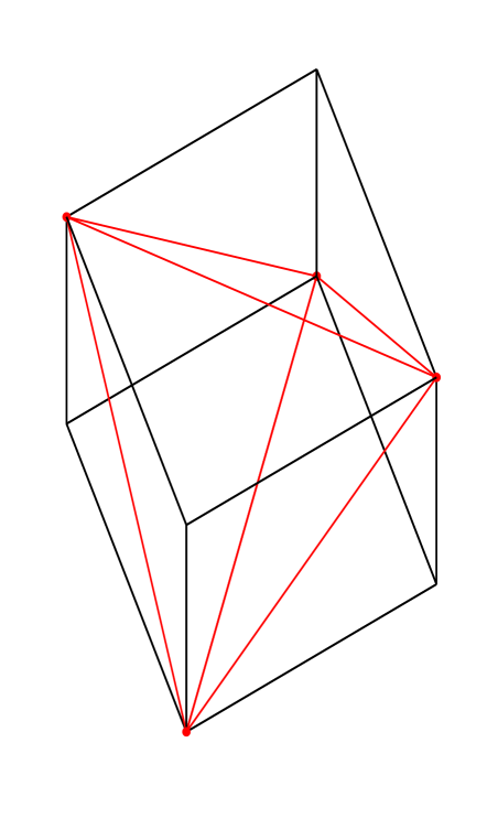
Example . For d = 3 , 𝑑 3 d=3,
H d + 1 = H 4 = [ 1 1 1 1 1 − 1 1 − 1 1 1 − 1 − 1 1 − 1 − 1 1 ] subscript 𝐻 𝑑 1 subscript 𝐻 4 delimited-[] 1 1 1 1 1 1 1 1 1 1 1 1 1 1 1 1 H_{d+1}=H_{4}=\left[\begin{array}[]{rrrr}1&1&1&1\cr 1&-1&1&-1\cr 1&1&-1&-1\cr 1&-1&-1&1\cr\end{array}\right]
so that the four points are
( 1 , 1 , 1 ) , ( − 1 , 1 , − 1 ) , ( 1 , − 1 , − 1 ) , ( − 1 , − 1 , 1 ) . 1 1 1 1 1 1 1 1 1 1 1 1
(1,1,1),\,(-1,1,-1),\,(1,-1,-1),\,(-1,-1,1).
The simplex with these vertices is shown in Figure 1 below.
Figure 1: Regular Simplex Inscribed in the Cube
The associated fundamental Lagrange polynomials are
[ ℓ 1 ( 𝐱 ) , ⋯ , ℓ d + 1 ( 𝐱 ) ] = [ 1 , 𝐱 t ] V d − 1 = 1 d + 1 [ 1 , 𝐱 t ] V d t . subscript ℓ 1 𝐱 ⋯ subscript ℓ 𝑑 1 𝐱
1 superscript 𝐱 𝑡 superscript subscript 𝑉 𝑑 1 1 𝑑 1 1 superscript 𝐱 𝑡 superscript subscript 𝑉 𝑑 𝑡 [\ell_{1}({\bf x}),\cdots,\ell_{d+1}({\bf x})]=[1,{\bf x}^{t}]V_{d}^{-1}=\frac{1}{d+1}[1,{\bf x}^{t}]V_{d}^{t}.
They have the property that
∑ i = 1 d + 1 ℓ i 2 ( 𝐱 ) superscript subscript 𝑖 1 𝑑 1 superscript subscript ℓ 𝑖 2 𝐱 \displaystyle\sum_{i=1}^{d+1}\ell_{i}^{2}({\bf x}) = \displaystyle= [ ℓ 1 ( 𝐱 ) , ⋯ , ℓ d + 1 ( 𝐱 ) ] × [ ℓ 1 ( 𝐱 ) ⋅ ⋅ ℓ d + 1 ( 𝐱 ) ] subscript ℓ 1 𝐱 ⋯ subscript ℓ 𝑑 1 𝐱
delimited-[] subscript ℓ 1 𝐱 ⋅ ⋅ subscript ℓ 𝑑 1 𝐱 \displaystyle[\ell_{1}({\bf x}),\cdots,\ell_{d+1}({\bf x})]\times\left[\begin{array}[]{c}\ell_{1}({\bf x})\cr\cdot\cr\cdot\cr\ell_{d+1}({\bf x})\end{array}\right]
= \displaystyle= 1 ( d + 1 ) 2 [ 1 , 𝐱 t ] V d t V d [ 1 𝐱 ] 1 superscript 𝑑 1 2 1 superscript 𝐱 𝑡 superscript subscript 𝑉 𝑑 𝑡 subscript 𝑉 𝑑 delimited-[] 1 𝐱 \displaystyle\frac{1}{(d+1)^{2}}[1,{\bf x}^{t}]V_{d}^{t}V_{d}\left[\begin{array}[]{c}1\cr{\bf x}\end{array}\right]
= \displaystyle= 1 + ‖ 𝐱 ‖ 2 2 d + 1 ≤ 1 1 superscript subscript norm 𝐱 2 2 𝑑 1 1 \displaystyle\frac{1+\|{\bf x}\|_{2}^{2}}{d+1}\leq 1
for all x ¯ ∈ [ − 1 , 1 ] d . ¯ x superscript 1 1 𝑑 {\b{x}}\in[-1,1]^{d}.
In other words, they are also a set of Féjer points. We mention again that, as shown in [2 ] , this is also sufficient to prove that the points X d subscript 𝑋 𝑑 X_{d}
Remark . Such points X d subscript 𝑋 𝑑 X_{d} regular simplex. As the Vandermonde determinant is a (dimensional) multiple of the volume of this simplex, it is of maximal volume. Also, as the sum of the Lagrange polynomials squared is bounded by 1 on the circumball B d := 𝐱 ∈ ℝ d : ‖ 𝐱 ‖ 2 ≤ d , : assign subscript 𝐵 𝑑 𝐱 superscript ℝ 𝑑 subscript norm 𝐱 2 𝑑 B_{d}:={{\bf x}\in\mathbb{R}^{d}\,:\,\|{\bf x}\|_{2}\leq\sqrt{d}}, X d subscript 𝑋 𝑑 X_{d} B d . subscript 𝐵 𝑑 B_{d}. □ □ \square
In particular, we have again that
Λ 1 ≤ d + 1 . subscript Λ 1 𝑑 1 \Lambda_{1}\leq\sqrt{d+1}.
We claim that in certain dimensions this upper bound is also attained.
Proposition 3.2 .
In case d = m 2 − 1 𝑑 superscript 𝑚 2 1 d=m^{2}-1 H m subscript 𝐻 𝑚 H_{m} H d + 1 = H m ⊗ H m subscript 𝐻 𝑑 1 tensor-product subscript 𝐻 𝑚 subscript 𝐻 𝑚 H_{d+1}=H_{m}\otimes H_{m}
Λ 1 = d + 1 . subscript Λ 1 𝑑 1 \Lambda_{1}=\sqrt{d+1}.
Proof . We have
Λ 1 subscript Λ 1 \displaystyle\Lambda_{1} = max 𝐱 ∈ [ − 1 , 1 ] d ∑ j = 1 d + 1 | ℓ j ( 𝐱 ) | absent subscript 𝐱 superscript 1 1 𝑑 superscript subscript 𝑗 1 𝑑 1 subscript ℓ 𝑗 𝐱 \displaystyle=\max_{{\bf x}\in[-1,1]^{d}}\sum_{j=1}^{d+1}|\ell_{j}({\bf x})|
= max 𝐱 ∈ { ± 1 } d ∑ j = 1 d + 1 | ℓ j ( 𝐱 ) | absent subscript 𝐱 superscript plus-or-minus 1 𝑑 superscript subscript 𝑗 1 𝑑 1 subscript ℓ 𝑗 𝐱 \displaystyle=\max_{{\bf x}\in\{\pm 1\}^{d}}\sum_{j=1}^{d+1}|\ell_{j}({\bf x})|
= max 𝐱 ∈ { ± 1 } d max ϵ ∈ { ± 1 } d + 1 ∑ j = 1 d + 1 ϵ j ℓ j ( 𝐱 ) absent subscript 𝐱 superscript plus-or-minus 1 𝑑 subscript bold-italic-ϵ superscript plus-or-minus 1 𝑑 1 superscript subscript 𝑗 1 𝑑 1 subscript italic-ϵ 𝑗 subscript ℓ 𝑗 𝐱 \displaystyle=\max_{{\bf x}\in\{\pm 1\}^{d}}\max_{{\bm{\epsilon}}\in\{\pm 1\}^{d+1}}\sum_{j=1}^{d+1}\epsilon_{j}\ell_{j}({\bf x})
= max 𝐱 ∈ { ± 1 } d max ϵ ∈ { ± 1 } d + 1 1 d + 1 [ 1 𝐱 t ] H d + 1 t ϵ . absent subscript 𝐱 superscript plus-or-minus 1 𝑑 subscript bold-italic-ϵ superscript plus-or-minus 1 𝑑 1 1 𝑑 1 delimited-[] 1 superscript 𝐱 𝑡 superscript subscript 𝐻 𝑑 1 𝑡 bold-italic-ϵ \displaystyle=\max_{{\bf x}\in\{\pm 1\}^{d}}\max_{{\bm{\epsilon}}\in\{\pm 1\}^{d+1}}\frac{1}{d+1}[1\,\,{\bf x}^{t}]H_{d+1}^{t}{\bm{\epsilon}}.
Hence it suffices to exhibit 𝐱 ∈ { ± 1 } d , 𝐱 superscript plus-or-minus 1 𝑑 {\bf x}\in\{\pm 1\}^{d}, ϵ ∈ { ± 1 } d + 1 bold-italic-ϵ superscript plus-or-minus 1 𝑑 1 {\bm{\epsilon}}\in\{\pm 1\}^{d+1}
1 d + 1 [ 1 𝐱 t ] H d + 1 t ϵ = d + 1 . 1 𝑑 1 delimited-[] 1 superscript 𝐱 𝑡 superscript subscript 𝐻 𝑑 1 𝑡 bold-italic-ϵ 𝑑 1 \frac{1}{d+1}[1\,\,{\bf x}^{t}]H_{d+1}^{t}{\bm{\epsilon}}=\sqrt{d+1}.
Now write, in columns,
H m = [ 𝐡 1 𝐡 2 , ⋯ , 𝐡 m ] , subscript 𝐻 𝑚 subscript 𝐡 1 subscript 𝐡 2 ⋯ subscript 𝐡 𝑚
H_{m}=[{\bf h}_{1}\,\,{\bf h}_{2},\cdots,{\bf h}_{m}],
with 𝐡 j ∈ ℝ m , subscript 𝐡 𝑗 superscript ℝ 𝑚 {\bf h}_{j}\in\mathbb{R}^{m},
ϵ = [ 𝐡 1 𝐡 2 ⋅ ⋅ 𝐡 m ] ∈ ℝ m 2 . bold-italic-ϵ delimited-[] subscript 𝐡 1 subscript 𝐡 2 ⋅ ⋅ subscript 𝐡 𝑚 superscript ℝ superscript 𝑚 2 {\bm{\epsilon}}=\left[\begin{array}[]{c}{\bf h}_{1}\cr{\bf h}_{2}\cr\cdot\cr\cdot\cr{\bf h}_{m}\end{array}\right]\in\mathbb{R}^{m^{2}}.
Note that H m t H m = m I m superscript subscript 𝐻 𝑚 𝑡 subscript 𝐻 𝑚 𝑚 subscript 𝐼 𝑚 H_{m}^{t}H_{m}=mI_{m}
H m t 𝐡 j = m 𝐞 j superscript subscript 𝐻 𝑚 𝑡 subscript 𝐡 𝑗 𝑚 subscript 𝐞 𝑗 H_{m}^{t}{\bf h}_{j}=m{\bf e}_{j}
the canonical basis vector.
Further, as H d + 1 = H m 2 = H m ⊗ H m , subscript 𝐻 𝑑 1 subscript 𝐻 superscript 𝑚 2 tensor-product subscript 𝐻 𝑚 subscript 𝐻 𝑚 H_{d+1}=H_{m^{2}}=H_{m}\otimes H_{m},
H d + 1 t = [ H i j ] 1 ≤ i , j ≤ m , H i j = ± H m t . formulae-sequence superscript subscript 𝐻 𝑑 1 𝑡 subscript delimited-[] subscript 𝐻 𝑖 𝑗 formulae-sequence 1 𝑖 𝑗 𝑚 subscript 𝐻 𝑖 𝑗 plus-or-minus superscript subscript 𝐻 𝑚 𝑡 H_{d+1}^{t}=[H_{ij}]_{1\leq i,j\leq m},\,\,\,H_{ij}=\pm H_{m}^{t}.
It follows that the i 𝑖 i H d + 1 t ϵ superscript subscript 𝐻 𝑑 1 𝑡 bold-italic-ϵ H_{d+1}^{t}{\bm{\epsilon}}
( H d + 1 t ϵ ) i subscript superscript subscript 𝐻 𝑑 1 𝑡 bold-italic-ϵ 𝑖 \displaystyle(H_{d+1}^{t}{\bm{\epsilon}})_{i} = ∑ j = 1 m ( ± 1 ) H m 𝐡 j t absent superscript subscript 𝑗 1 𝑚 plus-or-minus 1 subscript 𝐻 𝑚 superscript subscript 𝐡 𝑗 𝑡 \displaystyle=\sum_{j=1}^{m}(\pm 1)H_{m}{{}^{t}\bf h}_{j}
= ∑ j = 1 m ( ± m ) 𝐞 j absent superscript subscript 𝑗 1 𝑚 plus-or-minus 𝑚 subscript 𝐞 𝑗 \displaystyle=\sum_{j=1}^{m}(\pm m){\bf e}_{j}
which is a vector all of whose components are ± m . plus-or-minus 𝑚 \pm m. H d + 1 t ϵ ∈ ℝ m 2 superscript subscript 𝐻 𝑑 1 𝑡 bold-italic-ϵ superscript ℝ superscript 𝑚 2 H_{d+1}^{t}{\bm{\epsilon}}\in\mathbb{R}^{m^{2}} ± m . plus-or-minus 𝑚 \pm m. + 1 . 1 +1.
x j := sgn ( H d + 1 ϵ ) j + 1 assign subscript 𝑥 𝑗 sgn subscript subscript 𝐻 𝑑 1 bold-italic-ϵ 𝑗 1 x_{j}:={\rm sgn}(H_{d+1}{\bm{\epsilon}})_{j+1}
we obtain
1 d + 1 [ 1 𝐱 t ] H d + 1 t ϵ 1 𝑑 1 delimited-[] 1 superscript 𝐱 𝑡 superscript subscript 𝐻 𝑑 1 𝑡 bold-italic-ϵ \displaystyle\frac{1}{d+1}[1\,\,{\bf x}^{t}]H_{d+1}^{t}{\bm{\epsilon}} = 1 d + 1 ‖ H d + 1 t ϵ ‖ 1 absent 1 𝑑 1 subscript norm superscript subscript 𝐻 𝑑 1 𝑡 bold-italic-ϵ 1 \displaystyle=\frac{1}{d+1}\|H_{d+1}^{t}{\bm{\epsilon}}\|_{1}
= 1 d + 1 ( d + 1 ) m absent 1 𝑑 1 𝑑 1 𝑚 \displaystyle=\frac{1}{d+1}(d+1)m
= m = d + 1 . absent 𝑚 𝑑 1 \displaystyle=m=\sqrt{d+1}.
□ □ \square
4 K 𝐾 K
There are analogous results for the complex version of the cube, the Torus. Consider
K = 𝕋 d := { 𝐳 ∈ ℂ d : | z j | = 1 , 1 ≤ j ≤ d } . 𝐾 superscript 𝕋 𝑑 assign conditional-set 𝐳 superscript ℂ 𝑑 formulae-sequence subscript 𝑧 𝑗 1 1 𝑗 𝑑 K=\mathbb{T}^{d}:=\{{\bf z}\in\mathbb{C}^{d}\,:\,|z_{j}|=1,\,\,1\leq j\leq d\}.
In this case the classical Fourier matrix plays the role of the Hadamard matrix.
Definition 4.1 .
The Fourier matrix F n ∈ ℂ n × n subscript 𝐹 𝑛 superscript ℂ 𝑛 𝑛 F_{n}\in\mathbb{C}^{n\times n}
F n := [ ω j k ] 1 ≤ j , k ≤ n , ω := exp ( 2 π i / n ) formulae-sequence assign subscript 𝐹 𝑛 subscript delimited-[] superscript 𝜔 𝑗 𝑘 formulae-sequence 1 𝑗 𝑘 𝑛 assign 𝜔 2 𝜋 𝑖 𝑛 F_{n}:=[\omega^{jk}]_{1\leq j,k\leq n},\quad\omega:=\exp(2\pi i/n)
is known as the Fourier matrix.
As is well known, the Fourier matrix has orthogonal rows and columns, i.e.,
F n ∗ F n = n I n superscript subscript 𝐹 𝑛 subscript 𝐹 𝑛 𝑛 subscript 𝐼 𝑛 F_{n}^{*}F_{n}=nI_{n}
and is sometimes referred to as a complex Hadamard matrix, as the entries all have modulus 1 . 1 1.
Just as for the cube and Hadamard matrix we let
X d ∈ ℂ ( d + 1 ) × d subscript 𝑋 𝑑 superscript ℂ 𝑑 1 𝑑 X_{d}\in\mathbb{C}^{(d+1)\times d} F d + 1 . subscript 𝐹 𝑑 1 F_{d+1}. d + 1 𝑑 1 d+1 X d subscript 𝑋 𝑑 X_{d} d + 1 𝑑 1 d+1 𝕋 d . superscript 𝕋 𝑑 \mathbb{T}^{d}. V d := F d + 1 assign subscript 𝑉 𝑑 subscript 𝐹 𝑑 1 V_{d}:=F_{d+1}
{ 1 , z 1 , ⋯ , z d } . 1 subscript 𝑧 1 ⋯ subscript 𝑧 𝑑 \{1,z_{1},\cdots,z_{d}\}.
The associated fundamental Lagrange polynomials are
[ ℓ 1 ( 𝐳 ) ⋅ ⋅ ℓ d + 1 ( 𝐳 ) ] delimited-[] subscript ℓ 1 𝐳 ⋅ ⋅ subscript ℓ 𝑑 1 𝐳 \displaystyle\left[\begin{array}[]{c}\ell_{1}({\bf z})\cr\cdot\cr\cdot\cr\ell_{d+1}({\bf z})\end{array}\right] = V d − t [ 1 𝐳 ] absent superscript subscript 𝑉 𝑑 𝑡 delimited-[] 1 𝐳 \displaystyle=V_{d}^{-t}\left[\begin{array}[]{c}1\cr{\bf z}\end{array}\right]
= V d − 1 [ 1 𝐳 ] ( as F n t = F n ) absent superscript subscript 𝑉 𝑑 1 delimited-[] 1 𝐳 as superscript subscript 𝐹 𝑛 𝑡 subscript 𝐹 𝑛
\displaystyle=V_{d}^{-1}\left[\begin{array}[]{c}1\cr{\bf z}\end{array}\right]\quad({\rm as}\,\,F_{n}^{t}=F_{n})
= 1 d + 1 V d ∗ [ 1 𝐳 ] . absent 1 𝑑 1 superscript subscript 𝑉 𝑑 delimited-[] 1 𝐳 \displaystyle=\frac{1}{d+1}V_{d}^{*}\left[\begin{array}[]{c}1\cr{\bf z}\end{array}\right].
They have the property that
∑ i = 1 d + 1 | ℓ i ( 𝐳 ) | 2 superscript subscript 𝑖 1 𝑑 1 superscript subscript ℓ 𝑖 𝐳 2 \displaystyle\sum_{i=1}^{d+1}|\ell_{i}({\bf z})|^{2} = \displaystyle= [ ℓ 1 ( 𝐳 ) ⋅ ⋅ ℓ d + 1 ( 𝐳 ) ] ∗ × [ ℓ 1 ( 𝐳 ) ⋅ ⋅ ℓ d + 1 ( 𝐳 ) ] superscript delimited-[] subscript ℓ 1 𝐳 ⋅ ⋅ subscript ℓ 𝑑 1 𝐳 delimited-[] subscript ℓ 1 𝐳 ⋅ ⋅ subscript ℓ 𝑑 1 𝐳 \displaystyle\left[\begin{array}[]{c}\ell_{1}({\bf z})\cr\cdot\cr\cdot\cr\ell_{d+1}({\bf z})\end{array}\right]^{*}\times\left[\begin{array}[]{c}\ell_{1}({\bf z})\cr\cdot\cr\cdot\cr\ell_{d+1}({\bf z})\end{array}\right]
= \displaystyle= 1 ( d + 1 ) 2 [ 1 , 𝐳 ∗ ] V d V d ∗ [ 1 𝐳 ] 1 superscript 𝑑 1 2 1 superscript 𝐳 subscript 𝑉 𝑑 superscript subscript 𝑉 𝑑 delimited-[] 1 𝐳 \displaystyle\frac{1}{(d+1)^{2}}[1,{\bf z}^{*}]V_{d}V_{d}^{*}\left[\begin{array}[]{c}1\cr{\bf z}\end{array}\right]
= \displaystyle= 1 + ‖ 𝐳 ‖ 2 2 d + 1 ≤ 1 1 superscript subscript norm 𝐳 2 2 𝑑 1 1 \displaystyle\frac{1+\|{\bf z}\|_{2}^{2}}{d+1}\leq 1
for all 𝐳 ∈ 𝕋 d . 𝐳 superscript 𝕋 𝑑 {\bf z}\in\mathbb{T}^{d}.
In other words, they are also a set of Féjer points. and this is sufficient to show that the points X d subscript 𝑋 𝑑 X_{d}
Proposition 4.2 .
For K = 𝕋 d , 𝐾 superscript 𝕋 𝑑 K=\mathbb{T}^{d}, d = m 2 − 1 𝑑 superscript 𝑚 2 1 d=m^{2}-1 m , 𝑚 m,
Λ 1 = d + 1 . subscript Λ 1 𝑑 1 \Lambda_{1}=\sqrt{d+1}.
Proof . From the fact that X d subscript 𝑋 𝑑 X_{d}
Λ 1 ≤ d + 1 . subscript Λ 1 𝑑 1 \Lambda_{1}\leq\sqrt{d+1}.
To show the lower bound we argue as for the real cube with H d + 1 subscript 𝐻 𝑑 1 H_{d+1} F d + 1 , subscript 𝐹 𝑑 1 F_{d+1}, d + 1 = m 2 , 𝑑 1 superscript 𝑚 2 d+1=m^{2}, F d + 1 = F m ⊗ F m . subscript 𝐹 𝑑 1 tensor-product subscript 𝐹 𝑚 subscript 𝐹 𝑚 F_{d+1}=F_{m}\otimes F_{m}.
Λ 1 subscript Λ 1 \displaystyle\Lambda_{1} = max 𝐳 ∈ 𝕋 d ∑ j = 1 d + 1 | ℓ j ( 𝐳 ) | absent subscript 𝐳 superscript 𝕋 𝑑 superscript subscript 𝑗 1 𝑑 1 subscript ℓ 𝑗 𝐳 \displaystyle=\max_{{\bf z}\in\mathbb{T}^{d}}\sum_{j=1}^{d+1}|\ell_{j}({\bf z})|
= max 𝐳 ∈ 𝕋 d max | ϵ j | ≤ 1 , 1 ≤ j ≤ ( d + 1 ) ∑ j = 1 d + 1 ϵ j ℓ j ( 𝐳 ) ¯ absent subscript 𝐳 superscript 𝕋 𝑑 subscript formulae-sequence subscript italic-ϵ 𝑗 1 1 𝑗 𝑑 1 superscript subscript 𝑗 1 𝑑 1 subscript italic-ϵ 𝑗 ¯ subscript ℓ 𝑗 𝐳 \displaystyle=\max_{{\bf z}\in\mathbb{T}^{d}}\max_{|\epsilon_{j}|\leq 1,\,1\leq j\leq(d+1)}\sum_{j=1}^{d+1}\epsilon_{j}\overline{\ell_{j}({\bf z})}
= max 𝐳 ∈ 𝕋 d max | ϵ j | ≤ 1 , 1 ≤ j ≤ ( d + 1 ) 1 d + 1 [ 1 𝐳 ∗ ] F d + 1 ϵ . absent subscript 𝐳 superscript 𝕋 𝑑 subscript formulae-sequence subscript italic-ϵ 𝑗 1 1 𝑗 𝑑 1 1 𝑑 1 delimited-[] 1 superscript 𝐳 subscript 𝐹 𝑑 1 bold-italic-ϵ \displaystyle=\max_{{\bf z}\in\mathbb{T}^{d}}\max_{|\epsilon_{j}|\leq 1,\,1\leq j\leq(d+1)}\frac{1}{d+1}[1\,\,{\bf z}^{*}]F_{d+1}{\bm{\epsilon}}.
Hence it suffices to exhibit 𝐳 ∈ 𝕋 d 𝐳 superscript 𝕋 𝑑 {\bf z}\in\mathbb{T}^{d} ϵ ∈ ℂ d + 1 bold-italic-ϵ superscript ℂ 𝑑 1 {\bm{\epsilon}}\in\mathbb{C}^{d+1} | ϵ j | ≤ 1 , subscript italic-ϵ 𝑗 1 |\epsilon_{j}|\leq 1, 1 ≤ j ≤ d + 1 , 1 𝑗 𝑑 1 1\leq j\leq d+1,
1 d + 1 [ 1 𝐳 t ] F d + 1 ϵ = d + 1 . 1 𝑑 1 delimited-[] 1 superscript 𝐳 𝑡 subscript 𝐹 𝑑 1 bold-italic-ϵ 𝑑 1 \frac{1}{d+1}[1\,\,{\bf z}^{t}]F_{d+1}{\bm{\epsilon}}=\sqrt{d+1}.
It is easy to verify that ϵ bold-italic-ϵ {\bm{\epsilon}} F m ∗ superscript subscript 𝐹 𝑚 F_{m}^{*} 𝐳 𝐳 {\bf z} □ □ \square