DeepAqua: Self-Supervised Semantic Segmentation of Wetland Surface Water Extent with SAR Images using Knowledge Distillation

Abstract

Deep learning and remote sensing techniques have significantly advanced water monitoring abilities; however, the need for annotated data remains a challenge. This is particularly problematic in wetland detection, where water extent varies over time and space, demanding multiple annotations for the same area. In this paper, we present DeepAqua, a self-supervised deep learning model that leverages knowledge distillation (a.k.a. teacher-student model) to eliminate the need for manual annotations during the training phase. We utilize the Normalized Difference Water Index (NDWI)as a teacher model to train a Convolutional Neural Network (CNN)for segmenting water from Synthetic Aperture Radar (SAR)images, and to train the student model, we exploit cases where optical- and radar-based water masks coincide, enabling the detection of both open and vegetated water surfaces. DeepAqua represents a significant advancement in computer vision techniques by effectively training semantic segmentation models without any manually annotated data. Experimental results show that DeepAqua outperforms other unsupervised methods by improving accuracy by 7%, Intersection Over Union by 27%, and F1 score by 14%. This approach offers a practical solution for monitoring wetland water extent changes without needing ground truth data, making it highly adaptable and scalable for wetland conservation efforts.

[su]organization=Department of Physical Geography, Stockholm University,addressline=Svante Arrhenius väg 8, city=Stockholm, postcode=106 91, country=Sweden

[kth]organization=Division of Software and Computer Systems, KTH Royal Institute of Technology,addressline=Kistagången 16, city=Kista, postcode=164 40, country=Sweden

1 Introduction

Wetlands provide essential ecosystem services such as water purification, flood regulation, and carbon sequestration, and are critical for sustainable development (Jaramillo et al., 2019). They are, however, increasingly threatened by climate change and human activity (Thorslund et al., 2017). The comprehensive monitoring of wetland surface water extent, including both open and vegetated water surfaces, is essential for the effective wetland monitoring needed for their conservation and management.

Advancements in remote sensing techniques have greatly improved surface water monitoring capabilities (Feyisa et al., 2014). While optical sensors are adept at detecting open water surfaces, they struggle to identify vegetated waters, underestimating wetland water extent. Radar sensors, such as Synthetic Aperture Radar (SAR), can overcome this limitation by penetrating the vegetation (Banks et al., 2019). Still, analyzing SAR images can be challenging due to noise and speckles, making it difficult to distinguish water from soil and vegetation.

In recent years, deep learning techniques for the semantic segmentation of images have shown promise in addressing these challenges. However, the substantial amount of annotated data required for training these models is often time-consuming and costly, creating significant barriers to their widespread adoption. Furthermore, existing methods struggle to accurately identify vegetated waters, underestimating wetland surface water extent.

In this paper, we present DeepAqua, a self-supervised deep learning model that employs knowledge distillation (a.k.a teacher-student model) to eliminate the need for manual annotation during the training phase. Utilizing the Normalized Difference Water Index (NDWI) (McFeeters, 1996) as the “teacher” model, we train a “student” U-Net (Ronneberger et al., 2015) to recognize water boundaries in any SAR image. Using the signal from non-vegetated water as a guide, the student model learns from the teacher model, eventually recognizing both open and vegetated water bodies. The NDWI “teacher” model can generate annotated images of water surfaces without training. Here, we address the problem of how to train a deep learning model to recognize surface water from radar imagery. We aim to eliminate the costs of collecting training data through fieldwork or manual annotations of radar images.

The contributions of our paper are as follows:

• We present DeepAqua, a novel method for training semantic segmentation models using knowledge distillation without any manually annotated data.

• Our method employs NDWI masks as proxies for semantic labels and optical images as an auxiliary modality to supervise a SAR-based U-Net.

• We present DeepAqua as a highly adaptable and scalable model, as it does not require ground truth for training.

• We enhance the efficiency of wetland conservation strategies, as DeepAqua can monitor changes in surface water coverage, encompassing both exposed and vegetated aquatic areas.

2 Related Work

The challenge of accurately detecting wetlands — a critical task for environmental and societal applications such as flood mapping and water resource management — is intensified by variable spectral signatures of water resulting from illumination, turbidity, and vegetation. Multispectral optical imagery from satellites such as Sentinel-2 has been widely used to map wetlands using deep learning methods (Jiang et al., 2019; Cui et al., 2020; Dang et al., 2020; Jamali et al., 2021b; Pham et al., 2022; Onojeghuo and Onojeghuo, 2023). For example, (Rezaee et al., 2018) fine-tunes an AlexNet (Krizhevsky et al., 2017) pre-trained on the ImageNet (Deng et al., 2009) dataset to classify wetland patches using optical imagery. Mahdianpari et al. (2018) explores multiple Convolutional Neural Network (CNN) architectures to determine which architecture produced the most accurate wetland classifications. However, these approaches cannot detect water hidden under vegetation, which is crucial for monitoring water extent in wetlands.

Radar imagery from satellites such as Sentinel-1, which has a SAR C-band sensor that can penetrate vegetation and clouds (Geudtner et al., 2014), have additionally been used for this purpose. Slagter et al. (2020) combined Sentinel-1 with optical Sentinel-2 and fieldwork data to map wetlands using a random forest classifier. The WetNet model (Hosseiny et al., 2021) is an ensemble of three classifiers that uses multitemporal images to map wetlands: a 2D-CNN trained on radar imagery, a 3D-CNN trained on multispectral and multitemporal imagery, and a Recurrent Neural Network (RNN) trained with multivariate temporal information. Jamali et al. (2022) introduces the 3DUnetGSFormer model, which uses a Generative Adversarial Network (GAN) (Goodfellow et al., 2020) to generate synthetic data with similar characteristics as the ground-truth data and a Swin transformer (Liu et al., 2021) to classify the wetland images. Similar approaches have used optical and radar imagery to map wetlands, such as Jamali et al. (2021a) and Jamali and Mahdianpari (2022).

All these approaches have a common limitation: they require manually annotated data to train their models. The manually annotated data usually come from fieldwork, which is very costly and time-consuming to acquire due to logistics, equipment maintenance, sampling, etc. Moreover, these approaches assume that the surface water extent is constant over time, although the water extent usually varies across the season and is subject to weather conditions. For instance, one wetland location could have been labeled “open water” because the image was taken in April when the surface water extent of the wetland increased due to snowmelt. On the other hand, the same location could be dry in July, leading to inaccurate predictions and quantification of water surfaces.

3 Background and Problem Formulation

This paper addresses the problem of detecting water surfaces under vegetation without requiring fieldwork or manually annotated data. To create a model and train it without fieldwork or manually annotated data, we combine remote sensing techniques (Section 3.1) with deep learning techniques (Sections 3.2, 3.3, and 3.4). Here, we recall some of their basic concepts.

3.1 Detecting Surface Water using Remote Sensing

Traditionally, optical sensors based on reflected solar radiation have been used to detect water. NDWI is one of the most popular optical methods to delineate open waters (McFeeters, 1996), as it helps differentiate open water from soil since: (1) water reflects green light, (2) water has low reflectance of Near-Infrared (NIR) light, and (3) terrestrial vegetation and soil have a high reflectance of NIR light. For each pixel in an image, the NDWI is calculated using the normalized difference between the green light intensity and the NIR light intensity – the results of the NDWI index range from -1 to +1. Water surfaces have positive values, while soil and terrestrial vegetation have zero or negative values because they typically have a higher reflectance of NIR than green light. Figure 1 shows how NDWI is used to delineate open water.

Other index-based methods to detect water from optical imagery include the Modified NDWI (MNDWI) (Xu, 2006), High Resolution Water Index (HRWI) (Yao et al., 2015), Two-step Urban Water Index (TSUWI) (Wu et al., 2018) and Automated Water Extraction Index (AWEI) (Feyisa et al., 2014).

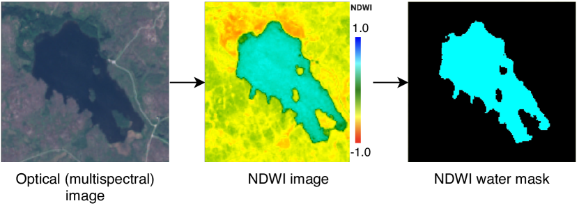
Figure 1: Water delineation using NDWI. The left image comprises red, green, and blue bands (RGB). The middle image is generated using the NDWI index. The right image shows an NDWI image where pixels with positive values are cyan, and the rest are black, thus completing the water delineation process.

Although NDWI provides reliable information on open water, its usage is limited to cloud-free days. Areas with low albedo and shadows can introduce inaccuracies in detection (Feyisa et al., 2014). On the other hand, SAR does not depend on sunlight and is able to penetrate vegetation, presenting an attractive alternative to optical imagery (Mondini et al., 2021). As such, SAR can provide data on water hidden under vegetation. However, SAR sensors provide complex information that can be challenging to interpret. Moreover, water may be mistaken with unvegetated or sparsely vegetated areas, adding additional difficulties to the automatic detection of water in SAR images (Tsyganskaya et al., 2018; Hardy et al., 2019).

3.2 Semantic Segmentation of Images

Semantic segmentation is a computer vision technique to identify and classify objects within an image at the pixel level. Instead of just identifying objects as a whole, semantic segmentation identifies the exact boundaries of each object and assigns a specific label or class to each pixel within the object’s boundary. This allows for a more precise and detailed analysis of an image, making it useful for applications such as self-driving cars, medical imaging, and, in our case, water delineation.

CNNs are one of the most efficient deep learning approaches for image processing (LeCun et al., 2015). They work by reading an image through a series of layers that extract features such as edges and shapes and then using those features to recognize patterns in the image. They extract a varying level of abstraction from the data in different layers with the added benefit of not requiring prior feature extraction and having more generalization capability. CNNs use convolutional layers to extract features, pooling layers to downsample the output, and activation functions to introduce non-linearity. CNNs have proven effective in image recognition tasks because they can learn to recognize patterns and features in images without being explicitly programmed. CNNs have better prediction accuracy because they (1) can retain the geometrical properties from two-dimensional images, (2) can be trained with large amounts of data and perform consistently across varied data, and (3) do not require expert input of features; the CNNs can learn the features.

We use a particular CNN architecture called U-Net (Ronneberger et al., 2015) for producing semantic segmentations. U-Net is designed in a way that it has a contracting path followed by an expanding path. The contracting path consists of a series of convolutional layers, reducing the spatial dimensions of the image while increasing the number of channels. This helps to extract high-level features from the input image. The expanding path then consists of a series of up-convolutional layers, which upsample the feature maps to restore the original spatial dimensions of the image, generating a segmentation map with the same dimensions as the input image. Other architectures for semantic segmentation include Resnet (He et al., 2016), MSResNet (Dang and Li, 2021), and MSCENet (Kang et al., 2021).

Here, we use knowledge distillation to train a U-Net without requiring manually annotated data.

3.3 Knowledge Distillation

Knowledge distillation (Hinton et al., 2015; Xu et al., 2020), which is also known as the teacher-student model, is a process of teaching a smaller and simpler model - the student model - to mimic the behavior of a larger and more complex model - the teacher model - to achieve similar performance. During the distillation process, the teacher model generates predictions for training data, which are then used to train the student model. However, instead of training the student model to directly predict the correct output, the student model is trained to learn from the teacher model’s predictions.

By doing so, the student model can learn from the teacher model, including the relationships between different input features and the patterns in the data, which is difficult to learn from the training data alone. The result is a smaller and faster model that performs similarly to the larger and more complex teacher model. Additionally, the student model may generalize better than the teacher model in specific scenarios (Deng et al., 2022; Beyer et al., 2022), as it has learned to capture the most important aspects of the teacher’s behavior while ignoring the noise. In this paper, we tweak the knowledge distillation process: instead of having a small model learn from a large model, we make a radar-based model learn from an optical-based model. We exploit the fact that it is easier to identify water from optical images rather than from radar images. This process is called cross-modal knowledge distillation (Hu et al., 2020). By using knowledge distillation, we create a self-supervised model.

3.4 Self-Supervised Learning

One of the biggest bottlenecks in deep learning models, including CNNs, is requiring large amounts of annotated data to make accurate predictions. Particularly in semantic segmentation of images, manually annotating each image is costly and time-consuming, aggravated by the fact that deep learning models require thousands of images to produce accurate predictions. Techniques like transfer learning (Garcia-Garcia et al., 2018) and data augmentation (Shorten and Khoshgoftaar, 2019) have alleviated the need for large amounts of annotated data. Nevertheless, they still require a minimum amount of data. Self-supervised learning is a machine learning method that allows algorithms to learn without needing human-annotated samples (Shurrab and Duwairi, 2022).

The following section shows how we achieve self-supervision using knowledge distillation architecture. We automatically generate ground truth data using NDWI and train a SAR-based CNN to detect water. Our approach has the advantage of requiring zero manually annotated data.

4 DeepAqua Model

Semantic segmentation projects typically involve a human annotator delineating images to indicate which parts correspond to a particular object or feature, such as water surfaces in radar images. This process can be time-consuming and expensive, often making data annotation the bottleneck of deep learning projects. Figure 2(a) shows this traditional architecture with a human annotator delineating the water in radar images and a CNN trained based on these annotated images to recognize water in previously unseen images.

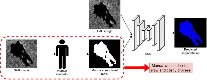
(a) The traditional methodology for training deep learning models relies on manually annotated data.

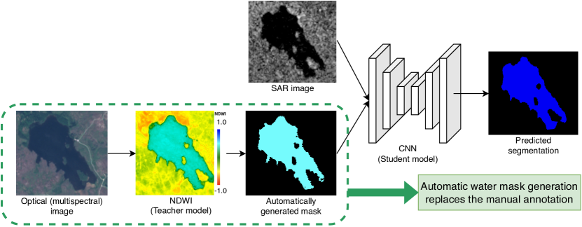
(b) Our proposed methodology automatizes the data annotation process.

Figure 2: The training of a CNN model to recognize water boundaries from SAR imagery using NDWI water masks as ground truth.

In this study, as seen in Figure 2(b), instead of relying on human-annotated water masks, our knowledge distillation architecture uses the NDWI model as the teacher and the CNN as the student, where the teacher extracts knowledge about the location of the water surface from optical imagery and produces segmented images that the student will try to mimic. Unlike most knowledge distillation approaches, our teacher and student models rely on different data types; particularly, the teacher uses optical imagery to produce water segmentations, while the student uses radar imagery. For each batch of images, we calculate the Dice loss (Soomro et al., 2018) between the student predictions and the ground truth masks provided by the teacher and minimize this loss function to improve the performance of the student model. We then backpropagate the loss to update the weights of the CNN. By eliminating the need for manual annotation, we aim to streamline the model training process and reduce overall project costs.

4.1 DeepAqua Framework and Workflow

Figure 3 shows the DeepAqua’s overall framework and workflow. Our method consists of two models: teacher and student models. The teacher model is a thresholding model that generates water masks by applying the NDWI index to optical images, and the student model which is a U-Net (Ronneberger et al., 2015) that takes SAR images as input and produces segmentation masks as output. The teacher and student models are trained jointly by minimizing the Dice loss between their outputs. The workflow of our method is as follows:

• Step 1: We create a training set by selecting images that fulfil the following conditions: (1) Sentinel-1 and Sentinel-2 image availability on the same date for the region of interest, (2) a maximum of 1% of cloud cover on the Sentinel-2 image, and (3) no missing values on the Sentinel-1 and Sentinel-2 images.

• Step 2: Given a pair of optical and SAR images that are co-registered and cover the same geographic area, we feed the optical image to the teacher model and obtain an NDWI mask as its output.

• Step 3: We feed the SAR image to the student model and obtain a segmentation mask as its output.

• Step 4: We compute the Dice loss between the teacher and student output to measure their similarity.

• Step 5: We update the student weights using backpropagation based on the Dice loss.

• Step 6: We repeat steps 2-5 for all pairs of optical and SAR images in the training set until convergence.

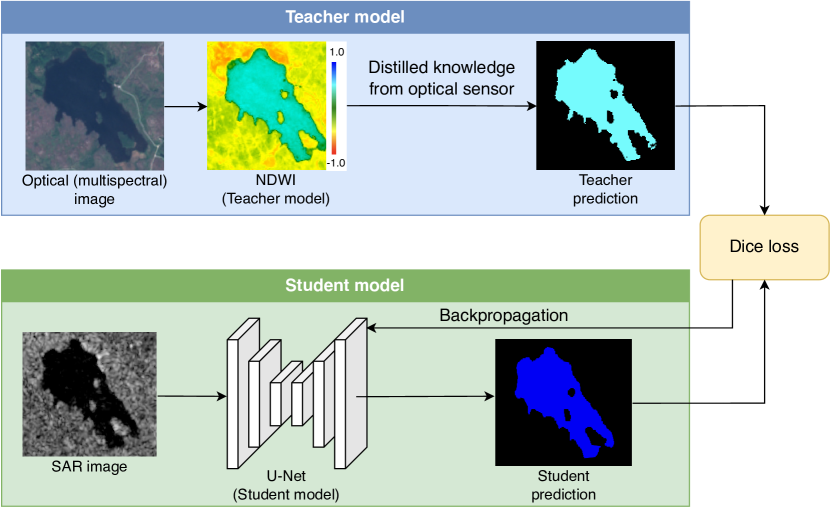
Figure 3: The process of training a CNN model to recognize water boundaries from SAR imagery by learning from a NDWI model.

4.2 The Teacher Model

The teacher model generates water masks from optical images using the NDWI index. Selecting the optimal threshold for NDWI values is challenging, as highlighted by Ji et al. (2009) and Reis et al. (2021). Following the recommendation of McFeeters (1996), we adopted a threshold value of 0.0 to delineate open water. The teacher model outputs a binary water mask matching the input optical image size, where 0 indicates ground and 1 denotes water. This mask then guides the student model.

4.3 The Student Model

The student model is a U-Net (Ronneberger et al., 2015) model that takes SAR images as input and produces segmentation masks as output. We use U-Net as the student model for two reasons. First, U-Net is a simple and effective model for semantic segmentation that can achieve good results with limited data and computational resources. Second, U-Net is compatible with the teacher model regarding input and output sizes, facilitating the cross-modal knowledge distillation process.

We train U-Net from scratch on SAR images without requiring annotated data. We use SAR images from Sentinel-1, a satellite mission that provides C-band SAR images with a resolution of $10$m $\times 10$m per pixel. For enhanced contrast in these images, we exclude pixel values below the 1st percentile and above the 99th percentile. Subsequently, we normalize the images. The output of the U-Net is a segmentation mask that has the same size as the input SAR image. Within this mask, values span from 0 to 1, with higher values suggesting increased water presence. This segmentation mask serves as the desired output for model optimization.

4.4 The Cross-Modal Knowledge Distillation Process

The cross-modal knowledge distillation process is the core of our method that transfers knowledge from the teacher to the student model. The teacher model produces a hard NDWI water mask from an optical image, and the student model produces a segmentation mask from a SAR image. The hard NDWI mask and the segmentation mask are aligned in terms of spatial resolution and geographic area, as they are generated from co-registered optical and SAR images that cover the same scene. The cross-modal knowledge distillation process aims to minimize the Dice loss between the NDWI mask and the segmentation mask, which measures their similarity.

The Dice loss (Dice, 1945) is a loss function frequently employed for semantic segmentation tasks. It’s particularly suited for imbalanced data, where one class (e.g., water pixels) might be significantly underrepresented compared to another (e.g., land pixels). The Dice loss is defined as:

$$\mathcal{L}_{Dice}=1-\frac{2\times|Y_{T}*Y_{S}|+\epsilon}{|Y_{T}|+|Y_{S}|+\epsilon}$$ (1)

where $Y_{T}$ and $Y_{S}$ are the teacher output and the student output, respectively, $|\cdot|$ denotes the sum of all elements in a matrix, $*$ denotes element-wise multiplication, and $\epsilon$ is a small constant to avoid division by zero. The Dice loss ranges from 0 to 1, where lower values indicate higher similarity.

By minimizing the Dice loss, the student model learns to mimic the teacher model’s output and thus segment SAR images without requiring annotated data. The Dice loss provides a soft and smooth supervision signal for the student model, as it considers true positives in the numerator and true positives, false positives, and false negatives in the denominator. This Dice loss formula helps solve the issue of imbalanced training data and does not require defining weighting parameters between different classes (in our case, the ground and water). Besides, the function works well for binary segmentation tasks (Soomro et al., 2018).

4.5 The Backpropagation Algorithm

The backpropagation algorithm is the algorithm that updates the student weights based on the Dice loss. The backpropagation algorithm consists of two steps: forward and backward propagation. In the forward propagation, we compute the teacher output, the student output, and the Dice loss for a given pair of optical and SAR images. In the backward propagation, we calculate the gradient of the Dice loss with respect to the student weights and update the weights using an optimizer.

The steps of the backpropagation algorithm are as follows:

• Step 1: Given a pair of optical and SAR images ($X_{O}$, $X_{S}$), we feed $X_{O}$ to the teacher model and $X_{S}$ to the student model. We then obtain $Y_{T}$ and $Y_{S}$ as the teacher’s and student’s outputs, respectively.

• Step 2: Compute $\mathcal{L}_{Dice}$ using $Y_{T}$ and $Y_{S}$ as inputs.

• Step 3: Compute $\partial\mathcal{L}_{Dice}/\partial W_{S}$ using the chain rule, where $W_{S}$ are the student weights.

• Step 4: Update $W_{S}$ using an optimizer (e.g., Adam (Kingma and Ba, 2015)).

• Step 5: Repeat steps 1-4 for all pairs of optical and SAR images in training set until convergence.

5 Evaluation

We evaluated the performance of DeepAqua using SAR-Vertical-Horizontal (VH) imagery downloaded from Google Earth Engine (Gorelick et al., 2017).

5.1 Training, Validation, and Testing Datasets

To train DeepAqua, we used Sentinel-1 (SAR) and Sentinel-2 (multispectral) images of the entire county of Örebro in Sweden. Örebro has an area of $(\sim 8550$ km${}^{2})$. We used Sentinel-2 multispectral images and then applied NDWI to generate water masks. To this end, we first split the entire Örebro region into tiles of $64\times 64$ pixels. Each pixel had a resolution of $10$ meters. Then, we repeated the same procedure to generate a SAR dataset using Sentinel-1 images from the same region. This resulted in a total of $45\,500$ multispectral-SAR pairs. Figure 4 illustrates how we generated the data to train our model. Once we generated all the data, we randomly selected 80% of the tiles to create a training set, and we took the remaining 20% to create a validation set.

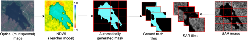
Figure 4: The process of automatically generating the training set. We create multispectral-SAR pairs by splitting the satellite images into smaller tiles.

Our testing set is composed of imagery from Svartådalen, Hjälstaviken and Hornborgasjön, three wetlands that belong to the Ramsar convention, as shown in Figure 5. The three wetlands are located in flat areas of Southern and Western Sweden. These are shallow wetlands that are not connected to any important river stream and are rather fed by small streams with low flow rates. The wetlands are convered by emerging grassy vegetation mainly consisting of mires, and open water bodies. The grassy vegetation is often flooded during the rainy season and during spring when the wetlands receive snowmelt from upstream. Some borders of the wetlands have also tree canopies that do not allow the penetration of C-band signals. However, these areas are not connected to the grassy areas and are far from the open water bodies. Svartådalen is a mixed wetland complex of $1\,977$ ha comprised of mires, bogs, and fens. Hjälstaviken is a limnic complex of $808$ ha. Hornborgasjön is a human-made mire complex of $6\,197$ ha, one of the largest single nature conservation projects ever carried out in Sweden (Gunnarsson and Löfroth, 2014; Matthews et al., 1993). We manually delineated the water in radar imagery from the study sites. Each site contains 40 images between 2018 and 2022. We excluded the months of January, February, March, and December to avoid images that contained snow.

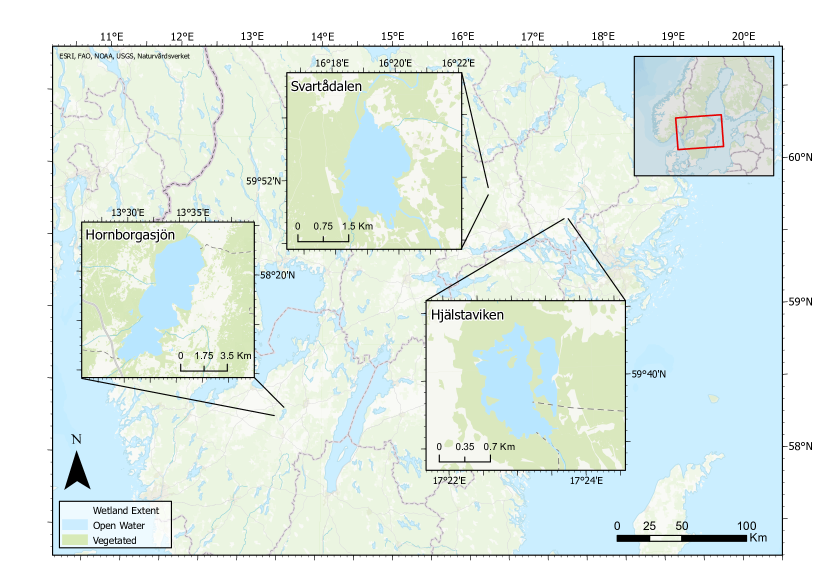
Figure 5: Map of Sweden containing the location of the three wetlands with manually annotated data that compose the testing set.

5.2 Evaluation Metrics

To quantitatively evaluate the performance of our semantic segmentation model on radar imagery of wetlands, we employed a set of evaluation metrics as detailed in (Everingham et al., 2015). These metrics, derived from True Negatives (TP), True Negatives (TN), False Positives (FP), and False Negatives (FN) counts, measure both pixel-level accuracy and the overall quality of the segmented regions.

1. Pixel Accuracy (PA): This metric computes the proportion of correctly classified pixels in the entire image. It provides an overall sense of how well the model is performing but may not capture errors distributed across different classes effectively: $\frac{\text{TP}+\text{TN}}{\text{TP}+\text{TN}+\text{FP}+\text{FN}}$.

2. Intersection Over Union (IOU): Also known as the Jaccard index, Intersection Over Union (IOU) offers a measure of the overlap between the predicted and true areas, with values ranging from 0 (no overlap) to 1 (perfect overlap): $\frac{\text{TP}}{\text{TP}+\text{FP}+\text{FN}}$

3. Precision: This quantifies the proportion of positive identifications (i.e., water pixels) that were actually correct. A high precision indicates that the model has fewer false positives: $\frac{\text{TP}}{\text{TP}+\text{FP}}$

4. Recall: Also known as sensitivity, recall measures the proportion of actual positives (water pixels in ground truth) that are identified correctly. A high recall means the model has fewer false negatives: $\frac{\text{TP}}{\text{TP}+\text{FN}}$

5. F1-Score: The harmonic mean of precision and recall, the F1-score gives a balanced measure of the model’s performance, especially when the class distribution is imbalanced: $2\times\frac{\text{Precision}\times\text{Recall}}{\text{Precision}+\text{Recall}}$

By employing these metrics, we aim to comprehensively evaluate our model’s capabilities, considering both the finer details and the broader context of water segmentation in radar imagery.

5.3 Baseline Method

We compared the performance of DeepAqua against Otsu’s method (Otsu, 1979). We selected this method because it is unsupervised, aligning with our study’s central theme of working with non-manually annotated data, making it distinct from the other methods discussed in Section 2.

We decided to concentrate on unsupervised methods because DeepAqua’s core advantage is its capacity to train without manual annotations. Introducing supervised methods into our comparison would present complications related to the quality of training data, which might shift attention away from our primary goal: demonstrating the effectiveness of a strong unsupervised solution.

Otsu’s method is a technique for automatically determining the optimal threshold value for image segmentation or binarization. This method and other thresholding approaches, such as the one described in (Carvalho Júnior et al., 2011), seek to find a threshold value that augments the distinction between an image’s foreground (water, in our context) and background (soil). Otsu’s method computes the variance between these two classes of pixels for every conceivable threshold value. The threshold that mitigates the variance within each class while amplifying the variance between the classes is adopted as the prime choice. We executed our experiments using OpenCV’s Python implementation of the Otsu method.

Radar images are naturally noisy, so filtering techniques are often used to improve the segmentation process (Tan et al., 2023; Zhou et al., 2020; Li et al., 2020). We incorporated a Gaussian filter variation of the Otsu method in response to these recognized challenges. This variation assists in diminishing the noise impact, ensuring more accurate segmentation without drastically diverging from the raw data. It is noteworthy that while the Gaussian filter aids in reducing noise, our core objective remains to accentuate the self-supervised potential of our proposed CNN model. This focus on self-supervision aligns with our choice of a minimal preprocessing strategy.

We benchmarked DeepAqua using the Dynamic World dataset (Brown et al., 2022), which classifies land cover based on Sentinel-2 optical imagery. We identified water and flooded vegetation as positive classes, with others as negative. We favored Dynamic World for its five-day update frequency, in contrast to the yearly updates of datasets like Esri (Karra et al., 2021) and the European Space Agency (Zanaga et al., 2022). However, its reliance on optical imagery could limit vegetated water detection compared to radar-based methods.

5.4 Implementation Details

We implemented our methods using PyTorch (Paszke et al., 2019) with an Adam (Kingma and Ba, 2015) optimizer with a learning rate of $5\times 10^{-5}$. We minimized the Dice loss function (Dice, 1945) as described in Section 4.4. We trained our method for 20 epochs with a batch size of 32 on a MacBook Pro with an M1 processor and 16GB of RAM. The total training time was 277 minutes.

We trained the CNN using the raw data to show the true power of our approach in handling complex and noisy images. We did not apply any filters or preprocessing techniques to clean the original SAR images, except for removing outlier pixel values by discarding values lower than percentile $1$ and higher than percentile $99$. We also applied min-max scaling to bring the pixel values to the range $[0,1]$. We could increase prediction performance using techniques such as image denoising, data augmentation, image contrasting, transfer learning, and model ensembling; however, in this paper, we focused only on the potential of the NDWI water masks to train SAR-based CNNs.

We selected and tuned the hyperparameters of our method using a grid search based on the performance of the validation set. For the learning rate, we tried the values [$1\times 10^{-6},5\times 10^{-6}1\times 10^{-5},5\times 10^{-5},5\times 10^{-4},1\times 10^{-3},5\times 10^{-3}$], and for the batch size, we tried the values [$1,2,4,8,16,32,64,128,256$]. We stopped at $20$ epochs because the model converged at this time. We also experimented with other water indexes such as MNDWI (Xu, 2006), AWEI (Feyisa et al., 2014) and HRWI (Yao et al., 2015). We applied the Otsu method with a Gaussian filter using a $5\times 5$ kernel size.

One of our challenges was that the models trained on 2018 data only showed good performance for 2018 and 2019 but poor performance in 2020, 2021, and 2022. For this reason, we had to train two models based on data from different years. The first model was trained on satellite images taken on July 4th, 2018, and worked well for all 2018-2019 images. The second model was trained on satellite images taken on June 23rd, 2020, working well for all 2020-2022 images. However, after inspecting the images, we realized that the SAR images from 2018-2019 had more speckle and noise than those from 2020-2022, possibly due to an adjustment on the Sentinel-1 sensors. Therefore, we provide a pre-trained version of our model for both 2018 and 2020.

The code, testing dataset, and pre-trained models are available at
https://github.com/melqkiades/deep-wetlands.

5.5 Quantitative Results

As Table 1 shows, DeepAqua outperforms the Otsu models on accuracy, IOU, recall, and F1-score by a significant margin on all three study areas, demonstrating the effectiveness of our approach in leveraging cross-modal knowledge distillation without requiring annotated data.

Model	Svartådalen					Hjälstaviken					Hornborgasjön
	PA	IOU	Prec	Recall	F1	PA	IOU	Prec	Recall	F1	PA	IOU	Prec	Recall	F1
Dynamic World	0.92	0.59	0.92	0.63	0.75	0.90	0.35	0.57	0.47	0.51	0.88	0.57	0.91	0.60	0.73
Otsu	0.90	0.64	0.69	0.89	0.78	0.81	0.34	0.36	0.85	0.51	0.79	0.49	0.65	0.66	0.66
Otsu + Gaussian filter	0.93	0.73	0.75	0.96	0.84	0.83	0.38	0.40	0.89	0.55	0.83	0.56	0.73	0.70	0.72
DeepAqua-NDWI	0.97	0.88	0.98	0.90	0.93	0.96	0.68	0.81	0.81	0.81	0.98	0.94	0.98	0.96	0.97
DeepAqua-MNDWI	0.97	0.85	0.95	0.89	0.92	0.95	0.68	0.78	0.84	0.81	0.98	0.93	0.96	0.97	0.96
DeepAqua-AWEI	0.97	0.84	0.98	0.85	0.91	0.96	0.68	0.86	0.77	0.81	0.98	0.94	0.98	0.95	0.97
DeepAqua-HRWI	0.97	0.86	0.97	0.88	0.92	0.96	0.69	0.82	0.81	0.81	0.98	0.94	0.97	0.96	0.97

Table 1: Semantic segmentation performance over various wetland areas in Sweden. The best performance is highlighted in bold.

Using data from Table 1, which delineates results for the three study areas, the metrics presented here are derived from a weighted aggregation of DeepAqua’s performance, factoring in the varying sizes of each site. The DeepAqua-NDWI model, which is the best overall performer, demonstrates an approximate accuracy of 98%, reflecting its consistent efficacy across different terrains. An IOU of 92% accentuates its precision in mapping the overlap between predicted and actual water extents. With a precision of 97%, the model robustly pinpoints true water pixels in its positive predictions, and a recall of 94% indicates its capacity to identify most water pixels within the dataset. This balance between precision and recall results in an F1 score of 96%. While the performance of the various DeepAqua models is similar, we can see that DeepAqua-NDWI has a slight edge. This could be due to the NDWI index it uses, which has a 10-meter resolution, compared to the 20-meter resolution of MNDWI and AWEI.

In comparison, using the same weighted aggregation approach, the Otsu model with a Gaussian filter achieves an accuracy of 92%, an IOU of 72%, and an F1-score of 84%. Its precision is marked at 74%. However, it exhibits a high recall of 96%, indicating its proficiency in recognizing water bodies, albeit with some propensity to misclassify non-water areas. While the Dynamic World model struggles to detect vegetated water, its precision surpasses the Otsu model across all three study areas, indicating that its water pixel predictions are often accurate.

(a) Matrix normalized by all pixel count.

(b) Matrix normalized by actual class pixel count.

Figure 6: Comparative confusion matrices for DeepAqua’s performance. Subfigure 6(a) displays normalization against the total pixel count, while Subfigure 6(b) emphasizes performance metrics specific to each class.

DeepAqua demonstrates effective water surface detection and consequent water surface extent estimation, with errors being a small portion of its results, as evident from the confusion matrices in Figure 6. The 0.7% FP rate indicates a controlled overestimation of aquatic regions. On the other hand, the 1.4% FN rate suggests some missed water bodies. These figures highlight the model’s ability to distinguish between soil and water, especially when considering the challenges of detecting both open and vegetated water surfaces in dynamic wetland environments. The results not only point to areas for further refinement but also validate DeepAqua’s utility in the field of satellite-based water monitoring.

5.6 Qualitative Results

We applied DeepAqua to assess the surface water extent in three study areas over multiple dates from 2018 to 2022. Figure 7 shows the water extent in the wetlands as measured by our model, revealing an annual cycle. Typically, the wetlands experience increased water levels during spring due to snowmelt, which diminishes as summer arrives. As autumn approaches, the wetland surface water extent increases once again.

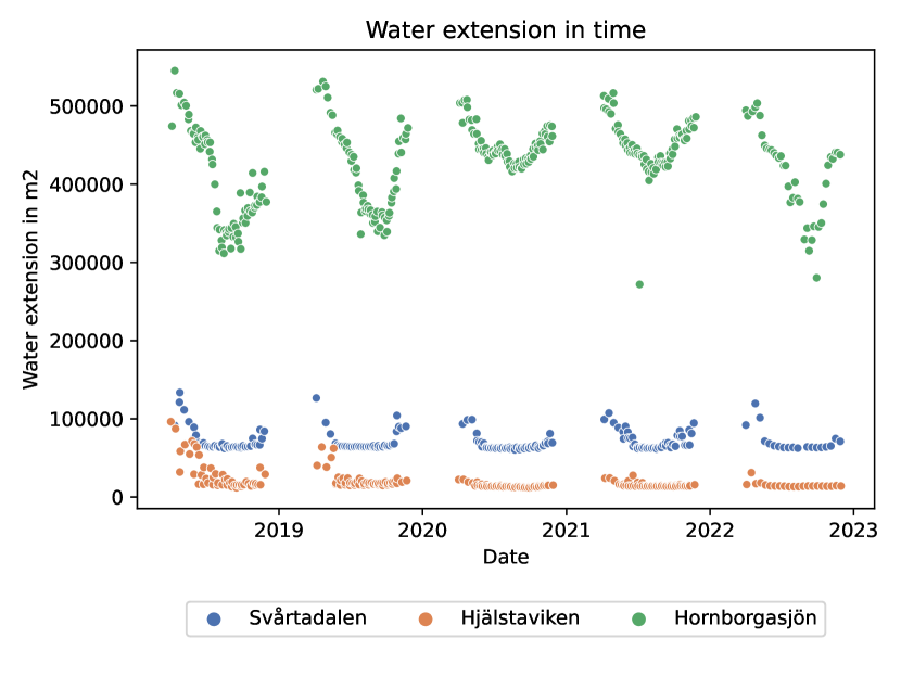
Figure 7: Dots indicate the water extension of three Swedish wetlands over 2018-2022. Only the months of April through November are considered.

To underscore the accuracy of DeepAqua, Figure 8 offers predictions for the three study areas across different months. The leftmost column displays the input SAR image, while the rightmost presents manually annotated ground truth. Intermediate columns feature predictions from our model variations, particularly on DeepAqua-NDWI due to its superior performance.

The top row captures the Svrtadalen wetland during summer in July 4th, 2018. The Otsu method’s difficulty with speckle noise is evident, though filtering mitigates some of this. The DeepAqua model appears resilient to this noise and aligns closely with the ground truth. The middle row captures the Hjälstaviken wetland during autumn on October 4th, 2020. This image is more noisy than the previous one, causing challenges for the Otsu method. Instead of reducing the noise, the Gaussian filter amplifies it. DeepAqua deals well with the noise, offering clear predictions. However, as indicated by the red pixels, some areas at the top of the image missed water detection. The bottom row shows the Hornborgasjön wetland in spring on April 19th, 2021. Both Otsu methods falter due to noise, while DeepAqua largely avoids it, though some FP emerge, as indicated by the cyan pixels.

Notably, DeepAqua accurately predicts surface water extent and identifies “land islands” within the wetlands. While it is not flawless, with some FP and FN errors evident, its noise reduction capability is commendable and achieved without resorting to additional filtering or preprocessing. As the red and cyan pixels in Figure 8, errors often appear around wetland shores or where water levels are low. In these regions, differentiating between water and soil in SAR images can be challenging due to the mixed signals from the water-soil interface. We emphasize that DeepAqua does not use filtering or pre-processing techniques on the SAR images.

	SAR image	Otsu	Otsu + filter	DeepAqua	Ground truth
A
B
C

Figure 8: Illustration of the performance of our model for different areas and times of the year: Svrtadalen, July 4th, 2018 (A); Hjälstaviken, October 4th, 2020; and Hornborgasjön April 19th, 2021 (C). From left to right: original SAR images, segmentation using Otsu’s method, segmentation using Otsu’s method with a Gaussian filter, segmentation using DeepAqua, and manually annotated data. Green pixels denote TP, cyan pixels denote FP, red pixels denote FN and black pixels denote TN.

To summarize, DeepAqua excels in recognizing water signatures from SAR images. While the method effectively tracks wetland transitions over time, it does not inherently distinguish between open and vegetated waters due to SAR’s imaging nature. Although not the primary focus, coupling our approach with water index methods like NDWI can differentiate these water types. However, we recommend exploring radar sensors with more extended wavelengths than the C-band for dense vegetation like mangroves.

6 Conclusion

We present DeepAqua, which is a novel method that uses cross-modal knowledge distillation to train a CNN for semantic segmentation of water in SAR imagery without requiring annotated data. Our method consists of two models: a teacher model that creates NDWI water masks from optical images and a student model that learns to segment water in SAR images. We used U-Net to implement the student model. The teacher and student models are trained jointly by minimizing the Dice loss between their outputs. Our experiments confirmed that our model can accurately segment images, confidently detecting water. The model here is trained and tested in a marsh wetland environment. However, it can be applied to wetlands with emerging vegetation allowing the penetration of C-Band SAR signals. Future studies may adapt the approach for radar sensors with longer wavelengths to expand the applicability in wetlands with larger vegetation, such as Mangroves. The use of this model can aid applications where water detection is crucial, such as flooding detection, river and lake mapping, and water availability assessments in time and space.

References

- Banks et al. (2019) Banks, S., White, L., Behnamian, A., Chen, Z., Montpetit, B., Brisco, B., Pasher, J., Duffe, J., 2019. Wetland classification with multi-angle/temporal SAR using random forests. Remote Sens. 11, 670.
- Beyer et al. (2022) Beyer, L., Zhai, X., Royer, A., Markeeva, L., Anil, R., Kolesnikov, A., 2022. Knowledge distillation: A good teacher is patient and consistent, in: Proc. IEEECVF Conf. Comput. Vis. Pattern Recognit., pp. 10925–10934.
- Brown et al. (2022) Brown, C.F., Brumby, S.P., Guzder-Williams, B., Birch, T., Hyde, S.B., Mazzariello, J., Czerwinski, W., Pasquarella, V.J., Haertel, R., Ilyushchenko, S., et al., 2022. Dynamic world, near real-time global 10 m land use land cover mapping. Scientific Data 9, 251.
- Carvalho Júnior et al. (2011) Carvalho Júnior, O.A., Guimarães, R.F., Gillespie, A.R., Silva, N.C., Gomes, R.A., 2011. A new approach to change vector analysis using distance and similarity measures. Remote Sensing 3, 2473–2493.
- Cui et al. (2020) Cui, B., Zhang, Y., Li, X., Wu, J., Lu, Y., 2020. WetlandNet: Semantic segmentation for remote sensing images of coastal wetlands via improved UNet with deconvolution, in: Genet. Evol. Comput. Proc. Thirteen. Int. Conf. Genet. Evol. Comput. Novemb. 1–3 2019 Qingdao China 13, Springer. pp. 281–292.
- Dang and Li (2021) Dang, B., Li, Y., 2021. Msresnet: Multiscale residual network via self-supervised learning for water-body detection in remote sensing imagery. Remote Sensing 13, 3122.
- Dang et al. (2020) Dang, K.B., Nguyen, M.H., Nguyen, D.A., Phan, T.T.H., Giang, T.L., Pham, H.H., Nguyen, T.N., Tran, T.T.V., Bui, D.T., 2020. Coastal wetland classification with deep U-Net convolutional networks and Sentinel-2 imagery: A case study at the Tien Yen estuary of Vietnam. Remote Sens. 12, 3270.
- Deng et al. (2009) Deng, J., Dong, W., Socher, R., Li, L.J., Li, K., Fei-Fei, L., 2009. Imagenet: A large-scale hierarchical image database, in: 2009 IEEE Conf. Comput. Vis. Pattern Recognit., Ieee. pp. 248–255.
- Deng et al. (2022) Deng, X., Zheng, J., Zhang, Z., 2022. Personalized education: Blind knowledge distillation, in: Comput. Vision–ECCV 2022 17th Eur. Conf. Tel Aviv Isr. Oct. 23–27 2022 Proc. Part XXXIV, Springer. pp. 269–285.
- Dice (1945) Dice, L.R., 1945. Measures of the amount of ecologic association between species. Ecology 26, 297–302.
- Everingham et al. (2015) Everingham, M., Eslami, SM., Van Gool, L., Williams, C.K., Winn, J., Zisserman, A., 2015. The pascal visual object classes challenge: A retrospective. Int. J. Comput. Vis. 111, 98–136.
- Feyisa et al. (2014) Feyisa, G.L., Meilby, H., Fensholt, R., Proud, S.R., 2014. Automated water extraction index: A new technique for surface water mapping using landsat imagery. Remote sensing of environment 140, 23–35.
- Garcia-Garcia et al. (2018) Garcia-Garcia, A., Orts-Escolano, S., Oprea, S., Villena-Martinez, V., Martinez-Gonzalez, P., Garcia-Rodriguez, J., 2018. A survey on deep learning techniques for image and video semantic segmentation. Appl. Soft Comput. 70, 41–65.
- Geudtner et al. (2014) Geudtner, D., Torres, R., Snoeij, P., Davidson, M., Rommen, B., 2014. Sentinel-1 system capabilities and applications, in: 2014 IEEE Geosci. Remote Sens. Symp., IEEE. pp. 1457–1460.
- Goodfellow et al. (2020) Goodfellow, I., Pouget-Abadie, J., Mirza, M., Xu, B., Warde-Farley, D., Ozair, S., Courville, A., Bengio, Y., 2020. Generative adversarial networks. Commun. ACM 63, 139–144.
- Gorelick et al. (2017) Gorelick, N., Hancher, M., Dixon, M., Ilyushchenko, S., Thau, D., Moore, R., 2017. Google Earth Engine: Planetary-scale geospatial analysis for everyone. Remote Sens. Environ. doi:10.1016/j.rse.2017.06.031.
- Gunnarsson and Löfroth (2014) Gunnarsson, U., Löfroth, M., 2014. The Swedish wetland survey: compiled excerpts from the national final report. Naturvrdsverket.
- Hardy et al. (2019) Hardy, A., Ettritch, G., Cross, D.E., Bunting, P., Liywalii, F., Sakala, J., Silumesii, A., Singini, D., Smith, M., Willis, T., et al., 2019. Automatic detection of open and vegetated water bodies using Sentinel 1 to map African malaria vector mosquito breeding habitats. Remote Sens. 11, 593.
- He et al. (2016) He, K., Zhang, X., Ren, S., Sun, J., 2016. Deep residual learning for image recognition, in: Proc. IEEE Conf. Comput. Vis. Pattern Recognit., pp. 770–778.
- Hinton et al. (2015) Hinton, G., Vinyals, O., Dean, J., 2015. Distilling the knowledge in a neural network. ArXiv Prepr. ArXiv150302531 arXiv:1503.02531.
- Hosseiny et al. (2021) Hosseiny, B., Mahdianpari, M., Brisco, B., Mohammadimanesh, F., Salehi, B., 2021. WetNet: A spatial–temporal ensemble deep learning model for wetland classification using sentinel-1 and sentinel-2. IEEE Trans. Geosci. Remote Sens. 60, 1–14.
- Hu et al. (2020) Hu, H., Xie, L., Hong, R., Tian, Q., 2020. Creating something from nothing: Unsupervised knowledge distillation for cross-modal hashing, in: Proc. IEEECVF Conf. Comput. Vis. Pattern Recognit., pp. 3123–3132.
- Jamali and Mahdianpari (2022) Jamali, A., Mahdianpari, M., 2022. Swin transformer and deep convolutional neural networks for coastal wetland classification using sentinel-1, sentinel-2, and LiDAR data. Remote Sens. 14, 359.
- Jamali et al. (2021a) Jamali, A., Mahdianpari, M., Brisco, B., Granger, J., Mohammadimanesh, F., Salehi, B., 2021a. Deep Forest classifier for wetland mapping using the combination of Sentinel-1 and Sentinel-2 data. GIScience Remote Sens. 58, 1072–1089.
- Jamali et al. (2021b) Jamali, A., Mahdianpari, M., Brisco, B., Granger, J., Mohammadimanesh, F., Salehi, B., 2021b. Wetland mapping using multi-spectral satellite imagery and deep convolutional neural networks: A case study in Newfoundland and Labrador, Canada. Can. J. Remote Sens. 47, 243–260.
- Jamali et al. (2022) Jamali, A., Mahdianpari, M., Brisco, B., Mao, D., Salehi, B., Mohammadimanesh, F., 2022. 3DUNetGSFormer: A deep learning pipeline for complex wetland mapping using generative adversarial networks and Swin transformer. Ecol. Inf. 72, 101904.
- Jaramillo et al. (2019) Jaramillo, F., Desormeaux, A., Hedlund, J., Jawitz, J.W., Clerici, N., Piemontese, L., Rodríguez-Rodriguez, J.A., Anaya, J.A., Blanco-Libreros, J.F., Borja, S., Celi, J., Chalov, S., Chun, K.P., Cresso, M., Destouni, G., Dessu, S.B., Di Baldassarre, G., Downing, A., Espinosa, L., Ghajarnia, N., Girard, P., Gutiérrez, A.G., Hansen, A., Hu, T., Jarsjö", J., Kalantari, Z., Labbaci, A., Licero-Villanueva, L., Livsey, J., Machotka, E., McCurley, K., Palomino-Ángel, S., Pietron, J., Price, R., Ramchunder, S.J., Ricaurte-Villota, C., Ricaurte, L.F., Dahir, L., Rodríguez, E., Salgado, J., Sannel, A.B.K., Santos, A.C., Seifollahi-Aghmiuni, S., Sjöberg, Y., Sun, L., Thorslund, J., Vigouroux, G., Wang-Erlandsson, L., Xu, D., Zamora, D., Ziegler, A.D., Åhlén, I., 2019. Priorities and interactions of sustainable development goals (sdgs) with focus on wetlands. Water 11. URL: https://www.mdpi.com/2073-4441/11/3/619, doi:10.3390/w11030619.
- Ji et al. (2009) Ji, L., Zhang, L., Wylie, B., 2009. Analysis of dynamic thresholds for the normalized difference water index. Photogrammetric Engineering & Remote Sensing 75, 1307–1317.
- Jiang et al. (2019) Jiang, Z., Von Ness, K., Loisel, J., Wang, Z., 2019. ArcticNet: A deep learning solution to classify arctic wetlands. ArXiv Prepr. ArXiv190600133 arXiv:1906.00133.
- Kang et al. (2021) Kang, J., Guan, H., Peng, D., Chen, Z., 2021. Multi-scale context extractor network for water-body extraction from high-resolution optical remotely sensed images. International Journal of Applied Earth Observation and Geoinformation 103, 102499.
- Karra et al. (2021) Karra, K., Kontgis, C., Statman-Weil, Z., Mazzariello, J.C., Mathis, M., Brumby, S.P., 2021. Global land use/land cover with sentinel 2 and deep learning, in: 2021 IEEE international geoscience and remote sensing symposium IGARSS, IEEE. pp. 4704–4707.
- Kingma and Ba (2015) Kingma, D.P., Ba, J., 2015. Adam: A method for stochastic optimization, in: Bengio, Y., LeCun, Y. (Eds.), 3rd Int. Conf. Learn. Represent. ICLR 2015 San Diego CA USA May 7-9 2015 Conf. Track Proc.
- Krizhevsky et al. (2017) Krizhevsky, A., Sutskever, I., Hinton, G.E., 2017. Imagenet classification with deep convolutional neural networks. Commun. ACM 60, 84–90.
- LeCun et al. (2015) LeCun, Y., Bengio, Y., Hinton, G., 2015. Deep learning. nature 521, 436–444.
- Li et al. (2020) Li, N., Lv, X., Xu, S., Li, B., Gu, Y., 2020. An improved water surface images segmentation algorithm based on the otsu method. Journal of Circuits, Systems and Computers 29, 2050251.
- Liu et al. (2021) Liu, Z., Lin, Y., Cao, Y., Hu, H., Wei, Y., Zhang, Z., Lin, S., Guo, B., 2021. Swin transformer: Hierarchical vision transformer using shifted windows, in: Proc. IEEECVF Int. Conf. Comput. Vis., pp. 10012–10022.
- Mahdianpari et al. (2018) Mahdianpari, M., Salehi, B., Rezaee, M., Mohammadimanesh, F., Zhang, Y., 2018. Very deep convolutional neural networks for complex land cover mapping using multispectral remote sensing imagery. Remote Sens. 10, 1119.
- Matthews et al. (1993) Matthews, G.V.T., et al., 1993. The ramsar convention on wetlands: its history and development, Ramsar Convention Bureau Gland.
- McFeeters (1996) McFeeters, S.K., 1996. The use of the Normalized Difference Water Index (NDWI) in the delineation of open water features. Int. J. Remote Sens. 17, 1425–1432.
- Mondini et al. (2021) Mondini, A.C., Guzzetti, F., Chang, K.T., Monserrat, O., Martha, T.R., Manconi, A., 2021. Landslide failures detection and mapping using Synthetic Aperture Radar: Past, present and future. Earth Sci. Rev. 216, 103574.
- Onojeghuo and Onojeghuo (2023) Onojeghuo, A.O., Onojeghuo, A.R., 2023. Wetlands mapping with deep ResU-Net CNN and open-access multisensor and multitemporal satellite data in alberta’s parkland and grassland region. Remote Sens. Earth Syst. Sci. , 1–16.
- Otsu (1979) Otsu, N., 1979. A threshold selection method from gray-level histograms. IEEE Trans. Syst. Man Cybern. 9, 62–66.
- Paszke et al. (2019) Paszke, A., Gross, S., Massa, F., Lerer, A., Bradbury, J., Chanan, G., Killeen, T., Lin, Z., Gimelshein, N., Antiga, L., et al., 2019. Pytorch: An imperative style, high-performance deep learning library. Adv. Neural Inf. Process. Syst. 32.
- Pham et al. (2022) Pham, H.N., Dang, K.B., Nguyen, T.V., Tran, N.C., Ngo, X.Q., Nguyen, D.A., Phan, T.T.H., Nguyen, T.T., Guo, W., Ngo, H.H., 2022. A new deep learning approach based on bilateral semantic segmentation models for sustainable estuarine wetland ecosystem management. Sci. Total Environ. 838, 155826.
- Reis et al. (2021) Reis, L.G.d.M., Souza, W.d.O., Ribeiro Neto, A., Fragoso Jr, C.R., Ruiz-Armenteros, A.M., Cabral, J.J.d.S.P., Montenegro, S.M.G.L., 2021. Uncertainties involved in the use of thresholds for the detection of water bodies in multitemporal analysis from landsat-8 and sentinel-2 images. Sensors 21, 7494.
- Rezaee et al. (2018) Rezaee, M., Mahdianpari, M., Zhang, Y., Salehi, B., 2018. Deep convolutional neural network for complex wetland classification using optical remote sensing imagery. IEEE J. Sel. Topics Appl. Earth Observ. Remote Sens. 11, 3030–3039.
- Ronneberger et al. (2015) Ronneberger, O., Fischer, P., Brox, T., 2015. U-net: Convolutional networks for biomedical image segmentation, in: Int. Conf. Med. Image Comput. Comput.-Assist. Interv., Springer. pp. 234–241.
- Shorten and Khoshgoftaar (2019) Shorten, C., Khoshgoftaar, T.M., 2019. A survey on image data augmentation for deep learning. J. Big Data 6, 1–48.
- Shurrab and Duwairi (2022) Shurrab, S., Duwairi, R., 2022. Self-supervised learning methods and applications in medical imaging analysis: A survey. PeerJ Comput. Sci. 8, e1045.
- Slagter et al. (2020) Slagter, B., Tsendbazar, N.E., Vollrath, A., Reiche, J., 2020. Mapping wetland characteristics using temporally dense Sentinel-1 and Sentinel-2 data: A case study in the St. Lucia wetlands, South Africa. Int. J. Appl. Earth Obs. Geoinf. 86, 102009.
- Soomro et al. (2018) Soomro, T.A., Afifi, A.J., Gao, J., Hellwich, O., Paul, M., Zheng, L., 2018. Strided U-Net model: Retinal vessels segmentation using dice loss, in: 2018 Digit. Image Comput. Tech. Appl. DICTA, IEEE. pp. 1–8.
- Tan et al. (2023) Tan, J., Tang, Y., Liu, B., Zhao, G., Mu, Y., Sun, M., Wang, B., 2023. A self-adaptive thresholding approach for automatic water extraction using sentinel-1 sar imagery based on otsu algorithm and distance block. Remote Sensing 15, 2690.
- Thorslund et al. (2017) Thorslund, J., Jarsjo, J., Jaramillo, F., Jawitz, J.W., Manzoni, S., Basu, N.B., Chalov, S.R., Cohen, M.J., Creed, I.F., Goldenberg, R., et al., 2017. Wetlands as large-scale nature-based solutions: Status and challenges for research, engineering and management. Ecological Engineering 108, 489–497.
- Tsyganskaya et al. (2018) Tsyganskaya, V., Martinis, S., Marzahn, P., Ludwig, R., 2018. Detection of temporary flooded vegetation using Sentinel-1 time series data. Remote Sens. 10, 1286.
- Wu et al. (2018) Wu, W., Li, Q., Zhang, Y., Du, X., Wang, H., 2018. Two-step urban water index (tsuwi): A new technique for high-resolution mapping of urban surface water. Remote sensing 10, 1704.
- Xu et al. (2020) Xu, G., Liu, Z., Li, X., Loy, C.C., 2020. Knowledge distillation meets self-supervision, in: Comput. Vision–ECCV 2020 16th Eur. Conf. Glasg. UK August 23–28 2020 Proc. Part IX, Springer. pp. 588–604.
- Xu (2006) Xu, H., 2006. Modification of normalised difference water index (ndwi) to enhance open water features in remotely sensed imagery. International journal of remote sensing 27, 3025–3033.
- Yao et al. (2015) Yao, F., Wang, C., Dong, D., Luo, J., Shen, Z., Yang, K., 2015. High-resolution mapping of urban surface water using zy-3 multi-spectral imagery. Remote Sensing 7, 12336–12355.
- Zanaga et al. (2022) Zanaga, D., Van De Kerchove, R., Daems, D., De Keersmaecker, W., Brockmann, C., Kirches, G., Wevers, J., Cartus, O., Santoro, M., Fritz, S., Lesiv, M., Herold, M., Tsendbazar, N.E., Xu, P., Ramoino, F., Arino, O., 2022. Esa worldcover 10 m 2021 v200. URL: https://doi.org/10.5281/zenodo.7254221, doi:10.5281/zenodo.7254221.
- Zhou et al. (2020) Zhou, S., Kan, P., Silbernagel, J., Jin, J., 2020. Application of image segmentation in surface water extraction of freshwater lakes using radar data. ISPRS International Journal of Geo-Information 9, 424.