The dark matter unitarity bound at NLO

Abstract

We reexamine the consequences of perturbative unitarity on dark matter freeze-out when both Sommerfeld enhancement and bound state formation affect dark matter annihilations. At leading order (LO) the annihilation cross-section is infrared dominated and the connection between the unitarity bound and the upper bound on the dark matter mass depends only on how the different partial waves are populated. We compute how this picture is modified at next-to-leading order (NLO) with the goal of assigning a reliable theory uncertainty to the freeze-out predictions. We explicitly compute NLO corrections in a simple model with abelian gauge interactions and provide an estimate of the theoretical uncertainty for the thermal masses of heavy electroweak $n$-plets. Along the way, we clarify the regularization and matching procedure necessary to deal with singular potentials in quantum mechanics with a calculable relativistic UV completion.

I Introduction

Among the plethora of dark matter (DM) production mechanisms, a minimal and predictive setup is DM thermal freeze-out where the DM is in thermal contact with the Standard Model (SM) bath in the early Universe, and its abundance today is set by 2-2 annihilations into SM or dark sector states.

This simple framework makes it possible to derive an upper bound on the DM mass from the perturbative unitarity of the annihilation cross-section as was first done in Ref. [1]. The unitarity of the S-matrix bounds from above every single partial wave contributing to the annihilation cross-section. At a given order in the perturbative expansion, this bound can be recast into a maximal value of the gauge coupling. The latter can then be translated into an upper bound on the DM mass through the requirement that the total annihilation cross-section should deplete the DM abundance to match the measured relic density today.

When long-range interactions are at work, non-relativistic (NR) quantum mechanical effects significantly alter the DM annihilation cross-section inducing an overall enhancement which is dubbed Sommerfeld enhancement (SE) in the literature [2, 3, 4, 5, 6, 7] typically accompanied by the bound state formation (BSF) during the annihilation process [8, 9, 10, 11]. Since these effects dominate the annihilation cross-section it is crucial to understand their behavior once we approach the perturbative unitarity bound (PUB). This question is the main focus of this paper.

Approaching the PUB, NLO corrections should become important and their relative size compared to the LO contributions gives a reliable estimate of the expected theory uncertainty. We then study the behavior of NLO corrections to the non-relativistic potential making use of the general results from Ref. [12, 13, 14]. We systematically include corrections generated both by the infrared (IR) and ultraviolet (UV) dynamics.

Our analysis allows us to reliably assign a theoretical uncertainty to the freeze-out predictions. Even though our results are general, we use a simple dark QED model to illustrate the impact of NLO corrections. We will comment on how this analysis allows us to assign a more reliable theory error to the electroweak WIMPs thermal masses derived in Ref. [15, 16].

Our paper is structured as follows. In Sec. II we summarize the relevant ingredients for the LO freeze-out computation and discuss the PUB at LO. In Sec. III we develop the tools to account for both IR (Sec. III.1) and UV NLO corrections (Sec. III.2). In Sec. IV we then illustrate the importance of our corrections in a simple dark QED model. In Sec. V we conclude. In Appendix A we illustrate the general strcture of UV NLO potentials while in Appendix B we illustrate our regularization and matching procedure in the simple case of the Coulomb potential. In Appendix C we collect useful formulas about bound state formation.

II The Unitarity bound at LO

We first discuss DM annihilation at LO. We illustrate SE in Sec. II.1 and BSF in Sec. II.2. The DM PUB at LO and its consequences are considered in Sec. II.3. We decompose the annihilation channels in eigenvalues of the total angular momentum $\vec{J}=\vec{L}+\vec{S}$, where $\vec{L}$ is the angular momentum and $\vec{S}$ is the internal spin.

Since the freeze-out happens at NR velocities the annihilation channels with $\vec{L}\neq 0$ are velocity suppressed. We can then focus on s-wave annihilation and set $\vec{L}=0$ and $\vec{J}=\vec{S}$. We consider the DM to be a scalar or a fermion, where in the latter case both $j=1$ and $j=0$ channels contribute to the s-wave annihilation. For simplicity, we take the DM to be in thermal contact with the SM in the early Universe so that the freeze-out dynamics is controlled by a thermal bath with a number of light degrees of freedom at the freeze-out temperature $g_{*}^{\text{f.o.}}\equiv g_{*}(T_{\text{f.o.}})$ possibly different than the SM one.

II.1 Hard cross-section and Sommerfeld enhancement

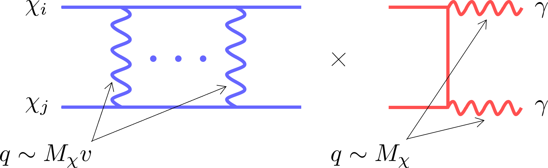
Figure 1: Sketch of the annihilation rate process. The red diagram shows the hard annihilation cross-section where the particles in the final state carry most of the DM energy. The blue diagram includes soft exchanges with momentum $p=M_{\chi}v$ which get resummed by the non-relativistic potential.

In the NR limit the dynamics of annihilation is captured by the Schröedinger equation for the system of the pair of annihilating particles $\phi_{j,i}(r)$. Here $j=s$ selects a given total angular momentum channel at $l=0$ while the index $i$ stands for other possible internal degrees of freedom. The Schröedinger equation reads

$$-\frac{\nabla^{2}\phi_{j,i}}{M_{\chi}}+\left[V_{i}^{\text{LO}}-i\frac{\sigma_{j,i}^{h}v}{2}\delta^{3}(\vec{r})\right]\phi_{j,i}=\frac{M_{\chi}v^{2}}{4}\phi_{j,i}\,,$$ (1)

the imaginary part of the potential in the squared brackets is related through the optical theorem to the “hard” annihilation cross-sections $\sigma_{j,i}^{h}$ which describes the processes whose decay products carry most of the DM energy as shown in Fig. 1. Upon projecting into radial wave functions, the kinetic term will also generate the usual centrifugal barrier $1/r^{2}$.

At small velocities, $v\ll\alpha$, the dynamics of DM is affected by the long-range interactions encoded in the non-relativistic potentials $V_{i}^{\text{LO}}$. At LO in $\alpha$ and $v$, the potential takes the standard Coulomb form

$$V^{\text{LO}}_{i}(r)=\lambda_{i}\frac{\alpha}{r}\ ,$$ (2)

where $\lambda_{i}$ is a channel-dependent number (which we assume to be spin independent) that can be negative (positive) for attractive (repulsive) potentials.

The full, non-perturbative annihilation cross-section can be computed by solving Eq. (1). The contribution of the modified wave function to the annihilation cross-section can be read from the divergence of the probability current $\vec{j}_{j,i}(\vec{r})=\frac{2}{M_{\chi}}\Im[\phi_{j,i}^{\dagger}\vec{\nabla}\phi_{j,i}]$

$$\sigma_{j,i}v=-\int\mathrm{d}^{3}r\vec{\nabla}\cdot\vec{j}_{j,i}(\vec{r})\simeq\sigma^{h}_{j,i}v|\phi_{i}(0)|^{2}\ ,$$ (3)

where $S_{E}^{i}\equiv|\phi_{i}(0)|^{2}$ is the so-called Sommerfeld enhancement (SE) and $\phi_{i}(x)$ is the spin-independent solution of the Schröedinger equation Eq. 1 neglecting the contribution from the hard process. The boundary conditions for $\phi_{i}$ are requiring regularity at the origin and to recover the asymptotic scattering waves away from the potential.

A simple way to compute the SE is to rewrite Eq. (1) as a first order differential equation for $h_{j,i}(r)=\phi_{j,i}^{\prime}(r)/\phi_{j,i}(r)$

$$\frac{h^{\prime}_{j,i}}{M_{\chi}}+h^{2}_{j,i}-\left[V_{i}^{\text{LO}}-i\frac{\sigma_{j,i}^{h}v}{2}\delta^{3}(\vec{r})\right]=\frac{M_{\chi}v^{2}}{4}\,,$$ (4)

with boundary condition $h(r\rightarrow\infty)=iM_{\chi}v/2$. In terms of the new variable the SE in Eq. (3) can be written as $S_{E}^{i}=2\Im[h_{i}(0)]/(M_{\chi}v)$ under the same approximation of Eq. (3). We will use this formulation in Sec. III.1.

Another nice way of writing the SE is to introduce the reduced radial wave function for $l=0$, $\chi_{j,i}(r)=r\phi_{j,i}(r)$ and define the dimensionless variable $x=rM_{\chi}$ and the rescaled potential $V_{i}^{\text{LO}}=M_{\chi}\mathcal{V}^{\text{LO}}_{i}$ so that Eq. (1) becomes

$$-\chi^{\prime\prime}_{j,i}+\left[\mathcal{V}_{i}^{\text{LO}}-i\frac{\sigma^{h}_{j,i}v}{2M_{\chi}}\delta^{3}(\vec{x})\right]\chi_{j,i}=\frac{v^{2}}{4}\chi_{j,i}\ .$$ (5)

Choosing carefully the boundary conditions we can get equivalent expressions of the SE in terms of the reduced wave function. For instance taking $\chi(0)\propto x$ and $\chi_{i}(\infty)=\sin(xv/2+\delta_{0}^{i})$ we get $S_{E}^{i}=|2\chi_{i}^{\prime}(0)/v|^{2}$. Alternatively, imposing $\chi(0)=xv/2$ we get $\chi_{i}(\infty)=\sin(xv/2+\delta_{0}^{i})/\sqrt{S_{E}}$. This latter formulation will be useful in Sec. III.2.

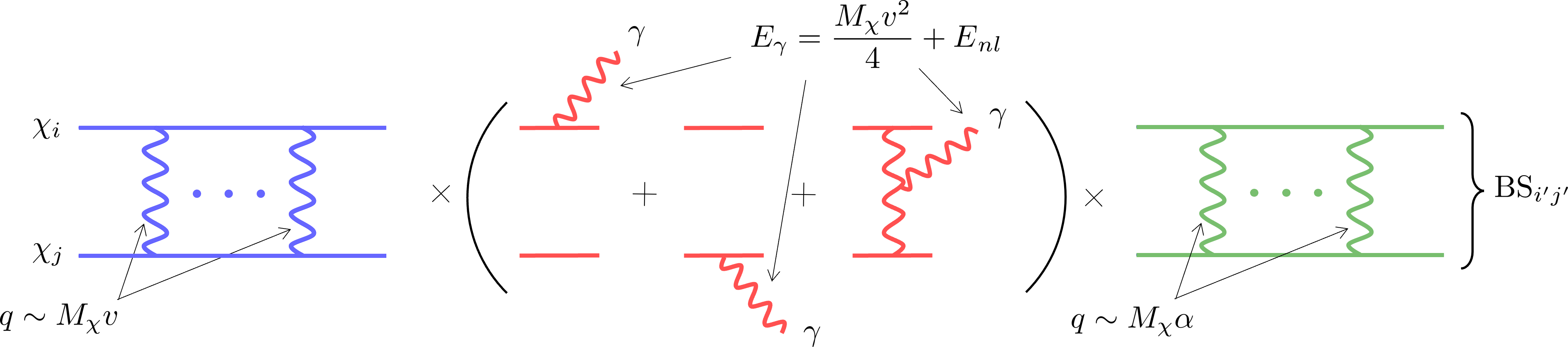
Figure 2: Sketch of the bound state formation process. The red diagram shows the fundamental emission process, where a vector with energy given approximately by the binding energy of the BS is emitted from the DM line (dipole) or from the internal vector line (non-abelian). The blue (green) ladder diagram includes soft photon exchanges with momentum $p=M_{\chi}v$ ($p=M_{\chi}\alpha$) which get resummed by the non-relativistic potential at LO into the scattering (bound state) wave function.

For a Coulomb potential, the $S_{E}$ takes the simple analytic form

$$S_{E}^{i}|_{\text{LO}}=\frac{2\pi\lambda_{i}\alpha}{v}\frac{1}{1-e^{-\frac{2\pi\lambda_{i}\alpha}{v}}}\ ,$$ (6)

which strongly enhances (or suppresses) the $l=0$ annihilation cross-section when $v<\lambda_{i}\alpha$. The annihilation cross-section for a single $j$ wave can then be parametrically written at LO as

$$\sigma^{j}_{\text{ann}}v=\sum_{i}\sigma_{j,i}v=\frac{2\pi^{2}\alpha^{3}}{vM_{\chi}^{2}}c_{\text{ann}}^{j}|_{\text{LO}}\ ,$$ (7)

where we defined $c_{\text{ann}}^{j}|_{\text{LO}}=\sum_{i}c_{j,i}^{h}\lambda_{i}$ and $c_{j,i}^{h}$ are $\mathcal{O}(1)$ coefficients encoding the LO contribution of the hard cross-section to the different channels and $\lambda_{i}$ are defined in Eq. 2.

II.2 Bound State Formation

In the NR regime typical of freeze-out, long-range interactions lead to a significant rate of BSF. Since these BS are not stable, BSF helps in depleting the DM abundance and thus affects the prediction of the DM mass.

At leading order in $\alpha$ and $v$, BSF occurs via emission of a single gauge boson through the process $\chi_{1,i}+\chi_{2,i^{\prime}}\rightarrow\text{BS}_{ff^{\prime}}+V^{a}$ described by a generalized dipole Hamiltonian derived in Ref. [19, 20, 10]. We can write the final BSF cross-section as

$$\sigma_{\text{BS}}^{i_{s}i_{b}}v=S_{\text{BS}}^{i_{s}i_{b}}\left(S_{E}^{i_{s}}\frac{\pi\alpha^{2}}{M_{\chi}^{2}}\right)\,,$$ (8)

where $S_{E}^{i_{s}}\simeq 2\pi\lambda_{i_{s}}\alpha/v$ is the SE corresponding to the incoming scattering state, while $S^{i_{s}i_{b}}_{\text{BS}}$ encodes the non-trivial coupling and velocity dependence coming from the overlap integral between the incoming scattering state $i_{s}$ and the outcoming bound state BS. We leave a detailed discussion of the overlap integrals to Appendix C.

II.3 Unitarity bound at LO

As a direct consequence of the unitarity of the $S$-matrix, the 2-2 annihilation cross-section in a given partial wave with total angular momentum $j$ is bounded from above by $\sigma_{j}\leq\pi(2j+1)/p^{2}$, where $p$ is the initial momentum of the annihilating particles. In the non-relativistic limit, $p^{2}=M_{\chi}^{2}v^{2}/4$ and the PUB can be written as

$$\sigma_{j}v\leq\frac{4\pi(2j+1)}{M_{\chi}^{2}v}\ ,$$ (9)

where this inequality does not require the existence of free asymptotic states and it is also satisfied for scattering processes in a Coulomb potential [21].

The annihilation cross-section at LO and in the limit $v\ll\alpha$ can be written as

$$\sigma_{j}v|_{\text{LO}}\simeq\frac{2\pi^{2}\alpha^{3}}{vM_{\chi}^{2}}\left[c_{\text{ann}}^{j}|_{\text{LO}}+c_{\text{BSF}}^{j}|_{\text{LO}}\right]\ \ ,$$ (10)

where the coefficients $c_{\text{ann}}^{j}|_{\text{LO}}$ and $c_{\text{BSF}}^{j}|_{\text{LO}}$ encode model dependent $\mathcal{O}(1)$ numbers controlling the annihilation cross-section and the BSF respectively. In particular, $c_{\text{BSF}}^{j}$ can be obtained from Eq. (8) by projecting onto a state with total angular momentum $j$.

The maximal coupling allowed by PUB at LO is

$$\alpha^{\text{max}}_{\text{LO}}=\text{Max}_{j}\left[\frac{2(2j+1)}{(c_{\text{ann}}^{j}|_{\text{LO}}+c_{\text{BSF}}^{j}|_{\text{LO}})\pi}\right]^{1/3}\ ,$$ (11)

where it is interesting to notice that the presence of the SE in the non-relativistic limit reduces the maximally allowed coupling by roughly one order of magnitude compared to the usual bound from the relativistic power counting.

To a good approximation, the solution of the DM Boltzmann equation is equivalent to require the freeze-out yield to be $Y_{\chi}^{\text{f.o}}\simeq\frac{H}{s\sum_{j}\langle\sigma_{j}v\rangle}$, where $s$ is the entropy density. Substituting $\alpha^{\text{max}}_{\text{LO}}$ in the freeze-out condition and requiring $\chi$ to account for the DM relic density today we get the maximal DM mass allowed by the PUB

$$M_{\text{max}}\simeq 131.7\text{ TeV}\left(\alpha^{\text{max}}_{\text{LO}}\right)^{3/2}\left(\sum_{j}(c_{\text{ann}}^{j}|_{\text{LO}}+c_{\text{BSF}}^{j}|_{\text{LO}})\right)^{1/2}\left(\frac{g_{*}^{\text{f.o.}}}{x_{\text{f.o}}}\right)^{1/4}\ ,$$ (12)

where we substituted the high temperature value of the SM degrees of freedom $g_{*}^{\text{SM}}\simeq 106.75$ and $x_{\text{f.o}}\equiv M_{\chi}/T_{\text{f.o.}}\simeq 29$ (see Ref. [22] for details about the dependence of $x_{\text{f.o}}$ on the model parameters).

If the annihilation is dominated by a single $j$-wave then Eq. (12) simplifies and the mass upper bound becomes independent on the model as derived in Ref. [1]. For example if the $j=0$ wave dominates we get $M_{\text{max}}^{J=0}=137\text{ TeV}$.

In practice, the dominance of a single $j$-wave is an irrealistic assumption in most of the freeze-out scenarios. The main reason is that BSF tends to equally distribute the cross-section in the lower $j$ channels. As a consequence, accounting for BSF generically makes $M_{\text{max}}$ larger with respect to the naive estimate because the contribution from BSF in Eq. (12) overcomes the tightening of the PUB on $\alpha$ in Eq. (11).

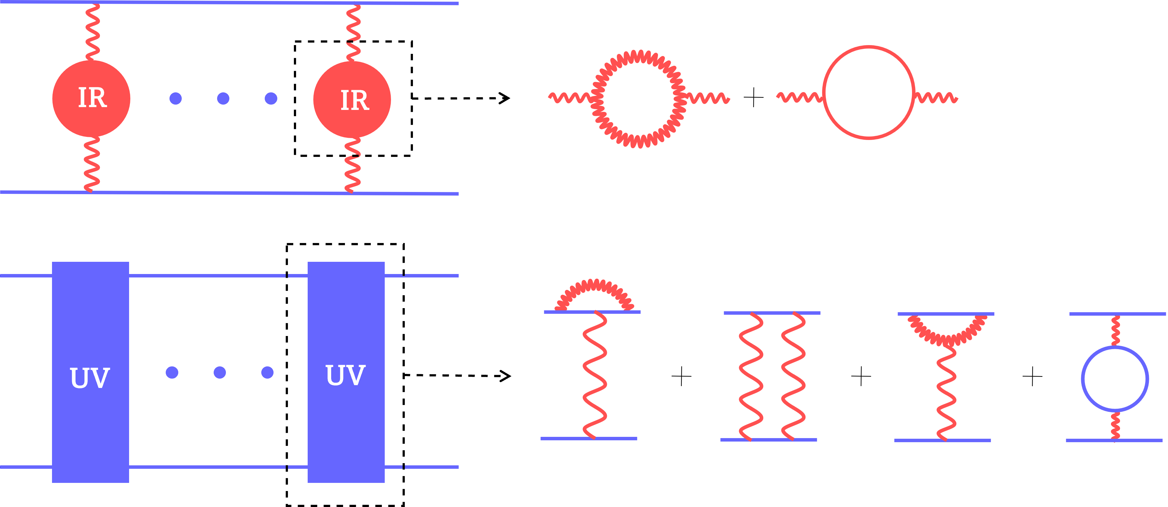
Figure 3: Sketchy representation of the IR contributions (top) and UV contributions (bottom) to the non-relativistic potentials at NLO. Red lines corresponds to IR degrees of freedom: fermions (solid) or gauge bosons (wiggly). Blue lines are instead heavy DM lines which we take to be scalar in this paper.

III NLO corrections

We study the NLO correction to the non-relativistic potential. These are expected to be the dominant NLO corrections approaching the unitarity bound at non-relativistic velocities $v\ll\alpha$ typical of freeze-out.

NLO corrections can arise from both IR and UV dynamics. The former originate from loops where only light degrees of freedom are involved and modify both the long-range and the short-range behavior of the Coulomb potential. On the contrary, UV contributions modify the short-range behavior of the Coulomb potential and are induced by the diagrams where also the heavy DM field $\chi$ flows in the loops. We schematically show both contributions in Fig. 3.

The dominant IR corrections can be approximated by the including the running coupling $\alpha(r)$ in the LO Coulomb potential [13, 14, 26]

$$V_{\rm NLO}^{\rm IR}=-\frac{\alpha(r)}{r}\ ,\quad\alpha(r)=\frac{\alpha}{1+\frac{\alpha}{2\pi}b^{\rm IR}\log(M_{\chi}r)}\ ,$$ (13)

where $b^{\rm IR}$ is the beta-function coefficient due to the states lighter than the DM mass running in the loops and we defined $\alpha$ to be the fine structure constant at the DM threshold $r=1/M_{\chi}$.

The UV corrections can be systematically encoded in the one-loop matching to the DM potential in Non-Relativistic QFT [12]. These thresholds can be organized as a series in powers of $1/M_{\chi}$ whose general form in Fourier space was derived in Ref. [12] up to order $\mathcal{O}(1/M_{\chi}^{2})$. In position space, the NLO potential reads

$$\Delta V_{\rm NLO}^{\rm UV}=-\frac{\alpha}{r}\left[\frac{V_{2}}{M_{\chi}r}+\frac{V_{3}}{M_{\chi}^{2}r^{2}}\right]+\frac{V_{D}\alpha}{M_{\chi}^{2}}\delta^{3}(\vec{r})\ .$$ (14)

where $V_{2}$, $V_{3}$, and $V_{D}$ are dimensionless coefficients that might depend on the annihilation channel (including the spin). $V_{3}$ and $V_{D}$ contain in general spin-dependent terms like spin-spin and spin-orbit interactions. These terms would induce transitions between states with different $l$ and $s$. In general, computing SE and BSF would then require solving a system of coupled Schröedinger equations. In the following, we consider the simple case of scalar DM, where these terms are zero. We provide more details on the general structure of the NLO potential in Appendix A.

Taking $r\sim 1/M_{\chi}v$ the size of the NLO corretions can be estimated as $\Delta V_{\text{NLO}}\sim\left[V_{2}v+(V_{3}+V_{D})v^{2}\right]V_{\text{LO}}$ with $V_{\text{LO}}\sim\alpha M_{\chi}v$ being the scaling of the Coulomb potential in Eq. (2). This estimate indicates that the inverse square potential dominates over the other NLO corrections as long as $v<V_{2}^{i}/(V_{3}^{i}+V_{D}^{i})$. The leading relativistic correction to the kinetic energy $M_{\chi}^{3}\Delta E_{\text{kin}}=p^{4}/8$ scales as $\Delta E_{\text{kin}}\sim M_{\chi}v^{4}$ and are negligible with respect to the correction to the potential as long as $v<(V_{2}\alpha)^{1/2}$ and $v<(V_{3}+V_{D})\alpha$ respectively. This shows that at low enough velocities, the leading NLO corrections can be encoded solely in the modifications of the potential in the Schröedinger equation.

We now present a systematic procedure to account for both IR and UV NLO corrections in the SE and in BSF.

III.1 IR contributions at NLO

The IR behavior of the NLO potential crucially depends on the sign of the IR beta-function coefficient $b_{\rm IR}$. Here we focus on IR free theories with $b_{\rm IR}>0$ whose NLO potential features a Landau pole at a position $r_{*}M_{\chi}=\exp(-\frac{2\pi}{b_{\rm IR}\alpha})$. The presence of a Landau pole prevents fixing boundary conditions at distances arbitrarily close to the origin.

The boundary condition is then set at a distance $r_{p}$ defined as $2\Im[h(r_{p})]/M_{\chi}v=(1-p)S_{E}$, where $p$ is an arbitrary parameter that controls the theoretical accuracy of our approximation. By inspecting the Schröedinger equation we can also estimate the value of $r_{p}$ which corresponds to the onset of the plateau of the SE: $p/r_{p}\approx 2(1+\pi)M_{\chi}\alpha$. The value of $r_{p}$ is velocity independent, as can be understood by noticing that at small distances the potential energy dominates over the kinetic energy. The larger is $p$ the further away we are from the saturation of the SE and the larger is our theoretical error.

As long as $r_{p}>r_{*}$, we can solve the Schröedinger equation with the resummed potential in Eq. (13), and compute the SE. For $\alpha_{\text{LO}}^{\text{max}}$ defined in Eq. (11) $r_{*}$ is the largest: $r_{*}(\alpha_{\text{LO}}^{\text{max}})=r_{*}|_{\text{max}}$. We can then fix $p$ to minimize the theoretical error at the PUB by defining $r_{\bar{p}}=r_{*}|_{\text{max}}$, which fixes the value of $p=\bar{p}$. This choice ensures the calculability of the SE up to the PUB. We can then estimate the theoretical error due to IR NLO effects by taking the difference of the SE between $r_{\bar{p}}$ and $2r_{\bar{p}}$ for any coupling: $\Delta S^{\text{IR}}_{E}=S_{E}(r_{\bar{p}})-S_{E}(2r_{\bar{p}})$. In Sec. IV we will apply this recipe to a simple toy model with abelian gauge interactions.

We now briefly comment on the impact of IR NLO corrections on BSF. The BS wave functions and binding energies can be computed at NLO using as an unperturbed basis the Coulombian BS and diagonalizing the matrix elements of the Hamiltonian $\mathcal{H}_{\text{NLO}}=\frac{p^{2}}{M_{\chi}}+V_{\text{NLO}}^{\text{IR}}(r)$, where $\mathcal{H}_{ij}^{l}\equiv\langle\Psi^{C}_{il}|\mathcal{H}|\Psi^{C}_{jl}\rangle$, with $|\Psi^{C}_{il}\rangle$ the Coulombian BS with principal quantum number $i$ and angular momentum $l$. The BS wave function and its binding energy are mostly sensitive to scales larger than the Bohr radius, $r\gtrsim\frac{1}{M_{\chi}\alpha}$. For this reason, the BS dynamics is insensitive to NLO corrections in theories with $\beta_{\text{IR}}>0$, where the deviations from the Coulomb behavior are larger at short scales. Conversely, we expect large NLO corrections to the BS dynamics in UV-free theories with $\beta_{\text{IR}}<0$. We leave a detailed study of this case for the future.

For $\beta_{\text{IR}}>0$, the BSF cross-section is mostly affected by NLO modifications of the scattering wave function. These correction affects mostly the formation of $p$-wave BS from a $s$-wave initial scattering state because scattering waves with angular momentum $l>0$ are screened from short-scale NLO corrections by the centrifugal potential. More details are given in Appendix C.

III.2 UV contributions at NLO

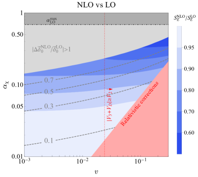
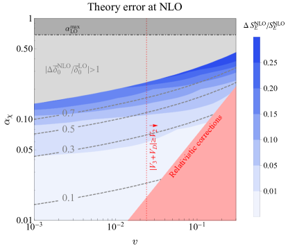
Figure 4: Behavior of the UV NLO corrections described in Sec. III.2 with $x_{\text{cut}}=1$. The red lines exhibit the power counting on the relativistic corrections discussed below Eq. (14). On the right of the red dashed line, the NLO potential cannot be approximated with a $1/r^{2}$ correction to the Coulomb potential while on the red shaded region the corrections to the kinetic energy become important and the non-relativistic description breaks down. The gray dashed lines show the NLO contribution to the UV phase in the Born approximation as defined in Eq. (25), normalized with respect to the LO one. In the gray shaded area the NLO contribution becomes larger than the LO one and the calculability of the phase breaks down. Left: The blue contours show the behavior of the mean value of the NLO SE normalized with respect with the LO SE. Right: The blue contours show the behavior of the theory error on the NLO SE due to the uncertainty on the UV phase determination as defined in Eq. (26).

The inclusion of the UV NLO corrections in Eq. (14) makes the Hamiltonian no longer bounded from below. Equivalently, the Schröedinger equation with $V_{\text{NLO}}^{\text{UV}}=V_{\text{LO}}+\Delta V_{\text{NLO}}^{\text{UV}}$ cannot be solved with normalizable solutions with boundary conditions at the origin. This poses the challenge of defining the SE in the presence of UV singular potential.

Following the approach of Ref. [17] (see also Ref. [27, 28] for similar techniques applied to nuclear physics), we regularize the full potential close to the origin with a well potential at distances $r<r_{\rm cut}\equiv x_{\rm cut}/M_{\chi}$. In terms of the dimensionless variable $x=rM_{\chi}$ we can define a dimensionless regularized potential

$$\mathcal{V}_{\text{reg}}(x)=\left\{\begin{aligned} &-\mathcal{V}_{\rm cut}(v,x_{\text{cut}}),\quad x<x_{\rm cut}\\ &\mathcal{V}_{\text{NLO}}^{\text{UV}}(x),\qquad\quad\ \ x>x_{\rm cut}\end{aligned}\right.\ ,$$ (15)

where $V_{\text{NLO}}^{\text{UV}}=M_{\chi}\mathcal{V}_{\text{NLO}}^{\text{UV}}$. The Schröedinger equation in Eq. (5) can be written by replacing the potential with the regularized one ($\mathcal{V}_{\text{LO}}\to\mathcal{V}_{\text{reg}}$) and the kinetic term with an arbitrary wave function renormalization ($\chi^{\prime\prime}\to Z_{\chi}\chi^{\prime\prime}$). In general, the depth of the potential well $-\mathcal{V}_{\rm cut}$ and the wave function renormalization $Z_{\chi}$ are functions of $x_{\text{cut}}$ and of $v$ and they should be fixed with appropriate renormalization conditions in order for the SE to be well defined.

Since the relativistic UV theory is calculable, the scattering phase can be explicitly computed and matched to the non-relativistic EFT as an input (see Ref. [29, 30] for a similar discussion in the context of scattering processes). At distances $x<x_{\rm cut}$, the $s$-wave scattering phase can be computed for a generic central potential in the Born approximation

$$\sin\bar{\delta}_{0}^{\text{NLO}}=-v\int_{0}^{x_{\text{cut}}}\mathrm{d}xx^{2}j_{0}^{2}(vx)\mathcal{V}_{\text{NLO}}(x)\ ,$$ (16)

where $j_{0}(x)$ is the regular, spherical Bessel function and $\mathcal{V}_{\text{NLO}}$ is the full NLO potential.

The UV scattering wave function can then be written as $\sin(vx+\bar{\delta}_{0})$ and it is then matched at $x=x_{\text{cut}}$ to the solution of the Schröedinger equation for $x<x_{\text{cut}}$ inside the potential well. Matching the logarithmic derivatives we get

$$\tan\left(\frac{vx_{\rm cut}}{2}+\bar{\delta}_{0}^{\text{NLO}}\right)=\frac{v}{2\Phi_{v}}\tan\left(x_{\rm cut}\Phi_{v}\right)\ ,$$ (17)

where we defined $\Phi_{v}\equiv\left(\frac{4\mathcal{V}_{\rm cut}+v^{2}}{4Z_{\chi}}\right)^{1/2}$. At fixed $x_{\text{cut}}=1$ and $v$, this matching condition fixes $\Phi_{v}$ in terms of $\bar{\delta}_{0}^{\text{NLO}}$ so that the solution inside the potential well is

$$\chi_{v}^{\text{in}}(x)=\frac{v}{2\Phi_{v}}\sin(\Phi_{v}x)\quad\text{for}\quad x<x_{\text{cut}}\$$ (18)

and can be matched at $x=x_{\text{cut}}$ to $\chi^{\text{out}}_{v}(x)$ which solves the Schröedinger equation for $x>x_{\text{cut}}$ with the potential in Eq. (15). This boundary condition alone is not sufficient to disentangle the SE from the asymptotic behavior of $\chi^{\text{out}}_{v}(x)$ which also depends on the wave function renormalization $Z_{\chi}$:

$$\lim_{x\to\infty}\chi_{v}^{\text{out}}(x)=\frac{\sin(xv+\delta)}{\sqrt{S_{E}(v)Z_{\chi}}}\ ,$$ (19)

where the phase $\delta$ depends on the long-range dynamics and has to be distinguished from the short-distance one in Eq. (16).

An independent relation is then obtained by requiring the SE to approach 1 at large velocities as suggested in Ref. [17]. In the $v\gg 1$ limit $\Phi_{v}\simeq 1/\sqrt{Z_{\chi}}$ so that the solution in Eq. (18) depends solely on the wave function renormalization. The latter can be fixed by requiring $S_{E}(v\gg 1)=1$ in Eq. (19):

$$\lim_{x\to\infty}\chi_{v}^{\text{out}}(x)\stackrel{{\scriptstyle[}}{{v}}\gg 1]{}{\simeq}\frac{\sin(vx+\delta)}{\sqrt{Z_{\chi}}}\ .$$ (20)

The matching condition in Eq. (17) admits different branches of solutions for $\Phi_{v}^{i}$ leaving the l.h.s of Eq. (17) unchanged [31]. However, only the solution in the first branch, defined by $0<\Phi_{v}<\pi/2x_{\rm cut}$, leads to a well-defined SE given the boundary conditions in Eq. (17) and Eq. (20).

This can be seen by considering the case of a very short-range potential with depth $\mathcal{V}_{\rm cut}$, which vanishes immediately outside the potential well $x>x_{\text{cut}}$. This is a limiting case that perfectly captures the physics in the extremely weakly coupled case. Since the wave function outside the well is just a plane wave one can follow our UV matching procedure to get the SE

$$S_{E}=\frac{1}{Z_{\chi}\cos^{2}(\Phi_{v}x_{\rm cut})\left[1+\frac{v^{2}}{4}\frac{\tan^{2}(\Phi_{v}x_{\rm cut})}{\Phi_{v}^{2}}\right]}\,.$$ (21)

Requiring $S_{E}(v\gg 1)=1$ as in Eq. (20) fixes $Z_{\chi}=1$.

Eq. (21) shows explicitly how the SE depends on the branch through the $1/\cos^{2}(\Phi_{v}x_{\rm cut})$ factor. Defining the $i$-th branch as the one with $(2i-1)\pi/2x_{\rm cut}<\Phi_{v}<(2i+1)\pi/2x_{\rm cut}$, with $i$ integer, the SE increases by moving to higher branches because the $\cos^{2}(\Phi_{v}x_{\rm cut})$ decreases. This behavior is inconsistent with the weak coupling limit ($\mathcal{V}_{\rm cut}\ll v^{2}/4$ in this simple setup) where we expect to recover $S_{E}\to 1$. This limit is realized in the first branch which we then select as the physical one.

The existence of a solution for Eq. (17) in the first branch is intimately related to the calculability of the UV phase. Indeed, in order to have a solution the l.h.s of the equation should be larger than the minimum of the r.h.s which is obtained for $\Phi_{v}\rightarrow 0$. This is possible only if $\bar{\delta}_{0}^{\text{NLO}}>0$ which is equivalent to requiring the LO Coulomb potential (which contributes positively to the scattering phase) to dominate over the NLO corrections (which contribute negatively) in Eq. (16). In the gray region in Fig. 4 a solution for the matching equation can only be found by pushing $x_{\text{cut}}>1$, hence enhancing the relative weight of the Coulomb potential with respect to the NLO corrections. This is done to extract the theory prediction on the SE and its error in this region as we show in Fig. (5).

Before leaving this section we comment on the UV NLO contributions to the BSF cross-section which is encoded in the deformation of the wave function of the initial scattering state and the on of the BS. While computing the latter is straightforward, in order to compute the first we generalize to discontinuous potentials the variable phase method introduced in [33] (see also [34, 8, 35]). This is described in Appendix C.4.

IV An abelian example

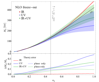
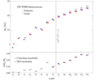
Figure 5: Left: DM thermal masses for LO and NLO corrections to the Coulomb potential in the dark QED model introduced in Sec. IV with $q_{\chi}=q_{e}=1$. The black line shows the LO prediction of the relic abundance. The red, blue, and green lines show the freeze-out prediction after the inclusion of IR, UV, and IR+UV corrections respectively with their theoretical uncertainty shown as shaded regions of the same color. The gray dashed line indicates the value of the coupling above which the UV phase becomes incalculable with $x_{\text{cut}}=1$. In the bottom panel we show the theoretical uncertainty on the freeze-out prediction as a function of the coupling $\alpha$. The uncertainty is dominated by the UV NLO corrections (blue) while the IR corrections (red) are negligible in a IR free theory. The IR+UV error green is smaller because of a partial cancellation in the UV phase between the two contributions. We separately show the error due to the uncertainty in the UV phase defined in Eq. (26) (dotted lines) and the total error which includes the systematic uncertainty of our regularization procedure with a single potential well-estimated in App. B (solid lines). Right: Estimated theory uncertainties on the EW $n$-plets thermal masses as computed in Ref. [16, 15]. The bottom panel shows that the relative uncertainty on the freeze-out mass is dominated by simplifications in the treatment of BS cosmology for $n<7$, while for $n\geq 7$ the theory uncertainty is dominated by the NLO corrections to the annihilation cross-section discussed here.

We consider a dark $U(1)$ gauge theory where a heavy scalar DM $\chi$ with mass $M_{\chi}$ and charge $q_{\chi}$ annihilates into a pair of dark photons with LO cross-section $\sigma_{h}^{0}v=2\pi\alpha^{2}_{\chi}/M_{\chi}^{2}$, where $\alpha_{\chi}=g^{2}q_{\chi}^{2}/4\pi$ is the gauge coupling of the dark abelian gauge group evaluated at the DM mass. We also allow the presence of a light fermion $e$ of mass $m_{e}\ll M_{\chi}$ and charge $q_{e}$. The DM annihilates in dark sector states whose dynamics after DM freeze-out we ignore. In general one should provide a mechanism for a quick and harmless decay of these states (see Ref. [36, 37] for dedicated studies on secluded DM scenarios).

The scalar DM mainly annihilates into a pair of dark photons in $s$-wave, while the annihilation into light fermions is velocity suppressed. Hence, at LO, the hard cross-section is dominated by the $j=0$ partial wave. Accounting for the LO SE which is just $S_{E}\simeq 2\pi\alpha_{\chi}/v$ for $v\ll\alpha$ we find $c_{\text{ann}}^{0}=2$ as defined in Eq. (10). BSF is dominated by the BS with principal quantum numbers $n\leq 2$, since for large $n$ the BSF cross-section is suppressed by $\sim n^{-5/2}$ (see Appendix C). The dominant BSF channel is the formation of $1s$ and $2s$ BS’s from a p-wave scattering state and $2p$ BS from both s-wave and d-wave scattering state. The PUB is dominated by the $j=0$ wave. From Eq. (11) we find $\alpha_{\rm LO}^{\max}=0.69$ which using Eq. (12) implies $M_{\rm LO}^{\max}=240$ TeV as PUB on the scalar DM mass at LO.

We now want to estimate the accuracy of the theoretical prediction on the DM freeze-out mass approaching the PUB. The expectation is that the theory uncertainty should increase at larger coupling strength. Moreover, we expect the leading corrections to be the ones affecting the SE and BSF, since these are the largest contributions to the annihilation cross-section in the non-relativistic limit. The origin of the theory uncertainty is not immediately apparent from the LO computation, because the LO Coulomb potential allows solutions that are regular everywhere and hence insensitive to the UV behavior of the theory.

As discussed in Sec. III, introducing NLO threshold corrections induced by heavy DM loops the SE at NLO becomes UV sensitive to the boundary conditions set by the UV scattering phase. The calculability of the scattering phase is challenged by the UV Landau pole for the dark $U(1)$ and its uncertainty dominates the theory error on the SE.

For this simple theory, the NLO potential reads

$$V_{\text{NLO}}(r)=V_{\text{NLO}}^{\rm IR}(r)+\Delta V_{\text{NLO}}^{\rm UV}(r)\ ,$$ (22)

where the NLO contributions are

$$V^{\text{NLO}}_{\rm IR}(r)=-\frac{\alpha(r)}{r},\quad\text{with}\quad$$ (23)

$$\alpha(r)=\frac{\alpha_{\chi}}{1+\frac{\alpha}{2\pi}b^{\rm IR}\left[\log(m_{e}r)\theta(1-m_{e}r)+\log\left(\frac{M_{\chi}}{m_{e}}\right)\right]},$$

and

$$\Delta V^{\text{NLO}}_{\rm UV}(r)=\frac{\alpha^{2}_{\chi}}{4M_{\chi}r^{2}}-\frac{7\alpha^{2}_{\chi}}{6\pi M_{\chi}^{2}}\text{reg}\frac{1}{r^{3}}\ .$$ (24)

The contribution of the light fermion to the $U(1)$ running is encoded in $b^{\text{IR}}=4q_{e}^{2}/3$.

The main result of our analysis are shown in Fig. 4. The grey contours show the phase shift of the UV scattering phase due to the NLO correction, $\Delta\bar{\delta}_{0}^{\text{NLO}}$ which we define as

$$\bar{\delta}_{0}^{\text{NLO}\pm}\equiv\bar{\delta}_{0}^{\text{LO}}+\Delta\bar{\delta}_{0}^{\text{NLO}}\pm(\Delta\bar{\delta}_{0}^{\text{NLO}})^{2}/\bar{\delta}_{\text{LO}}\ ,$$ (25)

where $\bar{\delta}_{0}^{\text{LO}}$ is the UV scattering phase due to the LO Coulomb potential and $\bar{\delta}_{0}^{\text{NLO}}$ the mean value of the NLO one. Both phases are computed in the Born approximation plugging in Eq. (16) the full NLO potential in Eq. (22) with the only difference that the short distance integral is performed until $r_{*}|_{\text{max}}$ as defined in Sec. III.1 in order to avoid the UV Landau pole of the dark $U(1)$. From Eq. (25), we defined the theory uncertainty interval in the determination of the UV scattering phase as $\bar{\delta}_{0}^{\text{NLO}+}-\bar{\delta}_{0}^{\text{NLO}-}=2(\Delta\bar{\delta}_{0}^{\text{NLO}})^{2}/\bar{\delta}_{\text{LO}}$.

As long as $\Delta\bar{\delta}_{0}^{\text{NLO}}/\bar{\delta}_{0}^{\text{LO}}<1$ the NLO prediction on the SE corresponds to the central value of the NLO UV phase in Eq. (25). This is shown by the blue contours in Fig. 4 left. The theory error on the scattering phase induces an uncertainty in the determination of the SE

$$\Delta S_{E}^{\text{NLO}}\equiv S_{E}|_{\bar{\delta}_{0}^{\text{NLO}+}}-S_{E}|_{\bar{\delta}_{0}^{\text{NLO}-}}\,,$$ (26)

which is shown by the blue contours in Fig. 4 right. Of course when $\Delta\bar{\delta}_{0}^{\text{NLO}}/\bar{\delta}_{0}^{\text{LO}}>1$ the phase becomes incalculable as well as the associated NLO SE. This region is shaded in gray in Fig. 4 and its onset signals the breakdown of calculability which starts well before the LO PUB at $\alpha_{\rm LO}^{\max}=0.69$ is achieved.

In Fig. 5 we show the LO and NLO freeze-out predictions for this simple model setting $q_{\chi}=q_{e}=1$. As expected, both NLO corrections modify mostly the short-distance behavior of the Coulomb potential: the IR NLO corrections tend to increase the SE by making the effective coupling larger at short distances while the UV NLO corrections reduce the strength of the Coulomb potential hence reducing the SE. Combining the two effects make the mean of the NLO prediction accidentally close to the LO one.

The theory error on the freeze-out mass reflects the uncertainty in the determination of the UV phase. A further intrinsic error arises from approximating the short distance potential as a single well matching solely the s-wave UV scattering phase $\bar{\delta}_{0}$. In principle, the procedure of Sec. III.2 can be easily generalized by introducing an arbitrary number of potential wells at short distances with depths fixed by matching the UV theory scattering phases in different $l$-waves. We give an example of this generalized procedure for the LO Coulomb potential in App. B. In the Coulomb case, we find that the SE computed using a single potential well, $S_{E}^{1w}$, underestimates the full LO SE by a factor $\epsilon_{1w}\equiv S_{E}^{1w}/S_{E}^{\text{full}}$ which is explicitly shown in the blue line of Fig. 6. Given that we are perturbatively expanding around the Coulomb case, we account for this extra “systematic” uncertainty by rescaling the upper limit on the theory error on the NLO SE defined in Eq. (26): $S_{E}|_{\bar{\delta}_{0}^{\text{NLO}+}}\to S_{E}|_{\bar{\delta}_{0}^{\text{NLO}+}}/\epsilon_{1w}$. This procedure should conservatively account for all the theory uncertainties in our freeze-out prediction.

IV.1 Theory uncertainty on the electroweak WIMPs

As an application of the previous computation, we go back to the freeze-out predictions for the electroweak WIMPs derived in Ref. [16, 15]. In principle, the computation of the previous section should be repeated for the $SU(2)$ $n$-plets, with the book-keeping challenge of including the NLO corrections in all the isospin channels for the SE and the BSF. Fortunately, enlarging the representation $n$ of the multiplet, the non-relativistic potential is dominated by the abelian part. Therefore, we can approximately estimate the theory uncertainty for the EW WIMPs by taking the curve in the bottom plot of Fig. 5 left and rescaling the coupling constant $\alpha_{\chi}\to\alpha_{\text{eff}}\simeq(2n^{2}-1)\alpha_{2}/8$ focusing on the zero isospin channel. We plot this in Fig. 5 right, where we see that for EW multiplets with $n>7$ the dominant theory uncertainty comes from the NLO corrections while for lighter multiplets the theory error is dominated by the approximations on the BS cosmology. Of course, this rough rescaling is far from being a full NLO computation for the EW WIMPs, but it already fixes the unphysical behavior of the theory uncertainty for large $n$-plets estimated in Ref. [16, 15].

V Conclusions

In this paper, we studied NLO corrections to the freeze-out annihilation in the non-relativistic limit. These are important for heavy DM candidates, where the coupling strength approaches the PUB as originally defined in Ref. [1]. We discussed mostly IR-free gauge theories where the inclusion of NLO corrections makes it apparent that approaching the PUB, the theory uncertainty due to the matching of the UV data onto the non-relativistic NLO potential blows up. This allows us to estimate a trustworthy theory error on the heavy EW WIMPs masses computed in Ref. [16, 15].

We defined a systematic procedure to perform the matching from the UV relativistic theory to the non-relativistic potential. Even though our work builds upon previous works on the subject we believe that many subtle issues were clarified here. We hope that this can serve as a basis for further studies in this direction. For instance, we leave for the future a systematic treatment of NLO corrections in UV free gauge theories and a careful assessment of the impact of NLO corrections in exclusive channels like the ones considered in indirect detection [38, 39, 40].

Appendix A The UV potential

The UV potential in Eq. (14) has been computed for any SU(N) theory up to three-loop order in [12]. The proper setup for the computation is the so-called potential non-relativistic QFT (pNRQFT). This is obtained from the standard NRQFT by integrating out vector bosons with energy of order $M_{\chi}v$. In this EFT, which is local in time but non-local in space, the potentials emerge as the coefficients of the 4-point functions of the heavy non-relativistic fields (the DM field in our case). In Fourier space, these potentials can be organized in powers of $1/M_{\chi}$ as follows:

$$\begin{split}\tilde{V}_{\rm NLO}^{\rm UV}(p)=&-\tilde{V}_{C}(\alpha)\frac{4\pi q_{\chi}^{2}}{p^{2}}+\tilde{V}_{1/M_{\chi}}(\alpha)\frac{\pi^{2}(4\pi)q_{\chi}^{2}\alpha}{M_{\chi}p}+\tilde{V}_{\delta}(\alpha)\frac{2\pi q_{\chi}^{2}\alpha}{M_{\chi}^{2}}+\tilde{V}_{S}(\alpha)\frac{4\pi q_{\chi}^{2}\alpha}{3M_{\chi}^{2}}\vec{S}^{2}\\ &+\tilde{V}_{\text{hf}}(\alpha)\frac{\pi q_{\chi}^{2}\alpha}{3M_{\chi}^{2}p^{2}}(p^{2}\delta_{ij}-3p_{i}p_{j})\sigma_{1i}\sigma_{2j}-\tilde{V}_{\text{so}}(\alpha)\frac{6i\pi q_{\chi}^{2}\alpha}{M_{\chi}^{2}p^{2}}(\vec{p}\times\vec{q})\cdot\vec{S},\end{split}$$ (27)

where $\vec{s}_{i}=\vec{\sigma}_{i}/2$ is the spin of particle $i$ and $\vec{S}=\vec{s}_{1}+\vec{s}_{2}$ is the total spin of the scattering state. We neglected additional, velocity-suppressed, $\mathcal{O}(1/M_{\chi}^{2})$ terms. Each $\tilde{V}_{i}(\alpha)$ can be expanded in powers of $\alpha$ $\tilde{V}_{i}(\alpha)=\sum_{L=0}^{\infty}\left(\alpha/4\pi\right)^{L}\tilde{V}_{i}^{(L)}$ where $L$ is the loop order. The Coulombian term $\tilde{V}_{C}(\alpha)$ simply reproduces the running coupling below the $M_{\chi}$ threshold and needs no further discussion. Here we report the rest of the $\tilde{V}_{i}(\alpha)$ coefficients evaluated at one-loop [12]:

$$\begin{split}&\tilde{V}_{1/M_{\chi}}(\alpha)=\frac{q_{\chi}^{2}\alpha}{8\pi}\ ,\\ &\tilde{V}_{\delta}(\alpha)=\frac{13q_{\chi}^{2}\alpha}{15\pi}-\frac{4q_{\chi}^{2}\alpha}{3\pi}\log\left(\frac{\mu^{2}}{M_{\chi}^{2}}\right)-\frac{7q_{\chi}^{2}\alpha}{6\pi}\log\left(\frac{M_{\chi}^{2}}{p^{2}}\right)\ ,\\ &\tilde{V}_{s}(\alpha)=1-\frac{\alpha}{\pi}\left(\frac{1}{2}q_{\chi}^{2}+\frac{5}{9}q_{e}^{2}+\frac{1}{3}q_{e}^{2}\log\frac{\mu^{2}}{p^{2}}\right)\ ,\\ &\tilde{V}_{hf}(\alpha)=1+\frac{\alpha}{\pi}\left(q_{\chi}^{2}-\frac{5}{9}q_{e}^{2}-\frac{1}{3}q_{e}^{2}\log\frac{\mu^{2}}{p^{2}}\right)\ ,\\ &\tilde{V}_{so}(\alpha)=1+\frac{\alpha}{3\pi}\left(1-\log\frac{\mu^{2}}{p^{2}}\right)\ .\end{split}$$ (28)

For scalar DM $(s=0)$ in an s-wave scattering state $(l=0)$ only the first row in (27) contribute, so that we get

$$\tilde{V}_{l=0}=-\frac{4\pi q_{\chi}^{2}\alpha}{p^{2}}+\frac{\pi^{2}q_{\chi}^{2}\alpha^{2}}{2M_{\chi}p}+\frac{2\pi q_{\chi}^{2}\alpha}{M_{\chi}^{2}}\left(\frac{13q_{\chi}^{2}\alpha}{15\pi}-\frac{4q_{\chi}^{2}\alpha}{3\pi}\log\left(\frac{\mu^{2}}{M_{\chi}^{2}}\right)-\frac{7q_{\chi}^{2}\alpha}{6\pi}\log\left(\frac{M_{\chi}^{2}}{p^{2}}\right)\right)$$ (29)

In order to convert the potentials above into real space we need the Fourier transforms

$$F\left(\frac{1}{p}\right)=\frac{1}{2\pi^{2}r^{2}}\quad,\quad F\left(\log(p^{2})\right)=-\frac{1}{2\pi}\text{reg}\frac{1}{r^{3}}\ ,$$ (30)

where the regularized $1/x^{n}$ distribution is defined as

$$\int\mathrm{d}^{n}x\phi(\vec{x})\text{reg}\frac{1}{x^{n}}=\lim_{\epsilon\rightarrow 0}\left[\int\mathrm{d}^{n}x\phi(\vec{x})\frac{x^{\epsilon}}{x^{n}}-\phi(0)A(n,\epsilon)\right]$$ (31)

with

$$\begin{split}&A(n,\epsilon)=\frac{2\pi^{\frac{3}{2}}}{\Gamma\left(\frac{n}{2}\right)}\left(\frac{1}{\epsilon}+\log 2+\frac{\psi\left(\frac{n}{2}\right)-\gamma_{E}}{2}\right),\\ &\psi(x)=\frac{\mathrm{d}\log\Gamma(x)}{\mathrm{d}x}\ .\end{split}$$ (32)

After Fourier transform we get

$$V_{\rm NLO}^{l=0}(r)=-\frac{q_{\chi}^{2}\alpha(r)}{r}+\frac{q_{\chi}^{4}\alpha^{2}}{4M_{\chi}r^{2}}-\frac{7q_{\chi}^{4}\alpha^{2}}{6\pi M_{\chi}^{2}}\text{reg}\frac{1}{r^{3}}+\frac{2q_{\chi}^{4}\alpha^{2}}{3M_{\chi}^{2}}\left(\frac{13}{5}-4\log\left(\frac{\mu^{2}}{M_{\chi}^{2}}\right)\right)\delta^{(3)}(\vec{r})$$ (33)

In the general case, the potential (27) preserves only the total angular momentum $\vec{J}=\vec{L}+\vec{S}$. In particular, the hyperfine $\tilde{V}_{\text{hf}}$ and the spin-orbit $\tilde{V}_{\text{so}}$ terms will couple states with different $l$ and $s$ but with the same total angular momentum $j$. Extracting the SE in this case would require a straightforward generalization of the procedure outlined in Section III.

Appendix B UV matching beyond single well

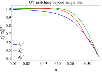
Figure 6: Ratio between the SE computed with our UV regularization procedure $S_{E}^{iw}$ with $i$ potential well and the full SE for the Coulomb potential as a function of the coupling strength $\alpha$ and fixing $v=0.02$. The blue line corresponds to the single potential well with $x_{\text{cut}}=1$, the red line corresponds to two potential wells with $x_{1}=1/6$ as defined in Eq (34). The green line shows the result with three potential wells with $x_{1}=1/3$ and $x_{2}=2/3$.

In this Appendix, we apply the procedure described in Sec. III.2 to the LO Coulomb potential where the full SE derived from wave functions defined from $(0,\infty)$ is known. In Figure 6 we show the ratio between the SE computed with the UV regularization procedure and the exact, analytical result in Eq. (6). As we can see, even for the Coulomb potential, regularizing the potential close to the origin leads to an underestimate of the SE by more than 50% at couplings close to the LO PUB.

One way to improve the precision of the calculation is to introduce more parameters to model the UV behavior of the potential. A very simple possibility is to use a series of well potentials:

$$V_{\rm reg}^{(n)}(x)=-\sum_{i}V_{i}\varphi(x_{i-1},x_{i})\ ,$$ (34)

where we defined the function $\varphi(x_{i-1},x_{i})=1$ if $x_{i-1}<x<x_{i}$ and 0 otherwise, with $x_{0}=0$ and $x_{n}=x_{\rm cut}$. Just like the single well regularization, we need to find $n$ matching conditions such to fix the potential well depths $V_{i}$. These conditions are provided by the UV scattering phases for generic angular momenta up to $l=n-1$

$$\sin\bar{\delta}_{l}=-\frac{M_{\chi}^{2}v}{2}\int_{0}^{1/M_{\chi}}\mathrm{d}rr^{2}j_{l}(kr)^{2}V(r),\quad k=\frac{M_{\chi}v}{2}\ .$$ (35)

Inside each well, the solution of the Schröedinger equation

$$-\chi_{i}^{\prime\prime}(x)+\left(\frac{l(l+1)}{x^{2}}-\frac{4V_{i}+v^{2}}{4Z_{\chi}}\right)\chi_{i}(x)=0$$ (36)

is given by the combination:

$$\chi_{i}(x)=c_{j_{l}i}\tilde{j}_{l}(\Phi_{i}x)+c_{y_{l}i}\tilde{y}_{l}(\Phi_{i}x)\ ,\quad\Phi_{i}^{2}\equiv\frac{4V_{i}+v^{2}}{4Z_{\chi}}\ ,$$ (37)

where $\tilde{j}_{l}(x)\equiv xj_{l}(x)$ $\tilde{y}_{l}(x)\equiv xy_{l}(x)$ with $j_{l}(x)$ and $y_{l}(x)$ being the regular and irregular spherical Bessel functions. The coefficients $c_{j_{l}i}$ and $c_{y_{l}i}$ are fixed by matching the solutions Eq. (37) at the boundaries of each potential well, where the coefficients $c_{j_{l}1}=1$ and $c_{y_{l}1}=0$ are determined by the boundary condition $\chi(x\rightarrow 0)\propto x^{l+1}$. The matching condition to the $l$-th scattering phase reads

$$\frac{\tilde{j}_{l}\left(\frac{vx_{\rm cut}}{2}+\bar{\delta}_{l}\right)}{\tilde{j}_{l}^{\prime}\left(\frac{vx_{\rm cut}}{2}+\bar{\delta}_{l}\right)}=\frac{v}{2\Phi_{n}}\frac{c_{j_{l}n}\tilde{j}_{l}\left(x_{\rm cut}\Phi_{n}\right)+c_{y_{l}n}\tilde{y}_{l}\left(x_{\rm cut}\Phi_{n}\right)}{c_{j_{l}n}\tilde{j}_{l}^{\prime}\left(x_{\rm cut}\Phi_{n}\right)+c_{y_{l}n}\tilde{y}_{l}^{\prime}\left(x_{\rm cut}\Phi_{n}\right)}\ ,$$ (38)

where both $c_{j_{l}n}$ and $c_{y_{l}n}$ are functions of all the $\Phi_{i}$’s. Solving the system above gives $\Phi_{i}(v,Z_{\chi})$. The wave function renormalization $Z_{\chi}$ is fixed like in the single well potential by requiring that the s-wave SE with the regularized potential is 1 at large velocities.

In Fig. 6 we the convergence of this generalized regularization procedure with the exact result for the SE for the Coulomb potential. Plotting the ratio between the approximate and the exact SE as a function of $\alpha$ we see that the agreement improves as we introduce more UV parameters.

Appendix C More about Bound States Formation

In this section, we summarize useful formulas for BSF focusing on abelian gauge theories. In Sec. C.1 we first review the basics of BSF at LO (more details can be found in Ref. [23, 11, 10, 16]). In Sec. C.2 we give a simple argument for abelian gauge theories showing the decoupling of BSF at large BS quantum numbers. In Sec. C.3 we consider NLO corrections to the BSF showing that are subleading with respect to the NLO corrections to the SE considered here. Similar results were presented in Ref. [16]. In Sec. C.4 we present a generalization of the variable phase method that we used to compute the BSF cross-sections with NLO potentials.

C.1 LO Bound States Formation

At leading order, the bound state formation proceeds in the electric dipole approximation through the emission of a single vector boson $\gamma$ as $\chi(\vec{p}_{1})+\bar{\chi}(\vec{p}_{2})\rightarrow\mathrm{BS}(\vec{q})+\gamma(\vec{k})$. This process is described by the effective Hamiltonian with the usual electric dipole term

$$\mathcal{H}^{\text{LO}}=-\frac{gq_{\chi}}{M_{\chi}}(\vec{\gamma}^{a}(x_{1})\cdot\vec{p}_{1}-\vec{\gamma}^{a}(x_{2})\cdot\vec{p}_{2})\ .$$ (39)

A BS with principal quantum number $n$, angular momentum $(l,m)$, spin $s$, labeled as ${}^{s}\mathcal{B}_{nl}$, is described by the wave function $\phi_{nlm}(r)$ satisfying the Schröedinger equation

$$-\frac{\nabla^{2}\phi_{nlm}}{M_{\chi}}+V_{i}^{\text{LO}}\phi_{nlm}=E_{nl}\phi_{nlm}\,,$$ (40)

where $E_{nl}$ is the binding energy of the BS which for a Coulomb potential is $E_{nl}=q_{\chi}^{4}\alpha^{2}M_{\chi}/4n^{2}$. The cross-section for the formation of a BS can be written as

$$\sigma_{\text{BS}}v=\!\frac{2\alpha q_{\chi}^{2}}{\pi}\frac{k}{M_{\chi}^{2}}\frac{2s+1}{g_{\chi}^{2}}\sum_{m}\int\!\!\mathrm{d}\Omega_{k}\left(|\vec{\mathcal{A}}_{p,nlm}|^{2}-\frac{|\vec{\mathcal{A}}_{p,nlm}\cdot\vec{k}|^{2}}{k^{2}+m_{\gamma}^{2}}\right),$$ (41)

where $g_{\chi}$ indicates the number of DM degrees of freedom, including those coming from internal quantum numbers and $k$ is the momentum of the emitted vector, whose mass is $m_{\gamma}$. In particular, for massless vectors $k=E_{nl}+M_{\chi}v^{2}/4$. The amplitude can be written as

$$\vec{\mathcal{A}}_{p,nlm}=\!\int\mathrm{d}^{3}r\phi_{nlm}^{*}(r)\vec{\nabla}\phi_{p}(r)\ ,$$ (42)

where we defined the scattering wave function $\phi_{p}$ satisfying Eq. (1) with $p=M_{\chi}v/2$. By inspecting the overlap integrals, we can provide a simple parametric estimate of the BSF cross-section in the $v<\alpha$ limit

$$\sigma_{\text{BS}}v\simeq\frac{8\pi^{2}\alpha q_{\chi}^{2}}{g_{\chi}^{2}M^{3}_{\chi}v}E_{nl}\ .$$ (43)

The contribution of BSF to the DM annihilation cross-section is the result of balancing three different processes in the dynamics of a BS in the plasma: i) BS annihilation into plasma states, ii) BS decay or excitation to other BSs, iii) BS ionization due to the thermal plasma.

The ionization rate in the thermal plasma can be related to the BSF cross-section in Eq. (41) through detailed balance:

$$\Gamma_{\text{break}}=\frac{g_{\chi}^{2}}{g_{\text{BS}}}\frac{(M_{\chi}T)^{\frac{3}{2}}}{16\pi^{\frac{3}{2}}}e^{-\frac{E_{nl}}{T}}\langle\sigma_{\text{BS}}v\rangle\ ,$$ (44)

and it depends exponentially on the hierarchy of thermal bath temperature $T$ and the BS binding energy $E_{nl}$. The decay/excitation rate is computed by replacing the scattering wave function in the BSF with the wave function of the excited BS. For example, in the simple dark QED model considered in Sec IV, the decay rate as a function of $n$ can be written explicitly as:

$$\Gamma_{\text{dec}}^{\text{U(1)}}\simeq\frac{(q_{\chi}^{2}\alpha)^{5}M_{\chi}}{3n^{5}}\ .$$ (45)

As shown in Ref [11, 10] the Boltzmann equations for the DM and the BS abundances can be enormously simplified whenever the rate of at least one of the three fundamental processes controlling BS dynamics is larger than the Hubble expansion. In this approximation, the effect of BSF can be encoded in an effective annihilation cross-section given by

$$\langle\sigma v\rangle=\langle\sigma_{\text{ann}}v\rangle+\sum_{\text{BS}}R_{\text{BS}}\langle\sigma_{\text{BS}}v\rangle,$$ (46)

where $R_{\text{BS}}$ is the annihilation branching ratio of the BS which for a single bound state takes a rather intuitive form $R_{\text{BS}}=\Gamma_{\text{ann}}/(\Gamma_{\text{ann}}+\Gamma_{\text{break}})$ and for a general excited state BS is

$$R_{\text{BS}}=\frac{\sum_{i}\Gamma_{\text{dec}}(\text{BS}\rightarrow\text{BS}_{i})R_{\text{BS}_{i}}}{\sum_{i}\Gamma_{\text{dec}}(\text{BS}\rightarrow\text{BS}_{i})+\Gamma_{\text{break}}}\ ,$$ (47)

assuming a negligible excitation rate. These branching ratios effectively reduce the impact of excited states on the DM abundance making the sum in Eq. (46) dominated by the BS’s with low principal quantum number $n$. In the model of Sec. IV, a very good approximation is to take $R_{\rm BS}=1$, especially at large coupling, because of the increasing Boltzmann suppression in the ionization rate. The contribution of the more excited BS, for which $R_{\rm BS}=1$ may be no longer valid, decouples very fast as we will show in Sec. C.2). We checked that the error done by neglecting all states with $n\geq 3$ is smaller than the NLO theoretical uncertainty discussed in Sec. IV.

C.2 BSF decoupling at large BS quantum number

Here we show that for abelian interactions the BSF contribution is always dominated by the formation of lowest-lying states regardless of the interactions with the plasma. First of all, for a given $n$ BSF is dominated by the formation of the state with the largest angular momentum, that is $l=n-1$. This is due to cancellations in the overlap integrals due to the oscillatory behavior of the BS radial wave function for $l<n-1$, which is absent for maximal $l$. In this latter case, in fact, the bound state wave function goes like $\phi_{n,n-1}\propto x^{n}e^{-x/n}$, where $x=r/a_{B}$ is the radial coordinate in units of the Bohr radius $a_{B}=\frac{2}{\alpha q_{\chi}^{2}M_{\chi}}$. In the large $n$ limit, we can rewrite the wave function above using the saddle point approximation

$$\phi_{n,n-1}\simeq N(n)e^{-\frac{1}{2n}\left(\frac{x}{n}-n\right)^{2}}\ ,$$ (48)

where $N(n)=n^{-11/4}$ to ensure the correct normalization of the wave function. By explicitly writing the gradient in spherical coordinates, the BSF amplitude in Eq. (41) goes like

$$\mathcal{A}_{p,n(n-1)}\simeq\int\mathrm{d}rr^{2}\phi_{p}(r)\left(\partial_{r}-\frac{n}{r}\right)\phi_{n,n-1}(r)\simeq\int\mathrm{d}rr\cos(pr)\left(\partial_{r}-\frac{n}{r}\right)\phi_{n,n-1}(r)\ ,$$ (49)

where, apart from some irrelevant phase, we took the asymptotic limit of the scattering radial wave function $\phi_{p}(r)\sim\cos(pr)/r$. At large $n$ the integral is dominated by the non-derivative term so that we can write for the BSF cross-section

$$\sigma_{\rm BS}v\propto E_{B}|\mathcal{A}_{p,n(n-1)}|^{2}\propto\left|\int\mathrm{d}r\cos(pr)\phi_{n,n-1}(r)\right|^{2}\leq\left|\int\mathrm{d}r\phi_{n,n-1}(r)\right|^{2}\ ,$$ (50)

where $E_{B}\propto 1/n^{2}$ is the BS binding energy. Plugging in the saddle point approximation of $\phi_{n,n-1}(r)$ we get

$$\sigma_{\rm BS}v\propto n^{-\frac{5}{2}}\ .$$ (51)

C.3 Additional NLO contributions

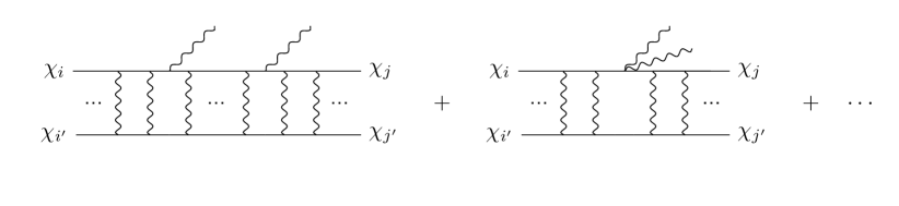
Figure 7: Examples of diagrams controlling the BS effective Hamiltonian at next-to-leading order in gauge boson emission The first diagram corresponds to the second order Born approximation for the dipole operators in (39), where the resummation of the vector boson insertions between the two emissions reconstructs the wave function of an intermediate BS or scattering state. The second diagram, instead, is obtained from the $\mathcal{O}(\gamma^{2})$ terms in the interaction Hamiltonian, at leading order in the Born approximation.

The main NLO contributions to BSF come from diagrams like the ones in Fig. 7 and are essentially of two types: i) the first diagram is essentially the second-order Born approximation of the LO Hamiltonian, with the intermediate state being a free or a BS; ii) the second diagram, where the two emitted vectors come from the same vertex, is generated by the effective Hamiltonian at order $\mathcal{O}(\gamma^{2})$. The latter contains terms of the form

$$\Delta\mathcal{H}_{I}\supset\frac{g^{2}q_{\chi}^{2}}{2M_{\chi}}\left[\vec{\gamma}\cdot\vec{\gamma}+\frac{(\vec{p}\cdot\vec{\gamma})(\vec{p}\cdot\vec{\gamma})}{M^{2}_{\chi}}\right],$$ (52)

where we focus here on the abelian part of the Hamiltonian, postponing a full study for future work. Given the above Hamiltonian, we can estimate the corresponding contribution to the double emission BSF cross-section as:

$$\Delta\sigma_{\text{BS}}v\simeq\frac{\pi}{2g_{\chi}^{2}M_{\chi}^{2}v}\left(\frac{E_{nl}}{M_{\chi}}\right)^{3}\ .$$ (53)

We now discuss the contributions from second-order Born expansion whose general expression is given by

$$(\sigma_{\rm BS}v)_{2V}=\frac{2^{6}\alpha^{2}q_{\chi}^{4}}{3^{3}g_{\chi}^{2}\pi M_{\chi}^{4}}\int\!\!\mathrm{d}\omega\omega(E_{n}-\omega)\left|\mathcal{C}_{\text{BS}}+\mathcal{C}_{\text{free}}\right|^{2}\ ,$$ (54)

where we defined

$$\mathcal{C}_{\text{BS}}=\sum_{m}\left(\frac{1}{E_{n}-E_{m}-\omega+i\Gamma_{\text{dec},m}}+\frac{1}{\omega-E_{m}+i\Gamma_{\text{dec},m}}\right)\mathcal{I}_{\vec{q}m}\mathcal{I}_{mn}\ ,$$ (55a)

$$\mathcal{C}_{\text{free}}=\int\frac{\mathrm{d}^{3}k}{(2\pi)^{3}}\left(\frac{1}{E_{n}-\omega+\frac{k^{2}}{M_{\chi}}+i\epsilon}+\frac{1}{\omega-\frac{q^{2}}{M_{\chi}}+\frac{k^{2}}{M_{\chi}}+i\epsilon}\right)\mathcal{I}_{\vec{q}\vec{k}}\mathcal{I}_{\vec{k}n}\ ,$$ (55b)

with $\mathcal{I}_{if}$ being the overlap integrals between the states $i$ and $f$, the index $m$ running over all intermediate BS and the $k$-integral running over all the intermediate scattering states.

Starting from $\mathcal{C}_{\text{BS}}$, the intermediate BS are rather narrow resonances because

$$\Gamma_{\text{dec}}\sim\alpha^{3}E_{\rm BS}\ll E_{\rm BS}\ .$$ (56)

This quick estimate, supported by the full numerical computation, suggests that $\mathcal{C}_{\text{BS}}$ contribution is fully captured in the Narrow Width Approximation (NWA) for the intermediate BS. Therefore, neglecting the interference terms, one gets

$$(\sigma_{\rm BS}v)_{2V}=\sum_{m}(\sigma_{\rm BS}v)_{1V,m}\mathrm{BR}_{m\rightarrow n}\ ,$$ (57)

which is exactly the single emission result.

To estimate the contribution from $\mathcal{C}_{\text{free}}$ we need to estimate $\mathcal{I}_{\vec{q}\vec{k}}$ which encodes the contribution from intermediate continuum states. For simplicity, we stick to the abelian contribution which reads

$$\mathcal{I}_{\vec{q}\vec{k}}=\int r^{2}\mathrm{d}rR_{\vec{k}}\partial_{r}R_{\vec{q}}\ .$$ (58)

The integral above can be split into small and large $r$ regions, roughly separated by the Bohr radius $a_{B}=\frac{1}{\alpha M_{\chi}}$

$$\begin{split}\mathcal{I}_{\vec{q}\vec{k}}=&\int_{0}^{a_{B}}r^{2}\mathrm{d}rR_{\vec{k},1}\partial_{r}R_{\vec{q}}+\int_{a_{B}}^{\infty}r^{2}\mathrm{d}rR_{\vec{k}}\partial_{r}R_{\vec{q}}\\ \sim&\frac{1}{\alpha M_{\chi}\sqrt{kq}}+\frac{q}{(M_{\chi}\alpha)^{2}}\delta(q-k)\ ,\end{split}$$ (59)

which plugged into (55) gives an estimate to $\mathcal{C}_{\text{free}}$. All in all, plugging these estimates in (54) and replacing $q=M_{\chi}v$ we get that the contribution from NLO exchange of continuum states behaves similarly to the ones estimated in (53) up to subleading terms in the $v<\alpha$ regime.

In conclusion, NLO corrections to BSF are suppressed by $\sim\alpha^{3}/64\pi$ with respect to the LO ones and can thus be neglected as compared to those considered in the main text.

C.4 Variable Phase Method for Bound State Formation

We review the Variable Phase Method (VPM) introduced in [33] (see also [34, 8, 35]) to determine the initial scattering wave function to be plugged in the overlap integrals in (42). We describe a straightforward generalization to discontinuous potentials, which allows us to compute the BSF cross-section in the presence of the regularized potential in Eq. (15).

Continuous potential.

First we review the VPM in the case of a continuous potential, assuming for simplicity a single scattering channel. This case is the case, for example, of both the LO and the NLO potentials with IR contributions in the scalar DM scenario. The generalization to multiple channels, like in the case of DM belonging to a multiplet or when spin-dependent potentials are present, like for fermionic DM, is straightforward. Consider the scattering problem described by the following Schröedinger equation

$$u^{\prime\prime}(z)+\left(1+\frac{l(l+1)}{z^{2}}\right)u(z)=\frac{4\mathcal{V}(z)}{v^{2}}u(z)\,,$$ (60)

where $u(z)=zR_{p}(z)$ is the reduced wave function and $z=M_{\chi}vr/2$ and $\mathcal{V}(z)=V(r)/M_{\chi}$. The VPM consists in writing the solution to the previous equation as a linear combination of the solutions to the free Schröedinger equation

$$\begin{pmatrix}f_{l}(z)\\ g_{l}(z)\end{pmatrix}^{\prime\prime}+\left(1+\frac{l(l+1)}{z^{2}}\right)\begin{pmatrix}f_{l}(z)\\ g_{l}(z)\end{pmatrix}=0\,,$$ (61)

where $f_{l}$ and $g_{l}$ are the regular and irregular solutions, repsectively, and are normalized as

$$f_{l}(z)g_{l}^{\prime}(z)-g_{l}(z)f_{l}^{\prime}(z)=-1\ ,$$ (62)

so that

$$f_{l}(z)=zj_{l}(z),\quad g_{l}(z)=-z(y_{L}(z)-ij_{l}(z))\,,$$ (63)

where $j_{l}$ ($y_{l}$) is the (ir)regular $l^{\text{th}}$ spherical Bessel function. We can thus write the solution to Eq. (60) as

$$u(z)=f_{l}(z)\alpha(z)-g_{l}(z)\beta(z)\,,$$ (64)

where $\alpha(z)$ and $\beta(z)$ are unknown functions. Having doubled the number of unknowns, we impose the constraint

$$f_{l}(z)\alpha^{\prime}(z)=g_{l}(z)\beta^{\prime}(z)\ .$$ (65)

Finally, in order to improve the numerical convergence, we introduce the function

$$N(z)=\left(f_{l}(z)-g_{l}(z)O(z)\right)g_{l}(z),\quad O(z)\equiv\frac{\beta(z)}{\alpha(z)}\ ,$$ (66)

so that $u=N\alpha/g_{l}$. In this way, the original second order Schröedinger equation Eq. (60) is split into two first order equations

$$N^{\prime}(z)=1+2\frac{g^{\prime}_{L}(z)}{g_{l}(z)}N(z)-\frac{4\mathcal{V}(z)}{v^{2}}N(z)^{2},$$ (67)

$$\alpha^{\prime}(z)=\frac{4\mathcal{V}(z)}{v^{2}}N(z)\alpha(z).$$

Requiring that close to the origin $u(z\rightarrow 0)=z^{l+1}/(2l+1)$ is equivalent to the following boundary conditions for $N(z)$ and $\alpha(z)$

$$N(z\rightarrow 0)=\frac{z}{2l+1},\quad\alpha(0)=(2l-1)!!\ .$$ (68)

An equivalent, numerically more stable boundary condition for $\alpha(z)$ is $\alpha(z\rightarrow\infty)=1$.

Discontinuous potential

Here we generalize the VPM method to the case of the regularized potential in Eq. (15)

$$\mathcal{V}_{\text{reg}}(x)=\left\{\begin{aligned} &-\mathcal{V}_{\rm cut}(v,x_{\text{cut}}),\quad x<x_{\rm cut}\\ &\mathcal{V}_{\text{NLO}}^{\text{UV}}(x),\qquad\quad\ \ x>x_{\rm cut}\end{aligned}\right.\ ,$$ (69)

The Schröedinger equation inside the potential well reads:

$$Z_{\chi}u^{\prime\prime}_{<}(z)+\left(1+Z_{\chi}\frac{l(l+1)}{z^{2}}\right)u_{<}(z)=-\frac{4\mathcal{V}_{\rm cut}}{v^{2}}u_{<}(z)\,.$$ (70)

In order to make the matching of $u_{<}(z)$ to the solution $u>(z)$ of the Schröedinger equation outside the well, we write:

$$u_{<}(z)=f_{l}^{<}(z)\alpha_{<}(z)-g_{l}^{<}(z)\beta_{<}(z)\,,$$ (71)

where $f_{l}^{<}(z)$ and $g_{l}^{<}(z)$ solve

$$Z_{\chi}\begin{pmatrix}f_{l}^{<}(z)\\ g_{l}^{<}(z)\end{pmatrix}^{\prime\prime}+\left(1+Z_{\chi}\frac{l(l+1)}{z^{2}}\right)\begin{pmatrix}f_{l}^{<}(z)\\ g_{l}^{<}(z)\end{pmatrix}=0\ .$$ (72)

We keep the same normalization and constraint as in Eq. (62) and Eq. (65), so that

$$f_{l}^{<}(z)=Z_{\chi}^{\frac{1}{4}}zj_{l}\left(\frac{z}{\sqrt{Z_{\chi}}}\right),\quad g_{l}^{<}(z)=-Z_{\chi}^{\frac{1}{4}}z\left(y_{l}\left(\frac{z}{\sqrt{Z_{\chi}}}\right)-ij_{l}\left(\frac{z}{\sqrt{Z_{\chi}}}\right)\right)\ .$$ (73)

Equivalently to the continuous case, we define the function $N_{<}$ inside the well as

$$N_{<}(z)=\left(f^{<}_{L}(z)-g^{<}_{L}(z)O_{<}(z)\right)g^{<}_{L}(z),\quad O_{<}(z)\equiv\frac{\beta_{<}(z)}{\alpha_{<}(z)}\,,$$ (74)

where now $N_{<}$ and $\alpha_{<}$ solve

$$N^{\prime}_{<}(z)=1+2\frac{g^{\prime<}_{L}(z)}{g^{<}_{L}(z)}N_{<}(z)+\frac{4\mathcal{V}_{\rm cut}}{Z_{\chi}v^{2}}N^{2}_{<}(z)\ ,$$ (75)

$$\alpha^{\prime}_{<}(z)=-\frac{4\mathcal{V}_{\rm cut}}{Z_{\chi}v^{2}}N_{<}(z)\alpha_{<}(z)\ .$$

The matching of $N_{<}$ and $\alpha_{<}$ to the corresponding functions defined outside the well, $N_{>}$ and $\alpha_{>}$ is obtained by requiring the continuity of $u(z)$ and $u^{\prime}(z)$ accross the boundary of the well itself. This leads to

$$O_{>}=\left.\frac{f_{l}f^{\prime<}_{L}-f_{l}^{\prime}f_{l}^{<}+O_{<}(g_{l}^{<}f_{l}^{\prime}-g^{\prime<}_{L}f_{l})}{g_{l}f^{\prime<}_{L}-g_{l}^{\prime}g_{l}^{<}+O_{<}(g_{l}^{<}g_{l}^{\prime}-g^{\prime<}_{L}<g_{l})}\right|_{z=vx_{\rm cut}/2}\ ,$$ (76)

where $f_{l}$ and $g_{l}$ are defined in Eq. (63) while $O_{<}(vx_{\rm cut}/2)$ is determined solving the equation for $N_{<}$ with initial condition $N_{<}(z\rightarrow 0)=z^{l+1}/(2l+1)$. Finally, the matching of $\alpha_{<}$ is simply

$$\left.\frac{N_{<}\alpha_{<}}{g_{l}^{<}}\right|_{z=vx_{\rm cut}/2}=\left.\frac{N_{>}\alpha_{>}}{g_{l}}\right|_{z=vx_{\rm cut}/2}\ ,$$ (77)

where $\alpha_{>}$ solves Eq. (67) with the same boundary condition $\alpha_{>}(z\rightarrow\infty)=1$.