The Planetary Accretion Shock. III.
Smoothing-free 2.5D simulations and calculation of H $\alpha$ emission

Abstract

Surveys have looked for H $\alpha$ emission from accreting gas giants but found very few objects. Analyses of the detections and non-detections have assumed that the entire gas flow feeding the planet is in radial free-fall. However, hydrodynamical simulations suggest that this is far from reality. We calculate the H $\alpha$ emission from multidimensional accretion onto a gas giant, following the gas flow from Hill-sphere scales down to the circumplanetary disc (CPD) and the planetary surface. We perform azimuthally-symmetric radiation-hydrodynamics simulations around the planet and use modern tabulated gas and dust opacities. Crucially, contrasting with most previous simulations, we do not smooth the gravitational potential and do follow the flow down to the planetary surface, where grid cells are 0.01 Jupiter radii small radially. We find that only roughly one percent of the net gas inflow into the Hill sphere reaches directly the planet. As expected for ballistic infall trajectories, most of the gas falls at too large a distance on the CPD to generate H $\alpha$. Including radiation transport removes the high-velocity sub-surface flow previously seen in hydrodynamics-only simulations, so that only the free planet surface and the inner regions of the CPD emit substantially H $\alpha$. Unless magnetospheric accretion, which we neglect here, additionally produces H $\alpha$, the corresponding H $\alpha$ production efficiency is much smaller than usually assumed, which needs to be taken into account when analysing (non-)detection statistics.

2023 July 19

1 Introduction

Over the last roughly three percent of a millennium, hundreds of extrasolar super-Jupiters have been discovered (Zhu & Dong, 2021). However, only very few of those objects are young ($\lesssim 100$ Myr). These are accessible almost only at large separations from their host star, through direct imaging ($\sim 10$–$100$ au; Wagner et al., 2019; Vigan et al., 2021, e.g.,). A few more are predicted to be on the verge of being discovered (Asensio-Torres et al., 2021) but this would not change the overall abundance qualitatively. Despite dedicated surveys (Cugno et al., 2019; Zurlo et al., 2020; Xie et al., 2020; Follette et al., 2023; Huélamo et al., 2022), fewer gas giants yet have been caught accreting. It is a robust theoretical prediction that gas undergoing a shock at velocity $v_{0}$ above a critical value, $v_{0}>{v_{\textrm{H}\,\alpha,\,\textrm{crit}}}\approx 30~{}\textrm{km}\,\textrm{s}^{-1}$, will emit hydrogen lines as the hydrogen ionised by the shock recombines and cools in the geometrically thin postshock region (Aoyama et al., 2018, 2020). There are only a few planetary-mass companions with observed line emission clearly linked to a shock: PDS 70 b and c (Wagner et al., 2018; Haffert et al., 2019) at H $\alpha$, and Delorme 1 (AB)b at several lines (Eriksson et al., 2020; Betti et al., 2022a, b; Ringqvist et al., 2023). However, only the PDS 70 planets are found in a gas disc, and the others are effectively isolated. At newly-discovered AB Aur b, point-like H $\alpha$ emission is observed but scattering of stellar photons cannot be excluded as the source (Currie et al., 2022; Zhou et al., 2022).

Different factors can explain the scarcity of H $\alpha$-emitting accreting planets detected at large separations. Most planets are possibly forming closer in to their star, as classically expected from core accretion (e.g., Thommes et al., 2008; see also review in Emsenhuber et al., 2021) and thus inside the inner working angle (IWA) of current-generation detectors (Close, 2020). Planets could also be accreting episodically, with only brief and therefore unlikely-to-be-caught periods of detectably high accretion (e.g., Brittain et al., 2020). Another possibility is that the H $\alpha$ and the other hydrogen lines are absorbed by the protoplanetary disc (PPD). Since massive planets open a deep gap in the gas and dust distributions, this might not be an important effect. As an example, scaling the simulations of Sanchis et al. (2020) to the PDS 70 system, extinction by the PPD is negligible for their specific accretion rate (see discussion in Section 7.6 of Marleau et al. 2022). Alternatively, the gas and dust flowing onto the planet could absorb the H $\alpha$, but Marleau et al. (2022) estimated this not to be important for most planet accretion rates and masses.

Two more factors are of particular importance yet underappreciated. One is that line emission in the planetary-mass regime, especially in the absence of magnetospheric accretion, is intrinsically weaker than for stars for a given mass infall rate (Aoyama et al., 2021).

The second factor is that most of the infalling and supersonic gas likely does not reach the planet directly but rather shocks onto a circumplanetary disc (CPD) at a significant fraction of the Hill radius ${R_{\textrm{Hill}}}$ away from the planet. This consequence of angular momentum conservation holds for matter inflowing due only to the action of gravity (i.e., ballistically; Mendoza et al., 2009). In the planet formation context, it was pointed out by Tanigawa et al. (2012), who found in their isothermal hydrodynamical simulations that the gas hitting the CPD around a Jupiter-mass planet was spread uniformly over a region of size $\sim 0.1~{}{R_{\textrm{Hill}}}\sim 100~{}R_{\textrm{J}}$. This shock should heat up the CPD and possibly make it detectable in the near infrared (Szulágyi et al., 2019). However, for typical planet masses the velocity of the gas at the shock $v_{0}\sim 1/\sqrt{r}$ (see Equation (2) below) is too low at large distances for significant line emission from the shock (i.e., it has $v_{0}<{v_{\textrm{H}\,\alpha,\,\textrm{crit}}}$). This implies that only the small fraction of the mass inflow that hits the planetary surface and the innermost region of the CPD would be responsible for line emission. These regions were however not resolved in their simulations. Similarly, other recent work addressing H $\alpha$ generation is limited in different ways, as we review in Section 2.

In this work, we study mass infall onto the planetary surface and the CPD, including its innermost regions. To enable an appropriately high resolution $\Delta r\ll R_{\textrm{J}}$, we make the compromise of a simplified dimensionality but otherwise use methods matching or improving previous studies. We then predict the H $\alpha$ emission using detailed shock emission models designed for the planetary regime.

This paper is structured as follows. Section 2 summarises related studies in the literature and Section 3 presents our physical model and numerical methods. In Section 4 we discuss the properties of the flow, estimate the amount of generated H $\alpha$, and assess the effect of varying some input parameters. In Section 5, we compare our results to previous work before presenting a more general discussion. Finally, in Section 6 we summarise our findings and conclude.

2 Previous studies of accreting planets

Table 1: Comparison of some (radiation-)hydrodynamical studies of accreting gas giants.

H $\alpha$	Study and Dimensionality		Domain size	Thermodynamics	Smoothing ${\varepsilon_{\textrm{grav}}}$	Resolution $\Delta r$
	Machida et al. (2008)	3D	$(30,~{}120,~{}8)~{}{H_{P}}$	isothermal	0.0060 ${H_{P}}$	0.0070 ${H_{P}}$
	Tanigawa et al. (2012)	3D	$(24,~{}24,~{}6)~{}{H_{P}}$	isothermal	0.0007 ${H_{P}}$	0.0004 ${H_{P}}$
	Béthune & Rafikov (2019b)	3D	128 $R_{\textrm{p}}$	isothermal	none	0.1 RJ
	Fung et al. (2019)	3D	global	isothermal	0.05 ${H_{P}}$	0.02 ${R_{\textrm{Hill}}}$
*	Szulágyi & Ercolano (2020)	3D	global	FLD	20 $R_{\textrm{J}}$	0.9 $R_{\textrm{J}}$
	Dong et al. (2021)	2.5D	10 $R_{\textrm{p}}$	isothermal	none	0.001 Rp
*	Takasao et al. (2021)	2.5D	$0.03~{}{R_{\textrm{Hill}}}\approx 100~{}R_{\textrm{p}}$	$\gamma=1.01,\,1.05$	none	0.005 Rp
	Maeda et al. (2022)	3D	$(24,~{}24,~{}6)~{}{H_{P}}$	isothermal	0.0002 ${H_{P}}$	0.0004 ${H_{P}}$
*	This work	2.5D	$1~{}{R_{\textrm{Hill}}}\approx 4100~{}R_{\textrm{J}}$	FLD	none	0.001 RJ

Note. — Particularly commendable settings are highlighted in bold. All simulations reported here are for gas giants and/or have ${q_{\textrm{th}}}\gtrsim 2$ (see Section 3.3 for this parameter and others mentioned here). Dong et al. (2021) is included for comparison even though they do not allow infall from the outer edge. We take the case ${q_{\textrm{th}}}=4$ of Béthune & Rafikov (2019b) and Fung et al. (2019), $M_{\textrm{p}}=3~{}M_{\textrm{J}}$ of Szulágyi & Ercolano (2020), and ${R_{\textrm{Hill}}}/{H_{P}}=1.36$ (${q_{\textrm{th}}}=7.5$) of Maeda et al. (2022) because they are closest to our fiducial values (Table 2).

Previous studies have looked at the accretion flow toward a forming planet. Pioneering work was presented by Ayliffe & Bate (2009a, b, 2012). However, most investigations (e.g., those and Cimerman et al., 2017; Kurokawa & Tanigawa, 2018; Béthune & Rafikov, 2019b; Schulik et al., 2019, 2020; Mai et al., 2020; Bailey et al., 2021; Moldenhauer et al., 2021; Krapp et al., 2022; Moldenhauer et al., 2022) were concerned with low planet masses (super-Earths to at most $1~{}M_{\textrm{J}}$), for which no H $\alpha$ from an accretion shock can be expected because the infall velocity is too low (see Equation (2); Aoyama et al., 2018). The few works exploring accretion onto gas giants have limited spatial resolution ($\Delta r\sim R_{\textrm{J}}$) and, most problematically, a sizeable gravitational potential smoothing length ${\varepsilon_{\textrm{grav}}}\sim 10~{}R_{\textrm{J}}$ or larger, which even modern computational resources impose (e.g., Machida et al., 2008; Tanigawa et al., 2012; Szulágyi, 2017; Lambrechts et al., 2019; Fung et al., 2019; Szulágyi & Ercolano, 2020). Table 1 provides an overview. This significant ${\varepsilon_{\textrm{grav}}}$ affects the flow already on scales of a few times ${\varepsilon_{\textrm{grav}}}$ (i.e, out to roughly $r\sim 30~{}R_{\textrm{J}}$ to 100 $R_{\textrm{J}}$ or more) by weakening the effective mass of the planet. This could thus change qualitatively the flow pattern at the length scales that set the shock velocity, which is a sensitive factor for the H $\alpha$ emission. In Table 1, studies predicting H $\alpha$ emission are highlighted by an asterisk (*).

A notable exception to the issue of a large smoothing of the gravitational potential is the work of Takasao et al. (2021), who consider the full potential (${\varepsilon_{\textrm{grav}}}=0$) of their 12-$M_{\textrm{J}}$ planet. Their cell size $\Delta r\sim 0.01~{}R_{\textrm{J}}$ close to the planet is also adequate to resolve the flow details. However, they do not include radiation transfer and adopt a heat capacity ratio $\gamma=1.01$ or $\gamma=1.05$. We will compare with their work in Section 5.2 and find crucial differences in the post-shock structures and thus in the emission of H $\alpha$. Therefore, including radiation transfer while setting ${\varepsilon_{\textrm{grav}}}=0$ seems desirable for more realistic simulations.

In this work, we complement the studies in the literature by considering the full, non-smoothed potential with a high spatial resolution while including radiation transport. As a compromise, instead of resolving the 3D structure of the flow, we assume axisymmetry around the planet. We describe our model in detail in the next section.

3 Physical model and numerical methods

3.1 Approach: Local simulations in 2.5D

We consider a super-Jupiter forming by runaway accretion in a PPD and study the flow around the planet from Hill-sphere scales down to length scales much smaller than a Jupiter radius. The dynamical timescales near the planet are much shorter than the dynamical or even viscous timescales of the PPD. Therefore, we do not evolve the background PPD and take it as a fixed boundary condition, assuming a circular orbit for the planet. We expect the flow around the planet to reach a quasi-steady state over a few free-fall times from the Hill sphere down to the planetary surface. While this is not a true steady state because of accretion, this state may represent an instantaneous snapshot in the accretion history of the planet. We also assume that a quasi-steady state is reached much faster than the mass or accretion rate of the planet change while it forms.

Initially, the domain contains a negligible amount of mass and thermal energy (see Section 3.2.4). However, there is no well-defined final amount of mass and thermal energy because the quasi-steady state is an essentially constant accretion flow ($d\dot{M}/dt\sim 0$), not the absence of accretion ($\dot{M}\sim 0$). Consequently, we do not attempt to predict quantities such as the CPD thickness, size, or temperature, or the interior luminosity of the accreting planet. They will likely depend on the simulation history, which is not guaranteed to be equivalent to a global calculation of planet formation in an evolving PPD. Instead, quantities such as the CPD thickness or planet luminosity should be seen as independent parameters that can be measured in the simulation results. They change slowly in the quasi-steady state.

The physical domain of our simulations extends to the Hill sphere. This is a compromise between, on the one hand, simulating the whole PPD structure, which would be computationally expensive but also sensitive to several poorly-constrained modelling choices (e.g., strength and spatial dependence of viscosity, presence of disc winds, dust grain size evolution and feedback on the gas), and, on the other hand, considering a region only several planetary radii large, which would let the chosen boundary conditions at that location determine too strongly the gas flow. Our assumption of axisymmetry around the planet will break down significantly further away than the Hill sphere, where the star’s gravity dominates. Therefore, simulating out to ${R_{\textrm{Hill}}}$ is a natural choice.

This paper extends to a more realistic geometry our previous work in this series (Marleau et al., 2017, 2019; hereafter Paper I and Paper II), in which we simulated and analysed the properties of the accretion flow and the accretion shock with highly-resolved 1D models for purely radial infall. The emphasis in the present work is on the flow geometry when including angular momentum conservation.

3.2 Numerical methods

To solve the radiation-hydrodynamics, we use the open-source (magneto)hydrodynamics code Pluto (Mignone et al., 2007, 2012) in combination with the radiation transport package Makemake (Kuiper et al., 2020). The Courant–Friedrichs–Lewy number is kept at $\textrm{CFL}=0.4$, except for the simulation of Section 4.4, which uses $\textrm{CFL}=0.33$. We use the non-equilibrium (two-temperature) flux-limited diffusion (FLD) module (Kuiper et al., 2010, 2020) as in Paper I and Paper II. As argued in Tanigawa et al. (2012), we do not include viscosity since we study the supersonic flow, not the CPD structure. Also, self-gravity is negligible. Makemake has been extensively tested and used in a variety of contexts (see Kuiper et al. 2020 and references thereto).

We do not set floor values on quantities such as the density or pressure. The only exception is a minimum on the radiation temperature ${T_{\textrm{rad}}}=({E_{\textrm{rad}}}/a_{\textrm{r}})^{1/4}\sim 10^{-10}$ K (where $a_{\textrm{r}}$ is the radiation constant) during the numerical iterations to solve the FLD equation system to prevent ${E_{\textrm{rad}}}\leqslant 0$ K from ever being reached. The smallest temperatures in the converged profiles are however much higher ($T\gtrsim 10$ K), as expected.

3.2.1 Coordinate system, domain size, forces, and resolution

We consider a simulation region in the $r$–$\theta$ (poloidal, or vertical) plane centred on the planet and averaged over $\phi$, where $r$, $\theta$, and $\phi$ are the usual radial, spherical polar (co-latitudinal), and azimuthal coordinates. We simulate the upper hemisphere and assume symmetry at the midplane ($\theta=90$°). The radial grid ranges from ${r_{\textrm{min}}}=1.9~{}R_{\textrm{J}}$ to ${r_{\textrm{max}}}$, with ${r_{\textrm{max}}}$ a near-unity factor of ${R_{\textrm{Hill}}}$. Our fiducial simulation has ${r_{\textrm{max}}}={R_{\textrm{Hill}}}$. With ${r_{\textrm{min}}}=1.9~{}R_{\textrm{J}}$, the shock that defines the planet surface is usually at $R_{\textrm{p}}\approx 2~{}R_{\textrm{J}}$, changing only slowly during the simulation. This commonly-used size is thought to be appropriate for forming or young planets (Marley et al., 2007; Mordasini et al., 2012a; Zhu, 2015).

We include the gravity of the planet by adding a radial acceleration $g=-GM_{\textrm{p}}/r^{2}$ everywhere, where $M_{\textrm{p}}$ is the constant mass of the planet. Thus we avoid any smoothing and set ${\varepsilon_{\textrm{grav}}}=0$. Since the mass in the whole simulation domain is always negligible, no self-gravity is needed. We do not include the vertical component of the star’s gravity directly in the simulation. Above the planet, it would dominate over the planet’s gravity for $z\gtrsim 3^{(1/3)}{R_{\textrm{Hill}}}$, making the star’s gravity only a small correction to the dynamics in the region we simulate. However, we do impose the appropriate density stratification at the outer edge of the domain, which is sufficient (see Equation (1) below).

We follow the azimuthal component of the velocity $v_{\phi}$ despite the azimuthal symmetry, making the simulation 2.5D. The simulations include the Coriolis and centrifugal terms due to the planet’s Keplerian orbit around the star. This is done in a linearised, conservative form (Kley, 1998) by enabling the ROTATING_FRAME option of Pluto.

We use a very fine radial gridding close to the inner edge with $\Delta r=10^{-3}~{}R_{\textrm{J}}$, where the atmosphere is in rotation-modified hydrostatic equilibrium. The cell size increases smoothly outwards. Near the shock that terminates the atmosphere and defines the radius of the planet, cells have $\Delta r\sim 10^{-2}~{}R_{\textrm{J}}$. Beyond $r\approx 2.5~{}R_{\textrm{J}}$, the cell size increases logarithmically with 76 cells per decade, reaching $\Delta r\approx 100~{}R_{\textrm{J}}$ at ${R_{\textrm{Hill}}}$. Appendix A gives further details.

The standard polar grid is uniform with ${N_{\theta}}=181$ cells from pole to equator ($\Delta\theta\approx 0.5$°). Simulations with ${N_{\theta}}=91$ and even ${N_{\theta}}=51$ ($\Delta\theta\approx 1.8$°) yielded the same results overall. The only difference is that only in the middle- and high-resolution simulations is a thin supersonic flow beneath the surface of the CPD visible. We discuss this in Appendix B.

3.2.2 Boundary conditions

The radial boundary conditions are described in the next two sections. In the polar ($\theta$) direction, we use reflective and equatorially symmetric boundary conditions at the pole and midplane, respectively.

Boundary conditions at the outer edge

We assume the surrounding PPD to be vertically isothermal and in hydrostatic equilibrium. We do not include the stellar potential, but we fix the density at the outer edge to

$$\rho({r_{\textrm{max}}},\theta)={\rho_{\textrm{mid}}}\exp\left[-0.5\left(\frac{z}{{H_{P}}}\right)^{2}\right],$$ (1)

where $z=r\cos\theta$ is the height above the midplane, and ${\rho_{\textrm{mid}}}=\Sigma/(\sqrt{2\pi}{H_{P}})$ is the midplane volume density in the gap with constant surface density $\Sigma$ (see below Expression (7)). Equation (1) thus correctly mimics the influence of the central star.

The poloidal components of the velocity are set as follows at ${r_{\textrm{max}}}$. We set $v_{\theta}=0$. The radial velocity has $dv_{r}/dr=0$ to allow both inflow ($v_{r}<0$) and outflow ($v_{r}>0$) but it is limited in magnitude on the negative side to the freefall velocity from infinity,

$${v_{\textrm{ff},\,\infty}}(r)=\sqrt{\frac{2GM_{\textrm{p}}}{r}}=60~{}\textrm{km}\,\textrm{s}^{-1}\sqrt{\frac{M_{\textrm{p}}/2~{}M_{\textrm{J}}}{r/2~{}R_{\textrm{J}}}}.$$ (2)

Locally in the rotating frame, the flow of the PPD reduces to a simple linear shear (Hill, 1878; Goldreich & Lynden-Bell, 1965), which we average along $\phi$ to obtain the azimuthal component of the velocity. Taking $x$ to point away from the star along the star–planet direction and $y$ along the orbit of the planet, the shear is $v_{y}=-q\Omega_{0}x$, where the Keplerian orbital angular frequency of the planet is $\Omega_{0}=\sqrt{G{M_{\star}}/a^{3}}$ for a semi-major axis $a$, and $q=3/2$ for a Keplerian potential. Since $x=R\sin\phi$, with $R$ the cylindrical radius, we have $v_{\phi}=-q\Omega_{0}R\sin^{2}\phi$, with a $\phi$ average $\langle v_{\phi}\rangle=-\frac{1}{2}q\Omega_{0}R$. We therefore set

$$v_{\phi}({r_{\textrm{max}}})=\langle v_{\phi}\rangle=-\frac{3}{4}\Omega_{0}{r_{\textrm{max}}}\sin\theta.$$ (3)

This is an approximation since a shear flow is an exact description of the motion of the gas only close to the planet while neglecting its presence at the same time.

Averaging the same way the radial component gives $\langle v_{r}\rangle=0$, which we obviously do not use for $v_{r}$ because it would prevent accretion into the domain. In reality, due to the planet’s gravity there is no pure shear flow but rather complex horseshoe orbits with “U-turns” and other features that can be captured only in 3D (e.g., Tanigawa et al., 2012; Schulik et al., 2020). Thus, setting $dv_{r}/dr=0$ as detailed above is a simple attempt to circumvent the limitation of a formally-averaged 2.5D approach.

Finally, we take a zero-gradient boundary condition for the gas pressure ($dP/dr=0$), which however is unimportant because the gas is supersonic for ${r_{\textrm{max}}}<{R_{\textrm{Bondi}}}$, which will hold for our cases of interest. We set $d(r^{2}{E_{\textrm{rad}}})/dr=0$ for the radiation energy density ${E_{\textrm{rad}}}$; if the radiation is free-streaming at ${r_{\textrm{max}}}$ (as it does turn out to be), this corresponds to a zero-gradient condition on the luminosity (Paper I).

Boundary conditions at the inner edge

Young planets have been observed to spin at 5 % to 20 % of their break-up frequency (e.g., Bryan et al., 2018, 2020). Therefore we let the planet rotate at ${r_{\textrm{min}}}$ as a solid body by setting $v_{\phi}(\theta)={f_{\omega}}{\omega_{\textrm{crit}}}{r_{\textrm{min}}}\sin\theta$, where the critical or break-up frequency is given by (see e.g. Section 4 of Paxton et al. 2019)

$${\omega_{\textrm{crit}}}\approx\sqrt{\frac{GM_{\textrm{p}}}{R_{\textrm{p}}^{3}}},$$ (4)

with the normalised spin ${f_{\omega}}$ set to 0.1. Planets spinning at near-break-up rates (${f_{\omega}}\approx 0.8$) might shed mass more than accrete (Dong et al., 2021; Fu et al., 2023) but smaller values should not influence significantly the transport of either mass or momentum in the CPD, and certainly not in the supersonic part of the flow. Therefore, we do not vary ${f_{\omega}}$.

As in Paper I and Paper II, the inner edge is closed, without flow of matter. Therefore, we set $d\rho/dr=0$ at ${r_{\textrm{min}}}$ and use a reflecting condition on the radial velocity: $v_{r}({r_{\textrm{min}}}^{-})=-v_{r}({r_{\textrm{min}}}^{+})$, where ${r_{\textrm{min}}}^{+\,(-)}$ is above (below) ${r_{\textrm{min}}}$. This lets an atmosphere in equilibrium build up beneath the settling zone. We use a no-slip boundary condition: $v_{\theta}=0$. The pressure is determined by hydrostatic equilibrium in the presence of rotation:

$$\frac{dP}{dr}=-\rho\left(g-\frac{v_{\phi}^{2}}{r}\right),$$ (5)

where $g=-GM_{\textrm{p}}/r^{2}$ (see above).

At the inner edge, we choose a small luminosity $L({r_{\textrm{min}}})=10^{-7}~{}{L_{\odot}}$ and impose accordingly across the interface $d{E_{\textrm{rad}}}/dr=L/(4\pi r^{2})/D_{\textrm{F}}$, where $D_{\textrm{F}}=\lambda c/({\kappa_{\textrm{R}}}\rho)$ is the local diffusion coefficient, with $\lambda$ the flux limiter (see details in Paper I) and ${\kappa_{\textrm{R}}}$ the Rosseland mean opacity. The luminosity increases outwards due to the compression of the accreting gas (Paper II).

3.2.3 Microphysics

As in our previous work, Rosseland- and Planck-mean opacities are taken from Malygin et al. (2014) for the gas, and from Semenov et al. (2003, model nrm_h_s) for the dust, with the dust sublimation as in Isella & Natta (2005). The maximal dust-to-gas mass ratio is $f_{\textrm{d/g}}=10^{-4}$. This reduction with respect to the ISM value reflects the fact that the “pressure bump” induced by the planet in the PPD could keep out opacity-carrying grains from the gap (Drążkowska et al., 2019; Chachan et al., 2021; Karlin et al., 2023; but see Szulágyi et al., 2022). This is however uncertain and $f_{\textrm{d/g}}$ could be varied in future work.

For the equation of state (EOS), we use a perfect gas with a constant mean molecular weight $\mu=2.3$ and adiabatic index $\gamma=1.4$, appropriate for a solar mixture of H₂ and He with a hydrogen mass fraction $X=0.75$. In Paper I and Paper II we have shown that the choice of $\mu$ and $\gamma$ does not affect the hydrodynamic structure of the accretion flow (as seen also in Chen & Bai 2022). The CPD properties, in particular its thickness, might be affected especially by $\mu$ but the accretion history is likely as important a factor. We recall that we do not wish to predict quantitative properties of the CPD here. Thus the choice of the EOS will not bear qualitatively on the results.

3.2.4 Reaching quasi-steady state

Gas is free to flow into the simulation domain from the outer edge. For a steady state to be reached, at least a few global free-fall times need to elapse. Evaluating at $r={r_{\textrm{max}}}$ the free-fall time from any radius $r$ to a much smaller position (e.g., Mungan, 2009) yields the global free-fall time

$${t_{\textrm{ff,\,glob}}}=\pi\sqrt{\frac{{r_{\textrm{max}}}^{3}}{8GM_{\textrm{p}}}}.$$ (6)

By definition of free-fall, Equation (6) ignores angular momentum. In reality, the latter will reduce the radial velocity of the gas and thus increase its fall time. For reference, if ${r_{\textrm{max}}}$ is always set to ${R_{\textrm{Hill}}}$, the free-fall time becomes ${t_{\textrm{ff,\,glob}}}=(2\pi/\Omega_{0})/\sqrt{96}$ or one tenth of an orbital period.

We initialise the simulation with small density and temperature values that decrease outward independently of angle, and set ${T_{\textrm{rad}}}=T$ (where $T$ is the gas temperature), $v_{r}=v_{\theta}=0$, and $v_{\phi}=-0.75\Omega_{0}R$ throughout. This state is quickly “forgotten” over a timescale comparable to ${t_{\textrm{ff,\,glob}}}$ as the gas begins to fall due to gravity of the planet. The accreting gas accumulates in a CPD whose outer edge is defined by a radial shock and grows slowly over time.

To speed up the computation, we use two phases. In Phase I, while we let the large-scale and supersonic flow reach a quasi-steady state that erases the initial conditions, we do not compute the hydrodynamics of the innermost region, whose early-time properties will be unimportant once the gas from ${r_{\textrm{max}}}$ reaches it. We use Pluto’s FLAG_INTERNAL_BOUNDARY to make inactive the cells between ${r_{\textrm{min}}}$ and a “freeze radius” set to ${r_{\textrm{frz}}}=10~{}R_{\textrm{J}}$. Importantly, the inactive cells are ignored when determining the hydrodynamics timestep $\Delta t$. From the Courant condition, $\Delta t$ increases with cell size and decreases with temperature. Therefore, not having to take the innermost cells into account, which are the smallest (Figure 8) and the hottest (Figure 10), speeds up computations considerably. The radiation transport is always solved over the full domain, both in Phase I and the subsequent Phase II (described next).

After a few global free-fall times in Phase I, we restart the simulation but now evolve the density and velocity everywhere as usual. This is Phase II. After a brief transition period, no features remain at ${r_{\textrm{frz}}}$ and all quantities $(\rho,v,P,{T_{\textrm{rad}}})$ are smooth. We run Phase II for thousands of free-fall times from ${r_{\textrm{frz}}}$ (numerical details are given in Section 3.4). By Equation (6), the free-fall time at ${r_{\textrm{frz}}}$ down to “$r=0$” is roughly ${t_{\textrm{ff,\,frz}}}=({r_{\textrm{frz}}}/{R_{\textrm{Hill}}})^{1.5}{t_{\textrm{ff,\,glob}}}\approx{t_{\textrm{ff,\,glob}}}/8000$. Thus, over the course of Phase II the inner regions are in quasi-steady state given the large-scale flow, while the large-scale flow cannot change appreciably since Phase II lasts for $\lesssim{t_{\textrm{ff,\,glob}}}$.

A feature of our set-up is that the CPD has to build up from the infalling gas since we do not put in any structure initially. The accreting gas naturally accumulates in a CPD whose outer edge is defined by a radial shock and increases over timescales of hundreds of ${t_{\textrm{ff,\,glob}}}$. The thickness (the aspect ratio) of the CPD does not vary much while it grows. The formation of the CPD causes a spherical shock to propagate outward through the infalling material, with part of shock at the position of the expanding outer edge of the CPD. Consequently, the flow pattern close to the planet is not quite in steady state. We estimate in Appendix C how much this affects our analysis and find that it should not change our conclusions. Therefore, for simplicity we will call the Phase II state with a qualitatively constant flow pattern a quasi-steady state, and analyse this, keeping in mind that over much longer timescales there are likely quantitative fluctuations.

3.3 Free parameters

One can parametrise the degrees of freedom of the problem in different ways. To help bridge simulations and observations, we choose as independent parameters

$$\left({M_{\star}},a,\Sigma,h,{r_{\textrm{max}}},M_{\textrm{p}},R_{\textrm{p}}\right),$$ (7)

where, repeating some definitions, ${M_{\star}}$ is the stellar mass, $a$ the semi-major axis of the planet, $\Sigma$ the PPD surface density at $a$ as reduced by gap opening, $h$ the PPD aspect ratio at $a$, $M_{\textrm{p}}$ the planet mass, and $R_{\textrm{p}}$ the physical radius of the planet. Instead of setting $\Sigma$ directly, one could choose a value for the viscosity parameter $\alpha$ (Shakura & Sunyaev, 1973) and an unperturbed surface density of the PPD $\Sigma_{0}$, and, following Kanagawa et al. (2018), let $\Sigma=\Sigma_{0}/(1+K/25)$, where $K=q^{2}/(\alpha h^{5})$.

To be consistent with the approximation of symmetry around the planet, one should choose ${r_{\textrm{max}}}$ to be smaller than the width of the gap, which we do not model. This choice also predicts the reduced surface density to be constant across the gap (Kanagawa et al., 2017), which we assume when setting $\rho({r_{\textrm{max}}})$ (Equation (1)). Also, we introduced the parameter ${r_{\textrm{max}}}$ because we do not simulate the whole PPD. However, ${r_{\textrm{max}}}$ should be seen primarily not as a numerical parameter but rather as a (simple) way of controlling the incoming angular momentum of the gas. We vary ${r_{\textrm{max}}}$ in Section 4.3.

The other characteristic quantities follow from Expression (7): the planet–star mass ratio $q=M_{\textrm{p}}/{M_{\star}}$; the Hill radius ${R_{\textrm{Hill}}}=a\left(M_{\textrm{p}}/[3{M_{\star}}]\right)^{1/3}$; the Bondi radius ${R_{\textrm{Bondi}}}=aq/h^{2}$; the pressure scale height ${H_{P}}=ah$; the Keplerian orbital angular frequency of the planet $\Omega_{0}$ (defined above Equation (3)); and in particular ${q_{\textrm{th}}}$, the ratio between the planet mass and the “disc thermal mass” (for short, “the thermal mass”; e.g., Korycansky & Papaloizou, 1996; Machida et al., 2008; Fung et al., 2019):

$${q_{\textrm{th}}}=q/h^{3}={R_{\textrm{Bondi}}}/{H_{P}}=3({R_{\textrm{Hill}}}/{H_{P}})^{3}.$$ (8)

When $R_{\textrm{p}}\ll\min({R_{\textrm{Bondi}}},{R_{\textrm{Hill}}})$, in the isothermal and inviscid limit, one may expect ${q_{\textrm{th}}}$ to be the only parameter controlling the flow in a local region around a planet on a Keplerian orbit (Korycansky & Papaloizou, 1996; see however Béthune & Rafikov, 2019a, b). The radiation transfer introduces a physical scale through the temperature- and density-dependent opacities, but qualitatively ${q_{\textrm{th}}}$ should be key in determining the flow.

One characteristic quantity emerges from our set-up: the net mass inflow rate into the Hill sphere $\dot{M}_{\textrm{Hill,\,net}}$, that is, what flows in minus what flows out. This in turn is set by more global PPD physics (e.g., Nelson et al., 2023; Choksi et al., 2023). The growth rate of the planet cannot be controlled directly but is at most $\dot{M}_{\textrm{Hill,\,net}}$; it is less if some of the large-scale flow feeds instead the CPD. We need to measure $\dot{M}_{\textrm{Hill,\,net}}$ from the simulation output because we only set the gradient of the radial velocity at ${r_{\textrm{max}}}$ (Section 3.2.2), so that we do not know a priori how much mass will flow in or out as a function of angle. However, the gas at ${r_{\textrm{max}}}$ will turn out to be in (inward) freefall at all angles. Then, $\dot{M}_{\textrm{Hill,\,net}}$ is maximal and given by $\dot{M}_{\textrm{Hill,\,net}}=\int 4\pi r^{2}\rho|{v_{\textrm{ff},\,\infty}}|\sin\theta\,d\theta$.

The flow patterns that we will obtain should not depend sensitively on our choice of $\Sigma$ and hence $\dot{M}_{\textrm{Hill,\,net}}$. This would hold exactly in pure-hydrodynamics simulations, but here the optical depth introduces a length scale. However, in practice this is not an important effect since the radiative transfer and hence the thermodynamics in the free-fall flow do not depend strongly on the density, and even large variations in the Rosseland optical depth do not modify the flow, at least in 1D (Paper I).

3.4 Parameter values guided by PDS 70 b

Table 2: Chosen and derived fiducial parameters.

Quantity	Symbol and Value
Chosen parameters (Expression (7))
Stellar mass	${M_{\star}}=0.9~{}{M_{\odot}}$
Semi-major axis	$a=22$ au
PPD surface density in gap	$\Sigma=0.021$ $\textrm{g}\,\textrm{cm}^{-2}$
PPD aspect ratio at $a$	$h=0.067$
Outer radius of domain	${r_{\textrm{max}}}=1\times{R_{\textrm{Hill}}}$
Planet mass	$M_{\textrm{p}}=2~{}M_{\textrm{J}}$
Planet radius	$R_{\textrm{p}}=2~{}R_{\textrm{J}}$
Derived parameters
Disc thermal mass	${q_{\textrm{th}}}=3({R_{\textrm{Hill}}}/{H_{P}})^{3}=7.1$
Hill radius	${R_{\textrm{Hill}}}=4100~{}R_{\textrm{J}}=1.33{H_{P}}$
Bondi radius	${R_{\textrm{Bondi}}}=22$ k$R_{\textrm{J}}=10.4$ au
Orbital period	$2\pi/\Omega_{0}=3.4\times 10^{9}$ s
Free-fall time from ${r_{\textrm{max}}}$	${t_{\textrm{ff,\,glob}}}=3.5\times 10^{8}$ s
Mass flux into Hill sphere	$\dot{M}_{\textrm{Hill,\,net}}=6.9\times 10^{-6}~{}M_{\textrm{J}}\,\textrm{yr}^{-1}$
Midplane density in gap	${\rho_{\textrm{mid}}}=3.8\times 10^{-16}~{}\textrm{g}\,\textrm{cm}^{-3}$
Gap 50 % full width	$\Delta a_{\textrm{gap}}=7.1$ au
Free-fall velocity on planet	${v_{\textrm{ff}}}(R_{\textrm{p}})=59.5$ $\textrm{km}\,\textrm{s}^{-1}$
Other chosen parameters
Planet normalised spin	${f_{\omega}}=\omega/{\omega_{\textrm{crit}}}=0.1$
Maximal dust fraction	$f_{\textrm{d/g}}=0.0001=0.01\times\textrm{ISM}$

Note. — To set $\Sigma$, we chose $\Sigma_{0}$ and $\alpha$ from Bae et al. (2019), and the gap width follows from Kanagawa et al. (2017) (see text).

We consider parameters that could be appropriate for PDS 70 b (Keppler et al., 2018; Bae et al., 2019; Toci et al., 2020; Wang et al., 2021), without however attempting to match observational properties exactly. We take $M_{\textrm{p}}=2~{}M_{\textrm{J}}$, guided by the posterior distribution of Wang et al. (2021) and other tentative indications of a low, few-$M_{\textrm{J}}$ mass (Bae et al., 2019; Stolker et al., 2020; Uyama et al., 2021). A higher value is also possible and is considered in Section 4.4. The surface density is set to $\Sigma=0.021~{}\textrm{g}\,\textrm{cm}^{-2}$ for the gas in the gap of the background PPD at $a=22$ au, coming from $\Sigma_{0}=2.7~{}\textrm{g}\,\textrm{cm}^{-2}$ with $\alpha=10^{-3}$ following Bae et al. (2019). Bae et al. (2019), or Toci et al. (2020) with their $\alpha\approx 0.005$, obtain surface densities closer to $\Sigma\approx 10^{-3}~{}\textrm{g}\,\textrm{cm}^{-2}$, due also to their higher $M_{\textrm{p}}$. We return to $\Sigma$ in Section 5.1. Using the expressions of Kanagawa et al. (2017), the bottom of the gap, with a constant surface density, is $\Delta a_{\textrm{gap}}=7.1$ au wide, centered on $a=22$ au. Our assumption of a constant $\Sigma$ over the outer boundary of the simulation domain is thus justified, since ${R_{\textrm{Hill}}}=4100~{}R_{\textrm{J}}=2.0$ au is smaller than $\Delta a_{\textrm{gap}}/2$.

In Table 2, we summarise our choices and the resulting relevant quantities including the PPD pressure scale height, free-fall time, and disc thermal mass of the planet. We are in the high-mass regime with ${q_{\textrm{th}}}=7.1\gg 1$. This high value of ${q_{\textrm{th}}}$ is the same as in one of the simulations of Maeda et al. (2022), who however use a very different set-up (Table 1) and do not study the accretion close to and at the surface of the planet.

For the fiducial case, we let Phase I run for $7.0\times 10^{8}$ s (2.0 ${t_{\textrm{ff,\,glob}}}$) before switching to Phase II. The snapshot used for the analysis was taken at $2.4\times 10^{8}$ s after the beginning of Phase II, which represents 0.7 ${t_{\textrm{ff,\,glob}}}$ but thousands of free-fall times from ${r_{\textrm{frz}}}=10~{}R_{\textrm{J}}=5~{}R_{\textrm{p}}$ to $R_{\textrm{p}}$. As a check, we kept running separately the simulation of Phase I up to $t\sim 30{t_{\textrm{ff,\,glob}}}$. As espected, the overall flow remained the same while the CPD grew in size and slightly in thickness. Therefore, the structure of the flow and of the CPD in Phase II are representative of a possible steady state. A similar description—several ${t_{\textrm{ff,\,glob}}}$ for Phase I, and snapshots taken at more than hundreds of free-fall times from ${r_{\textrm{frz}}}$ in Phase II—applies qualitatively also to simulations varying $M_{\textrm{p}}$ and ${r_{\textrm{max}}}$ (Sections 4.3 and 4.4).

4 Results

Here, we present the flow of the gas from the Hill sphere down to the planet and CPD. In Section 4.1, we analyse what fraction of the gas entering the Hill sphere reaches the planet directly and what fraction has sufficient velocity to generate H $\alpha$. In Section 4.2 we estimate the resulting H $\alpha$ luminosity and compare it to the assumption that the preshock velocity is ${v_{\textrm{ff}}}$. In Section 4.3 we assess the effect of the 2.5D approximation by varying the angular momentum of the incoming gas, and in Section 4.4 we consider a higher planet mass.

4.1 Gas flow from the Hill sphere to the planet

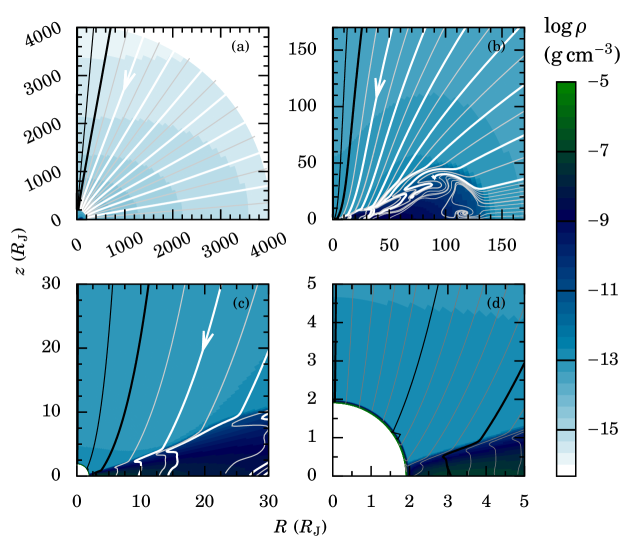
Figure 1: Density structure (colour) and flow pattern (lines) from ${R_{\textrm{Hill}}}$ to $R_{\textrm{p}}$ scales. The streamlines start at ${R_{\textrm{Hill}}}$ at $\theta_{\textrm{init}}\equiv\theta({r_{\textrm{max}}})=0.5$° and from 5° up to 85° in steps of 5° (panels (a)–(d); thick: multiples of 10°) or also 1° (panels (b) and (d)). Due to angular momentum conservation, the arrow-bearing streamline with $\theta_{\textrm{init}}=20$°, for example, hits the CPD with $\theta\gg 20$° and not on the planet surface. Only gas within $\theta_{\textrm{init}}\approx 10$° shocks with sufficient velocity to generate H $\alpha$ ($\theta_{\textrm{init}}=0.5$, 5, 10°: black).

Figure 1 shows the large- and small-scale structure of the flow and the gas density. At the Hill sphere, the gas is in radial freefall at all latitudes, so that all the gas entering the Hill sphere will accrete onto (that is, become part of) the planet or CPD. For comparison, in 3D a fraction of the flow would flow back out on perturbed horseshoe orbits (Machida et al., 2008; Lambrechts & Lega, 2017; Maeda et al., 2022). Therefore, our inflow rate corresponds to the net inflow in 3D (see also Section 3.3).

Everywhere outside of the planet and CPD (i.e., where the gas is infalling), the radiative flux is almost purely radial (see Appendix D). Accordingly, the temperature is approximately constant along $\theta$ at a given radius. Then, the density stratification leads to a positive pressure gradient: $dP/d\theta\propto d\rho/d\theta\propto-d\rho/dz>0$. In turn, the pressure gradient pushes the gas outside of $r\approx 100~{}R_{\textrm{J}}$ poleward. It does so by at most 5° compared to a radial trajectory, and inside of $r\approx 100~{}R_{\textrm{J}}$, angular momentum conservation deflects the gas outwards. This deviation from a radial trajectory becomes more important closer in to the planet. For example, the streamline that started at $\theta_{\textrm{init}}\equiv\theta({r_{\textrm{max}}})=20$° at ${R_{\textrm{Hill}}}$ joins the CPD at $\theta=73{\mbox{\textdegree}}\gg\theta_{\textrm{init}}$ (Figure 1c). The gravitational potential energy of the gas serves to increase all three components of the velocity.

The key result seen in Figure 1 is that most streamlines reach the CPD at a large distance (hundreds of Jupiter radii) from the planet. Only a small fraction of the total mass influx from ${R_{\textrm{Hill}}}$ falls in close to the planet. This consequence of angular momentum conservation was seen by Tanigawa et al. (2012) with a very different set-up (Table 1). Independent work by Chen & Bai (in prep.) also finds this. It has been derived analytically for ballistic (pressure-free) trajectories starting from an outer edge in solid-body rotation, in the context of star formation (Ulrich, 1976; Mendoza et al., 2009). We have now obtained that most gas reaches the CPD far from the planet also when radiation transfer and thermal effects are included. This conclusion will be seen to hold for other parameter combinations.

Two partial mass influx rates are of interest, in particular for simulations that cannot resolve down to these scales. One is the gas falling directly onto the planetary surface:

$$\dot{M}_{\textrm{p,\,direct}}=4\pi R_{\textrm{p}}^{2}\int\rho(\theta)v_{r}(\theta)\sin\theta\,d\theta,$$ (9)

integrated at $r=R_{\textrm{p}}$ from the pole ($\theta=0$) down to the surface of the CPD where it connects to the planetary surface (in a so-called “boundary layer”; e.g., Kley, 1989; Hertfelder & Kley, 2017). This gives $\dot{M}_{\textrm{p,\,direct}}=3.0\times 10^{-8}~{}M_{\textrm{J}}\,\textrm{yr}^{-1}$ at $R_{\textrm{p}}=2~{}R_{\textrm{J}}$, where the CPD is roughly 10° thick. Since $\dot{M}_{\textrm{Hill,\,net}}=6.9\times 10^{-6}~{}M_{\textrm{J}}\,\textrm{yr}^{-1}$ (Table 2), only $\dot{M}_{\textrm{p,\,direct}}/\dot{M}_{\textrm{Hill,\,net}}=0.4$ percent of the gas entering the Hill sphere reaches the planetary surface directly. The expressions of Adams & Batygin (2022) predict a qualitatively similar result, with differences because they assumed at the Hill sphere a uniform density and solid-body rotation, and neglected pressure forces (cf. our Section 4.1), as in Mendoza et al. (2009).

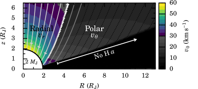
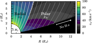
Figure 2: Components of the velocity (in $\textrm{km}\,\textrm{s}^{-1}$) perpendicular to each shock $v_{0}$: radial $v_{r}$ around streamlines that will hit the planet surface, and polar $v_{\theta}$ for the ones that will hit the CPD. H $\alpha$ emission requires $v_{0}>{v_{\textrm{H}\,\alpha,\,\textrm{crit}}}\approx 30~{}\textrm{km}\,\textrm{s}^{-1}$ (solid grey streamlines; black dotted otherwise). Streamlines start at ${R_{\textrm{Hill}}}$ in steps of $\Delta\theta=1{\mbox{\textdegree}}$. Left: Fiducial simulation ($M_{\textrm{p}}=2~{}M_{\textrm{J}}$); right: HigherMass ($M_{\textrm{p}}=5~{}M_{\textrm{J}}$). The two velocity scales differ but both have colours only above ${v_{\textrm{H}\,\alpha,\,\textrm{crit}}}$. In both cases, the preshock velocity over the whole free planetary surface is high enough for H $\alpha$ emission, but only a part of the CPD emits.

The second partial mass flow rate, $\dot{M}_{\textrm{H}\,\alpha}$, measures the mass inflow able to generate H $\alpha$, that is, the gas whose preshock velocity $v_{0}$ exceeds ${v_{\textrm{H}\,\alpha,\,\textrm{crit}}}$. To determine $\dot{M}_{\textrm{H}\,\alpha}$, we look at the component of the velocity that is perpendicular to the planetary surface and to the CPD surface, shown in Figure 2. For the shock at the surface of the planet, the normal component is the radial velocity $v_{r}$ because the planet surface is nearly spherical. Even for this small mass of $M_{\textrm{p}}=2~{}M_{\textrm{J}}$, over the whole free surface of the planet, the gas is fast enough to generate H $\alpha$ (Equation (2)). Out to at least $\approx 10~{}R_{\textrm{J}}$ for the CPD in our simulation, the CPD (shock) surface is nearly radial and is flat, such that the normal component is nearly equal to the polar velocity $v_{\theta}$ evaluated above the shock surface. For simplicity, we take $v_{0}=v_{\theta}$. We identify the largest radius ${r_{\textrm{30~{}$\textrm{km}\,\textrm{s}^{-1}$}}}$ on the CPD out to which $v_{0}\geqslant{v_{\textrm{H}\,\alpha,\,\textrm{crit}}}$ and integrate the mass flux at that radius from the pole down to the surface of the CPD:

$$\dot{M}_{\textrm{H}\,\alpha}=4\pi{r_{\textrm{30~{}$\textrm{km}\,\textrm{s}^{-1}$}}}^{2}\int\rho(\theta)v_{r}(\theta)\sin\theta\,d\theta.$$ (10)

Due to time-independence, this is equivalent to an integral over the shock surfaces. We find a maximum radius ${r_{\textrm{30~{}$\textrm{km}\,\textrm{s}^{-1}$}}}=3.3~{}R_{\textrm{J}}$ and a CPD height of 14° there. This yields $\dot{M}_{\textrm{H}\,\alpha}=4.7\times 10^{-8}~{}M_{\textrm{J}}\,\textrm{yr}^{-1}$, or $\dot{M}_{\textrm{H}\,\alpha}/\dot{M}_{\textrm{Hill,\,net}}=0.7$ percent.

Both $\dot{M}_{\textrm{p,\,direct}}$ and $\dot{M}_{\textrm{H}\,\alpha}$ are small fractions of $\dot{M}_{\textrm{Hill,\,net}}$. Correspondingly, they originate from a narrow polar region, in which the specific angular momentum of the gas $j_{z}=Rv_{\phi}\propto r^{2}\sin^{2}\theta$ (Equation (3)) is low. Indeed, tracing the streamlines that define $\dot{M}_{\textrm{p,\,direct}}$ and $\dot{M}_{\textrm{H}\,\alpha}$ back to ${r_{\textrm{max}}}$, we find starting angles of $\theta_{\textrm{init}}\approx 7$° and $\theta_{\textrm{init}}\approx 9$°, as seen in Figure 2.

Comparing $\dot{M}_{\textrm{H}\,\alpha}$ and $\dot{M}_{\textrm{p,\,direct}}$, we see that $(1-\dot{M}_{\textrm{p,\,direct}}/\dot{M}_{\textrm{H}\,\alpha})\approx 60$ percent of the total H $\alpha$-generating gas falls on the CPD surface and not on the planet. This assumes that all of $\dot{M}_{\textrm{p,\,direct}}$ produces H $\alpha$, which holds. However, the local H $\alpha$ flux $F_{\textrm{H}\,\alpha}$ depends strongly on $v_{0}$ (crudely, $F_{\textrm{H}\,\alpha}\sim{v_{0}}^{3}$; Aoyama et al., 2018), so that it is not clear a priori whether the CPD or the planetary surface dominates the total emission. We look at this in more detail in the next section.

4.2 Approximate H $\alpha$ emission

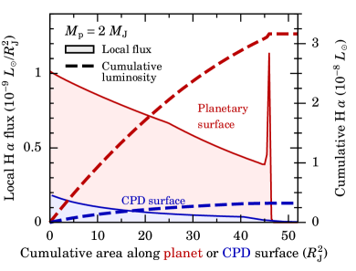
Figure 3: Flux from the accretion shocks on the planet surface (solid red curve with a filled area) and on the CPD surface (blue) as a function of the cumulative area along the planetary surface, starting at the pole, or along the CPD surface, starting at the planet at $R_{\textrm{p}}=2~{}R_{\textrm{J}}$ (Equation (11)). With this $x$ axis, the area under each curve is proportional to its contribution to the luminosity. The spike comes from the high-velocity surface flow but barely contributes to the total flux, contrary to what Takasao et al. (2021) find (see Section 5.2). Dashed curves show the cumulative integral of each contribution (right axis).

We estimate the observable H $\alpha$ luminosity from the planet-surface and CPD-surface shocks. Detailed 2D radiation transport of the generated H $\alpha$ is beyond the scope of this paper. However, based on Marleau et al. (2022) and for $f_{\textrm{d/g}}=10^{-4}$, we expect the incoming gas and dust to be very optically thin to H $\alpha$ photons for a mass influx rate $\dot{M}_{\textrm{Hill,\,net}}\sim 10^{-5}~{}M_{\textrm{J}}\,\textrm{yr}^{-1}$ or even much higher. Also, given that ${q_{\textrm{th}}}\gtrsim 1$ planets open gaps, extinction by the PPD is possibly negligible. Therefore, summing the local H $\alpha$ production along the planetary and CPD surfaces (the radiative source terms) gives a reasonable estimate of the luminosity leaving the system.

We display in Figure 3 the H $\alpha$ flux per emitting area $F_{\textrm{H}\,\alpha}$, which depends only on the local preshock density $\rho_{0}$ and preshock velocity $v_{0}$ above either shock. We use the data of Aoyama et al. (2018) for $F_{\textrm{H}\,\alpha}(\rho_{0},v_{0})$. For the surface shock, the flux is plotted against the distance from the pole, and for the CPD shock, outwards from the surface of the planet, where the CPD begins. Instead of the linear distance, we use the respective cumulative areas (including both hemispheres):

$$A_{\textrm{plnt~{}surf}}(\theta) =\int_{0}^{\theta}4\pi R_{\textrm{p}}^{2}\sin\theta^{\prime}\,d\theta^{\prime},$$ (11a)

$$A_{\textrm{CPD~{}surf}}(r) =\int_{R_{\textrm{p}}}^{r}4\pi r^{\prime}\sin\theta\,dr^{\prime},$$ (11b)

where we have assumed a $\theta=\mbox{constant}$ CPD surface in Equation (11b), which holds approximately for the region whose H $\alpha$ emission dominates (see Figure 2). For the actual analysis, we look for the temperature peak (the Zel’dovich spike) for each $r=\mbox{constant}$ ring in the $r$–$\theta$ plane, and use the cell above it to define the surface. With Equation (11) to measure distance, the ratio of the areas under the curves gives the relative contribution of each shock. Emission comes from the exposed planetary surface from the pole down to the surface of the CPD at ${\theta_{\textrm{max}}}$, which corresponds to a filling factor $f_{\textrm{fill}}=1-\cos{\theta_{\textrm{max}}}=0.83$, and from the CPD from the planetary radius out to $r\approx{r_{\textrm{30~{}$\textrm{km}\,\textrm{s}^{-1}$}}}\approx 3.3~{}R_{\textrm{J}}$ (as found in Section 4.1). The region without emission is labelled in Figure 2.

The integrated luminosities (dashed lines in Figure 3) are $L_{\textrm{H}\,\alpha}=3.2\times 10^{-8}~{}{L_{\odot}}$ for the planetary surface shock and $L_{\textrm{H}\,\alpha}=0.45\times 10^{-8}~{}{L_{\odot}}$ for the contribution by the CPD. Approximately, ignoring the angular dependence of the radiation by summing the two terms, an observer looking at the system would see an H $\alpha$ luminosity $L_{\textrm{H}\,\alpha}\approx 3.7\times 10^{-8}~{}{L_{\odot}}$. We compare this to the observations of PDS 70 b in Section 5.1. The supersonic surface flow on the CPD, discussed in Appendix B, causes a local spike in the emission (filled region in Figure 3). However, this thin layer contributes negligibly to the integrated emission. This contrasts strongly with the results of Takasao et al. (2021), to which we return in Section 5.2.

Figure 3 shows that the planetary surface shock largely dominates the H $\alpha$ emission. The preshock densities, $\rho_{0}\sim 10^{-13}~{}\textrm{g}\,\textrm{cm}^{-3}$, which depend only weakly on position, are similar to within 0.1 dex between both shocks, and the emitting areas are similar (near $45~{}R_{\textrm{J}}^{2}$). However, the difference in the preshock velocities is much more consequential. The velocities are different in part because the emitting region of the CPD is at slightly greater $r$ (Figure 2: $r\approx 3~{}R_{\textrm{J}}$ and $r\approx(3$–10) $R_{\textrm{J}}$ for the two simulations) than the planet surface ($R_{\textrm{p}}=2~{}R_{\textrm{J}}$). The other, and more important, factor is that for the CPD, the shock velocity (i.e., the component orthogonal to the shock surface) is the polar velocity $v_{\theta}$, and this is even smaller than the local radial velocity $v_{r}$.

We can compare the H $\alpha$ luminosity from the free planetary surface to the luminosity expected from purely radial accretion at ${v_{\textrm{ff}}}$ for the same $\dot{M}_{\textrm{p,\,direct}}$ and $f_{\textrm{fill}}$. Explicitly, the combination $(\dot{M}_{\textrm{p,\,direct}},M_{\textrm{p}},R_{\textrm{p}},f_{\textrm{fill}})$ that we have here implies an average preshock number density $n_{0}=X\dot{M}_{\textrm{p,\,direct}}/(4\pi R_{\textrm{p}}^{2}f_{\textrm{fill}}{v_{\textrm{ff}}}m_{\textrm{H}})=6.3\times 10^{10}~{}\textrm{cm}^{-3}$ (Equation (A9) of Aoyama et al. 2020) and thus $L_{\textrm{H}\,\alpha}^{\prime}=4\pi R_{\textrm{p}}^{2}f_{\textrm{fill}}\times F_{\textrm{H}\,\alpha}(n_{0},{v_{\textrm{ff}}})=4.7\times 10^{-8}~{}{L_{\odot}}$, which is higher by 50 % than what we found. The difference is due mainly to the strong dependence of $F_{\textrm{H}\,\alpha}$ on $v_{0}$ with, roughly, $F_{\textrm{H}\,\alpha}\propto v_{0}^{3}$ (Aoyama et al., 2018). Indeed, in our simulation, the radial velocity at the pole is equal to the freefall value ${v_{\textrm{ff}}}=59.5$ $\textrm{km}\,\textrm{s}^{-1}$, but at the equator it is lower by about 30 %. This is because the gas gains more velocity in $\theta$ and in $\phi$ further away from the pole, with the three components summing up to $v_{r}^{2}+v_{\theta}^{2}+v_{\phi}^{2}={v_{\textrm{ff}}}^{2}$ everywhere in the free-falling region by conservation of energy. In other words, centrifugal forces due to angular-momentum conservation are slowing down the infalling gas at low latitudes. This reduction of the preshock velocity leads to less emission ($\sim\rho_{0}v_{0}^{3}$) for the same total mass flow rate ($\sim\rho_{0}v_{0}$) compared to the simple assumption of radial freefall.

4.3 Varying the incoming angular momentum

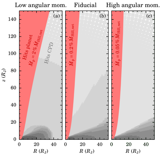
Figure 4: Fraction of the total inflow rate reaching the planet surface for different amounts of angular momentum at the Hill sphere, probed by varying the position of the outer radius of the simulation domain: ${r_{\textrm{max}}}/{R_{\textrm{Hill}}}=0.7$, 1.0 (fiducial run), 1.3 (left, middle, and right panel, respectively). In all cases, the gas flows inwards for all angles from ${r_{\textrm{max}}}$ down to the planet or CPD. The greyscale shows the density (logarithmic). Each simulation extends to ${r_{\textrm{max}}}=4100~{}R_{\textrm{J}}$.

The specific angular momentum of the gas entering the domain depends on the choice of the outer radius ${r_{\textrm{max}}}$ (Equation (3)). As argued in Section 3.1, setting ${r_{\textrm{max}}}={R_{\textrm{Hill}}}$ is a natural choice for simulations assuming axisymmetry around the planet, but it remains approximate. The incoming angular momentum sets what fraction of the gas can reach the planet, and in general it might determine whether an outflow near the midplane occurs or not. Here, we have infall at all angles, but an outflow does occur in the azimuthal average of 3D simulations (e.g. Schulik et al., 2020).

Therefore, we performed two additional simulations with the same parameters except for ${r_{\textrm{max}}}=0.7{R_{\textrm{Hill}}}$ and ${r_{\textrm{max}}}=1.3{R_{\textrm{Hill}}}$, named LowAngMom and HighAngMom, to give the accreting gas less or more angular momentum, respectively. We have chosen planet radiinear $R_{\textrm{p}}=2~{}R_{\textrm{J}}$ by keeping ${r_{\textrm{min}}}=1.9~{}R_{\textrm{J}}$, with the exact values set by how much mass is accreted and how it cools until a quasi-steady-state is established as described in Section 3.2.4. The radii turn out to be respectively $R_{\textrm{p}}=2.15$ and 1.95 $R_{\textrm{J}}$, which is similar enough for our purposes, especially since the radius does not affect directly the infall of matter (see also Section 5.3). Since ${R_{\textrm{Hill}}}=1.33{H_{P}}$ (Table 2), LowAngMom has ${r_{\textrm{max}}}\approx{H_{P}}$. We took ${N_{\theta}}=51$ instead of ${N_{\theta}}=181$ since it does not influence the accretion flow. We find that also for these simulations the radial velocity of the gas at ${r_{\textrm{max}}}$ quickly reaches and remains at the free-fall velocity for all angles. Because we keep the density at ${r_{\textrm{max}}}$ the same, the mass influxes at the Hill sphere are somewhat lower and higher respectively, with $\dot{M}_{\textrm{Hill,\,net}}=5\times 10^{-6}~{}M_{\textrm{J}}\,\textrm{yr}^{-1}$ for LowAngMom and $\dot{M}_{\textrm{Hill,\,net}}=9\times 10^{-6}~{}M_{\textrm{J}}\,\textrm{yr}^{-1}$ for HighAngMom, instead of $\dot{M}_{\textrm{Hill,\,net}}=7\times 10^{-6}~{}M_{\textrm{J}}\,\textrm{yr}^{-1}$ for the fiducial run. As summarised in Section 3.3, judging from Marleau et al. (2017) this difference in density will not influence the flow pattern.

Figure 4 compares the flow of the gas on scales of $r\sim 50$–$150~{}R_{\textrm{J}}\sim 0.01$–$0.03{R_{\textrm{Hill}}}$ for ${r_{\textrm{max}}}/{R_{\textrm{Hill}}}=0.7$, 1.0, 1.3. As expected, with larger ${r_{\textrm{max}}}$, only gas from a smaller cone around the pole reaches the planetary surface directly (highlighted in pink). The starting angle of the last streamline hitting the planet surface is $\theta_{\textrm{init}}=15.8$° for LowAngMom and $\theta_{\textrm{init}}=3.9$° for HighAngMom, which bracket the corresponding $\theta_{\textrm{init}}=7.1$° for the fiducial case. The same applies to the mass fluxes relative to the respective $\dot{M}_{\textrm{Hill,\,net}}$, which are $\dot{M}_{\textrm{p,\,direct}}/\dot{M}_{\textrm{Hill,\,net}}=2.4$ percent for LowAngMom and $\dot{M}_{\textrm{p,\,direct}}/\dot{M}_{\textrm{Hill,\,net}}=0.052$ percent for HighAngMom; the fiducial case had $\dot{M}_{\textrm{p,\,direct}}/\dot{M}_{\textrm{Hill,\,net}}=0.7$ percent.

Thus, at fixed $\dot{M}_{\textrm{Hill,\,net}}$, $\dot{M}_{\textrm{p,\,direct}}$ depends sensitively on ${r_{\textrm{max}}}$ but, overall, the fraction of $\dot{M}_{\textrm{Hill,\,net}}$ that shocks on the planetary surface is at most of order of one percent. The dependence of $\dot{M}_{\textrm{H}\,\alpha}$ on ${r_{\textrm{max}}}/{R_{\textrm{Hill}}}$ will be similar. We discuss this further in Section 5.3. For reference, we obtain $L_{\textrm{H}\,\alpha}=1.0\times 10^{-7}$ and $7.3\times 10^{-9}~{}{L_{\odot}}$ for LowAngMom and HighAngMom, respectively, again bracketing the fiducial case with its $L_{\textrm{H}\,\alpha}=3.7\times 10^{-8}~{}{L_{\odot}}$.

4.4 Varying the planet mass

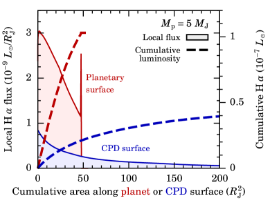
Figure 5: As in Figure 3 but for 5 $M_{\textrm{J}}$. The total is $L_{\textrm{H}\,\alpha}=1.4\times 10^{-7}~{}{L_{\odot}}$. The planetary surface is twice as bright as the CPD.

Short of doing a full exploration of the whole parameter space, we consider also a higher $M_{\textrm{p}}$. The planetary mass is an important parameter that controls the dynamics of the gas. We wish to see whether here too only a fraction of the gas entering the Hill sphere falls directly onto the planet, and whether the planetary surface still dominates the H $\alpha$ emission relative to the CPD as it does for $M_{\textrm{p}}=2~{}M_{\textrm{J}}$ (Figure 3). A priori, especially the latter could change for higher masses because $v_{0}$ scales to zeroth order with ${v_{\textrm{ff}}}\propto r^{-1/2}$, which will lead to a larger H $\alpha$-emitting area on the CPD.

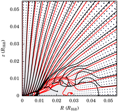
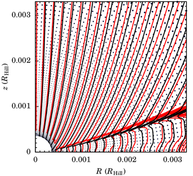
Figure 6: Comparison of the flow in the $M_{\textrm{p}}=5$-$M_{\textrm{J}}$ simulation (black) to the fiducial 2-$M_{\textrm{J}}$ run (red). Streamlines are for $\theta_{\textrm{init}}=0$, 5, …, 90° (left) or $\theta_{\textrm{init}}=0$, 1, 2°, …(right). The axes, different for each panel, are scaled by the respective Hill radius of each simulation. Dark blue dots show the cell centers in the 5-$M_{\textrm{J}}$ run.

We therefore simulate an accreting planet as in the fiducial run but with $M_{\textrm{p}}=5~{}M_{\textrm{J}}$ and name this HigherMass. Bae et al. (2019) used this value for PDS 70 b. We set again ${r_{\textrm{max}}}$ equal to ${R_{\textrm{Hill}}}(M_{\textrm{p}})$, and use ${N_{\theta}}=51$. The other parameters are the same, leading to a large ${q_{\textrm{th}}}=18$. Figure 6 shows that the flow pattern for the 5-$M_{\textrm{J}}$ simulation is similar to the one of the 2-$M_{\textrm{J}}$ simulation. Even at this lower resolution in $\theta$, a thin ($\sim 1$°) fast inward surface flow is seen again. Repeating the analysis above, we find that for $5~{}M_{\textrm{J}}$ only $\dot{M}_{\textrm{p,\,direct}}/\dot{M}_{\textrm{Hill,\,net}}=1.2$ percent of $\dot{M}_{\textrm{Hill,\,net}}=1.4\times 10^{-5}~{}M_{\textrm{J}}\,\textrm{yr}^{-1}$ reaches the planet directly, and that $\dot{M}_{\textrm{H}\,\alpha}/\dot{M}_{\textrm{Hill,\,net}}=7$ percent shocks with $v\gtrsim{v_{\textrm{H}\,\alpha,\,\textrm{crit}}}$. For $M_{\textrm{p}}=2~{}M_{\textrm{J}}$, we recall that we had smaller fractions of 0.4 and 0.7 percent, respectively.

In Figure 5, we show the H $\alpha$ emission from the planetary surface and the CPD, as in Figure 3. Again, the inward flow below the CPD surface does not generate an overall important H $\alpha$ flux; there is a local spike but its relative contribution is negligible. The planetary surface generates $L_{\textrm{H}\,\alpha}=1.2\times 10^{-7}~{}{L_{\odot}}$ and the CPD surface generates $L_{\textrm{H}\,\alpha}=0.54\times 10^{-7}~{}{L_{\odot}}$. Summing the two terms again in lieu of detailed radiation transport yields in total $L_{\textrm{H}\,\alpha}\approx 1.7\times 10^{-7}~{}{L_{\odot}}$. Thus, the CPD surface emits about 30 percent of the total flux, up from 15 percent in the 2-$M_{\textrm{J}}$ case. This relative increase is because $v_{0}>{v_{\textrm{H}\,\alpha,\,\textrm{crit}}}$ out to a cylindrical radius of $R\approx 9~{}R_{\textrm{J}}$ instead of $R\approx 3~{}R_{\textrm{J}}$ in the fiducial case (see the coloured regions in both panels of Figure 2).

5 Discussion

Our main results are that (a) only a small fraction of the net mass flux into the Hill sphere falls directly onto the planet, (b) only a slightly larger fraction produces any H $\alpha$ (Figures 1 and 2), and (c) the emitted H $\alpha$ comes from both the planetary and the CPD surfaces, and not from the fast flow beneath the CPD surface (Figure 2). Our simulations were conducted in 2.5D but Tanigawa et al. (2012) obtained qualitatively the same Hill-sphere flow structure in their larger-scale isothermal 3D simulations. This lends support to our 2.5D approach and suggests that these findings are robust. The advantage of 2.5D is that it makes it computationally much more accessible not to smooth the gravitational potential while including radiation transport. This allowed us to simulate down to sub-planet scales, crucial for calculating $L_{\textrm{H}\,\alpha}$ since the highest-velocity regions strongly dominate the emission.

In Section 5.1, we look at PDS 70 b. In Section 5.2, we compare our results with other predictions of H $\alpha$ emission from planets accreting other than by magnetospheric accretion (for the latter, see discussion in Aoyama et al. 2021). Finally, in Section 5.3 we comment on a few aspects of our models.

5.1 Comparison with PDS 70 b

As a check, we compare the $L_{\textrm{H}\,\alpha}$ estimated from the simulations with the observational data for PDS 70 b. This planet had motivated our parameter choices (Table 2). Assuming that the H $\alpha$ photons are leaving the system isotropically, its measured luminosity is $L_{\textrm{H}\,\alpha}=7\times 10^{-7}~{}{L_{\odot}}$ (Zhou et al., 2021; Sanghi et al., 2022). At such luminosities, absorption within the system is likely unimportant for a very wide range of dust opacities (Marleau et al., 2022), and absorption by the PPD is more likely to be low given that the planet is found in a gap. Therefore, a direct comparison is meaningful.

For the different runs, we obtained $L_{\textrm{H}\,\alpha}\sim 10^{-8}$–$10^{-7}~{}{L_{\odot}}$, which is 10–100 times smaller than the observationally derived value. This is in fact satisfactory given that we took nominal model parameters (Table 2) from the literature without efforts to match the $L_{\textrm{H}\,\alpha}$. Reducing the incoming angular momentum or radius of the planet, or using $M_{\textrm{p}}=12$ $M_{\textrm{J}}$ as in Dong et al. (2021), would make it easy to raise our $L_{\textrm{H}\,\alpha}$ closer to the measured value. Beyond this, magnetospheric accretion columns, if present, could also be contributing to the flux.

5.2 Comparison to other predictions of H $\alpha$

Only few studies so far predict the H $\alpha$ emission of forming planets. Thanathibodee et al. (2019) applied magnetospheric-accretion radiation-transfer models for stars to the planetary regime, but Szulágyi & Ercolano (2020) were the first to present hydrogen-line luminosities based on 3D radiation-hydrodynamics simulations. However, their smoothing of the gravitational potential (Table 1) makes their results challenging to interpret, as Aoyama et al. (2020, 2021) discuss. Therefore, we restrict our comparison here to the work of Takasao et al. (2021), who also set ${\varepsilon_{\textrm{grav}}}=0$.

We follow a similar approach to Takasao et al. (2021) to calculate the H $\alpha$ emission from the simulation data, by integrating the local H $\alpha$ flux predicted by Aoyama et al. (2018) as a function of the preshock velocity and density (Section 4.2). However, Takasao et al. (2021) find that nearly 95 percent of the H $\alpha$ emitted from the planetary surface comes from an approximately 10–$15$°-thick surface layer of the CPD where the flow hits the planetary surface (see their schematic Figure 13). This differs significantly from our results, in which the sub-CPD-surface flow is very thin ($\sim 1$°) and contributes negligibly to the total luminosity (Figures 3 and 5).

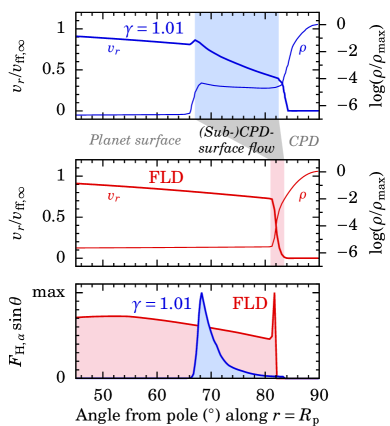
Figure 7: Structures in the $\gamma=1.01$ hydrodynamics simulation of Takasao et al. (2021) compared to ours (with FLD). Top and middle panels: Radial velocity immediately above the planet surface, normalised to the respective ${v_{\textrm{ff}}}$ (Equation (2)), and density (normalised to the maximum, i.e., midplane density) in their (top panel; blue curves) and our (middle panel; pink curves) simulations. Bottom panel: Local H $\alpha$ flux times $\sin\theta$, normalised to the respective maxima. This way, the relative areas under the curves are proportional to their contribution to the total flux.

To understand the difference, we compare in Figure 7 the radial velocity and the density at $r=R_{\textrm{p}}$ in the work of Takasao et al. (2021) (top panel) and our work (middle panel). Three similar zones are present in both work: the free surface of the planet from the pole down to (geometrically, or “up to” in angle) $\theta=67.5{\mbox{\textdegree}}$ in their case or $\theta=80{\mbox{\textdegree}}$ in ours; the fast (sub-)CPD-surface flow, which is quite thick in their case and thin in ours (coloured regions in Figure 7ab); and the CPD connecting to the planet surface, at $\theta\gtrsim 83{\mbox{\textdegree}}$ for both. In both simulations the radial velocity above the planet is equal to ${v_{\textrm{ff},\,\infty}}$ at the pole (not shown) and decreases with $\theta$, as discussed in Section 4.2. Also, in both cases the density increases quickly in the CPD zone, as expected for (approximately) isothermal structures (see Figure 10) in hydrostatic equilibrium.

However, there is a large difference in the layer located between the free-falling gas and the CPD. Takasao et al. (2021) obtained a zone roughly 10–$15{\mbox{\textdegree}}$ thick in which the radial velocity decreases only slowly by half, which they called a “postshock, converged accretion flow”. However, we find a zone that is only a few degrees thin and in which the radial velocity decreases quickly as a function of distance below the surface. In our simulations too is there a visible convergence of the postshock accretion flow, seen as the approximately constant-$\theta$ segments of the sub-CPD-surface streamlines in Figure 6. However, this converged flow has a smaller $|v_{r}|$, is thin, and involves relatively little mass. Since the flow is the same while more than doubling the mass ($M_{\textrm{p}}=2$ vs. 5 $M_{\textrm{J}}$), it most likely does not matter that Takasao et al. (2021) set an even higher mass $M_{\textrm{p}}=12~{}M_{\textrm{J}}$.

This qualitative difference in the flows at the CPD surface must come instead from the different thermodynamics that Takasao et al. (2021) assumed, namely no radiative transfer but an adiabatic equation of state with $\gamma$ close to, but above, unity. Even though $\gamma$ is close to the isothermal value of unity, their adiabatic equation of state leads to a thick and hot post-shock region surrounding the CPD, as their Figure 6 shows. Consequently, the radial velocity remains high after the shock in $\theta$, so that the gas hits the planet surface quickly: the gas is subsonic but the Mach number is large, so that the absolute velocity is high. On the contrary, with radiative transfer, the gas cools quickly and the density increases much more across the shock. By mass conservation, the postshock radial velocity is correspondingly smaller, which decreases significantly the amount of emission.

Figure 7c shows the local H $\alpha$ line emission at $r=R_{\textrm{p}}=2~{}R_{\textrm{J}}$ as a function of angle from the pole. We plot $F_{\textrm{H}\,\alpha}\times\sin(\theta)$, as in Equation (13) of Takasao et al. (2021), and normalise the curves from Takasao et al. (2021) and our simulation independently to their respective maximum. This way, the areas under the curves are proportional to the contribution of each region to the total flux from a model. This shows very clearly that in the simulation of Takasao et al. (2021), only the sub-CPD-surface flow, where it hits the planets, generates appreciable amounts of H $\alpha$, whereas in our case that zone is negligible for the integral (seen also in Figures 3 and 5).

In our finding that only a small fraction of the large-scale flow falls directly onto the planet, however, we agree qualitatively with Takasao et al. (2021). Excluding the radial flow below the CPD surface, the accretion rate directly onto the planetary surface in their case is $\dot{M}_{\textrm{p,\,direct}}\approx 3\times 10^{-10}~{}M_{\textrm{J}}\,\textrm{yr}^{-1}$, which is 0.2 percent of their net mass influx rate $\dot{M}_{\textrm{Hill,\,net}}=2\times 10^{-7}~{}M_{\textrm{J}}\,\textrm{yr}^{-1}$. This is smaller than but similar to our fractions for 2 and 5 $M_{\textrm{J}}$ (0.4 and 1.2 percent), with the difference likely coming from their choice of a purely vertical mass flow at their ${r_{\textrm{max}}}=100~{}R_{\textrm{p}}$.

We conclude that including radiation transfer in hydrodynamical simulations is important for accurate predictions of H $\alpha$ emission because of their sensitivity to the velocity structure. The flow in the large-scale, supersonic region can likely be well captured by isothermal simulations, but the post-shock behaviour of the gas depends on the thermodynamics. Smoothing-free 3D simulations in the high-mass (high-${q_{\textrm{th}}}$), low-$R_{\textrm{p}}/{R_{\textrm{Hill}}}$ regime would be a worthwhile complement to the existing work (Table 1).

5.3 Further aspects within and beyond our model

We comment on a few aspects within or beyond our model: Regions traced by the H $\alpha$.—The results of Section 4.4 suggest that as the planet mass increases, the contribution of the CPD to the total H $\alpha$ becomes increasingly important. However, the two terms remain of the same order of magnitude, and if the CPD is thicker than in Figure 6, the reduced shock velocity would lead to a smaller contribution. Modelling of the line shapes should therefore take both components into account.

Varying the planetary radius.—We can do this approximately without additional simulations by measuring the $\dot{M}$’s according to Equations (9) or (10) at a different $r=R_{\textrm{p}}^{\prime}$, and similarly beginning at $R_{\textrm{p}}^{\prime}$ the outwards integration of the H $\alpha$ emission along the CPD surface. To first order, the choice of $R_{\textrm{p}}$ will not affect the supersonic flow. In a similar approach, Takasao et al. (2021) set an open boundary at their ${r_{\textrm{min}}}$ and used the density and velocity there to calculate the H $\alpha$ emission that would come from a shock at that position. Doing this, we find roughly $L_{\textrm{H}\,\alpha}\propto 1/R_{\textrm{p}}$, which can be used to scale approximately the results of one simulation to other $R_{\textrm{p}}$ values.

Choice of ${r_{\textrm{max}}}$.—We have varied ${r_{\textrm{max}}}$ by 30 percent, with the case ${r_{\textrm{max}}}=1.3{R_{\textrm{Hill}}}$ corresponding to ${r_{\textrm{max}}}\approx{H_{P}}$. It would be surprising if 3D simulations corresponded effectively to a much larger ${r_{\textrm{max}}}$, but the effective ${r_{\textrm{max}}}$ could conceivably be smaller. Then, a larger fraction of $\dot{M}_{\textrm{Hill,\,net}}$ would reach the planet directly and emit H $\alpha$.

Models of 1D planet structure.—Global formation models use $\dot{M}_{\textrm{Hill,\,net}}$ to set the ram pressure at the surface of the planet when calculating its radius and luminosity (Mordasini et al., 2012b). However, this is an incorrect assumption, since only the much smaller rate $\dot{M}_{\textrm{p,\,direct}}\ll\dot{M}_{\textrm{Hill,\,net}}$ will set the pressure on the surface of the planet, which could affect its postformation luminosity (e.g., Mordasini, 2013; Berardo et al., 2017). In our simulations so far the (radial) ram pressure $P_{\textrm{ram}}(\theta)=\rho(\theta)v_{r}(\theta)^{2}$ turns out to be almost constant with polar angle (not shown), so that the reduced ram pressure could be easily included in 1D planet models. However, an appropriate treatment of the boundary layer with its ${f_{\omega}}$-dependent transfer of mass, angular momentum, and energy would be needed (e.g., Dong et al., 2021).

Other hydrogen lines.—Other hydrogen lines such as H $\beta$, Pa $\beta$, or Br $\gamma$ have been observed at a few planetary-mass objects such as Delorme 1 (AB)b (Eriksson et al., 2020; Betti et al., 2022a, b). These lines also require a similar minimum shock velocity ${v_{\textrm{crit}}}\approx{v_{\textrm{H}\,\alpha,\,\textrm{crit}}}=30~{}\textrm{km}\,\textrm{s}^{-1}$ to be emitted since their excitation energies are similar (Aoyama et al., 2018). Therefore, our analysis could have applied to the other lines as well.

Magnetospheric accretion.—If it proceeds as for young stars (e.g., Romanova et al., 2002; Hartmann et al., 2016), magnetospheric accretion is an interesting mechanism that could let the gas slide ballistically along the magnetic field lines connecting the inner edge of the CPD and the planet surface (Lovelace et al., 2011). This would lead to a shock at the planet surface at almost free-fall velocity and thus to H $\alpha$ emission. This would be in addition to what the direct infall $\dot{M}_{\textrm{p,\,direct}}$ generates, contrasting with the stellar case in which $\dot{M}_{\textrm{p,\,direct}}$ is essentially zero. In fact, magnetospheric accretion would let almost the same amount of H $\alpha$ be generated as in the 1D, spherically symmetric classical picture (e.g., Bodenheimer et al., 2000) since ultimately most accreting gas would reach the planet at (nearly) free-fall velocity.

Whether magnetospheric accretion from the CPD onto the planet actually takes place or not is not yet clear. It requires a few conditions to be met: (i) the CPD must be an accretion and not a decretion disc; (ii) the magnetic field of a young planet needs to be able to disrupt the CPD; and (iii) the gas must be sufficiently ionised to couple to the magnetic field (e.g., Keith & Wardle, 2014; Hasegawa et al., 2021). In the picture painted by Batygin (2018), in which gas falls towards the pole and a decretion disc, CPD disruption would not be needed and the apex of the magnetic field lines would increase the effective area of the planetary surface intercepting the flow. So far, interesting but only tentative scaling arguments support the main hypothesis of a sufficiently strong magnetic field (Christensen et al., 2009; Katarzyński et al., 2016), requiring further studies for a robust assessment. Further motivation might come tentative observational evidence for magnetospheric accretion in the somewhat older, essentially isolated object Delorme 1 (AB)b (Ringqvist et al., 2023).

6 Summary and conclusions

We studied the gas flow from the Hill radius down to the surface of a forming super-Jupiter planet able to generate hydrogen lines such as H $\alpha$. We performed axisymmetric, 2.5D radiation-hydrodynamical simulations in a vertical frame centered on the planet and following it on its orbit around the star. These simulations connect to global-disc simulations through the net mass inflow into the domain $\dot{M}_{\textrm{Hill,\,net}}$ and the angular momentum of the gas, both of which are input parameters here. We argued that the flow structure should depend only little on $\dot{M}_{\textrm{Hill,\,net}}$. Therefore, this should also apply to the partial accretion rates or the relative contributions to line emission by the planetary surface and the CPD surface.

Two important features compared to previous work are that we (i) included radiation transfer, with tabulated dust and gas opacities, to model correctly thermal effects that can influence the flow especially below the CPD-surface shock, and (ii) did not smooth the gravitational potential, and used a high spatial resolution close to the planetary surface ($\sim 0.01~{}R_{\textrm{J}}$). Whereas previous work with a non-zero smoothing length (e.g., Tanigawa et al., 2012) was concerned with the accretion of mass and angular momentum onto the CPD, we focus on the planet surface and the innermost regions of the CPD close to it.

We confirmed that most of the mass flux flowing towards the CPD and the planet forms an accretion shock on the surface of the CPD (Figure 2). Only a very small fraction of the order of a percent reaches the planet surface directly, and the fraction shocking at sufficiently high velocity ($v_{0}>{v_{\textrm{H}\,\alpha,\,\textrm{crit}}}=30~{}\textrm{km}\,\textrm{s}^{-1}$) to generate hydrogen lines such as H $\alpha$ is similarly small (Figure 4). We found that these results are robust to variations in the planetary mass and the angular momentum of the incoming gas. The large-scale flow pattern agrees qualitatively with 3D isothermal simulations with a smoothed gravitational potential (Tanigawa et al., 2012; Fung et al., 2019), lending support to our approach.

For all simulations, we estimated the H $\alpha$ emission through the non-equilibrium shock models of Aoyama et al. (2018). Our inclusion of radiative transfer keeps thin the fast flow beneath the CPD shock surface, so that only the free surfaces of the planet and the CPD emit shock tracers appreciably. This contrasts to the results of hydrodynamics-only simulations (Section 5.2), showing the importance of including radiation transfer while not smoothing the gravitational potential.

In summary, we have studied one aspect determining how many planets can be detected at accretion tracers such as H $\alpha$: what parts of the flow can generate accretion-line emission. However, we have not addressed the relation between this H $\alpha$-generating mass flux and the growth rate of the planet. This is a different question, beyond the scope of our work, and involves studying the timescale for mass transport in the CPD. In one limit, only what falls directly onto the planet will let it grow at a given time, but in the other the CPD would be able to feed the planet appreciably (Adams & Batygin, 2022). Dedicated simulations are required.

It is moreover a separate issue whether the statistics of known accreting planets matches expectations given our current understanding of planet formation and the empirical demographics of directly-imaged planets (e.g., Nielsen et al., 2019; Vigan et al., 2021). Both the migration and formation timescales influence this, but also the non-Gaussianity in the residuals in high-contrast images (Marois et al., 2008; see applefy by Bonse et al. 2023). A careful statistical treatment would be welcome (Dong et al., in prep.), as would more detections—for which there is hope thanks to instrumentational progress such as VIS-X (Haffert et al., 2021), KPIC (Delorme et al., 2021), or RISTRETTO (Chazelas et al., 2020), to name a few.

Appendix A Radial gridding

The radial gridding is made of three parts and is shown in Figure 8. The inner section at $r\in[{r_{\textrm{min}}},{r_{\textrm{min}}}+{L_{\textrm{u}}}]$ has 32 uniformly-spaced cells ${\Delta r_{\textrm{u}}}=0.001$ $R_{\textrm{J}}$ long (hence ${L_{\textrm{u}}}=0.032~{}R_{\textrm{J}}$); the outer section at $r\in[{r_{\textrm{min}}}+{L_{\textrm{u}}}+{L_{\textrm{s}}},{r_{\textrm{max}}}]$, with ${L_{\textrm{s}}}=0.5~{}R_{\textrm{J}}$, is logarithmically stretched with 76 cells per decade in radius; and the transition section at $r\in[{r_{\textrm{min}}}+{L_{\textrm{u}}},{r_{\textrm{min}}}+{L_{\textrm{u}}}+{L_{\textrm{s}}}]$ has geometrically stretched cells (Mignone et al., 2007) chosen to have a smooth increase in cell size between ${\Delta r_{\textrm{u}}}$ and the first cell size in the logarithmic part; we take 30 cells for the middle section. This gives 307 zones in total. We have tested that the results do not change appreciably when using a higher resolution for the different parts of the grid. As in our 1D simulations (; ), a lower resolution in the inner, uniform part would lead to artificially high luminosities in the settling zone below the shock, with a rapid increase in time. However, for some simulations, we were able to increase the cell size in the inner part to ${\Delta r_{\textrm{u}}}=0.002~{}R_{\textrm{J}}$ (adjusting the stretched transition region to have a smooth change in cell size) and still obtain a correct-looking solution.

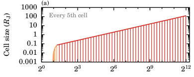
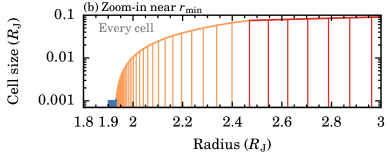
Figure 8: Cell size of the radial grid, from ${r_{\textrm{min}}}=1.9~{}R_{\textrm{J}}$ to ${r_{\textrm{max}}}={R_{\textrm{Hill}}}=4100~{}R_{\textrm{J}}$ in the fiducial case, with its uniform (blue), geometrically stretched (peach), and logarithmic (red) segments. (a) Global view. The central position of only every 5th cell is shown (vertical lines). (b) Zoom-in near ${r_{\textrm{min}}}$. Every cell centre is shown.

Appendix B Dependence of the CPD surface flow on the resolution in the polar direction

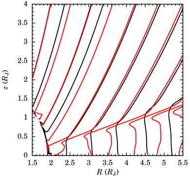
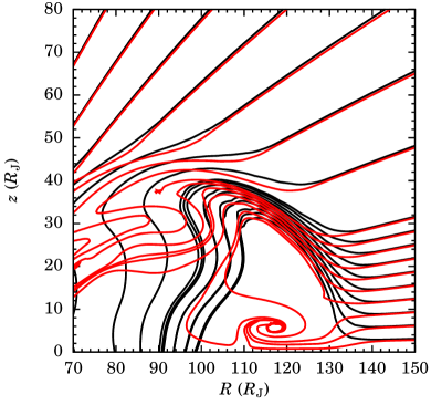
Figure 9: Streamlines for simulations at two $\theta$ resolutions: $\Delta\theta=0.5$° (fiducial run; red) and $\Delta\theta=1.8$° (black). The density structure (essentially the same for both) is shown in Figure 1. In each panel, the $\theta_{\textrm{init}}=\theta({r_{\textrm{max}}})$ values of the streamlines are the same for both simulations. Each panel focuses on a different region at a different scale. The flow beneath the CPD shock depends qualitatively on the resolution in the polar direction but this does not affect our results.

Beneath the shock on the CPD surface, in which the polar component of the velocity goes from super- to subsonic, there is a thin layer of $\approx 1$° in which the gas is radially still supersonic. This layered accretion is described in Tanigawa et al. (2012) and seen also by Takasao et al. (2021). In their simulations, the layer, which is resolved, is however much thicker and of order of 15°. We discussed this in Section 5.2.

With our fiducial resolution of ${N_{\theta}}=181$, we obtain layered accretion and outward-directed “backflows” in the layer right below the shock (Tanigawa et al., 2012; Takasao et al., 2021), in which $v_{\theta}$ is subsonic but $v_{r}$ still supersonic (see Figure 9). With ${N_{\theta}}=51$, the gas settles vertically directly to the midplane instead of performing a “U-turn” in a thin layer beforehand. However, the fully supersonic part of the flow, especially close to the planet, is independent of the resolution, and the H $\alpha$ emission also does not depend on the resolution.

Finally, we see that the behaviour of the gas at the outer edge depends somewhat on the resolution. For ${N_{\theta}}=181$, the streamlines within about 4° of the midplane flow downwards, while the others are lifted up (Figure 1b). At ${N_{\theta}}=51$, all streamlines are lifted up. Also, at the outer edge of the CPD, the streamlines are lifted up at the outer edge of the CPD in the ${N_{\theta}}=181$ but not the ${N_{\theta}}=51$ simulation.

Appendix C Variations in the flow pattern

Ideally, we would be able to wait for a quasi-steady state to establish in the flow at large and small scales, and measure from this the different properties ($\dot{M}_{\textrm{H}\,\alpha}$, etc.). In practice, despite months of wall-clock run-time, in the fiducial simulation a density wave was still travelling out in Phase I (as mentioned in Section 3.2.4). It is associated with the growing CPD outer radius and reflects our set-up in which we let the simulation begin without a CPD. This wave changes somewhat the angular distribution of the mass infall close to the freeze radius and thus, in principle, close to the shock radius for Phase II.

We assess how much variation in the H $\alpha$-generating accretion rate could come from this wave. For this, we measure as a function of time the mass flux in the supersonic region within 45° of the pole at a distance of $r=15$, 20, 30, and 50 $R_{\textrm{J}}$ from the planet. Since the flow is smooth, these partial accretion rates will correlate directly with $\dot{M}_{\textrm{H}\,\alpha}$, which is not accessible in Phase I because the freeze radius ${r_{\textrm{frz}}}$ is farther out than the maximal radius for H $\alpha$ generation. Furthermore, since even after $t=900~{}{t_{\textrm{ff,\,glob}}}$ the density wave has not yet reached ${r_{\textrm{max}}}$ but rather is still moving out, we look at simulations with different parameters in which the evolution happens more quickly.

We find that in a simulation with identical parameters but a surface density increased by a factor of ten, large-scale oscillations begin around $700~{}{t_{\textrm{ff,\,glob}}}$. The maximum mass flux is $\dot{M}=10^{-5}~{}M_{\textrm{J}}\,\textrm{yr}^{-1}$ at $r=50~{}R_{\textrm{J}}$ and goes smoothly as a power law down to $5\times 10^{-6}~{}M_{\textrm{J}}\,\textrm{yr}^{-1}$ at $15~{}R_{\textrm{J}}$. The minimum mass flux decreases more steeply from $\dot{M}=2\times 10^{-7}~{}M_{\textrm{J}}\,\textrm{yr}^{-1}$ at $r=50~{}R_{\textrm{J}}$ to $2\times 10^{-8}~{}M_{\textrm{J}}\,\textrm{yr}^{-1}$ at $15~{}R_{\textrm{J}}$. The total influx at ${R_{\textrm{Hill}}}$ is $\dot{M}_{\textrm{Hill,\,net}}=7\times 10^{-5}~{}M_{\textrm{J}}\,\textrm{yr}^{-1}$ at all times. Therefore, extrapolating down to a radial distance of $r\approx 2~{}R_{\textrm{J}}$, the planet-reaching or H $\alpha$-generating accretion rate is in the range of $0.05$ to $\sim 10^{-5}$ times $\dot{M}_{\textrm{Hill,\,net}}$. The minimum value has a considerable uncertainty due to the extrapolation. These are partial rates and are integrated in angle only down to 45° from the pole but the correction down to the CPD height would not be too large. Assuming that these relative numbers are independent of the surface density and thus also apply to the fiducial run, we would obtain $\dot{M}_{\textrm{p,\,direct}}$ or $\dot{M}_{\textrm{H}\,\alpha}$ values only up to a factor $\approx 20$ larger than what we found in the fiducial run (see Figure 4b) if we let Phase II begin from a different moment of Phase I. At the other extreme, the partial mass fluxes could be orders of magnitude smaller than what we found.

The upshot of this estimate is that there are transient oscillations but they will not affect the basic and crucial point that only a fraction, clearly below 100 %, of the gas falling onto the CPD can generate emission lines.

Appendix D Temperature and luminosity structure

Figure 10 shows the temperature near the planet surface, and Figure 11 the velocity, temperature, fluxes, and angular frequency along two cuts. In Figure 10, the shocks on the planet and the CPD surfaces are clearly visible as Zel’dovich spikes (Zel’dovich & Raizer, 1967; see also discussion in Paper II). Thanks to the small cell sizes (see Figure 8), they reach respectively $T>25000$ K and $T>4000$ K, off the colourscale (capped at 3000 K), but this is resolution-dependent. The true physical peak temperature would be of order $10^{4}$–$10^{5}$ K (Aoyama et al., 2018). Fortunately, this need not be resolved to follow the radiation transfer correctly (Paper II). The pre- and postshock temperatures, which set more directly the thermal structure of the accretion flow and the settling layers below the shock, are equal and near $T=1100$ K.

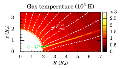
Figure 10: Temperature close to the planet. The colour scale is capped at 3000 K but the Zel’dovich spikes—the extremely thin bright regions above the planetary surface and the CPD surface—as well as the innermost hydrostatic parts near ${r_{\textrm{min}}}$ reach much higher temperatures. Streamlines for the bolometric radiation are shown (dashed white lines), whereas hydrogen lines, including H $\alpha$, originate from both shocks (see regions with a non-grey preshock velocity in Figure 2). The radial segment at $\theta=77$° (green) is analysed in Figure 11 and compared to a vertical segment at $R=2.5~{}R_{\textrm{J}}$.

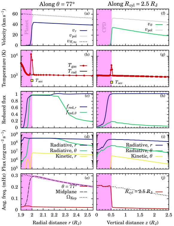
Figure 11: One-dimensional cuts along a line of constant angle $\theta=77$° (left column; corresponding to the green line segment in Figure 10, just above the CPD surface) and of constant cylindrical radius $R=2.5~{}R_{\textrm{J}}$ (right column) in the ${N_{\theta}}=181$ simulation. In the pink regions, the gas is in hydrostatic equilibrium. (a/f) Radial $v_{r}$, total poloidal ${v_{\textrm{pol}}}$, and free-fall velocities ${v_{\textrm{ff},\,\infty}}$; (b/g) gas and radiation temperatures, showing in (b) the radial zoning, and with ${T_{\textrm{acc}}}$; (c/h) reduced flux in $r$ and in $\theta$; (d/i) bolometric radiative flux ${F_{\textrm{rad},\,x}}$ and mechanical ${F_{\textrm{kin},\,x}}=0.5\rho|v_{x}|^{3}$ in direction $x=r$ or $x=\theta$, corresponding to ${T_{\textrm{acc}}}$; and (e/j) angular frequency $\Omega=v_{\phi}/R$ compared to the Keplerian frequency ${\Omega_{\textrm{Kep}}}$. Panel (e) also shows $\Omega$ in the midplane (dashed), which is in (rotation-modified) hydrostatic equilibrium in $R$ and $z$ out to the CPD outer edge (not shown). The apparent steps in the right column are a plotting artefact.

Below the CPD surface shock, the temperature is nearly constant (except close to the midplane), which reflects the low opacity. Nevertheless, the polar reduced flux,

$${f_{\textrm{red},\,\theta}}\equiv\frac{|{F_{\textrm{rad},\,\theta}}|}{c{E_{\textrm{rad}}}},$$ (D1)

where ${F_{\textrm{rad},\,\theta}}$ is the radiation flux in the polar direction, is at most ${f_{\textrm{red},\,\theta}}\approx 0.1$, while the radial reduced flux ${f_{\textrm{red},\,r}}$ goes smoothly from ${f_{\textrm{red},\,r}}=0.01$–0.1 near the midplane to ${f_{\textrm{red},\,r}}=1$ below, at, and above the CPD surface shock. Thus the radiation diffuses in the polar direction while also diffusing radially (below the CPD shock) or flowing freely (above it).

The temperature at the shock on the planet surface is $T_{\textrm{shock}}\approx 1150$ K. This however is set mostly by the luminosity below the shock coming from the compression of the gas. Namely, the free-streaming “accretion temperature” for an $\eta^{\rm kin}=100$ % shock efficiency (Paper I), given by

$$\sigma_{\textrm{SB}}{T_{\textrm{acc}}}^{4}={F_{\textrm{kin},\,r}}=\frac{1}{2}\rho{|v_{r}|}^{3},$$ (D2)

where $\sigma_{\textrm{SB}}$ is the Stefan–Boltzmann constant, is only ${T_{\textrm{acc}}}=615$ K at $\theta=77$° or ${T_{\textrm{acc}}}=715$ K at the pole. In both cases this is much smaller than $T_{\textrm{shock}}$. (This is the limit $\ell=1$ of Equation (33) in Paper II, while here $\ell\gg 1$ since the downstream luminosity dominates.) In the classical assumption of pure radial infall, the direct-infall $\dot{M}_{\textrm{p,\,direct}}$ would be predicted to lead to an accretion temperature ${T^{\prime}_{\textrm{acc}}}=(GM_{\textrm{p}}\dot{M}_{\textrm{p,\,direct}}/[4\pi R_{\textrm{p}}^{3}\sigma_{\textrm{SB}}])^{1/4}=684$ K, ignoring here a factor $f_{\textrm{fill}}/\zeta$ (Zhu, 2015), of order unity. As it should, ${T^{\prime}_{\textrm{acc}}}$ lies between the pole and equator values for ${T_{\textrm{acc}}}$. However, the pendant to this (from a global-simulation point of view) is implicitly to assume that the entire mass flux $\dot{M}_{\textrm{Hill,\,net}}$ shocks on the planetary surface, leading to ${T_{\textrm{acc,\,class}}}=2665$ K, which would dominate the interior luminosity. Neither this radiation temperature ${T_{\textrm{acc,\,class}}}$ nor the corresponding gas temperature in the free-streaming limit $T={T_{\textrm{acc,\,class}}}/4^{1/4}$ have any relevance in describing the system: the gas falls in more slowly and spread over a much larger area than assumed by the formula.

On the surface of the CPD at $R=2.5~{}R_{\textrm{J}}$, the temperature is $T=1070$ K, with the actual ${T_{\textrm{acc}}}=505$ K again much smaller in terms of the radiation fluxes $F\propto T^{4}$ (the gas and radiation temperatures are equal). Thus also for the CPD, it is the interior luminosity, not the kinetic energy of the gas, that is responsible for setting the temperature.

In the midplane there is no shock at the planet surface. Instead, the planet and CPD are connected by a boundary layer (e.g., Hertfelder & Kley, 2017; Dong et al., 2021) in which the angular velocity in the midplane peaks, somewhat above the Keplerian value ${\Omega_{\textrm{Kep}}}=\sqrt{GM_{\textrm{p}}/r^{3}}$, before decreasing smoothly to join the boundary condition at ${r_{\textrm{min}}}$ (Figure 11e). This region will not be studied further here. At least at $R=2.5~{}R_{\textrm{J}}$, the whole vertical extent of the CPD is in Keplerian rotation: in the pink regions in Figure 11j, $\Omega={\Omega_{\textrm{Kep}}}$. The boundary layer leads to a higher temperature close to the midplane but only slightly so.

Away from the CPD (for $r\gtrsim 100~{}R_{\textrm{J}}$), the temperature distribution is independent of polar angle, with temperatures below 100 K. In that regime, the dust opacity $\kappa_{\textrm{dust,\,Ross}}\approx 0.01~{}\textrm{cm}^{2}\,\textrm{g}^{-1}$ dominates by 3–4 dex over the gas opacity even for our choice of a low $f_{\textrm{d/g}}=10^{-4}$. The radial Rosseland optical depth from ${r_{\textrm{max}}}$ to the shock is $\Delta\tau_{\textrm{Ross}}\sim 3\times 10^{-3}$ along the pole, roughly a factor of two higher on a path just above the CPD, and $\Delta\tau_{\textrm{Ross}}=10^{-3}$ in the midplane down to the outer edge of the CPD. The low overall optical depth reflects the low $f_{\textrm{d/g}}$ and modest mass inflow into the Hill sphere $\dot{M}_{\textrm{Hill,\,net}}\sim 10^{-5}~{}M_{\textrm{J}}\,\textrm{yr}^{-1}$ (Table 2).

In this particular example, most of the bolometric flux reaching the observer is coming from the interior of the planet and from the CPD itself. These fluxes do not come from the immediate conversion of kinetic energy but rather from the cooling of the hydrostatic regions below the shocks. This in turn depends on the accretion history. In a given simulation, this history is set by the numerical approach (here, the two-phase system we used, which spans several free-fall timescales), and in general by the variation of the accretion rate over formation timescales of order 1 Myr.

In Section 5.1, we compared the H $\alpha$ flux that we predict to the observed one for PDS 70 b. Assuming, roughly, a linear scaling of the H $\alpha$ luminosity with the mass inflow rate, the latter would need to be 7–100 times larger than in our simulation in order to match the observed $L_{\textrm{H}\,\alpha}$. From Equation (D2), this would imply ${T_{\textrm{acc}}}\approx 1000$–1900 K at the planet’s surface near the CPD, and up to ${T_{\textrm{acc}}}\approx 2300$ K at the pole. In this case, the accretion luminosity from the shock would likely dominate the temperature structure, and the highest accretion rates would be more challenging to reconcile with the constraints from Wang et al. (2021) on $T_{\textrm{eff}}$ from the $K$-band spectral shape. Details such as the viewing geometry or complex radiation-transfer effects could however play an important role. Next-generation spectroscopic observations would be helpful to develop a robust and self-consistent picture.

References

- Adams & Batygin (2022) Adams, F. C., & Batygin, K. 2022, ApJ, 934, 111
- Aoyama et al. (2018) Aoyama, Y., Ikoma, M., & Tanigawa, T. 2018, ApJ, 866, 84
- Aoyama et al. (2021) Aoyama, Y., Marleau, G.-D., Ikoma, M., & Mordasini, C. 2021, ApJ, 917, L30
- Aoyama et al. (2020) Aoyama, Y., Marleau, G.-D., Mordasini, C., & Ikoma, M. 2020, arXiv e-prints, arXiv:2011.06608
- Asensio-Torres et al. (2021) Asensio-Torres, R., Henning, T., Cantalloube, F., et al. 2021, A&A, 652, A101
- Ayliffe & Bate (2009a) Ayliffe, B. A., & Bate, M. R. 2009a, MNRAS, 393, 49
- Ayliffe & Bate (2009b) Ayliffe, B. A., & Bate, M. R. 2009b, MNRAS, 397, 657
- Ayliffe & Bate (2012) Ayliffe, B. A., & Bate, M. R. 2012, MNRAS, 427, 2597
- Bae et al. (2019) Bae, J., Zhu, Z., Baruteau, C., et al. 2019, ApJ, 884, L41
- Bailey et al. (2021) Bailey, A., Stone, J. M., & Fung, J. 2021, ApJ, 915, 113
- Batygin (2018) Batygin, K. 2018, AJ, 155, 178
- Berardo et al. (2017) Berardo, D., Cumming, A., & Marleau, G.-D. 2017, ApJ, 834, 149
- Béthune & Rafikov (2019a) Béthune, W., & Rafikov, R. R. 2019a, MNRAS, 487, 2319
- Béthune & Rafikov (2019b) Béthune, W., & Rafikov, R. R. 2019b, MNRAS, 488, 2365
- Betti et al. (2022a) Betti, S. K., Follette, K. B., Ward-Duong, K., et al. 2022a, ApJ, 935, L18
- Betti et al. (2022b) Betti, S. K., Follette, K. B., Ward-Duong, K., et al. 2022b, ApJ, 941, L20
- Bodenheimer et al. (2000) Bodenheimer, P., Hubickyj, O., & Lissauer, J. J. 2000, Icarus, 143, 2
- Bonse et al. (2023) Bonse, M. J., Garvin, E. O., Gebhard, T. D., et al. 2023, arXiv e-prints, arXiv:2303.12030
- Brittain et al. (2020) Brittain, S. D., Najita, J. R., Dong, R., & Zhu, Z. 2020, ApJ, 895, 48
- Bryan et al. (2018) Bryan, M. L., Benneke, B., Knutson, H. A., Batygin, K., & Bowler, B. P. 2018, NatAs, 2, 138
- Bryan et al. (2020) Bryan, M. L., Ginzburg, S., Chiang, E., et al. 2020, ApJ, 905, 37
- Chachan et al. (2021) Chachan, Y., Lee, E. J., & Knutson, H. A. 2021, ApJ, 919, 63
- Chazelas et al. (2020) Chazelas, B., Lovis, C., Blind, N., et al. 2020, in Society of Photo-Optical Instrumentation Engineers (SPIE) Conference Series, Vol. 11448, Society of Photo-Optical Instrumentation Engineers (SPIE) Conference Series, 1144875
- Chen & Bai (2022) Chen, Z., & Bai, X. 2022, ApJ, 925, L14
- Choksi et al. (2023) Choksi, N., Chiang, E., Fung, J., & Zhu, Z. 2023, arXiv e-prints, arXiv:2305.01684
- Christensen et al. (2009) Christensen, U. R., Holzwarth, V., & Reiners, A. 2009, Nature, 457, 167
- Cimerman et al. (2017) Cimerman, N. P., Kuiper, R., & Ormel, C. W. 2017, MNRAS, 471, 4662
- Close (2020) Close, L. M. 2020, AJ, 160, 221
- Cugno et al. (2019) Cugno, G., Quanz, S. P., Hunziker, S., et al. 2019, A&A, 622, A156
- Currie et al. (2022) Currie, T., Lawson, K., Schneider, G., et al. 2022, NatAs, 6, 751
- Delorme et al. (2021) Delorme, J.-R., Jovanovic, N., Echeverri, D., et al. 2021, Journal of Astronomical Telescopes, Instruments, and Systems, 7, 035006
- Dong et al. (2021) Dong, J., Jiang, Y.-F., & Armitage, P. J. 2021, ApJ, 921, 54
- Dong et al. (in prep.) Dong, R., Hashimoto, J., Haffert, S., et al. in prep., ApJ
- Drążkowska et al. (2019) Drążkowska, J., Li, S., Birnstiel, T., Stammler, S. M., & Li, H. 2019, ApJ, 885, 91
- Emsenhuber et al. (2021) Emsenhuber, A., Mordasini, C., Burn, R., et al. 2021, A&A, 656, A69
- Eriksson et al. (2020) Eriksson, S. C., Asensio Torres, R., Janson, M., et al. 2020, A&A, 638, L6
- Follette et al. (2023) Follette, K. B., Close, L. M., Males, J. R., et al. 2023, AJ, 165, 225
- Fu et al. (2023) Fu, Z., Huang, S., & Yu, C. 2023, ApJ, 945, 165
- Fung et al. (2019) Fung, J., Zhu, Z., & Chiang, E. 2019, ApJ, 887, 152
- Goldreich & Lynden-Bell (1965) Goldreich, P., & Lynden-Bell, D. 1965, MNRAS, 130, 125
- Haffert et al. (2019) Haffert, S. Y., Bohn, A. J., de Boer, J., et al. 2019, NatAs, 3, 749
- Haffert et al. (2021) Haffert, S. Y., Males, J. R., Close, L., et al. 2021, in Society of Photo-Optical Instrumentation Engineers (SPIE) Conference Series, Vol. 11823, Techniques and Instrumentation for Detection of Exoplanets X, ed. S. B. Shaklan & G. J. Ruane, 1182306
- Hartmann et al. (1997) Hartmann, L., Cassen, P., & Kenyon, S. J. 1997, ApJ, 475, 770
- Hartmann et al. (2016) Hartmann, L., Herczeg, G., & Calvet, N. 2016, ARA&A, 54, 135
- Hasegawa et al. (2021) Hasegawa, Y., Kanagawa, K. D., & Turner, N. J. 2021, ApJ, 923, 27
- Hertfelder & Kley (2017) Hertfelder, M., & Kley, W. 2017, A&A, 605, A24
- Hill (1878) Hill, G. W. 1878, AmJM, 1, 5
- Huélamo et al. (2022) Huélamo, N., Chauvin, G., Mendigutía, I., et al. 2022, A&A, 668, A138
- Isella & Natta (2005) Isella, A., & Natta, A. 2005, A&A, 438, 899
- Kanagawa et al. (2017) Kanagawa, K. D., Tanaka, H., Muto, T., & Tanigawa, T. 2017, PASJ, 69, 97
- Kanagawa et al. (2018) Kanagawa, K. D., Tanaka, H., & Szuszkiewicz, E. 2018, ApJ, 861, 140
- Karlin et al. (2023) Karlin, S. M., Panić, O., & van Loo, S. 2023, MNRAS, 520, 1258
- Katarzyński et al. (2016) Katarzyński, K., Gawroński, M., & Goździewski, K. 2016, MNRAS, 461, 929
- Keith & Wardle (2014) Keith, S. L., & Wardle, M. 2014, MNRAS, 440, 89
- Keppler et al. (2018) Keppler, M., Benisty, M., Müller, A., et al. 2018, A&A, 617, A44
- Kley (1989) Kley, W. 1989, A&A, 208, 98
- Kley (1998) Kley, W. 1998, A&A, 338, L37
- Korycansky & Papaloizou (1996) Korycansky, D. G., & Papaloizou, J. C. B. 1996, ApJS, 105, 181
- Krapp et al. (2022) Krapp, L., Kratter, K. M., & Youdin, A. N. 2022, ApJ, 928, 156
- Kuiper et al. (2010) Kuiper, R., Klahr, H., Dullemond, C., Kley, W., & Henning, T. 2010, A&A, 511, A81
- Kuiper et al. (2020) Kuiper, R., Yorke, H. W., & Mignone, A. 2020, ApJS, 250, 13
- Kurokawa & Tanigawa (2018) Kurokawa, H., & Tanigawa, T. 2018, MNRAS, 479, 635
- Lambrechts & Lega (2017) Lambrechts, M., & Lega, E. 2017, A&A, 606, A146
- Lambrechts et al. (2019) Lambrechts, M., Lega, E., Nelson, R. P., Crida, A., & Morbidelli, A. 2019, A&A, 630, A82
- Lovelace et al. (2011) Lovelace, R. V. E., Covey, K. R., & Lloyd, J. P. 2011, AJ, 141, 51
- Machida et al. (2008) Machida, M. N., Kokubo, E., Inutsuka, S.-i., & Matsumoto, T. 2008, ApJ, 685, 1220
- Maeda et al. (2022) Maeda, N., Ohtsuki, K., Tanigawa, T., Machida, M. N., & Suetsugu, R. 2022, ApJ, 935, 56
- Mai et al. (2020) Mai, C., Desch, S. J., Kuiper, R., Marleau, G.-D., & Dullemond, C. 2020, ApJ, 899, 54
- Malygin et al. (2014) Malygin, M. G., Kuiper, R., Klahr, H., Dullemond, C. P., & Henning, T. 2014, A&A, 568, A91
- Marleau et al. (2017) Marleau, G.-D., Klahr, H., Kuiper, R., & Mordasini, C. 2017, ApJ, 836, 221
- Marleau et al. (2019) Marleau, G.-D., Mordasini, C., & Kuiper, R. 2019, ApJ, 881, 144
- Marleau et al. (2022) Marleau, G.-D., Aoyama, Y., Kuiper, R., et al. 2022, A&A, 657, A38
- Marley et al. (2007) Marley, M. S., Fortney, J. J., Hubickyj, O., Bodenheimer, P., & Lissauer, J. J. 2007, ApJ, 655, 541
- Marois et al. (2008) Marois, C., Lafrenière, D., Macintosh, B., & Doyon, R. 2008, ApJ, 673, 647
- Mendoza et al. (2009) Mendoza, S., Tejeda, E., & Nagel, E. 2009, MNRAS, 393, 579
- Mignone et al. (2007) Mignone, A., Bodo, G., Massaglia, S., et al. 2007, ApJS, 170, 228
- Mignone et al. (2012) Mignone, A., Zanni, C., Tzeferacos, P., et al. 2012, ApJS, 198, 7
- Moldenhauer et al. (2021) Moldenhauer, T. W., Kuiper, R., Kley, W., & Ormel, C. W. 2021, A&A, 646, L11
- Moldenhauer et al. (2022) Moldenhauer, T. W., Kuiper, R., Kley, W., & Ormel, C. W. 2022, A&A, 661, A142
- Mordasini (2013) Mordasini, C. 2013, A&A, 558, A113
- Mordasini et al. (2012a) Mordasini, C., Alibert, Y., Georgy, C., et al. 2012a, A&A, 547, A112
- Mordasini et al. (2012b) Mordasini, C., Alibert, Y., Klahr, H., & Henning, T. 2012b, A&A, 547, A111
- Müller et al. (2018) Müller, A., Keppler, M., Henning, T., et al. 2018, A&A, 617, L2
- Mungan (2009) Mungan, C. E. 2009, The Physics Teacher, 47, 502
- Nelson et al. (2023) Nelson, R. P., Lega, E., & Morbidelli, A. 2023, A&A, 670, A113
- Nielsen et al. (2019) Nielsen, E. L., De Rosa, R. J., Macintosh, B., et al. 2019, AJ, 158, 13
- Paxton et al. (2019) Paxton, B., Smolec, R., Schwab, J., et al. 2019, ApJS, 243, 10
- Pringle (1981) Pringle, J. E. 1981, ARA&A, 19, 137
- Ringqvist et al. (2023) Ringqvist, S. C., Viswanath, G., Aoyama, Y., et al. 2023, A&A, 669, L12
- Romanova et al. (2002) Romanova, M. M., Ustyugova, G. V., Koldoba, A. V., & Lovelace, R. V. E. 2002, ApJ, 578, 420
- Sanchis et al. (2020) Sanchis, E., Picogna, G., Ercolano, B., Testi, L., & Rosotti, G. 2020, MNRAS, 492, 3440
- Sanghi et al. (2022) Sanghi, A., Zhou, Y., & Bowler, B. P. 2022, AJ, 163, 119
- Schulik et al. (2019) Schulik, M., Johansen, A., Bitsch, B., & Lega, E. 2019, A&A, 632, A118
- Schulik et al. (2020) Schulik, M., Johansen, A., Bitsch, B., Lega, E., & Lambrechts, M. 2020, A&A, 642, A187
- Semenov et al. (2003) Semenov, D., Henning, T., Helling, C., Ilgner, M., & Sedlmayr, E. 2003, A&A, 410, 611
- Shakura & Sunyaev (1973) Shakura, N. I., & Sunyaev, R. A. 1973, A&A, 500, 33
- Stolker et al. (2020) Stolker, T., Marleau, G. D., Cugno, G., et al. 2020, A&A, 644, A13
- Szulágyi (2017) Szulágyi, J. 2017, ApJ, 842, 103
- Szulágyi et al. (2022) Szulágyi, J., Binkert, F., & Surville, C. 2022, ApJ, 924, 1
- Szulágyi et al. (2019) Szulágyi, J., Dullemond, C. P., Pohl, A., & Quanz, S. P. 2019, MNRAS, 487, 1248