Stress and heat flux via automatic differentiation

Abstract

Machine-learning potentials provide computationally efficient and accurate approximations of the Born-Oppenheimer potential energy surface. This potential determines many materials properties and simulation techniques usually require its gradients, in particular forces and stress for molecular dynamics, and heat flux for thermal transport properties. Recently developed potentials feature high body order and can include equivariant semi-local interactions through message-passing mechanisms. Due to their complex functional forms, they rely on automatic differentiation (AD), overcoming the need for manual implementations or finite-difference schemes to evaluate gradients. This study demonstrates a unified AD approach to obtain forces, stress, and heat flux for such potentials, and provides a model-independent implementation. The method is tested on the Lennard-Jones potential, and then applied to predict cohesive properties and thermal conductivity of tin selenide using an equivariant message-passing neural network potential.

I Introduction

Molecular dynamics (MD) simulations enable computational prediction of thermodynamic quantities for a wide range of quantum systems, and constitute a cornerstone of modern computational science Tuckerman (2010). In MD, systems are simulated by propagating Newton’s equations of motion – potentially modified to model statistical ensembles – numerically in time, based on the forces acting on each atom due to their movement on the Born-Oppenheimer potential-energy surface (PES). Therefore, the quality of the underlying PES is important for the predictive ability of this method. First-principles electronic structure methods such as density-functional theory (DFT) can be used to perform high-accuracy MD simulations Car and Parrinello (1985), provided the exchange-correlation approximation is reliable Teale et al. (2022). Such approaches are, however, restricted by high computational cost, severely limiting accessible size and time scales. Computationally efficient approximations to the underlying PES are therefore required for the atomistic simulation of larger systems: Forcefields (FFs) are built on analytical functional forms that are often based on physical bonding principles, parametrized to reproduce quantities of interest for a given material González (2011). They are computationally cheap, but parametrizations for novel materials are not always available, and their flexibility is limited by their fixed functional form. Machine-learning potentials (MLPs) Lorenz, Groß, and Scheffler (2004); Li et al. (2006); Behler and Parrinello (2007); Bartók et al. (2010); Lorenz, Groß, and Scheffler (2004); Behler and Parrinello (2007); Chmiela et al. (2018, 2019); Poltavsky and Tkatchenko (2021), where a potential is inferred based on a small set of reference calculations, aim to retain near first-principles accuracy while remaining linear scaling with the number of atoms. While MLPs are limited, in principle, to modeling the physical mechanisms present in the training data, they have nevertheless emerged as an important tool for MD Noé et al. (2020); Unke et al. (2020); Keith et al. (2021); Unke et al. (2021a, 2022), often combined with active learning schemes Csányi et al. (2004); Jinnouchi et al. (2020); Verdi et al. (2021); van der Oord et al. (2022); Xie et al. (2022). Modern MLPs can include semi-local interactions through message-passing (MP) mechanisms Gilmer et al. (2017), internal equivariant representations Thomas et al. (2018), and body-order expansions Drautz (2019), which enable the efficient construction of flexible many-body interactions. In such complex architectures, the manual implementation of derivatives is often unfeasible. Finite-difference approaches require tuning of additional parameters, as well as repeated energy evaluations. Automatic differentiation (AD) Griewank and Walther (2008); Baydin et al. (2017) presents an intriguing alternative: If the computation of the potential energy $U$ is implemented in a suitable framework, derivatives such as the forces $\bm{F}$ or the stress $\bm{\sigma}$ can be computed with the same asymptotic computational cost as computing the energy. This is accomplished by decomposing the underlying ‘forward’ computation into elementary operations with analytically tractable derivatives, computing local gradients for a given input, and then combining the resulting values using the chain rule.

This work provides a systematic discussion of the use of AD to compute forces, stress, and heat flux for MLPs. While the calculation of forces with AD is common practice Schoenholz and Cubuk (2020); Schütt et al. (2018a); Unke and Meuwly (2019); Schütt et al. (2023), stress and heat flux are not yet commonly available for many MLPs. Both quantities have been the focus of much previous work due to the difficulty of defining and implementing them for many-body potentials and periodic boundary conditions Louwerse and Baerends (2006); Torii, Nakano, and Ohara (2008); Thompson, Plimpton, and Mattson (2009); Volz and Chen (1999); Chen (2006); Guajardo-Cuéllar, Go, and Sen (2010); Fan et al. (2015); Marcolongo, Umari, and Baroni (2015); Carbogno, Ramprasad, and Scheffler (2017); Boone, Babaei, and Wilmer (2019); Surblys et al. (2019); Langer et al. (2023). Introducing an abstract definition of MLPs as functions of a graph representation of atomistic systems, unified formulations of stress and heat flux are given, which can be implemented generally for any such graph-based machine-learning potential (GLP). An example implementation using jax Bradbury et al. (2018) is provided in the glp package Langer (2023). To validate the approach, different formulations of stress and heat flux are compared for the Lennard-Jones potential Lennard-Jones (1924), where analytical derivatives are readily available for comparison, as well as a state-of-the art message-passing neural network (MPNN), so3krates Frank, Unke, and Müller (2022). Having established the correctness of the proposed implementation, the ability of so3krates to reproduce first-principles cohesive properties and thermal conductivity of tin selenide (SnSe) is studied.

II Automatic Differentiation

Automatic differentiation (AD) is a technique to obtain derivatives of functions implemented as computer programs. Griewank and Walther (2008); Baydin et al. (2017) It is distinct from numerical differentiation, where finite-difference schemes are employed, and symbolic differentiation, where analytical derivatives are obtained manually or via computer algebra systems, and then implemented explicitly. Instead, AD relies on the observation that complex computations can often be split up into elementary steps, for which derivatives are readily implemented. If one can track those derivatives during the computation of the forward, or ‘primal’, function, the chain rule allows to obtain derivatives.

For this work, two properties of AD are particularly relevant: It allows the computation of derivatives with respect to quantities that are explicitly used in the forward computation, and it can do so at the same asymptotic computational cost as the forward function. In particular, AD can obtain two quantities efficiently: Given a differentiable function $u:\mathbb{R}^{N}\rightarrow\mathbb{R}^{M}$, the Jacobian of $u$ is defined as the $M\times N$ matrix $\partial u_{i}(\bm{x})/\partial x_{j}$. AD can then obtain Jacobian-vector and vector-Jacobian products, i.e., the multiplication and summation of factors over either the input or the output dimension. This corresponds to propagating derivatives from the inputs forwards, leading to forward-mode AD, or from the end result backwards, leading to reverse-mode AD. As many popular AD frameworks are primarily implemented to work with neural networks, where scalar loss functions must be differentiated with respect to many parameters, reverse-mode AD, also called ‘backpropagation’, Rumelhart, Hinton, and Williams (1986) is more generally available. More recent frameworks implement both approaches, for instance jax Bradbury et al. (2018) which is used in the present work. AD can also be leveraged to compute contractions of higher-order derivative operators Schmitz, Müller, and Chmiela (2022).

III Constructing Graph MLPs

This work considers periodic systems, consisting of $N$ atoms with atomic numbers $Z_{i}$ placed in a simulation cell which is infinitely periodically tiled in space. We define

$$\mathrm{R_{\text{sc}}} \coloneqq\{\,\bm{r}_{i}\,:\,i=1...N\,\}$$ positions in simulation cell

$$\mathrm{Z} \coloneqq\{\,Z_{i}\,:\,i=1...N\,\}$$ atomic numbers

$$\mathrm{B} \coloneqq\{\,\bm{b}_{a}\,:\,a=1,2,3\,\}$$ basis or lattice vectors

$$\bm{r}_{i\bm{n}} \coloneqq\bm{r}_{i}+\sum_{a}\nolimits n_{a}\bm{b}_{a}$$ (replica) position

$$\mathrm{R_{\text{all}}} \coloneqq\{\,\bm{r}_{i\bm{n}}\,:\,\bm{r}_{i}\in\mathrm{R_{\text{sc}}},\bm{n}\in\mathbb{Z}^{3}\,\}$$ all (bulk) positions

$$\bm{r}_{ij} \coloneqq\bm{r}_{j}-\bm{r}_{i}$$ atom-pair vector

$$\bigl{|}\bm{r}^{\text{MIC}}_{ij}\bigr{|} \coloneqq\min_{\bm{n}\in\mathbb{Z}^{3}}\bigl{|}\bm{r}_{j}+\sum_{a}n_{a}\bm{b}_{a}-\bm{r}_{i}\bigr{|}$$ minimum image convention

In this setting, a MLP is a function that maps the structure represented by its positions, lattice vectors, and atomic numbers, $(\mathrm{R_{\text{sc}}},\mathrm{B},\mathrm{Z})$, to a set of atomic potential energies $\mathrm{U}\coloneqq\{\,U_{i}\,:\,i=1\,...\,N\,\}$, which yield the total potential energy $U=\sum_{i=1}\nolimits U_{i}$. Since AD relies on the forward computation to calculate derivatives, it is sensitive to the exact implementation of this mapping. Care must therefore be taken to construct the MLP such that required derivatives are available.

This work considers MLPs that scale linearly with $N$. Therefore, the number of atoms contributing to a given $U_{i}$ must be bounded, which is achieved by introducing a cutoff radius $r_{\text{c}}$, restricting interactions to finite-sized atomic neighborhoods $\mathrm{N}(i)=\{\,\bm{r}_{j}\,:\,\bigl{|}\bm{r}_{ij}\bigr{|}\leq r_{\text{c}},\bm{r}_{j}\in\mathrm{R_{\text{all}}}\,\}$. To ensure translational invariance, MLPs do not rely on neighbor positions directly, but rather on atom-pair vectors centered on $i$, from which atom-pair vectors between neighboring atoms can be constructed, for instance to determine angles.

The resulting structure can be seen as a graph $\mathrm{G}$. The vertices $\mathrm{V}$ of this graph are identified with atoms, labeled with their respective atomic numbers, and connected by edges $\mathrm{E}$ that are labeled with atom-pair vectors if placed closer than $r_{\text{c}}$. Starting from $\mathrm{G}$, MLPs can be constructed in different ways: Local MLPs compute a suitable representation Langer, Goeßmann, and Rupp (2022) of each neighborhood, and predict $U_{i}$ from that representation using a learned function, such as a neural network or a kernel machine. Such models are conceptually simple, but cannot account for effects that extend beyond $r_{\text{c}}$. Recently, semi-local models such as MPNNs Gilmer et al. (2017); Schütt et al. (2017, 2018b); Unke and Meuwly (2019); Klicpera, Groß, and Günnemann (2020); Batzner et al. (2022); Unke et al. (2021b); Batatia et al. (2022a, b); Bochkarev et al. (2022) have been introduced to tackle this shortcoming without compromising asymptotic runtime. In such models, effective longer-range interactions are built up iteratively by allowing adjacent neighborhoods to interact repeatedly. We introduce the parameter $M$, the interaction depth, to quantify how many such iterations are included. After $M$ interactions, the energy at any given site can depend implicitly on positions within $M$ hops on the graph, which we denote by $\mathrm{N}^{M}\!\!(i)$, leading to an effective cutoff radius $r_{\text{c}}^{\text{eff}}=M\,r_{\text{c}}$. However, since interactions are confined to neighborhoods at each iteration, the asymptotic linear scaling is not impacted. Local MLPs are formally included as semi-local models with $M{=}1$, allowing a unified treatment for both. We term this class of potentials, which act on sets of neighborhoods and use atom-pair vectors as input, graph-based machine-learning potentials (GLPs). By construction, this framework does not include global interactions.

We consider two strategies to construct GLPs: The ‘standard’ way, which includes periodic boundary conditions via the edges in the graph, and an ‘unfolded’ formulation, where periodicity is explicitly included via replica positions.

In the standard architecture, vertices in $\mathrm{G}$ are identified with atoms in the simulation cell, using the minimum image convention (MIC) to include periodicity. Edges $\mathrm{E}_{ij}$ exist between two atoms $i$ and $j$ in $\mathrm{R_{\text{sc}}}$ if they interact:

$$\mathrm{E}^{\text{std}}_{ij}=\{\,\bm{r}^{\text{MIC}}_{ij}\,:\,\bigl{|}\bm{r}^{\text{MIC}}_{ij}\bigr{|}\leq r_{\text{c}}\,\}\,.$$ (1)

We denote the the graph constructed in this manner as $\mathrm{G}^{\text{std}}$ and the set of edges $\mathrm{E}^{\text{std}}$.

Alternatively, we can first determine the total set of positions $\mathrm{R_{\text{unf}}}\subset\mathrm{R_{\text{all}}}$ that can interact with atoms in the simulation cell, creating an ‘unfolded’ system extracted from the bulk, consisting of $\mathrm{R_{\text{sc}}}$ and all replicas with up to $r_{\text{c}}^{\text{eff}}$ distance from the cell boundary. This construction can be performed efficiently, and adds only a number of positions that is proportional to the surface of the simulation cell, therefore becoming increasingly negligible as $N$ increases at constant density Langer et al. (2023). We proceed by constructing a correspondingly modified graph $\mathrm{G}^{\text{unf}}$, and compute potential energies for vertices corresponding to atoms in the simulation cell only. By construction, since the same atom-pair vectors appear in the graph, this approach then reproduces the potential energy of the standard method.

IV Derivatives

Having constructed the forward function for a given GLP, we can compute derivatives with respect to its inputs using AD. In this section, we discuss how forces, stress, and heat flux can be computed in this manner, and demonstrate the relationship between different formulations.

IV.1 Forces

For MD, the most relevant quantities are the forces

$$\bm{F}_{i}=-\frac{\partial U}{\partial\bm{r}_{i}}$$ (2)

acting on the atoms in the simulation cell. Since $\mathrm{R_{\text{sc}}}$ are an explicit input, they can be computed directly with AD: $U$ is a scalar, and this therefore is a trivial Jacobian-vector product, which can be computed with the same asymptotic cost as $U$.

An interesting situation arises if pairwise forces are desired. Strictly speaking, in a many-body MLP, where interactions cannot be decomposed into pairwise contributions, such quantities are not well-defined and Newton’s third law is replaced by conservation of momentum, which requires $\sum_{i=1}^{N}\nolimits\bm{F}_{i}=0$. Nevertheless, pairwise forces with an antisymmetric structure can be defined by exploiting the construction of GLPs in terms of atom-pair vectors. In the standard formulation, $U$ is a function of all edges,

$$U=U(\{\,\bm{r}_{ij}\,:\,ij\in\mathrm{E}^{\text{std}}\,\})\,.$$ (3)

Hence, by the chain rule,

$$\bm{F}_{i} =\sum_{j\in\mathrm{N}(i)}\frac{\partial U}{\partial\bm{r}_{ij}}-\frac{\partial U}{\partial\bm{r}_{ji}}$$ (4)

$$\eqqcolon\sum_{j\in\mathrm{N}(i)}\bm{F}_{ij}\,.$$ (5)

The pairwise forces such defined exhibit anti-symmetry, and therefore fulfil Newton’s third law. For $M{=}1$, the local case, this definition reduces to a more standard form Fan et al. (2015)

$$\bm{F}_{ij}=\frac{\partial U_{i}}{\partial\bm{r}_{ij}}-\frac{\partial U_{j}}{\partial\bm{r}_{ji}}\,.$$ (6)

However, for general GLPs with $M{>}1$, this definition includes a sum over all $U_{k}$ that are influenced by a given edge

$$\bm{F}_{ij}=\sum_{k\in\mathrm{N}^{M}\!\!(i)}\frac{\partial U_{k}}{\partial\bm{r}_{ij}}-\frac{\partial U_{k}}{\partial\bm{r}_{ji}}\,,$$ (7)

subverting expectations connecting local potential energies to pairwise forces. We note that this seeming contradiction is a consequence of the combination of the peculiar construction of GLPs and AD: In principle, it is always possible to define extended neighborhoods up to $r_{\text{c}}^{\text{eff}}$, obtaining $U_{i}$ purely as a function of atom-pair vector originating from $i$. However, to construct derivatives with respect to these atom-pair vectors with AD, these extended neighborhoods have to be constructed and included explicitly, therefore negating the computational efficiency gains of a GLP architecture.

IV.2 Stress

The definition of the (potential) stress is Knuth et al. (2015)

$$\bm{\sigma}=\frac{1}{V}\,\frac{\partial U}{\partial\bm{\epsilon}}{\big{|}}_{\bm{\epsilon}=0}\,,$$ (8)

with $U$ denoting the potential energy after a strain transformation with the the $3\times 3$ symmetric tensor $\bm{\epsilon}$

$$\bm{r}\rightarrow(\mathbb{1}+\bm{\epsilon})\cdot\bm{r}\,,$$ (9)

acting on $\mathrm{R_{\text{all}}}$. While computing this derivative for arbitrary potentials and periodic systems has required ‘much effort’ Louwerse and Baerends (2006) in the past Thompson, Plimpton, and Mattson (2009); Admal and Tadmor (2011), it is straightforward with AD.

The simplest approach, followed for instance by schnetpack Schütt et al. (2018c); sch and nequip Batzner et al. (2022); neq , is to inject the strain transformation explicitly into the construction of the GLP. This can be done at different points: One can transform $\mathrm{R_{\text{sc}}}$ and $\mathrm{B}$ before constructing $\mathrm{G}$, directly transform atom-pair vectors, or transform all contributing positions $\mathrm{R_{\text{unf}}}$. Alternatively, as the inner derivative of inputs with respect to $\bm{\epsilon}$ is simply the input, the derivative of $U$ with respect to inputs can be obtained with AD, and the stress computed analytically from the results. This avoids modifying the forward computation of $U$ entirely.

These approaches yield, with $\otimes$ denoting an outer product,

$$V\bm{\sigma} =\frac{\partial U(\mathrm{R_{\text{sc}}},\mathrm{B})}{\partial\bm{\epsilon}}$$ (10)

$$=\frac{\partial U(\mathrm{E})}{\partial\bm{\epsilon}}$$ (11)

$$=\frac{\partial U(\mathrm{R_{\text{unf}}})}{\partial\bm{\epsilon}}$$ (12)

$$=\sum_{i\in\mathrm{R_{\text{sc}}}}\bm{r}_{j}\otimes\frac{\partial U}{\partial\bm{r}_{i}}+\sum_{\bm{b}\in\mathrm{B}}\bm{b}\otimes\frac{\partial U}{\partial\bm{b}}$$ (13)

$$=\sum_{ij\in\mathrm{E}}\bm{r}_{ij}\otimes\frac{\partial U}{\partial\bm{r}_{ij}}$$ (14)

$$=\sum_{i\in\mathrm{R_{\text{unf}}}}\bm{r}_{i}\otimes\frac{\partial U}{\partial\bm{r}_{i}}\,,$$ (15)

recovering previous formulations given by Louwerse and Baerends Louwerse and Baerends (2006) and Thompson Thompson, Plimpton, and Mattson (2009). As seen in Tables 1 and 3, all such forms of the stress are equivalent, provided the strain transformation is applied consistently to all used inputs. In all cases, as $U$ is differentiated with respect to its inputs, asymptotic cost remains linear.

A more complex situation arises if strain derivatives of atomic energies, i.e., atomic stresses

$$\bm{\sigma}_{i}\coloneqq\frac{1}{V}\frac{\partial U_{i}}{\partial\bm{\epsilon}}\hskip 28.45274pti\in\mathrm{R_{\text{sc}}}$$ (16)

are required. Their calculation requires either one backward pass per $U_{i}$, or one forward pass for each entry in $\bm{\epsilon}$. If only reverse-mode AD is available, its evaluation therefore scales quadratically with $N$. Linear scaling is retained with forward mode. For GLPs with $M{=}1$, linear scaling in reverse mode can be recovered by using Eq. 14: Every edge can be uniquely assigned to one $U_{i}$, and therefore the derivatives can be used to construct atomic stresses. For $M{>}1$, this is not possible; similar to the observations of the previous section, atomic stresses take a semi-local form.

IV.3 Heat Flux

Finally, we discuss the heat flux, which is required to compute thermal conductivities with the Green-Kubo (GK) method Green (1952); Kubo (1957); Kubo, Yokota, and Nakajima (1957). It describes how energy flows between atoms, and has been the focus of a large body of previous work Chen (2006); Admal and Tadmor (2011); Torii, Nakano, and Ohara (2008); Fan et al. (2015); Surblys et al. (2019); Boone, Babaei, and Wilmer (2019); Langer et al. (2023).

The fundamental definition of the heat flux for MLPs was originally derived by Hardy Hardy (1963) for periodic quantum systems. It reads Langer et al. (2023)

$$\bm{J}_{\text{full}} =\sum_{\begin{subarray}{c}i\in\mathrm{R_{\text{sc}}}\\ j\in\mathrm{R_{\text{all}}}\end{subarray}}\left(\bm{r}_{ji}\left(\frac{\partial U_{i}}{\partial\bm{r}_{j}}\cdot\bm{v}_{j}\right)\right)+\sum_{i\in\mathrm{R_{\text{sc}}}}E_{i}\bm{v}_{i}$$ (17)

$$\eqqcolon\bm{J}_{\text{pot}}+\bm{J}_{\text{conv}}\,,$$ (18)

where $\bm{v}_{i}$ denote velocities, $m_{i}$ masses, and $E_{i}=U_{i}+1/2m_{i}\bm{v}_{i}^{2}$ is the total energy per atom. Intuitively, the ‘potential’ term $\bm{J}_{\text{pot}}$ describes how the total instantaneous change in $U_{i}$ can be attributed to interactions with other atoms, with energy flowing between them, while the second, ‘convective’, term $\bm{J}_{\text{conv}}$ describes energy being carried the individual atoms. In the present setting, $\bm{J}_{\text{conv}}$ can be computed directly, as $E_{i}$ are available. $\bm{J}_{\text{pot}}$, however, presents a challenge in an AD framework: In principle, $\bm{J}_{\text{pot}}$ could be computed directly, obtaining the required partial derivatives with AD. However, as $\bm{J}_{\text{pot}}$ is neither a Jacobian-vector nor a vector-Jacobian product, this requires repeated evaluations over the input or output dimension. Even when restricting $j\in\mathrm{R_{\text{sc}}}$, which can be achieved by introducing the MIC for $\bm{r}_{ji}$ (see Supp. Mat. for details),

$$\bm{J}_{\text{pot}}^{\text{MIC}}=\sum_{i,j\in\mathrm{R_{\text{sc}}}}\left(\bm{r}^{\text{MIC}}_{ji}\left(\frac{\partial U_{i}}{\partial\bm{r}_{j}}\cdot\bm{v}_{j}\right)\right)\,,$$ (19)

computational cost of a direct implementation with AD scales quadratically with $N$, rendering the system sizes and simulation times required for the GK method inaccessible Langer et al. (2023). We therefore consider approaches that restore linear scaling in the following.

For $M{=}1$, edges can be uniquely assigned to atomic energy contributions as discussed for atomic stresses in Sec. IV.2. In this case

$$\frac{\partial U}{\partial\bm{r}_{ij}}=\sum_{k\in\mathrm{R_{\text{sc}}}}\frac{\partial U_{k}}{\partial\bm{r}_{ij}}=\frac{\partial U_{i}}{\partial\bm{r}_{ij}}=\frac{\partial U_{i}}{\partial\bm{r}_{j}}\,,$$ (20)

so that

$$\bm{J}_{\text{pot}}^{M{=}1}=\sum_{ij\in\mathrm{E}}\left(\bm{r}_{ji}\left(\frac{\partial U}{\partial\bm{r}_{ij}}\cdot\bm{v}_{j}\right)\right)\,,$$ (21)

which requires a single evaluation of reverse-mode AD.

We note that the terms appearing in front of $\bm{v}_{j}$ also appear in the stress in Eq. 14. However, for a given $j$, the pre-factor cannot be identified with the atomic stress as defined in Eq. 16 – the atomic energy being differentiated is not $U_{j}$, but $U_{i}$. The indices can only be exchanged for additive pairwise potentials; this inequivalence was recently corrected in the LAMMPS code Boone, Babaei, and Wilmer (2019).

This approach is not applicable for $M{>}1$, since the relation in Eq. 20 no longer holds, and the mapping between stress contributions and heat flux contributions becomes invalid. By using the unfolded construction, however, linear scaling can be restored regardlessLanger et al. (2023). Introducing auxiliary positions $\bm{r}^{\text{aux}}_{i}$, which are numerically identical to the positions $\bm{r}_{i}$, but not used to compute $U$, and defining the energy barycenter $\bm{B}=\sum_{i\in\mathrm{R_{\text{sc}}}}\nolimits\bm{r}^{\text{aux}}_{i}U_{i}$, the heat flux can be written as

$$\bm{J}_{\text{pot}}^{M{\geq}1} =\sum_{j\in\mathrm{R_{\text{unf}}}}\frac{\partial\bm{B}}{\partial\bm{r}_{j}}\cdot\bm{v}_{j}-\sum_{j\in\mathrm{R_{\text{unf}}}}\left(\bm{r}_{j}\left(\frac{\partial U}{\partial\bm{r}_{j}}\cdot\bm{v}_{j}\right)\right)\,.$$ (22)

The first term requires three reverse-mode evaluations, or one forward-mode evaluation, the latter a single backward- or forward-mode evaluation. Since the overhead introduced by explicitly constructing $\mathrm{R_{\text{unf}}}$ scales as $N^{2/3}$, overall linear scaling is restored, albeit with a pre-factor due to the higher number of positions to be considered.

To summarize, we have introduced two forms of the heat flux that can be implemented efficiently with AD: Equation 21, which applies to GLPs with $M{=}1$, and Eq. 22, which applies for $M{\geq}1$, but introduces some additional overhead. Both are equivalent to the general, quadratically-scaling, form given in Eq. 17, as seen in Tables 2 and 4.

V Experiments

V.1 Lennard-Jones Argon

The stress formulas in Eqs. 10, 11, 12, 13, 14 and 15 and heat flux formulas Eqs. 19, 21 and 22 have been implemented in the glp package Langer (2023) using jax Bradbury et al. (2018). As a first step, we numerically verify this implementation.

To this end, the Lennard-Jones potential Lennard-Jones (1924) is employed, where analytical derivatives including those required for the heat flux are readily available, and implementations are included in many packages, for example the Atomic Simulation Environment (ASE) Larsen et al. (2017). In the GLP framework, the Lennard-Jones potential can be seen as an extreme case of a $M{=}1$ GLP, where $U_{i}$ is composed of a sum of pair terms:

$$U_{i} =\frac{1}{2}\sum_{j\in\mathrm{N}(i)}4\epsilon\left(\frac{\sigma^{12}}{r_{ij}^{12}}-\frac{\sigma^{6}}{r_{ij}^{6}}\right)\,.$$ (23)

For this experiment, parameters approximating elemental argon are used McGaughey and Kaviany (2004). $100$ randomly displaced and distorted geometries, based on the $512$-atom $8\times 8\times 8$ supercell of the face-centered cubic primitive cell with lattice parameter $3.72\text{\,}\mathrm{\text{\AA}}$ and angle $60\text{\,}\mathrm{\SIUnitSymbolDegree}$ are used. Random velocities to evaluate a finite heat flux are sampled from the Boltzmann distribution corresponding to $10\text{\,}\mathrm{K}$. Additional computational details are discussed in the Supp. Mat.

Table 1 compares the stress formulations in Eqs. 10, 11, 12, 13, 14 and 15 with finite differences. We report ‘best-case’ results for finite differences, choosing the stepsize that minimises the error. In the table, the mean absolute error (MAE) and mean absolute percentage error (MAPE) with respect to the analytical ground truth are reported. All given formulations are found to be equivalent. In single precision arithmetic, the AD-based implementations slightly outperform finite differences, in double precision, errors are similar.

For the heat flux, finite difference approaches are not feasible. Therefore, only AD-based implementations are shown in Table 2. In the case of the Lennard-Jones potential, where $M{=}1$, Eqs. 19, 21 and 22 are found to be identical.

	Single		Double
Equation	MAE ($\mathrm{e}\mathrm{V}$)	MAPE ($\mathrm{\char 37\relax}$)	MAE ($\mathrm{e}\mathrm{V}$)	MAPE ($\mathrm{\char 37\relax}$)
Fin. diff.	$7.70\text{⋅}{10}^{-04}$	$1.04\text{⋅}{10}^{-01}$	$1.13\text{⋅}{10}^{-06}$	$1.18\text{⋅}{10}^{-04}$
10	$1.19\text{⋅}{10}^{-05}$	$1.79\text{⋅}{10}^{-03}$	$3.15\text{⋅}{10}^{-06}$	$3.69\text{⋅}{10}^{-04}$
11	$8.25\text{⋅}{10}^{-06}$	$1.27\text{⋅}{10}^{-03}$	$3.15\text{⋅}{10}^{-06}$	$3.69\text{⋅}{10}^{-04}$
12	$9.17\text{⋅}{10}^{-06}$	$1.36\text{⋅}{10}^{-03}$	$3.15\text{⋅}{10}^{-06}$	$3.69\text{⋅}{10}^{-04}$
13	$1.18\text{⋅}{10}^{-05}$	$1.79\text{⋅}{10}^{-03}$	$3.15\text{⋅}{10}^{-06}$	$3.69\text{⋅}{10}^{-04}$
14	$8.22\text{⋅}{10}^{-06}$	$1.27\text{⋅}{10}^{-03}$	$3.15\text{⋅}{10}^{-06}$	$3.69\text{⋅}{10}^{-04}$
15	$9.16\text{⋅}{10}^{-06}$	$1.37\text{⋅}{10}^{-03}$	$3.15\text{⋅}{10}^{-06}$	$3.69\text{⋅}{10}^{-04}$

Table 1: Error in stress for Lennard-Jones argon, comparing different formulations, as well as finite differences, to analytical derivatives. Results are shown for both single and double precision arithmetic, and for $\bm{\sigma}\cdot V$ in place of $\bm{\sigma}$.

	Single		Double
Eq.	MAE ($\mathrm{e}\mathrm{V}\mathrm{\text{\AA}}\mathrm{/}\mathrm{f}\mathrm{s}$)	MAPE ($\mathrm{\char 37\relax}$)	MAE ($\mathrm{e}\mathrm{V}\mathrm{\text{\AA}}\mathrm{/}\mathrm{f}\mathrm{s}$)	MAPE ($\mathrm{\char 37\relax}$)
19	$2.81\text{⋅}{10}^{-09}$	$1.71\text{⋅}{10}^{-02}$	$1.47\text{⋅}{10}^{-10}$	$6.81\text{⋅}{10}^{-04}$
21	$2.84\text{⋅}{10}^{-09}$	$1.67\text{⋅}{10}^{-02}$	$1.47\text{⋅}{10}^{-10}$	$6.81\text{⋅}{10}^{-04}$
22	$2.44\text{⋅}{10}^{-09}$	$1.54\text{⋅}{10}^{-02}$	$1.47\text{⋅}{10}^{-10}$	$6.81\text{⋅}{10}^{-04}$

Table 2: Error in heat flux for Lennard-Jones argon, comparing different formulations to analytical derivatives. Results are shown for both single and double precision arithmetic.

VI Tin Selenide with So3krates

To investigate stress and heat flux in a practical setting, we now study tin selenide (SnSe) using the state-of-the-art so3krates GLP Frank, Unke, and Müller (2022). In contrast to other equivariant MLPs, for instantce nequip Batzner et al. (2022), so3krates replaces shared equivariant feature representations by separated branches for invariant and equivariant information, whose information exchange is handled using an equivariant self-attention mechanism. By doing so, one can achieve data efficiency and extrapolation quality competitive to state-of-the-art GLPs at reduced time and memory complexity. As non-local interactions are not modeled in the GLP framework introduced in this work, global interactions are disabled in the so3krates models used at present.

For these experiments, so3krates models with $M{=}1,2,3$ were trained on approximately $3000$ reference calculations, comprising a number of thermalization trajectories at different volumes at $300\text{\,}\mathrm{K}$. These calculations were perfomed as part of a large-scale ab initio Green-Kubo (aiGK) benchmark study by Knoop et al. Knoop et al. (2022); nom . Additional details on the MLP training can be found in the Supp. Mat.

VI.0.1 Implementation of stress and heat flux

	Single		Double
Equation	MAE ($\mathrm{e}\mathrm{V}$)	MAPE ($\mathrm{\char 37\relax}$)	MAE ($\mathrm{e}\mathrm{V}$)	MAPE ($\mathrm{\char 37\relax}$)
10	$1.58\text{⋅}{10}^{-02}$	$4.40\text{⋅}{10}^{-02}$	$1.45\text{⋅}{10}^{-04}$	$2.32\text{⋅}{10}^{-04}$
11	$1.58\text{⋅}{10}^{-02}$	$4.38\text{⋅}{10}^{-02}$	$1.45\text{⋅}{10}^{-04}$	$2.32\text{⋅}{10}^{-04}$
12	$1.57\text{⋅}{10}^{-02}$	$4.33\text{⋅}{10}^{-02}$	$1.45\text{⋅}{10}^{-04}$	$2.32\text{⋅}{10}^{-04}$
13	$1.58\text{⋅}{10}^{-02}$	$4.40\text{⋅}{10}^{-02}$	$1.45\text{⋅}{10}^{-04}$	$2.32\text{⋅}{10}^{-04}$
14	$1.58\text{⋅}{10}^{-02}$	$4.38\text{⋅}{10}^{-02}$	$1.45\text{⋅}{10}^{-04}$	$2.32\text{⋅}{10}^{-04}$
15	$1.57\text{⋅}{10}^{-02}$	$4.33\text{⋅}{10}^{-02}$	$1.45\text{⋅}{10}^{-04}$	$2.32\text{⋅}{10}^{-04}$

Table 3: Error in stress for tin selenide, comparing different formulations to finite differences, for so3krates with $M{=}2$. Results are shown for both single and double precision arithmetic, and for $\bm{\sigma}\cdot V$ in place of $\bm{\sigma}$. Results for other $M$, which are similar to the one shown here, can be found in the Supp. Mat.

		Single		Double
Eq.	$M$	MAE ($\mathrm{e}\mathrm{V}\mathrm{\text{\AA}}\mathrm{/}\mathrm{f}\mathrm{s}$)	MAPE ($\mathrm{\char 37\relax}$)	MAE ($\mathrm{e}\mathrm{V}\mathrm{\text{\AA}}\mathrm{/}\mathrm{f}\mathrm{s}$)	MAPE ($\mathrm{\char 37\relax}$)
21	$1$	$5.78\text{⋅}{10}^{-09}$	$9.74\text{⋅}{10}^{-04}$	$1.09\text{⋅}{10}^{-17}$	$1.73\text{⋅}{10}^{-12}$
22	$1$	$8.75\text{⋅}{10}^{-08}$	$2.65\text{⋅}{10}^{-02}$	$1.69\text{⋅}{10}^{-16}$	$4.31\text{⋅}{10}^{-11}$
21	$2$	$3.73\text{⋅}{10}^{-03}$	$5.84\text{⋅}{10}^{02}$	$3.73\text{⋅}{10}^{-03}$	$5.84\text{⋅}{10}^{02}$
22	$2$	$9.36\text{⋅}{10}^{-08}$	$1.00\text{⋅}{10}^{-02}$	$1.54\text{⋅}{10}^{-16}$	$1.60\text{⋅}{10}^{-11}$
21	$3$	$1.01\text{⋅}{10}^{-03}$	$3.27\text{⋅}{10}^{02}$	$1.01\text{⋅}{10}^{-03}$	$3.25\text{⋅}{10}^{02}$
22	$3$	$9.74\text{⋅}{10}^{-08}$	$3.04\text{⋅}{10}^{-02}$	$1.65\text{⋅}{10}^{-16}$	$2.91\text{⋅}{10}^{-11}$

Table 4: Error in heat flux for tin selenide, comparing different formulations to the baseline implementation in Eq. 19 for so3krates models with differing numbers of interaction steps $M$. Results are shown for both single and double precision arithmetic.

While no analytical derivatives are available for so3krates, the implementation of the stress can be verified with finite differences, and the heat flux can be checked for consistency between different implementations. Similar to Sec. V.1, we use $100$ randomly displaced and distorted $4\times 8\times 8$ supercells of the $0\text{\,}\mathrm{K}$ primitive cell of SnSe for this experiment, sampling velocities from the Boltzmann distribution at $10\text{\,}\mathrm{K}$ to evaluate a finite heat flux.

Table 3 compares the stress implementations in Eqs. 10, 11, 12, 13, 14 and 15 with finite differences, confirming the equivalence of all implemented formulations.

Table 4 compares the heat flux formulations in Eq. 21 and Eq. 22 with the baseline in Eq. 19, implementing the quadratically-scaling ‘Hardy’ heat flux with the MIC. For $M{=}1$, all formulations are precisely equivalent. For $M{>}1$, the semi-local case, only Eq. 22 is equivalent to the ‘Hardy’ heat flux; Eq. 21 does not apply and consequently is not equivalent, displaying large deviations.

VI.0.2 Equation of state and pressure

To assess the capability of so3krates to predict stress- and pressure-related materials properties, we calculate energy-volume and pressure-volume curves for SnSe to obtain an equation of state (EOS) of the Vinet form Vinet et al. (1987); Hebbache and Zemzemi (2004). The experiment is performed for unit cells that were homogeneously strained up to $\pm 2\text{\,}\mathrm{\char 37\relax}$ starting from the fully relaxed geometry, and relaxing the internal degrees of freedom afterwards. The energy vs. volume curves for so3krates with $M{=}1,2,3$ interaction steps are shown in Fig. 1 in comparison to the DFT reference using the PBEsol exchange-correlation functional with ‘light’ default basis sets in FHI-aims Blum et al. (2009); Perdew et al. (2008).

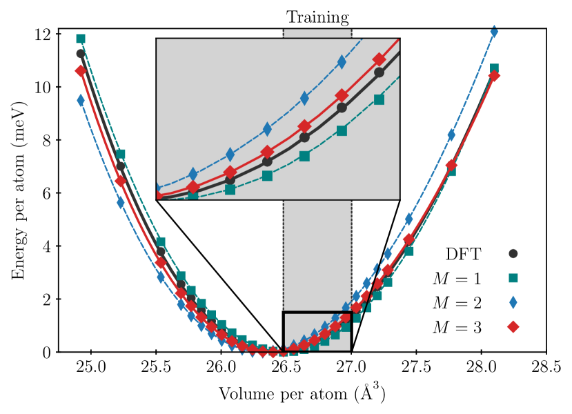
Figure 1: EOS (energy vs. volume) computed with PBEsol-DFT (black dots) compared to so3krates with different numbers of interaction steps $M$. The connecting lines have been obtained by fitting the Vinet EOS. Inset: Zoom into the region of volumes that were covered during the training indicated by the gray shading.

so3krates with three interaction steps ($M{=}3$) yields the best visual agreement for the energy-volume curve in Fig. 1, and the best equilibrium volume. To quantify the agreement, we evaluate the Vinet EOS and extract the cohesive properties equilibrium volume $V_{0}$, isothermal Bulk modulus $B_{0}$, and its pressure derivative $B_{0}^{\prime}$ (functional forms are given in the Supp. Mat.). Results are listed in Table 5.

	DFT	$M{=}1$	$M{=}2$	$M{=}3$
$B_{0}$ ($\mathrm{e}\mathrm{V}\mathrm{/}\mathrm{\text{\AA}}^{3}$)	$0.230$	$0.236$	$0.229$	$0.223$
$B_{p}$ ($\mathrm{e}\mathrm{V}\mathrm{/}\mathrm{\text{\AA}}^{6}$)	$5.576$	$2.830$	$4.815$	$7.118$
$V_{0}$ ($\mathrm{\text{\AA}}^{3}$)	$26.429$	$26.489$	$26.322$	$26.388$
Error $B_{0}$ ($\mathrm{\char 37\relax}$)	–	$2.58$	$-0.47$	$-3.14$
Error $B_{p}$ ($\mathrm{\char 37\relax}$)	–	$-49.25$	$-13.64$	$27.66$
Error $V_{0}$ ($\mathrm{\char 37\relax}$)	–	$0.22$	$-0.40$	$-0.16$

Table 5: Cohesive properties of SnSe for PBEsol-DFT, and so3krates with different numbers of interaction steps $M$ obtained via the Vinet EOS. Best values are highlighted. Values are in good agreement with existing literature Lamuta et al. (2018).

For so3krates with three interaction steps ($M{=}3$), the predicted volume deviates by $-0.16\text{\,}\mathrm{\char 37\relax}$ from the DFT reference, and the deviation of the bulk modulus is $-3.14\text{\,}\mathrm{\char 37\relax}$. A larger error is seen for the pressure derivative of the bulk modulus, $B_{0}^{\prime}$, which deviates by $27.7\text{\,}\mathrm{\char 37\relax}$, indicating worse agreement further away from the training region. Overall, the agreement between DFT and so3krates when predicting cohesive properties can be considered satisfactory. The energy-volume predictions are very good, and transfer even to volumes that are larger or smaller then the ones seen during training.

Finally we check the internal consistency of energy and stress predictions with so3krates by fitting energy-volume and pressure-volume curves and verify that they yield identical parameters for the EOS. Results are shown in Fig. 2. As seen there, results are in perfect agreement, which verifies that stress and resulting pressure are consistent with the underlying energy function as expressed in Eq. 8.

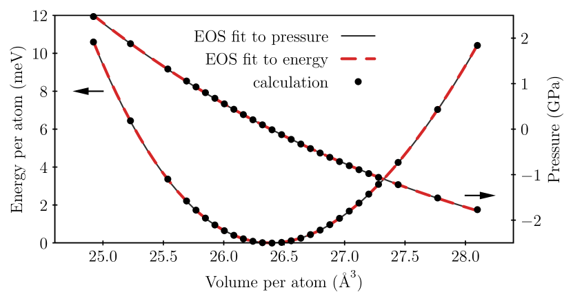
Figure 2: Comparison of EOS obtained by fitting energy-volume (red dashed) and pressure-volume (black solid) data. The results are in perfect agreement.

Source	Method	$\kappa$ (W/mK)	$\kappa_{\text{x}}$	$\kappa_{\text{y}}$	$\kappa_{\text{z}}$
This work	so3krates, $M{=}1$	$0.99\pm 0.10$	$0.53\pm 0.03$	$1.31\pm 0.13$	$1.12\pm 0.12$
"	so3krates, $M{=}2$	$1.13\pm 0.07$	$0.48\pm 0.04$	$1.59\pm 0.07$	$1.20\pm 0.07$
"	so3krates, $M{=}3$	$1.13\pm 0.10$	$0.56\pm 0.05$	$1.56\pm 0.15$	$1.32\pm 0.16$
Brorsson et al. Brorsson et al. (2021)	FCP	$1.12$	$0.57$	$1.46$	$1.32$
Liu et al. Liu et al. (2021)	MLP	$0.86\pm 0.13$	$0.57\pm 0.05$	$1.25\pm 0.24$	$0.76\pm 0.08$
Knoop et al. Knoop et al. (2022)	DFT (extrapolated)	$1.40\pm 0.39$	–	–	–
Review by Wei et al. Wei et al. (2016)	Experiments	$0.45$ to $1.9$	–	–	–

Table 6: Thermal conductivity $\kappa$ of tin selenide at $300\text{\,}\mathrm{K}$.

VI.0.3 Thermal Conductivity

Finally, we proceed to GK calculations, following the approach outlined in our previous workKnoop, Carbogno, and Scheffler (2022); Langer et al. (2023). Finding that simulation cells with $N{=}$864$$ atoms and a simulation duration of $t_{0}{=}$1\text{\,}\mathrm{n}\mathrm{s}$$ yield converged results (see Supp. Mat.), we run $11$ MD simulations using the glp package and so3krates, computing $\bm{J}$ at every step.

Table 6 shows the result: For $M{=}2,3$, so3krates in excellent agreement with the work by Brorsson et al. Brorsson et al. (2021), which uses a force constant potential (FCP). A larger difference is observed with the work by Liu et al. Liu et al. (2021), who, however, use the PBE exchange-correlation functional, as opposed to PBEsol, which was used for the present work. The observed thermal conductivity is consistent with experiments, as well as the size-extrapolated DFT result of Knoop et al. Knoop et al. (2022). The anisotropy of $\bm{\kappa}$ in SnSe is captured as well. Overall, so3krates with more than one interaction step is able to capture the converged thermal conductivity of SnSe, using only training data from the thermalization step of a full aiGK workflow; long-running equilibrium ab initio MD simulations, the bottleneck of the GK method, have been avoided.

VII Conclusion

We demonstrated that the stress and heat flux can be computed efficiently with AD for potentials based on a graph of atom-pair vectors, which we termed GLPs, and provided example implementations in the glp package Langer (2023). Numerical experiments for Lennard-Jones argon and tin selenide with the so3krates GLP, verified that these quantities are computed correctly and consistently. The equivariant so3krates GLP was shown to predict cohesive properties and thermal conductivity of SnSe in good agreement with DFT, other MLPs, and experiments, confirming the practical relevance of computational access to stress and heat flux.

This work enables the use of a large class of recently developed MLPs, those which can be described in the GLP framework, in computational materials science, and in particular for the calculation of thermal conductivities using the GK method. For GLPs implemented with jax, the glp package is provided to enable the calculation of stress and heat flux without requiring further implementation efforts.

Data and Code Availability

The data and code that support the findings of this study are available at doi:10.5281/zenodo.7852530 and at https://github.com/sirmarcel/glp-archive. The glp package is available at https://github.com/sirmarcel/glp. The so3krates model is implemented in mlff, available at https://github.com/thorben-frank/mlff. Further information can be found in the Supp. Mat. and at https://marcel.science/glp.

Author Declarations

Conflict of Interest

The authors have no conflicts to disclose.

Author Contributions

Marcel F. Langer: Conceptualization; Writing – original draft (lead); Writing – review & editing (lead); Software (lead); Visualization (equal); Investigation (equal); Project administration. J. Thorben Frank: Writing – original draft (supporting); Writing – review & editing (supporting); Software (supporting); Investigation (equal). Florian Knoop: Writing – original draft (supporting); Writing – review & editing (supporting); Visualization (equal); Investigation (equal).

References

- Tuckerman (2010) M. E. Tuckerman, Statistical Mechanics: Theory and Molecular Simulation (Oxford University Press, 2010).
- Car and Parrinello (1985) R. Car and M. Parrinello, “Unified approach for molecular dynamics and density-functional theory,” Phys. Rev. Lett. 55, 2471–2474 (1985).
- Teale et al. (2022) A. M. Teale, T. Helgaker, A. Savin, C. Adamo, B. Aradi, A. V. Arbuznikov, P. W. Ayers, E. J. Baerends, V. Barone, P. Calaminici, E. Cancès, E. A. Carter, P. K. Chattaraj, H. Chermette, I. Ciofini, T. D. Crawford, F. De Proft, J. F. Dobson, C. Draxl, T. Frauenheim, E. Fromager, P. Fuentealba, L. Gagliardi, G. Galli, J. Gao, P. Geerlings, N. Gidopoulos, P. M. W. Gill, P. Gori-Giorgi, A. Görling, T. Gould, S. Grimme, O. Gritsenko, H. J. A. Jensen, E. R. Johnson, R. O. Jones, M. Kaupp, A. M. Köster, L. Kronik, A. I. Krylov, S. Kvaal, A. Laestadius, M. Levy, M. Lewin, S. Liu, P.-F. Loos, N. T. Maitra, F. Neese, J. P. Perdew, K. Pernal, P. Pernot, P. Piecuch, E. Rebolini, L. Reining, P. Romaniello, A. Ruzsinszky, D. R. Salahub, M. Scheffler, P. Schwerdtfeger, V. N. Staroverov, J. Sun, E. Tellgren, D. J. Tozer, S. B. Trickey, C. A. Ullrich, A. Vela, G. Vignale, T. A. Wesolowski, X. Xu, and W. Yang, “Dft exchange: sharing perspectives on the workhorse of quantum chemistry and materials science,” Phys. Chem. Chem. Phys. 24, 28700–28781 (2022).
- González (2011) M. González, “Force fields and molecular dynamics simulations,” J. Neutron. 12, 169–200 (2011).
- Lorenz, Groß, and Scheffler (2004) S. Lorenz, A. Groß, and M. Scheffler, “Representing high-dimensional potential-energy surfaces for reactions at surfaces by neural networks,” Chem. Phys. Lett. 395, 210–215 (2004).
- Li et al. (2006) G. Li, J. Hu, S.-W. Wang, P. G. Georgopoulos, J. Schoendorf, and H. Rabitz, “Random sampling-high dimensional model representation (RS-HDMR) and orthogonality of its different order component functions,” J. Phys. Chem. A 110, 2474–2485 (2006).
- Behler and Parrinello (2007) J. Behler and M. Parrinello, “Generalized neural-network representation of high-dimensional potential-energy surfaces,” Phys. Rev. Lett. 98, 146401 (2007).
- Bartók et al. (2010) A. P. Bartók, M. C. Payne, R. Kondor, and G. Csányi, “Gaussian approximation potentials: The accuracy of quantum mechanics, without the electrons,” Phys. Rev. Lett. 104, 136403 (2010).
- Chmiela et al. (2018) S. Chmiela, H. E. Sauceda, K.-R. Müller, and A. Tkatchenko, “Towards exact molecular dynamics simulations with machine-learned force fields,” Nat. Commun. 9, 3887 (2018).
- Chmiela et al. (2019) S. Chmiela, H. E. Sauceda, I. Poltavsky, K.-R. Müller, and A. Tkatchenko, “sGDML: Constructing accurate and data efficient molecular force fields using machine learning,” Comput. Phys. Comm. 240, 38–45 (2019).
- Poltavsky and Tkatchenko (2021) I. Poltavsky and A. Tkatchenko, “Machine learning force fields: Recent advances and remaining challenges,” J. Phys. Chem. Lett. 12, 6551–6564 (2021).
- Noé et al. (2020) F. Noé, A. Tkatchenko, K.-R. Müller, and C. Clementi, “Machine learning for molecular simulation,” Annu. Rev. Phys. Chem. 71, 361–390 (2020).
- Unke et al. (2020) O. T. Unke, D. Koner, S. Patra, S. Käser, and M. Meuwly, “High-dimensional potential energy surfaces for molecular simulations: From empiricism to machine learning,” Mach. Learn. Sci. Tech. 1, 013001 (2020).
- Keith et al. (2021) J. A. Keith, V. Vassilev-Galindo, B. Cheng, S. Chmiela, M. Gastegger, K.-R. Müller, and A. Tkatchenko, “Combining machine learning and computational chemistry for predictive insights into chemical systems,” Chem. Rev. 121, 9816–9872 (2021).
- Unke et al. (2021a) O. T. Unke, S. Chmiela, H. E. Sauceda, M. Gastegger, I. Poltavsky, K. T. Schütt, A. Tkatchenko, and K.-R. Müller, “Machine learning force fields,” Chem. Rev. 121, 10142–10186 (2021a).
- Unke et al. (2022) O. T. Unke, M. Stöhr, S. Ganscha, T. Unterthiner, H. Maennel, S. Kashubin, D. Ahlin, M. Gastegger, L. Medrano Sandonas, A. Tkatchenko, and K.-R. Müller, “Accurate machine learned quantum-mechanical force fields for biomolecular simulations,” (2022), arXiv:2205.08306 .
- Csányi et al. (2004) G. Csányi, T. Albaret, M. C. Payne, and A. De Vita, ““learn on the fly”: A hybrid classical and quantum-mechanical molecular dynamics simulation,” Phys. Rev. Lett. 93, 175503 (2004).
- Jinnouchi et al. (2020) R. Jinnouchi, K. Miwa, F. Karsai, G. Kresse, and R. Asahi, “On-the-fly active learning of interatomic potentials for large-scale atomistic simulations,” J. Phys. Chem. Lett. 11, 6946–6955 (2020).
- Verdi et al. (2021) C. Verdi, F. Karsai, P. Liu, R. Jinnouchi, and G. Kresse, “Thermal transport and phase transitions of zirconia by on-the-fly machine-learned interatomic potentials,” NPJ Comput. Mater. 7, 156 (2021).
- van der Oord et al. (2022) C. van der Oord, M. Sachs, D. P. Kovács, C. Ortner, and G. Csányi, “Hyperactive learning (hal) for data-driven interatomic potentials,” (2022), arXiv:2210.04225 .
- Xie et al. (2022) Y. Xie, J. Vandermause, S. Ramakers, N. H. Protik, A. Johansson, and B. Kozinsky, “Uncertainty-aware molecular dynamics from bayesian active learning: Phase transformations and thermal transport in SiC,” (2022), arXiv:2203.03824 .
- Gilmer et al. (2017) J. Gilmer, S. S. Schoenholz, P. F. Riley, O. Vinyals, and G. E. Dahl, “Neural message passing for quantum chemistry,” in Proceedings of the 34th International Conference on Machine Learning (ICML 2017), Sydney, Australia, August 6–11 (PMLR, 2017) pp. 1263–1272.
- Thomas et al. (2018) N. Thomas, T. Smidt, S. Kearnes, L. Yang, L. Li, K. Kohlhoff, and P. Riley, “Tensor field networks: Rotation- and translation-equivariant neural networks for 3d point clouds,” in NeurIPS 2018 Workshop on Machine Learning for Molecules and Materials, Montréal, Canada, December 8 (Curran Assoc., 2018).
- Drautz (2019) R. Drautz, “Atomic cluster expansion for accurate and transferable interatomic potentials,” Phys. Rev. B 99, 249901 (2019).
- Griewank and Walther (2008) A. Griewank and A. Walther, Evaluating Derivatives (Society for Industrial and Applied Mathematics, 2008).
- Baydin et al. (2017) A. G. Baydin, B. A. Pearlmutter, A. A. Radul, and J. M. Siskind, “Automatic differentiation in machine learning: A survey,” J. Mach. Learn. Res. 18, 5595–5637 (2017).
- Schoenholz and Cubuk (2020) S. Schoenholz and E. D. Cubuk, “Jax md: A framework for differentiable physics,” in Advances in Neural Information Processing Systems 33 (NeurIPS 2020), virtual, December 6–12 (Curran Assoc., 2020) pp. 11428–11441, not available .
- Schütt et al. (2018a) K. T. Schütt, P. Kessel, M. Gastegger, K. A. Nicoli, A. Tkatchenko, and K.-R. Müller, “SchNetPack: A deep learning toolbox for atomistic systems,” J. Chem. Theor. Comput. 15, 448–455 (2018a).
- Unke and Meuwly (2019) O. T. Unke and M. Meuwly, “PhysNet: A neural network for predicting energies, forces, dipole moments, and partial charges,” J. Chem. Theor. Comput. 15, 3678–3693 (2019).
- Schütt et al. (2023) K. T. Schütt, S. S. P. Hessmann, N. W. A. Gebauer, J. Lederer, and M. Gastegger, “Schnetpack 2.0: A neural network toolbox for atomistic machine learning,” J. Chem. Phys. 158, 144801 (2023).
- Louwerse and Baerends (2006) M. J. Louwerse and E. J. Baerends, “Calculation of pressure in case of periodic boundary conditions,” Chem. Phys. Lett. 421, 138–141 (2006).
- Torii, Nakano, and Ohara (2008) D. Torii, T. Nakano, and T. Ohara, “Contribution of inter- and intramolecular energy transfers to heat conduction in liquids,” J. Chem. Phys. 128, 044504 (2008).
- Thompson, Plimpton, and Mattson (2009) A. P. Thompson, S. J. Plimpton, and W. Mattson, “General formulation of pressure and stress tensor for arbitrary many-body interaction potentials under periodic boundary conditions,” J. Chem. Phys. 131, 154107 (2009).
- Volz and Chen (1999) S. G. Volz and G. Chen, “Molecular dynamics simulation of thermal conductivity of silicon nanowires,” Appl. Phys. Lett. 75, 2056–2058 (1999).
- Chen (2006) Y. Chen, “Local stress and heat flux in atomistic systems involving three-body forces,” J. Chem. Phys. 124, 054113 (2006).
- Guajardo-Cuéllar, Go, and Sen (2010) A. Guajardo-Cuéllar, D. B. Go, and M. Sen, “Evaluation of heat current formulations for equilibrium molecular dynamics calculations of thermal conductivity,” J. Chem. Phys. 132, 104111 (2010).
- Fan et al. (2015) Z. Fan, L. F. C. Pereira, H.-Q. Wang, J.-C. Zheng, D. Donadio, and A. Harju, “Force and heat current formulas for many-body potentials in molecular dynamics simulations with applications to thermal conductivity calculations,” Phys. Rev. B 92, 094301 (2015).
- Marcolongo, Umari, and Baroni (2015) A. Marcolongo, P. Umari, and S. Baroni, “Microscopic theory and quantum simulation of atomic heat transport,” Nat. Phys. 12, 80–84 (2015).
- Carbogno, Ramprasad, and Scheffler (2017) C. Carbogno, R. Ramprasad, and M. Scheffler, “Ab initio Green-Kubo approach for the thermal conductivity of solids,” Phys. Rev. Lett. 118, 175901 (2017).
- Boone, Babaei, and Wilmer (2019) P. Boone, H. Babaei, and C. E. Wilmer, “Heat flux for many-body interactions: Corrections to LAMMPS,” J. Chem. Theor. Comput. 15, 5579–5587 (2019).
- Surblys et al. (2019) D. Surblys, H. Matsubara, G. Kikugawa, and T. Ohara, “Application of atomic stress to compute heat flux via molecular dynamics for systems with many-body interactions,” Phys. Rev. E 99, 051301 (2019).
- Langer et al. (2023) M. F. Langer, F. Knoop, C. Carbogno, M. Scheffler, and M. Rupp, “Heat flux for semi-local machine-learning potentials,” (2023), arXiv:2303.14434 .
- Bradbury et al. (2018) J. Bradbury, R. Frostig, P. Hawkins, M. J. Johnson, C. Leary, D. Maclaurin, G. Necula, A. Paszke, J. VanderPlas, S. Wanderman-Milne, and Q. Zhang, “JAX: composable transformations of Python+NumPy programs,” (2018).
- Langer (2023) M. F. Langer, “glp: tools for graph machine learning potentials,” (2023).
- Lennard-Jones (1924) J. E. Lennard-Jones, “On the determination of molecular fields: I. from the variation of the viscosity of a gas with temperature,” Proceedings of the Royal Society of London. Series A, Containing Papers of a Mathematical and Physical Character 106, 441–462 (1924).
- Frank, Unke, and Müller (2022) T. Frank, O. Unke, and K.-R. Müller, “So3krates: Equivariant attention for interactions on arbitrary length-scales in molecular systems,” in Advances in Neural Information Processing Systems 35 (NeurIPS 2022), New Orleans, Louisiana, USA, Nov 28–Dec 9 (Curran Assoc., 2022) pp. 29400–29413.
- Rumelhart, Hinton, and Williams (1986) D. E. Rumelhart, G. E. Hinton, and R. J. Williams, “Learning representations by back-propagating errors,” Nature 323, 533–536 (1986).
- Schmitz, Müller, and Chmiela (2022) N. F. Schmitz, K.-R. Müller, and S. Chmiela, “Algorithmic differentiation for automated modeling of machine learned force fields,” J. Phys. Chem. Lett. 13, 10183–10189 (2022).
- Note (1) Non-periodic systems can be formally accommodated by setting such that replicas lie outside the interaction cutoff radius. The glp framework supports non-periodic systems.
- Langer, Goeßmann, and Rupp (2022) M. F. Langer, A. Goeßmann, and M. Rupp, “Representations of molecules and materials for interpolation of quantum-mechanical simulations via machine learning,” NPJ Comput. Mater. 8, 41 (2022).
- Schütt et al. (2017) K. T. Schütt, P.-J. Kindermans, H. E. Sauceda, S. Chmiela, A. Tkatchenko, and K.-R. Müller, “SchNet: A continuous-filter convolutional neural network for modeling quantum interactions,” in Advances in Neural Information Processing Systems 30 (NIPS 2017), Los Angeles, California, December 4–9 (Curran Assoc., 2017).
- Schütt et al. (2018b) K. T. Schütt, H. E. Sauceda, P.-J. Kindermans, A. Tkatchenko, and K.-R. Müller, “SchNet—a deep learning architecture for molecules and materials,” J. Chem. Phys. 148, 241722 (2018b).
- Klicpera, Groß, and Günnemann (2020) J. Klicpera, J. Groß, and S. Günnemann, “Directional message passing for molecular graphs,” in Proceedings of the Eighth International Conference on Learning Representations (ICLR 2020), Addis Ababa, Ethiopia, April 26–May 1 (OpenReview, 2020).
- Batzner et al. (2022) S. Batzner, A. Musaelian, L. Sun, M. Geiger, J. P. Mailoa, M. Kornbluth, N. Molinari, T. E. Smidt, and B. Kozinsky, “E(3)-equivariant graph neural networks for data-efficient and accurate interatomic potentials,” Nat. Commun. 13, 1–11 (2022).
- Unke et al. (2021b) O. T. Unke, S. Chmiela, M. Gastegger, K. T. Schütt, H. E. Sauceda, and K.-R. Müller, “SpookyNet: Learning force fields with electronic degrees of freedom and nonlocal effects,” Nat. Commun. 12, 7273 (2021b).
- Batatia et al. (2022a) I. Batatia, D. P. Kovács, G. N. C. Simm, C. Ortner, and G. Csányi, “Mace: Higher order equivariant message passing neural networks for fast and accurate force fields,” in Advances in Neural Information Processing Systems 35 (NeurIPS 2022), New Orleans, Louisiana, USA, Nov 28–Dec 9 (Curran Assoc., 2022) pp. 11423–11436.
- Batatia et al. (2022b) I. Batatia, S. Batzner, D. P. Kovács, A. Musaelian, G. N. C. Simm, R. Drautz, C. Ortner, B. Kozinsky, and G. Csányi, “The design space of E(3)-equivariant atom-centered interatomic potentials,” (2022b), arXiv:2205.06643 .
- Bochkarev et al. (2022) A. Bochkarev, Y. Lysogorskiy, C. Ortner, G. Csányi, and R. Drautz, “Multilayer atomic cluster expansion for semilocal interactions,” Phys. Rev. Res. 4, L042019 (2022).
- Knuth et al. (2015) F. Knuth, C. Carbogno, V. Atalla, V. Blum, and M. Scheffler, “All-electron formalism for total energy strain derivatives and stress tensor components for numeric atom-centered orbitals,” Comput. Phys. Comm. 190, 33–50 (2015).
- Admal and Tadmor (2011) N. C. Admal and E. B. Tadmor, “Stress and heat flux for arbitrary multibody potentials: A unified framework,” J. Chem. Phys. 134, 184106 (2011).
- Schütt et al. (2018c) K. T. Schütt, P. Kessel, M. Gastegger, K. Nicoli, A. Tkatchenko, and K.-R. Müller, “SchNetPack: A deep learning toolbox for atomistic systems,” (2018c), arXiv:1809.01072 .
- (62) The schnetpack software library is publicly available at https://github.com/atomistic-machine-learning/schnetpack/ under the MIT license.
- (63) The nequip software library is publicly available at https://github.com/mir-group/nequip under the MIT license.
- Note (2) For instance, Eq. 10 and Eq. 13 yield incorrect results if the MIC is implemented using fractional coordinates, rather than the definition using offsets.
- Green (1952) M. S. Green, “Markoff random processes and the statistical mechanics of time-dependent phenomena,” J. Chem. Phys. 20, 1281–1295 (1952).
- Kubo (1957) R. Kubo, “Statistical-mechanical theory of irreversible processes. i. general theory and simple applications to magnetic and conduction problems,” J. Phys. Soc. Jpn. 12, 570–586 (1957).
- Kubo, Yokota, and Nakajima (1957) R. Kubo, M. Yokota, and S. Nakajima, “Statistical-mechanical theory of irreversible processes. ii. response to thermal disturbance,” J. Phys. Soc. Jpn. 12, 1203–1211 (1957).
- Hardy (1963) R. J. Hardy, “Energy-flux operator for a lattice,” Phys. Rev. 132, 168 (1963).
- Larsen et al. (2017) A. H. Larsen, J. J. Mortensen, J. Blomqvist, I. E. Castelli, R. Christensen, M. Dułak, J. Friis, M. N. Groves, B. Hammer, C. Hargus, E. D. Hermes, P. C. Jennings, P. B. Jensen, J. Kermode, J. R. Kitchin, E. L. Kolsbjerg, J. Kubal, K. Kaasbjerg, S. Lysgaard, J. B. Maronsson, T. Maxson, T. Olsen, L. Pastewka, A. Peterson, C. Rostgaard, J. Schiøtz, O. Schütt, M. Strange, K. S. Thygesen, T. Vegge, L. Vilhelmsen, M. Walter, Z. Zeng, and K. W. Jacobsen, “The atomic simulation environment—a python library for working with atoms,” J. Phys. Condens. Matter 29, 273002 (2017).
- McGaughey and Kaviany (2004) A. J. McGaughey and M. Kaviany, “Thermal conductivity decomposition and analysis using molecular dynamics simulations. part i. lennard-jones argon,” Int. J. Heat Mass Trans. 47, 1783–1798 (2004).
- Knoop et al. (2022) F. Knoop, T. A. R. Purcell, M. Scheffler, and C. Carbogno, “Anharmonicity in thermal insulators – an analysis from first principles,” (2022), arXiv:2209.12720 .
- (72) “Dataset aiGK_for_anharmonic_solids on the NOMAD repository available at doi:10.17172/nomad/2021.11.11-1,” .
- Vinet et al. (1987) P. Vinet, J. Ferrante, J. H. Rose, and J. R. Smith, “Compressibility of solids,” J. Geophys. Res. 92, 9319 (1987).
- Hebbache and Zemzemi (2004) M. Hebbache and M. Zemzemi, “Ab initio study of high-pressure behavior of a low compressibility metal and a hard material: Osmium and diamond,” Phys. Rev. B 70, 224107 (2004).
- Blum et al. (2009) V. Blum, R. Gehrke, F. Hanke, P. Havu, V. Havu, X. Ren, K. Reuter, and M. Scheffler, “Ab initio molecular simulations with numeric atom-centered orbitals,” Comput. Phys. Comm. 180, 2175–2196 (2009).
- Perdew et al. (2008) J. P. Perdew, A. Ruzsinszky, G. I. Csonka, O. A. Vydrov, G. E. Scuseria, L. A. Constantin, X. Zhou, and K. Burke, “Restoring the Density-Gradient Expansion for Exchange in Solids and Surfaces,” Phys. Rev. Lett. 100, 136406 (2008).
- Lamuta et al. (2018) C. Lamuta, D. Campi, L. Pagnotta, A. Dasadia, A. Cupolillo, and A. Politano, “Determination of the mechanical properties of SnSe, a novel layered semiconductor,” J Phys Chem Solids 116, 306–312 (2018).
- Brorsson et al. (2021) J. Brorsson, A. Hashemi, Z. Fan, E. Fransson, F. Eriksson, T. Ala-Nissila, A. V. Krasheninnikov, H.-P. Komsa, and P. Erhart, “Efficient calculation of the lattice thermal conductivity by atomistic simulations with ab initio accuracy,” Adv. Theor. Simulat. 5, 2100217 (2021).
- Liu et al. (2021) H. Liu, X. Qian, H. Bao, C. Zhao, and X. Gu, “High-temperature phonon transport properties of SnSe from machine-learning interatomic potential,” J. Phys. Condens. Matter 33, 405401 (2021).
- Wei et al. (2016) P.-C. Wei, S. Bhattacharya, J. He, S. Neeleshwar, R. Podila, Y. Y. Chen, and A. M. Rao, “The intrinsic thermal conductivity of SnSe,” Nature 539, E1–E2 (2016).
- Knoop, Carbogno, and Scheffler (2022) F. Knoop, C. Carbogno, and M. Scheffler, “Ab initio Green-Kubo simulations of thermal transport in solids: Method and implementation,” (2022), arXiv:2209.01139 .