Get Back Here: Robust Imitation by Return-to-Distribution Planning

Abstract

We consider the Imitation Learning (IL) setup where expert data are not collected on the actual deployment environment but on a different version. To address the resulting distribution shift, we combine behavior cloning (BC) with a planner that is tasked to bring the agent back to states visited by the expert whenever the agent deviates from the demonstration distribution. The resulting algorithm, POIR, can be trained offline, and leverages online interactions to efficiently fine-tune its planner to improve performance over time. We test POIR on a variety of human-generated manipulation demonstrations in a realistic robotic manipulation simulator and show robustness of the learned policy to different initial state distributions and noisy dynamics.

Keywords: Imitation Learning, Behavior Cloning, Model Predictive Control

1 Introduction

Imitation Learning (IL) is a paradigm in sequential decision making where an agent uses offline expert trajectories to mimic the expert’s behavior [1]. While Reinforcement Learning (RL) requires an additional reward signal that can be hard to specify in practice, IL only requires expert trajectories that can be easier to collect. In part due to its simplicity, IL has been applied successfully in several real world tasks, from robotic manipulation [2, 3, 4] to autonomous driving [5, 6].
A key challenge in deploying IL, however, is that the agent may encounter states in the final deployment environment that were not labeled by the expert offline [7]. In applications such as healthcare [8, 9] and robotics [10, 11], online experimentation can be risky (e.g., on human patients) or costly to label (e.g., off-policy robotic datasets can take months to collect). In this work, we are thus interested in methods that are both robust in states not seen during training and also able to adapt online without access to a queryable expert.
Typical Imitation Learning approaches such as Behavior Cloning (BC) [1] and Adversarial Imitation Learning (AIL) [12] are not designed to be both data efficient and robust to distribution mismatch between the expert data and the final deployment environment. BC treats IL as a supervised learning problem, maximizing the likelihood of taking an expert action under the state distribution of the expert [1]. While BC generates useful policies from offline expert data, it performs poorly in states not seen during training [7]: not only is BC brittle to out-of-distribution (OOD) inputs, it does not have access to a queryable expert and thus cannot adapt to new states once deployed. In contrast, AIL methods use an Inverse Reinforcement Learning (IRL) approach, first learning a reward function under which the expert trajectory data is optimal, and then training a policy using this learned reward function [13, 12, 14]. Since AIL methods train a Reinforcement Learning policy directly in the deployed environment, they can learn a policy in states not initially seen in the expert data. Nevertheless, AIL methods require large amounts of online data to reach expert performance and are typically hard to tune in practice [15], while BC uses no online data and is simpler to tune.
This paper proposes to take advantage of BC’s data-efficiency and ability to train offline, while leveraging the flexibility of offline model-based methods [16, 17, 18] to be robust to out-of-distribution states and to fine-tune the final policy once deployed. POIR (Planning from Offline Imitation Rewards), a Model-Based Imitation Learning algorithm, can learn a robust policy using an offline dataset of expert demonstrations (i.e. without any rewards), and continue to improve from data collected in the environment once deployed. Through the use of an explicit imitation reward used during planning, POIR can return to states that were seen in the expert data if it ends up is states that are outside of the expert’s support.
POIR can be deployed in both the offline and online settings. In the offline setting, the BC policy and the world model used by the planner are trained only on offline expert transitions. In the online setting, the world model is fine-tuned on new transitions collected by the planner policy in the deployed environment, improving the world model’s prediction accuracy on parts of the state space not covered by offline transitions; this in turn improves the planner policy performance in out-of-distribution states with respect to the offline expert data.
Our contributions in this work are twofold: First, we introduce POIR, a Model-Based Imitation Learning method that is robust to both initial state distribution perturbations and stochasticity in the deployed environment. We demonstrate its performance compared to BC and AIL methods on a series of complex human-generated robotic manipulation demonstrations on the realistic robosuite [19] simulator. Second, we show that POIR can be trained offline and deployed similarly to BC, while also continuing to improve its performance once online with significantly less data compared to AIL methods, avoiding the complexities of an RL training algorithm and adversarial loss.

2 Method

We model environments as episodic Markov Decision Processes (MDPs) $(S,A,P,r,\rho_{0},T)$ [20], where $S$ denotes the state space, $A$ the action space, $P$ the transition kernel, $r$ the reward function, $\rho_{0}$ the initial state distribution, and $T$ the task horizon. A policy $\pi$ is a mapping from states to a distribution over actions; we denote the space of all policies as $\Pi$. Let $\rho_{\pi}$ denote the distribution over states and actions induced by policy $\pi$. In Imitation Learning, we do not know the true reward $r$. Instead we construct an imitation reward $r_{IL}$ offline based on the expert demonstrations $D_{e}=\{(s_{t},a_{t},s_{t+1})_{t\in T}\}$ induced by an expert policy $\pi_{e}$.

The goal of Imitation Learning is to find a policy $\pi$ such that its induced state-action distribution $\rho_{\pi}$ minimizes some divergence $D$ to the state-action distribution of the expert $\rho_{\pi_{E}}$ [21]. In other words, the goal is to minimize: $\min_{\pi}D(\rho_{\pi},\rho_{\pi_{E}})$. For example, the objective of GAIL [12] is to minimize a regularized form of the Jensen-Shannon divergence.

Next, we present POIR: a Model-based Imitation Learning algorithm that leverages an offline dataset of human expert demonstrations for robust imitation learning, while further improving with online data collected in the environment. POIR is composed of three main components: the BC policy prior, the planner, and the imitation reward.

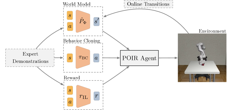
Figure 1: Overview of various POIR components and their dependencies. The BC policy and world model are trained from the expert data, whereas the imitation reward can depend either on the expert data, the world model’s ensemble discrepancy, or the BC policy’s ensemble discrepancy.

2.1 General Approach

Our general approach extends the existing advantages inherent in BC with the ability of a planning algorithm to produce robust actions and adapt efficiently online. We do this by using the BC policy as a prior to guide trajectory rollouts in the planner. The planner uses a learnt world model to generate trajectories, and then selects the best action ranked according to a reward function; we leverage an imitation reward to incentivize the agent to stay close to the expert’s support. All components of the system are initially trained on the dataset of expert trajectories $D_{e}=\{(s_{t},a_{t},s_{t+1})_{t\in T}\}$. Details about the three core components of POIR (the BC prior policy, the planner, and the imitation reward) are provided in the following sections and illustrated in Figure 1. An overview of POIR can be found in Algorithm 1.

2.2 BC Policy Prior

POIR is a planning-based method that leverages BC as a prior to guide planner rollouts. One key aspect of our work is that both the BC policy prior and the world model (Sec. 2.3) are implemented as bootstrap ensembles [22, 23, 24]. Our BC policy prior is in effect an ensemble of $K$ networks, which is used in a round-robin fashion in the planner as described in Sec. 2.3. When using BC as a baseline, however, we have chosen to average the output of the $K$ networks to produce the final output action, which we refer to as Ensemble BC (EBC). This gives our Ensemble BC policy the following form: $\pi_{BC}=\frac{1}{K}\sum_{1}^{K}\pi_{\theta_{k}}(s)$, which shows significant performance gains over single-network BC (see Figure 3), also observed in prior work [25]. We train EBC on the full set of expert demonstrations for a given task, minimizing the action prediction error: $\theta_{k}=\operatorname*{argmin}_{\theta_{k}}\mathbb{E}_{D_{e}}[(\pi_{\theta_{k}}(s_{t})-a_{t})^{2}].$

2.3 Planner

The core of our algorithmic approach is to leverage a planner to return to the expert’s state distribution. POIR uses Model-Predictive Control (MPC) [26] with an MPPI-based [27] trajectory optimizer, modified to support ensembles and policy priors as detailed by [16]. Intuitively, when the policy is already in-distribution relative to the expert demonstrations, the planner does not provide much added value. However when the policy is either strongly out of distribution, or decides to take actions that would result in leaving the distribution, the planner will provide candidate action trajectories that are closer to the demonstration distribution. We provide more details on the learnt world model and the trajectory optimizer below.

World Model A core component of planning-based approaches is the underlying world model. We use a deterministic function $\hat{P}_{\phi}:S\times A\rightarrow S$ parameterized by $\phi$, that takes a state-action pair and outputs the next state. It is learnt on the expert demonstration dataset $D_{e}$: $\operatorname*{argmin}_{\phi}\mathbb{E}_{(s_{t},a_{t},s_{t+1})\in D_{e}}[(\hat{P}_{\phi}(s_{t},a_{t})-s_{t+1})^{2}]$. As mentioned previously, the world model is a bootstrap ensemble; $K$ world models are learned, where each $\hat{P}_{k}$ is trained on the same dataset but with different weight initializations. In the case of deterministic environments, the choice of a deterministic model vs. a stochastic one has been shown not to impact performance much [28]. Although certain experimental environments are stochastic, the demonstration data however is deterministic, and deterministic models have shown to work well in practice for fine-tuning.

Planner trajectories As described above, our policy leverages Model-Predictive Control (MPC) [26], a simple yet effective control strategy [29, 23]. At each policy step, MPC queries a trajectory optimizer to find an optimal trajectory $A_{H}=\{a_{1},\dots,a_{H}\}$ for the current state $s_{t}$, which maximizes some objective function $r$ according to the dynamics of a world model $\hat{P}$. MPC then applies the first action from the trajectory, $a_{1}$, to the system, and observes the corresponding next state $s_{t+1}$, with which the algorithm repeats. POIR leverages a modified version of MPPI [30, 23, 16] which we now show in detail.
POIR’s trajectory optimization scheme involves generating $N$ parallel trajectories sampled from a proposal distribution generated by $\pi_{BC}$. For each trajectory, an action is sampled and pertubed with gaussian noise, $\sim{a}_{t}=\{\pi_{BC}(s_{t})+\epsilon_{i}\}_{i=1}^{N}$ with $\epsilon_{i}\sim\mathcal{N}(0,\sigma^{2})$. The perturbed action $\tilde{a}_{t}$ is then passed into the world model to create the following $\hat{s}_{t+1}=\hat{P}(\hat{s}_{t},\tilde{a}_{t})$. This procedure is repeated $H$ times to create a full action trajectory $A^{n}_{H}=\{\tilde{a}_{1},\dots,\tilde{a}_{H}\}$, in parallel for the $N$ trajectories. The corresponding cumulative reward is also calculated to produce $R^{n}=\sum_{h=1}^{H}r_{IL}(\hat{s}^{n}_{t},{\color[rgb]{0,0,0}\tilde{a}^{n}_{t}})$ for each of the $N$ trajectories.
The final action returned, as per MPC, is the first action from the trajectory $i_{max}=\operatorname*{argmax}_{n}R^{n}$ with the highest reward: $\pi_{\emph{POIR}}(s_{t})=A_{i_{max}}[0]$. The full algorithm is detailed in Algorithm 2.

Use of Ensembles As mentioned previously, both the policy prior $\pi_{BC}$ and the world model $\hat{P}$ are actually composed of $K$ ensembles. These are exploited by allocating each of the $N$ trajectories to one of the ensemble heads, both for the policy prior as well as the world model. The allocation is constant throughout the rollout, as performed by  [23] and  [16], and allows for greater diversity both in action selection and model predictions. For notational simplicity we don’t describe this explicitly in Algorithm 2, but the full algorithm can be found in the Appendix, Algorithm 3.

2.4 Imitation Reward

The last component of POIR is the imitation reward, $r_{IL}$. We construct several reward functions in the following sections, with the criteria that the reward should be high for states that are close to the expert support and low otherwise. The notion of proximity varies for each of our proposed rewards.

L2 Reward One simple way to construct such a reward function is to compute the L2 distance between the current state and all the states in the demonstration data, and then to take the minimum of these distances. This reward function does not require any pre-training. For a state $s$, we denote the L2 reward as: $r_{L2}(s)=-\min_{s_{e}\in D_{e}}||s-s_{e}||_{2}$.

For large datasets, the L2 reward can become computationally expensive as we compute the distance to all states in the expert data. Approximate lookup approaches can reduce the complexity from $O(n)$ to $O(log(n))$ [31, 32]. The L2 reward, albeit simple, has shown to be effective on robotic arm manipulation tasks in previous works [33] and can be extended to higher dimensional state spaces by learning an embedding [33]. The variant of POIR using this reward function is called POIR-L2.

Ensemble-Disagreement Rewards Another formulation of $r_{IL}$ is to consider the disagreement of the predictions over an ensemble of networks trained on the demonstration data. Two well-known approaches use the disagreement of BC policies, as introduced in DRIL [34], and the disagreement of the world models, as introduced in MoREL [17]. The former version is called POIR-DRIL while the latter is called POIR-MOREL. These approaches, when compared to POIR-L2, scale well with the size of the expert dataset and the state dimension, since they need only one forward pass during inference rather than an exhaustive search over $D_{e}$. The rewards can be expressed as $r_{DRIL}(s)=-\max_{i,j}||\pi_{\theta_{i}}(s)-\pi_{\theta_{j}}(s)||_{2}$ and $r_{MOREL}(s,a)=-\max_{i,j}||\hat{P}_{\phi_{i}}(s,a)-\hat{P}_{\phi_{j}}(s,a)||_{2}$.

Algorithm 1 POIR

1:  Input: $D_{e}$: expert trajectories, $L_{steps}$: # of env. steps, $H$: planning horizon, $N$: number of trajectories, $\sigma$: policy prior noise scale.

2:  $\pi_{BC}$, $\hat{P}$, $r_{IL}$ = Train($D_{e}$)

3:  $D_{a}=\{\}$

4:  for $t=1$ to $L_{steps}$ do

5:     Observe $s_{t}$

6:     $a_{t}$ = SelectAction$(s_{t},\pi_{BC},\hat{P},r_{IL},H,N,\sigma,k)$

7:     $s_{t+1}$ = EnvironmentStep($a_{t}$)

8:     $D_{a}=D_{a}\cup\{(s_{t},a_{t},s_{t+1})\}$

9:     Train $\hat{P}$ on $D_{e}\cup D_{a}$

10:  end for

Algorithm 2 POIR-SelectAction

1:  SelectAction($s,\pi_{BC},\hat{P},r_{IL},H,N,\sigma$):

2:  Set $\mathbf{R}=\vec{0}_{N}$ , $\mathbf{A}=\vec{0}_{N,H}$

3:  for $n=1..N$ do

4:     $s_{1}=s$

5:     for $t=1..H$ do

6:        $\epsilon\sim\mathcal{N}(0,\sigma^{2})$

7:        $\tilde{a}_{t}=\pi_{BC}(s_{t})+\epsilon$

8:        $s_{t+1}=\hat{P}(s_{t},\tilde{a}_{t})$

9:        $\mathbf{A}_{n,t}=\tilde{a}_{t}$

10:        $R_{n}=R_{n}+r_{IL}((s_{t},\tilde{a}_{t},s_{t+1}))$

11:     end for

12:  end for

13:  return  $a_{1}=A_{\operatorname*{argmax}R,1}$

2.5 Online Fine-Tuning

We can perform online fine-tuning of POIR once deployed in an environment. The main goal is to fine-tune $\hat{P}$  with additional data gained from interactions with the system. We can do this by simply augmenting the original dataset $D_{e}$ with data from the agent $D_{a}$ and training $\hat{P}$on $D=D_{e}\cup D_{a}$. In the case where imitation rewards use ensemble discrepancy on $\hat{P}$, we maintain a frozen version of $\hat{P}$ trained only on $D_{e}$ for the calculation of the imitation reward.

3 Experiments

To investigate the benefits of POIR in distribution mismatch settings, we train POIR on a series of human demonstration demonstrations on a realistic robotic manipulation tasks, and evaluate POIR’s performance on various physically perturbed versions of the original environment.

3.1 Environments and Demonstrations

Environments We investigate POIR’s performance on a series of robotic manipulation tasks defined in the Robosuite simulation environment [19]. We use these environments since they combine several key properties: the tasks are complex, a large amount of human generated demonstrations is available, and the environment authors have shown strong correlation between simulator performance and on-robot performance [35]. We focus on three tasks of increasing difficulty using the 7-DoF Panda arm model: Lift: grasp & lift a cube off of the table (10-dim observation space), PickPlaceCan: grasp a can and place it in a bin (14-dim observation space), NutAssemblySquare: grasp a square nut and place it on a rod fixture (14-dim observation space). All three tasks are deterministic and contain two sources of variation by default: the initial position of the robotic arm and the initial position of the object to grasp.

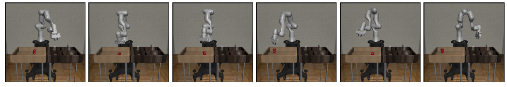
Figure 2: For noise of $\sigma_{noise}=0.4$ shown above, the arm can start in positions much further from the center of the table compared to default noise of $\sigma_{noise}=0.2$. Examples for all environments are shown in Appendix E.

Demonstrations We use open-source human-generated demonstrations from the Robomimic [35] dataset, a well-studied dataset of human-generated demonstrations, for which there is strong evidence that approaches working well in the robosuite simulator also perform well on a real-robot version of the same tasks. For each task, we use the proficient human demonstrations, composed of 200 demonstrations collected from a single proficient human operator using RoboTurk [36].

3.2 Distribution mismatch

The demonstrations are collected in an unperturbed version of the environment, which we refer to as the offline environment. We evaluate the performance of POIR on deployed environments that differ in two different manners: the diversity of the initial state distribution and the stochasticity in the transition dynamics of the environment.

Initial state distribution. For each task (Lift, PickPlaceCan, and NutAssemblySquare), we modify the initial state distribution of the robotic arm in the deployed environment. By default, the initial position of the arm is randomized around a mean position with a Gaussian noise of standard deviation $\sigma_{init}=0.02$. The default noise keeps the arm close to the mean position at the beginning of each episode as depicted in Figure 7. Offline human demonstrations are collected with this default noise. In our experiments, we gradually increase $\sigma_{init}$ in the deployed environment from $0.02$ to $0.4$. For larger $\sigma_{init}$ values, the initial position of the robotic arm can now be at either side of the table rather than centered directly above it, as shown in Figure 2. The overall effect is illustrated in Appendix E and in attached videos. The initial state noise modification leads to a distribution mismatch between the default initial positions in the demonstrations and the ones in the deployed environment.

Stochasticity. We introduce stochasticity to the otherwise deterministic Robosuite environments. Environment stochasticity can emerge in the real-world from naturally occurring variations in the controller or deployed environment e.g., friction, lighting, object deformations. We use a white Gaussian noise with standard deviation $\sigma_{action}$ as a simple model of these external perturbations. The Gaussian noise is added to the action taken by the agent at every step. Therefore the environment becomes stochastic, since two agents that take the same action at the same state may wind up in different next states.

3.3 Implementation details

All algorithms are evaluated on $20$ episodes every $50,000$ environment steps, for a total of $500,000$ steps. Results for each method are averaged over $5$ random seeds. We report the average environment success rate $\in[0,1]$ denoting whether or not the task was successfully completed. For each algorithm, the same set of hyperparameters are used across all environments. A full set of hyperparameters is reported in Appendix C.
Since POIR uses an ensemble of BC policies in the planner, BC and EBC are thus natural baselines. We use the same network architecture (a multi-layer perceptron) for BC, EBC, and the BC policy used in POIR. For POIR and EBC, we use $27$ ensemble networks. For implementation reasons, ensembles are a multiple of 3, and we did not observe performance gains beyond 27. In the planner, we sample $N=4000$ trajectories. We use $\sigma=0.2$ for the standard deviation noise around the BC action proposal. We use $H=5$ as the horizon for the planner trajectories as it performed best during initial hyperparameter searches.
We also compare our algorithm to state of the art imitation learning algorithms: Discriminator Actor-Critic (DAC) [15] tuned using the guidelines of [37], ValueDice [38], and SQIL [14]. DAC, ValueDice, and SQIL are natural baselines for POIR since they leverages both expert demonstrations and online data collected in the environment to learn its final policy. However, DAC and SQIL additionally differ from POIR as they cannot be used fully offline.
We find that state and action normalization helps POIR, but does not provide a benefit to BC or EBC. For DAC, we found that state normalization worked best. We normalize the offline expert demonstrations such that states and actions have mean $0$ and standard deviation $1$. Online transitions are normalized with the offline mean and standard deviation parameters.

3.4 Results: Effects of initial state distribution mismatch

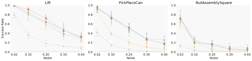
(a) Offline performances

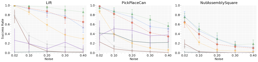
(b) Online performances after 500,000 environment steps

Figure 3: Effects of $\sigma_{init}$ on task success rate for both off-line and on-line scenarios.

Offline Performance. In the fully offline setting, we observe that POIR have the best performances across the environments and noise level. Results for the offline setting are shown in the top row of the Figure 3. For example in PickPlaceCan, Ensemble BC and POIR have nearly the same performance when there is no mismatch, but POIR has a $20\%-30\%$ increase in success rate for $\sigma_{init}=0.1$. This shows that the imitation rewards help the planner find better actions than the prior BC policy proposals in states not seen in the demonstrations.

Online Performance. POIR is able to efficiently leverage online data to improve its performance, as shown in the bottom row of Figure 3. After online fine-tuning with $500,000$ environment steps, POIR-L2 performs best compared to other imitation rewards and BC/IL baselines. For example, there is a 50% gap in success rate between POIR-L2 and EBC for Lift and PickPlaceCan for the largest value of noise ($\sigma_{init}=0.4$). This shows that improving the planner with data collected improves performance. This is a key difference between EBC and POIR as EBC cannot leverage this new data. RL-based approaches (DAC, ValueDICE, and SQIL) perform poorly as soon as some mismatch is introduced except for DAC on PickPlaceCan that achieves 20% of success rate for $\sigma_{init}=0.4$ which is 3 times lower than POIR-L2 which achieve nearly 60% of success rate in that configuration.

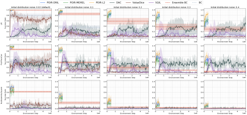
Figure 5: Effects of $\sigma_{init}$ on POIR success rate: POIR is able to maintain better performance compared to BC and DAC baselines across all environments and initial noise values. The performance gap between Ensemble BC and POIR widens as distribution mismatch increases. The shaded areas correspond to one standard deviation around the mean.

Sample efficiency. One of POIR’s main advantages is that offline performance is competitive to BC and EBC baselines and that after an additional $500,000$ fine-tuning steps in the environment, POIR can also reach better performance compared to a state of the art IL method like DAC. In contrast, RL-based approaches (DAC, ValueDICE, and SQIL) are not able to reach BC performance within $500,000$ environment steps for Lift, and has a $0$ success rate even after $5M$ steps for NutAssemblySquare. This is illustrated in the Appendix: Figure 5 shows the training curves for $5M$ environment steps.

Emergent Retrying. Qualitatively, we find that the BC agent moves towards the object of interest, attempts to grab it, and then continues to act as if the object were grasped regardless of whether the grasp was actually successful. On the contrary, we notice in our experiments that POIR is able to retry grasping the object even after failing initial grasp attempts. We show emergent retrying for POIR in the attached video files as well as in the Appendix F.

Real time control. Previous works showed that MPPI based approaches are amenable to real time control [30, 23]. The overhead of POIR on top of MPPI consists in using a BC prior and computing a reward function which are computed with a forward pass on an ensemble of neural networks (and an additional lookup in the case of the L2 reward). We found experimentally that POIR-DRIL and POIR-MoREL run at 10 Hz and that POIR-L2 runs at 5Hz at inference on a TPUv2 GCP machine using a single core of the accelerator, which we argue shows the feasibility of the approach for real-time control.

Ablations. To showcase the importance of each component in POIR, we also ran two other baselines: POIR without a BC prior and PPO [39] with the DRIL reward which is essentially the DRIL algorithm [34] without the auxiliary BC loss. The results are detailed in Appendix B. Both baselines yielded a 0% success rate across all the experiments. These results show both the importance of the BC prior and the planner/IL reward combination.

3.5 Results: Effects of environment stochasticity mismatch

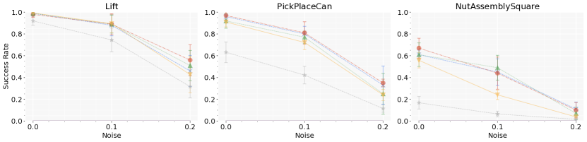
(a) Offline performances

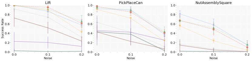
(b) Online performances after 500,000 environment steps

Figure 4: Effects of $\sigma_{action}$ on task success rate for both off-line and on-line scenarios.

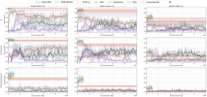
Figure 6: Effects of $\sigma_{action}$ on POIR success rate: This figure describes the effects of action noise on the various evaluated approaches. We can observe that POIR methods are consistently better than other baselines. The shaded areas correspond to one standard deviation around the mean.

As shown in Figure 4, POIR outperforms the other baselines when action noise stochasticity is added. We also remark that online data improves the trained policy. Notably with PickPlaceCan with an action noise of $0.1$, the gap in success rate between Ensemble BC and POIR-L2 is $25\%-35\%$. For NutAssemblySquare, the success rate gap between POIR-L2 and Ensemble BC goes from $0\%$ without action noise to nearly a $15\%$ success rate increase when the action noise is $0.1$. For Lift and NutAssemblySquare, DAC does not learn a good policy within the first $500,000$ environment steps. As shown in the Figure 6, even with $5M$ environment steps, RL-based approaches perform worse than EBC in nearly all settings.

4 Related Work & Limitations

Imitation Learning suffers from distribution shift between the expert data and the policy [1]. [40] formalized this notion and showed that BC has a quadratic regret bound in $T$. Many IL methods have been designed to make policies more robust to distribution shift [7, 41, 13].

IL with Queryable Expert Policy: [7] proposed DAGGER which queries the expert policy on online demonstrations to refine the BC policy and achieve linear regret in $T$. Recent studies use the policy uncertainty to selectively decide when to query the expert [42, 43, 44, 45]. Our IL method does not require a queryable expert or the explicit need for online demonstrations to mitigate distribution shift.

Adversarial Imitation Learning: AIL methods seek to match the state-action distribution of the policy to the fixed expert data by learning a discriminator that differentiates expert from non-expert transitions [12, 15]. A model-free RL policy is trained on online environment trajectories by using the discriminator as a reward. MGAIL [46] uses an additional world model to train a policy on exact gradients of the discriminator over entire trajectories. AIL methods generate a model-free controller that is hard to tune in practice and not sample efficient with respect to online data [12]. We include comparisons to DAC, a state of the art AIL method, in Section 3.4. In contrast to DAC, our method can be deployed offline and is more sample efficient online.

IL with Support: Recent IL methods explicitly use the distribution mismatch between the policy and expert as a reward signal for training a model-free controller, without the need for a discriminator [33, 34, 47, 48, 49]. These methods also require online data collection for training the RL policy, with similar sample efficiency as DAC.

Offline RL: Many offline RL methods use uncertainty estimates to make the final policy robust to distribution shift. Model-based offline RL methods leverage uncertainty in the world model or an ensemble of networks to keep the final policies close to the expert [18, 17, 50, 51, 16, 52]. Offline RL differs from the IL setting as it assumes having access to the environment reward while in IL the environment reward is unknown. Offline RL methods are unadapted to deal with the IL rewards used by POIR. For instance, the L2 reward would be exactly 0 on the dataset of demonstrations.

Model-based Imitation Learning (MBIL): Using world models in Imitation Learning has been explored in other contexts [53, 54]. IMPLANT [55] uses GAIL to learn a policy and value function using online data, which then get used in a planner policy. While IMPLANT shows that their planner is robust in noisy deployed environments for simple locomotion environments (Hopper, HalfCheetah, and Walker2d) our method differs mainly as we use BC instead of GAIL. This difference allows POIR to be deployed offline which is not the case of IMPLANT. Imitative Models [56] learns a density model over expert data and then uses the density model as a reward in a goal conditioned open-loop planner; they demonstrate policies robust to noise in an autonomous driving simulator environment. A follow-up, Robust Imitative Planning (RIP) [57], uses an ensemble of networks to minimize uncertainty of trajectories in the planner, and then adapts the policy online by querying an expert policy [58]. A similar method, RMBIL [59] also shows improvements over BC when deployed in environments that mismatch the expert distribution. RMBIL is a purely offline method, that uses a neural ODE controller with a CVAE to encode states. In contrast to Imitative Models, RIP, RMBIL, and other similar works [60], our method uses a simpler policy: model-predictive control [61] with an open-loop trajectory planning algorithm [16] using BC priors; notably we show that POIR can run in both the offline and online settings without querying an expert.

Generalization in IL/RL: Generalization in IL and RL seeks to improve performance on unseen interactions during deployment [62]. Recent zero-shot and few-shot IL methods are designed to adapt to new tasks, objects, and domains using methods such as goal conditioning [63, 64, 65], meta-learning [66, 67], domain randomization [68, 69, 70]. Generalization improvements have also been shown in RL [71, 72]. Our method explores the setting where the test environment is out-of-distribution compared to expert data, but not on new tasks or objects. We achieve improvements over BC on out-of-distribution test environments through a model-based controller, rather than with goal-conditioning or data augmentation.

Limitations: We foresee three limitations in our approach: As implemented in the paper, the L2 reward used in our experiments does not straightforwardly scale to large datasets, the method may struggle with higher-dimensional state spaces such as images, and experimental results were not validated on a physical robot. In terms of scaling to large datasets, approaches exist to address this limitation such as approximate nearest-neighbour lookups [31, 32]. For handling higher-dimensional observations such as pixels, approaches such as recurrent state-space models [73, 74] or other embeddings [33] where observations are embedded into a latent space could be used to create a more compact representation. Finally, although we did not test our approach on a real robot, evaluation of learning methods on the Robosuite simulator have been shown to correlate well with real-world robot experiments, in particular using the robomimic datasets [35] as we have done in this paper.

5 Conclusion

In summary, we present POIR, an Imitation Learning algorithm that combines BC with a planner. The BC policy creates candidate actions for the planner while the planner selects the best actions that will drive the agent back to states covered by the expert support. Unlike existing approaches, POIR uses a model-based controller that can be deployed either in the offline or online settings, without querying an expert. We demonstrate both the ability to learn entirely off-line, and downstream sample efficiency significantly better than common AIL methods. We demonstrate that POIR generates actions that are significantly more robust to initial state distribution mismatch and stochastic actions in the deployed environment compared to AIL/BC. Finally, we empirically demonstrate that training the world model on online data further improves performance and robustness of the policy to distribution mismatch.

Appendix A Learning Curves

In this section, we show the learning curves until 5M of environment steps.

A.1 Initial State Distribution Mismatch.

A.2 Action Noise.

Appendix B Ablations

We made several ablations in order to reflect the importance of each of the components of the method: the BC prior, the planner, and the IL reward. The ablation experiments of Table-1-2-3 show that each of the components is crucial to the performance of POIR:

• Ensemble BC: this algorithm can be seen as an ablation of our approach as it only relies on the BC prior. The results show that Ensemble BC performs strongly without any distribution mismatch but its performance quickly degrades as the mismatch increases. Therefore, on the expert support, the BC prior selects actions good enough to solve the task but it does not recover from unseen states.

• POIR without a BC prior: in this version, the planner does not rely on BC to pick action candidates and instead samples actions uniformly at random. This leads to 0% success rate across every environments hence showing that the BC prior is crucial.

• PPO + DRIL reward: in this version, we trained the PPO algorithm using the public implementation from acme algorithm to maximize one of the proposed rewards (DRIL). This algorithm yields a 0% success rate across the environments. This shows that the signal from the IL reward alone is not informative enough to solve the task even with an online RL algorithm. However, POIR’s specific combination (BC prior + planner + IL Reward) leverages the reward signal to find the actions that will lead the agent to stay on the expert support where BC is a strong prior.

These ablations show that each component alone is not enough to tackle the distribution mismatch problem: BC cannot recover from unseen states; the planner can only leverage reasonable candidate actions with limited compute; the IL reward alone is too weak of a signal to lead to task completion.

Magnitude	0.02	0.1	0.2	0.3	0.4
POIR-DRIL (online)	1	0.9	0.78	0.65	0.52
POIR-DRIL (offline)	1	0.77	0.65	0.4	0.22
Ensemble BC	1	0.85	0.60	0.38	0.3
PPO-DRIL	0	0	0	0	0
POIR-DRIL (without BC prior)	0	0	0	0	0

Table 1: Ablation of the components of the POIR algorithm on Lift

magnitude	0.02	0.1	0.2	0.3	0.4
POIR-DRIL (online)	0.92	0.83	0.65	0.5	0.4
POIR-DRIL (offline)	0.96	0.75	0.5	0.33	0.25
Ensemble BC	0.87	0.38	0.2	0.1	0.05
PPO-DRIL	0	0	0	0	0
POIR-DRIL (without BC prior)	0	0	0	0	0

Table 2: Ablation of the components of the POIR algorithm on PickPlaceCan.

magnitude	0.02	0.1	0.2	0.3	0.4
POIR-DRIL (online)	0.72	0.38	0.22	0.15	0.08
POIR-DRIL (offline)	0.72	0.33	0.17	0.08	0.03
Ensemble BC	0.62	0.22	0.05	0.03	0.02
PPO-DRIL	0	0	0	0	0
POIR-DRIL (without BC prior)	0	0	0	0	0

Table 3: Ablation of the components of the POIR algorithm on NutAssemblySquare.

Appendix C Hyperparameters & Implementation Details

In this section, we outline the full set of hyperparameters for POIR, BC, and DAC.

C.1 Details for BC, EBC, & POIR.

Offline Training.

For offline training of the BC policy and world models, we use $500$ training epochs, with each epoch doing a full pass on the offline expert trajectories with a batch size of $256$. POIR-DRIL and POIR-MOREL train the imitation reward policy and world models respectively on $50000$ gradient steps on offline data with batch size of $256$. We use an Adam optimizer [75] with a learning rate of 1e-4, $\beta_{1}=0.9$, and $\beta_{2}=0.999$ for all networks.

POIR Online Training.

For POIR online training, we use a replay buffer to store a mixture of expert data and online planner policy data $D=D_{e}\cup D_{a}$. We denote the ratio of online to offline data sampled from the buffer as the $mixture\_ratio$. At the beginning of online fine-tuning, we use a $mixture\_ratio=0.0$, and we linearly increase the ratio to a maximum of $0.5$ by an increment of $0.05$ for every 100 gradient steps. We train online for up to $500k$ environment steps.

Planner

Previous works based on MPPI [30, 23, 16] use a softmax-averaging of the action trajectories according to their respective return, but this can be unstable in the face of large returns. We observe that top-k averaging performs equivalently experimentally while being more numerically stable.

Hyperparameters.

The networks for BC and world models use an MLP with $5$ layers, $relu$ activation functions, and $300$ hidden units. We use a single network for BC and an ensemble of $27$ networks for EBC and world models. We swept over parameters as shown in Table 4, with final values shown in the right-most column. For BC and EBC, we found that normalizing states and actions did not provide a benefit. For POIR, we use both state and action normalization.

Parameter	Sweep	Final Value
Learning rate	{1e-4, 5e-4}	1e-4
Hidden units	{100, 300, 500}	300
Layers	{1, 3, 5}	5
Num Networks	{1, 3, 9, 27}	27
Activation	$\{relu,tanh\}$	$relu$
Planner: Num trajectories $N$	{1000, 4000}	4000
Planner: Action Noise $\sigma$	{0.1, 0.15, 0.2}	0.2
Planner: Horizon $H$	{1, 5, 10, 20}	5
POIR: Normalize observations	{True, False}	True
POIR: Normalize actions	{True, False}	True
BC: Normalize observations	{True, False}	False
BC: Normalize action	{True, False}	False

Table 4: Hyperparameters for EBC, the world model in POIR, and the planner. BC uses the same network hyperparameters, but with a single network only. Both BC and EBC do not make use of the planner.

C.2 Details for the baselines (DAC, ValueDICE, SQIL, PPO+DRIL).

Hyperparameter selection.

For each baseline and hyperparameter set, we ran the algorithm on Lift with 3 initialization noises $\sigma\in\{0.02,0.2,0.4\}$. The hyperparameters that performed best where then used for the evaluation on all environments and noise perturbation value.

C.2.1 DAC.

For DAC, we used as reference the hyperparemeter configuration from Orsini et al. [37] and performed tuning on top of it. A full set of hyperparameters is shown in Table 5. The details of the different hyperparameters can be found here: https://github.com/deepmind/acme/tree/master/acme/agents/jax/ail.

Parameter	Sweep	Final Value
policy MLP depth	2	2
policy MLP width	256	256
critic MLP depth	3	3
critic MLP width	512	512
activation	$relu$	$relu$
discount	0.97	0.97
batch size	256	256
RL Algorithm	SAC	SAC
SAC learning rate	{1e-4, 3-e4}	3e-4
SAC entropy dimension	-0.5	-0.5
n step return	{1, 3}	3
replay buffer size	3e6	3e6
Subtract logpi	False	False
Absorbing state	True	True
Discriminator input	$(s,a)$	$(s,a)$
Discriminator MLP depth	2	2
Discriminator MLP width	128	128
Discriminator activation	$relu$	$relu$
Gradient penalty coefficient	{1, 10}	10
Normalize observations	{False, True}	True
Learning rate	3e-5	3e-5
Reward function	$ln(D)-ln(1-D)$	$ln(D)-ln(1-D)$

Table 5: Hyperparameters for DAC.

C.2.2 ValueDice

We used the reference implementation from the Acme library [76]. The hyperparameter sweep and the selected hyperparameters can be found in Table 6. The details of the different hyperparameters can be found here: https://github.com/deepmind/acme/tree/master/acme/agents/jax/value_dice.

Parameter	Sweep	Final Value
nu_learning_rate	{0.001, 0.03, 0.05}	0.01
nu_learning_rate	{0, 3, 10}	10
policy_learning_rate	{1e-5, 3e-5, 1e-4}	1e-5
policy_reg_scale	{0, 1e-5, 1e-4, 1e-3}	0.0001
$\alpha$	{0, 0.05}	0.05
batch_size	256	256
policy MLP depth	2	2
policy MLP width	256	256
nu MLP depth	2	2
nu MLP width	256	256

Table 6: Hyperparameters for ValueDICE.

C.2.3 SQIL

We used the reference implementation from the Acme library [76]. The hyperparameter sweep and the selected hyperparameters can be found in Table 7. The details of the different hyperparameters can be found here: https://github.com/deepmind/acme/tree/master/acme/agents/jax/sac.

Parameter	Sweep	Final Value
policy MLP depth	2	2
policy MLP width	256	256
critic MLP depth	3	3
critic MLP width	512	512
activation	$relu$	$relu$
discount	0.97	0.97
batch size	256	256
RL Algorithm	SAC	SAC
SAC learning rate	{1e-4, 3-e4, 1e-3}	1e-4
SAC entropy dimension	-0.5	-0.5
n step return	{1, 3}	3
replay buffer size	1e6	1e6

Table 7: Hyperparameters for SQIL.

C.2.4 PPO+DRIL

We used the reference implementation from the Acme library [76]. The hyperparameter sweep and the selected hyperparameters can be found in Table 8. The details of the different hyperparameters for PPO can be found here: https://github.com/deepmind/acme/tree/master/acme/agents/jax/ppo. As every configurations yielded a success rate of 0, we could not discriminate the impact of the different hyperparameters.

Parameter	Sweep	Final Value
policy MLP depth	5	5
policy MLP width	256	256
activation	$relu$	$relu$
PPO learning rate	{1e-4, 3-e4, 1e-3}	1e-4
PPO entropy cost	{0, 3e-4}
PPO num_epochs	2	2
PPO num_minibatches	8	8
PPO unroll_length	8	8
PPO value_loss_coef	1	1
DRIL num networks	27	27
DRIL batch size	256	256
DRIL num epochs	10	10

Table 8: Hyperparameters for PPO+DRIL.

Appendix D Full Trajectory Optimization Algorithm

Algorithm 3 POIR-SelectAction

1:  SelectAction($s,\pi_{BC},\hat{P},r_{IL},H,N,\sigma,k,K$):

2:  Set $\mathbf{R}^{N}=\vec{0}_{N}$ This holds our N trajectory returns.

3:  Set $\mathbf{A}_{H}^{N}=\vec{0}_{H}^{N}$ This holds our N action trajectories of length H.

4:  for $n=1..N$ do

5:     $l=n\mod K$ Use consistent ensemble head throughout trajectory.

6:     $\hat{s}_{1}=s$, $a_{0}=T_{0}$, $R=0$

7:     for $t=1..H$ do

8:        $\epsilon\sim\mathcal{N}(0,\sigma^{2})$

9:        $\tilde{a}_{t}=\pi_{BC}^{l}(\hat{s}_{t})+\epsilon$ Sample current action using BC policy.

10:        $\hat{s}_{t+1}=\hat{P}^{l}(\hat{s}_{t},\sim{a}_{t})$ Sample next state from environment model.

11:        $R^{n}=R^{n}+r_{IL}(\hat{s}_{t},\sim{a}_{t})$ Take average reward over all ensemble members.

12:        $\mathbf{A}_{t}^{n}=\tilde{a}_{t}$

13:     end for

14:  end for

15:  Sort $A_{H}^{N}$ according to $R^{N}$ descending.

16:  $a_{1}=1/k\sum_{n=1}^{k}A_{1}^{n}$

17:  RETURN $a_{1}$

Appendix E Effects of Initialization Noise in Environments

We present the effects of initialization noise on the initial state of the robotic arm in Robomimic tasks. The noise value, $\sigma_{init}$, scales the standard deviation of Gaussian random noise applied to each of the robot’s initial joint positions. The default $\sigma_{init}$ is 0.02, while we scaled up to 0.4 $\sigma_{init}$ in our experiments. The effect is demonstrated in Figure 7, where we sample 6 random initial states per environment for the default noise setting ($\sigma_{init}=0.02$), and for the $\sigma_{init}=0.4$ setting.

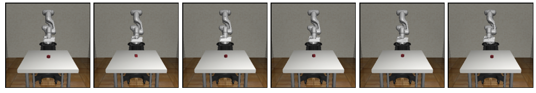
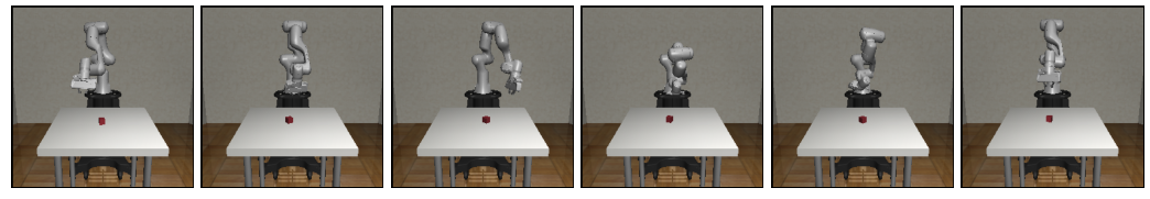
(a) Lift: Default initialization noise of 0.02 on the top, and initialization noise of 0.4 on the bottom.

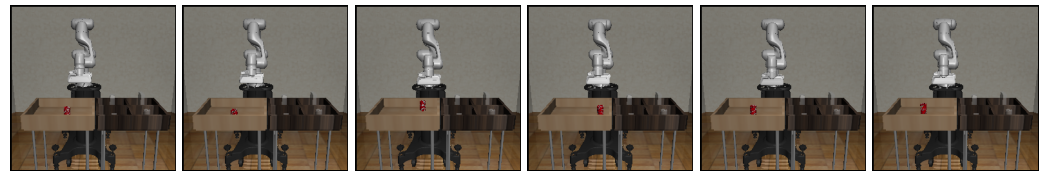
(b) PickPlaceCan: Default initialization of 0.02 on the top, and initialization noise of 0.4 on the bottom.

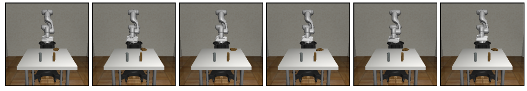
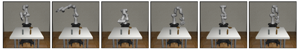
(c) NutAssemblySquare: Default initialization noise of 0.02 on the top, and initialization noise of 0.4 on the bottom.

Figure 7: Randomly sampled initial states for Robosuite environments. For all figures, the top row contains initial states with the default initialization noise of 0.02, while the bottom row contains initial states with initialization noise of 0.4. Notice in Figure 7(a) that with higher initialization noise, the robotic arm is less likely to start in positions directly above the block.

Appendix F Emergent Retrying & Videos

Figure 8 shows the retrying behavior of the POIR agent. We also attached multiple videos of the POIR-L2 agent (after 500k of finetuning) for the three environments. POIR-L2 is able to solve the task even when the initial position is very different from the one seen in the demonstrations. These videos also showcase the ability of POIR to retry the task until it is solved. In contrast, Ensemble BC is not able to retry the task and fail to solve it when the initial position is far from the ones in the demonstrations as shown in one of the attached videos. We also attached a video of DAC (after 5M steps) on Lift to showcase one failure mode of DAC: it keeps on re-trying the task without touching the object.

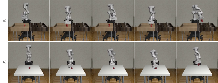
Figure 8: Visualization of retries from the POIR agent in a) PickPlaceCan and b) Lift. We select a trajectory in each environment and show a subset of frames in a chronological order. Notice that the arm attempts to grab the object, moves upwards without the object, and comes back to successfully grab the object. BC does not showcase this behavior.

References

- Pomerleau [1991] D. A. Pomerleau. Efficient training of artificial neural networks for autonomous navigation. Neural computation, 3(1):88–97, 1991.
- Zhang et al. [2018] T. Zhang, Z. McCarthy, O. Jow, D. Lee, X. Chen, K. Goldberg, and P. Abbeel. Deep imitation learning for complex manipulation tasks from virtual reality teleoperation. In 2018 IEEE International Conference on Robotics and Automation (ICRA), pages 5628–5635. IEEE, 2018.
- Zeng et al. [2020] A. Zeng, P. Florence, J. Tompson, S. Welker, J. Chien, M. Attarian, T. Armstrong, I. Krasin, D. Duong, V. Sindhwani, et al. Transporter networks: Rearranging the visual world for robotic manipulation. arXiv preprint arXiv:2010.14406, 2020.
- Florence et al. [2022] P. Florence, C. Lynch, A. Zeng, O. A. Ramirez, A. Wahid, L. Downs, A. Wong, J. Lee, I. Mordatch, and J. Tompson. Implicit behavioral cloning. In Conference on Robot Learning, pages 158–168. PMLR, 2022.
- Pomerleau [1989] D. A. Pomerleau. Alvinn: An autonomous land vehicle in a neural network. Technical report, CMU, 1989.
- Bojarski et al. [2016] M. Bojarski, D. Del Testa, D. Dworakowski, B. Firner, B. Flepp, P. Goyal, L. D. Jackel, M. Monfort, U. Muller, J. Zhang, et al. End to end learning for self-driving cars. arXiv preprint arXiv:1604.07316, 2016.
- Ross et al. [2011] S. Ross, G. Gordon, and D. Bagnell. A reduction of imitation learning and structured prediction to no-regret online learning. In Proceedings of the fourteenth international conference on artificial intelligence and statistics, pages 627–635. JMLR Workshop and Conference Proceedings, 2011.
- Thomas et al. [2019] P. S. Thomas, B. C. da Silva, A. G. Barto, S. Giguere, Y. Brun, and E. Brunskill. Preventing undesirable behavior of intelligent machines. Science, 366(6468):999–1004, 2019.
- Gottesman et al. [2018] O. Gottesman, F. Johansson, J. Meier, J. Dent, D. Lee, S. Srinivasan, L. Zhang, Y. Ding, D. Wihl, X. Peng, et al. Evaluating reinforcement learning algorithms in observational health settings. arXiv preprint arXiv:1805.12298, 2018.
- Bousmalis et al. [2018] K. Bousmalis, A. Irpan, P. Wohlhart, Y. Bai, M. Kelcey, M. Kalakrishnan, L. Downs, J. Ibarz, P. Pastor, K. Konolige, et al. Using simulation and domain adaptation to improve efficiency of deep robotic grasping. In 2018 IEEE international conference on robotics and automation (ICRA), pages 4243–4250. IEEE, 2018.
- Kalashnikov et al. [2018] D. Kalashnikov, A. Irpan, P. Pastor, J. Ibarz, A. Herzog, E. Jang, D. Quillen, E. Holly, M. Kalakrishnan, V. Vanhoucke, et al. Qt-opt: Scalable deep reinforcement learning for vision-based robotic manipulation. arXiv preprint arXiv:1806.10293, 2018.
- Ho and Ermon [2016] J. Ho and S. Ermon. Generative adversarial imitation learning. Advances in neural information processing systems, 29:4565–4573, 2016.
- Abbeel and Ng [2004] P. Abbeel and A. Y. Ng. Apprenticeship learning via inverse reinforcement learning. In Proceedings of the twenty-first international conference on Machine learning, page 1, 2004.
- Reddy et al. [2019] S. Reddy, A. D. Dragan, and S. Levine. Sqil: Imitation learning via reinforcement learning with sparse rewards. arXiv preprint arXiv:1905.11108, 2019.
- Kostrikov et al. [2019] I. Kostrikov, K. K. Agrawal, D. Dwibedi, S. Levine, and J. Tompson. Discriminator-actor-critic: Addressing sample inefficiency and reward bias in adversarial imitation learning. arXiv preprint arXiv:1809.02925, 2019.
- Argenson and Dulac-Arnold [2020] A. Argenson and G. Dulac-Arnold. Model-based offline planning. In International Conference on Learning Representations, 2020.
- Kidambi et al. [2020] R. Kidambi, A. Rajeswaran, P. Netrapalli, and T. Joachims. Morel: Model-based offline reinforcement learning. In NeurIPS, 2020.
- Yu et al. [2020] T. Yu, G. Thomas, L. Yu, S. Ermon, J. Y. Zou, S. Levine, C. Finn, and T. Ma. Mopo: Model-based offline policy optimization. Advances in Neural Information Processing Systems, 33:14129–14142, 2020.
- Zhu et al. [2020] Y. Zhu, J. Wong, A. Mandlekar, and R. Martín-Martín. robosuite: A modular simulation framework and benchmark for robot learning. In arXiv preprint arXiv:2009.12293, 2020.
- Sutton and Barto [2018] R. S. Sutton and A. G. Barto. Reinforcement learning: An introduction. MIT press, 2018.
- Ghasemipour et al. [2020] S. K. S. Ghasemipour, R. Zemel, and S. Gu. A divergence minimization perspective on imitation learning methods. In Conference on Robot Learning, pages 1259–1277. PMLR, 2020.
- Lakshminarayanan et al. [2017] B. Lakshminarayanan, A. Pritzel, and C. Blundell. Simple and scalable predictive uncertainty estimation using deep ensembles. In Advances in neural information processing systems, pages 6402–6413, 2017.
- Nagabandi et al. [2020] A. Nagabandi, K. Konolige, S. Levine, and V. Kumar. Deep dynamics models for learning dexterous manipulation. In Conference on Robot Learning, pages 1101–1112, 2020.
- Chua et al. [2018] K. Chua, R. Calandra, R. McAllister, and S. Levine. Deep reinforcement learning in a handful of trials using probabilistic dynamics models. In Advances in Neural Information Processing Systems, pages 4754–4765, 2018.
- Sasaki and Yamashina [2020] F. Sasaki and R. Yamashina. Behavioral cloning from noisy demonstrations. In International Conference on Learning Representations, 2020.
- Rault et al. [1978] J. Rault, A. Richalet, J. Testud, and J. Papon. Model predictive heuristic control: application to industrial processes. Automatica, 14(5):413–428, 1978.
- Williams et al. [2015] G. Williams, A. Aldrich, and E. Theodorou. Model predictive path integral control using covariance variable importance sampling. arXiv preprint arXiv:1509.01149, 2015.
- Lutter et al. [2021] M. Lutter, L. Hasenclever, A. Byravan, G. Dulac-Arnold, P. Trochim, N. Heess, J. Merel, and Y. Tassa. Learning dynamics models for model predictive agents. arXiv preprint arXiv:2109.14311, 2021.
- Tassa et al. [2012] Y. Tassa, T. Erez, and E. Todorov. Synthesis and stabilization of complex behaviors through online trajectory optimization. In 2012 IEEE/RSJ International Conference on Intelligent Robots and Systems, pages 4906–4913. IEEE, 2012.
- Williams et al. [2017] G. Williams, N. Wagener, B. Goldfain, P. Drews, J. M. Rehg, B. Boots, and E. A. Theodorou. Information theoretic mpc for model-based reinforcement learning. In 2017 IEEE International Conference on Robotics and Automation (ICRA), pages 1714–1721. IEEE, 2017.
- Indyk and Motwani [1998] P. Indyk and R. Motwani. Approximate nearest neighbors: towards removing the curse of dimensionality. In Proceedings of the thirtieth annual ACM symposium on Theory of computing, pages 604–613, 1998.
- Guo et al. [2020] R. Guo, P. Sun, E. Lindgren, Q. Geng, D. Simcha, F. Chern, and S. Kumar. Accelerating large-scale inference with anisotropic vector quantization. In International Conference on Machine Learning, pages 3887–3896. PMLR, 2020.
- Dadashi et al. [2021] R. Dadashi, L. Hussenot, M. Geist, and O. Pietquin. Primal wasserstein imitation learning. In ICLR 2021-Ninth International Conference on Learning Representations, 2021.
- Brantley et al. [2019] K. Brantley, W. Sun, and M. Henaff. Disagreement-regularized imitation learning. In International Conference on Learning Representations, 2019.
- Mandlekar et al. [2021] A. Mandlekar, D. Xu, J. Wong, S. Nasiriany, C. Wang, R. Kulkarni, L. Fei-Fei, S. Savarese, Y. Zhu, and R. Martín-Martín. What matters in learning from offline human demonstrations for robot manipulation. arXiv preprint arXiv:2108.03298, 2021.
- Mandlekar et al. [2018] A. Mandlekar, Y. Zhu, A. Garg, J. Booher, M. Spero, A. Tung, J. Gao, J. Emmons, A. Gupta, E. Orbay, et al. Roboturk: A crowdsourcing platform for robotic skill learning through imitation. In Conference on Robot Learning, pages 879–893. PMLR, 2018.
- Orsini et al. [2021] M. Orsini, A. Raichuk, L. Hussenot, D. Vincent, R. Dadashi, S. Girgin, M. Geist, O. Bachem, O. Pietquin, and M. Andrychowicz. What matters for adversarial imitation learning? arXiv preprint arXiv:2106.00672, 2021.
- Kostrikov et al. [2019] I. Kostrikov, O. Nachum, and J. Tompson. Imitation learning via off-policy distribution matching. arXiv preprint arXiv:1912.05032, 2019.
- Schulman et al. [2017] J. Schulman, F. Wolski, P. Dhariwal, A. Radford, and O. Klimov. Proximal policy optimization algorithms. arXiv preprint arXiv:1707.06347, 2017.
- Ross and Bagnell [2010] S. Ross and D. Bagnell. Efficient reductions for imitation learning. In Proceedings of the thirteenth international conference on artificial intelligence and statistics, pages 661–668. JMLR Workshop and Conference Proceedings, 2010.
- Ng et al. [2000] A. Y. Ng, S. J. Russell, et al. Algorithms for inverse reinforcement learning. In Icml, volume 1, page 2, 2000.
- Lee et al. [2018] K. Lee, K. Saigol, and E. A. Theodorou. Safe end-to-end imitation learning for model predictive control. ArXiv, abs/1803.10231, 2018.
- Silvério et al. [2019] J. Silvério, Y. Huang, F. J. Abu-Dakka, L. Rozo, and D. G. Caldwell. Uncertainty-aware imitation learning using kernelized movement primitives. In 2019 IEEE/RSJ International Conference on Intelligent Robots and Systems (IROS), pages 90–97. IEEE, 2019.
- Cui et al. [2019] Y. Cui, D. Isele, S. Niekum, and K. Fujimura. Uncertainty-aware data aggregation for deep imitation learning. In 2019 International Conference on Robotics and Automation (ICRA), pages 761–767. IEEE, 2019.
- Di Palo and Johns [2020] N. Di Palo and E. Johns. Safari: Safe and active robot imitation learning with imagination. arXiv preprint arXiv:2011.09586, 2020.
- Baram et al. [2017] N. Baram, O. Anschel, I. Caspi, and S. Mannor. End-to-end differentiable adversarial imitation learning. In International Conference on Machine Learning, pages 390–399. PMLR, 2017.
- Kim and Park [2018] K.-E. Kim and H. S. Park. Imitation learning via kernel mean embedding. In Thirty-Second AAAI Conference on Artificial Intelligence, 2018.
- Wang et al. [2019] R. Wang, C. Ciliberto, P. V. Amadori, and Y. Demiris. Random expert distillation: Imitation learning via expert policy support estimation. In International Conference on Machine Learning, pages 6536–6544. PMLR, 2019.
- Kelly et al. [2019] M. Kelly, C. Sidrane, K. Driggs-Campbell, and M. J. Kochenderfer. Hg-dagger: Interactive imitation learning with human experts. In 2019 International Conference on Robotics and Automation (ICRA), pages 8077–8083. IEEE, 2019.
- Yu et al. [2021] T. Yu, A. Kumar, R. Rafailov, A. Rajeswaran, S. Levine, and C. Finn. Combo: Conservative offline model-based policy optimization. In Self-Supervision for Reinforcement Learning Workshop-ICLR 2021, 2021.
- Rafailov et al. [2021] R. Rafailov, T. Yu, A. Rajeswaran, and C. Finn. Offline reinforcement learning from images with latent space models. In Learning for Dynamics and Control, pages 1154–1168. PMLR, 2021.
- Zhan et al. [2021] X. Zhan, X. Zhu, and H. Xu. Model-based offline planning with trajectory pruning. arXiv e-prints, pages arXiv–2105, 2021.
- Osa et al. [2018] T. Osa, J. Pajarinen, G. Neumann, J. A. Bagnell, P. Abbeel, J. Peters, et al. An algorithmic perspective on imitation learning. Foundations and Trends in Robotics, 7(1-2):1–179, 2018.
- Englert et al. [2013] P. Englert, A. Paraschos, M. P. Deisenroth, and J. Peters. Probabilistic model-based imitation learning. Adaptive Behavior, 21(5):388–403, 2013.
- Qi et al. [2022] C. Qi, P. Abbeel, and A. Grover. Imitating, fast and slow: Robust learning from demonstrations via decision-time planning. arXiv preprint arXiv:2204.03597, 2022.
- Rhinehart et al. [2018] N. Rhinehart, R. McAllister, and S. Levine. Deep imitative models for flexible inference, planning, and control. arXiv preprint arXiv:1810.06544, 2018.
- Tigas et al. [2019] P. Tigas, A. Filos, R. McAllister, N. Rhinehart, S. Levine, and Y. Gal. Robust imitative planning: Planning from demonstrations under uncertainty. In NeurIPS 2019 Workshop on Machine Learning for Autonomous Driving, 2019.
- Filos et al. [2020] A. Filos, P. Tigkas, R. McAllister, N. Rhinehart, S. Levine, and Y. Gal. Can autonomous vehicles identify, recover from, and adapt to distribution shifts? In International Conference on Machine Learning, pages 3145–3153. PMLR, 2020.
- Lin et al. [2021] H. Lin, B. Li, X. Zhou, J. Wang, and M. Q.-H. Meng. No need for interactions: Robust model-based imitation learning using neural ode. arXiv preprint arXiv:2104.01390, 2021.
- Wu et al. [2020] A. Wu, A. Piergiovanni, and M. S. Ryoo. Model-based behavioral cloning with future image similarity learning. In Conference on Robot Learning, pages 1062–1077. PMLR, 2020.
- Richalet et al. [1978] J. Richalet, A. Rault, J. Testud, and J. Papon. Model predictive heuristic control. Automatica (journal of IFAC), 14(5):413–428, 1978.
- Kirk et al. [2021] R. Kirk, A. Zhang, E. Grefenstette, and T. Rocktäschel. A survey of generalisation in deep reinforcement learning. arXiv preprint arXiv:2111.09794, 2021.
- Lynch et al. [2020] C. Lynch, M. Khansari, T. Xiao, V. Kumar, J. Tompson, S. Levine, and P. Sermanet. Learning latent plans from play. In Conference on Robot Learning, pages 1113–1132. PMLR, 2020.
- Jang et al. [2021] E. Jang, A. Irpan, M. Khansari, D. Kappler, F. Ebert, C. Lynch, S. Levine, and C. Finn. Bc-z: Zero-shot task generalization with robotic imitation learning. In 5th Annual Conference on Robot Learning, 2021.
- James et al. [2018] S. James, M. Bloesch, and A. J. Davison. Task-embedded control networks for few-shot imitation learning. In Conference on Robot Learning, pages 783–795. PMLR, 2018.
- Finn et al. [2017] C. Finn, T. Yu, T. Zhang, P. Abbeel, and S. Levine. One-shot visual imitation learning via meta-learning. In Conference on Robot Learning, pages 357–368. PMLR, 2017.
- Yu et al. [2018] T. Yu, C. Finn, A. Xie, S. Dasari, T. Zhang, P. Abbeel, and S. Levine. One-shot imitation from observing humans via domain-adaptive meta-learning. arXiv preprint arXiv:1802.01557, 2018.
- Tobin et al. [2017] J. Tobin, R. Fong, A. Ray, J. Schneider, W. Zaremba, and P. Abbeel. Domain randomization for transferring deep neural networks from simulation to the real world. In 2017 IEEE/RSJ international conference on intelligent robots and systems (IROS), pages 23–30. IEEE, 2017.
- Mehta et al. [2020] B. Mehta, M. Diaz, F. Golemo, C. J. Pal, and L. Paull. Active domain randomization. In Conference on Robot Learning, pages 1162–1176. PMLR, 2020.
- Xing et al. [2021] E. Xing, A. Gupta, S. Powers, and V. Dean. Kitchenshift: Evaluating zero-shot generalization of imitation-based policy learning under domain shifts. In NeurIPS 2021 Workshop on Distribution Shifts: Connecting Methods and Applications, 2021.
- Chebotar et al. [2021] Y. Chebotar, K. Hausman, Y. Lu, T. Xiao, D. Kalashnikov, J. Varley, A. Irpan, B. Eysenbach, R. Julian, C. Finn, et al. Actionable models: Unsupervised offline reinforcement learning of robotic skills. arXiv preprint arXiv:2104.07749, 2021.
- Cobbe et al. [2019] K. Cobbe, O. Klimov, C. Hesse, T. Kim, and J. Schulman. Quantifying generalization in reinforcement learning. In International Conference on Machine Learning, pages 1282–1289. PMLR, 2019.
- Hafner et al. [2019a] D. Hafner, T. Lillicrap, J. Ba, and M. Norouzi. Dream to control: Learning behaviors by latent imagination. arXiv preprint arXiv:1912.01603, 2019a.
- Hafner et al. [2019b] D. Hafner, T. Lillicrap, I. Fischer, R. Villegas, D. Ha, H. Lee, and J. Davidson. Learning latent dynamics for planning from pixels. In International Conference on Machine Learning, pages 2555–2565, 2019b.
- Kingma and Ba [2014] D. P. Kingma and J. Ba. Adam: A method for stochastic optimization. arXiv preprint arXiv:1412.6980, 2014.
- Hoffman et al. [2020] M. Hoffman, B. Shahriari, J. Aslanides, G. Barth-Maron, F. Behbahani, T. Norman, A. Abdolmaleki, A. Cassirer, F. Yang, K. Baumli, et al. Acme: A research framework for distributed reinforcement learning. arXiv preprint arXiv:2006.00979, 2020.