Persistence K-theory

Abstract.

This paper studies the basic $K$-theoretic properties of a triangulated persistence category (TPC). This notion was introduced in [10] and it is a type of category that can be viewed as a refinement of a triangulated category in the sense that the morphisms sets of a TPC are persistence modules. We calculate the $K$-groups in some basic examples and discuss an application to Fukaya categories and to the topology of exact Lagrangian submanifolds.

1. Introduction

The main aim of the paper is to study $K$-theoretic properties of triangulated persistence categories (TPCs) and provide some applications of these properties in the setting of symplectic topology. We recall from [10] (or its earlier version [9]) that a TPC is, roughly, a persistence category $\mathcal{C}$ - that is a category with morphisms that are persistence modules $\hom_{\mathcal{C}}(A,B)=\{\hom_{\mathcal{C}}^{\alpha}(A,B)\}_{\alpha\in\mathbb{R}}$, with composition compatible with the persistence structure - such that the $0$-level category $\mathcal{C}_{0}$, with the same objects as $\mathcal{C}$ but with only the $0$-level morphisms $\hom_{\mathcal{C}_{0}}(-,-)=\hom_{C}^{0}(-,-)$, is triangulated. The full definition and all relevant notions are recalled in §2.4. The fundamental property of such a TPC $\mathcal{C}$ is that the $\infty$-level category, $\mathcal{C}_{\infty}$, again with the same objects as $\mathcal{C}$ but with morphisms the $\infty$-limit of $\hom_{C}(-,-)$ is also triangulated and that its exact triangles each carry a weight $r\geq 0$. Using this weight one can define a family of fragmentation pseudo-distances on the objects of $\mathcal{C}$, by taking into account the weights required to decompose objects by means of exact triangles.

The basic $K$-theoretic constructions associated to a TPC $\mathcal{C}$ appear in Section 3. Recall that the Grothendieck group $K(\mathcal{D})$ of a triangulated category $\mathcal{D}$ is defined as the abelian group freely generated by the objects of the category modulo the relations $B=A+C$ for each exact triangle $A\to B\to C\to TA$ in $\mathcal{D}$, where $T$ is the translation functor of $\mathcal{D}$.

Returning to the triangulated persistence category $\mathcal{C}$, we define its $K$-group by

$$K(\mathcal{C}):=K(\mathcal{C}_{0})~{}.~{}$$

This is a linearization of $\mathcal{C}$ that transforms iterated cones involving only $0$-weight triangles in linear relations. Thus the $K$-class $[X]\in K(\mathcal{C})$ of an object $X\in\mathrm{Obj}(\mathcal{C})$ can be viewed as an algebraic invariant of $X$ in the rough sense that it is invariant under the $0$-isomorphisms (see Lemma 3.2.2). At the same time, because higher weight triangles are not used in the quotient giving $K(\mathcal{C})$, this $K$-group continues to carry relevant metric information.

The more precise aim of the paper is to understand more of the structure of this group, in particular the interplay between the algebraic and metric aspects.

A first structural result relates $K(\mathcal{C})$ to the $K$-group of the $\infty$-level of $\mathcal{C}$, $K_{\infty}(\mathcal{C}):=K(\mathcal{C}_{\infty})$. We notice in §3 that there exists a long exact sequence of $\Lambda_{P}$-modules:

$$0\to{\rm Tor}K(\mathcal{C})\to K(\mathscr{A}\mathcal{C})\to K(\mathcal{C})\to K_{\infty}(\mathcal{C})\to 0.$$ (1)

Here $\Lambda_{P}$ is the universal Novikov polynomial ring with integral coefficients (we recall its definition in §2.1), and the $K$-groups of TPC’s are naturally $\Lambda_{P}$-modules. The category $\mathcal{AC}$ is the full subcategory of $\mathcal{C}$ whose objects are the objects of $\mathcal{C}$ that are isomorphic to $0$ in $\mathcal{C}_{\infty}$, this is called the acyclic subcategory of $\mathcal{C}$. This $\mathscr{A}\mathcal{C}$ is also a TPC thus the $K$-group, $K(\mathscr{A}\mathcal{C}):=K(\mathscr{A}\mathcal{C}_{0})$, is defined as above. The term ${\rm Tor}K(-)$ is a torsion type functor. To put this in some perspective, recall from [10] that $\mathcal{C}_{\infty}$ is the Verdier localization $\mathcal{C}_{0}/\mathcal{AC}_{0}$.

In Section 4 we compute the relevant $K$-groups for categories of filtered chain complexes. We will focus in this introduction on just one example, $\mathcal{C}^{\text{fg}}=H_{0}(\mathscr{F}\mathbf{Ch}^{\text{fg}})$, the homotopy category of finitely generated, filtered chain complexes. Filtered chain complexes (of different types) provide the most common examples of TPCs. Additionally, these examples are also universal in certain ways. For instance, we show that for $\mathcal{C}=\mathcal{C}^{\text{fg}}$ the exact sequence (1) can be identified with the following one:

$$0\to 0\to\Lambda_{P}^{(0)}\to\Lambda_{P}\to\mathbb{Z}\to 0,$$

where $\Lambda_{P}^{(0)}\subset\Lambda_{P}$ is the ideal consisting of the Novikov polynomials $P(t)$ that vanish at $t=1$, i.e. $P(1)=0$. The most interesting part of the identification of (1) with the latter sequence is the isomorphism

$$K(\mathcal{C}^{\text{fg}})\xrightarrow{\;\;\cong\;\;}\Lambda_{P}$$ (2)

which shows that, in this case, the $\Lambda_{P}$-module $K(\mathcal{C})$ coincides with $\Lambda_{P}$ itself. We will denote this isomorphism by $\lambda$ and outline its definition soon. The isomorphism $K_{\infty}(\mathcal{C}^{\text{fg}})\xrightarrow{\;\;\cong\;\;}\mathbb{Z}$ is induced by the Euler characteristic.

The isomorphism $\lambda:K(\mathcal{C}^{\text{fg}})\xrightarrow{\;\;\cong\;\;}\Lambda_{P}$ is induced by the following way to associate a polynomial to a filtered, finitely generated chain complex $C$. First associate to $C$ its (graded) persistence homology $H_{*}(C)$ (see §2.2 for a rapid review of the definitions). Then associate to $H_{*}(C)$ its graded barcode $\mathcal{B}_{H_{*}(C)}$. This consists of a finite collection of intervals (a.k.a. bars) of the form $[a,b)$ and $[c,\infty)$, where each interval has a certain degree in $\mathbb{Z}$. To an interval $[a,b)$ of degree $k$ we associate the polynomial $(-1)^{k}(t^{a}-t^{b})\in\Lambda_{P}$, and to an interval $[c,\infty)$ of degree $k$ we associate $(-1)^{k}t^{c}$. Finally, we sum up the previously defined polynomials over each interval in the graded barcode $\mathcal{B}_{H_{*}(C)}$ and obtain a Novikov polynomial $\lambda_{H_{*}(C)}$. The map $C\longmapsto\lambda_{H_{*}(C)}\in\Lambda_{P}$ induces the isomorphism $\lambda$. An additional point to note here is that $K(\mathcal{C})$ is a $\Lambda_{P}$-algebra in case $\mathcal{C}$ has a monoidal structure (as defined in §3.3). This is the case for $\mathcal{C}^{\text{fg}}$, the monoidal operation being the tensor product, and the isomorphism $\lambda$ is a ring isomorphism.

In Section 5 we investigate a natural way to associate to a graded persistence module, or to a barcode, a real function. As a by-product we reinterpret the map $C\to[C]\in K(\mathcal{C}^{\text{fg}})$ that associates to a filtered chain complex its $K$-class as a filtered Euler characteristic. Given a persistence module $M=\{M^{\alpha}\}_{\alpha\in\mathbb{R}}$ consider the integral-valued function $\sigma_{M}(\alpha)=\dim(M^{\alpha})$. With the definition of persistence modules considered in this paper (see 2.2), and assuming some finite type constraints, $\sigma_{M}:\mathbb{R}\to\mathbb{R}$ is a bounded step function belonging to a group of such functions, denoted by $LC_{B}$ and defined in §5.1. If $M_{\bullet}$ is a graded persistence module consisting of persistence modules $M_{i}$ for each degree $i$ it is natural to consider the Euler characteristic function $\bar{\chi}_{M_{\bullet}}\in LC_{B}$, $\bar{\chi}_{M_{\bullet}}=\sum_{k}(-1)^{k}\sigma_{M_{k}}$. We show that $LC_{B}$ admits a remarkable ring structure based on convolution of functions and, with this ring structure, it is isomorphic to the ring $\Lambda_{P}$. Moreover, under this ring isomorphism $LC_{B}\cong\Lambda_{P}$, the map $M_{\bullet}\to\bar{\chi}_{M_{\bullet}}\in LC_{B}$ is another expression of $\lambda$ from (2). This chapter also contains - in Proposition 5.3.1 - a persistence version of the Morse inequalities as well as an application to counting bars, in Corollary 5.3.4.

In Section 6 we return to the general setting and consider a triangulated persistence category $\mathcal{C}$. Under some finite type constraints we show that there exists a bilinear pairing

$$\kappa:\overline{K(\mathcal{C})}\otimes_{\Lambda_{P}}K(\mathcal{C})\to\Lambda_{P}$$ (3)

Here $\overline{K(\mathcal{C})}$ is the same abelian group as $K(\mathcal{C})$ but with the $\Lambda_{P}$-module structure $\bar{\cdot}$ such that $t\,\bar{\cdot}\,x=t^{-1}\cdot x$ where $\cdot$ is the module structure on $K(\mathcal{C})$. The pairing $\kappa$ is induced by the map that associates to a pair of objects $X,Y$ the Novikov polynomial $\lambda_{\hom_{C}(X,T^{\ast}(Y))}$ where $\hom_{\mathcal{C}}(X,T^{\ast}(Y))$ is the graded persistence module having $\hom_{\mathcal{C}}(X,T^{i}Y)$ in degree $i$ (recall that $T$ is the translation functor in $\mathcal{C}_{0}$). In view of the discussion above, notice that $\kappa$ can be viewed as an Euler pairing. The pairing is particularly simple in the case of the category $\mathcal{C}^{\text{fg}}$. Using the identification $K(\mathcal{C}^{\text{fg}})\cong\Lambda_{P}$, we have $k(P,Q)(t)=P(t^{-1})Q(t)$ for any two polynomials $P,Q\in\Lambda_{P}$. There are conditions - of Calabi-Yau duality type - implying that the pairing $\kappa$ is skew symmetric in the sense that $\kappa(x,y)(t)=\kappa(y,x)(t^{-1})$. These conditions are satisfied for the category $\mathcal{C}^{\text{fg}}$.

Section 7 is dedicated to analyzing “measurements” on $K$-groups. We see that fragmentation pseudo-distances on the objects of a TPC $\mathcal{C}$ can be used to define non-trivial group semi-norms on $K(\mathcal{C})$. We then discuss other ways to extract quantitative information from barcodes by using their representation in $LC_{B}$.

Section 8 deals with applications to symplectic topology. We discuss some results indicating that the pairing $\kappa$ defined on the $K$-group of the triangulated persistence Fukaya category introduced in Chapter 3 of [10] distinguishes, in a quantitative way, embedded from immersed Lagrangians. The main results are in Corollary 8.1.2 and Theorem 8.1.4. The corollary shows that the pairing $\kappa(A,A)$, where $A$ is the $K$-class of an embedded Lagrangian, is a constant Novikov polynomial equal to the Euler characteristic of the Lagrangian (up to sign). The theorem provides a way to estimate the minimal “energy” required to transform certain immersed Lagrangians into embedded ones. The estimate is somewhat subtle as it involves also estimates on the number of bars in certain associated barcodes that are deduced from the persistence Morse inequalities in §5.

2. Prerequisites

We list here some of the conventions used further in the paper and we recall some of the notions required to make the reading of this paper more accessible.

2.1. Novikov rings

We will use the following versions of the Novikov ring. We denote by

$$\Lambda=\left\{\sum_{k=0}^{\infty}n_{k}t^{a_{k}}\,\bigg{|}\,n_{k}\in\mathbb{Z},a_{k}\in\mathbb{R},\lim_{k\to\infty}a_{k}=\infty\right\}$$ (4)

the Novikov ring with coefficients in $\mathbb{Z}$ (and formal variable $t$), endowed with the standard multiplication. Denote also by $\Lambda_{P}\subset\Lambda$ the subring of Novikov polynomials, whose elements consist of finite sums $\sum n_{k}t^{a_{k}}\in\Lambda$.

2.2. Persistence modules

The bibliography on persistence modules contains a large number of variants of the definition. We fix here the setting that we will use in this paper.

A persistence module $M$ is a family of vector spaces over the field $\mathbf{k}$, indexed by the reals, $M=\{M^{s}\}_{s\in\mathbb{R}}$, together with maps $i_{s,t}:M^{s}\to M^{t}$ for all $s\leq t$ satisfying $i_{t,r}\circ i_{s,t}=i_{s,r}$ for all $s\leq t\leq r\in\mathbb{R}$ and $i_{s,s}=\mathds{1}$ for any $s\in\mathbb{R}$. We will always assume that the following three conditions apply to the persistence modules $M$ considered here.

• (lower semi-continuity) For any $s\in\mathbb{R}$ and any $t\geq s$ sufficiently close to $s$, the map $i_{s,t}:M^{s}\to M^{t}$ is an isomorphism.

• (lower bounded) For $s$ sufficiently small we have $M^{s}=0$.

• (tame) For every $s\in\mathbb{R}$,  we have

  $$\dim_{\mathbf{k}}(M^{s})<\infty.$$ (5)

We will often use graded persistence modules. Namely, $M_{\bullet}$ is a graded persistence module if $M_{\bullet}=\{M_{i}\}_{i\in\mathbb{Z}}$ is a sequence of persistence modules indexed by $\mathbb{Z}$ with the index indicating the degree. The tameness condition in this case becomes:

$$\mathrm{for\ every}\ s\in\mathbb{R},\ \dim_{\mathbf{k}}(\oplus_{i\in\mathbb{Z}}M_{i}^{s})<\infty~{}.~{}$$ (6)

The homology of filtered chain complexes provides some of the most typical examples of persistence modules. For our purposes here, a filtered chain complex is a triple $(C_{*},\partial,\ell)$ where $(C_{*},\partial)$ is a chain complex and $\ell:\oplus_{i}C_{i}\to\mathbb{R}\cup\{-\infty\}$ is a filtration function (see [34, Definition 2.2]). In particular, $\partial$ and $\ell$ are compatible in the sense that

$$\ell(\partial x)\leq\ell(x)\,\,\,\,\,\mbox{for any $x\in C_{*}$}.$$

It follows that for any $r\in\mathbb{R}$ the truncation $(C_{*}^{\leq r},\partial)$ where $C_{*}^{\leq r}=\{x\in C\ |\ \ell(x)\leq r\}$ is a well-defined chain complex. The same holds also for the “strict” truncations $C_{*}^{<r}$.

We will consider mainly two types of filtered chain complexes:

• finitely generated - chain complexes for which the total space $\oplus_{k\in\mathbb{Z}}C_{k}$ is finite dimensional, and moreover $C_{\ast}^{\leq r}=0$ for $r$ sufficiently small.

• tame - chain complexes such that $\oplus_{k\in\mathbb{Z}}C^{\leq r}_{k}$ is finite dimensional for all $r\in\mathbb{R}$, and moreover $C_{\ast}^{\leq r}=0$ for $r$ sufficiently small.

If a filtered chain complex $C$ is tame, then $\{C_{\ast}^{\leq r}\}_{r\in\mathbb{R}}$ forms a graded persistence module in the class discussed above. Moreover, the homology of these truncations, $\{H_{\ast}(C^{\leq r})\}_{r\in\mathbb{R}}$, also forms a graded persistence module in the same class. We will denote this persistence module by $H_{*}(C)$.

2.3. Barcodes

In this paper we will use the following version of barcodes. A barcode $\mathcal{B}=\{(I_{j},m_{j})\}_{j\in\mathcal{J}}$ is a collection of pairs consisting of intervals $I_{j}\subset\mathbb{R}$ and positive integers $m_{j}\in\mathbb{Z}_{>0}$, indexed by a set $\mathcal{J}$, and satisfying the following admissibility conditions:

1. $\mathcal{J}$ is assumed to be either finite or $\mathcal{J}=\mathbb{Z}_{\geq 0}$.

2. Each interval $I_{j}$ is of the type $I_{j}=[a_{j},b_{j})$, with $-\infty<a_{j}<b_{j}\leq\infty$.

3. In case $\mathcal{J}=\mathbb{Z}_{\geq 0}$ we assume that $a_{j}\rightarrow\infty$ as $j\rightarrow\infty$.

The intervals $I_{j}$ are called bars and for each $j$, $m_{j}$ is called the multiplicity of the bar $I_{j}$.

To every barcode $\mathcal{B}$ we can associate a persistence module in the following way. For an interval $I=[a,b)$ as above, denote by $V(I)$ the persistence module defined by

$$V^{s}(I)=\begin{cases}\mathbf{k},&\text{if $s\in I$;}\\ 0,&\text{if $s\notin I$,}\end{cases}$$ (7)

and with persistence maps $i_{s,t}:V^{s}(I)\longrightarrow V^{t}(I)$ being the identity map $\textnormal{id}_{\mathbf{k}}$ whenever $s,t\in I$. We call $V(I)$ the interval module corresponding to $I$.

By taking direct sums we associate to every barcode $\mathcal{B}=\{(I_{j},n_{j})\}_{j\in\mathcal{J}}$ a persistence module, as follows:

$$V(\mathcal{B}):=\bigoplus_{j\in\mathcal{J}}V(I_{j})^{\oplus m_{j}}.$$ (8)

It is easy to see that $V(\mathcal{B})$ satisfies the conditions in §2.2. Conversely, it is well known that this construction can be reversed. More precisely, with the conventions from §2.2, we have that for every persistence module $M$ there exists a unique barcode $\mathcal{B}$ as above and such that $M\cong V(\mathcal{B})$. In other words, barcodes classify isomorphism types of persistence modules. See [34, 27] for more details. We will denote the barcode corresponding to a persistence module $M$ by $\mathcal{B}_{M}$.

We will need also the notion of graded barcodes. By this we mean a sequence of barcodes $\mathcal{B}=\{\mathcal{B}_{i}\}_{i\in\mathbb{Z}}$ indexed by the integers and satisfying the following additional assumption. Denote by $\mathcal{B}^{\text{tot}}$ the union of all the intervals in all the $\mathcal{B}_{i}$’s, together with their multiplicities and adding up multiplicities whenever bars from different $\mathcal{B}_{i}$’s coincide). We assume that $\mathcal{B}^{\text{tot}}$ is an admissible barcode, in the sense that all the multiplicities appearing in it are finite, and moreover that it satisfies the admissibility conditions (1), (2), (3) above.

We will often regard a single (ungraded) barcode $\mathcal{B}$ as a graded one, simply by placing it in degree $0$.

Let $\mathcal{B}=\{(I_{j},m_{j})\}_{j\in\mathcal{J}}$ be an ungraded barcode. We associate to $\mathcal{B}$ an element $\lambda_{\mathcal{B}}\in\Lambda$ of the Novikov ring as follows:

$$\lambda_{\mathcal{B}}:=\sum_{j\in\mathcal{J}}m_{j}\lambda_{I_{j}},$$ (9)

where

$$\lambda_{I_{j}}:=\begin{cases}t^{a_{j}}-t^{b_{j}},&\text{if $I_{j}=[a_{j},b_{j})$;}\\ t^{a_{j}},&\text{if $I_{j}=[a_{j},\infty)$.}\end{cases}$$ (10)

Let $M$ be a persistence module with barcode $\mathcal{B}_{M}$. Applying the construction above, we obtain an element of the Novikov ring

$$\lambda_{M}:=\lambda_{\mathcal{B}_{M}}\in\Lambda.$$ (11)

The definition of $\lambda_{M}$ can be extended to the graded case. Namely, let $M_{\bullet}=\{M_{i}\}_{i\in\mathbb{Z}}$ be a graded persistence module. Assume further the tameness condition in (6), then define:

$$\lambda_{M_{\bullet}}:=\sum_{i\in\mathbb{Z}}(-1)^{i}\lambda_{M_{i}}\ \in\ \Lambda~{}.~{}$$ (12)

A similar definition is available for graded barcodes.

2.4. Triangulated persistence categories

Triangulated persistence categories were introduced in [9, 10]. We will only roughly review here some of the basics to make the current paper more accessible.

A TPC is a category $\mathcal{C}$ with four properties summarized below (we refer to [10] for the full definitions).

• $\mathcal{C}$ is a persistence category. This means that for each two objects $A,B$ of $\mathcal{C}$, the morphisms $\hom_{\mathcal{C}}(A,B)$ form a persistence module $\{\hom_{\mathcal{C}}^{s}(A,B)\}_{s\in\mathbb{R}}$ and that composition of morphisms is compatible with the persistence structure in the obvious way. In the current paper we will assume that these persistence modules are always lower-bounded and lower-semicontinuous - see §2.2.

• $\mathcal{C}$ carries a “shift functor” $\Sigma$. This is a structure composed of shift functors $\Sigma^{r}:\mathcal{C}\to\mathcal{C}$ where $\Sigma^{r}\circ\Sigma^{s}=\Sigma^{r+s}$ for all $r,s\in\mathbb{R}$ and $\Sigma^{0}=\mathds{1}$ that are compatible with the persistence structure, and of natural isomorphisms $\eta_{r,s}:\Sigma^{r}\to\Sigma^{s}$ satisfying some natural compatibility relations and with $\eta_{r,r}=id$, $\eta_{r,s}\in\hom^{s-r}(-,-)$.

  To keep an example in mind, the simplest TPC is the (homotopy) category of filtered chain complexes. In that case $\Sigma^{r}C$ is obtained from the filtered chain complex $C$ by shifting the filtration up by $r$ and the natural transformation $\Sigma^{r}C\stackrel{{\scriptstyle\eta_{r,s}}}{{\longrightarrow}}\Sigma^{s}C$ is the identity at the vector space level, when the filtration is forgotten.

• The category $\mathcal{C}_{0}$ with the same objects as $\mathcal{C}$ and whose morphism are the $0$-level morphisms of $\mathcal{C}$, $\hom_{\mathcal{C}}^{0}(-,-)$, is triangulated, $\Sigma^{r}$ is a triangulated functor (on $\mathcal{C}_{0}$), and $\eta_{r,s}$ are compatible with the additive structure on $\mathcal{C}_{0}$. Note that being triangulated, $\mathcal{C}_{0}$ has a translation functor $T$. This functor should not be confused with the shift functor $\Sigma$ which has to do with shifting the persistence level. (Unfortunately the names “shift” and “translation” functor are both used for the same thing in the context of triangulated categories, often related to a shift or translation in grading. However in our framework these two notions are absolutely different from each other.)

• To formulate the last property that characterizes a TPC we need a couple more notions that will also be useful later in the paper. We say that $f,g\in\hom_{\mathcal{C}}^{s}(A,B)$ are $r$-equivalent if $i_{s,s+r}(f-g)=0$. Here $i_{s,s+r}:\hom^{s}(-,-)\to\hom^{s+r}(-,-)$ are the persistence structural maps. We write $f\simeq_{r}g$. An object $K$ is called $r$-acyclic for some $r\geq 0$ if $\mathds{1}_{K}\simeq_{r}0$.

  For all $r\geq 0$, the natural transformation $\eta_{r,0}:\Sigma^{r}\to\Sigma^{0}=\mathds{1}$, specialized to $X\in\text{Obj}(\mathcal{C})$ belongs to $\hom^{-r}(\Sigma^{r}X,X)$ so we can apply to it $i_{-r,0}:\hom^{-r}(\Sigma^{r}X,X)\to\hom^{0}(\Sigma^{r}X,X)$. The result is denoted by $\eta_{r}=i_{-r,0}(\eta_{r,0})$ and thus $\eta_{r}\in\hom_{\mathcal{C}_{0}}$.

  Then the fourth property that defines a TPC is the following: For each $r\geq 0$ and object $X$ of $\mathcal{C}$ there is an exact triangle in $\mathcal{C}_{0}$

  $$\Sigma^{r}X\stackrel{{\scriptstyle\eta_{r}}}{{\longrightarrow}}X\to K\to T\Sigma^{r}X$$

  with $K$ being $r$-acyclic.

Definition 2.4.1.

(a) A triangulated persistence category $\mathcal{C}$ is called tame if, for any two objects $A,B\in\mathrm{Obj}(\mathcal{C})$, the persistence module $\hom_{\mathcal{C}}(A,B)$ satisfies tame condition (5) and is called of finite type if the barcode of the persistence module $\hom_{\mathcal{C}}(A,B)$ has only finitely many bars.

(b) The triangulated persistence category $\mathcal{C}$ is called bounded if for every two objects $X,Y\in\mathrm{Obj}(\mathcal{C})$ there exists $l\in\mathbb{N}$ with the property that $\hom_{\mathcal{C}}(X,T^{i}Y)=0$ for every $|i|\geq l$. Here, $T$ is the translation functor of the triangulated category $\mathcal{C}_{0}$.

Obviously, if a TPC is tame and $X,Y\in\mathrm{Obj}(\mathcal{C})$ are two of its objects, then

$$\lambda_{\hom_{\mathcal{C}}(X,Y)}\in\Lambda$$

is well-defined as an element in the Novikov ring $\Lambda$. Further, given $X,Y\in\mathrm{Obj}(\mathcal{C})$, consider the graded persistence module $\hom(X,T^{\bullet}Y)$ defined by:

$$\hom(X,T^{\bullet}Y)_{i}=\hom_{\mathcal{C}}(X,T^{i}Y),\;i\in\mathbb{Z}~{}.~{}$$ (13)

If $\mathcal{C}$ is tame and bounded, then the element

$$\lambda_{\hom_{\mathcal{C}}(X,T^{\bullet}Y)}\in\Lambda$$ (14)

is well defined. This element belongs to $\Lambda_{P}$ in case $\mathcal{C}$ is of finite type and bounded.

A useful notion in a TPC is that of an $r$-isomorphism. This is a map $f\in\hom^{0}_{\mathcal{C}}(A,B)$ that fits into an exact triangle $A\stackrel{{\scriptstyle f}}{{\longrightarrow}}B\longrightarrow K\longrightarrow TA$ in $\mathcal{C}_{0}$ with $K$ $r$-acyclic. An $r$-isomorphism $f$ admits a right $r$-inverse, which is a map $g\in\hom^{0}_{\mathcal{C}}(\Sigma^{r}B,A)$ such that $f\circ g=\eta_{r}$. There are also left $r$-inverses with a similar definition. The left and right inverses do not generally agree.

The key structure that is available in a TPC is that of strict exact triangle of weight $r\geq 0$. This is a pair $\widetilde{\Delta}=(\Delta,r)$ where $\Delta$ is a triangle in $\mathcal{C}_{0}$,

$$\Delta\ \ :\ \ A\stackrel{{\scriptstyle\bar{u}}}{{\longrightarrow}}B\stackrel{{\scriptstyle\bar{v}}}{{\longrightarrow}}C\stackrel{{\scriptstyle\bar{w}}}{{\longrightarrow}}\ \Sigma^{-r}TA$$

and $r\in[0,\infty)$. Such a pair is strict exact of weight $r$ if it can be completed to a commutative diagram in $\mathcal{C}_{0}$

(15)

with $u=\bar{u}$ and such that the following holds: the triangle

$$A\stackrel{{\scriptstyle u}}{{\longrightarrow}}B\stackrel{{\scriptstyle v}}{{\longrightarrow}}C^{\prime}\stackrel{{\scriptstyle w}}{{\longrightarrow}}TA$$

is exact in $\mathcal{C}_{0}$ and $\phi$ is an $r$-isomorphism with an $r$-right inverse $\psi$. The weight of the triangle $\Delta$ is denoted by $w(\Delta)=r$.

The category $\mathcal{C}_{\infty}$ associated to $\mathcal{C}$ has the same objects as $\mathcal{C}$ but its morphisms are:

$$\hom_{\mathcal{C}_{\infty}}(A,B)=\lim_{\longrightarrow}\hom_{\mathcal{C}}^{\alpha}(A,B),$$

where the direct limit (or colimit) is taken along $\alpha\in\mathbb{R}$ with respect to the standard order on $\mathbb{R}$ (see [10, Definition 2.9 (ii)]).

The set of all $r$-acylic objects in $\mathcal{C}$, $r\geq 0$, are the objects of a full subcategory $\mathcal{A}\mathcal{C}$ of $\mathcal{C}$. It is easy to see that $\mathcal{A}\mathcal{C}$ is itself a TPC and that its $0$-level, $\mathcal{A}\mathcal{C}_{0}$, is simply the full subcategory of $\mathcal{C}_{0}$ with the same objects as $\mathcal{A}\mathcal{C}$. It is shown in [10, Proposition 2.38] that $\mathcal{C}_{\infty}$ is the Verdier localization of $\mathcal{C}_{0}$ with respect to $\mathcal{A}\mathcal{C}_{0}$. This implies that that $\mathcal{C}_{\infty}$ is triangulated.

The exact triangles of $\mathcal{C}_{\infty}$ are related to the the strict exact triangles of $\mathcal{C}$ in the following way.

First, given any diagram in $\mathcal{C}$

$$\Delta:A\stackrel{{\scriptstyle u}}{{\longrightarrow}}B\stackrel{{\scriptstyle v}}{{\longrightarrow}}C\stackrel{{\scriptstyle w}}{{\longrightarrow}}D$$

we denote by $\Sigma^{s_{1},s_{2},s_{3},s_{4}}\Delta$ the diagram

$$\Sigma^{s_{1},s_{2},s_{3},s_{4}}\Delta:\Sigma^{s_{1}}A\stackrel{{\scriptstyle u^{\prime}}}{{\longrightarrow}}\Sigma^{s_{2}}B\stackrel{{\scriptstyle v^{\prime}}}{{\longrightarrow}}\Sigma^{s_{3}}C\stackrel{{\scriptstyle w^{\prime}}}{{\longrightarrow}}\Sigma^{s_{4}}D$$

where the maps $u^{\prime},v^{\prime},w^{\prime}$ are obtained from $u,v,w$ by composing with the appropriate $\eta_{r,s}$’s.

With this convention, a triangle $\Delta:A\xrightarrow{u}B\xrightarrow{v}C\xrightarrow{w}TA$ in $\mathcal{C}_{\infty}$ is called exact if there exists a diagram $\bar{\Delta}:A\xrightarrow{\bar{u}}B\xrightarrow{\bar{v}}C\xrightarrow{\bar{w}}TA$ in $\mathcal{C}$ that represents $\Delta$ (in the sense that $u$ is the $\infty$-image of $\bar{u}$ and similarly for the other morphisms), such that the shifted triangle

$$\widetilde{\Delta}=\Sigma^{0,-s_{1},-s_{2},-s_{3}}\bar{\Delta}$$ (16)

is strict exact (of weight $s_{3}$) in $\mathcal{C}$ and $0\leq s_{1}\leq s_{2}\leq s_{3}$. The unstable weight of $\Delta$, $w_{\infty}(\Delta)$, is the infimum of the strict weights $w(\widetilde{\Delta})$ of all the strict exact triangles $\widetilde{\Delta}$ as above. Finally, the weight of $\Delta$, $\bar{w}(\Delta)$, is given by:

$$\overline{w}(\Delta)=\inf\{w_{\infty}(\Sigma^{s,0,0,s}\Delta)\ |\ s\geq 0\}~{}.~{}$$

If there does not exist $\widetilde{\Delta}$ as in the definition, then we put $w_{\infty}(\Delta)=\infty$.

The two notions of weight that are of most interest are $w$ for strict exact triangles in $\mathcal{C}$ and $\overline{w}_{\mathcal{C}}=\overline{w}$ for exact triangles in $\mathcal{C}_{\infty}$.

2.5. Triangular weights and fragmentation pseudo-metrics

We discuss here the definition of triangular weights and their application to the definition of a family of pseudo-metrics on the objects of a triangulated category. Our main example of interest is the persistence weight $\overline{w}_{\mathcal{C}}$ that was recalled in §2.4.

Let $\mathcal{D}$ be a (small) triangulated category and denote by $\mathcal{T}_{\mathcal{D}}$ its class of exact triangles. A triangular weight $w$ on $\mathcal{D}$ is a function

$$w:\mathcal{T}_{\mathcal{D}}\to[0,\infty)$$

with two properties, one is a weighted form of the octahedral axiom (we refer to [10, Definition 2.1 (i)] for the precise formulation) and the other is a normalization axiom requiring that all exact triangles have weight at least equal to some $w_{0}\in[0,\infty)$ and this $w_{0}$ is attained for all exact triangles of the form $0\to X\xrightarrow{\mathds{1}_{X}}X\to 0$, $X\in\mathrm{Obj}(\mathcal{D})$, and their rotations.

An additional property of a triangular weight is subadditivity. Given an exact triangle $\Delta:A\to B\xrightarrow{f}C\to TA$ in $\mathcal{D}$ and any $X\in\mathrm{Obj}(\mathcal{D})$ there is an associated exact triangle $X\oplus\Delta:A\to X\oplus B\xrightarrow{\mathds{1}_{X}\oplus f}X\oplus C\to TA$ and a similar one, $\Delta\oplus X$. We say that a triangular weight $w$ on $\mathcal{D}$ is subadditive if for any exact triangle $\Delta\in\mathcal{T}_{\mathcal{D}}$ and any object $X$ of $\mathcal{D}$ we have

$$w(X\oplus\Delta)\leq w(\Delta)$$

and similarly for $\Delta\oplus X$.

The weight $\bar{w}_{\mathcal{C}}$ recalled in §2.4 is a triangular weight on $\mathcal{C}_{\infty}$ called the persistence weight (induced from $\mathcal{C}$). It is subadditive with $(\bar{w}_{\mathcal{C}})_{0}=0$.

Fix a triangulated category $\mathcal{D}$ together with a triangular weight $w$ on $\mathcal{D}$. Let $X$ be an object of $\mathcal{D}$. An iterated cone decomposition $D$ of $X$ with linearization $\ell(D)=(X_{1},X_{2},...,X_{n})$ consists of a family of exact triangles in $\mathcal{D}$:

$$\left\{\begin{array}[]{ll}\Delta_{1}:&X_{1}\to 0\to Y_{1}\to TX_{1}\\ \Delta_{2}:&X_{2}\to Y_{1}\to Y_{2}\to TX_{2}\\ \Delta_{3}:&X_{3}\to Y_{2}\to Y_{3}\to TX_{3}\\ &\,\,\,\,\,\,\,\,\,\,\,\,\,\,\,\,\,\,\,\,\vdots\\ \Delta_{n}:&X_{n}\to Y_{n-1}\to Y_{n}\to TX_{n}\end{array}\right.$$ (17)

with $X=Y_{n}$, and, to include the case $n=1$, we set $Y_{0}=0$. The weight of such a cone decomposition is defined by:

$$w(D)=\sum_{i=1}^{n}w(\Delta_{i})-w_{0}~{}.~{}$$ (18)

Let $\mathcal{F}\subset{\rm Obj}(\mathcal{D})$. For two objects $X,X^{\prime}$ of $\mathcal{D}$, define

$$\delta^{\mathcal{F}}(X,X^{\prime})=\inf\left\{w(D)\,\Bigg{|}\,\begin{array}[]{ll}\mbox{$D$ is an iterated cone decomposition}\\ \mbox{of $X$ with linearization}\ \mbox{$(F_{1},...,T^{-1}X^{\prime},...,F_{k})$}\\ \mbox{ where $F_{i}\in\mathcal{F}$, $k\geq 0$}\end{array}\right\}$$ (19)

and symmetrize:

$$d^{\mathcal{F}}(X,X^{\prime})=\max\{\delta^{\mathcal{F}}(X,X^{\prime}),\delta^{\mathcal{F}}(X^{\prime},X)\}.$$ (20)

There are also shift invariant versions:

$$\widehat{\delta^{\mathcal{F}}}(X,Y)=\inf_{r,s}\delta^{\mathcal{F}}(\Sigma^{r}X,\Sigma^{s}Y)\ ,\ \widehat{d^{\mathcal{F}}}(X,Y)=\max\{\widehat{\delta^{\mathcal{F}}}(X,Y),\widehat{\delta^{\mathcal{F}}}(Y,X)\}.$$ (21)

The weighted octahedral axiom implies that $\delta^{F}$ satisfies the triangle inequality and thus $d^{\mathcal{F}}$ is a pseudo-metric (called the fragmentation pseudo-metric associated to $w$ and $\mathcal{F})$, and if $w$ is subadditive and $w_{0}=0$, we have

$$d^{\mathcal{F}}(A\oplus B,A^{\prime}\oplus B^{\prime})\leq d^{\mathcal{F}}(A,A^{\prime})+d^{\mathcal{F}}(B,B^{\prime})$$

and the shift invariant version, $\widehat{d^{\mathcal{F}}}$, satisfies the same properties.

For a triangulated persistence category $\mathcal{C}$, as defined in §2.4, we will be interested in the fragmentation pseudo-metrics on $\mathrm{Obj}(\mathcal{C})=\mathrm{Obj}(\mathcal{C}_{\infty})$ that are associated to the persistence weight $\bar{w}_{\mathcal{C}}$ defined on $\mathcal{C}_{\infty}$.

Assuming $\mathcal{C}$ is a TPC, there are some simpler decompositions that are often useful. Let $X$ be an object of $\mathcal{C}$. A reduced cone-decomposition of $X$ in $\mathcal{C}$ of weight $r$ is a pair $(D,\phi)$ where $D$ is a cone-decomposition in $\mathcal{C}_{\infty}$ as in (17), with all triangles $\Delta_{i}$ of weight $0$, and with

$$\phi:Y_{n}\to X$$

an $r$-isomorphism in $\mathcal{C}$. The linearization of such a decomposition is the linearization of $D$. It is easy to see that $\Delta_{n}$ combined with the $r$-isomorphism $\phi$ can be used to define an exact triangle in $\mathcal{C}_{\infty}$ of the form:

$$X_{n}\to Y_{n-1}\to X\to TX_{n}$$

of weight $r$. Thus, if $X$ admits a reduced cone-decomposition of weight $r$ in $\mathcal{C}$, then it also admits a cone-decomposition $D^{\prime}$ in $\mathcal{C}_{\infty}$ with $\bar{w}_{\mathcal{C}}(D^{\prime})=r$.

Reduced decompositions are much easier to handle in applications compared to general ones. Moreover, it is shown in the proof of Corollary 2.86 in [10] that given any decomposition $D$ of $X$ as in (17) there exists a reduced decomposition $D^{\prime}$ in $\mathcal{C}$ of the same $X$, of weight no more than $4w(D)$, and with linearization $\ell(D^{\prime})=(\Sigma^{r_{1}}X_{1},\Sigma^{r_{2}}X_{2},\ldots,\Sigma^{r_{n}}X_{n})$ for some $r_{i}\in\mathbb{R}$. On the other hand, reduced decompositions do not lead to the definition of fragmentation pseudo-metrics as before in the sense that the quantity

$$R^{\mathcal{F}}(X,X^{\prime})=\inf\left\{w(D)\,\Bigg{|}\,\begin{array}[]{ll}\mbox{$D$ is a reduced decomposition of $X$ in $\mathcal{C}$}\\ \mbox{with linearization}\ \mbox{$(F_{1},...,T^{-1}X^{\prime},...,F_{k})$}\\ \mbox{ where $F_{i}\in\mathcal{F}$, $k\geq 0$.}\end{array}\right\}$$ (22)

does not satisfy the triangle inequality. Nonetheless, if we assume that $\mathcal{F}$ is closed to shifts and we let

$$Q^{\mathcal{F}}(X,Y)=\inf_{r,s}R^{\mathcal{F}}(\Sigma^{r}X,\Sigma^{s}Y)$$

then we have:

$$\widehat{\delta^{\mathcal{F}}}(X,Y)\leq Q^{\mathcal{F}}(X,Y)\leq\ 4\cdot\widehat{\delta^{\mathcal{F}}}(X,Y)$$ (23)

and thus $Q^{\mathcal{F}}$ can be used to approximate the shift invariant pseudo-metric $\widehat{d^{\mathcal{F}}}$ (see [10, Corollary 2.86]).

2.6. Fukaya triangulated persistence categories

The notion of triangulated persistence category is inspired, in part, by natural filtrations in Floer theory. Indeed, it is shown in [10, Chapter 3] that the usual derived Fukaya category generated by exact, closed Lagrangians admits a TPC refinement. In this subsection we review enough of the constructions from [10] as is necessary for the applications in §8. We refer to this work for more details.

2.6.1. Filtered $A_{\infty}$ categories

Before we get to the filtered framework, let us briefly describe our general conventions regarding (unfiltered) $A_{\infty}$-categories.

For coherence with the rest of the algebraic parts of the paper, as well as with some of our previous work (e.g. [7, 5, 4] and, in part, in  [10]) we use here homological conventions for $A_{\infty}$-categories. More specifically, this means that in our $A_{\infty}$-categories $\mathcal{A}$, the $\mu_{d}$-operation has degree $d-2$ (rather than $2-d$), for all $d\geq 1$. In particular, the hom’s $\hom_{\mathcal{A}}(X,Y)$ between any two objects $X,Y$, endowed with $\mu_{1}$, are chain complexes (rather than cochain complexes). Moreover, whenever relevant, we assume the homology units (or sometimes even strict units) $e_{X}$ to be in degree $0$, $e_{X}\in\hom_{\mathcal{A}}(X,X)_{0}$. Turning to the homological category $H(\mathcal{A})$ of $\mathcal{A}$, its hom’s are the homologies of the chain complexes $(\hom_{\mathcal{A}}(-,-),\mu_{1})$ and the $\mu_{2}$-operation induces products

$$H_{i}(\hom_{\mathcal{A}}(X,Y))\otimes H_{j}(\hom_{\mathcal{A}}(Y,Z))\longrightarrow H_{i+j}(\hom_{\mathcal{A}}(X,Z)),$$

hence we obtain a graded category (which is unital in case $\mathcal{A}$ is homologically unital). Sometimes we will restrict to the degree $0$ homological category $H_{0}(\mathcal{A})$. In case $\mathcal{A}$ is homology unital, $H_{0}(\mathcal{A})$ becomes a unital category since we have assumed our homology units $e_{X}$ to be in degree $0$. Later on, in §2.6.2, when dealing with Fukaya categories, we will explain how to adjust the standard grading setting in Floer theory to fit the conventions above.

We now turn to the filtered case. A filtered $A_{\infty}$-category $\mathcal{A}$ is an $A_{\infty}$-category (with the conventions described above) over a given base field $\mathbf{k}$, such that the $\hom$ spaces $\hom_{\mathcal{A}}(X,Y)$ between every two objects $X,Y$ are filtered (with increasing filtrations) and all the composition maps $\mu_{d}$, $d\geq 1$, respect the filtrations. We endow $\hom_{\mathcal{A}}(X,Y)$ with the differential $\mu_{1}$ and view it as a filtered chain complex. We denote by $\hom_{\mathcal{A}}^{s}(X,Y)$, $s\in\mathbb{R}$, the level-$s$ filtration subcomplex of $\hom_{\mathcal{A}}(X,Y)$. We make three further assumptions on our filtered $A_{\infty}$-categories:

• $\mathcal{A}$ is strictly unital with the units lying in persistence level $0$.

• for every two objects $X,Y\in\text{Obj}(\mathcal{A})$, the space $\hom_{\mathcal{A}}(X,Y)$ is finite dimensional over $\mathbf{k}$.

• $\mathcal{A}$ is complete with respect to persistence shifts in the sense that we have a shift “functor” which consists of a family of $A_{\infty}$-functors $\Sigma=\{\Sigma^{r}:\mathcal{A}\longrightarrow\mathcal{A},r\in\mathbb{R}\}$ whose members satisfy the following conditions:

  1. $\Sigma^{r}$ is strictly unital and the higher components $(\Sigma^{r})_{d}$, $d\geq 2$, of $\Sigma^{r}$ all vanish.

  2. $\Sigma^{0}=\mathds{1}$, $\Sigma^{s}\circ\Sigma^{t}=\Sigma^{s+t}$.

  3. We are given prescribed identifications $\hom_{\mathcal{A}}^{s}(\Sigma^{r}X,Y)\cong\hom_{\mathcal{A}}^{s+r}(X,Y)$ that are compatible with the inclusions $\hom_{\mathcal{A}}^{\alpha}(X,Y)\subset\hom_{\mathcal{A}}^{\beta}(X,Y)$ for $\alpha\leq\beta$. These identifications are considered as part of the structure of the shift functor $\Sigma$.

Given a filtered $A_{\infty}$-category $\mathcal{A}$ let $Tw\mathcal{A}$ be the category of (filtered) twisted complexes over $\mathcal{A}$. This is itself a filtered $A_{\infty}$-category. The category $\mathcal{A}$ embeds into $Tw\mathcal{A}$ in an obvious way, the embedding being a filtered $A_{\infty}$-functor which is full and faithful. Further, $Tw\mathcal{A}$ is pre-triangulated in the filtered sense (which in particular means that it is closed under formation of filtered mapping cones). As a result the homological category

$$\mathcal{C}^{\prime}\mathcal{A}:=H_{0}(Tw\mathcal{A})$$

is a TPC that contains the homological persistence category $H_{0}(\mathcal{A})$ of $\mathcal{A}$.

Another TPC associated to the $A_{\infty}$-category $\mathcal{A}$ is provided by the category $Fmod(\mathcal{A})$ of filtered $A_{\infty}$-modules over $\mathcal{A}$. We will only consider strictly unital modules here. There is an obvious shift functor on this category $\Sigma:(\mathbb{R},+)\to\mathrm{End}(Fmod(\mathcal{A}))$ and $Fmod(\mathcal{A})$ is in fact a filtered dg-category in the sense of [10, Chapter 2] and it is pre-triangulated. Thus $H_{0}(Fmod(\mathcal{A}))$ is a TPC. A certain subcategory of $Fmod(\mathcal{A})$ will be of particular interest for us. Because our assumption of strict unitality the Yoneda embedding is filtered:

$$\mathcal{Y}:\mathcal{A}\to Fmod(\mathcal{A})$$

and, thus, there exists a filtered quasi-isomorphism

$$\mathcal{M}(X)\to\hom_{Fmod}(\mathcal{Y}(X),\mathcal{M})$$

for all objects $X$ of $\mathcal{A}$ and $\mathcal{M}\in{\rm Obj}(Fmod(\mathcal{A}))$. Let $\mathcal{A}^{\#}$ be the triangulated closure of the Yoneda modules and their shifts. This is a full subcategory of $Fmod(\mathcal{A})$ that has as objects all the iterated cones, over filtration preserving morphisms, of shifts of Yoneda modules (thus of modules of the form $\Sigma^{r}\mathcal{Y}(X)$).

Finally, let $\mathcal{A}^{\nabla}$ the smallest full sub dg-category of $Fmod(\mathcal{A})$ that contains $\mathcal{A}^{\#}$ and all the modules (and all their shifts and translates) that are $r$-quasi-isomorphic to objects in $\mathcal{A}^{\#}$, $r\in[0,\infty)$. A module $\mathcal{M}$ is $r$-quasi-isomorphic to $\mathcal{N}$ if, in $H_{0}Fmod(\mathcal{A})$, there is an $r$-isomorphism $\mathcal{M}\to\mathcal{N}$.

It is easy to see that $\mathcal{A}^{\nabla}$ remains pre-triangulated, carries the shift functor induced from $Fmod(\mathcal{A})$ and thus the homological category $\mathcal{C}\mathcal{A}:=H_{0}(\mathcal{A}^{\nabla})$ is a TPC.

There are filtered functors:

$$\Theta:Tw(\mathcal{A})\longrightarrow Fmod[Tw(\mathcal{A})]\longrightarrow Fmod(\mathcal{A})$$

where the first arrow is the Yoneda embedding and the second is pullback over the natural inclusion $\mathcal{A}\to Tw(\mathcal{A})$. The composition $\Theta$ is a homologically full and faithful embedding, and it induces a full and faithful embedding of TPCs. The image of $\Theta$ lands inside $\mathcal{A}^{\nabla}$ (actually inside the category denoted by $A^{\#}$) and thus we have an inclusion of TPCs:

$$\bar{\Theta}:\mathcal{C}^{\prime}\mathcal{A}\hookrightarrow\mathcal{C}\mathcal{A}$$

which, in general, is not a TPC- equivalence (by contrast to the non-filtered case). In particular, the category $\mathcal{C}\mathcal{A}$ contains many more objects than $\mathcal{C}^{\prime}\mathcal{A}$. Each object in $\mathcal{C}\mathcal{A}$ is $r$-isomorphic to an object in $\mathcal{C}^{\prime}\mathcal{A}$ but possibly only for some $r>0$ (to have a TPC equivalence we would need to be able to take $r=0$).

2.6.2. Filtered Fukaya categories

We work in the following setting: $(X,\omega=d\lambda)$ is a Liouville manifold, i.e. an exact symplectic manifold with a prescribed primitive $\lambda$ of the symplectic structure $\omega$, and such that $X$ is symplectically convex at infinity with respect to these structures. The Lagrangians used here are triples $L=(\bar{L},h_{L},\theta_{L})$ consisting of a closed oriented exact Lagrangian submanifolds $\bar{L}\subset X$ equipped with a primitive $h_{L}:\bar{L}\longrightarrow\mathbb{R}$ of $\lambda|_{\bar{L}}$ and a grading $\theta_{L}$. We refer to such a pair $L$ as a marked Lagrangian submanifold and to $\bar{L}$ as its underlying Lagrangian.

Before we go on, let us describe our algebraic conventions regarding Floer theory and Fukaya categories. First of all, unless otherwise stated, all Fukaya categories will be assumed from now on to be over the base field $\mathbf{k}=\mathbb{Z}_{2}$.

The standard cohomology grading convention in Floer theory is that the $\mu_{d}$-operation has degree $2-d$, which is compatible with standard cohomology conventions of $A_{\infty}$-categories. The standard homology grading convention is that the $\mu_{d}$-operation has degree $d-2+n-dn$, where $n=\tfrac{1}{2}\dim X$ is the complex dimension of the ambient symplectic manifold $X$. In particular this means that the $\mu_{2}$-products have degree $-n$, namely $\mu_{2}:CF_{i}(L_{0},L_{1})\otimes CF_{j}(L_{1},L_{2})\longrightarrow CF_{i+j-n}(L_{0},L_{2})$ and the (chain level) units are in degree $n$, $e_{L}\in CF_{n}(L,L)$. This is also the case in Morse homology theory (where the units are maxima of Morse function, hence of degree $n$, and represent the fundamental class of the manifold $L$). Obviously this is incompatible with the conventions described in §2.6.1. In order to adjust the Floer homology setting to the one from §2.6.1 we perform a simple shift in grading as follows. We define:

$${CF^{\prime}}_{j}(L_{0},L_{1}):=CF_{n+j}(L_{0},L_{1}),\;\;{HF^{\prime}}_{j}(L_{0},L_{1}):=HF_{n+j}(L_{0},L_{1}),\;\forall j\in\mathbb{Z}.$$

We now redefine the hom’s in the Fukaya category $\mathcal{F}uk(X)$ such that

$$\hom_{\mathcal{F}uk(X)}(L_{0},L_{1})_{j}={CF^{\prime}}_{j}(L_{0},L_{1}),$$

and similarly for Floer the homologies ${HF^{\prime}}$. With these conventions the Fukaya category fits the conventions described in §2.6.1, namely the $\mu_{d}$ operation has degree $d-2$ and the (homological) units are in degree $0$. The only apparent downside of this grading adjustment (which is purely aesthetic) is that with the standard grading, $CF_{*}(L,L)$ (when endowed with suitable auxiliary structures) is the Morse complex of $L$ and $HF_{*}(L,L)\cong H_{*}(L;\mathbb{Z}_{2})$ (recall that we work with exact Lagrangians). However, with the new grading ${CF^{\prime}}_{j}(L,L)$ and ${HF^{\prime}}_{j}(L,L)$ are concentrated in the negative degrees $-n\leq j\leq 0$, and we have ${HF^{\prime}}_{j}(L,L)\cong H_{n+j}(L;\mathbb{Z}_{2})$. Another thing to note is that with the new grading conventions Poincaré duality takes the following form: ${HF^{\prime}}_{j}(L,L^{\prime})\cong{HF^{\prime}}_{-n-j}(L^{\prime},L)^{*}$, where the asterisk in the superscript stands for the dual.

We now proceed to the case of filtered Fukaya categories. Fix a collection of marked Lagrangians $\mathcal{X}$ in $X$. We assume that $\mathcal{X}$ is closed under grading translations and shifts of the primitives in the sense that if $L=(\bar{L},h_{L})$ is in $\mathcal{X}$, then for every $r\in\mathbb{R}$, and $k\in\mathbb{Z}$, the marked Lagrangian

$$\Sigma^{r}L[k]:=(\bar{L},h_{L}+r,\theta_{L}-k)$$ (24)

is also in $\mathcal{X}$. We denote by $\bar{\mathcal{X}}$ the family of underlying Lagrangians:

$$\bar{\mathcal{X}}=\{\bar{L}\ |\ L\in\mathcal{X}\}~{}.~{}$$

We will assume that the family $\bar{\mathcal{X}}$ is finite and that its elements are in generic position in the sense that any two distinct Lagrangians $L^{\prime},L^{\prime\prime}\in\bar{\mathcal{X}}$ intersect transversely and for every three distinct Lagrangians $\bar{L}_{0},\bar{L}_{1},\bar{L}_{2}\in\bar{\mathcal{X}}$ we have $\bar{L}_{0}\cap\bar{L}_{1}\cap\bar{L}_{2}=\emptyset$.

Notice that we have implicitly introduced here the shift functor $\Sigma^{r}$, and the translation functors $T^{k}L:=L[-k]$ that act on the objects of $\mathcal{X}$ as in (24).

In Chapter 3 of [10] are constructed, in the setting above, filtered $A_{\infty}$ categories, $\mathcal{F}uk(\mathcal{X};\mathscr{P})$, of Fukaya type, with objects the elements of $\mathcal{X}$. Here $\mathscr{P}$ is a choice of perturbation data, picked roughly by the scheme in [31], but with special care, such that the output is indeed filtered and not only weakly filtered. This construction is delicate and the constraint that $\bar{\mathcal{X}}$ be finite and in generic position is used repeatedly there. The resulting category $\mathcal{F}uk(\mathcal{X};\mathscr{P})$ is strictly unital, with a unit in filtration $0$, and has also the property that $\hom_{\mathcal{F}uk(\mathcal{X};\mathscr{P})}(L,L)$ is concentrated in filtration $0$ for all $L\in\mathcal{X}$. This happens because the moduli spaces used to defined the $A_{\infty}$ operations appeal to “cluster” type configurations mixing Morse flow lines and Floer type polygons such that, as a chain complex, $(\hom_{\mathcal{F}uk(\mathcal{X};\mathscr{P})}(L,L),\mu_{1})$ coincides with the Morse complex of a Morse function $f_{L}:L\to\mathbb{R}$ whose choice is part of the data $\mathscr{P}$. Moreover, for two transverse Lagrangians $L,L^{\prime}$ the Floer data has $0$-Hamiltonian term (in other works, it satisfies the homogeneous Floer equation).

It is also shown that any two such categories, defined for two different allowable choices of perturbation data $\mathscr{P}$ and $\mathscr{P}^{\prime}$ are filtered quasi-equivalent in the sense that there are filtered $A_{\infty}$-functors $\mathcal{F}uk(\mathcal{X};\mathscr{P})\to\mathcal{F}uk(\mathcal{X};\mathscr{P}^{\prime})$ that are the identity on objects and induce a (filtered) equivalence of the homological persistence categories.

One can then apply the discussion in §2.6.1 resulting in two associated TPC’s.

The first is $\mathcal{C}\mathcal{F}uk(\mathcal{X})$, the homological category

$$\mathcal{C}\mathcal{F}uk(\mathcal{X})=H_{0}[\mathcal{F}uk(\mathcal{X};\mathscr{P})^{\nabla}]$$

where $\mathcal{F}uk(\mathcal{X};\mathscr{P})^{\nabla}$ is the smallest triangulated - with respect to weight-$0$ triangles - full subcategory of $Fmod(\mathcal{F}uk(\mathcal{X};\mathscr{P}))$ that contains the Yoneda modules $\mathcal{Y}(L)$ with $L\in\mathcal{X}$ and is closed to $r$-isomorphism for all $r$ in the sense that if $j:M\to M^{\prime}$ is an $r$-isomorphism of modules, and $M\in\mathcal{F}uk(\mathcal{X};\mathscr{P})^{\nabla}$, then $M^{\prime}\in\mathcal{F}uk(\mathcal{X};\mathscr{P})^{\nabla}$. Possibly more concretely, each object in this category is $r$-isomorphic, for some $r$, to a weight $0$ iterated cone of Yoneda modules. Two such triangulated persistence categories, defined for different choices of perturbation data are equivalent (as TPCs) and thus we drop the reference to the perturbation data from the notation.

The second type of TPC, $\mathcal{C}^{\prime}\mathcal{F}uk(\mathcal{X})$, is defined by

$$\mathcal{C}^{\prime}\mathcal{F}uk(\mathcal{X})=H_{0}[Tw(\mathcal{F}uk(\mathcal{X};\mathscr{P}))]$$

where $Tw(\mathcal{F}uk(\mathcal{X};\mathscr{P}))$ is the category of filtered twisted complexes constructed from $\mathcal{F}uk(\mathcal{X};\mathscr{P})$. Any two choices of perturbation data produce equivalent TPCs, and we again drop $\mathscr{P}$ from the notation. There are filtered functors:

$$\Theta:Tw(\mathcal{F}uk(\mathcal{X};\mathscr{P}))\longrightarrow Fmod[Tw(\mathcal{F}uk(\mathcal{X};\mathscr{P}))]\longrightarrow Fmod(\mathcal{F}uk(\mathcal{X};\mathscr{P}))$$

and a comparison functor:

$$\bar{\Theta}:\mathcal{C}^{\prime}\mathcal{F}uk(\mathcal{X})\hookrightarrow\mathcal{C}\mathcal{F}uk(\mathcal{X})~{}.~{}$$

Of course, there are also unfiltered categories here as the marked Lagrangians in $X$ are the objects of an $A_{\infty}$-category, the Fukaya category $\mathcal{F}uk(X)$ of $X$, constructed as in Seidel’s book [31]. In case of risk of confusion we denote this category by $\mathcal{F}uk_{un}(X)$ to indicate that filtrations are neglected in this case, and we use this conventions for the other structures in use, such as $A_{\infty}$ modules and so forth. Similarly, we have the category $\mathcal{F}uk_{un}(\mathcal{X})$ that has as objects only the elements of $\mathcal{X}$, as well as the respective derived versions $D\mathcal{F}uk(X)$, and $D\mathcal{F}uk_{un}(\mathcal{X})$.

The basic relation between the filtered and unfiltered versions is that there are equivalences of triangulated categories

$$[\mathcal{C}^{\prime}\mathcal{F}uk(\mathcal{X}))]_{\infty}\cong[\mathcal{C}\mathcal{F}uk(\mathcal{X})]_{\infty}\cong D\mathcal{F}uk_{un}(\mathcal{X})~{}.~{}$$

Given that $\mathcal{C}^{\prime}\mathcal{F}uk(\mathcal{X})$, and $\mathcal{C}\mathcal{F}uk(\mathcal{X})$ are TPC’s, there are fragmentation pseudo-metrics of the type $d^{\mathcal{F}}(-,-)$, as in §2.5, that can be defined on their sets of objects, where $\mathcal{F}\subset\mathcal{X}$. Thus we have the fragmentation metric $D^{\mathcal{F}}_{\mathcal{X}}$ defined using (21) with $\bar{w}$ the persistence triangular weight on $[\mathcal{C}\mathcal{F}uk(\mathcal{X})]_{\infty}$ associated to the triangulated persistence category $\mathcal{C}\mathcal{F}uk(\mathcal{X})$. Assume from now on that the family $\mathcal{F}$ generates (in a triangulated sense) $D\mathcal{F}uk(X)$. In this case $D^{\mathcal{F}}_{\mathcal{X}}$ is finite. Moreover, if $\mathcal{F}^{\prime}$ is obtained from $\mathcal{F}$ by a generic Hamiltonian perturbation and we put

$$D^{\mathcal{F},\mathcal{F}^{\prime}}_{\mathcal{X}}=\max\{D^{\mathcal{F}}_{\mathcal{X}},D^{\mathcal{F}^{\prime}}_{\mathcal{X}}\}~{},~{}$$

then the resulting pseudo-metric is non-degenerate on $\bar{\mathcal{X}}$.

These pseudo-metrics satisfy other interesting properties, an important one being their behavior with respect to changing the family $\mathcal{X}$. It turns out that if $\mathcal{F}\subset\mathcal{X}\subset\mathcal{X}^{\prime}$ we then have:

$$D^{\mathcal{F}}_{\mathcal{X}}\leq D^{\mathcal{F}}_{\mathcal{X}^{\prime}}~{}.~{}$$

A similar type of fragmentation pseudo-metrics $\bar{D}^{\mathcal{F}}_{\mathcal{X}}$ can be defined by the same procedure on the objects of $\mathcal{C}^{\prime}\mathcal{F}uk(\mathcal{X})$. On the elements of $\mathcal{X}$, these pseudo-metrics are easily seen to provide an upper bound for $D^{\mathcal{F}}_{\mathcal{X}}$ and, additionally, we have

$$\bar{D}^{\mathcal{F}}_{\mathcal{X}^{\prime}}\leq\bar{D}^{\mathcal{F}}_{\mathcal{X}}$$

whenever $\mathcal{F}\subset\mathcal{X}\subset\mathcal{X}^{\prime}$. It follows that all these fragmentation pseudo-metrics have global upper and lower bounds, independent of the family $\mathcal{X}$. By exploiting these bounds, one deduces an actual non-degenerate, finite, metric $\mathcal{D}^{\mathcal{F},\mathcal{F}^{\prime}}_{\mathcal{X}}$ defined on the set of all exact, graded Lagrangians in $X$, that only depends on the choice of generators $\mathcal{F}$ and its perturbation $\mathcal{F}^{\prime}$. Moreover, all the pseudo-metrics discussed here have as upper bound the spectral distance and this is the case for $\mathcal{D}^{\mathcal{F},\mathcal{F}^{\prime}}_{\mathcal{X}}$ too.

3. General properties of the $K$-group of a TPC

The purpose of this section is to describe several basic properties of the $K$-group of a TPC. In the whole section we fix a TPC denoted by $\mathcal{C}$. Its $0$-level category $\mathcal{C}_{0}$ has the same objects as $\mathcal{C}$ but has as morphisms only the $0$-level morphisms in $\mathcal{C}$, $\hom_{\mathcal{C}_{0}}(A,B)=\hom^{0}_{\mathcal{C}}(A,B)$. The group we are most interested in is $K(\mathcal{C}_{0})$, the Grothendieck group of the category $\mathcal{C}_{0}$ which, by the definition of a TPC, is triangulated. We refer to this group as the $K$-group of $\mathcal{C}$ and denote it by $K(\mathcal{C})$. Note that $K(\mathcal{C})$ has a natural structure of a $\Lambda_{P}$-module by defining $t^{r}\cdot[A]=[\Sigma^{r}A]$ for every $r\in\mathbb{R}$.

We start in §3.1 with some remarks on acyclics. Subsection 3.2 shows how TPC functors - properly defined - induce morphisms at the $K$-group level. In §3.3 we discuss a ring structure on the $K$-group which is defined in case the TPC admits a tensor structure - we call such a TPC monoidal. In §3.4 we discuss the opposite category of a TPC and its K-group. In §3.5 we consider the $\infty$-level of a TPC and the associated $K$-group. We package most of these properties in Theorem 3.6.1 in §3.6.

3.1. The acyclic category of a TPC

Let $\mathcal{C}$ be a TPC. An important feature of a TPC is that there is a class of objects that are “close to $0$” in a quantifiable way. Explicitly, recall that an object $X\in{\rm Obj}(\mathcal{C})$ is $r$-acyclic for $r\geq 0$, denoted by $X\simeq_{r}0$, if $\mathds{1}_{X}\simeq_{r}0$ (see §2.4, and for more details [10]).

As mentioned in §2.4, there are two (sub)categories.

• The full subcategory of $\mathcal{C}$, denoted by $\mathcal{AC}$, whose objects are $r$-acyclic for any $r\geq 0$.

• The full subcategory of $\mathcal{C}_{0}$, denoted by $\mathcal{AC}_{0}$, whose objects are $r$-acyclic for any $r\geq 0$.

The subcategory $\mathcal{AC}$ is obviously a persistence category, since $\hom_{\mathcal{AC}}=\hom_{\mathcal{C}}$ which admits a persistence module structure. Moreover, for $X,Y\in{\rm Obj}((\mathcal{AC})_{0})={\rm Obj}(\mathcal{AC})={\rm Obj}(\mathcal{AC}_{0})$, we have

$$\hom_{(\mathcal{AC})_{0}}(X,Y)=\hom^{0}_{\mathcal{AC}}(X,Y)=\hom_{\mathcal{AC}_{0}}(X,Y).$$

This yields $(\mathcal{AC})_{0}=\mathcal{AC}_{0}$. Moreover, the subcategory $\mathcal{AC}$ is a TPC and the category $\mathcal{C}_{\infty}$ is the Verdier localization of $\mathcal{C}_{0}$ respect to $\mathcal{AC}_{0}$ (for more details, see [10]). Thus, the $K$- group $K(\mathcal{A}\mathcal{C})$ of $\mathcal{A}\mathcal{C}$ is well-defined. Note that similarly to $K(\mathcal{C})$ the group $K(\mathcal{A}\mathcal{C})$ also has the structure of a $\Lambda_{P}$-module by defining $t^{r}\cdot[A]=[\Sigma^{r}A]$.

The two $K$-groups $K(\mathcal{C})$ and $K(\mathcal{AC})$ are closely related. First, there is an obvious homomorphism,

$$j:K(\mathcal{AC})\to K(\mathcal{C})\,\,\,\,\mbox{defined by}\,\,\,\,X\mapsto X.$$ (25)

This is well-defined since an exact triangle in $\mathcal{AC}_{0}$ is also an exact triangle in $\mathcal{C}_{0}$.

Additionally (and non-trivially), we also have morphisms in the opposite direction, called acyclic truncations, defined as follows. For any fixed $r\geq 0$ and for any $X\in{\rm Obj}(\mathcal{C})$, by (iv) in §2.4, we have an exact triangle

$$\Sigma^{r}X\xrightarrow{\eta_{r}^{X}}X\to Q_{r,X}\to T\Sigma^{r}X$$ (26)

in $\mathcal{C}_{0}$ for some $r$-acyclic object $Q_{r,X}\in{\rm Obj}(\mathcal{AC}_{0})$. Consider the following map

$$Q_{r}:K(\mathcal{C})\to K(\mathcal{AC})\,\,\,\,\mbox{defined by}\,\,\,\,X\mapsto Q_{r}(X):=Q_{r,X}.$$ (27)

Note that since $Q_{r,X}$ is $r$-acyclic and defined up to isomorphism in $\mathcal{C}_{0}$, we know that $Q_{r,X}$ (or more precisely the class $[Q_{r,X}]$) is a well-defined element in $K(\mathcal{AC})$.

Lemma 3.1.1.

The map $Q_{r}$ defined in (27) is well-defined, and it is a homomorphism.

Proof.

For the first conclusion, we need to prove that if $X$ is replaced by $Y-Z$ in $K(\mathcal{C})$, that is, $X=Y-Z$, then $Q_{r}(X)=Q_{r}(Y)-Q_{r}(Z)$ in $K(\mathcal{AC})$. By the defining relations in the corresponding $K$-groups, this means that the existence of the exact triangle $X\xrightarrow{f}Y\to Z\to TX$ in $\mathcal{C}_{0}$ implies that the following triangle

$$Q_{r,X}\to Q_{r,Y}\to Q_{r,Z}\to TQ_{r,X}$$ (28)

is also exact in $\mathcal{AC}_{0}$, where $Q_{r,X},Q_{r,Y}$, and $Q_{r,Z}$ are the $r$-acyclic objects from the exact triangles in the form of (26). In fact, by (iii) in §2.4, we have an exact triangle $\Sigma^{r}X\xrightarrow{\Sigma^{r}f}\Sigma^{r}Y\to\Sigma^{r}Z\to T\Sigma^{r}X$. Then consider the following diagram,

We know that $\eta_{r}^{Y}\circ\Sigma^{r}f=f\circ\eta_{r}^{X}$ and the first two rows and first two columns are all exact triangles. Then by $3\times 3$-lemma (see Lemma 1.7 in [25]), there exists an object $A\in{\rm Obj}(\mathcal{C})$ (in fact, $A\in{\rm Obj}(\mathcal{AC})$) and dashed arrows such that all the rows and columns are exact, as well as the diagram commutes (except the most right-bottom square is anti-commutative). In particular, we have an exact triangle

$$Q_{r,X}\to Q_{r,Y}\to A\to TQ_{r,X},$$

as the third row in the diagram. Moreover, since the third column $\Sigma^{r}Z\to Z\to A\to T\Sigma^{r}Z$ is also exact, we have $A\cong Q_{r,Z}$. Hence, we obtain the exact triangle (28).

To see that $Q_{r}$ is a homomorphism, we need to show that $Q_{r}(X+Y)=Q_{r}(X)+Q_{r}(Y)$. In the $K$-group, the sum $X+Y$ is represented by an object $Z\in{\rm Obj}(\mathcal{C})$ that fits into an exact triangle $X\to Z\to Y\to TX$. Then the same argument as in the first part shows that there is an exact triangle $Q_{r,X}\to Q_{r,Z}\to Q_{r,Y}\to TQ_{r,X}$. Therefore,

$$Q_{r}(X+Y)=Q_{r}(Z) =Q_{r,Z}$$

$$=Q_{r,X}+Q_{r,Y}=Q_{r}(X)+Q_{r}(Y)$$

in $K(\mathcal{AC}_{0})$. Similarly, we have $Q_{r}(-X)=Q_{r,TX}=TQ_{r,X}=-Q_{r,X}$ in $K(\mathcal{AC}_{0})$. ∎

3.2. TPC functors and induced $K$-morphisms

We formalize here some of the constructions before in a more abstract fashion. We denote a TPC by a triple $(\mathcal{C},T_{\mathcal{C}},\Sigma_{\mathcal{C}})$ (or $(\mathcal{C},T,\Sigma)$) to emphasize the role of the shift functor $\Sigma$ and that of the translation functor $T$ in $\mathcal{C}$. Let us recall the following definition (see Definition 2.25 in [10]).

Definition 3.2.1.

Let $(\mathcal{C},T_{\mathcal{C}},\Sigma_{\mathcal{C}})$ and $(\mathcal{D},T_{\mathcal{D}},\Sigma_{\mathcal{D}})$ be TPCs. A TPC functor $\mathcal{F}:(\mathcal{C},T_{\mathcal{C}},\Sigma_{\mathcal{C}})\to(\mathcal{D},T_{\mathcal{D}},\Sigma_{\mathcal{D}})$ is a persistence functor satisfying the following conditions.

• For any $r\in\mathbb{R}$, we have $\Sigma_{\mathcal{D}}^{r}\circ\mathcal{F}=\mathcal{F}\circ\Sigma_{\mathcal{C}}^{r}$. Moreover, for any $r,s\in\mathbb{R}$, we have the following commutative diagram,

  for any $X\in{\rm Obj}(\mathcal{C})$.

• The restriction $\mathcal{F}|_{\mathcal{C}_{0}}:\mathcal{C}_{0}\to\mathcal{D}_{0}$ is a triangulated functor (recall that by definition of a TPC, the $0$-level categories $\mathcal{C}_{0}$ and $\mathcal{D}_{0}$ are genuine triangulated categories).

Here are some useful properties of TPC functors.

Lemma 3.2.2.

Let $\mathcal{F}:(\mathcal{C},T_{\mathcal{C}},\Sigma_{\mathcal{C}})\to(\mathcal{D},T_{\mathcal{D}},\Sigma_{\mathcal{D}})$ be a TPC functor. Then we have the following properties.

• For any $X\in{\rm Obj}(\mathcal{C})$ and $r\geq 0$, we have $\mathcal{F}(\eta_{r}^{X})=\eta_{r}^{\mathcal{F}(X)}$.

• If $X\in{\rm Obj}(\mathcal{C})$ is $r$-acyclic, then $\mathcal{F}(X)$ is also $r$-acyclic.

• If $\phi:X\to Y$ is an $r$-isomorphism, then $\mathcal{F}(\phi):\mathcal{F}(X)\to\mathcal{F}(Y)$ is an $r$-isomorphism too.

• If $\Delta:A\xrightarrow{\bar{u}}B\xrightarrow{\bar{v}}C\xrightarrow{\bar{w}}\Sigma^{-r}TA$ is a strict exact triangle of weight $r\geq 0$, then

  $$\mathcal{F}(\Delta):\mathcal{F}(A)\xrightarrow{\mathcal{F}(\bar{u})}\mathcal{F}(B)\xrightarrow{\mathcal{F}(\bar{v})}\mathcal{F}(C)\xrightarrow{\mathcal{F}(\bar{w})}\Sigma^{-r}T\mathcal{F}(A)$$

  is also a strict exact triangle of weight $r$.

• $\mathcal{F}$ descends to a group homomorphism $\mathcal{F}_{K}:K(\mathcal{C})\to K(\mathcal{D})$. The same conclusion holds for $K(\mathcal{A}\mathcal{C})$ and $K(\mathcal{A}\mathcal{D})$ as well as for $K_{\infty}(\mathcal{C})$ and $K_{\infty}(\mathcal{D})$.

Proof.

The proof is rather straightforward so we only outline the main points. Indeed, the fact that the restriction of $\mathcal{F}$ to $\mathcal{C}_{0}$ is triangulated and that $\mathcal{F}$ is a persistence functor that commutes with the shift functors and the natural transformations $\eta$ implies easily that $\mathcal{F}$ sends $r$-acyclics to $r$-acyclics. One then deduces that $\mathcal{F}$ transforms $r$-isomorphisms into $r$-isomorphisms and the rest of the properties stated are easy to check. ∎

Given any TPC $(\mathcal{C},T_{\mathcal{C}},\Sigma_{\mathcal{C}})$, recall that $K(\mathcal{C})$ and $K(\mathcal{A}\mathcal{C})$ are related by the group homomorphisms $Q_{r}$ defined in (27) and $j$ defined in (25). It is easy to see that we also have.

Lemma 3.2.3.

For any TPC $(\mathcal{C},T_{\mathcal{C}},\Sigma_{\mathcal{C}})$, we have the following relations,

$$j\circ\mathcal{F}_{K}=\mathcal{F}_{K}\circ j\,\,\,\,\mbox{and}\,\,\,\,Q_{r}\circ\mathcal{F}_{K}=\mathcal{F}_{K}\circ Q_{r}$$

for any $r\geq 0$.

To summarize what we have shown till now, triangulated persistence categories together with TPC functors form a category denoted by $\mathcal{T}PC$. There is an acyclic functor

$$\mathscr{A}:\mathcal{T}PC\longrightarrow\mathcal{T}PC\ \ ,\ \ \ \ \mathcal{C}\longmapsto\mathscr{A}\mathcal{C}~{}.~{}$$

The morphisms $j$ and $Q_{r}$ can be viewed as appropriate natural transformations relating the functor $\mathscr{A}$ to the identity.

Recall from the beginning of §3 that for a TPC $\mathcal{C}$ the $K$-group $K(\mathcal{C})$ has the structure of $\Lambda_{P}$-module defined by $t^{r}\cdot[A]=[\Sigma^{r}A]$. Consider the category of modules $\text{mod}_{\Lambda_{P}}$ over $\Lambda_{P}$. With these conventions we have constructed two Grothendieck group functors:

$$K:\mathcal{T}PC\longrightarrow\text{mod}_{\Lambda_{P}}$$ (29)

that associates to a TPC $\mathcal{C}$ its $K$-group $K(\mathcal{C})$ and to a TPC functor $\mathcal{F}$ the induced morphism $\mathcal{F}_{K}$ and

$$K\mathscr{A}:\mathcal{T}PC\longrightarrow\text{mod}_{\Lambda_{P}}$$ (30)

that is defined by $K\mathscr{A}=K\circ\mathscr{A}$ and associates to $\mathcal{C}$ the module $K(\mathscr{A}\mathcal{C})$. We will often denote this module by $K\mathscr{A}(\mathcal{C})$ from now on.

3.3. Monoidal structures on $\mathcal{C}$ and ring structures on $K(\mathcal{C})$

We start here with a natural generalization of the notion of tensor category (or monoidal category, see Section 1 in Chapter VII of [23]) to the TPC setting.

Definition 3.3.1.

Let $\mathcal{C}$ be a TPC. A tensor structure on $\mathcal{C}$ is an associative symmetric bi-operator $\otimes:{\rm Obj}(\mathcal{C})\times{\rm Obj}(\mathcal{C})\to{\rm Obj}(\mathcal{C})$ together with a unit element $e_{\mathcal{C}}\in{\rm Obj}(\mathcal{C})$ (with respect to $\otimes$) such that the following axioms are satisfied.

• For any $A\in{\rm Obj}(\mathcal{C})$, we have $(-)\otimes A$ is a persistence functor on $\mathcal{C}$. Explicitly, for any $X,Y\in{\rm Obj}(\mathcal{C})$ and $f\in\hom_{\mathcal{C}}^{\alpha}(X,Y)$ for $\alpha\in\mathbb{R}$,

  $$((-)\otimes A)(X)=X\otimes A\,\,\,\,\mbox{and}\,\,\,\,((-)\otimes A)(f)=f\otimes\mathds{1}_{A}\in\hom_{\mathcal{C}}^{\alpha}(X\otimes A,Y\otimes A).$$

• For any $A\in{\rm Obj}(\mathcal{C})$, the restriction of the functor $(-)\otimes A$ to $\mathcal{C}_{0}$ is triangulated, i.e., it maps exact triangles in $\mathcal{C}_{0}$ to exact triangles in $\mathcal{C}_{0}$. Moreover, $(-)\otimes A$ is additive on $\mathcal{C}_{0}$.

• For any $A\in{\rm Obj}(\mathcal{C})$, the functor $(-)\otimes A$ is compatible with the translation auto-equivalence $T$ and the shift functor $\Sigma^{r}$ for any $r\in\mathbb{R}$ in the following sense,

  $$TX\otimes A\cong T(X\otimes A)(\cong X\otimes TA)\,\,\,\,\mbox{in $\mathcal{C}_{0}$},$$

  and there exists a family of isomorphisms $\{\theta_{r}:\Sigma^{r}X\otimes A\to\Sigma^{r}(X\otimes A)\}_{r\in\mathbb{R}}$ in $\mathcal{C}_{0}$ with $\theta_{0}=\mathds{1}_{X\otimes A}$ such that the following diagram commutes,

  for any $r,s\in\mathbb{R}$. A similar conclusion holds for the functor $A\otimes(-)$ due to the symmetry of $\otimes$.

A monoidal TPC is a category $\mathcal{C}$ as before together with a choice of tensor structure.

Remark 3.3.2.

The axiom (i) in Definition 3.3.1 translates to the following commutative diagram

for any $\alpha\in\mathbb{R}$ and $r\in\mathbb{R}_{\geq 0}$. In particular, we have for any $f\in\hom_{\mathcal{C}}^{\alpha}(X,Y)$, $i_{\alpha,\alpha+r}(f)\otimes\mathds{1}_{A}=i_{\alpha,\alpha+r}(f\otimes\mathds{1}_{A})$.

Remark 3.3.3.

Recall that $\mathcal{AC}$ is the subcategory of $\mathcal{C}$ whose objects consists of only acyclic objects. It is a simple exercise to check that any $A\in{\rm Obj}(\mathcal{C})$, the functor $(-)\otimes A$ restrict to an endofunctor of $\mathcal{AC}$.

Example 3.3.4.

A basic example of a monoidal TPC’s is the persistence homotopy category $\mathcal{C}^{\text{fg}}=H_{0}(\mathscr{F}\mathbf{Ch}^{\text{fg}})$ of finitely generated filtered chain complexes. The tensor structure is induced by tensor products of (filtered) chain complexes and the unit element is given by the chain complex $E=\mathbf{k}\left<x\right>$ which is concentrated in degree $0$, has $\partial x=0$ and whose filtration function $\ell$ is defined by $\ell(x)=0$.

In the same vein, the persistence homotopy category $\mathcal{C}^{\text{t}}=H_{0}(\mathscr{F}\mathbf{Ch}^{\text{t}})$ of tame filtered chain complexes (see page 2.2) is a monoidal TPC too.

Suppose that $\mathcal{C}$ is monoidal. For $X,Y\in\text{Obj}(\mathcal{C})$ with classes $[X],[Y]\in K(\mathcal{C})$ define

$$[X]\cdot[Y]=[X\otimes Y]\in K(\mathcal{C})~{}.~{}$$ (31)

Lemma 3.3.5.

If $\mathcal{C}$ admits a tensor structure, then the operation in (31) is well-defined and induces a commutative unital ring structure on $K(\mathcal{C})$ and a non-unital one on $K(\mathscr{A}\mathcal{C})$. The same operation makes $K(\mathscr{A}\mathcal{C})$ into a $K(\mathcal{C})$-module, and the map (25) is $K(\mathcal{C})$-linear.

Proof.

Note that if $X_{1}\to X\to X_{2}\to TX_{1}$ is an exact triangle in $\mathcal{C}_{0}$, then by the axioms (ii) and (iii) in Definition 3.3.1, we have the following exact triangle in $\mathcal{C}_{0}$,

$$X_{1}\otimes Y\to X\otimes Y\to X_{2}\otimes Y\to T(X_{1}\otimes Y).$$

This yields $X\otimes Y=X_{1}\otimes Y+X_{2}\otimes Y$ and thus $[X_{1}+X_{2}]\cdot[Y]=[X\otimes Y]=[X_{1}]\cdot[Y]+[X_{2}]\cdot[Y]$. Therefore, the operator $\cdot$ in (31) is well-defined $\cdot:K(\mathcal{C})\otimes K(\mathcal{C})\to K(\mathcal{C})$. Moreover, the unit (still denoted by) $e_{\mathcal{C}}$ is the class represented by the unit $e_{\mathcal{C}}$ with respect to $\otimes$ from the tensor structure of $\mathcal{C}$. Indeed, we have

$$e_{\mathcal{C}}\cdot X=X\cdot e_{\mathcal{C}}=e_{\mathcal{C}}\otimes X=X.$$

The associativity of $\cdot$ is due to the associativity of $\otimes$. The distributive law comes from the following computation. For any $X,Y,Z\in{\rm Obj}(\mathcal{C}_{0})$. we have

$$[X]\cdot([Y]+[Z]) =[X]\cdot([Y\oplus Z])$$

$$=[X\otimes(Y\oplus Z)]$$

$$=[(X\otimes Y)\oplus(X\otimes Z)]=[X\otimes Y]+[X\otimes Z]$$

where the third equality comes from the axiom (ii) in Definition 3.3.1 where $\otimes$ is additive on $\mathcal{C}_{0}$. Finally, $K(\mathcal{C})$ is commutative since $\otimes$ is symmetric. The second conclusion is a direct consequence of Remark 3.3.3. ∎

Remark 3.3.6.

Recall that $K(\mathcal{C})$ is also a $\Lambda_{P}$-module. This module structure is compatible with the preceding ring structure (defined when $\mathcal{C}$ is monoidal) and together these two structures make $K(\mathcal{C})$ into an algebra over $\Lambda_{P}$. A similar statement holds for $K\mathscr{A}(\mathcal{C})$.

3.4. The opposite TPC and its $K$-group

Recall that every triangulated category $\mathcal{C}$ has its opposite category denoted by $\mathcal{C}^{\rm op}$ which is triangulated as well. The exact triangles in $\mathcal{C}^{\rm op}$ are related to those of $\mathcal{C}$ as follows (we follow the construction given by Remark 10.1.10 (ii) in [19]). Denote by ${\rm op}:\mathcal{C}\longrightarrow\mathcal{C}^{\rm op}$ the canonical (contravariant) functor that (i) is identity on ${\rm Obj}(\mathcal{C})(={\rm Obj}(\mathcal{C}^{\rm op}))$ and (ii) reverses the domain and target on the morphisms in $\mathcal{C}$, that is, ${\rm op}(f)\in{\rm Hom}_{\mathcal{C}^{\rm op}}(Y,X)$ iff $f\in{\rm Hom}_{\mathcal{C}}(X,Y)$. Assume that $T$ is the translation autoequivalence of $\mathcal{C}$, then define

$$T^{\rm op}:={\rm op}\circ T^{-1}\circ{\rm op}^{-1}:\mathcal{C}^{\rm op}\to\mathcal{C}^{\rm op}$$ (32)

to be the translation autoequivalence in $\mathcal{C}^{\rm op}$. An exact triangle in $\mathcal{C}^{\rm op}$ is defined by

$$Z\xrightarrow{{\rm op}(g)}Y\xrightarrow{{\rm op}(f)}X\xrightarrow{{\rm op}(-T^{-1}(h))}T^{\rm op}Z$$ (33)

whenever $X\xrightarrow{f}Y\xrightarrow{g}Z\xrightarrow{h}TX$ is an exact triangle in $\mathcal{C}$. It is easy to see that $\mathcal{C}^{\rm op}$ is a triangulated category.

Definition 3.4.1.

Let $(\mathcal{C},T,\Sigma)$ be a TPC. Define its opposite by $(\mathcal{C}^{\rm op},T^{\rm op},\Sigma^{\rm op})$ where $T^{\rm op}$ is defined in (32) and

$$(\Sigma^{\rm op})^{r}:={\rm op}\circ\Sigma^{-r}\circ{\rm op}^{-1}:\mathcal{C}^{\rm op}\to\mathcal{C}^{\rm op}$$ (34)

for every $r\in\mathbb{R}$. Moreover, the persistence module structure on the $\hom_{\mathcal{C}}$’s induces in an obvious way such a structure on the $\hom_{\mathcal{C}^{\rm op}}$’s. This makes $\mathcal{C}^{\text{op}}$ into a persistence category and the canonical functor ${\rm op}$ is a (contravariant) persistence functor. Moreover, as we will see in Lemma 3.4.3 and 3.4.4 below, $(\mathcal{C}^{\rm op},T^{\rm op},\Sigma^{\rm op})$ defined as above is a TPC and the functor op is a TPC functor.

A few remarks are in order.

Remark 3.4.2.

• The collection $\Sigma^{\rm op}=\{(\Sigma^{\rm op})^{r}\}_{r\in\mathbb{R}}$ forms a shift functor on $\mathcal{C}^{\rm op}$, and the natural transformation $\eta^{\rm op}_{r,s}:(\Sigma^{\rm op})^{r}\to(\Sigma^{\rm op})^{s}$ is defined by

  $$\eta^{\rm op}_{r,s}:={\rm op}(\eta_{-s,-r})$$ (35)

  for any $r,s\in\mathbb{R}$, where $\eta_{-s,-r}:\Sigma^{-s}\to\Sigma^{-r}$ is the natural transformation for $\Sigma$.

• Recall that for each object $X$ in $\mathcal{C}$, the morphism $\eta^{X}_{r}=\iota_{-r,0}(\eta_{r,0}(X))\in\hom_{\mathcal{C}}^{0}(\Sigma^{r}X,X)$ plays an important role in the definition of a TPC. Similarly in $\mathcal{C}^{\rm op}$, the counterpart is

  $$(\eta^{\rm op})_{r}^{X}=\iota_{-r,0}(\eta^{\rm op}_{r,0}(X)) =i_{-r,0}({\rm op}(\eta_{0,-r}(X)))$$

  $$={\rm op}(\eta^{X}_{r})\in\hom_{\mathcal{C}^{\rm op}}^{0}((\Sigma^{\rm op})^{r}X,X)$$

  where in the third equality we use the condition that ${\rm op}$ is a persistence functor, commuting with the persistence structure morphisms.

• The $0$-level category of $\mathcal{C}^{\text{op}}$ satisfies $(\mathcal{C}^{\rm op})_{0}=(\mathcal{C}_{0})^{\rm op}$, since the canonical map ${\rm op}$ is a persistence functor.

Lemma 3.4.3.

Let $(\mathcal{C},T,\Sigma)$ be a TPC, then its opposite $(\mathcal{C}^{\rm op},T^{\rm op},\Sigma^{\rm op})$ is also a TPC.

Proof.

Here we check two of the axioms of a TPC, according to Definition 2.21 in [10]. The $0$-level category $(\mathcal{C}^{\rm op})_{0}$, by (iii) in Remark 3.4.2, is $(\mathcal{C}_{0})^{\rm op}$. Therefore, by the standard fact, say Remark 10.1.10 (ii) in [19], $(\mathcal{C}_{0})^{\rm op}$ is triangulated since $\mathcal{C}_{0}$ is triangulated. On the other hand, by (iii) in Definition 2.21 in [10], the map $\eta^{X}_{r}:\Sigma^{r}X\to X$ embeds into an exact triangle $\Sigma^{r}X\to X\to Q\to T\Sigma^{r}X$ for some $r$-acyclic object $Q$ in $\mathcal{C}_{0}$. Applying $\Sigma^{-r}$ on this exact triangle, we get

$$X\xrightarrow{\eta^{X}_{r}}\Sigma^{-r}X\to\Sigma^{-r}Q\to TX$$

which is also an exact triangle in $\mathcal{C}_{0}$ since by (ii) in Definition 2.21 in [10], $\Sigma^{-r}$ is a triangulated endofunctor on $\mathcal{C}_{0}$. Then, by a rotation, we obtain an exact triangle $T^{-1}\Sigma^{-r}Q\to X\xrightarrow{\eta^{X}_{r}}\Sigma^{-r}X\to\Sigma^{-r}Q$ in $\mathcal{C}_{0}$. Now, by (33), the following diagram,

$$\Sigma^{-r}X\xrightarrow{{\rm op}(\eta^{X}_{r})}X\to T^{-1}\Sigma^{-r}Q\to T^{\rm op}\Sigma^{-r}X$$

is an exact triangle in $(\mathcal{C}^{\rm op})_{0}$. This exact triangle can be rewritten as

$$(\Sigma^{\rm op})^{r}X\xrightarrow{(\eta^{\rm op})_{r}^{X}}X\to Q^{\prime}\to T^{\rm op}(\Sigma^{\rm op})^{r}X$$

where we use the equality ${\rm op}(\eta^{X}_{r})=(\eta^{\rm op})_{r}^{X}$ from (ii) in Remark 3.4.2, and $Q^{\prime}=T^{-1}\Sigma^{-r}Q$ which is obviously $r$-acyclic since $Q$ is $r$-acyclic. This shows that the map $(\eta^{\rm op})_{r}^{X}$ embeds into an exact triangle in $(\mathcal{C}^{\rm op})_{0}$. All the other axioms of a TPC can be readily verified. ∎

For brevity, denote by $\mathcal{C}^{\rm op}_{0}$ the $0$-level category of $\mathcal{C}^{\rm op}$ (there is no ambiguity of the notation due to (iii) in Remark 3.4.2).

Lemma 3.4.4.

The canonical functor ${\rm op}:(\mathcal{C},T,\Sigma)\to(\mathcal{C}^{\rm op},T^{\rm op},\Sigma^{\rm op})$ is a TPC functor. Moreover, it induces a group isomorphism ${\rm op}_{K}:K(\mathcal{C})\to K(\mathcal{C}^{\rm op})$.

Proof.

The proof is immediate, the fact that ${\rm op}_{K}$ is an isomorphism is a consequence of the fact that ${\rm op}\circ{\rm op}=\mathds{1}$. ∎

3.5. The $\infty$-level of a TPC and an exact sequence

Recall from §2.4, page 2.4.1, that for every TPC $\mathcal{C}$ we can associate its $\infty$-level category $\mathcal{C}_{\infty}$ with $\hom_{\mathcal{C}_{\infty}}(A,B)=\lim_{\longrightarrow}\hom_{\mathcal{C}}^{\alpha}(A,B).$ As mentioned in §2.4, this category is identified with the Verdier localization of $\mathcal{C}_{0}/\mathcal{AC}_{0}$. Thus $\mathcal{C}_{\infty}$ is triangulated (see [10, Proposition 2.38]) and its $K$-group $K(\mathcal{C}_{\infty})$ is well-defined. The exact triangles of $\mathcal{C}_{\infty}$ contain those of $\mathcal{C}_{0}$ and it is easy to see that many of the properties of $K(\mathcal{C})$ remain true for $K(\mathcal{C}_{\infty})$:

• $K(\mathcal{C}_{\infty})$ is a $\Lambda_{P}$-module. If $\mathcal{C}$ is monoidal, then $K(\mathcal{C}_{\infty})$ is an $\Lambda_{P}$-algebra.

• There is a functor $K_{\infty}:\mathcal{T}PC\longrightarrow\text{mod}_{\Lambda_{P}}$ defined by $\mathcal{C}\longmapsto K_{\infty}(\mathcal{C}):=K(\mathcal{C}_{\infty})$.

Here (as in §3.2) $\text{mod}_{\Lambda_{P}}$ denotes the category of modules over $\Lambda_{P}$.

We will now relate the groups $K(\mathcal{C})$ and $K(\mathcal{C}_{\infty})$ via an exact sequence. Of course, this relation is to be expected given that $\mathcal{C}_{\infty}=\mathcal{C}_{0}/\mathcal{AC}_{0}$. Note that there is a surjective homomorphism $\pi:K(\mathcal{C})\longrightarrow K_{\infty}(\mathcal{C})$ of $\Lambda_{P}$-modules which is induced by the identity on objects. Further, the inclusion $\text{Obj}(\mathcal{AC})\subset\text{Obj}(\mathcal{C})$ gives rise to a well defined map $j:K\mathscr{A}(\mathcal{C})\stackrel{{\scriptstyle j}}{{\longrightarrow}}K(\mathcal{C})$. Let ${\textnormal{Tor}}K(\mathcal{C}):=\ker(j)$ and denote by $\psi:{\textnormal{Tor}}K(\mathcal{C})\longrightarrow K\mathscr{A}(\mathcal{C})$ the inclusion. Thus we have the following sequence of $\Lambda_{P}$-modules:

$$0\longrightarrow{\textnormal{Tor}}K(\mathcal{C})\stackrel{{\scriptstyle\psi}}{{\longrightarrow}}K\mathscr{A}(\mathcal{C})\stackrel{{\scriptstyle j}}{{\longrightarrow}}K(\mathcal{C})\stackrel{{\scriptstyle\pi}}{{\longrightarrow}}K_{\infty}(\mathcal{C})\longrightarrow 0.$$ (36)

From the general properties of Verdier localization it is easy to deduce the following property.

Proposition 3.5.1.

The sequence (36) is exact.

Remark 3.5.2.

(a) As mentioned before, this follows from the general properties of Verdier localization but it is useful to have a more explicit description of ${\textnormal{Tor}}K(\mathcal{C})$ together with the exactness argument and we provide them here. Consider the following diagram of $\Lambda_{P}$-modules.

(37)

The diagram is constructed as follows. We denote by $G\langle-\rangle$ the free abelian group generated by the objects of the respective categories and by $\mathcal{R}_{-}$ the subgroup of triangular relations associated to the triangular structure of the $0$-level of the respective TPC, as in the definition of the $K$-group. Thus, by the definition of the $K$ groups in question, the first two columns are exact. The maps $\bar{j}$ and $\bar{j}^{\prime}$ are inclusions and $j$ is induced by them. The groups $G_{\infty}$ and $\mathcal{R}_{\infty}$ are defined as the obvious quotients making the top two rows exact and $\overline{\pi}$, $\overline{\pi}^{\prime}$ are the projections. The maps $u$ is induced from the left, top square in the diagram. The group $\widehat{\mathcal{R}}_{\mathcal{C}}$ is the kernel of $u$. All the groups and morphisms discussed here are also $\Lambda_{P}$-modules so $\widehat{\mathcal{R}}_{\mathcal{C}}$ is also a $\Lambda_{P}$-module. It is immediate to see that $\pi\circ j=0$ because an acyclic object is, by definition, $r$-isomorphic to $0$ for some $r\in\mathbb{R}$, and thus it is isomorphic to $0$ in $\mathcal{C}_{\infty}$. This means that the map $v$ is well-defined and induced by the left bottom square in the diagram.

Diagram chasing shows that the exactness in the proposition follows by proving that $v$ is surjective and, moreover, this implies that the kernel of $j$ is identified to $\widehat{\mathcal{R}}_{\mathcal{C}}$,

$${\textnormal{Tor}}K(\mathcal{C})=\ker(j)=\widehat{\mathcal{R}}_{\mathcal{C}}~{}.~{}$$

Given that $K_{\infty}(\mathcal{C})=G\langle\mathcal{C}\rangle/\mathcal{R}_{\mathcal{C}_{\infty}}$, the surjectivity of $v$ comes down to the following identity

$$\mathcal{R}_{\mathcal{C}_{\infty}}=G\langle\mathscr{A}\mathcal{C}\rangle+\mathcal{R}_{\mathcal{C}_{0}}~{}.~{}$$ (38)

which follows from the description of the exact triangles in $\mathcal{C}_{\infty}$.

(b) It is useful to express the group ${\textnormal{Tor}}K(\mathcal{C})=\widehat{\mathcal{R}}_{\mathcal{C}}$ in yet a different way. Notice that we have the obvious inclusion:

$$\mathcal{R}_{\mathscr{A}\mathcal{C}_{0}}\hookrightarrow G\langle\mathscr{A}\mathcal{C}\rangle\cap\ \mathcal{R}_{\mathcal{C}_{0}}~{}.~{}$$

More diagram chasing shows that:

$${\textnormal{Tor}}K(\mathcal{C})=[G\langle\mathscr{A}\mathcal{C}\rangle\cap\ \mathcal{R}_{\mathcal{C}_{0}}]/\mathcal{R}_{\mathscr{A}\mathcal{C}_{0}}.$$ (39)

(c) It is easy to see that ${\textnormal{Tor}}K(\mathcal{C})$ can be viewed as a functor:

$${\textnormal{Tor}}K:\mathcal{T}PC\longrightarrow\text{mod}_{\Lambda_{P}}$$

and that $\psi:{\textnormal{Tor}}K(\mathcal{C})\longrightarrow K\mathscr{A}(\mathcal{C})$ from (36) is part of a natural transformation between ${\textnormal{Tor}}K$ and $\mathscr{A}K$.

3.6. Wrap-up of general properties

We assemble here the properties discussed above in one statement, by expanding on the discussion in §3.2. Recall from §3.2 that $\text{mod}_{\Lambda_{P}}$ is the category of modules over $\Lambda_{P}$. Denote by ${\rm op}:\text{mod}_{\Lambda_{P}}\to\text{mod}_{\Lambda_{P}}^{\rm op}$ the obvious ${\rm op}$ functor with the particular feature that ${\rm op}(M)=\overline{M}$ where $\overline{M}$ is the same abelian group as $M$ but the $\Lambda_{P}$-module structure is $t^{r}\cdot\overline{a}=\overline{t^{-r}\cdot a}$ where $a\in M$ and $\overline{a}$ is the corresponding element in $\overline{M}$. Recall from §3.2 that we denote by $\mathcal{T}PC$ the category of TPCs and TPC functors.

Theorem 3.6.1.

There are four functors: $K,K\mathscr{A},K_{\infty},{\textnormal{Tor}}K:\mathcal{T}PC\to\text{mod}_{\Lambda_{P}}$ that are defined on objects by

$$K(\mathcal{C}):=K(\mathcal{C}_{0})\ ,K\mathcal{A}(\mathcal{C}):=K(\mathcal{A}\mathcal{C}_{0})\ ,K_{\infty}(\mathcal{C}):=K(\mathcal{C}_{\infty})\ ,{\textnormal{Tor}}K(\mathcal{C}):=[G\langle\mathscr{A}\mathcal{C}\rangle\cap\ \mathcal{R}_{\mathcal{C}_{0}}]/\mathcal{R}_{\mathscr{A}\mathcal{C}_{0}}\$$

(see (39) for ${\textnormal{Tor}}K$), and correspondingly on morphisms. There are natural transformations relating $K$, $K\mathcal{A}$, $K_{\infty}$, and ${\textnormal{Tor}}K$ induced by the maps $j$, $Q_{r}$ from §3.1, and $\pi$ and $\psi$ from §3.5 and the four functors fit into exact sequences as in (36):

$$0\to{\textnormal{Tor}}K\stackrel{{\scriptstyle\psi}}{{\longrightarrow}}K\mathcal{A}\stackrel{{\scriptstyle j}}{{\longrightarrow}}K\stackrel{{\scriptstyle\pi}}{{\longrightarrow}}K_{\infty}\to 0.$$ (40)

The four functors ${\textnormal{Tor}}K$, $K\mathscr{A}$, $K$, $K_{\infty}$ commute with the ${\rm op}$ functors in the domain and target. Moreover, when restricted to the subcategory of $\mathcal{T}PC$ consisting of monoidal TPCs and functors, they take values in the category of algebras over $\Lambda_{P}$.

4. Filtered chain complexes

In this section, we will carry on explicit computations of the $K$-group when $\mathcal{C}=H_{0}(\mathscr{F}\mathbf{Ch})$, the homotopy category of filtered chain complexes over $\mathbf{k}$, and make explicit several properties from §3 in this setting.

4.1. Main computational result

We refer to  [34] for the general background on the algebraic structures related to this category. We recall below some notation, definitions and results.

We denote by $\mathscr{F}\mathbf{Ch}$ the category of filtered chain complexes. As explained in [9, Section 6.2], $\mathscr{F}\mathbf{Ch}$ has the structure of a filtered dg-category which is pre-triangulated, therefore its degree-0 homology category denoted by $H_{0}(\mathscr{F}\mathbf{Ch})$ is a TPC (see [9, Proposition 6.1.12]).

Given a filtered chain complex $(C_{*},\partial,\ell)$ there exists a decomposition, unique up to filtered chain isomorphism (see Proposition 7.4 in [34]),

$$(C_{*},\partial,\ell)\cong\bigoplus_{k\in\mathbb{Z}}C_{(k)}[-k]\,\,\,\,\mbox{where}\,\,C_{(k)}=\bigoplus_{i=1}^{r_{k}}E_{1}(a_{i})\oplus\bigoplus_{i=1}^{s_{k}}E_{2}(b_{i},c_{i}).$$ (41)

Here, $E_{1}(a)$ and $E_{2}(b,c)$ denote the following two elementary filtered chain complexes serving as the building blocks of the decomposition:

• $E_{1}(a)=((\cdots\to 0\to\mathbf{k}x\to 0\to\cdots),\ell(x)=a)$, $\deg(x)=0$;

• $E_{2}(b,c)=((\cdots\to 0\to\mathbf{k}y\xrightarrow{\partial}\mathbf{k}x\to 0\to\cdots),\ell(x)=b,\ell(y)=c)$, $\deg(x)=0$, $\deg(y)=1$.

In what follows we will concentrate on two full subcategories of $\mathscr{F}\mathbf{Ch}$ (see also §2.2).

• (Finitely generated chain complexes). The full subcategory $\mathscr{F}\mathbf{Ch}^{\text{fg}}\subset\mathscr{F}\mathbf{Ch}$ whose objects are filtered chain complexes $(C_{*},\partial,\ell)$ for which the total space $\oplus_{k\in\mathbb{Z}}C_{k}$ is finite dimensional over $\mathbf{k}$.

• (Tame chain complexes). The full subcategory $\mathscr{F}\mathbf{Ch}^{\text{t}}\subset\mathscr{F}\mathbf{Ch}$ whose objects are filtered chain complexes $(C_{*},\partial,\ell)$ such that for every filtration level $r\in\mathbb{R}$, the truncated chain complex $(C_{*}^{\leq r},\partial)$ is finite dimensional over $\mathbf{k}$ (again, when taking all degrees together) and, for sufficiently small $r$, we have $C_{\ast}^{\leq r}=0$.

As we will see below, there are significant differences between the computational results of $K(H_{0}(\mathscr{F}\mathbf{Ch}^{\text{fg}}))$ and $K(H_{0}(\mathscr{F}\mathbf{Ch}^{\text{t}}))$.

The TPC $H_{0}(\mathscr{F}\mathbf{Ch})$ is monoidal in the sense of Definition 3.3.1. The bi-operator $\otimes$ is defined by the classical tensor product of two chain complexes, that is, for $C=(C_{*},\partial_{C},\ell_{C})$ and $D=(D_{*},\partial_{D},\ell_{D})$, we have

$$C\otimes D=\left((C\otimes D)_{*},\partial_{C\otimes D},\ell_{C\otimes D}\right)$$

where $(C\otimes D)_{k}=\bigoplus_{p+q=k}C_{p}\otimes D_{q}$, and $(\partial_{C\otimes D})_{k}=\sum_{p+q=k}\left((\partial_{C})_{p}\otimes\mathds{1}_{D}+(-1)^{p}(\mathds{1}_{C}\otimes(\partial_{D})_{q})\right)$. Moreover, $\ell_{C\otimes D}=\ell_{C}+\ell_{D}$. Then, clearly this $\otimes$ is associative and symmetric. The unity $e$ is given by the filtered chain complex,

$$E_{1}(0)=\left(\cdots\to 0\to\mathbf{k}x\to 0\to\cdots,\,\,\,\partial=0,\,\,\,\deg(x)=0\,\,\,\ell(x)=0\right).$$

The fact that $e$ is a unit follows from Example 4.1.1 below. Most of the other axioms in Definition 3.3.1 are readily verified. For instance, the family of isomorphisms $\{\theta_{r}\}_{r\in\mathbb{R}}$ in the axiom (iii) are in fact all identities. Indeed, by definition, $\Sigma^{r}(C_{*},\partial,\ell)=(C_{*},\partial_{C},\ell_{C}+r)$, so

$$(\Sigma^{r}C)\otimes D=\Sigma^{r}(C\otimes D)=\left((C\otimes D)_{*},\partial_{C\otimes D},\ell_{C\otimes D}+r\right).$$

The only non-trivial part is the verification that $(-)\otimes C_{*}$ is a triangulated functor on $H_{0}(\mathscr{F}\mathbf{Ch})_{0}$. This follows from Lemma 15.58.2 in [29].

Example 4.1.1 (Example 2.8 in [28] or Proposition 9.2 in [35]).

For later use, this example computes the tensor product of elementary filtered complexes that appear in the decomposition (41). There are three cases:

• $E_{1}(a)\otimes E_{1}(b)=E_{1}(a+b)$.

• $E_{1}(a)\otimes E_{2}(b,c)=E_{2}(a+b,a+c)$.

• $E_{2}(a,b)\otimes E_{2}(c,d)=E_{2}(a+c,\min\{a+d,b+c\})\oplus E_{2}(\max\{a+d,b+c\},b+d)[-1]$.

We emphasize that in the last case, there is a degree shift in the second term.

It is straightforwards to verify that the above tensor structure restricts to tensor structures on $H_{0}(\mathscr{F}\mathbf{Ch}^{\text{fg}})$ and $H_{0}(\mathscr{F}\mathbf{Ch}^{\text{t}})$. We denote $\mathcal{C}^{\text{t}}=H_{0}(\mathscr{F}\mathbf{Ch}^{\text{t}})$ and $\mathcal{C}^{\text{fg}}=H_{0}(\mathscr{F}\mathbf{Ch}^{\text{fg}})$.

The various computations of $K$-groups for these two categories are collected in the next theorem. Recall the Novikov rings $\Lambda$ and $\Lambda_{P}$ from §2.1.

Theorem 4.1.2.

The tensor product of filtered chain complexes induces ring structures on $K(\mathcal{C}^{\rm t})$ and $K(\mathcal{C}^{\rm fg})$. Moreover:

1. there exists a canonical isomorphism of rings

   $$\lambda:K(\mathcal{C}^{\rm t})\longrightarrow\Lambda,$$ (42)

   uniquely defined by the property that $\lambda([E_{1}(a)])=t^{a}$ for every $a\in\mathbb{R}$, where $E_{1}(a)$ is as above and $[-]\in K(\mathcal{C}^{\rm t})$ is the $K$-class of the relevant filtered chain complex.

2. Denote by $i^{\text{\rm fg}}:K(\mathcal{C}^{\rm fg})\longrightarrow K(\mathcal{C}^{\rm t})$ the map induced by the inclusion $\mathcal{C}^{\rm fg}_{0}\subset\mathcal{C}^{\rm t}_{0}$. Then the composition $\lambda\circ i^{\text{\rm fg}}:K(\mathcal{C}^{\rm fg})\longrightarrow\Lambda$ has values in $\Lambda_{P}$ and is an isomorphism of rings $K(\mathcal{C}^{\rm fg})\cong\Lambda_{P}$.

3. Denote by $\mathscr{A}\mathcal{C}^{\rm fg}$ the homotopy category of acyclic finitely generated filtered chain complexes and by $j_{K}:K(\mathscr{A}\mathcal{C}^{\rm fg})\longrightarrow K(\mathcal{C}^{\rm fg})$ the map induced by the inclusion $\mathscr{A}\mathcal{C}^{\rm fg}_{0}\subset\mathcal{C}^{\rm fg}_{0}$. Then the composition $\lambda\circ j_{K}$ has values in the ideal $\Lambda_{P}^{(0)}=\{P(t)\in\Lambda_{P}\mid P(1)=0\}\subset\Lambda_{P}$ and gives an isomorphism $K(\mathscr{A}\mathcal{C}^{\rm fg})\cong\Lambda_{P}^{(0)}$ which is compatible with $K(\mathscr{A}\mathcal{C}^{\rm fg})$ being a $K(\mathcal{C}^{\rm fg})$-module and $\Lambda_{P}^{(0)}$ being a $\Lambda_{P}$-module.

Remark 4.1.3.

1. An older result of Kashiwara [18] establishes a similar isomorphism to the ones described at points (1) and (2) of Theorem 4.1.2 but in the framework of the derived category of constructible sheaves on manifolds. The analogy to the result of Kashiwara becomes more transparent in view of the identification of Novikov rings with rings of step functions as described in §5.

   Another related result appears in [12], where the $K$-group of the category of multi-parameter persistence modules is calculated. Note that the framework in that paper is slightly different than ours - the category of persistence modules is exact while the homotopy categories $H_{0}(\mathscr{F}\mathbf{Ch}^{\text{fg}})$, $H_{0}(\mathscr{F}\mathbf{Ch}^{\text{t}})$ of filtered chain complexes are TPC’s.

2. The morphism $\lambda:K(\mathcal{C}^{\text{t}})\to\Lambda$ fits with the map $\lambda_{(-)}$ defined in §2.3 for persistence modules and their barcodes. The relation is the following:

   $$\lambda(C)=\lambda_{H(C)}$$

   for each filtered chain complex $C$, where $H(C)$ is the persistence module given by the homology of $C$.

The proof of the theorem will occupy the next two subsections. Explicitly, §4.2 is concerned with $\mathcal{C}^{\text{fg}}$ and §4.3 with $\mathcal{C}^{\text{t}}$. The combination of the results in these two subsections cover all the claims made in Theorem 4.1.2. In §4.4 we discuss some other relations involving the acyclics for these categories. They are relevant to understand some $K$-theoretic aspects, as in Remark 4.4.5 (a)).

4.2. Computation of the $K$-groups associated to $H_{0}(\mathscr{F}\mathbf{Ch}^{\text{fg}})$

Throughout this subsection we write $\mathcal{C}^{\text{fg}}:=H_{0}(\mathscr{F}\mathbf{Ch}^{\text{fg}})$ for the homotopy category of finitely generated filtered chain complexes over $\mathbf{k}$. By a slight abuse of notation we will denote the $K$-class of a filtered chain complex $A$ sometimes by $[A]$ but occasionally also simply by $A$.

Lemma 4.2.1.

In $K(\mathcal{C}^{\rm fg})$, we have $E_{2}(a,b)=E_{1}(a)-E_{1}(b)$ for any $a\leq b\in\mathbb{R}$.

Proof.

The mapping cone of the (filtration preserving) map $\phi:E_{1}(b)\to E_{1}(a)$ defined by $\phi(x_{b})=x_{a}$ is $E_{2}(a,b)$, where $x_{b}$ and $x_{a}$ are the generators with the prescribed filtrations of $E_{1}(b)$ and $E_{1}(a)$ respectively. Thus, by the definition of the $K$-group, we have $E_{1}(a)=E_{1}(b)+E_{2}(a,b)$ in $K(\mathcal{C}^{\text{fg}})$. ∎

Recall that $\Lambda_{P}$ denotes the ring of Novikov polynomials with coefficients in $\mathbb{Z}$, namely finite sums of monomials of the form $nt^{a}$ with $n\in\mathbb{Z}$, $a\in\mathbb{R}$ and where $t$ is a formal variable. More precisely:

$$\Lambda_{P}:=\left\{\sum_{k=0}^{N}n_{k}t^{a_{k}}\,\bigg{|}\,N\in\mathbb{Z}_{\geq 0},\,n_{k}\in\mathbb{Z},\,\,a_{k}\in\mathbb{R}\right\}.$$ (43)

We endow $\Lambda_{P}$ with the obvious ring structure whose unit is $1=1\cdot t^{0}$. As explained at the end of §4.1, since $\mathcal{C}^{\text{fg}}$ is monoidal, Lemma 3.3.5 implies that the $K$-group $K(\mathcal{C}^{\text{fg}})$ admits a well-defined ring structure, where the product is given by

$$E_{1}(a)\cdot E_{1}(b)=E_{1}(a+b),$$ (44)

due to (31) and Example 4.1.1. Note that by Lemma 4.2.1 we only need to consider classes in $K(\mathcal{C}^{\text{fg}})$ represented by the elementary filtered chain complexes of $E_{1}$-type. Moreover, the unit of $K(\mathcal{C}^{\text{fg}})$ is $E_{1}(0)$.

Proposition 4.2.2.

There is a ring isomorphism $K(\mathcal{C}^{\rm fg})\cong\Lambda_{P}$ that sends the $K$-class $[E_{1}(a)]\in K(\mathcal{C})$ to $t^{a}\in\Lambda_{P}$ for every $a\in\mathbb{R}$.

Proof.

According to (41), any object in $\mathcal{C}^{\text{fg}}_{0}$ is isomorphic to a chain complex of the following form

$$C=\bigoplus_{k=k_{0}}^{k_{1}}C_{(k)}[-k]\,\,\,\,\mbox{where}\,\,C_{(k)}=\bigoplus_{i=1}^{r_{k}}E_{1}(a_{i})\oplus\bigoplus_{i=1}^{s_{k}}E_{2}(b_{i},c_{i}).$$ (45)

Since the objects of $\mathcal{C}^{\text{fg}}$ are all finitely generated chain complexes, we have that $k_{0}$, $k_{1}$, $r_{k}$ and $s_{k}$ are all finite. Therefore, the class $[C]\in K(\mathcal{C}^{\text{fg}})$ of such a complex is of the following form (recall that the degree shift $[-1]$ of a chain complex corresponds to multiplying by $-1$ in the $K$-group)

$$[C]=\sum_{k=k_{0}}^{k_{1}}(-1)^{-k}\left(\sum_{i=1}^{r_{k}}[E_{1}(a_{i})]+\sum_{i=1}^{s_{k}}[E_{2}(b_{i},c_{i})]\right).$$

By Lemma 4.2.1, and by grouping terms, the expression above can be further simplified to:

$$[C]=\sum_{i=1}^{k}n_{i}[E_{1}(x_{i})]\,\,\,\mbox{for some $x_{i}\in\mathbb{R}$ and $n_{i}\in\mathbb{Z}$},$$ (46)

with $k$ finite and such that each $x_{i}$ only appears once in the sum. We may also assume that the $x_{i}$’s are written in increasing filtration order.

In summary, each element in $K(\mathcal{C}^{\text{fg}})$ can be written in the form (46). We claim that the representation of $[C]$ as written in (46) is unique. This is equivalent to showing that if for a filtered complex $C$ we have $[C]=0\in K(\mathcal{C}^{\text{fg}})$, then the expression (46) associated to $C$ does not contain any terms on the right hand side. The argument is based on the filtered Euler characteristics defined by

$$\chi_{\alpha}(C)=\chi(C^{\leq\alpha})\ ,\ \ \alpha\in\mathbb{R}~{}.~{}$$ (47)

These Euler characteristics $\chi_{\alpha}$ descend to morphisms $\chi_{\alpha}:K(\mathcal{C}^{\text{fg}})\to\mathbb{Z}$ due to the standard behavior of the Euler characteristic on short exact sequences of complexes. Additionally, it is immediate to see that

$$\chi_{\alpha}\Bigl{(}\sum_{i=1}^{k}n_{i}[E_{1}(x_{i})]\Bigr{)}=0\ ,\ \forall\alpha\in\mathbb{R},\ \ \text{iff}\ \ n_{i}=0\ \ \forall\ i,$$

which shows our claim.

What we have proved so far apriori holds only for $K$ classes of the form $[C]$ with $C\in\text{Obj}(\mathcal{C}^{\text{fg}})$. However, every element $X\in K(\mathcal{C}^{\text{fg}})$ is of that form, i.e. $X=[C]$ for some finitely generated filtered chain complex $C$. This is because $\text{Obj}(\mathcal{C}^{\text{fg}})$ is closed under direct sums (and shifts in grading). Therefore the preceding statements in fact hold for all elements of $K(\mathcal{C}^{\text{fg}})$. In the rest of the proof we continue to represent every element of $K(\mathcal{C}^{\text{fg}})$ by an object of $\mathcal{C}^{\text{fg}}$.

Consider the map

$$\eta:\Lambda_{P}\to K(\mathcal{C}^{\text{fg}})\,\,\,\,\,\mbox{defined by}\,\,\,\,\,t^{a}\mapsto E_{1}(a)$$ (48)

and extend it linearly (over $\mathbb{Z}$) to $\Lambda_{P}$. We claim that $\eta$ is surjective. Indeed, for any $g\in K(\mathcal{C}^{\text{fg}})$ written as on the right side of (46), consider the Novikov polynomial $p=\sum_{i=1}^{k}n_{i}t^{x_{i}}$. We then have $\eta(p)=g$. Next, we claim that $\eta$ is injective. This is an immediate consequence of the fact that the writing (46) of an element in $K(\mathcal{C}^{\text{fg}})$ is unique.

Finally, $\eta$ is a ring homomorphism. Indeed, $\eta(1)=\eta(t^{0})=E_{1}(0)=e$, the unit, and

$$\eta\left(\sum_{k}n_{k}t^{a_{k}}\right)\cdot\eta\left(\sum_{k}m_{k}t^{b_{k}}\right) =\left(\sum_{k}n_{k}E_{1}(a_{k})\right)\cdot\left(\sum_{k}m_{k}E_{1}(b_{k})\right)$$

$$=\sum_{k}\sum_{i+j=k}n_{i}m_{j}E_{1}(a_{i}+b_{j})$$

$$=\eta\left(\sum_{k}\sum_{i+j=k}n_{i}m_{j}t^{a_{i}+b_{j}}\right)$$

$$=\eta\left(\left(\sum_{k}n_{k}t^{a_{k}}\right)\cdot\left(\sum_{k}m_{k}t^{b_{k}}\right)\right)$$

where the second equality comes from the product structure on $K(\mathcal{C}^{\text{fg}})$ defined in (44). ∎

We denote by

$$\lambda:=\eta^{-1}:K(\mathcal{C}^{\text{fg}})\to\Lambda_{P}$$ (49)

the inverse of the isomorphism $\eta$ from Proposition 4.2.2. It is obviously defined by $\lambda(E_{1}(a))=t^{a}$ for all $a\in\mathbb{R}$.

We now turn to the category of acyclics $\mathscr{A}\mathcal{C^{\text{fg}}}$ and its associated $K$-group $K\mathscr{A}(\mathcal{C}^{\text{fg}})=K(\mathscr{A}\mathcal{C}^{\text{fg}}_{0})$ that was introduced in §3.1. Note that, unlike for $K(\mathcal{C}^{\text{fg}})$, the generators of $K\mathscr{A}(\mathcal{C}^{\text{fg}})$ are all of the form of $E_{2}(a,b)$ and the relation in Lemma 4.2.1 does not hold anymore in $K\mathscr{A}(\mathcal{C}^{\text{fg}})$. Still, we have the following analogous useful result.

Lemma 4.2.3.

For any $a\leq b\leq c\in\mathbb{R}$, we have $E_{2}(a,b)+E_{2}(b,c)=E_{2}(a,c)$ in $K\mathscr{A}(\mathcal{C}^{\rm fg})$.

Proof.

Suppose that the generators of $E_{2}(a,c)$ are $y_{0}$ and $y_{1}$ satisfying $\partial(y_{1})=y_{0}$ and filtrations $\ell(y_{0})=a$, $\ell(y_{1})=c$. Similarly, suppose that the generators of $E_{2}(b,c)$ are $x_{0}$ and $x_{1}$ satisfying $\partial(x_{1})=x_{0}$ and filtrations $\ell(x_{0})=b$, $\ell(x_{1})=c$. Then consider a filtration preserving map $\phi:E_{2}(b,c)\to E_{2}(a,c)$ defined by

$$\phi(x_{0})=y_{0}\,\,\,\,\mbox{and}\,\,\,\,\phi(x_{1})=y_{1}.$$

It We have ${\rm Cone}(\phi)=E_{2}(a,b)$. In other words, we have an exact triangle

$$E_{2}(b,c)\xrightarrow{\phi}E_{2}(a,c)\to E_{2}(a,b)\to E_{2}(b,c)[-1]$$

and thus $E_{2}(a,c)=E_{2}(a,b)+E_{2}(b,c)$ in $K\mathscr{A}(\mathcal{C}^{\text{fg}})$. ∎

Similarly to (43), we introduce the following (non-unital) ring $\Lambda^{\prime}_{\text{P}}$ of “double-exponent” Novikov polynomials (in the formal variable $s$). Additively it is defined as:

$$\Lambda^{\prime}_{P}:=\left\{\sum_{k}n_{k}s^{a_{k},b_{k}}\,\bigg{|}\,n_{k}\in\mathbb{Z},\,\,a_{k}<b_{k}<\infty\right\}\bigg{/}\mathcal{R}\,,$$ (50)

where the sums above are assumed to be finite. The relation subgroup $\mathcal{R}$ is generated by the elements $\{s^{a,b}+s^{b,c}-s^{a,c}\}$ for any $a<b<c\in\mathbb{R}$. The product on $\Lambda^{\prime}_{P}$ goes as follows,

$$s^{a,b}\cdot s^{c,d}:=s^{a+c,a+d}-s^{b+c,b+d}=s^{a+c,b+c}-s^{a+d,b+d}$$ (51)

and extended by linearity over $\mathbb{Z}$. Note that this is well-defined and the second equality comes from the relation $\mathcal{R}$. It is easy to verify that the product defined in (51) is associative and distributive.

The tensor structure on $\mathcal{C}^{\text{fg}}$ descends to a well-defined (non-unital) tensor structure on $\mathscr{A}\mathcal{C}^{\text{fg}}$, therefore, Lemma 3.3.5 implies that the $K$-group $K\mathscr{A}(\mathcal{C}^{\text{fg}})$ admits a well-defined (non-unital) ring structure, where the product is given by

$$E_{2}(a,b)\cdot E_{2}(c,d) =E_{2}(a+c,\min\{a+d,b+c\})-E_{2}(\max\{a+d,b+c\},b+d)$$

$$=E_{2}(a+c,a+d)-E_{2}(b+c,b+d).$$

Here the first equality comes from Example 4.1.1 and the second equality comes from Lemma 4.2.3. Indeed, if $b+c<a+d$, then

$$E_{2}(a+c,b+c)-E_{2}(a+d,b+d) =\left(E_{2}(a+c,b+c)+E_{2}(b+c,a+d)\right)$$

$$\,\,\,\,\,-\left(E_{2}(b+c,a+d)+E_{2}(a+d,b+d)\right)$$

$$=E_{2}(a+c,a+d)-E_{2}(b+c,b+d).$$

Similarly, one can also write

$$E_{2}(a,b)\cdot E_{2}(c,d)=E_{2}(a+c,b+c)-E_{2}(a+d,b+d).$$ (52)

The expression in (52) explains the relations in $\mathcal{R}$ listed above.

Proposition 4.2.4.

There is a multiplicative isomorphism $K\mathscr{A}(\mathcal{C}^{fg})\cong\Lambda_{P}^{\prime}$ that sends the $K$-class $E_{2}(a,b)\in K\mathscr{A}(\mathcal{C}^{fg})$ to $s^{a,b}\in\Lambda_{\text{P}}^{\prime}$, for every $a<b$.

For the proof of Proposition 4.2.4 it is useful to relate $\Lambda_{P}$ to $\Lambda^{\prime}_{P}$. Consider the following ideal of $\Lambda_{\rm P}$,

$$\Lambda_{P}^{(0)}:=\left\{p(t)\in\Lambda_{\rm P}\,|\,p(1)=0\right\}.$$ (53)

The condition $p(1)=0$ is equivalent to the condition that the sum of all coefficients of the Novikov polynomial $p$ is equal to $0$.

Lemma 4.2.5.

Consider the map

$$\sigma:\Lambda^{\prime}_{P}\to\Lambda_{P}^{(0)}\,\,\,\,\,\mbox{defined by}\,\,\,\,\,s^{a,b}\mapsto t^{a}-t^{b}$$ (54)

and extend it to $\Lambda^{\prime}_{P}$ by linearity over $\mathbb{Z}$. Then $\sigma$ is well-defined and is a non-unital ring isomorphism.

Proof.

First, $\sigma$ is well-defined on $\Lambda^{\prime}_{\rm P}$ since if $s^{a,b}=s^{a,c}+s^{c,b}$ in $\Lambda^{\prime}_{\rm P}$ for some $c\in(a,b)$, then $\sigma(s^{a,c}+s^{c,b})=t^{a}-t^{c}+t^{c}-t^{b}=t^{a}-t^{b}=\sigma(s^{a,b})$. Clearly, $\sigma$ is a ring homomorphism.

We now check that $\sigma$ is injective. Observe that any element $p^{\prime}\in\Lambda^{\prime}_{\rm P}$ admits a (non-unique) representative of the form

$$p^{\prime}=\sum_{k}n_{k}s^{a_{k},b_{k}},\,\,\,\,\mbox{where the open intervals $\{(a_{k},b_{k})\}_{k}$ are disjoint}.$$ (55)

This can be easily verified via the relations in $\mathcal{R}$. For instance, $s^{1,5}-s^{2,7}=(s^{1,2}+s^{2,5})-(s^{2,5}+s^{5,7})=s^{1,2}-s^{5,7}$ and $s^{1,5}+s^{2,7}=s^{1,2}+2s^{2,5}+s^{5,7}$ in $\Lambda^{\prime}$. Then if $\sigma(p^{\prime})=0$, we have

$$0=\sum_{k}n_{k}(t^{a_{k}}-t^{b_{k}})\,\,\mbox{in $\Lambda^{(0)}_{P}$}.$$

Due to the condition in (55), the equality above is possible only if $n_{k}=0$ for all $k$. Therefore, $p^{\prime}=0$ in $\Lambda^{\prime}_{P}$.

Finally, we check that $\sigma$ is surjective. We can obtain this via an induction on the number of non-zero terms in a Novikov polynomial $p\in\Lambda^{(0)}_{P}$, denoted by $l(p)\in\mathbb{N}$. The first non-trivial case is when $l(p)=2$, that is, $p=nt^{a}-nt^{b}$. Certainly, we can take $x=ns^{a,b}$ and then $\sigma(x)=n(t^{a}-t^{b})=p$. Now, suppose that any $p\in\Lambda^{(0)}_{P}$ with $l(p)\leq L$ is in the image of $\sigma$. Then, for $p\in\Lambda^{(0)}_{P}$ with $l(p)=L+1$ write,

$$p=\sum_{k=1}^{L+1}n_{k}t^{a_{k}}\,\,\,\,\,\mbox{with $\sum_{k=1}^{L+1}n_{k}=0$}.$$

Since $n_{L+1}=-\sum_{k=1}^{L}n_{k}$, we can rewrite $p$ above by splitting into two parts,

$$p =\left(\sum_{k=1}^{L-1}n_{k}t^{a_{k}}-\sum_{k=1}^{L-1}n_{k}t^{a_{L}}\right)+\left(\left(\sum_{k=1}^{L-1}n_{k}\right)+n_{L}\right)t^{a_{L}}-\left(\sum_{k=1}^{L}n_{k}\right)t^{a_{L+1}}$$

$$=\left(\sum_{k=1}^{L-1}n_{k}t^{a_{k}}-\left(\sum_{k=1}^{L-1}n_{k}\right)t^{a_{L}}\right)+\left(\sum_{k=1}^{L}n_{k}\right)(t^{a_{L}}-t^{a_{L+1}}).$$

Then the first part is a Novikov polynomial in $\Lambda^{(0)}_{P}$ of length $L$ and the second part is a Novikov polynomial in $\Lambda^{(0)}_{P}$ of length $=2$. By our inductive hypothesis, they are both in the image of $\sigma$ which completes the proof. ∎

We are now ready to prove Proposition 4.2.4.

Proof of Proposition 4.2.4.

Consider the following ideal of $K(\mathcal{C}^{\text{fg}})$,

$$K(\mathcal{C}^{\text{fg}})^{(0)}:=\left\{A\in K(\mathcal{C}^{\text{fg}})\,|\,\chi(A)=0\right\}$$ (56)

where $\chi:K(\mathcal{C}^{\text{fg}})\to\mathbb{Z}$ is the Euler characteristic. Note that $\chi$ is well defined for all objects of $\mathcal{C}^{\text{fg}}$ since they are assumed to be finitely generated. By the same argument as in Proposition 4.2.2, the ring isomorphism $\eta:\Lambda_{P}\to K(\mathcal{C}^{\text{fg}})$ restricts to a ring isomorphism $\eta|_{\Lambda^{(0)}_{P}}:\Lambda^{(0)}_{P}\to K(\mathcal{C}^{\text{fg}})^{(0)}$. Then consider the following diagram,

(57)

where the top horizontal map $\sigma$ is a ring isomorphism by Lemma 4.2.5. Here,

$$\eta^{\prime}:\Lambda^{\prime}_{P}\to K\mathscr{A}(\mathcal{C}^{\text{fg}})\,\,\,\,\,\mbox{is defined by}\,\,\,\,\,\sum_{k}n_{k}s^{a_{k},b_{k}}\mapsto\bigoplus_{k}n_{k}E_{2}(a_{k},b_{k}).$$ (58)

Lemma 4.2.3 and the relations in $\mathcal{R}$ of $\Lambda^{\prime}_{\rm P}$ in (50) yields that $\eta^{\prime}$ is well-defined. Also, it is readily checked that $\eta^{\prime}$ is surjective. Meanwhile, $j$ is the ring homomorphism defined in (25). We claim that the diagram (57) commutes. Indeed, for any $s^{a,b}$, we have

(59)

which verifies the commutativity. Since $j\circ\eta^{\prime}=\eta|_{\Lambda^{(0)}_{P}}\circ\sigma$ which is an isomorphism, we deduce that $\eta^{\prime}$ is injective. ∎

4.3. Computation of the $K$-groups associated to $H_{0}(\mathscr{F}\mathbf{Ch}^{\text{t}})$

We are now interested in the triangulated persistence category $\mathcal{C}^{\text{t}}:=H_{0}(\mathscr{F}\mathbf{Ch}^{\text{t}})$ of tamed filtered chain complexes over $\mathbf{k}$ (see page 4.1) and its $K$-theory.

The computations of $K(\mathcal{C}^{\text{t}})$ and $K\mathscr{A}(\mathcal{C}^{\text{t}})$ partially overlap with the ones for $H_{0}(\mathscr{F}\mathbf{Ch}^{\text{fg}})$, but they differ at some points. Instead of $\Lambda_{P}$ and $\Lambda^{\prime}_{P}$, we will now need to work with the full Novikov ring

$$\Lambda:=\left\{\sum_{k=0}^{\infty}n_{k}t^{a_{k}}\,\bigg{|}\,n_{k}\in\mathbb{Z},\,\,a_{k}\to\infty\right\}$$ (60)

as well as with

$$\Lambda^{\prime}:=\left\{\sum_{k=0}^{\infty}n_{k}s^{a_{k},b_{k}}\,\bigg{|}\,n_{k}\in\mathbb{Z},\,\,a_{k}<b_{k}<\infty,\,\,a_{k}\to\infty\right\}\bigg{/}\mathcal{R}$$ (61)

where the relation subgroup $\mathcal{R}$ is defined as in (50).

Here is the analogue of Proposition 4.2.2 in this setting.

Proposition 4.3.1.

There is a ring isomorphism $K(\mathcal{C}^{\rm t})\cong\Lambda$ that sends the $K$-class $E_{1}(a)\in K(\mathcal{C}^{\rm t})$ to $t^{a}\in\Lambda$ for every $a\in\mathbb{R}$.

The proof follows from arguments almost identical to those in Proposition 4.2.2. Additional care is required when comparing two elements in $\Lambda$ that possibly involve infinitely many monomials. We can reduce this to the polynomial situation via a truncation at a filtration level, due to the definition of tame chain complexes.

We also have the following result, analogous to Proposition 4.2.4.

Proposition 4.3.2.

There is a multiplicative isomorphism $K\mathscr{A}(\mathcal{C}^{\rm t})\cong\Lambda^{\prime}$ that sends the $K$-class $E_{2}(a,b)\in K\mathscr{A}(\mathcal{C}^{\rm t})$ to $s^{a,b}\in\Lambda^{\prime}$, for every $a<b$. Moreover, there is a multiplicative isomorphism $\Lambda^{\prime}\cong\Lambda$.

Proof.

We start with the second part of the statement. We consider the map $\sigma$ defined in (54), and claim that it is a ring isomorphism. Indeed, $\sigma$ is easily seen to be a ring morphism and the argument in Lemma 4.2.5 showing that $\sigma$ is injective still applies. It remains to prove that $\sigma$ is surjective. We start by computing

$$\sigma\left(\sum_{k}s^{k,k+1}\right)=(t^{0}-t^{1})+(t^{1}-t^{2})+\cdots=t^{0}=1\in\Lambda$$ (62)

which shows that the unit in $\Lambda$ is in the image of $\sigma$. Given that $\Lambda^{\prime}$ is an $\Lambda$-module with the module structure defined by $t^{c}\cdot s^{a,b}:=s^{a+c,b+c}$ and that $\sigma$ is compatible with this module structure in the sense that

$$\sigma(t^{c}\cdot s^{a,b})=\sigma(s^{a+c,b+c})=t^{c}(t^{a}-t^{b})=t^{c}\cdot\sigma(s^{a,b})$$

we deduce that $\sigma$ is surjective.

We now move to he first part of the statement. Similarly to the diagram (57), we consider the diagram

(63)

We have seen that the top horizontal map $\sigma$ is a ring isomorphism and the right vertical map $\eta$ is also a ring isomorphism by Proposition 4.3.1. The left vertical map $\eta^{\prime}:\Lambda^{\prime}\to K\mathscr{A}(\mathcal{C}^{\text{t}})$ is defined as in (58). It is readily verified that $\eta^{\prime}$ is well-defined and surjective. The commutativity of the diagram (59) implies that the diagram (63) is commutative. Therefore, $j\circ\eta^{\prime}=\eta\circ\sigma$ is an isomorphism, so $\eta^{\prime}$ is injective and thus an isomorphism. ∎

We continue to denote by $\lambda$ the inverses of the maps $\eta$ and $\eta^{\prime}$ before, as in (49).

Remark 4.3.3.

It follows from the diagram (63) that the map

$$j:K\mathscr{A}(\mathcal{C}^{\text{t}})\to K(\mathcal{C}^{\text{t}})$$

is an isomorphism. This can also be seen possibly in a more direct way by first noticing that the unit $e=E_{1}(0)$ of $K(\mathcal{C}^{\text{t}})$ belongs to $K\mathscr{A}(\mathcal{C}^{\text{t}})$. Indeed, consider the element

$$e^{\prime}=\sum_{k=0}^{\infty}E_{2}(k,k+1)\in K\mathscr{A}(\mathcal{C}^{\text{t}}).$$

This element is a unit in $K\mathscr{A}(\mathcal{C}^{\text{t}})$ as shown by the next computation. Fix some $E_{2}(a,b)$ and write:

$$E_{2}(a,b)\cdot e^{\prime} =E_{2}(a,b)\cdot\left(E_{2}(0,1)\oplus E_{2}(1,2)\oplus\cdots\right)$$

$$=(E_{2}(a,b)-E_{2}(a+1,b+1))+(E_{2}(a+1,b+1)-E_{2}(a+2,b+2))+\cdots$$

$$=E_{2}(a,b)$$

where the second equality comes from the product formula in (52) and the last equality comes from successive cancellations with only the first term left. As $e^{\prime}=e^{\prime}\cdot e=e$ we deduce that $E_{1}(0)\in\textnormal{image\,}(K\mathscr{A}(\mathcal{C}^{\text{t}})\xrightarrow{\;j\;}K(\mathcal{C}^{\text{t}}))$. Now use the fact that the map $j$ is linear over $\Lambda$ to conclude that $j$ is an isomorphism.

For further use, we summarize two direct consequences of Proposition 4.2.4 and Proposition 4.3.2 (see also Proposition 3.5.1).

Corollary 4.3.4.

We have the ring isomorphisms $j:K\mathscr{A}(\mathcal{C}^{\rm fg})\to K(\mathcal{C}^{\rm fg})^{(0)}$ (where $K(\mathcal{C}^{\rm fg})^{(0)}$ is defined as in (56)) and $j:K\mathscr{A}(\mathcal{C}^{\rm t})\to K(\mathcal{C}^{\rm t})$. In particular, these maps are injective and thus ${\textnormal{Tor}}K(\mathcal{C}^{\rm fg})=0$, ${\textnormal{Tor}}K(\mathcal{C}^{\rm t})=0$. Further, $K_{\infty}(\mathcal{C}^{\rm fg})=\mathbb{Z}$, $K_{\infty}(\mathcal{C}^{\rm t})=0$.

Remark 4.3.5.

Corollary 4.3.4 says that in case $\mathcal{C}=\mathcal{C}^{\text{fg}}$ the exact sequence (36) becomes a short exact sequence of the form

$$0\longrightarrow K\mathscr{A}(\mathcal{C}^{\text{fg}})\stackrel{{\scriptstyle j}}{{\longrightarrow}}K(\mathcal{C}^{\text{fg}})\stackrel{{\scriptstyle\pi}}{{\longrightarrow}}K_{\infty}(\mathcal{C}^{\text{fg}})\longrightarrow 0.$$ (64)

Identifying the first two terms, via the isomorphism $\lambda$, with $\Lambda_{P}^{(0)}$ and $\Lambda_{P}$ respectively, and the third term with $\mathbb{Z}$ via the Euler characteristic, we can identify the above sequence with the following one:

$$0\longrightarrow\Lambda^{(0)}_{P}\longrightarrow\Lambda_{P}\longrightarrow\mathbb{Z},$$ (65)

where the first map is the inclusion and the second map is given by $\Lambda_{P}\ni P(t)\longmapsto P(1)\in\mathbb{Z}$. The sequence (64) obviously splits. A preferred splitting seems to come from the following right and left inverses to $\pi$ and $j$ respectively:

$$K_{\infty}(\mathcal{C}^{\text{fg}})\longrightarrow K(\mathcal{C}^{\text{fg}}),\quad[C]\longmapsto\chi(C)[E_{1}(0)],$$ (66)

$$K(\mathcal{C}^{\text{fg}})\longrightarrow K\mathscr{A}(\mathcal{C}^{\text{fg}}),\quad[C]\longmapsto[C]-\chi(C)[E_{1}(0)].$$

In terms of the sequence (65) the first map in (66) is just the inclusion $\mathbb{Z}\longrightarrow\Lambda_{P}$ and the second map is $P(t)\longmapsto P(t)-P(1)$.

4.4. More relations

In this subsection, we investigate the acyclic truncation maps $Q_{r}$ defined in (27).

Notice that $Q_{r}$ is only a homomorphism of abelian groups, since

$$Q_{r}(E_{1}(a)\cdot E_{1}(b))=Q_{r}(E_{1}(a+b))=E_{2}(a+b,a+b+r)$$

while

$$Q_{r}(E_{1}(a))\cdot Q_{r}(E_{1}(b)) =E_{2}(a,a+r)\cdot E_{2}(b,b+r)$$

$$=E_{2}(a+b,a+b+r)-E_{2}(a+b+r,a+b+2r).$$

Proposition 4.4.1.

For any $r\geq 0$, the map $Q_{r}:K(\mathcal{C}^{\text{t}})\to K\mathscr{A}(\mathcal{C}^{\text{t}})$ is an isomorphism of abelian groups.

Proof.

Consider the following diagram

(67)

where the two vertical isomorphisms $\lambda$ are the inverses of the isomorphisms $\eta$ and $\eta^{\prime}$ from Proposition 4.2.2 and Proposition 4.3.2 respectively, the right-bottom isomorphism $\sigma$ is from Proposition 4.2.4, and the map $\tilde{Q}_{r}:\Lambda\to\Lambda^{\prime}$ is defined by $t^{a}\mapsto s^{a,a+r}$ and extended to $\Lambda$ by linearity over $\mathbb{Z}$. Notice that $\tilde{Q}_{r}$ makes the square commutative. Moreover the composition

$$(\sigma\circ\tilde{Q}_{r})(t^{a})=\sigma(s^{a,a+r})=t^{a}-t^{a+r}$$

is injective, thus $\tilde{Q}_{r}$ is injective. We claim that $\tilde{Q}_{r}$ is also surjective. To see see notice that $\Lambda$ is a $\Lambda^{\prime}$-module with structure defined by $s^{a,b}\cdot t^{c}:=t^{a+c}-t^{b+c}$. It is well-defined since if $s^{a,b}=s^{a,\delta}+s^{\delta,b}$ for some $\delta\in(a,b)$, then

$$(s^{a,\delta}+s^{\delta,b})\cdot t^{c} =t^{a+c}-t^{\delta+c}+t^{\delta+c}-t^{b+c}$$

$$=t^{a+c}-t^{b+c}=s^{a,b}\cdot t^{c}.$$

The map $\tilde{Q}_{r}$ is $\Lambda^{\prime}$-linear with respect to this module structure, since

$$\tilde{Q}_{r}(s^{a,b}\cdot t^{c}) =\tilde{Q}_{r}(t^{a+c}-t^{b+c})$$

$$=s^{a+c,a+c+r}-s^{b+c,b+c+r}$$

$$=s^{a,b}\cdot s^{c,c+r}=s^{a,b}\cdot\tilde{Q}_{r}(t^{c})$$

where the third equality comes from the product relation (51) in $\Lambda^{\prime}$. Finally, notice that $\tilde{Q}_{r}(1+t^{r}+t^{2r}+\cdots)=s^{0,r}+s^{r,2r}+\cdots=u$, the unit in $\Lambda^{\prime}$. Hence, $\tilde{Q}_{r}$ is an isomorphism which implies that $Q_{r}$ is also an isomorphism. ∎

We now investigate the map $Q_{r}$ in the case of $\mathcal{C}^{\text{fg}}$. We have the following commutative diagram that is analogue of diagram (67) (we keep denoting by $\lambda$ the inverses of the corresponding maps $\eta$, as before).

(68)

Again, since $\sigma\circ\tilde{Q}_{r}$ is injective, $\tilde{Q}_{r}$ and $Q_{r}$ are injective. However, now $Q_{r}$ is not necessarily surjective, again due to the lack of a unit in $K\mathscr{A}(\mathcal{C}^{\text{fg}})$ (and also in $\Lambda^{\prime}_{P}$).

Proposition 4.4.2.

For any $r>0$, we have

$${\rm Im}(\sigma\circ\tilde{Q}_{r})=\left\{\sum_{n_{k}}n_{k}t^{a_{k}}\in\Lambda^{(0)}_{P}\,\bigg{|}\,\mbox{$\sum_{j\in J_{c}}n_{j}=0$ for any $c\in\mathbb{R}/r\mathbb{Z}$}\right\}$$

where $J_{c}=\{k\in\mathbb{Z}\,|\,a_{k}\equiv c\,\mbox{{\rm(mod $r$)}}\}$.

Example 4.4.3.

Here is an example of an element in $\Lambda^{(0)}_{P}$ that satisfies the condition in Proposition 4.4.2, when $r=1$,

$$p=t^{0.1}+3t^{0.7}-2t^{1.1}+5t^{1.9}+t^{2.1}+t^{3.7}-5t^{4.9}-4t^{5.7}\in\Lambda^{(0)}_{P}.$$

For $c=0.1\in\mathbb{R}/\mathbb{Z}$, we have $J_{0.1}=\{1,3,5\}$ and

$$\sum_{j\in J_{0.1}}n_{j}=n_{1}+n_{3}+n_{5}=1-2+1=0.$$

Similarly, for $c=0.7\in\mathbb{R}/\mathbb{Z}$, we have $J_{0.7}=\{2,6,8\}$ and

$$\sum_{j\in J_{0.7}}n_{j}=n_{2}+n_{6}+n_{8}=3+1-4=0.$$

Finally, for $c=0.9\in\mathbb{R}/\mathbb{Z}$, we have $J_{0.9}=\{4,7\}$ and

$$\sum_{j\in J_{0.9}}n_{j}=n_{4}+n_{6}=5-5=0.$$

Remark 4.4.4.

The ring $\Lambda^{(0)}_{P}$ can be regarded as the set of elements satisfying the condition in Proposition 4.4.2 for $r=\infty$, where $a_{k}\equiv c\,\mbox{(mod $r$)}$ simply means $a_{k}=c$.

Proof of Proposition 4.4.2.

Consider the projection $\pi:\Lambda_{P}\to\Lambda^{(0)}_{P}$ defined by

$$\sum_{k}n_{k}t^{a_{k}}\mapsto\sum_{k}n_{k}t^{[a_{k}]}\,\,\,\,\mbox{where $[a_{k}]$ is the projection of $a_{k}$ on $\mathbb{R}/r\mathbb{Z}$}.$$

We need to show that ${\rm Im}(\sigma\circ\tilde{Q}_{r})=\ker(\pi)$. If $p\in{\rm Im}(\sigma\circ\tilde{Q}_{r})$, then each term $t^{a}$ of $p$ is mapped by $\sigma\circ\tilde{Q}_{r}$ to $t^{a}-t^{a+r}$. Applying the map $\pi$, we have $t^{a}-t^{a+r}\mapsto t^{[a]}-t^{[a]}=0$. We get $\pi(p)=0$. This shows ${\rm Im}(\sigma\circ\tilde{Q}_{r})\subset\ker(\pi)$.

Fix $p=\sum_{n_{k}}n_{k}t^{a_{k}}\in\ker(\pi)$ and consider the sub-polynomial $p_{c}:=\sum_{n_{k}}n_{k}t^{a_{k}}$ with $[a_{k}]=c$ for each $c\in\mathbb{R}/r\mathbb{Z}$ . We will show that any sub-polynomial $p_{c}$ is in the image of the map $\sigma\circ\tilde{Q}_{r}$ - this is enough to show that $p$ is in this image. Write

$$p_{c}=n_{1}t^{c+m_{1}r}+\cdots+n_{L}t^{c+m_{L}r}\,\,\,\,\mbox{where $m_{1}\leq\cdots\leq m_{L}\in\mathbb{Z}$},$$ (69)

and $\sum_{k=1}^{L}n_{k}=0$. At this point the argument is similar to the proof of Lemma 4.2.5, by induction on $L$. The first non-trivial case is when $L=2$, that is $p_{c}=nt^{c+m_{1}r}-nt^{c+m_{2}r}$. Then consider $x=n(t^{c+m_{1}r}+t^{c+(m_{1}+1)r}+\cdots+t^{c+(m_{2}-1)r})\in\Lambda_{\rm P}$, and we have

$$(\sigma\circ\tilde{Q}_{r})(x) =n(t^{c+m_{1}r}-t^{c+(m_{1}+1)r}+t^{c+(m_{1}+1)r}-t^{c+(m_{1}+2)r}$$

$$+\cdots+t^{c+(m_{2}-1)r}-t^{c+m_{2}r})=p_{c}.$$

Now, assume that any $p_{c}$ in (69) with $L$-many non-zero terms is in the image. We rewrite a $p_{c}$ with $(L+1)$-many non-zero terms, as follows,

$$p_{c} =n_{1}t^{c+m_{1}r}+\cdots+n_{L}t^{c+m_{L}r}+\left(-\sum_{k=1}^{L}n_{k}\right)t^{c+m_{L+1}r}$$

$$=\left(n_{1}T^{c+m_{1}r}+\cdots n_{L-1}t^{c+m_{L-1}r}-\left(\sum_{k=1}^{L-1}n_{k}\right)t^{c+m_{L}r}\right)$$

$$+\left(\sum_{k=1}^{L}n_{k}\right)\left(t^{c+m_{L}r}-t^{c+m_{L+1}r}\right).$$

Each of the two terms above is in the image by our inductive hypothesis. Therefore, $p_{c}$ is in the image. ∎

Remark 4.4.5.

(a) Let $\mathcal{C}$ be a TPC and fix $r\in[0,\infty)$. Recall the notations from §3.5. In particular, denote by $G\langle\mathcal{C}\rangle$ the free abelian group generated by the objects of $\mathcal{C}$. A natural question is whether there are $K$-type groups of interest obtained by dividing $G\langle\mathcal{C}\rangle$ by the subgroup $\mathcal{R}_{r}$ generated by the relations of the form $B=A-C$ for each triangle

$$A\to B\to C\to\Sigma^{-s}TA$$

of strict exact of weight $s\leq r$. In general, this does not lead to something useful. For instance, it is easy to see that if acyclics of any weight belong to the subgroup of $K(\mathcal{C})$ generated by $s$-acyclics, then $G\langle\mathcal{C}\rangle/\mathcal{R}_{r}=\mathcal{C}_{\infty}$. This is is what happens in $\mathcal{C}^{\text{t}}$, as it follows from Proposition 4.4.1.

(b) Another natural way to map $K(\mathcal{C}^{\text{fg}})$ to $K\mathscr{A}(\mathcal{C}^{\text{fg}})$ is as explained in Remark 4.3.5. Namely:

$$K(\mathcal{C}^{\text{fg}})\longrightarrow K\mathscr{A}(\mathcal{C}^{\text{fg}})\ \ ,\ \ [C]\longmapsto[C]-\chi(C)E_{1}(0).$$

This definition parallels (via the isomorphisms defined by $\lambda$) the map $\Lambda_{P}\longrightarrow\Lambda_{P}^{(0)}$, defined by $P(t)\longmapsto P(t)-P(1)$.

5. Barcodes, step functions and $K$-theory for persistence modules

It is natural to associate to an ungraded persistence module $\{M^{\alpha}\}_{\alpha\in\mathbb{R}}$ the real function given by its dimension $\alpha\longmapsto\dim_{\mathbf{k}}(M^{\alpha})$. By taking into account also graded modules - as in §5.1 - this provides a way to associate to each persistence module $M$, or graded barcode $\mathcal{B}$, a function $\bar{\sigma}_{\mathcal{B}}$ belonging to a ring $LC_{B}[x,x^{-1}]$ where $x$ is a formal variable keeping track of the grading and $LC_{B}$ is a ring of bounded step functions $\mathbb{R}\to\mathbb{R}$ with a convolution type product. The value of this representation for $x=-1$, $\bar{\chi}=\bar{\sigma}|_{-1}$, is interpreted in §5.2 as the application that associates to a persistence module its $K$-class, in an appropriately defined $K$-group. This is a consequence of the fact that $LC_{B}$ is isomorphic as a ring with the universal Novikov polynomial ring, $\Lambda_{P}$, and fits with the description in §4 of the $K$-group of the homotopy category of filtered chain complexes. Finally, in §5.3 we use the theory developed in §5.1 and §5.2 to formulate a general form of Morse inequalities for persistence homology.

Before we go on we remark that some of the material presented in §5.1 and §5.2 below is analogous to older work of Schapira [30] done in the framework of the category of constructible sheaves on manifolds.

5.1. The rings $LC_{B}$ and $LC$

It is very natural to represent barcodes in a ring of functions that we now describe.

For a subset $S\subset\mathbb{R}$ denote by $\mathds{1}_{S}:\mathbb{R}\longrightarrow\mathbb{R}$ the indicator function on $S$:

$$\mathds{1}_{S}(x)=\left\{\begin{array}[]{lcl}1&\mbox{if}&x\in S\\ 0&\mbox{if}&x\in\mathbb{R}\backslash S\end{array}\right..$$

Denote by $\mathcal{I}$ the collection of intervals $I\subset\mathbb{R}$ that are left-closed and right-open, i.e. of the type $I=[a,b)$ with $a\in\mathbb{R}$, $a<b\leq\infty$. Consider the abelian group $LC_{B}$ generated by the indicator functions $\sigma_{I}$ on intervals $I\in\mathcal{I}$, namely:

$$LC_{B}=\Bigl{\{}\sigma:\mathbb{R}\longrightarrow\mathbb{R}\,\Big{|}\,\sigma=\sum_{\text{finite}}n_{I}\mathds{1}_{I},\;I\in\mathcal{I},\,n_{I}\in\mathbb{Z}\Bigr{\}}.$$ (70)

Note that the functions $\sigma_{I}$, $I\in\mathcal{I}$, are not linear independent. For instance we have $\mathds{1}_{[a,\infty)}-\mathds{1}_{[b,\infty)}=\mathds{1}_{[a,b)}$. If we endow $\mathbb{R}$ with the lower limit topology (i.e. the topology generated by $\mathcal{I}$), then the elements of $LC_{B}$ are precisely the locally constant integer valued functions (with respect to this topology) that are bounded and additionally vanish at $-\infty$ (i.e. at small enough values in $\mathbb{R}$), hence the notation $LC_{B}$.

In a similar way, we also have:

$$LC_{B}^{\prime}=\left\{\sum_{\text{finite}}n_{I}\mathds{1}_{I}\,\Big{|}\,I\in\mathcal{I}\,\text{is an interval of finite length},\,n_{I}\in\mathbb{Z}\right\}\subset LC_{B}.$$ (71)

Note that in contrast to $LC_{B}$, all the functions in $LC^{\prime}_{B}$ must have bounded support, in particular they vanish also at $+\infty$. The relation $\mathds{1}_{[a,\infty)}-\mathds{1}_{[b,\infty)}=\mathds{1}_{[a,b)}$ from $LC_{B}$ does not hold anymore in $LC^{\prime}_{B}$ since $\mathds{1}_{[a,\infty)}$ and $\mathds{1}_{[b,\infty)}$ do not exist in $LC_{B}^{\prime}$. Still, we have the relation $\mathds{1}_{[a,b)}+\mathds{1}_{[b,c)}=\mathds{1}_{[a,c)}$ for any $a<b<c<+\infty$. There is yet another variant of the above which we denote by $LC$. The functions $\sigma\in LC$ are those functions $\sigma:\mathbb{R}\longrightarrow\mathbb{R}$ that can be written as

$$\sigma=\sum_{I\in\mathcal{I}_{0}}n_{I}\mathds{1}_{I},$$ (72)

where the sum is taken only over collections of intervals $\mathcal{I}_{0}\subset\mathcal{I}$ that have the following property: either $\mathcal{I}_{0}$ is finite, or $\mathcal{I}_{0}=\{[a_{j},b_{j})\}_{j\in\mathbb{N}}$ with $a_{j}\rightarrow\infty$ as $j\rightarrow\infty$. Clearly we have $LC^{\prime}_{B}\subset LC_{B}\subset LC$. In §5.2 below we will endow $LC$, $LC_{B}$ with ring structures such that $LC^{\prime}_{B}$ will become an ideal of $LC_{B}$. We remark already here that these ring structures are not the “standard” ones in the sense that the multiplication of two functions from $LC$ (or $LC_{B}$) is not the function obtained by pointwise multiplication of the two functions, but quite a different operation.

We use here the barcode conventions from §2.3. Let $\mathcal{B}=\{(I_{j},m_{j})\}_{j\in\mathcal{J}}$ be an ungraded barcode. There is a natural function $\sigma_{\mathcal{B}}\in LC$ associated to $\mathcal{B}$ by the formula:

$$\sigma_{\mathcal{B}}=\sum_{j\in\mathcal{J}}n_{j}\mathds{1}_{I_{j}}.$$ (73)

One reason this definition is natural is that if $M$ is an (ungraded) persistence module with barcode $\mathcal{B}_{M}$, then

$$\sigma_{\mathcal{B}_{M}}(\alpha)=\dim_{\mathbf{k}}(M^{\alpha})~{}.~{}$$

The following are straightforward to verify for every ungraded barcode $\mathcal{B}$:

• $\sigma_{\mathcal{B}}\geq 0$.

• $\sigma_{\mathcal{B}}\in LC_{B}$ iff $\mathcal{B}$ has finitely many bars.

• Assume $\sigma_{\mathcal{B}}\in LC_{B}$ (i.e. $\mathcal{B}$ has finitely many bars). Then $\sigma_{\mathcal{B}}\in LC^{\prime}_{B}$ iff all the bars in $\mathcal{B}$ have finite length.

• If $\mathcal{B}$ contains only bars of infinite length then $\sigma_{\mathcal{B}}:\mathbb{R}\longrightarrow\mathbb{R}$ is a non-decreasing function.

• For every non-negative and non-decreasing function $\sigma\in LC$ there exists a barcode $\mathcal{B}$ all of whose bars are of infinite length, such that $\sigma_{\mathcal{B}}=\sigma$.

We now extend the definition of $\sigma_{\mathcal{B}}$ to graded barcodes. For this we extend the rings $LC$ and $LC_{B}$ by adding formal polynomial variables $x,x^{-1}$ (that take into account the degree) thus obtaining rings $LC[x,x^{-1}]$ and $LC_{B}[x,x^{-1}]$.

Let $\mathcal{B}=\{\mathcal{B}_{i}\}_{i\in\mathbb{Z}}$ be a graded barcode, with $\mathcal{B}_{i}=\{(I_{j}^{(i)},m^{(i)}_{j})\}_{j\in\mathcal{J}^{(i)}}$. We define

$$\bar{\sigma}_{\mathcal{B}}:=\sum_{i\in\mathbb{Z}}\sigma_{\mathcal{B}_{i}}x^{i}=\sum_{i\in\mathbb{Z}}\sum_{j\in\mathcal{J}^{(i)}}m^{(i)}_{j}\mathds{1}_{I^{(i)}_{j}}x^{i}.$$ (74)

We will also need the following expression:

$$\bar{\chi}_{\mathcal{B}}=\bar{\sigma}_{\mathcal{B}}|_{x=-1}=\sum_{i\in\mathbb{Z}}(-1)^{i}\sigma_{\mathcal{B}_{i}}$$ (75)

Remark 5.1.1.

Let $M_{\bullet}=\{M_{i}\}_{i\in\mathbb{Z}}$ be a graded persistence module whose barcode satisfies the conditions at the beginning of §5. Recall that we denote by $\mathcal{B}_{M_{\bullet}}$ the graded barcode of $M_{\bullet}$. Thus we have:

$$\bar{\sigma}_{\mathcal{B}_{M_{\bullet}}}(\alpha)=\sum_{i}\dim_{\mathbf{k}}(M^{\alpha}_{i})x^{i}\left(=\sum_{i}\sigma_{\mathcal{B}_{M_{i}}}(\alpha)x^{i}\right)$$ (76)

which shows that $\bar{\sigma}_{\mathcal{B}_{M_{\bullet}}}$ simply tracks the sum of the dimension of the modules $M^{\alpha}_{i}$ over all $i$ when $\alpha$ varies. Similarly, $\bar{\chi}_{\mathcal{B}_{M_{\bullet}}}(\alpha)=\chi_{\alpha}(M_{\bullet})$ where $\chi_{\alpha}(M_{\bullet})$ is the Euler characteristic of the graded vector space $M^{\alpha}_{\bullet}$ that we have already seen in (47).

5.2. Ring structures on $LC$, $LC_{B}$ and $K$-groups

We will now endow $LC$ and $LC_{B}$ with ring structures. Obviously $LC$ and $LC_{B}$ are closed under standard (point-wise) multiplication of functions (because $\mathds{1}_{I}\cdot\mathds{1}_{I^{\prime}}=\mathds{1}_{I\cap I^{\prime}}$; though note that $1_{\mathbb{R}}\notin LC$). However the ring structure relevant for our purposes will be completely different. To this end we need to use the notions of distributions and convolutions from classical analysis which we briefly recall next.

Given a locally integrable function $f$ on $\mathbb{R}$, we identify it with the regular distribution $T_{f}$, a linear functional on $C^{\infty}(\mathbb{R})$ defined by $T_{f}(\phi)=\int_{\mathbb{R}}f(x)\phi(x)dx$. There are two important operations on distributions.

• The derivative $D$ of a distribution, defined by $D(T_{f})(\phi):=-T_{f}(\phi^{\prime})$.

• For any two locally integrable functions $f$ and $g$ on $\mathbb{R}$, define the convolution $T_{f}\ast T_{g}=T_{f\ast g}$, where $(f\ast g)(x):=\int_{\mathbb{R}}f(x-y)g(y)dy$.

Recall also that we have:

$$D(T_{f}\ast T_{g})=D(T_{f})\ast T_{g}=T_{f}\ast D(T_{g}).$$ (77)

We define a product on $LC$, which we denote by $\circ$, as follows:

$$\sigma_{1}\circ\sigma_{2}:=D(\sigma_{1}\ast\sigma_{2}).$$ (78)

Note that by (77) we have $\sigma_{1}\circ\sigma_{2}=D(\sigma_{1})*\sigma_{2}=\sigma_{1}*D(\sigma_{2})$. The right-hand side of (78) is a priori only a distribution, but as we will see below it is a regular distribution that moreover corresponds to a function in $LC$. We view this function as the result of the operation $\sigma_{1}\circ\sigma_{2}$. Furthermore, we will also see that if $\sigma_{1},\sigma_{2}\in LC_{B}$ then $\sigma_{1}\circ\sigma_{2}\in LC_{B}$.

The rings $LC_{B}$, $LC$ are in fact isomorphic to the Novikov rings that we have seen earlier in the paper. Before we state this result, let us recall some relevant notation from §2.1 and §4: $\Lambda$ is the universal Novikov ring and $\Lambda_{P}$ and $\Lambda_{P}^{(0)}$ are respectively the Novikov polynomials and the ideal corresponding to those polynomials that vanish for $t=1$.

Proposition 5.2.1.

The operation $\circ$ defined in (78) turns $LC$ and $LC_{B}$ into commutative unital rings where the unity is given by $\mathds{1}_{[0,\infty)}$. Moreover, the subgroup $LC^{\prime}_{B}\subset LC_{B}$ is an ideal with respect to this ring structure. Furthermore, there is a ring isomorphism $\theta:\Lambda\xrightarrow{\;\cong\;}LC$, uniquely defined by the property that $\theta(t^{a})=\mathds{1}_{[a,\infty)}$. The restriction of $\theta$ to $\Lambda_{P}\subset\Lambda$ gives a ring isomorphism $\Lambda_{P}\xrightarrow{\;\cong\;}LC_{B}$, and $\theta$ sends the ideal $\Lambda_{P}^{(0)}$ to $LC^{\prime}_{B}$.

In view of Proposition 5.2.1 we have the following relation for all graded barcodes $\mathcal{B}$:

$$\bar{\chi}_{\mathcal{B}}=\theta(\lambda_{\mathcal{B}})$$ (79)

where $\theta$ is the ring isomorphism in Proposition 5.2.1, $\bar{\chi}_{\mathcal{B}}$ appears in (75) and $\lambda_{(-)}$ is the map from barcodes to $\Lambda$ as defined in §2.3, see also Remark 4.1.3. This identity has a $K$-theoretic interpretation that we outline before proceeding to the proof of Proposition 5.2.1. It is best understood through the following diagram.

(80)

Here $\mathcal{PM}$ is the category of persistence modules that have barcodes with only finitely many bars. This category can be viewed as a filtered dg-category (with trivial differential) and thus can be completed, by using twisted complexes, to a pre-triangulated filtered dg-category $Tw(\mathcal{PM})$ as in [10, §6.1]. Therefore the associated homotopy category $H_{0}Tw(\mathcal{PM})$ is a TPC. The two left top horizontal arrows are the obvious functors. The category of filtered, finitely generated chain complexes maps to $\mathcal{PM}$ through the persistence homology functor, denoted $H$. The functor $E:H_{0}\mathscr{F}\mathbf{Ch}^{\text{fg}}\to H_{0}(Tw(\mathcal{PM}))$ is a TPC equivalence defined as a composition

$$H_{0}\mathscr{F}\mathbf{Ch}^{\text{fg}}\stackrel{{\scriptstyle j}}{{\longrightarrow}}H_{0}(Tw(\mathscr{F}\mathbf{Ch}^{\text{fg}}))\stackrel{{\scriptstyle H^{\prime}}}{{\longrightarrow}}H_{0}(Tw(\mathcal{PM}))$$

where $H^{\prime}$ is induced by $H$ and $j$ is the obvious inclusion. It is easy to see that they are both equivalences, in the case of $j$ because $H_{0}\mathscr{F}\mathbf{Ch}^{\text{fg}}$ is already pre-triangulated. The dashed arrows $\bar{\sigma}$, $\lambda$ are defined only on the objects of the respective categories ($\bar{\sigma}$ from (74) admits an obvious extension to twisted modules). In view of Proposition 4.2.2, $\lambda$ is the map taking a chain complex $C$ to its class $[C]\in K(H_{0}\mathscr{F}\mathbf{Ch}^{\text{fg}})\cong\Lambda_{P}$. The two squares in the diagram commute and $\theta$ is a ring isomorphism. In summary, we have

$$\Lambda_{P}\cong K(H_{0}\mathscr{F}\mathbf{Ch}^{\text{fg}})\cong K(H_{0}Tw(\mathcal{PM}))\cong LC_{B}$$

and $\bar{\chi}$ can be viewed as associating to a persistence module its $K$-class in $LC_{B}\cong K(Tw(\mathcal{PM}))$.

Proof of Proposition 5.2.1.

The following example will be useful in the proof. Denote by $\delta_{x}$ the Dirac delta function centered at $x\in\mathbb{R}$.

Example 5.2.2.

Let $f=\mathds{1}_{[a,b)}$. Then

$$D(T_{f})(\phi)=-T_{f}(\phi^{\prime}) =-\int_{\mathbb{R}}\mathds{1}_{[a,b)}\cdot\phi^{\prime}(x)dx$$

$$=-\int_{a}^{b}\phi^{\prime}(x)dx=\phi(a)-\phi(b)=\delta_{a}(\phi)-\delta_{b}(\phi).$$

In other words, $D(T_{\mathds{1}_{[a,b)}})=\delta_{a}-\delta_{b}$.

Consider now $g=\mathds{1}_{[c,d)}$, and assume that $b,d<\infty$. Let us compute $f\ast g$. By definition, for any $x\in\mathbb{R}$,

$$(f\ast g)(x)=(\mathds{1}_{[a,b)}\ast\mathds{1}_{[c,d)})(x) =\int_{\mathbb{R}}\mathds{1}_{[a,b)}(x-y)\mathds{1}_{[c,d)}(y)dy$$

$$=\int_{[c,d)\cap(-b+x,-a+x]}\mathds{1}_{\mathbb{R}}(y)dy$$

where the second equality comes from the observation that the integrand $\mathds{1}_{[a,b)}(x-y)\mathds{1}_{[c,d)}(y)$ is non-zero if and only if $x-y\in[a,b)$ and $y\in[c,d)$, that is, $y\in[c,d)\cap(-b+x,-a+x]$, and it is equal to $1$ whenever it is non-zero. After a case-by-case discussion, depending on the relative position of the intervals $[c,d)$ and $(-b+x,-a+x]$ (which varies when $x$ changes), the computational result can be expressed in the following concise way,

$$(\mathds{1}_{[a,b)}\ast\mathds{1}_{[c,d)})(x) =(x-(a+c))\cdot\mathds{1}_{[a+c,\min\{b+c,a+d\})}$$

$$\,\,\,\,\,+\left(\min\{b-a,d-c\}\right)\cdot\mathds{1}_{[\min\{b+c,a+d\},\max\{b+c,a+d\})}$$ (81)

$$\,\,\,\,\,+((b+d)-x)\cdot\mathds{1}_{[\max\{b+c,a+d\},b+d)}.$$

If $b=d=+\infty$, then the formula above reduces to the following one,

$$(\mathds{1}_{[a,\infty)}\ast\mathds{1}_{[c,\infty)})(x)=(x-(a+c))\cdot\mathds{1}_{[a+c,\infty)}.$$ (82)

Finally, let us compute the mixed operation $D(T_{f}\ast T_{g})$. By definition,

$$D(T_{f}\ast T_{g})(\phi)=D(T_{f\ast g})(\phi) =-\int_{\mathbb{R}}(f\ast g)\cdot\phi^{\prime}(x)dx$$

$$=-\int_{\mathbb{R}}(\mathds{1}_{[a,b)}\ast\mathds{1}_{[c,d)})(x)\cdot\phi^{\prime}(x)dx.$$

By linearity, it suffices to carry on the computation for each summand in (5.2.2). For instance,

$$\int_{\mathbb{R}}(x-(a+c))\cdot\mathds{1}_{[a+c,\min\{b+c,a+d\})} \cdot\phi^{\prime}(x)dx=\int_{a+c}^{\min\{b+c,a+d\}}(x-(a+c))\cdot\phi^{\prime}(x)dx$$

$$=(x-(a+c))\cdot\phi\bigg{|}_{a+c}^{\min\{b+c,a+d\}}-\int_{a+c}^{\min\{b+c,a+d\}}\phi(x)dx$$

and it can be rewritten as the distribution $\min\{b-a,d-c\}\cdot\delta_{\min\{b+c,a+d\}}-T_{\mathds{1}_{[a+c,\min\{b+c,a+d\})}}$ acting on the test function $\phi$. A similar argument works for the other two summands in (5.2.2), therefore, back to the computation of $D(T_{f}\ast T_{g})$, we have

$$D(T_{f}\ast T_{g}) =T_{\mathds{1}_{[a+c,\min\{b+c,a+d\})}}-\min\{b-a,d-c\}\cdot\delta_{\min\{b+c,a+d\}}$$

$$\,\,\,\,+\min\{b-a,d-c\}\cdot\left(\delta_{\min\{b+c,a+d\}}-\delta_{\max\{b+c,a+d\}}\right)$$

$$\,\,\,\,+\min\{b-a,d-c\}\cdot\delta_{\max\{b+c,a+d\}}-T_{\mathds{1}_{[\max\{b+c,a+d\},b+d)}}$$

$$=T_{\mathds{1}_{[a+c,\min\{b+c,a+d\})}}-T_{\mathds{1}_{[\max\{b+c,a+d\},b+d)}}$$

$$=T_{\mathds{1}_{[a+c,\min\{b+c,a+d\})}-\mathds{1}_{[\max\{b+c,a+d\},b+d)}}.$$ (83)

In particular, when $b=d=+\infty$, the computation simplifies to

$$D(T_{\mathds{1}_{[a,\infty)}}\ast T_{\mathds{1}_{[c,\infty)}})=T_{\mathds{1}_{[a+c,\infty)}}.$$ (84)

In particular, for any $a\in\mathbb{R}$, we have

$$D(T_{\mathds{1}_{[a,\infty)}}\ast T_{\mathds{1}_{[0,\infty)}})=D(T_{\mathds{1}_{[0,\infty)}}\ast T_{\mathds{1}_{[a,\infty)}})=T_{\mathds{1}_{[a,\infty)}}.$$ (85)

Similarly, one has

$$D(T_{\mathds{1}_{[a,\infty)}}\ast T_{\mathds{1}_{[b,c)}})=D(T_{\mathds{1}_{[b,c)}}\ast T_{\mathds{1}_{[a,\infty)}})=T_{\mathds{1}_{[a+b,a+c)}}.$$ (86)

Remark 5.2.3.

The computational results of the operation $D(T_{f}\ast T_{g})$ (e.g. as in (5.2.2)) share certain common features with Example 4.1.1 on the tensor product of elementary filtered chain complexes. If we identify $\mathds{1}_{[a,b)}$ with the locally constant sheaf $\mathbf{k}_{[a,b)}$ over $\mathbb{R}$, then the computational results of the mixed operation $D(T_{f}\ast T_{g})$ also coincide with the “sheaf convolution” of $\mathbf{k}_{[a,b)}$ and $\mathbf{k}_{[c,d)}$ (see [32, Section 3.1.2] or [20, Section 2.1]). As a comparison, see [36, Example 3.6].

We now return to the proof of the proposition. In what follows we simplify the notation by identifying the regular distribution $T_{f}$ with the associated function $f$.

Recall that by definition the product $\circ$ is given by:

$$\sigma_{1}\circ\sigma_{2}:=D(\sigma_{1}\ast\sigma_{2})\;\forall\,\sigma_{1},\sigma_{2}\in LC.$$ (87)

The computations in Example 5.2.2 show that $\circ$ is a well-defined operation on $LC$, that is, $\sigma_{1}\circ\sigma_{2}\in LC$.

Next we verify that $\circ$ defines a product which makes $LC$ into a (commutative) ring. Indeed, commutativity follows from the commutativity of the convolution. For associativity,

$$(\sigma_{1}\circ\sigma_{2})\circ\sigma_{3} =D(D(\sigma_{1}\ast\sigma_{2})\ast\sigma_{3})$$

$$=D(D(\sigma_{1}\ast\sigma_{2}\ast\sigma_{3}))$$

$$=D(D(\sigma_{1}\ast(\sigma_{2}\ast\sigma_{3})))$$

$$=D(\sigma_{1}\ast D(\sigma_{2}\ast\sigma_{3}))=\sigma_{1}\circ(\sigma_{2}\circ\sigma_{3})$$

where the second and fourth equality come from (77). By (85)), the unit is given by $e:=\mathds{1}_{[0,\infty)}$.

Consider the map $\theta:\Lambda\to LC$, defined by $\theta(t^{a}):=\mathds{1}_{[a,\infty)}$ for any $a\in\mathbb{R}$, and extended to $\Lambda$ by linearity. Note that elements of $\Lambda$ consist of possibly infinite sums of monomials $n_{k}t^{a_{k}}$, $n_{k}\in\mathbb{Z}$, $a_{k}\in\mathbb{R}$, with $a_{k}\longrightarrow\infty$, and it is easy to see that $\theta$ extends to such infinite sums giving a well defined elements in $LC$.

We will show that map $\theta$ is the desired ring isomorphism between $\Lambda$ and $LC$. First, this is a map of rings, since

$$\theta(t^{a}\cdot t^{c})=\theta(t^{a+c}) =\mathds{1}_{[a+c,\infty)}$$

$$=\mathds{1}_{[a,\infty)}\circ\mathds{1}_{[c,\infty)}=\theta(t^{a})\circ\theta(t^{c}),$$

where the third equality comes from the computation (84) in Example 5.2.2. Moreover, $\theta(t^{0})=\mathds{1}_{[0,\infty)}=e$, the unit of $LC$. To see that $\theta$ is injective note that any non-zero element $p=p(t)\in\Lambda$ must have a lowest-exponent non-zero monomial $n_{a}t^{a}$ where $n_{a}\neq 0$. Therefore $\theta(p)$ contains a summand $\mathds{1}_{[a,\infty)}$, where $\theta(p)(a)\neq 0$ and no other terms can cancel it. This shows that $\theta(p)\neq 0$. Finally, $\theta$ is also surjective, since $\mathds{1}_{[a,b)}\in\textnormal{image}(\theta)$ for all $a<b<+\infty$. Indeed: $\mathds{1}_{[a,b)}=\mathds{1}_{[a,\infty)}-\mathds{1}_{[b,\infty)}=\theta(t^{a}-t^{b}).$

The proof of the statement about the restriction of $\theta$ to $\Lambda_{P}$ is based on very similar arguments as the above (basically by repeating the same arguments for Novikov polynomials instead of Novikov series).

We now turn to proving the statement regarding the isomorphism between $\Lambda_{P}^{(0)}$ and $LC^{\prime}_{B}$. For this purpose recall the (non-unital) ring $\Lambda^{\prime}_{P}$ from (50). Proposition 4.2.5 describes an isomorphism $\sigma:\Lambda^{\prime}_{P}\longrightarrow\Lambda_{P}^{(0)}$ and we will now construct an isomorphism $\theta^{\prime}:\Lambda^{\prime}_{P}\longrightarrow LC^{\prime}_{B}$ such that the composition $\theta^{\prime}\circ\sigma^{-1}$ coincides with $\theta|_{\Lambda_{P}^{(0)}}$.

Recall that $\Lambda_{\rm P}^{\prime}$, defined in (50), consists of double-exponent Novikov polynomials $\sum_{k}n_{k}s^{a_{k},b_{k}}$, modulo some relations. Consider the map $\theta^{\prime}:\Lambda_{\rm P}^{\prime}\to LC^{\prime}$ defined by $\theta^{\prime}(s^{a,b})=\mathds{1}_{[a,b)}$ for any $a<b\in\mathbb{R}$, and extended linearly over $\mathbb{Z}$. It is well-defined with respect to the relations defining $\Lambda_{\rm P}^{\prime}$. We claim that $\theta^{\prime}$ is a (non-unital) multiplicative map. Indeed,

$$\theta^{\prime}(s^{a,b}\cdot s^{c,d}) =\theta^{\prime}(s^{a+c,a+d}-s^{b+c,b+d})$$

$$=\mathds{1}_{[a+c,a+d)}-\mathds{1}_{[b+c,b+d)}$$

$$=\mathds{1}_{[a+c,\min\{b+c,a+d\})}-\mathds{1}_{[\max\{b+c,a+d\},b+d)}$$

$$=\mathds{1}_{[a,b)}\circ\mathds{1}_{[c,d)}$$

$$=\theta^{\prime}(s^{a,b})\circ\theta^{\prime}(s^{c,d}).$$

Here, the first equality comes from the product structure on $\Lambda^{\prime}_{\rm P}$ defined in (51), and the fourth equality from the computation (5.2.2) in Example 5.2.2.

Next, we claim that $\theta^{\prime}$ is injective. Indeed, observe that $\theta(t^{a}-t^{b})=\theta^{\prime}(s^{a,b})$ in $LC$, then the isomorphism $\sigma:\Lambda_{\rm P}^{\prime}\longrightarrow\Lambda_{P}^{(0)}$ reduces the discussion back to the injectivity of $\theta$ above.

The map $\theta^{\prime}$ is surjective, since any element of the type $\mathds{1}_{[a,b)}\in LC_{B}^{\prime}$ is in the image of $\theta^{\prime}$. This concludes the proof that $\theta^{\prime}$ is a ring isomorphism. The fact that $\theta^{\prime}\circ\sigma^{-1}=\theta|_{\Lambda_{P}^{(0)}}$ is immediate.

Finally, the statement that $LC_{B}^{\prime}\subset LC_{B}$ is an ideal follows from the fact that $\Lambda_{P}^{(0)}\subset\Lambda_{P}$ is an ideal. ∎

5.3. Persistence Morse inequalities

The representation of persistence modules in the ring $LC[x,x^{-1}]$ leads to a natural version of the Morse inequalities in this context.

Let $C=(C_{\bullet},\partial,\ell)$ be a tame filtered chain complex - see §2.2. Forgetting the differential, we can regard $C$ as a graded persistence module $\bar{C}_{\bullet}$ with $\bar{C}_{k}^{\alpha}=C_{k}^{\leq\alpha}$ and persistence structural maps given by the inclusions $C_{k}^{\leq\alpha}\subset C_{k}^{\leq\beta}$, $\forall\alpha\leq\beta$. Its barcode has obviously only infinite bars. We also consider the graded persistence module $H_{\bullet}(\bar{C})$ obtained by taking the persistence homology of $C$:

$$H_{k}(\bar{C}^{\alpha})=H_{k}(C^{\leq\alpha})~{}.~{}$$

We put

$$\mathbb{P}_{C}:=\bar{\sigma}_{\mathcal{B}_{\bar{C}}}\ \mathrm{and}\ \ \mathbb{H}_{C}:=\bar{\sigma}_{\mathcal{B}_{H(\bar{C})}}$$

where $\bar{\sigma}$ appears in (76). These two functions belong to the ring $LC[x,x^{-1}]$. They track the dimensions of the respective persistence modules, in each degree, when $\alpha$ varies.

Proposition 5.3.1.

Assume that the filtered chain complex $C$ is bounded. There exists a polynomial $\mathbb{Q}_{C}(x)\in LC_{B}[x,x^{-1}]$ such that

$$\mathbb{P}_{C}(x)-\mathbb{H}_{C}(x)=(1+x)\mathbb{Q}_{C}(x),$$

and such that each coefficient of $\mathbb{Q}_{C}(x)$ is a non-negative and non-decreasing function in $LC_{B}$.

Note that when evaluating the coefficients of $\mathbb{P}_{C}(x)$, $\mathbb{H}_{C}(x)$ and $\mathbb{Q}_{C}(x)$ at $\infty$ (recall that every function in $LC_{B}$ is constant near $\infty$), the conclusion in Proposition 5.3.1 recovers the classical Morse inequalities expressed in terms of the so-called Poincaré polynomials.

Example 5.3.2.

Here is a simple example reflecting the conclusion in Proposition 5.3.1. Assume $C=E_{2}(a,b)$ with the generator in filtration $a$ of degree $0$ and the generator in filtration $b$ of degree $1$. Then

$$\mathbb{P}_{C}(x)=\mathds{1}_{[a,\infty)}+\mathds{1}_{[b,\infty)}x\,\,\,\,\mbox{and}\,\,\,\,\mathbb{H}_{C}(x)=\mathds{1}_{[a,b)}.$$

Then we have

$$\mathbb{P}_{C}(x)-\mathbb{H}_{C}(x) =\left(\mathds{1}_{[a,\infty)}+\mathds{1}_{[b,\infty)}x\right)-\mathds{1}_{[a,b)}$$

$$=\mathds{1}_{[b,\infty)}+\mathds{1}_{[b,\infty)}x=(1+x)\cdot\mathds{1}_{[b,\infty)}.$$

The function $\mathds{1}_{[b,\infty)}\in LC_{B}$ is the function $\mathbb{Q}_{C}(x)$ claimed by Proposition 5.3.1.

Proof of Proposition 5.3.1.

We will use the following lemma.

Lemma 5.3.3.

Let $U,V,W$ be ungraded persistence $\mathbf{k}$-modules, and $0\to U\to V\to W\to 0$ a short exact sequence of persistence $\mathbf{k}$-modules (in particular, the arrows are all persistence morphisms), then we have $\sigma_{\mathcal{B}_{V}}=\sigma_{\mathcal{B}_{U}}+\sigma_{\mathcal{B}_{W}}$.

The proof of the lemma is straightforward since we work over a field and $\sigma_{\mathcal{B}_{V}}(\alpha)=\dim_{\mathbf{k}}(V^{\alpha})$ and similarly for $U$ and $W$.

We now get back to the proof of Proposition 5.3.1. For any degree $k\in\mathbb{N}$, there are two persistence $\mathbf{k}$-modules associated to the filtered vector space $C_{k}$ defined as follows

$$Z_{k}=\left\{\left(Z_{k}^{s}:=\ker(\partial_{k}:C^{\leq s}_{k}\to C^{\leq s}_{k-1})\right)_{s\in\mathbb{R}},\,\,\{i^{Z_{k}}_{s,t}=\mbox{inclusion}\}_{s\leq t\in\mathbb{R}}\right\},$$

$$B_{k}=\left\{\left(B_{k}^{s}:={\rm Im}(\partial_{k}:C^{\leq s}_{k+1}\to C^{\leq s}_{k})\right)_{s\in\mathbb{R}},\,\,\{i^{B_{k}}_{s,t}=\mbox{inclusion}\}_{s\leq t\in\mathbb{R}}\right\}.$$

We have the following two exact sequences of persistence modules,

$$0\to Z_{k}\xrightarrow{i}\bar{C}_{k}\xrightarrow{\partial_{k}}B_{k-1}\to 0,\,\,\,\,\mbox{and}\,\,\,\,0\to B_{k}\xrightarrow{i}Z_{k}\xrightarrow{\pi}H_{k}(\bar{C})\to 0$$

where $H_{k}(\bar{C})$ is the degree $k$ part of $H_{*}(\bar{C})$. By Lemma 5.3.3, we have

$$\sigma_{\mathcal{B}_{\bar{C}_{k}}}=\sigma_{\mathcal{B}_{Z_{k}}}+\sigma_{\mathcal{B}_{B_{k-1}}}=\sigma_{\mathcal{B}_{B_{k}}}+\sigma_{\mathcal{B}_{B_{k-1}}}+\sigma_{\mathcal{B}_{H_{k}(\bar{C})}}.$$

Summing over all the degrees $k$, by definition in (76), we get

$$\mathbb{P}_{C}(x) =\sum_{k}\sigma_{\mathcal{B}_{\bar{C}_{k}}}x^{k}$$

$$=\sum_{k}\left(\sigma_{\mathcal{B}_{B_{k}}}+\sigma_{\mathcal{B}_{B_{k-1}}}\right)x^{k}+\sum_{k}\sigma_{\mathcal{B}_{H_{k}\bar{C}}}x^{k}$$

$$=\left(\sum_{k}\sigma_{\mathcal{B}_{B_{k}}}x^{k}\right)+\left(\sum_{k}\sigma_{\mathcal{B}_{B_{k-1}}}x^{k-1}\right)x+\mathbb{H}_{C}(x)$$

$$=(1+x)\left(\sum_{k}\sigma_{\mathcal{B}_{B_{k}}}x^{k}\right)+\mathbb{H}_{C}(x).$$

The desired polynomial $\mathbb{Q}_{C}(x)$ is equal to $\sum_{k}\sigma_{\mathcal{B}_{B_{k}}}x^{k}$. Note that only infinite-length bars appear in each of the persistence $\mathbf{k}$-modules $B_{k}$, therefore each coefficient $\sigma_{\mathcal{B}_{B_{k}}}\in LC_{B}$ of the polynomial $\mathbb{Q}_{C}(x)$ is a non-negative and non-decreasing function. ∎

A useful application of Proposition 5.3.1 is given next.

Corollary 5.3.4.

Let $\phi:G\to G^{\prime}$ be a filtered chain map of two finitely generated chain complexes and let $G^{\prime\prime}={\rm Cone\/}(\phi)$ be the filtered cone of $\phi$. We have the inequality:

$$\#(\mathcal{B}_{H(G^{\prime\prime})})\leq\#(\mathcal{B}_{H(G)})+\#(\mathcal{B}_{H(G^{\prime})})$$

where $\#(\mathcal{B}_{\bullet})$ denotes the cardinality of the intervals in the corresponding barcode.

Proof.

The proof is based on a simple interpretation of the polynomial $\mathbb{Q}_{C}$ from Proposition 5.3.1. Let $C$ be a filtered chain complex. By rewriting the complex $C$ in normal form as in (41)

$$C\cong\bigoplus E_{1}(a_{i})[-k_{i}]\oplus\bigoplus E_{2}(b_{j},c_{j})[-k_{j}]$$

we see that the value of $\mathbb{Q}_{C}(1)\in LC_{B}$ for $\alpha=\infty$, denoted by $\mathbb{Q}_{C}(1)|_{\infty}$, gives the number of the terms $E_{2}(b_{j},c_{j})$ in this decomposition. This number satisfies:

$$\mathbb{Q}_{C}(1)|_{\infty}=\#(\mathcal{B}_{H(C)})+N^{0}_{C}-\mathbb{H}_{C}(1)|_{\infty}$$

where $N^{0}_{C}$ is the number of terms $E_{2}(b_{j},c_{j})$ with $b_{j}=c_{j}$ (these terms correspond to so-called ghost bars) and clearly $\mathbb{H}_{C}(1)|_{\infty}$ is the number of infinite bars in $\mathcal{B}_{H(C)}$. From Proposition 5.3.1 we have that $\mathbb{Q}_{C}(1)=\frac{\mathbb{P}_{C}(1)-\mathbb{H}_{C}(1)}{2}$ and thus

$$\#(\mathcal{B}_{H(C)})+N^{0}_{C}=\frac{[\mathbb{P}_{C}(1)-\mathbb{H}_{C}(1)]|_{\infty}}{2}+\mathbb{H}_{C}(1)|_{\infty}=\frac{[\mathbb{P}_{C}(1)+\mathbb{H}_{C}(1)]|_{\infty}}{2}$$

Returning to the statement, assume for a moment, to simplify the argument, that $N^{0}_{G}=0=N^{0}_{G^{\prime}}$. We then have

$$2\#(\mathcal{B}_{H(G^{\prime\prime})}) \leq\mathbb{P}_{G^{\prime\prime}}(1)|_{\infty}-\mathbb{H}_{G^{\prime\prime}}(1)|_{\infty}$$

$$=\mathbb{P}_{G}(1)|_{\infty}+\mathbb{P}_{G^{\prime}}(1)|_{\infty}-\mathbb{H}_{G^{\prime\prime}}(1)|_{\infty}$$

$$=2\#(\mathcal{B}_{H(G)})+2\#(\mathcal{B}_{H(G^{\prime})})-\mathbb{H}_{G}(1)|_{\infty}-\mathbb{H}_{G^{\prime}}(1)|_{\infty}-\mathbb{H}_{G^{\prime\prime}}(1)|_{\infty}$$

$$\leq 2\#(\mathcal{B}_{H(G)})+2\#(\mathcal{B}_{H(G^{\prime})}).$$

We have used here the obvious relations $\mathbb{P}_{G^{\prime\prime}}(1)=\mathbb{P}_{G}(1)+\mathbb{P}_{G^{\prime}}(1)$.

We are left to showing the general case, when $N_{G}^{0}$ and $N_{G^{\prime}}^{0}$ do not necessarily vanish. By [34, Theorem B], for these $G$ and $G^{\prime}$, there exist filtered chain complexes $G_{1},G^{\prime}_{1}$ and filtered chain homotopies $\psi,\psi^{\prime}$ as follows,

$$\psi:G\simeq G_{1}\,\,\,\,\mbox{and}\,\,\,\,\psi^{\prime}:G_{1}\simeq G^{\prime}_{1}$$

where $G_{1}$ and $G^{\prime}_{1}$ do not have any ghost bars. In particular, $\mathcal{B}_{H(G)}=\mathcal{B}_{H(G_{1})}$ and $\mathcal{B}_{H(G^{\prime})}=\mathcal{B}_{H(G^{\prime}_{1})}$. Replace $\phi:G\to G^{\prime}$ in our assumption with a filtered chain map $\phi_{1}:G_{1}\to G^{\prime}_{1}$, constructed from $\phi$ by (pre)-compositing the homotopy inverse of $\psi$ and map $\psi^{\prime}$, then the resulting filtered cone $G^{\prime\prime}_{1}={\rm Cone}(\phi^{\prime})$ is filtered quasi-isomorphic to $G^{\prime\prime}$. Thus $\mathcal{B}_{H(G^{\prime\prime})}=\mathcal{B}_{H(G^{\prime\prime}_{1})}$. Therefore, we can conclude the proof from the previous discussion where no ghost bars exist. ∎

Remark 5.3.5.

(a) Related, and somewhat more refined, bar counting inequalities appear in [13] where they are shown by different methods.

(b) It is easy to see that the Corollary above implies that if

$$0\to M\to N\to Z\to 0$$

is a short exact sequence of persistence modules with $M$ and $Z$ having barcodes with finite numbers of bars, then the number of bars in the barcode of $N$ is at most the sum of the numbers of bars of $\mathcal{B}_{M}$ and $\mathcal{B}_{Z}$, a result that again appears in [13].

(c) By rotating an exact triangle $G\to G^{\prime}\to G^{\prime\prime}\to TG$ of filtered chain complexes in the category $\mathcal{C}^{\rm fg}$ (see [10, Remark 2.46]), the Corollary above also implies that $\#(\mathcal{B}_{H(G)})\leq\#(\mathcal{B}_{H(G^{\prime})})+\#(\mathcal{B}_{H(G^{\prime\prime})})$.

6. A $K$-theoretic pairing

In this section, we will prove one of the main results in this paper, that is, there exists a bilinear pairing on the $K$-group of a TPC $\mathcal{C}$ under the assumption that $\mathcal{C}$ is tame and bounded.

6.1. The pairing

We will work here with a tame and bounded triangulated persistence category $\mathcal{C}$ as in Definition 2.4.1, with shift functor $\Sigma$ and translation functor $T$.

We will construct a group homomorphism $q_{X}:K(\mathcal{C})\longrightarrow\Lambda$ for every $X\in{\rm Obj}(\mathcal{C})$ as follows. Let $X\in{\rm Obj}(\mathcal{C})$. Given $N\in{\rm Obj}(\mathcal{C})$, recall the graded persistence module

$$\hom_{\mathcal{C}}(X,T^{\bullet}N):=\{\hom_{\mathcal{C}}(X,T^{i}N)\}_{i\in\mathbb{Z}}$$

from (13). Define $\tilde{q}_{X}:{\rm Obj}(\mathcal{C})\longrightarrow\Lambda$ by

$$\tilde{q}_{X}(N):=\lambda_{\hom_{\mathcal{C}}(X,T^{\bullet}N)},$$ (88)

where $\lambda_{(-)}$ is as in (14) (see also (12)). This is well-defined because $\mathcal{C}$ is tame and bounded. We can extend $\tilde{q}_{X}$ linearly on the free abelian group generated by ${\rm Obj}(\mathcal{C})$.

Theorem 6.1.1.

The linear map $\tilde{q}_{X}$ defined above descends to a homomorphism

$$q_{X}:K(\mathcal{C})\longrightarrow\Lambda~{}.~{}$$

Moreover, the map $\kappa:{\rm Obj}(\mathcal{C})\times{\rm Obj}(\mathcal{C})\to\Lambda_{P}$ defined by $\kappa(X,Y)=q_{X}(Y)$ induces a bi-linear map of $\Lambda_{P}$-modules

$$\kappa:\overline{K(\mathcal{C})}\otimes_{\Lambda_{P}}K(\mathcal{C})\longrightarrow\Lambda~{}.~{}$$

Here $\overline{K(\mathcal{C})}$ is the same as $K(\mathcal{C})$ as a group but the $\Lambda_{P}$-structure is reversed in the sense that $t^{a}$ acts as $\Sigma^{-a}$, as in §3.6, where $\Sigma^{s}$ is the shift functor in $\mathcal{C}$. We denote the action of $\Lambda_{P}$ on $K(\mathcal{C})$ by $\cdot$ and the action on $\overline{K(\mathcal{C})}$ by $\overline{\cdot}$.

Remark 6.1.2.

1. Given that $\kappa$ is bilinear with the $\Lambda_{P}$-module $\overline{K(\mathcal{C})}$ on the first term, it follows that $\kappa$ is not symmetric. Indeed, assuming $\kappa(X,Y)=\kappa(Y,X)\not=0$ for two objects $X$, $Y$, then, for $r\not=0$, we have $\kappa(\Sigma^{r}X,Y)=t^{-r}\kappa(X,Y)=t^{-r}\kappa(Y,X)=t^{-2r}\kappa(Y,\Sigma^{r}X)$ and thus $\kappa(\Sigma^{r}X,Y)\not=\kappa(Y,\Sigma^{r}X)$. We will see that in many cases of interest the form $\kappa$ is skew-symmetric in the sense that we have

   $$\kappa(X,Y)(t)=(-1)^{\epsilon}\kappa(Y,X)(t^{-1})$$ (89)

   where $\epsilon=\epsilon_{\mathcal{C}}\in\mathbb{Z}/2$ is a global constant associated to the category $\mathcal{C}$.

2. The self-pairing $\kappa(X,X)$, applied to objects $X\in\text{Obj}(\mathcal{C})$, is invariant under shifts and translations in the sense that $\kappa(\Sigma^{r}T^{k}X,\Sigma^{r}T^{k}X)=\kappa(X,X)$ for every $r\in\mathbb{R}$, $k\in\mathbb{Z}$, where $\Sigma^{r}$ and $T$ are the shift and translation functors, respectively. This easily follows from the definitions.

Example 6.1.3.

Consider the category $\mathcal{C}^{\text{fg}}=H_{0}(\mathscr{F}\mathbf{Ch}^{\text{fg}})$. We will describe $\kappa$ in this case by using the identification $K(\mathcal{C}^{\text{fg}})\cong\Lambda_{P}$ as in Proposition 4.2.2. It is enough to calculate $\kappa(E_{1}(a),E_{1}(c))$ and extend this by linearity. We claim:

$$\kappa(E_{1}(a),E_{1}(c))=t^{c-a}.$$ (90)

Indeed, we have $\hom_{\mathcal{C}}(E_{1}(a),T^{i}E_{1}(c))=E_{1}(c-a)$ when $i=0$ and equal to $0$ otherwise (here $T^{i}$ is the shift of the degree by $i$), so

$$\kappa(E_{1}(a),E_{1}(c))=q_{E_{1}(a)}(E_{1}(c))=\lambda_{\hom_{\mathcal{C}}(E_{1}(a),E_{1}(c))}=t^{c-a}.$$

Therefore, using the identification of $K(\mathcal{C}^{\text{fg}})$ with $\Lambda_{P}$, $\kappa$ can be rewritten on elements of $\Lambda_{P}$ in the form

$$\kappa(P,Q)(t)=P(t^{-1})Q(t)~{}.~{}$$

Thus, for $\mathcal{C}^{\text{fg}}$ the pairing $\kappa$ is non-degenerate and skew-symmetric (with $\epsilon=0$).

Proof of Theorem 6.1.1..

We start with the statement concerning $q_{X}$. We need to show that for each exact triangle $A\to B\to C\to TA$ in $\mathcal{C}_{0}$ we have

$$\tilde{q}_{X}(A)-\tilde{q}_{X}(B)+\tilde{q}_{X}(C)=0.$$ (91)

To prove this relation in $\Lambda$ we first remark that a Novikov polynomial $P\in\Lambda$ vanishes if and only if we have $P_{\alpha}(1)=0$ for all $\alpha\in\mathbb{R}$. Here and below, we denote by $P_{\alpha}$ the $\alpha$-truncation of $P$, namely the sum of the monomials in $P$ having $t$ raised at exponents $\leq\alpha$.

Given a graded persistence module $M_{\bullet}$ (of finite total rank below each filtration level) we can define its $\alpha$-Euler as:

$$\chi_{\alpha}(M_{\bullet}):=\chi(M^{\alpha}_{\bullet})~{}.~{}$$ (92)

Using the preceding notation we have:

$$[\lambda_{M_{\bullet}}]_{\alpha}(1)=\chi_{\alpha}(M_{\bullet})$$ (93)

This follows directly from formula (12). See also Remark 5.1.1.

In summary, to prove (91) we need to show that for each $\alpha$ we have:

$$\chi_{\alpha}(\hom_{\mathcal{C}}(X,T^{\bullet}A))-\chi_{\alpha}(\hom_{\mathcal{C}}(X,T^{\bullet}B))+\chi_{\alpha}(\hom_{\mathcal{C}}(X,T^{\bullet}C))=0.$$ (94)

Notice that $\hom^{\alpha}_{\mathcal{C}}(X,\cdot)$ is a cohomological functor on $\mathcal{C}_{0}$. We apply it to the exact triangle $A\to B\to C\to TA$ and get a long exact sequence

$$\cdots\to\hom^{\alpha}_{\mathcal{C}}(X,T^{i}A)\to\hom^{\alpha}_{\mathcal{C}}(X,T^{i}B)\to\hom^{\alpha}_{\mathcal{C}}(X,T^{i}C)\to\hom^{\alpha}_{\mathcal{C}}(X,T^{i+1}A)\to\cdots.$$

By the boundedness assumption, this long exact sequence has only finitely many terms. We view this long exact sequence as a cochain complex $S^{\bullet}$ (with trivial homology) and regrade its terms so that the degree of $\hom^{\alpha}_{\mathcal{C}}(X,T^{i}A)$ is $3i$, the degree of $\hom^{\alpha}_{\mathcal{C}}(X,T^{i}B)$ equals $3i+1$ and finally the degree of $\hom^{\alpha}_{\mathcal{C}}(X,T^{i}C)$ is $3i+2$. The Euler characteristic of $S^{\bullet}$ vanishes, hence:

$$0=\chi(S^{\bullet}) =\sum_{i\in\mathbb{N}}(-1)^{3i}{\rm dim\,}\hom^{\alpha}_{\mathcal{C}}(X,T^{i}A)+\sum_{i\in\mathbb{N}}(-1)^{3i+1}{\rm dim\,}\hom^{\alpha}_{\mathcal{C}}(X,T^{i}B)$$

$$\,\,\,\,\,\,+\sum_{i\in\mathbb{N}}(-1)^{3i+2}{\rm dim\,}\hom^{\alpha}_{\mathcal{C}}(X,T^{i}C).$$

The parities of $3i$ and $3i+2$ are the same as that of $i$, while the parities of $3i+1$ and $i$ are opposite. Therefore,

$$0 =\sum_{i\in\mathbb{N}}(-1)^{i}{\rm dim\,}\hom^{\alpha}_{\mathcal{C}}(X,T^{i}A)-\sum_{i\in\mathbb{N}}(-1)^{i}{\rm dim\,}\hom^{\alpha}_{\mathcal{C}}(X,T^{i}B)$$

$$\,\,\,\,\,\,+\sum_{i\in\mathbb{N}}(-1)^{i}{\rm dim\,}\hom^{\alpha}_{\mathcal{C}}(X,T^{i}C).$$

which shows relation (94) and concludes the proof.

We now turn to the part of the statement concerned with the map $\kappa$. Given an exact triangle $X\to Y\to Z\to TX$ in $\mathcal{C}_{0}$, we need to show that for each $N$ we have:

$$\tilde{q}_{X}(N)-\tilde{q}_{Y}(N)+\tilde{q}_{Z}(N)=0~{}.~{}$$ (95)

Given that the functor $\hom^{\alpha}_{\mathcal{C}}(-,N)$ is homological on $\mathcal{C}_{0}$ and that

$$\hom_{\mathcal{C}}(T^{-i}X,N)\simeq\hom_{\mathcal{C}}(X,T^{i}N)\;\;\forall i,$$ (96)

the same argument as in the first part shows (95). We deduce that $\kappa$ descends to the tensor product of groups $K(\mathcal{C})\otimes K(C)$. The $\Lambda_{P}$-module part of the statement now follows because:

$$t^{a}\cdot\kappa([X],[Y])=\kappa(t^{a}\ \overline{\cdot}\ [X],[Y])=\kappa([X],t^{a}\cdot[Y])~{}.~{}$$

This is due to the fact that

$$\hom^{\alpha}_{\mathcal{C}}(\Sigma^{-r}X,Y)=\hom^{\alpha}_{\mathcal{C}}(X,\Sigma^{r}(Y))$$

for all $\alpha,r\in\mathbb{R}$. ∎

Remark 6.1.4.

The pairing $\kappa$ above is natural from the point of view of a more general formalism of a filtered version of derived functors. More details will appear in [8].

6.2. The exact sequence (36) and the pairing $\kappa$

Assume that $\mathcal{C}$ is a TPC and moreover tame and bounded (see Definition 2.4.1). Recall that we have the exact sequence of $\Lambda_{P}$ modules:

$$0\longrightarrow{\textnormal{Tor}}K(\mathcal{C})\longrightarrow K\mathscr{A}(\mathcal{C})\stackrel{{\scriptstyle j}}{{\longrightarrow}}K(\mathcal{C})\longrightarrow K_{\infty}(\mathcal{C})\longrightarrow 0~{}.~{}$$ (97)

Also recall from Theorem 6.1.1 that we have a pairing $\kappa:\overline{K(\mathcal{C})}\otimes_{\Lambda_{P}}K(\mathcal{C})\longrightarrow\Lambda$. We will discuss here some relations between this pairing and the exact sequence (97).

Corollary 6.2.1.

There exists a pairing:

$$\kappa^{\prime}:\overline{K\mathscr{A}(\mathcal{C})}\otimes_{\Lambda_{P}}K(\mathcal{C})\longrightarrow\Lambda^{\prime}$$

that vanishes on $\overline{\mathrm{Tor}K(\mathcal{C})}\otimes_{\Lambda_{P}}K(\mathcal{C})$ where $\Lambda^{\prime}$ is defined in (61). The pairings $\kappa^{\prime}$ and $\kappa$ are related by: $\sigma\circ\kappa^{\prime}=\kappa\circ(\bar{j}\otimes\textnormal{id})$, where $\bar{j}:\overline{K\mathscr{A}(\mathcal{C})}\longrightarrow\overline{K(\mathcal{C})}$ is the same as $j$ from (97) but viewed here as a map between modules with the reversed $\Lambda_{P}$-structure. The map $\sigma:\Lambda^{\prime}\longrightarrow\Lambda$ is defined in (54) and in §4.3.

In case $\mathcal{C}$ is of finite type, then the pairing $\kappa$ has values in $\Lambda_{P}$ and the pairing $\kappa^{\prime}$ has values in $\Lambda^{\prime}_{P}\simeq\Lambda_{P}^{(0)}$. The pairing $\kappa$ induces the usual Euler pairing

$$\kappa^{\prime\prime}:K_{\infty}(\mathcal{C})\otimes K_{\infty}(\mathcal{C})\longrightarrow\mathbb{Z}$$

through the formula $\kappa^{\prime\prime}=\kappa|_{t=1}$.

Proof.

The construction of $\kappa^{\prime}$ is just like that of $\kappa$ but is based on a map $q^{\prime}_{X}$ that replaces $q_{X}$, for $X\in\mathrm{Obj}(\mathscr{A}\mathcal{C})$. In this case: $\tilde{q}^{\prime}_{X}(N)=\lambda^{\prime}_{\hom_{\mathcal{C}}(X,T^{\bullet}N)}$ and $\lambda^{\prime}_{(-)}$ is defined for persistence modules with barcodes with only finite bars through the formula $\lambda^{\prime}_{I}=s^{a,b}$ for $I=[a,b)$, extended by linearity. Given that $X$ is acyclic, $\hom_{\mathcal{C}}(X,T^{\bullet}N)$ has a barcode with only finite bars and thus this $q^{\prime}_{X}(-)$ is well defined. Recall from Proposition 4.2.4 that there is a map $\sigma:\Lambda^{\prime}\to\Lambda$ defined by $\sigma(s^{a,b})=t^{a}-t^{b}$ which is an isomorphism. It is clear that $\sigma\circ\kappa^{\prime}=\kappa\circ(\bar{j}\otimes\textnormal{id}|_{K(\mathcal{C})})$ where $\bar{j}:\bar{K\mathscr{A}(\mathcal{C})}\longrightarrow\bar{K(\mathcal{C})}$ is the same map as $j$, but with domain and target being $K\mathscr{A}(\mathcal{C})$ and $K(\mathcal{C})$ with the reversed $\Lambda_{P}$-module structures.

Out of this we deduce that $\tilde{q}^{\prime}_{X}$ descends to a map $q^{\prime}_{X}$ defined on the $K$-group and that $\kappa^{\prime}$ is well defined through $\kappa^{\prime}(X,Y)=q^{\prime}_{X}(Y)$. By using the exact sequence (36) it also follows that $\kappa^{\prime}$ vanishes on $\overline{\mathrm{Tor}K(\mathcal{C})}\otimes_{\Lambda_{P}}K(\mathcal{C})$.

In case $\mathcal{C}$ is of finite type, then, by Definition 2.4.1 all the persistence modules $\hom(X,T^{\bullet}Y)$ have only finitely many bars. Thus the image of $q_{X}$ is in $\Lambda_{P}$ and so is that of $\kappa$. The classical Euler characteristic of the graded vector space $\hom_{\mathcal{C}_{\infty}}(X,T^{\bullet}Y)$ is well defined as an integer and it is equal to $\kappa(X,Y)(1)$ because the finite bars have a trivial contribution to this sum. Finally, in this case $\kappa^{\prime}$ lands in $\Lambda^{\prime}_{P}$ which is mapped by $\sigma$ isomorphically to $\Lambda_{P}^{(0)}$ (see Lemma 4.2.5). ∎

6.3. Skew-symmetry of the bilinear form $\kappa$

We discuss here conditions which ensure that the bilinear form $\kappa$ is skew-symmetric in the sense of (89).

Example 6.3.1.

As a motivating example, we return to the category $\mathscr{F}\mathbf{Ch}^{\text{fg}}$. We already know from Example 6.1.3 that $\kappa$ is skew-symmetric in this case, but regardless, it is worth noticing that this fact is a reflection of the Calabi-Yau property of $\mathscr{F}\mathbf{Ch}^{\text{fg}}$ (see e.g. [15, 21, 16, 14]).

Let $C=(C_{*},\partial_{*},\ell)\in\text{Obj}(\mathscr{F}\mathbf{Ch}^{\text{fg}})$, namely a finitely generated filtered chain complex. Following [34, Section 2.4] one can construct an algebraic dual of $C$ (with degree shifted by a fixed number $m_{0}\in\mathbb{Z}$): this is a filtered chain complex, denoted by

$$C^{\vee}=\left(C_{*}^{\vee}:={\rm Hom}(C_{m_{0}-*},\mathbf{k}),\delta_{*},\ell^{\vee}\right)$$ (98)

where $\delta_{*}:C_{*}^{\vee}\to C_{*-1}^{\vee}$ is defined by $\phi\in{\rm Hom}(C_{m_{0}-*},\mathbf{k})\,\mapsto\,\delta_{*}(\phi):=(-1)^{*}\cdot\phi\circ\partial_{m_{0}-*}\in{\rm Hom}(C_{m_{0}-*+1},\mathbf{k})$ and the dual filtration function is defined by

$$\ell^{\vee}(x^{\vee}_{i})=-\ell(x_{i})$$ (99)

if $\{x_{i}\}_{i}$ is a basis for $C_{*}$ and $\{x^{\vee}_{i}\}_{i}$ is the corresponding dual basis for $C^{\vee}_{*}$.

We have the following relation:

$$\lambda(C)(t)=(-1)^{m_{0}}\lambda(C^{\vee})(t^{-1})~{}.~{}$$ (100)

Indeed, Proposition 6.7 in [34] implies that the decompositions (41) for $C$ and $C^{\vee}$ are related via the following correspondence:

• $E_{1}(a)$ is a summand of $C$ if and only if $E_{1}(-a)[-m_{0}]$ is a summand of $C^{\vee}$;

• $E_{2}(a,b)$ is a summand of $C$ if and only if $E_{2}(-b,-a)[-m_{0}+1]$ is a summand of $C^{\vee}$

and this implies (100). The category $\mathscr{F}\mathbf{Ch}^{\text{fg}}$ satisfies a form of Calabi-Yau duality in the sense that that for each two objects $X,Y$ there is a filtered quasi-isomorphism

$$\varphi_{X,Y}:\bigl{(}\hom(Y,X)\bigr{)}^{\vee}\longrightarrow\hom(X,Y)$$ (101)

Using now (100) with $m_{0}=0$ we see that $\kappa$ is skew-symmetric on $H_{0}(\mathscr{F}\mathbf{Ch}^{\text{fg}})$.

Example 6.3.1 admits obvious generalizations. For instance, suppose $\mathcal{A}$ is a pre-triangulated filtered dg-category such that each filtered vector space $\hom_{\mathcal{A}}(X,Y)$ for $X,Y\in\mathrm{Obj}(\mathcal{A})$ is finite dimensional and assume further that $\mathcal{A}$ satisfies a filtered form of the Calabi-Yau property such that, in particular, that for each two objects $X,Y$ there is a filtered quasi-isomorphism as in (101)). We then again deduce that $\kappa$ is skew-symmetric on the $K$-group of $H_{0}(\mathcal{A})$. Of course, a similar result remains true for filtered $A_{\infty}$-categories as long as the filtered quasi-isomorphisms (101) exist.

It is natural to wonder what is the analogue of the Calabi-Yau property for TPCs. One possible definition - that will not be developed in full here - is roughly as follows. As a preliminary, consider a persistence module $M$ that is assumed to have only finitely many bars. Define a new persistence module $M^{\vee}$ as follows

$$(M^{\vee})^{\alpha}=(M^{-\alpha})^{\ast},$$

where $V^{*}:=\hom_{\mathbf{k}}(V,\mathbf{k})$ is the dual vector space of $V$. The persistence structural maps on $M^{\vee}$ are induced in the obvious way and possible degree shifts are neglected.

Remark 6.3.2.

Notice that if $M$ is lower semi-continuous and lower bounded as in the definition of triangulated persistence categories used in this paper (see §2.2), then $M^{\vee}$ is upper semi-continuous and upper bounded. In terms of barcodes, the bars of $M$ are of the form $[a,+\infty)$ and $[c,d)$ and the corresponding ones for $M^{\vee}$ are $(-\infty,-a]$ and $(-d,-c]$, respectively.

Assume now that $\mathcal{C}$ is a TPC. We will say that $\mathcal{C}$ is Calabi-Yau if the triangulated category category $\mathcal{C}_{\infty}$ is (strict) Calabi-Yau and moreover the following holds: for any two objects $X$, $Y$ of $\mathcal{C}$ there is an isomorphism $\Phi=\Phi_{X,Y}:[\hom_{\mathcal{C}_{\infty}}(Y,X)]^{\ast}\to\hom_{\mathcal{C}_{\infty}}(X,Y)$ and there are persistence morphisms:

$$\varphi=\varphi_{X,Y}:[\hom_{\mathcal{C}}(Y,X)]^{\vee}\to\hom_{\mathcal{C}}(X,Y)$$

such that for each $\alpha\in\mathbb{R}$ the natural map $\ker(\varphi^{-\infty})\to\ker(\varphi^{\alpha})$ is surjective and the map $\operatorname{coker}(\varphi^{\alpha})\to\operatorname{coker}(\varphi^{\infty})$ is injective. Moreover, the isomorphism $\Phi$ is required to be tied to $\varphi$ as follows. First notice that $\ker(\varphi^{-\infty})=[\hom_{\mathcal{C}_{\infty}}(Y,X)]^{\ast}$ and $\hom_{\mathcal{C}_{\infty}}(X,Y)=\operatorname{coker}(\phi_{\infty})$ so we can view $\Phi:\ker(\varphi^{-\infty})\to\operatorname{coker}(\varphi^{\infty})$. We now require for each $x\in\ker(\varphi^{-\infty})$,

$$\sup\left\{\alpha\in\mathbb{R}\ |\ x\in\ker(\varphi^{\alpha})\right\}=\inf\left\{\beta\in\mathbb{R}\ |\ \Phi(x)\in\operatorname{coker}(\varphi^{\beta})\right\}~{}.~{}$$

These conditions ensure, in particular, that if the barcode in the domain of $\varphi$ contains, respectively, $(-\infty,a]$ and $(c,d]$ then the image of $\varphi$ contains $[a,\infty)$ and $[c,d)$. As a result, if $\mathcal{C}$ is Calabi-Yau in this sense, then the bilinear form $\kappa$ is skew-symmetric on $K(\mathcal{C})$.

Remark 6.3.3.

The Poincaré duality property for persistence modules, or more essentially for filtered chain complexes, has been developed in detail in the recent work [33], where it is called the chain-level Poincaré-Novikov structure (see [33, Section 6]). This could provide a rigorous foundation for the Calabi-Yau property of our TPCs.

7. Measurements on the $K$-group and on barcodes.

In contrast to usual triangulated categories, triangulated persistence categories are endowed with exact triangles of arbitrary non-negative weights. As a result, there is a notion of “energy” required to decompose objects through (iterated) exact triangles and, in particular, the set of objects of a TPC, $\mathcal{C}$, carries a class of pseudo-metrics called fragmentation pseudo-metrics as recalled in §2.5. In this section we first see in §7.1 that these metric structures descend to $K(\mathcal{C})$ and they sometimes give non-trivial structures there. On the other hand, in §7.2 we discuss numerical invariants associated to persistence modules and barcodes that are natural from the point of view of the representation in $LC$ from §5.1.

7.1. Group semi-norms on $K(\mathcal{C})$

Let $\mathcal{C}$ be a TPC. Let $d$ be a pseudo-metric on $\mathrm{Obj}(\mathcal{C})$ that is subadditive in the sense that

$$d(X\oplus X^{\prime},Y\oplus Y^{\prime})\leq d(X,Y)+d(X^{\prime},Y^{\prime})~{}.~{}$$ (102)

Such pseudo-metrics exist in abundance. Indeed, as shown in [9, §5] and recalled in §2.4, the category $\mathcal{C}_{\infty}$ admits a persistence triangular weight $\overline{w}$ that is subadditive. As a result, ${\rm Obj}(\mathcal{C})$ carries a class of pseudo-metrics $d^{\mathcal{F}}$ (where $\mathcal{F}$ is an auxiliary family of objects of $\mathcal{C}$), called fragmentation pseudo-metrics, associated to $\overline{w}$. Their construction is recalled in §2.5. The subadditivity of $\overline{w}$ implies (102) for all such $d^{\mathcal{F}}$.

The main result in this section deals with “measurements” induced by these pseudo-metrics on $K(\mathcal{C})$. There are two natural notions that we will discuss.

First, define a map $\bar{d}:K(\mathcal{C})\times K(\mathcal{C})\to\mathbb{R}_{\geq 0}$ as follows,

$$\bar{d}(x,y)=\inf\{d(X,Y)\,|\,X,Y\in\mathrm{Obj}(\mathcal{C})\,\,\mbox{and}\,\,[X]=x,\,[Y]=y\}.$$ (103)

We will see below that this definition leads to a pseudo-metric on $K(\mathcal{C})$ that is invariant by translation and, thus, the map $x\longmapsto\bar{d}(x,0)$ provides a so-called group semi-norm (possibly infinite) on $K(\mathcal{C})$ that determines $\bar{d}$. However, we will see that this pseudo-metric (and the associated semi-norm), is trivial in some of our main examples.

Another possibility is to consider a sub-class $\mathcal{S}\subset\mathrm{Obj}(\mathcal{C})$ such that $\mathcal{S}$ is closed with respect to the direct sum and, moreover, each element of $K(\mathcal{C})$ has a representative in $\mathcal{S}$ and define $||-||_{d,\mathcal{S}}:K(\mathcal{C})\longrightarrow\mathbb{R}_{\geq 0}$ by

$$||x||_{d,\mathcal{S}}=\inf\{d(X,0)\,|\,X\in\mathcal{S}\,\,\mbox{and}\,\,[X]=x\}~{}.~{}$$ (104)

This definition also gives a group semi-norm on $K(\mathcal{C})$, that we will call the strong semi-norm induced by $d$ (relative to $\mathcal{S}$). In contrast to $\bar{d}(-,0)$, there are simple examples when $d$ is a fragmentation pseudo-metric and $||-||_{d,\mathcal{S}}$ is finite and not trivial. This will be shortly shown in Proposition 7.1.2 below.

Remark 7.1.1.

Before we go on let us explain in more detail the essential difference between $\bar{d}$ and $\|-\|_{d,S}$. By definition $\bar{d}(x,0)$ is the infimum of the “distances” $d(X,Y)$ where $X$ and $Y$ go over all elements of $\text{Obj}(\mathcal{C})$ whose classes in $K(\mathcal{C})$ are $[X]=x$ and $[Y]=0$. (Thus the second entry in $\bar{d}(x,0)$ stands for $0\in K(\mathcal{C})$.) By contrast, in the definition of $\|x\|_{d,S}$ we infimize $d(X,0)$ only over $X$, so that the second entry in $d(X,0)$ is taken to be the $0$ object rather than only a representative of $0\in K(\mathcal{C})$. In addition, we vary $X$ only over the subset $\mathcal{S}\subset\text{Obj}(\mathcal{C})$.

Proposition 7.1.2.

Let $\mathcal{C}$ be a triangulated persistence category.

• Any pseudo-metric $d$ on ${\rm Obj}(\mathcal{C})$ that is sub-additive as in (102) induces a pseudo-metric $\bar{d}$ given by (103) that is translation invariant in the sense that

  $$\bar{d}(x+z,y+z)=\bar{d}(x,y)$$

  for all $x,y,z\in K(\mathcal{C})$.

• The bottleneck metric $d_{\rm bot}$ on the objects of $\mathcal{C}^{\rm fg}=H_{0}(\mathcal{F}{\rm{\bf Ch}}^{\rm fg})$ descends to a pseudo-metric on $K(\mathcal{C}^{\rm fg})\cong\Lambda_{P}$ that only takes the values $0$ and $\infty$.

• Let $d^{\mathcal{F}}$ be the fragmentation pseudo-metric on $\mathcal{C}^{\rm fg}$ associated to the persistence weight $\bar{w}$ on $\mathcal{C}^{\rm fg}$ with $\mathcal{F}=\{E_{1}(0)[s]\}_{s\in\mathbb{Z}}$. The induced pseudo-metric $\bar{d}^{\mathcal{F}}$ on $K(\mathcal{C}^{\rm fg})\cong\Lambda_{P}$ vanishes.

• The application $||-||_{d,\mathcal{S}}$ from (104) is a group semi-norm on $K(\mathcal{C})$ and, for $\mathcal{C}=\mathcal{C}^{\rm fg}$, $d=d^{\mathcal{F}}$ as at point (iii), and $\mathcal{S}$ the subclass of filtered chain complexes with trivial differential, $||-||_{d,\mathcal{S}}$ is finite and we have

  $$||t^{a}||_{d,\mathcal{S}}=|a|$$

  for all $a<0$. Thus $||-||_{d,\mathcal{S}}$ is not trivial in this case.

The definition of the bottleneck metric will be recalled before the proof of the second part of Proposition 7.1.2. Fragmentation metrics are recalled in §2.5.

Remark 7.1.3.

A similar result to point (iii) of Proposition 7.1.2 has been independently established by Berkouk [3] in the more general context of the $K$-group of the category of constructible sheaves over vector spaces of arbitrary finite dimension.

7.1.1. Proof of point (i) of Proposition 7.1.2

It is readily verified that (102) translates to

$$\bar{d}(x+x^{\prime},y+y^{\prime})\leq\bar{d}(x,y)+\bar{d}(x^{\prime},y^{\prime}).$$ (105)

Indeed, for any $\epsilon\geq 0$ there are $X,X^{\prime},Y,Y^{\prime}\in\mathrm{Obj}(\mathcal{C})$ with $[X]=x,[Y]=y,[X^{\prime}]=x^{\prime},[Y^{\prime}]=y^{\prime}$ and such that $\bar{d}(x,y)+\bar{d}(x^{\prime},y^{\prime})\geq d(X,Y)+d(X^{\prime},Y^{\prime})-\epsilon\geq d(X\oplus X^{\prime},Y\oplus Y^{\prime})-\epsilon\geq\bar{d}(x+x^{\prime},y+y^{\prime})-\epsilon$.

As each element in $K(\mathcal{C})$ has a representative among the objects in $\mathcal{C}$, we deduce $\bar{d}(x,x)=0$ for all $x\in K(\mathcal{C})$. From (105) we now deduce $\bar{d}(x+z,y+z)\leq\bar{d}(x,y)+\bar{d}(z,z)=\bar{d}(x,y)$ and $\bar{d}(x,y)=\bar{d}((x+z)+(-z),(y+z)+(-z))\leq\bar{d}(x+z,y+z)+\bar{d}(-z,-z)=\bar{d}(x+z,y+z)$.

Therefore,

$$\bar{d}(x+z,y+z)=\bar{d}(x,y)~{}.~{}$$

Next we show the triangle inequality. From (102) we have that for any $A,B,C\in\mathrm{Obj}(\mathcal{C})$ $d(A,B)\geq d(A\oplus C,B\oplus C)$. For $\epsilon$ arbitrarily small, there are objects $X,Y,Y^{\prime},Z$ in $\mathcal{C}$ such that $[X]=x,[Y]=[Y^{\prime}]=y,[Z]=z$ and $\bar{d}(x,y)+\bar{d}(y,z)+\epsilon\geq d(X,Y)+d(Y^{\prime},Z)\geq d(X\oplus Y^{\prime},Y\oplus Y^{\prime})+d(Y\oplus Y^{\prime},Y\oplus Z)\geq d(X\oplus Y^{\prime},Y\oplus Z)\geq\bar{d}(x+y,y+z)=\bar{d}(x,z)$. ∎

7.1.2. The bottleneck distance $d_{\rm bot}$

Let $\mathcal{C}^{\text{fg}}=H_{0}(\mathscr{F}\mathbf{Ch}^{\text{fg}}_{\mathbf{k}})$. Two filtered chain complexes can be compared by the so called bottleneck distance, denoted by $d_{\rm bot}$, once we pass to their associated barcodes. Explicitly, each filtered chain complex $C=(C_{\bullet},\partial,\ell)\in{\rm Obj}(\mathcal{C})$ has a decomposition (unique up to filtered isomorphism) as in (41), and its barcode $\mathcal{B}(C)$ is defined by a collection of intervals coming from the following identifications

$$E_{1}(a)\longleftrightarrow[a,\infty)\,\,\,\,\,\mbox{and}\,\,\,\,\,E_{2}(b,c)\longleftrightarrow[b,c).$$

Then $d_{\rm bot}(C,D):=d_{\rm bot}(\mathcal{B}(C),\mathcal{B}(D))$ is defined as the infimum of $\tau>0$ satisfying the following conditions: there exist some subsets consisting of certain “short intervals” $\mathcal{B}(C)_{\rm short}\subset\mathcal{B}(C)$ and $\mathcal{B}(D)_{\rm short}\subset\mathcal{B}(D)$ such that

• each short interval $[c,d)$ satisfies $2(d-c)\leq\tau$;

• there is a bijection $\sigma:\mathcal{B}(C)\backslash\mathcal{B}(C)_{\rm short}\to\mathcal{B}(D)\backslash\mathcal{B}(D)_{\rm short}$;

• if $\sigma([a,b))=[c,d)$, then $\max\{|a-c|,|b-d|\}\leq\tau$;

• if $\sigma([a,\infty))=[c,\infty)$, then $|a-c|\leq\tau$.

Such a bijection $\sigma$ is called a $\tau$-matching. Here are two useful properties.

• If $\mathcal{B}(C)$ and $\mathcal{B}(D)$ have a different number of infinite-length intervals, then we have $d_{\rm bot}(\mathcal{B}(C),\mathcal{B}(C))=+\infty$.

• For the direct sums $C\oplus C^{\prime}$ and $D\oplus D^{\prime}$, we have

  $$d_{\rm bot}(C\oplus C^{\prime},D\oplus D^{\prime})\leq\max\{d_{\rm bot}(C,D),d_{\rm bot}(C^{\prime},D^{\prime})\}.$$ (106)

  Indeed, if we have a $\tau$-matching for $d_{\rm bot}(C,C^{\prime})$ and an $\eta$-matching for $d_{\rm bot}(D,D^{\prime})$, then the union of these two matchings forms a $\max\{\tau,\eta\}$-matching for the direct sums.

In particular, the bottleneck metric satisfies the inequality (102).

Remark 7.1.4.

Two filtered chain complexes $C$ and $D$ can be compared directly - without appealing to barcodes - through a distance called quasi-equivalence distance $d_{Q}$ (see Definition 1.3 in [34]). This admits a homological version called interleaving distance $d_{\rm int}$ between persistence modules (see subsection 3.1 in [2]). It is known that $d_{\rm bot}$ and $d_{Q}$ (or, equivalently, $d_{\rm int}$) are bi-Lipschitz with respect to each other (this follows from Theorem 1.4 in [34] or Theorem 3.5 in [2]).

Proof of point (ii) of Proposition 7.1.2.

To shorten notation, we denote in this proof $||-||=d_{\rm bot}(-,0)$. Recall from Proposition 4.2.2 that $K(\mathcal{C}^{\text{fg}})$ is isomorphic to the Novikov polynomial ring $\Lambda_{\rm P}$ via the map $\lambda$. For a polynomial $P\in\Lambda_{\rm P}$, the value $P(1)$ equals the (signed) number of infinite-length intervals in the barcode of any representative in ${\rm Obj}(\mathcal{C})$. We claim that $||P||=0$ if $P(1)=0$ and $||P||=\infty$ if $P(1)\not=0$. Indeed, if $P(1)\not=0$, then any representative $C$ of $P$ has some non-canceling infinite bars. Any representative $D$ of $0$ has a barcode consisting of finite bars and canceling infinite bars. Canceling means here that these are bars with the same ends but of differing parity degrees so that their contribution cancels in the $K$-group. In any case, the infinite bars of $C$ and $D$ are of different cardinalities and thus $d_{\rm bot}(C,D)=\infty$ and as a result $||P||=\infty$. We assume now $P(1)=0$. We start with the particular polynomial $P=t^{c}-t^{d}$. For any $a<b$ in $\mathbb{R}$, the definition of the bottleneck distance implies that $d_{\rm bot}(E_{2}(a,b),0)\leq b-a$ and thus $||t^{a}-t^{b}||\leq b-a$. In case, $b<a$ we use $E_{2}(a,b)[-1]$ in the same argument and we deduce $||t^{a}-t^{b}||\leq|b-a|$ for all $a,b\in\mathbb{R}$.

From the inequality (106) we deduce

$$||Q_{1}+Q_{2}+\ldots+Q_{n}||\leq\max_{1\leq i\leq n}||Q_{i}||$$ (107)

for any $Q_{i}\in\Lambda_{P}$. We now return to $P=t^{c}-t^{d}$ and assume for the moment $c<d$. We get $||P||=||t^{c}-t^{d}||=||(t^{c}-t^{c+\epsilon})+(t^{c+\epsilon}-t^{c+2\epsilon})+\ldots+(t^{d-\epsilon}-t^{d})||\leq\epsilon$ for $\epsilon=(d-c)/n$ and any $n$. By making $n\to\infty$ we deduce $||P||=0$. A similar argument applies if $c>d$.

We now switch to a general polynomial $P$, with $P(1)=0$. In that case, we can regroup the terms in $P$ as a finite sum $P=\sum_{i}(t^{a_{i}}-t^{b_{i}})$ and apply again (107) to finally deduce $||P||=0$ and conclude the proof. ∎

7.1.3. Fragmentation pseudo-metrics on $K(\mathcal{C}^{\rm fg})$

We will prove here the point (iii) of Proposition 7.1.2. We will use the definitions from §2.4 and §2.5. Recall that the underlying TPC in this case is $\mathcal{C}^{\text{fg}}$ and that the family $\mathcal{F}$ is given by the filtered chain complexes $E_{1}(0)[s]$ of dimension one over $\mathbf{k}$ with a generator at filtration level $0$ and degree $-s$. To simplify notation we will denote any of these complexes by $E$ in the arguments below. Similarly, we put $\bar{d}=\bar{d}^{\mathcal{F}}$.

We want to show $\bar{d}(t^{a},0)=0$ for all $a\in\mathbb{R}$. This implies that the pseudo-metric $\bar{d}$ vanishes on all Novikov polynomials, as claimed in Proposition 7.1.2 (iii). We assume first that $a\geq 0$. Notice that $[E_{1}(a)]=t^{a}$. In this case, the triangle $\Delta:E\to 0\to E_{1}(a)\to TE$ is exact in $\mathcal{C}_{\infty}$ with $\overline{w}(\Delta)=0$. This is because, $\Sigma^{a,0,0,a}\Delta:\Sigma^{a}E\to 0\to E_{1}(a)\to\Sigma^{a}TE$ is exact in $\mathcal{C}_{0}$ (it is interesting to note that the unstable weight of $\Delta$ is $a$).

We now consider the case $a<0$. Fix $n\in\mathbb{N}$. We will show that $\bar{d}(t^{a},0)\leq|a|/n$. For this purpose we focus on first proving that $\delta^{\mathcal{F}}(E_{1}(a),C_{0})\leq|a|/n$ for an appropriate choice of a filtered chain complex $C_{0}$ with $[C_{0}]=0$. This implies the claim.

Put $\delta=|a|/n$ and take

$$C_{0}=E_{1}(a)[1]\oplus E_{2}(a,a+\delta)\oplus\ldots\oplus E_{2}(a+(n-2)\delta,a+(n-1)\delta)\oplus E_{2}(a+(n-1)\delta,0)\oplus E~{}.~{}$$

There is an exact triangle in $\mathcal{C}_{0}$: $E\stackrel{{\scriptstyle i}}{{\to}}C_{0}\to C^{\prime}\to TE$ where the map $i$ is the inclusion of the last factor in the sum and $C^{\prime}={\rm Cone}(i)$ (the cone is taken inside the category of chain complexes). There is an obvious map $\phi:C^{\prime}\to E_{1}(a)$ given by the projection on the first factor in the expression of $C_{0}$. The cone of this map is $\delta$-acyclic as it is given as a finite sum of chain complexes of the form $E_{2}(x,x+\epsilon)$ with $\epsilon\leq\delta$, thus $\phi$ is a $\delta$-isomorphism. In conclusion, we have a strict exact triangle in $\mathcal{C}^{\text{fg}}$ of the form:

$$E\to C_{0}\to E_{1}(a)\to\Sigma^{-\delta}TE$$

which is of weight $\delta$. Combined with the exact triangle $T^{-1}C_{0}\to 0\to C_{0}$ which is of weight $0$, we get

$$\delta^{\mathcal{F}}(E_{1}(a),C_{0})\leq\delta~{}.~{}$$

A similar argument shows $\delta^{\mathcal{F}}(C_{0},E_{1}(a))\leq\delta$. The conclusion is that $d^{\mathcal{F}}(E_{1}(a),C_{0})\leq|a|/n$, hence $\bar{d}$ vanishes on all of $\Lambda_{P}$.

7.1.4. Strong fragmentation group semi-norms on $K(\mathcal{C})$

We prove here the point iv of Proposition 7.1.2. We again refer to §2.4 and §2.5 for the relevant definitions of weighted triangles and fragmentation metrics and continue to denote by $E$ any of the complexes $E_{1}(0)[s]$, as in §7.1.3.

We start by checking that $||-||_{d,\mathcal{S}}$ as defined in (104) is a group semi-norm. We need to show: $||x+y||_{d,\mathcal{S}}\leq||x||_{d,\mathcal{S}}+||y||_{d,\mathcal{S}}$ for all $x,y\in K(\mathcal{C})$. We pick objects $X,Y\in\mathcal{S}$ such that $[X]=x$, $[Y]=y$ and $d(X,0)\leq||x||_{d,\mathcal{S}}+\epsilon$, $d(Y,0)\leq||y||_{d,\mathcal{S}}+\epsilon$. The conclusion follows from:

$$||x+y||_{d,\mathcal{S}} \leq d(X\oplus Y,0)$$

$$\leq d(X\oplus Y,Y)+d(Y,0)$$

$$\leq d(X,0)+d(Y,0)$$

$$\leq||x||_{d,\mathcal{S}}+||y||_{d,\mathcal{S}}+2\epsilon$$

where the first inequality is due to the fact that $X\oplus Y\in\mathcal{S}$ and the third inequality follows because by (102) we have $d(X\oplus Y,Y)\leq d(X,0)$.

For the next step, we specialize to the case of $\mathcal{C}=\mathcal{C}^{\text{fg}}$, $d=d^{\mathcal{F}}$, with $\mathcal{F}$ as in the statement of Proposition 7.1.2 and with $\mathcal{S}$ the class of filtered complexes with trivial differential. It is immediate to see that $||-||_{d,\mathcal{S}}$ is finite in this case. Fix $a\in(-\infty,0)$. It is clear that there is a strict exact triangle in $\mathcal{C}$ of weight $|a|$ of the form

$$E\to 0\to E_{1}(a)\to\Sigma^{a}TE~{}.~{}$$

As a result

$$||t^{a}||_{\mathcal{S},d}=||[E_{1}(a)]||_{\mathcal{S},d}\leq|a|~{}.~{}$$

To conclude $||t^{a}||_{\mathcal{S},d}=|a|$ it remains to show that $d^{\mathcal{F}}(A,0)\geq|a|$ for all finitely generated, filtered complexes $A$ with trivial differential and such that $[A]=t^{a}$. Thus, it is enough to prove $\delta^{\mathcal{F}}(A,0)\geq|a|$.

We fix such a complex $A$. Let $m=d^{\mathcal{F}}(A,0)$ and fix some small $\epsilon>0$. By inspecting the definition of fragmentation pseudo metrics involved here, it follows that there is a sequence of strict exact triangles in $\mathcal{C}$ of the form

$$\Delta_{i}:\Sigma^{s_{i}}E\stackrel{{\scriptstyle u_{i}}}{{\longrightarrow}}X_{i}\stackrel{{\scriptstyle\bar{v_{i}}}}{{\longrightarrow}}X_{i+1}\stackrel{{\scriptstyle\bar{w}_{i}}}{{\longrightarrow}}\Sigma^{s_{i}-r_{i}}TE$$

and exact triangles in $\mathcal{C}_{0}$

$$\Delta^{\prime}_{i}:\Sigma^{s_{i}}E\stackrel{{\scriptstyle u_{i}}}{{\longrightarrow}}X_{i}\stackrel{{\scriptstyle v_{i}}}{{\longrightarrow}}X^{\prime}_{i+1}\stackrel{{\scriptstyle w_{i}}}{{\longrightarrow}}\Sigma^{s_{i}}TE$$

with $s_{i},r_{i}\geq 0$, that are related through $r_{i}$-isomorphisms $\phi_{i+1}:X^{\prime}_{i+1}\to X_{i+1}$ and commutativities as in diagram (15), in particular $\bar{v}_{i}=\phi_{i+1}\circ v_{i}$. Moreover, $X_{0}=0$, $X_{n}=\Sigma^{-k}A$ for some $k\geq 0$ and $\sum_{i}r_{i}\leq m+\epsilon$.

Given that $[A]=t^{a}$ and $A$ has a trivial differential, it follows that there exists a homology class $b\in H^{<\infty}(A)$ such that $b\in{\rm Image}\,(H^{\leq a}(A)\to H^{<\infty}(A))$. We now consider the sequence of maps

$$0\to X_{1}\stackrel{{\scriptstyle\bar{v}_{1}}}{{\longrightarrow}}X_{2}\longrightarrow\ldots\longrightarrow X_{n-1}\stackrel{{\scriptstyle\bar{v}_{n-1}}}{{\longrightarrow}}\Sigma^{-k}A$$

and define $\sigma(b)=\min_{i}\{b\in{\rm Image}\,(H^{<\infty}(X_{i})\to H^{<\infty}(A))\}$. We want to show that

$$\sum_{i>\sigma(b)}r_{i}+a\geq 0$$ (108)

If this is true, it follows that $m+\epsilon\geq|a|$ and the proof follows.

We proceed as follows: given that $\phi_{n}:X^{\prime}_{n}\to\Sigma^{-k}A$ is an $r_{n}$-isomorphism, there is a class $b_{n}\in H^{\leq a+r_{n}}(X^{\prime}_{n})$ whose image by $\phi_{n}$ is $b$. If $a+r_{n}\geq 0$, then the proof is done. If $a+r_{n}<0$, then $w_{n}(b_{n})=0$ (because $s_{n}\geq 0$) and thus there is a class $b_{n-1}\in H^{\leq a+r_{n}}(X_{n-1})$ whose image through $v_{n-1}$ is $b_{n}$. We use here the fact that $\Delta_{n-1}^{\prime}$ is exact in $\mathcal{C}_{0}$. We continue like this through the maps $\phi_{n-1}$, $\phi_{n-2}$ and so forth, thus getting a class: $b_{i}\in H^{\leq a+r_{n}+r_{n-1}+\ldots r_{i+1}}(X_{i})$. This process can only stop when

$$a+r_{n}+r_{n-1}+\ldots r_{i+1}\geq 0$$

and this implies (108).

Remark 7.1.5.

(a) In the setting of the proof before, consider a polynomial $P\in\Lambda_{P}$ and write $P=\sum_{i=0}^{k}m_{i}t^{a_{i}}$ , with $a_{i}\in\mathbb{R}$, $m_{i}\in\mathbb{Z}$, $m_{i}\not=0$, and with the terms ordered following increasing powers of $t$. The argument in the proof shows that $||P||_{d,\mathcal{S}}\geq|a_{0}|$ in case $a_{0}<0$. Thus, by the triangle inequality, we have

$$|a_{0}|\leq||P||_{d,\mathcal{S}}\leq\sum_{a_{i}<0}|m_{i}a_{i}|~{}.~{}$$

It is likely that one can obtain a better estimate for $||P||_{d,\mathcal{S}}$ but we will not pursue this aspect here. In case $a_{0}\geq 0$, then, as in §7.1.3, we obtain $||P||_{d,\mathcal{S}}=0$.

(b) If the family $\mathcal{F}$ used before is replaced with $\mathcal{F}=\{E_{1}(r)[s]\}_{s\in\mathbb{Z}}$, for some fixed $r>0$, the resulting strong fragmentation semi-norm $||-||_{d,\mathcal{S}}$ will not vanish on polynomials with $a_{0}<r$ (here $\mathcal{S}$ is as before the class of filtered complexes with trivial differential). On the other hand, if the family $\mathcal{F}$ is as in the proposition but $\mathcal{S}=\mathrm{Obj}(\mathcal{C}^{\text{fg}})$, then the resulting pseudo-norm $||-||_{d,\mathcal{S}}$ is trivial.

(c) The strong fragmentation pseudo-norm associated to the bottleneck metric on $\mathcal{C}^{\text{fg}}$ is infinite for all complexes $A$ such that $H(A)\not=0$.

7.2. $K$-theoretic numerical invariants

In this section we will construct several numerical invariants of filtered chain complexes that can be defined at the level of the $K$-theories of $H_{0}(\mathscr{F}\mathbf{Ch}^{\text{fg}})$, $\mathcal{A}H_{0}(\mathscr{F}\mathbf{Ch}^{\text{fg}})$ and $H_{0}(\mathscr{F}\mathbf{Ch}^{\text{t}})$. This means that the values of our invariants on a given object $C$ (i.e. a filtered chain complex) depends only on its $K$-class.

Since (graded) barcodes are in $1-1$ correspondence with isomorphism types of filtered chain complexes in the categories $H_{0}(\mathscr{F}\mathbf{Ch}^{\text{fg}})$ and $H_{0}(\mathscr{F}\mathbf{Ch}^{\text{t}})$, we will view the numerical invariants constructed below as invariants associated to barcodes.

Before we begin recall that we have the following isomorphisms

$$K\mathcal{A}(H_{0}(\mathscr{F}\mathbf{Ch}^{\text{fg}}))\xrightarrow{\;\cong\;}\Lambda_{P}^{(0)},\quad K(H_{0}(\mathscr{F}\mathbf{Ch}^{\text{fg}}))\xrightarrow{\;\cong\;}\Lambda_{P},\quad K(H_{0}(\mathscr{F}\mathbf{Ch}^{\text{t}}))\xrightarrow{\;\cong\;}\Lambda,$$ (109)

which assign to the $K$-class $[C]$ of a filtered chain complex $C$ the Novikov polynomial (resp. series) $\lambda([C])=\lambda_{\mathcal{B}(H_{\bullet}(C))}$, where $H_{\bullet}(C)$ is the persistence homology of $C$, $\mathcal{B}(H_{\bullet}(C))$ is its (graded) barcode and $\lambda_{\mathcal{B}(-)}$ is defined in §2.3. By abuse of notation we denote all three isomorphisms above by $\lambda$ since they are compatible one with the other with respect to the following maps

$$K\mathcal{A}(H_{0}(\mathscr{F}\mathbf{Ch}^{\text{fg}}))\longrightarrow K(H_{0}(\mathscr{F}\mathbf{Ch}^{\text{fg}}))\longrightarrow K(H_{0}(\mathscr{F}\mathbf{Ch}^{\text{t}}))$$

induced from the inclusions $\mathcal{A}\mathscr{F}\mathbf{Ch}^{\text{fg}}\subset\mathscr{F}\mathbf{Ch}^{\text{fg}}\subset\mathscr{F}\mathbf{Ch}^{\text{t}}$ (see Theorem 4.1.2).

Recall also from Proposition 5.2.1 that we have an isomorphism of rings $\theta:\Lambda\xrightarrow{\;\cong\;}LC$ that also sends $\Lambda_{P}^{(0)}\subset\Lambda_{P}\subset\Lambda$ isomorphically to $LC^{\prime}_{B}\subset LC_{B}\subset LC$. Thus, by composing $\lambda$ with $\theta$ we obtain an $LC_{B}$-function (resp. $LC$-function) $\bar{\chi}([C])$ associated to every class $[C]$ in $K(H_{0}(\mathscr{F}\mathbf{Ch}^{\text{fg}}))$ and $K(H_{0}(\mathscr{F}\mathbf{Ch}^{\text{t}}))$ respectively, namely $\bar{\chi}([C]):=\theta\circ\lambda([C])$.

As mentioned above one can define the functions $\bar{\chi}$ directly on the level of barcodes. Reall from §5.1 that given a graded barcode $\mathcal{B}=\{\mathcal{B}_{i}\}_{i\in\mathbb{Z}}$ we define

$$\bar{\chi}_{\mathcal{B}}=\sum_{i\in\mathbb{Z}}(-1)^{i}\sigma_{\mathcal{B}_{i}}\in LC.$$ (110)

If $\mathcal{B}^{\text{tot}}$ contains only a finite number of bars, then $\bar{\chi}_{\mathcal{B}}\in LC_{B}$ and if moreover each of these bars is of finite-length then $\bar{\chi}_{\mathcal{B}}\in LC^{\prime}_{B}$. Below we will construct several numerical invariants of barcodes (or $K$-classes of filtered chain complexes) using the functions $\bar{\chi}$.

Some of the material in §7.2.1- §7.2.3 bears similarity with older work of Schapira [30] done in the framework of the category of constructible sheaves on manifolds. Other related, more recent, work can be found in [11, 17, 24].

7.2.1. Euler characteristic

The classical Euler characteristic of finitely generated chain complexes induces a well defined homomorphism $\chi:K(H_{0}(\mathscr{F}\mathbf{Ch}^{\text{fg}}))\longrightarrow\mathbb{Z}$ that factors through the obvious map $K(H_{0}(\mathscr{F}\mathbf{Ch}^{\text{fg}}))\longrightarrow K(H_{0}(\mathbf{Ch}^{\text{fg}}))$ and the classical Euler characteristic. Here we have denoted by $K(H_{0}(\mathbf{Ch}^{\text{fg}}))$ the $K$-group of the homotopy category of finitely generated chain complexes (endowed with no filtrations).

In terms of barcodes this has the following description. Suppose $\mathcal{B}$ is stable at infinity, that is, the associated graded persistence module has its persistence structure maps being isomorphisms when the filtration parameter is sufficiently large. Assume in addition that $\mathcal{B}^{\text{tot}}$ has only a finitely many bars of infinite length. Then the Euler characteristic of $\mathcal{B}$, denoted by $\chi(\mathcal{B})$, is equal to $\bar{\chi}_{\mathcal{B}}(\infty)$.

If we use the $\Lambda_{P}$-model for $K(H_{0}(\mathscr{F}\mathbf{Ch}^{\text{fg}}))$ then $\chi(\mathcal{B})=\lambda_{\mathcal{B}}|_{t=1}$. This coincides also with the total Euler characteristic of the underlying chain complex of a filtered chain complex $C$ in the sense that $\chi(C)=\bar{\chi}([C])(\infty)=\lambda([C])|_{t=1}$.

7.2.2. Length

Here we define a homomorphism $\ell:K(H_{0}(\mathscr{F}\mathbf{Ch}^{\text{fg}}))\longrightarrow\mathbb{R}$ which we call length as follows. Idenitfy $K(H_{0}(\mathscr{F}\mathbf{Ch}^{\text{fg}}))\cong LC_{B}$ (using $\theta\circ\lambda$ as explained at the beginning of §7.2. Recall that all functions $\sigma\in LC_{B}$ are bounded and moreover constant at infinity. We define:

$$\ell(\sigma)=\int_{\mathbb{R}}\bigl{(}\sigma-\sigma(\infty)\mathds{1}_{[0,\infty)}\bigr{)}d\mu,\quad\forall\;\sigma\in LC_{B},$$ (111)

where $d\mu$ is the Lebesgue measure on $\mathbb{R}$. Note that the function $\sigma-\sigma(\infty)\mathds{1}_{[0,\infty)}$ has compact support hence its integral over $\mathbb{R}$ is finite.

If we restrict $\ell$ to $K\mathcal{A}(H_{0}(\mathscr{F}\mathbf{Ch}^{\text{fg}}))\cong LC^{\prime}_{B}$, then

$$\ell(\sigma)=\int_{\mathbb{R}}\sigma d\mu,\quad\forall\;\sigma\in LC^{\prime}_{B},$$

since all function $\sigma\in LC^{\prime}_{B}$ satisfy $\sigma(\infty)=0$.

The analogous definition of length for barcodes goes as follows. Let $\mathcal{B}$ be a graded barcode with $\mathcal{B}^{\text{tot}}$ consisting of finitely many bars. Let $\bar{\chi}_{\mathcal{B}}\in LC_{B}$ be its associated $LC$-function as defined in (110). We define the length of $\mathcal{B}$ to be $\ell(\mathcal{B}):=\ell(\bar{\chi}_{\mathcal{B}})$, where the latter is defined using (111). More explicitly:

$$\ell(\mathcal{B})=\int_{\mathbb{R}}\bigl{(}\bar{\chi}_{\mathcal{B}}-\bar{\chi}_{\mathcal{B}}(\infty)\mathds{1}_{[0,\infty)}\bigr{)}d\mu.$$ (112)

Remark 7.2.1.

(a) The reason for the name “length” is the following. In case $\mathcal{B}=\{(I_{j},m_{j})\}_{j\in\mathcal{J}}$ is an ungraded barcode with finitely many bars all of which of finite length then $\ell(\mathcal{B})$ is the sum of the lengths of the bars in $\mathcal{B}$ (taking multiplicities into account). This is so because $\bar{\chi}_{\mathcal{B}}(\infty)=0$, hence

$$\ell(\mathcal{B})=\int_{\mathbb{R}}\bar{\chi}_{\mathcal{B}}d\mu=\sum_{j\in\mathcal{J}}m_{j}\int_{\mathbb{R}}\mathds{1}_{I_{j}}d\mu=\sum_{j\in\mathcal{J}}m_{j}\,\text{length}(I_{j}).$$

Note that in this case $\ell(\mathcal{B})\geq 0$ with equality if and only if $\mathcal{B}=\emptyset$.

In case $\mathcal{B}=\{\mathcal{B}_{i}\}_{i\in\mathbb{Z}}$ is a graded barcode (with $\mathcal{B}^{\text{tot}}$ having only finitely many bars and all of finite length) then

$$\ell(\mathcal{B})=\sum_{i\in\mathbb{Z}}(-1)^{i}\ell(\mathcal{B}_{i})$$

is just the signed sum of the lengths of the $\mathcal{B}_{i}$’s. In contrast to the case of ungraded bars, here $\ell(\mathcal{B})$ can assume also negative values and it may also happen that $\ell(\mathcal{B})=0$ even if $\mathcal{B}\neq\emptyset$.

(b) The integrand in the definition of length in (111) is very much related to the K-group of the acyclics in $\mathcal{F}{\rm{\bf Ch}}^{\rm fg}$. Indeed, the map

$$LC_{B}\longrightarrow LC^{\prime}_{B},\quad\sigma\longmapsto\sigma-\sigma(\infty)\mathds{1}_{[0,\infty)}$$

corresponds under the isomorphisms $K(H_{0}(\mathscr{F}\mathbf{Ch}^{\text{fg}}))\cong LC_{B}$, $K\mathcal{A}(H_{0}(\mathscr{F}\mathbf{Ch}^{\text{fg}}))\cong LC^{\prime}_{B}$, defined by $\theta\circ\lambda$, to the map

$$K(H_{0}(\mathscr{F}\mathbf{Ch}^{\text{fg}}))\longrightarrow K\mathcal{A}(H_{0}(\mathscr{F}\mathbf{Ch}^{\text{fg}})),\quad[C]\longmapsto[C]-\chi(C)[E_{1}(0)]$$

from (66) in Remark 4.3.5. ∎

Next we give an alternative expression for $\ell$ which is useful when working with the identification $K(H_{0}(\mathscr{F}\mathbf{Ch}^{\text{fg}}))\cong\Lambda_{P}$ (via the isomorphisms $\lambda$ as in (109)). More precisely, we consider here $\ell\circ\theta:\Lambda_{P}\longrightarrow\mathbb{R}$, where $\theta:\Lambda_{P}\longrightarrow LC_{B}$ is the isomorphisms from Proposition 5.2.1. By abuse of notation we denote $\ell\circ\theta$ by $\ell$.

Let $P(t)\in\Lambda_{P}$ be a Novikov polynomial. A simple calculation shows that

$$\ell(P(t))=-P^{\prime}(1),$$ (113)

where $P^{\prime}(1)$ stands for the derivative of $P(t)$ with respect to the formal variable $t$, calculated at $t=1$.

The last formula has the following consequence. Recall that $K(H_{0}(\mathscr{F}\mathbf{Ch}^{\text{fg}}))$ has a product induced from tensor products of filtered chain complexes $[C]\cdot[D]=[C\otimes D]$.

Corollary 7.2.2.

For every $X,Y\in K(H_{0}(\mathscr{F}\mathbf{Ch}^{\text{fg}}))$ and $n\geq 1$ we have

$$\ell(X\cdot Y) =\ell(X)\chi(Y)+\chi(X)\ell(Y),$$ (114)

$$\ell(X^{n}) =n\chi(X)^{n-1}\ell(X).$$

This follows easily from (113), the fact that $\lambda$ is an isomorphism of rings and the chain rule for derivative of products of functions.

Recall that $K(H_{0}(\mathscr{F}\mathbf{Ch}^{\text{fg}}))$ and $K\mathcal{A}(H_{0}(\mathscr{F}\mathbf{Ch}^{\text{fg}}))$ are both $\Lambda_{P}$-modules. With respect to these structures we have the following formula

Corollary 7.2.3.

For all $X\in K(H_{0}(\mathscr{F}\mathbf{Ch}^{\text{fg}}))$, $P(t)\in\Lambda_{P}$ we have:

$$\ell(P(t)X)=P(1)\ell(X)+P^{\prime}(1)\chi(X).$$

In particular, if $X\in K\mathcal{A}(H_{0}(\mathscr{F}\mathbf{Ch}^{\text{fg}}))$ we have $\ell(P(t)X))=P(1)\ell(X)$.

The very last identity means that the restriction $\ell|_{K\mathcal{A}(H_{0}(\mathscr{F}\mathbf{Ch}^{\text{fg}}))}:K\mathcal{A}(H_{0}(\mathscr{F}\mathbf{Ch}^{\text{fg}}))\longrightarrow\mathbb{R}$ is a map of $\Lambda_{P}$-modules, if we endow its target $\mathbb{R}$ with the $\Lambda_{P}$-module structure $P(t)\cdot x=P(1)x$, $\forall x\in\mathbb{R}$.

7.2.3. Generalized length

For simplicity we assume here that the graded barcodes $\mathcal{B}$ under consideration satisfy that $\mathcal{B}^{\text{tot}}$ has only finitely many bars of infinite length.

Given a functional $T:LC_{B}\longrightarrow\mathbb{R}$ we can define an associated functional $\widetilde{\ell}_{T}$ on graded barcodes by

$$\widetilde{\ell}_{T}(\mathcal{B})=T(\bar{\chi}_{\mathcal{B}}).$$ (115)

Similarly, given a functional $T:LC^{\prime}_{B}\longrightarrow\mathbb{R}$ we can define an associated functional $\ell_{T}$ on graded barcodes by

$$\ell_{T}(\mathcal{B})=T\bigl{(}\bar{\chi}_{\mathcal{B}}-\bar{\chi}_{\mathcal{B}}(\infty)\mathds{1}_{[0,\infty)}\bigr{)}.$$ (116)

If $h:\mathbb{R}\longrightarrow\mathbb{R}$ is locally integrable function we can apply the above to the functional $T_{h}$, i.e. the distribution associated to $h$. We denote by

$$\ell_{h}(\mathcal{B}):=\int_{\mathbb{R}}h\cdot\bigl{(}\bar{\chi}_{\mathcal{B}}-\bar{\chi}_{\mathcal{B}}(\infty)\mathds{1}_{[0,\infty)}\bigr{)}d\mu$$ (117)

the corresponding functional on barcodes. In case $h$ satisfies in addition that $\int_{a}^{\infty}|h|d\mu<\infty$ for every $a\in\mathbb{R}$, then $\widetilde{\ell}_{h}:=\widetilde{\ell}_{T_{h}}$ is also well defined.

Both the Euler characteristic and the length considered in §7.2.1 and §7.2.2 are special cases of $\widetilde{\ell}_{T}$ and $\ell_{T}$ for different $T$’s. More precisely, $\chi(\mathcal{B})=\widetilde{\ell}_{\delta_{\infty}}(\mathcal{B})$ where $\delta_{\infty}$ is the Dirac delta function at $\infty$. Similarly, the length $\ell(\mathcal{B})$ coincides with $\ell_{h}(\mathcal{B})$ for the function $h\equiv 1$.

7.3. Other measurements

Here we briefly describe some other numerical invariants of barcodes that are not $K$-theoretic (in the sense that the value of the invariants on a barcode $\mathcal{B}$ does not depend solely on $\bar{\chi}_{\mathcal{B}}$). For simplicity we assume below that our barcodes $\mathcal{B}$ are such that $\mathcal{B}^{\text{tot}}$ contains only a finite number of bars.

Given a graded barcode $\mathcal{B}=\{\mathcal{B}_{i}\}_{i\in\mathbb{Z}}$ as above, consider the following $LC_{B}$ function:

$$|\sigma|_{\mathcal{B}}:=\sigma_{\mathcal{B}^{\text{tot}}}=\sum_{i\in\mathbb{Z}}\sigma_{\mathcal{B}_{i}}\in LC_{B}.$$ (118)

The difference between $\bar{\chi}_{\mathcal{B}}$ and $|\sigma|_{\mathcal{B}}$ is that in the latter we take an unsigned sum of the functions $\sigma_{\mathcal{B}_{i}}$, hence we always have $|\sigma|_{\mathcal{B}}\geq 0$ with equality if and only if $\mathcal{B}=\emptyset$.

One can now apply different functionals, as in §7.2.3 above to the functions $|\sigma|_{\mathcal{B}}$ to obtain various measurements on barcodes.

For example, in case $\mathcal{B}^{\text{tot}}$ has only bars of finite length we can define its absolute total length:

$$|\ell|(\mathcal{B}):=\int_{\mathbb{R}}|\sigma|_{\mathcal{B}}d\mu.$$

When $\mathcal{B}$ comes from the filtered Morse persistent homology, $|\ell|(\mathcal{B})$ has been studied and applied in analysis and spectral theory [27, Chapter 6].

Another measurement is the following (here we do not assume that $\mathcal{B}$ has no bars of infinite length).

$$\overline{\ell}(\mathcal{B})=\ell(\mathcal{B}_{\rm finite})+\chi(\mathcal{B}),$$ (119)

where $\mathcal{B}_{\rm finite}$ is the subset of $\mathcal{B}$ consisting of all its finite-length bars, and $\chi(\mathcal{B})$ is the Euler characteristic of $\mathcal{B}$ defined in §7.2.1.

The preceding invariant $\bar{\ell}$ behaves nicely with respect to tensor products. For any two graded barcodes $\mathcal{B}^{\prime}$ and $\mathcal{B}^{\prime\prime}$ one can define a product $\mathcal{B}^{\prime}\otimes\mathcal{B}^{\prime\prime}$ which is the barcode of the tensor product of the corresponding persistence modules or filtered chain complexes (cf. Example 4.1.1). We have the following identity

$$\overline{\ell}(\mathcal{B}^{\prime}\otimes\mathcal{B}^{\prime\prime})=\overline{\ell}(\mathcal{B}^{\prime})\chi(\mathcal{B}^{\prime\prime})+\chi(\mathcal{B}^{\prime})\overline{\ell}(\mathcal{B}^{\prime\prime})-\chi(\mathcal{B}^{\prime})\chi(\mathcal{B}^{\prime\prime}).$$ (120)

Proof of (120).

The map $\mathcal{B}\longmapsto\bar{\chi}_{\mathcal{B}}$ is multiplicative (where we endow $LC_{B}$ with the product $\circ$ from §5.2) in the sense that

$$\bar{\chi}_{\mathcal{B}^{\prime}\otimes\mathcal{B}^{\prime\prime}}=\bar{\chi}_{\mathcal{B}^{\prime}}\circ\bar{\chi}_{\mathcal{B}^{\prime\prime}}.$$ (121)

$$\overline{\ell}(\mathcal{B}^{\prime}\otimes\mathcal{B}^{\prime\prime}) =\ell((\mathcal{B}^{\prime}\otimes\mathcal{B}^{\prime\prime})_{\rm finite})+\chi(\mathcal{B}^{\prime}\otimes\mathcal{B}^{\prime\prime})$$

$$=\int_{\mathbb{R}}\bar{\chi}_{(\mathcal{B}^{\prime}\otimes\mathcal{B}^{\prime\prime})_{\rm finite}}d\mu+\chi(\mathcal{B}^{\prime})\chi(\mathcal{B}^{\prime\prime}).$$

Observe that, by (121), we have

$$\bar{\chi}_{(\mathcal{B}^{\prime}\otimes\mathcal{B}^{\prime\prime})_{\rm finite}}=\bar{\chi}_{(\mathcal{B}^{\prime})_{\rm finite}}\circ\bar{\chi}_{(\mathcal{B}^{\prime\prime})_{\rm finite}}+\bar{\chi}_{(\mathcal{B}^{\prime})_{\rm finite}}\circ\bar{\chi}_{(\mathcal{B}^{\prime\prime})_{\rm infinite}}+\bar{\chi}_{(\mathcal{B}^{\prime})_{\rm infinite}}\circ\bar{\chi}_{(\mathcal{B}^{\prime\prime})_{\rm finite}}.$$

Interestingly, by (5.2.2), we have

$$\int_{\mathbb{R}}\bar{\chi}_{(\mathcal{B}^{\prime})_{\rm finite}}\circ\bar{\chi}_{(\mathcal{B}^{\prime\prime})_{\rm finite}}d\mu=0.$$

In fact, up to linearity, we have

$$\int_{\mathbb{R}}\bar{\chi}_{[a,b)}\circ\bar{\chi}_{[c,d)}d\mu =\int_{\mathbb{R}}D(\mathds{1}_{[a,b)}\ast\mathds{1}_{[c,d)})d\mu$$

$$=\int_{\mathbb{R}}\left(\mathds{1}_{[a+c,\min\{b+c,a+d\})}-\mathds{1}_{[\max\{b+c,a+d\},b+d)}\right)d\mu=0,$$

where the last equality precisely comes from the sign-difference of the two terms in the integrand. Back to the computation of $\overline{\ell}$, we have

$$\overline{\ell}(\mathcal{B}^{\prime}\otimes\mathcal{B}^{\prime\prime}) =\int_{\mathbb{R}}\left(\bar{\chi}_{(\mathcal{B}^{\prime})_{\rm finite}}\circ\bar{\chi}_{(\mathcal{B}^{\prime\prime})_{\rm infinite}}+\bar{\chi}_{(\mathcal{B}^{\prime})_{\rm infinite}}\circ\bar{\chi}_{(\mathcal{B}^{\prime\prime})_{\rm finite}}\right)d\mu+\chi(\mathcal{B}^{\prime})\chi(\mathcal{B}^{\prime\prime})$$

$$=\ell((\mathcal{B}^{\prime})_{\rm finite})\chi(\mathcal{B}^{\prime\prime})+\chi(\mathcal{B}^{\prime})\ell((\mathcal{B}^{\prime\prime})_{\rm finite})+\chi(\mathcal{B}^{\prime})\chi(\mathcal{B}^{\prime\prime})$$

where the last equality comes from (86). Comparing with the definition (119), we obtain the desired conclusion (120). ∎

7.4. Metric properties of the barcode invariants

Denote by $BC$ the set of all graded barcodes $\mathcal{B}$. It is a (pseudo-)metric space when endowed with the bottleneck distance $d_{\rm bot}$ (see e.g. [27]). On the other hand, we can endow $LC$ (as well as $LC_{B}$ and $LC_{B}^{\prime}$) with the $L^{1}$-norm (which, for $LC$ and $LC_{B}$ might admit infinite values). We will denote the resulting distance on these abelian groups by $d_{L^{1}}$. It is an interesting question to ask how the functions

$$\bar{\chi} :BC\longrightarrow LC,\quad\mathcal{B}\longmapsto\bar{\chi}_{\mathcal{B}},$$ (122)

$$|\sigma| :BC\longrightarrow LC,\quad\mathcal{B}\longmapsto|\sigma|_{\mathcal{B}},$$

defined in (110), (118), behave with respect to with respect to $d_{\rm bot}$ and $d_{L^{1}}$ on their domain and target respectively.

Example 7.4.1.

It turns out that if one does not impose any further constraints, then the behavior of $\bar{\chi}$ or $|\sigma|$ can be quite wild. For instance, consider the collection of short bars (all in degree $0$)

$$\mathcal{B}=\{[0,\epsilon),[\epsilon,2\epsilon),\cdots[1-\epsilon,1)\}$$

Obviously $d_{\rm bot}(\mathcal{B},\emptyset)=\frac{\epsilon}{2}$, but

$$d_{L^{1}}(|\sigma|_{\mathcal{B}},0)=d_{L^{1}}(\sigma_{\mathcal{B}},0)=\int_{\mathbb{R}}\left(\mathds{1}_{[0,\epsilon)}+\cdots\mathds{1}_{[1-\epsilon,1)}\right)d\mu=1.$$

Therefore, for any given constant $c>0$, when $\epsilon$ is sufficiently small (which increases the cardinality of the bars in $\mathcal{B}$), we will have $d_{L^{1}}(|\sigma|_{\mathcal{B}},0)=d_{L^{1}}(\sigma_{\mathcal{B}},0)>c\cdot d_{\rm bot}(\mathcal{B},\emptyset)$.

Example 7.4.2.

Given $N\in\mathbb{N}$, consider a subset $BC_{N}\subset BC$ consisting of all the barcodes whose total cardinality (including multiplicities) is $\leq N$. We claim that the maps

$$BC_{N}\ni\mathcal{B}\longmapsto\bar{\chi}_{\mathcal{B}},\quad\text{and}\quad BC_{N}\ni\mathcal{B}\longmapsto|\sigma|_{\mathcal{B}}$$

are Lipschitz in the sense that

$$d_{L^{1}}(|\sigma|_{\mathcal{B}^{\prime}},|\sigma|_{\mathcal{B}^{\prime\prime}}),d_{L^{1}}(\bar{\chi}_{\mathcal{B}^{\prime}},\bar{\chi}_{\mathcal{B}^{\prime\prime}})\leq c(N)\cdot d_{\rm bot}(\mathcal{B}^{\prime},\mathcal{B}^{\prime\prime})$$ (123)

for some constant $c(N)$ depending on $N$. It is worth emphasizing that $d_{L^{1}}(|\sigma|_{\mathcal{B}^{\prime}},|\sigma|_{\mathcal{B}^{\prime\prime}})$ and $d_{L^{1}}(\bar{\chi}_{\mathcal{B}^{\prime}},\bar{\chi}_{\mathcal{B}^{\prime\prime}})$ are not comparable in general. For instance, consider

$$\mathcal{B}^{\prime}=\{[0,c)\,\,\mbox{in degree $0$},[0,c)\,\,\mbox{in degree $1$}\},\,\,\,\mbox{and}\,\,\,\mathcal{B}^{\prime\prime}=\emptyset.$$

Then $d_{L^{1}}(\bar{\chi}_{\mathcal{B}^{\prime}},\bar{\chi}_{\mathcal{B}^{\prime\prime}})=0$ while $d_{L^{1}}(|\sigma|_{\mathcal{B}^{\prime}},|\sigma|_{\mathcal{B}^{\prime\prime}})=2c$, which can be arbitrarily large when $c\to\infty$. On the other hand, consider

$$\mathcal{B}^{\prime}=\{[0,c)\,\,\mbox{in degree $0$}\},\,\,\,\mbox{and}\,\,\,\mathcal{B}^{\prime\prime}=\{[0,c)\,\,\mbox{in degree $1$}\}.$$

Then $d_{L^{1}}(|\sigma|_{\mathcal{B}^{\prime}},|\sigma|_{\mathcal{B}^{\prime\prime}})=0$ while $d_{L^{1}}(\bar{\chi}_{\mathcal{B}^{\prime}},\bar{\chi}_{\mathcal{B}^{\prime\prime}})=2c$, which can be arbitrarily large when $c\to\infty$.

Back to (123), assume for simplicity that the max on the left-hand side of (123) is obtained by $d_{L^{1}}(|\sigma|_{\mathcal{B}^{\prime}},|\sigma|_{\mathcal{B}^{\prime\prime}})$ (the same argument below also works for $d_{L^{1}}(\bar{\chi}_{\mathcal{B}^{\prime}},\bar{\chi}_{\mathcal{B}^{\prime\prime}})$). By definition, up to $\epsilon$, there exists a one-to-one correspondence, denoted by map $m$, between the subsets of $\mathcal{B}^{\prime}$ and $\mathcal{B}^{\prime\prime}$ as follows,

$$I\in\mathcal{B}^{\prime}\backslash(\mathcal{B}^{\prime})_{\rm short}\,\,\,\,\longleftrightarrow\,\,\,\,m(I)\in\mathcal{B}^{\prime\prime}\backslash(\mathcal{B}^{\prime\prime})_{\rm short}$$

where $(\mathcal{B}^{\prime})_{\rm short}$ and $(\mathcal{B}^{\prime\prime})_{\rm short}$ consist of (not necessarily all) intervals with length no greater than $2d_{\rm bot}(\mathcal{B}^{\prime},\mathcal{B}^{\prime\prime})$, and the difference of the endpoints of $I$ and $m(I)$ are no greater than $d_{\rm bot}(\mathcal{B}^{\prime},\mathcal{B}^{\prime\prime})$. Then

$$|\sigma|_{\mathcal{B}^{\prime}}-|\sigma|_{\mathcal{B}^{\prime\prime}} =\sum_{I\in\mathcal{B}^{\prime}}n_{I}\mathds{1}_{I}-\sum_{J\in\mathcal{B}^{\prime\prime}}n_{J}\mathds{1}_{J}$$

$$=\sum_{I\in\mathcal{B}^{\prime}\backslash(\mathcal{B}^{\prime})_{\rm short}}\left(\mathds{1}_{I}-\mathds{1}_{m(I)}\right)+\sum_{I\in(\mathcal{B}^{\prime})_{\rm short}}n_{I}\mathds{1}_{I}-\sum_{J\in{(\mathcal{B}^{\prime\prime})}_{\rm short}}n_{J}\mathds{1}_{J}.$$

It follows that

$$d_{L^{1}}(|\sigma|_{\mathcal{B}^{\prime}},|\sigma|_{\mathcal{B}^{\prime\prime}}) =\bigl{\|}\,|\sigma|_{\mathcal{B}^{\prime}}-|\sigma|_{\mathcal{B}^{\prime\prime}}\,\bigr{\|}_{L^{1}}$$

$$\leq\sum_{I\in\mathcal{B}^{\prime}\backslash(\mathcal{B}^{\prime})_{\rm short}}\int_{\mathbb{R}}|\mathds{1}_{I}-\mathds{1}_{m(I)}|d\mu+\sum_{I\in(\mathcal{B}^{\prime})_{\rm short}}n_{I}\int_{\mathbb{R}}\mathds{1}_{I}d\mu+\sum_{J\in(\mathcal{B}^{\prime\prime})_{\rm short}}n_{J}\int_{\mathbb{R}}\mathds{1}_{J}d\mu$$

$$\leq N\cdot 6d_{\rm bot}(\mathcal{B}^{\prime},\mathcal{B}^{\prime\prime})=(6N)\cdot d_{\rm bot}(\mathcal{B}^{\prime},\mathcal{B}^{\prime\prime}),$$

where the second inequality comes from our hypothesis that $N$ serves as the upper bound of the cardinalities of the bars. The desired constant $c(N)$ is equal to $6N$.

Example 7.4.3.

Consider the subset $B_{N}$ in Example 7.4.2 endowed with the bottleneck distance $d_{\rm bot}$. Observe that the metric space $(B_{N},d_{\rm bot})$ is sequentially complete in the sense that if a sequence of barcodes $\{\mathcal{B}^{k}\}$ converges to a barcode $\mathcal{B}^{\infty}$, then $\mathcal{B}^{\infty}\in B_{N}$. Indeed, if the cardinality of the bars in $\mathcal{B}^{\infty}$ is at least $N+1$ (and it must be finite) and $d_{\rm bot}(\mathcal{B}^{k},\mathcal{B}^{\infty})<\epsilon_{k}$ for some $\epsilon_{k}\to 0$ as $k\to\infty$. Then when $k$ is sufficiently large, we know that the corresponding $(\mathcal{B}^{\infty})_{\rm short}$ is empty since it only consists of bars with length no greater than $2\epsilon_{k}$ which will be sufficiently small, in particular, smaller than the shortest bar in $\mathcal{B}^{\infty}$. On the other hand, to compute $d_{\rm bot}(\mathcal{B}^{k},\mathcal{B}^{\infty})$, we need a one-to-one correspondence

$$\mathcal{B}^{k}\backslash(\mathcal{B}^{k})_{\text{short}}\longleftrightarrow\mathcal{B}^{\infty}\setminus(\mathcal{B}^{\infty})_{\rm short}=\mathcal{B}^{\infty}.$$

This leads to contradiction since their cardinalities do not match. Then the estimate (123) in Example 7.4.2 implies that if $\mathcal{B}^{k}$ converges to $\mathcal{B}^{\infty}$ in $B_{N}$ with respect to $d_{\rm bot}$, then the corresponding functions $|\sigma|_{\mathcal{B}_{k}}$ and $\bar{\chi}|_{\mathcal{B}^{k}}$ converge to $|\sigma|_{\mathcal{B}^{\infty}}$ and $\bar{\chi}_{\mathcal{B}^{\infty}}$, respectively, in the $L^{1}$-metric sense.

8. Symplectic Applications

The purpose of this section is to consider the persistence $K$-theory developed earlier in the paper for the triangulated persistence category $\mathcal{C}=\mathcal{C}\mathcal{F}uk(\mathcal{X})$ associated to a filtered Fukaya category, $\mathcal{F}uk(\mathcal{X},\mathscr{P})$, as in §2.6, and deduce a couple of symplectic applications.

Both applications identify algebraic properties that differentiate embedded Lagrangians from immersed ones. The first one, in §8.1, Corollary 8.1.2 (which is a direct consequence of the $K$-theoretic constructions in the paper), shows that the Euler type pairing $\kappa$ from §6, has a special behavior on classes $A\in K(\mathcal{C})$ that admit embedded representatives in the sense that $\kappa(A,A)$ is a constant polynomial, equal to the Euler characteristic of the representative. As it turns out this fails for some classes that represent Lagrangian immersions. The second application, in Theorem 8.1.4, provides a lower bound on the “energy” required to resolve the singularities of Lagrangian immersions that represent classes $A$ with $\kappa(A,A)\in\Lambda_{P}$ non-constant. In §8.2 we discuss some relations between the constructions above and immersed Floer theory. In particular, how the expression of $\kappa(A,A)$ is expected to provide a lower bound for the number of self-intersection points of an immersed representative of $A$. This subsection is somewhat speculative in the sense that we do not fully develop in this paper the theory of filtered Fukaya category in the immersed case. In §8.3 we provide an example to illustrate our results.

8.1. The pairing $\kappa$ and Lagrangian submanifolds

We assume here the setting and notation from §2.6.2. In particular, we work over the base field $\mathbb{Z}_{2}$, and we use the homological and grading conventions for Fukaya categories as described at the beginning of §2.6.2. Thus our ambient manifold $(X^{2n},\omega=d\lambda)$ is a Liouville manifold. The objects of the category $\mathcal{F}uk(\mathcal{X},\mathscr{P})$ are a family $\mathcal{X}$ of marked exact Lagrangians in $X$ - these are triples $(\bar{L},h_{L},\theta_{L})$ where $L\subset X$ is a closed (embedded) Lagrangian submanifold, $h_{L}$ is a primitive of $\lambda|_{L}$, $\theta_{L}$ is a choice of grading. We assume $\mathcal{X}$ to be closed under shifts of primitives and translation of grading. Finally, $\mathscr{P}$ is a choice of perturbation data such that the resulting $A_{\infty}$-category $\mathcal{F}uk(\mathcal{X},\mathscr{P})$ is filtered. The triangulated persistence category $\mathcal{C}\mathcal{F}uk(\mathcal{X})$ is associated to $\mathcal{F}uk(\mathcal{X};\mathscr{P})$ by an algebraic construction described in §2.6.1 and §2.6.2. In brief, this TPC is the homological category

$$\mathcal{C}\mathcal{F}uk(\mathcal{X})=H_{0}[\mathcal{F}uk(\mathcal{X};\mathscr{P})^{\nabla}]$$

where

$$\mathcal{F}uk(\mathcal{X};\mathscr{P})^{\nabla}\subset Fmod(\mathcal{F}uk(\mathcal{X};\mathscr{P}))$$

is the the closure inside the filtered dg-category $Fmod(\mathcal{F}uk(\mathcal{X};\mathscr{P}))$ of filtered $\mathcal{F}uk(\mathcal{X};\mathscr{P})$- modules of the (filtered) Yoneda modules $\mathcal{Y}(L)$, $L\in\mathcal{X}$, with respect to iterated cones of weight $0$ and with respect to $r$-isomorphism, for all $r\geq 0$. More details appear in §2.6 and we refer to [10] for the full construction.

Before we go on, let us mention the following two points that will be useful later. Firstly, if $C,C^{\prime}$ are two general objects in $\mathcal{C}\mathcal{F}uk(\mathcal{X})$, then it might be difficult to explicitly write out $\hom(C,C^{\prime})$ in this category. However, when $C=L$ and $C^{\prime}=L^{\prime}$ are two objects from $\mathcal{X}$ (i.e. two marked Lagrangians from the family $\mathcal{X}$), then we have:

$$\hom_{\mathcal{C}\mathcal{F}uk(\mathcal{X})}(L,L^{\prime})={HF^{\prime}}_{0}(L,L^{\prime})$$ (124)

as persistence modules. More generally, again as persistence modules we have:

$$\hom_{\mathcal{C}\mathcal{F}uk(\mathcal{X})}(L,L^{\prime}[k])={HF^{\prime}}_{k}(L,L^{\prime})~{}.~{}$$

Recall that, by definition, $T^{k}L^{\prime}=L^{\prime}[-k]=(\bar{L}^{\prime},h_{L^{\prime}},\theta_{L^{\prime}}-k)$.

Recall also from §2.6.2 the second TPC, $\mathcal{C}^{\prime}\mathcal{F}uk(\mathcal{X})=H_{0}[Tw(\mathcal{F}uk(\mathcal{X};\mathscr{P})]$, which is the homological category of the filtered twisted complexes over $\mathcal{F}uk(\mathcal{X};\mathscr{P})$ as well as the embedding:

$$\bar{\Theta}:\mathcal{C}^{\prime}\mathcal{F}uk(\mathcal{X})\hookrightarrow\mathcal{C}\mathcal{F}uk(\mathcal{X})~{}.~{}$$

The second remark is that for any $C,C^{\prime}\in\text{Obj}(\mathcal{C}^{\prime}\mathcal{F}uk(\mathcal{X}))$ there exists $k_{0}\in\mathbb{N}$ such that

$$\hom_{\mathcal{C}^{\prime}\mathcal{F}uk(\mathcal{X})}(C,T^{i}C^{\prime})=0,\;\text{whenever }|i|\geq k_{0}~{}.~{}$$ (125)

Finally, we denote by $\mathcal{F}uk(X)$ the (unfiltered) Fukaya category of all exact marked Lagrangians in $X$ and by $D\mathcal{F}uk(X)$ the associated derived category. In both cases these notions neglect filtrations and if this aspect needs to be emphasized we write instead $\mathcal{F}uk_{un}(X)$, $D\mathcal{F}uk_{un}(X)$ and similarly for other relevant algebraic structures.

A last notation to be recalled here is the Novikov polynomial $\lambda_{M}\in\Lambda_{P}$ associated to a persistence module $M$ (whose barcode has finitely many bars) as defined in §2.3, see formula (11) there.

Lemma 8.1.1.

Let $L,L^{\prime}\in\mathcal{X}$, viewed as objects of $\mathcal{C}=\mathcal{C}\mathcal{F}uk(\mathcal{X})$. Then

$$\lambda_{\hom_{\mathcal{C}}(L,L^{\prime})}(t)=\lambda_{\hom_{\mathcal{C}}(L^{\prime},L[-n])}(t^{-1})$$ (126)

in $\Lambda_{P}$. Moreover, for every $i\in\mathbb{Z}$, the Novikov polynomial (126) for $L^{\prime}=L[i]$ is constant and equals to:

$$\lambda_{\hom_{\mathcal{C}}(L,L[-i])}(t)=\dim_{\mathbb{Z}_{2}}H_{n-i}(L;\mathbb{Z}_{2}).$$

Proof.

The first formula follows from duality in Floer homology. Namely, $HF_{k}(L,L^{\prime})\cong HF_{n-k}(L^{\prime},L)^{*}$ as persistence modules, which with our grading conventions from §2.6.2 reads ${HF^{\prime}}_{j}(L,L^{\prime})\cong{HF^{\prime}}_{-n-j}(L^{\prime},L)^{*}$. This together with the discussion in §6.3 relating the barcodes of a persistence module and its dual implies (126).

The second statement follows from the way we defined the filtrations on the Floer complexes in the category $\mathcal{F}uk(\mathcal{X};\mathscr{P})$, as recalled in §2.6.2, namely $CF_{*}(L,L)$ coincides with the Morse complex $CM_{*}(f_{L})$ of a Morse function $f_{L}:L\to\mathbb{R}$, with all generators in action level $0$. With our grading conventions we now have

$${CF^{\prime}}_{j}(L,L[-i])=CF_{n+j-i}(L,L)=CM_{n+j-i}(f_{L}),$$

hence ${HF^{\prime}}_{0}(L,L[-i])\cong H_{n-i}(L;\mathbb{Z}_{2})$. ∎

Denote $\mathcal{C}^{\prime}:=\mathcal{C}^{\prime}\mathcal{F}uk(\mathcal{X})$. Recall from §6 that we have two pairings:

$$\kappa^{\prime}:\overline{K(\mathcal{C}^{\prime})}\otimes_{\Lambda_{P}}K(\mathcal{C}^{\prime})\longrightarrow\Lambda_{P},$$

$$\kappa:\overline{K(\mathcal{C})}\otimes_{\Lambda_{P}}K(\mathcal{C})\longrightarrow\Lambda,$$

and $\kappa^{\prime}$ is compatible with $\kappa$ via the map $K(\mathcal{C}^{\prime})\longrightarrow K(\mathcal{C})$, induced by the inclusion $\mathcal{C}^{\prime}\longrightarrow\mathcal{C}$. Therefore we will denote below both pairings by $\kappa$.

Due to the boundedness property (125) of the category $\mathcal{C}^{\prime}$ the values of the pairing $\kappa$ are in $\Lambda_{P}$ and not just $\Lambda$. Although $\kappa$ is defined on the tensor product $\overline{K(\mathcal{C}^{\prime})}\otimes_{\Lambda_{P}}K(\mathcal{C}^{\prime})$ we will often write $\kappa(-,-)$ viewing it as a bilinear map. This pairing can be explicitly written out as follows

$$\kappa([C],[C^{\prime}])=\sum_{i}(-1)^{i}\lambda_{\hom_{\mathcal{C}}(C,T^{i}C^{\prime})}(t),$$ (127)

for any two elements $[C],[C^{\prime}]\in K(\mathcal{C}^{\prime})$. Notice also that, according to our conventions, $T^{i}C^{\prime}=C^{\prime}[-i]$. We now have.

Corollary 8.1.2.

For every two objects $C,C^{\prime}$ of $\mathcal{C}^{\prime}\mathcal{F}uk(\mathcal{X})$ we have

$$\kappa([C],[C^{\prime}])(t)=(-1)^{n}\kappa([C^{\prime}],[C])(t^{-1}).$$

In particular, $\kappa([C],[C])(t)=(-1)^{n}\kappa([C],[C])(t^{-1})$. Moreover if a class $A\in K[\mathcal{C}\mathcal{F}uk(\mathcal{X})]$ can be represented by an embedded Lagrangian $L\in\mathcal{X}$ then

$$\kappa(A,A)=(-1)^{n}\chi(\bar{L}),$$

where $\chi(\bar{L})$ is the Euler characteristic of the underlying Lagrangian $\bar{L}$ of $L$.

Proof.

Recall that the objects of $\mathcal{C}^{\prime}\mathcal{F}uk(\mathcal{X})$ can be viewed as (filtered) twisted complexes of the Lagrangians in $\mathcal{X}$. Equivalently, they are iterated cones of weight $0$ of the Yoneda modules $\mathcal{Y}(L)$, $L\in\mathcal{X}$. The proof now follows by linearity from Lemma 8.1.1 and (127). ∎

Remark 8.1.3.

(i) It is not expected for the relation in Corollary 8.1.2 to hold for all the objects in $\mathcal{C}\mathcal{F}uk(\mathcal{X})$. Each such object is $r$-isomorphic to an object of $\mathcal{C}^{\prime}\mathcal{F}uk(\mathcal{X})$ for some $r\geq 0$ but if $r>0$ this is insufficient to deduce the relation in the statement.

(ii) Since the Euler characteristic of closed odd-dimensional manifolds vanishes, the last formula in Corollary 8.1.2 could just as well be written as $\kappa(A,A)=\chi(\bar{L})$.

(iii) The self $\kappa$-pairing $\kappa([C],[C])$ of an element $[C]\in K(\mathcal{C})$, where $C\in\text{Obj}(\mathcal{D}\mathscr{F}\mathcal{F}uk(\mathcal{X}))$, is invariant both under action shifts as well as translations of $C$, in the sense that

$$\kappa([\Sigma^{r}T^{k}C],[\Sigma^{r}T^{k}C])=\kappa([C],[C])~{},~{}$$

for all $r\in\mathbb{R}$, $k\in\mathbb{Z}$, where $\Sigma^{r}$ and $T$ are the shift and translation functors, respectively.

The core of Corollary 8.1.2 is that if a class $A\in K(\mathcal{C})$ can be represented by an embedded Lagrangian, then the Euler type Novikov polynomial $\kappa(A,A)$ is constant. An interesting question is to consider cases when $\kappa(A,A)$ is not constant and try to estimate how far from embeddings are representatives of $A$.

We will discuss below two answers to this question, the first interprets “how far” in the sense of the measurements introduced in relation to the fragmentation pseudo-metrics discussed in §2.5. The second is concerned with lower bounds for the minimal number of self-intersection points of possible immersed representatives of $A$, and is only briefly covered in Remark 8.2.1.

To formulate the first result we need some further notation. The first is the notion of gap, $\mathrm{gap}(Q)$, of a polynomial $Q\in\Lambda_{P}$. Assuming that $Q=\sum_{i=1}^{k}a_{i}t^{\alpha_{i}}$, $\alpha_{i}<\alpha_{i+1}$ and $a_{i}\neq 0$ for all $i$, we define

$$\mathrm{gap}(Q)=\min\{\alpha_{i+1}-\max\{\alpha_{i},0\}\ |\ 1\leq i\leq k-1,\ \alpha_{i+1}\geq 0\}\in\mathbb{R}_{\geq 0}$$

while if $a_{j}\leq 0$ for all $j$, we simply set $\mathrm{gap}(Q):=0$.

The second notation applies to any persistence category $\mathcal{C}$ with the property that the persistence modules $\hom_{C}(A,B)$ have barcodes with finitely many bars, for all objects $A,B$. In this case, assume that $\mathcal{K}\subset\mathrm{Obj}(\mathcal{C})$ is a finite family of objects. We let

$$b^{\#}(\mathcal{K})=\max\{\#(\mathcal{B}_{\hom_{\mathcal{C}}(A,B)})\ |\ A,B\in\mathcal{K}\}~{}.~{}$$

Here $\#(\mathcal{B}_{M})$ is the number of bars of the barcode $\mathcal{B}_{M}$ associated to the persistence module $M$. We call this the max bar count of $\mathcal{K}$.

In case $\mathcal{C}$ is a TPC, recall that we have the graded persistence modules $\hom(X,T^{\bullet}Y)$ defined in (13) by $\hom(X,T^{\bullet}Y)_{i}=\hom_{\mathcal{C}}(X,T^{i}Y),\;i\in\mathbb{Z}$. We define the corresponding graded max bar count of $\mathcal{K}$ by

$$b^{\#}_{\max}(\mathcal{K})=\max\{\#(\mathcal{B}_{\hom_{\mathcal{C}}(A,T^{i}B)})\ |\ A,B\in\mathcal{K},\,i\in\mathbb{Z}\}.$$

Finally, we will need a special related measurement that is a sort of weighted variant of the quantity $R^{\mathcal{F}}$ from (22). Recall, that $R^{\mathcal{F}}$ is defined in terms of the weight of reduced decompositions as defined in §2.5. Such a decomposition of weight $r$ of an object $Y$ is a pair $D=(\bar{D},\phi)$ where $\bar{D}$ is a sequence of exact triangles $\Delta_{1},\Delta_{2},\ldots,\Delta_{n}$ in $\mathcal{C}_{\infty}$, as in (17), but with each triangle of weight $0$, and $\phi:Y_{n}\to Y$ is an $r$-isomorphism. We will denote the weight of $D$ by $\bar{w}(D)$.

The measurement we need is defined as follows. Let $\mathcal{F}$ be a family of objects of $\mathcal{C}$ that we assume invariant under shift and translation. Assume that $D$ is a reduced decomposition in $\mathcal{C}$ with $N\in\mathrm{Obj}(\mathcal{C})$ of linearization $\ell({{D}})=(X_{1},X_{2},\ldots,X_{n})$ and each $X_{i}\in\mathcal{F}$. We fix a bit more notation that only depends on $\ell(D)$:

• $[D]=[X_{1}]+\cdots+[X_{n}]\in K(\mathcal{C})$.

• $\{\ell(D)\}=\{X_{1},X_{2},\ldots,X_{n}\}$, this is the family of objects in $\mathcal{C}$ consisting of the terms of the linearization of $D$.

• $n_{D}=n$, the number of terms in the linearization of $D$.

We then let

$$\mathscr{R}^{\mathcal{F}}(N)=\inf\left\{n_{D}^{2}\cdot\frac{\bar{w}(D)\,b^{\#}_{\max}(\{\ell(D)\})}{\mathrm{gap}(\kappa([D],[D]))}\ \bigg{|}\,\begin{array}[]{l}\mbox{$D$ is a reduced decomposition of $N$}\\ \mbox{such that ${\rm gap}(\kappa([D],[D]))\neq 0$}\end{array}\right\}~{}.~{}$$ (128)

In case no reduced decompositions $D$ as above exist we put $\mathscr{R}^{\mathcal{F}}(N)=\infty$.

This measurement can be defined for any TPC $\mathcal{C}$ but we will apply it to the triangulated persistence category $\mathcal{C}=\mathcal{C}\mathcal{F}uk(\mathcal{X})$ and for $\mathcal{F}\subset\mathcal{X}$.

We first state and prove the result and we will discuss its meaning in §8.2.

Theorem 8.1.4.

Let $\mathcal{C}=\mathcal{C}\mathcal{F}uk(\mathcal{X})$ and $\mathcal{F}\subset\mathcal{X}$ be as above. If $N\in\mathrm{Obj}(\mathcal{C})$ is the Yoneda module of an embedded Lagrangian $\in\mathcal{X}$, then:

$$\mathscr{R}^{\mathcal{F}}(N)\geq\frac{1}{4}.$$

We will give an example illustrating the theorem in §8.3. This result should be interpreted in the sense that, if $N$ admits a reduced decomposition $D=(\bar{D},\phi)$, as in the definition of $\mathscr{R}^{\mathcal{F}}$, then the $s$-isomorphism $\phi$ is required to satisfy

$$s\geq\frac{1}{4n^{2}_{D}}\cdot\frac{\mathrm{gap}(\kappa([D],[D]))}{b_{\max}^{\#}(\{\ell(D)\})}$$

for $N$ to represent an embedded Lagrangian. The reason why this is of use is that the right hand side of this inequality only depends on the linearization of $D$. It can be computed easily from knowledge of $HF(F,F^{\prime})$ as a persistence module for each $F,F^{\prime}\in\mathcal{F}$. In this case the max bar count is obvious and the $\mathrm{gap}$ term is given by easy linear algebra calculations in $K(\mathcal{C}\mathcal{F}uk(\mathcal{X}))$. In many examples, $\mathcal{F}$ forms a set of generators of $[\mathcal{C}\mathcal{F}uk(\mathcal{X})]_{\infty}$ and the groups $HF(F,F^{\prime})$ are understood.

Remark 8.1.5.

(i) Assume here, additionally, that $\mathcal{F}$ is a family of triangular generators of $[\mathcal{C}\mathcal{F}uk(\mathcal{X})]_{\infty}$. Then $\mathscr{R}^{\mathcal{F}}$ is often finite. Indeed, in this case we know that the pseudo-metric $D^{\mathcal{F}}_{\mathcal{X}}$ from §2.6.2 is finite. By using the argument behind (23), we deduce that $R^{\mathcal{F}}$ is finite. This implies that there are reduced decompositions $D$ of any given $N$ as in the definition of $\mathscr{R}^{\mathcal{F}}$, except that we do not know if there are any with $\mathrm{gap}(\kappa([D],[D]))\not=0$. It is often easy to produce from $D$ another reduced decomposition $D^{\prime}$ of $N$, that adds some exact triangles to $D$, and such that the gap of $\kappa([D^{\prime}],[D^{\prime}])$ is not zero. For instance, assuming that there is $L\in\mathcal{F}$ such that $\chi(\bar{L})\not=0$, it follows that $\mathrm{gap}(k([L]+\Sigma^{r}[L],[L]+\Sigma^{r}[L]))\not=0$ and this can be used to produce $D^{\prime}$. We leave the explicit construction as exercise. In any case, generally, this construction of $D^{\prime}$ is somewhat artificial and $\bar{w}(D^{\prime})\geq\mathrm{gap}(\kappa([D^{\prime}],[D^{\prime}]))$ so the inequality in the statement is not saying anything interesting. Nonetheless, this argument shows that $\mathscr{R}^{\mathcal{F}}$ is often finite.

(ii) The constant $4$ in the statement is most likely not optimal but we will not try to improve it here.

Proof of Theorem 8.1.4.

Assume that $r>\mathscr{R}^{\mathcal{F}}(N)$. By inspecting the definition of reduced decompositions in §2.5 we deduce that there are exact triangles $\Delta_{i}$ in $\mathcal{C}_{0}$, $1\leq i\leq k$:

$$\Delta_{i}\ :\ \ F_{i}\longrightarrow Y_{i-1}\longrightarrow Y_{i}\longrightarrow TF_{i}$$ (129)

with $Y_{0}=0$, and an $r^{\prime}$-isomorphism $\phi:Y_{k}\to N$ such that

$$r>k^{2}\cdot\frac{r^{\prime}\ b_{\max}^{\#}(\{\ell(D)\})}{\mathrm{gap}(\kappa([D],[D]))}$$

where $[D]=\sum_{i}[F_{i}]$ and $b_{\max}^{\#}(\{\ell(D)\})=b_{\max}^{\#}(\{F_{1},F_{2},\ldots,F_{k}\})$. We denote $b=b_{\max}^{\#}\{\ell(D)\}$ and $g=\mathrm{gap}(\kappa([D],[D]))$. We intend to show that, because $N$ is embedded, we have

$$k^{2}br^{\prime}\geq\frac{1}{4}\ g$$ (130)

which implies the statement.

The first step is to consider the two graded persistence modules

$${HF^{\prime}}_{\bullet}(N,N)=\hom_{\mathcal{C}}(N,T^{\bullet}N)\ \ \mathrm{and}\ \ \hom_{\mathcal{C}}(Y_{k},T^{\bullet}Y_{k})$$

and notice that they are $2r^{\prime}$-interleaved. This is because, by [10, Lemma 2.83], the two modules $N$ and $Y_{k}$ are $r^{\prime}$-interleaved as objects of the triangulated persistence category $\mathcal{C}$ and this implies that $\hom_{\mathcal{C}}(N,T^{\bullet}Y_{k})$ is $r^{\prime}$-interleaved with respect to both ${HF^{\prime}}_{\bullet}(N,N)$ and $\hom_{\mathcal{C}}(Y_{k},T^{\bullet}Y_{k})$ (as persistence modules) which implies our claim. This means, by the isometry Theorem in [27], that the bottleneck distance, as recalled in §7.1.2, between the two barcodes ${\mathcal{B}_{1}:=\mathcal{B}_{{HF^{\prime}}_{\bullet}(N,N)}}$ and ${\mathcal{B}_{2}:=\mathcal{B}_{\hom_{\mathcal{C}}(Y_{k},T^{\bullet}Y_{k})}}$ is at most $2r^{\prime}$. Recall from Lemma 8.1.1 that $\mathcal{B}_{1}$ consists of only infinite intervals of the form $[0,\infty)$. This implies that all the finite intervals in $\mathcal{B}_{2}$ are of length at most $r^{\prime}$ and all the infinite intervals in $\mathcal{B}_{2}$ are of the form $[x,\infty)$ with $x\in[-2r^{\prime},2r^{\prime}]$.

The second step is to notice that $-[Y_{k}]=[F_{1}]+\ldots+[F_{k}]=[D]$. Thus

$$\kappa([D],[D])=\lambda_{\hom_{\mathcal{C}}(Y_{k},T^{\bullet}Y_{k})}~{}.~{}$$

In particular, $\mathrm{gap}(\kappa([D],[D]))=\mathrm{gap}(\lambda_{\hom_{\mathcal{C}}(Y_{k},T^{\bullet}Y_{k})})$. For further use, let

$$P=\lambda_{\hom_{\mathcal{C}}(Y_{k},T^{\bullet}Y_{k})}=\sum_{i=1}^{m}a_{i}t^{\alpha_{i}}$$

and fix $\alpha^{\prime}_{i}<\alpha_{i+1}$ such that $\mathrm{gap}(P)=\alpha_{i+1}-\alpha^{\prime}_{i}$ with $\alpha_{i+1}\geq 0$ and $\alpha^{\prime}_{i}=\max\{\alpha_{i},0\}$.

The third step is an application of the persistence Morse inequalities from §5.3 and, in particular, the bar counting estimate from Corollary 5.3.4. That estimate implies that:

Lemma 8.1.6.

We have

$$\#(B_{2})\leq k^{2}b$$

(where, as above, $B_{2}=\mathcal{B}_{\hom_{\mathcal{C}}(Y_{k},T^{\bullet}Y_{k})}$).

Proof of Lemma 8.1.6.

Recall that $b=b_{\max}^{\#}(\{F_{1},F_{2},\ldots,F_{k}\})$. By the definition of $b^{\#}_{\max}$, we have that $b$ is the maximal number of bars in the barcodes of the graded persistence modules $HF_{*}(F_{i},F_{j})$ for $1\leq i,j\leq k$ and $\ast\in\mathbb{Z}$. To prove the statement we will use Corollary 5.3.4 and apply it repeatedly to the exact sequences from (129). To simplify notation we will put $b(M,N)=\#\mathcal{B}_{\hom_{\mathcal{C}}(M,T^{\bullet}N)}$ where $M,N\in\mathrm{Obj}(\mathcal{C})$. For each sequence from (129), and additional module $M$, we deduce from Corollary 5.3.4:

$$b(M,Y_{i})\leq b(M,Y_{i-1})+b(M,F_{i})\ ,\ b(Y_{i},M)\leq b(Y_{i-1},M)+b(F_{i},M)~{}.~{}$$

where the second inequality can be deduced from the first one after applying the duality as in (96) in Section 6.1. It is clear that, by taking $M=F_{s}$, we obtain:

$$b(F_{s},Y_{i})\leq ib\ ,\ b(Y_{i},F_{s})\leq ib~{}.~{}$$

Now suppose that $b(Y_{q},Y_{q})\leq q^{2}b$. We want to show

$$b(Y_{q+1},Y_{q+1})\leq(q+1)^{2}b$$

as this concludes the proof of the lemma, by induction. We have

$$b(Y_{q},Y_{q+1})\leq b(Y_{q},Y_{q})+b(Y_{q},F_{q+1})\leq q^{2}b+qb$$

and further

$$b(Y_{q+1},Y_{q+1}) \leq b(Y_{q},Y_{q+1})+b(F_{q+1},Y_{q+1})$$

$$\leq q(q+1)b+(q+1)b=(q+1)^{2}b.$$

This concludes the proof of the lemma. ∎

We now return to the proof of the theorem for the final part of the argument. Assume that

$$4k^{2}br^{\prime}<g$$

and we will show that this leads to a contradiction. Here $k$ is at least $1$ and $b$ is at least $2$. This is because the max bar count of a family of exact Lagrangians is at least the number of bars in $\mathcal{B}_{HF(L,L)}$ for some $L\in\mathcal{X}$ and this contains at least $2$ bars. Thus

$$g\geq 8r^{\prime}~{}.~{}$$

Recall that there are a total of $k^{2}b$-many bars in $\mathcal{B}_{2}=\mathcal{B}_{\hom_{\mathcal{C}}(Y_{k},T^{\bullet}Y_{k})}$, and each finite one is of length at most $r^{\prime}$. We will call the values of the ends of the intervals in $\mathcal{B}_{2}$ the spectral values of $\mathcal{B}_{2}$.

We focus on the spectral values that belong to $H_{\delta}=[\alpha_{i+1}-\delta,\alpha_{i+1}+\delta]$ with $0\leq\delta\leq\frac{g}{2}$. We have $\alpha_{i+1}-\delta-r^{\prime}\geq g/2-r^{\prime}\geq 3r^{\prime}$. As a result, only the ends of finite intervals can be in $H_{\delta+r^{\prime}}$ (recall that the infinite intervals $[x,\infty)$ have $x\in[-2r^{\prime},2r^{\prime}]$). Also, if a finite interval $J\in B_{2}$ has an end in $H_{\delta}$, then $J\subset H_{\delta+r^{\prime}}$. For each $H_{\delta}$ we consider the polynomial $P^{\prime}_{\delta}$ defined as in formula (12) but taking into account only the intervals that have at least one end in $H_{\delta}$. This means that if $B_{2}=\bigoplus_{j}I_{j}\oplus\bigoplus_{h}J_{h}$ where $I_{j}$ are finite intervals $I_{j}=[u_{j},v_{j})$ and $J_{h}$ are the infinite intervals, then:

$$P^{\prime}_{\delta}=\sum_{j}(-1)^{q_{j}}\epsilon_{\delta}(I_{j})(t^{u_{j}}-t^{v_{j}})~{}.~{}$$

Here $q_{j}$ is the degree of $I_{j}$ in the graded barcode $\mathcal{B}_{2}$ and $\epsilon_{\delta}(I_{j})=1$ if at least one of $u,v$ is in $H_{\delta}$ and $\epsilon_{\delta}(I_{j})=0$ otherwise. Because only finite intervals contribute to $P^{\prime}_{\delta}$, we have $P^{\prime}_{\delta}(1)=0$. Notice that if we truncate $P^{\prime}_{\delta}$ to a polynomial $P_{\delta}$ consisting of only the terms of $P^{\prime}_{\delta}$ of the form $at^{\alpha}$, $a\in\mathbb{Z}$ and with $\alpha\in H_{\delta}$, then $P_{\delta}=a_{i}t^{\alpha_{i+1}}$. It is clear that the number of terms in $P^{\prime}_{\delta}$ is at least that of $P_{\delta}$. The fact that $P_{\delta}(1)=a_{i+1}$ and $P^{\prime}_{\delta}(1)=0$ implies that $P^{\prime}_{\delta}$ has strictly more terms than $P_{\delta}$. Notice also that $P_{\delta+r^{\prime}}(1)=a_{i+1}$. This implies that:

$$\#\mathcal{B}_{2}(H_{\delta+r^{\prime}})>\#\mathcal{B}_{2}(H_{\delta})$$ (131)

where $\#\mathcal{B}_{2}(H_{\delta})$ denotes the number of the intervals in $\mathcal{B}_{2}$ that have at least one end in $H_{\delta}$. Given that $k^{2}br^{\prime}\leq\frac{g}{2}$ we apply (131) to deduce the sequence of strict inequalities:

$$\#\mathcal{B}_{2}(H_{k^{2}br^{\prime}+r^{\prime}})>\#\mathcal{B}_{2}(H_{k^{2}br^{\prime}})>\ldots>\#\mathcal{B}_{2}(H_{r^{\prime}})>\#\mathcal{B}_{2}(H_{0})\geq 1~{}.~{}$$

The existence of this sequence contradicts the fact that the total number of intervals in $\mathcal{B}_{2}$ is at most $k^{2}b$. ∎

8.2. Immersed Lagrangians

We will explain here how the statement of Theorem 8.1.4 provides an estimate on how much energy is needed to resolve the singularities of certain immersed Lagrangians.

The immersed Lagrangians in question are (unobstructed) marked immersed Lagrangians that geometrically coincide with a union of elements in $\bar{\mathcal{F}}$. To be more precise, let $\bar{F}_{1},\ldots,\bar{F}_{k}\subset\bar{\mathcal{F}}$. Recall that $\bar{\mathcal{X}}$ are the elements of $\mathcal{X}$ with the primitives and gradings forgotten, and the same for $\bar{\mathcal{F}}$. For $L\in\mathcal{X}$ we denote by $\bar{L}$ the corresponding element of $\bar{\mathcal{X}}$. By hypothesis the family $\bar{\mathcal{X}}$ is in general position. Thus, geometrically, the union $\bar{\mathcal{L}}=\cup_{i}\bar{F}_{i}$ has only double points (to simplify the discussion we assume that there are no repetitions among the $\bar{F}_{i}$’s). A marked immersed Lagrangian - in the sense of [6] - with underlying geometric Lagrangian $\bar{\mathcal{L}}$ - is a quadruple $\mathcal{L}=(\bar{\mathcal{L}},h_{\mathcal{L}},\theta_{\mathcal{L}},I_{\mathcal{L}})$ where $h_{\mathcal{L}}$, $\theta_{\mathcal{L}}$ are a primitive and a grading, as in the embedded case, and $I_{\mathcal{L}}$ is a subset of the self-intersection points of $\bar{\mathcal{L}}$. Under certain conditions imposed on $I_{\mathcal{L}}$ - see again [6] where this class of immersed Lagrangians is discussed in detail - such a Lagrangian represents a twisted complex $T_{\mathcal{L}}\in\mathcal{C}^{\prime}\mathcal{F}uk(\mathcal{X})$ of the form

$$T_{\mathcal{L}}=(\ \bigoplus^{k}_{i=1}\Sigma^{\alpha_{i}}F_{i}[k_{i}]\ ,\ \delta\ )$$

for some differential $\delta$. The $\alpha_{i}$ and $k_{i}$ here are determined by the choice of $I_{\mathcal{L}}$ and the initial primitives and gradings on the $F_{i}$’s.

A resolution of the singularities of $\bar{\mathcal{L}}$ is a choice of a set $I_{\mathcal{L}}$ of points of self-intersection of $\mathcal{L}$ (as well as of primitive and grading) and an embedded Lagrangian $N\subset\mathcal{X}$ together with an $r$-isomorphism in $\mathcal{C}\mathcal{F}uk(\mathcal{X})$:

$$\phi:T_{\mathcal{L}}\to N~{}.~{}$$

By unwrapping the various definitions, the statement of the corollary implies that

$$r\geq\frac{1}{4k^{2}}\cdot\frac{\mathrm{gap}(\kappa(\oplus_{i}[\Sigma^{\alpha_{i}}F_{i}],\oplus_{i}[\Sigma^{\alpha_{i}}F_{i}]))}{b_{\max}^{\#}(\{F_{1},\ldots,F_{k}\})}~{}.~{}$$

As mentioned before, the right side of this inequality is often approachable.

Of course, neglecting any reference to immersed Lagrangians, we can talk directly about resolving the singularities of a twisted complex $T\in\mathcal{C}^{\prime}\mathcal{F}uk(\mathcal{X})$ of the form $T=(\oplus_{i=1}^{k}\Sigma^{\alpha_{i}}F_{i}[k_{i}],\delta)$ and the estimate above applies. This fits very well with the notion of reduced decomposition that was used before in the definition of the number $\mathscr{R}^{\mathcal{F}}$.

Remark 8.2.1.

(i) One geometric source for a resolution of the singularities of $\bar{\mathcal{L}}$ in the sense above is a surgery of $\bar{\mathcal{L}}$ at the points in $I_{\mathcal{L}}$, followed by a Hamiltonian homotopy. This is not quite so immediate to show because once the surgery at only some of the self intersection points of $\bar{\mathcal{L}}$ is performed, one is left with an immersed Lagrangian that may be unobstructed but no longer a union of embedded components and, thus, no longer approachable with the Fukaya type machinery discussed till now. It is expected that marked immersed Lagrangians that are unobstructed can be included in a family like $\mathcal{X}$ above and used as objects of a filtered Fukaya category $\mathcal{F}uk^{imm}(\mathcal{X};\mathscr{P})$. The construction of this $\mathcal{F}uk^{imm}(\mathcal{X};\mathscr{P})$, such as to allow in $\mathcal{X}$ marked, immersed, unobstructed Lagrangians that are not unions of embedded components, is somewhat delicate. The non-filtered version appears in [6] but the adjustment of the filtered construction from [10, Chapter 3] requires some additional effort that will not be pursued here.

(ii) Assuming $\mathcal{F}uk^{imm}(\mathcal{X};\mathscr{P})$ defined, we briefly mention a couple of properties of the pairing $\kappa$ for the resulting TPC, $\mathcal{C}\mathcal{F}uk^{imm}(\mathcal{X})$. If a class $A\in K(\mathcal{C}\mathcal{F}uk^{imm}(\mathcal{X}))$ is represented by an immersed Lagrangian $L$ (with only transverse double points), then (compare with Corollary 8.1.2):

• $\kappa(A,A)(t)=(-1)^{n}\kappa(A,A)(t^{-1})$;

• the number of self intersection points of $L$ has as lower bound $N^{+}[\kappa(A,A)]$ where for a polynomial $P=\sum k_{i}t^{\alpha_{i}}\in\Lambda_{P}$, $k_{i}\in\mathbb{Z}$, $\alpha_{i}\in\mathbb{R}$, we have $N^{+}[P]=\sum_{\alpha_{i}>0}|k_{i}|$.

Both properties follow from the cluster, or pearly, model of Floer homology for immersed, unobstructed Lagrangians $\mathcal{L}$. In this model the generators of the Floer complex $CF(\mathcal{L},\mathcal{L})$ are of two types: critical points of a Morse function on the domain of the immersion and self-intersection points of the immersion. Each self-intersection point appears twice, with opposite action levels (see [1], [6]).

8.3. An example

The aim here is to illustrate how Corollary 8.1.2 and Theorem 8.1.4 can be applied.

Consider the exact symplectic manifold $X$ obtained from the plumbing of two cotangent bundles of $S^{1}$ as in Figure 1, where $Z_{0}$ (in blue) is the zero-section of one (horizontal) $T^{*}S^{1}$ and $Y$ (in green) is a Lagrangian in the other (vertical) $T^{*}S^{1}$, perturbed from its zero-section. We orient $Z_{0}$ in the counterclockwise orientation and $Y$ in the clockwise orientation (with respect to how these two Lagrangian are depicted in Figure 1), so that the intersection index of $Z_{0},Y$ at $y^{\prime}$ is $+1$. Next we fix a Liouville form $\lambda$ on $X$ for which both $Z_{0}$ and $Y$ are exact.

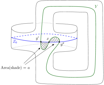
Figure 1. A plumbing of two $T^{*}S^{1}$ where $Z_{0}$ and $Y$ are two embedded Lagrangians.

In what follows we will view $Z_{0}$ and $Y$ as marked Lagrangians and denote by $\bar{Z}_{0}$ and $\bar{Y}$ their underlying Lagrangians. We will shortly be a bit more specific regarding the marking of $Z_{0}$ and $Y$, namely the grading and the choice of primitives for the Liouville form on these Lagrangians. Let $\bar{\mathcal{X}}$ be any collection of exact Lagrangians in $X$ that contains $\bar{Z}_{0}$ and $\bar{Y}$ and such that $\bar{\mathcal{X}}$ satisfies the conditions from §2.6.2. For the family $\mathcal{X}$ we take, as before, the Lagrangians in $\bar{\mathcal{X}}$ together with all their possible markings (i.e. we endow each Lagrangian $\bar{L}\in\bar{\mathcal{X}}$ with all possible primitives of $\lambda|_{\bar{L}}$ and all possible grading).

Recall from §2.6 that in our realization of the Fukaya category we take Floer data with $0$ Hamiltonians for pairs of Lagrangians that intersect transversely. This applies in particular to $Z_{0}$ and $Y$, hence the Floer complex $CF_{*}(Z_{0},Y)$ is generated by the intersection points between $Z_{0}$ and $Y$, which are $y^{\prime},x,y^{\prime\prime}$.

We endow $Z_{0}$ and $Y$ with gradings such that:

$$|y^{\prime}|=|y^{\prime\prime}|=0,\text{ and }|x|=1,$$

where $|\cdot|$ stands for homological grading. It follows that the Floer complex (with $\mathbb{Z}_{2}$-coefficients) has the following form:

$$CF_{0}(Z_{0},Y)=\mathbb{Z}_{2}y^{\prime}\oplus\mathbb{Z}_{2}y^{\prime\prime},\qquad dy^{\prime}=dy^{\prime\prime}=0,$$ (132)

$$CF_{1}(Z_{0},Y)=\mathbb{Z}_{2}x, dx=y^{\prime}+y^{\prime\prime}.$$

We now turn to the action filtration on the Floer complex. We choose primitives for $\lambda|_{\bar{Z}_{0}}$ and $\lambda|_{\bar{Y}}$ such that the actions of the intersection points of $Z_{0}\cap Y$ are given by:

$$\mathcal{A}(y^{\prime})=\mathcal{A}(y^{\prime\prime})=0,\quad\mathcal{A}(x)=a,$$ (133)

where $a$ is the area depicted in Figure 1.

It follows that the persistence Floer homology $HF_{*}(Z_{0},Y)$ is concentrated in degree $0$ and moreover the persistence module $HF_{0}(Z_{0},Y)$ has the following barcode:

$$\mathcal{B}_{HF_{0}(Z_{0},Y))}=\bigl{\{}[0,a),[0,\infty)\bigr{\}}.$$ (134)

We denote the resulting filtered Fukaya category by $\mathcal{F}uk(\mathcal{X};\mathscr{P})$ - see §2.6.2.

Consider a surgery of $Z_{0}\cup Y$ at $y^{\prime}$, so that the outcome Lagrangian is represented by the immersed Lagrangian $S_{\epsilon}$ (depicted in red) in Figure 2, with two self-intersection points $x$, $y^{\prime\prime}$. Here $\epsilon$ is the area of the surgery handle used in the surgery at $y^{\prime}$ (see [26, 22, 4] for a detailed description of surgery.) Note that $S_{\epsilon}$ is an exact immersed Lagrangian (this is always the case when we perform surgery of two exact Lagrangians at a single point). Since the choices of the primitives of $\lambda|_{\bar{Z}_{0}}$ and $\lambda|_{Y}$ coincide at $y^{\prime}$ (recall that $\mathcal{A}(y^{\prime})=0$) we can endow $S_{\epsilon}$ with a primitive induced by those of $Z_{0}$ and $Y$ (more precisely, one needs to parametrize $S_{\epsilon}$ by an immersion $j:\hat{S}\longrightarrow X$ with $j(\hat{S})=S$ such that $j^{*}\lambda$ is exact and define the primitive of the latter $1$-form on $\hat{S}$). We also perturb slightly this $S_{\epsilon}$ by a a small Hamiltonian perturbation of Hofer norm at most $\epsilon^{\prime}$ thus getting $S=S_{\epsilon,\epsilon^{\prime}}$ that intersects transversely all the elements in $\bar{\mathcal{X}}$.

It can easily be seen that $S$ is unobstructed (in the sense that it carries no pseudo-holomorphic teardrops (see also [6])). Therefore, $S$ gives rise to a filtered $A_{\infty}$-module over $\mathcal{F}uk(\mathcal{X})$, which we denote by $\mathscr{S}$. The existence of this module requires in fact elements of the theory of immersed Fukaya category mentioned in Remark 8.2.1 (ii), however only the most elementary part of this theory is needed here. In essence, because $S$ is unobstructed we can include $S$ in a larger family $\mathcal{X}^{\prime}$ that contains $\mathcal{X}$ and $S$. We may still define a Fukaya filtered category associated to $\mathcal{X}^{\prime}$, $\mathcal{F}uk(\mathcal{X}^{\prime};\mathscr{P}^{\prime})$. The immersed Lagrangian $S$ now gives a (filtered) Yoneda module $\mathcal{Y}(S)$ over $\mathcal{F}uk(\mathcal{X}^{\prime};\mathscr{P}^{\prime})$. The perturbation data $\mathscr{P}^{\prime}$ can be picked to be admissible also for the set $\mathcal{X}$ and there is an embedding $\mathcal{F}uk(\mathcal{X};\mathscr{P}^{\prime})\to\mathcal{F}uk(\mathcal{X}^{\prime};\mathscr{P}^{\prime})$ such that $\mathcal{Y}(S)$ pulls back to a module over $\mathcal{F}uk(\mathcal{X};\mathscr{P}^{\prime})$. Finally, using that $\mathcal{F}uk(\mathcal{X})$ is independent of the perturbation data up to filtered quasi-equivalence, we can pull-back this module to the module $\mathscr{S}$ over $\mathcal{F}uk(\mathcal{X};\mathscr{P})$. The details of this process appear in [10, Chapter 3, Theorem 3.12], but only in the case when $S$ is embedded. The modifications needed for our $S$ here are easy to implement as in [6] (where is covered the construction of non-filtered, Fukaya type categories with immersed objects in much larger generality), and noting that the construction there of the Floer complexes of the type $CF(S,S)$, $CF(S,X)$, $CF(X,S)$ (for $X\in\mathcal{X}$) produces filtered structures, and similarly for the higher $A_{\infty}$-operations.

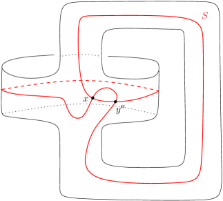
Figure 2. An immersed Lagrangian from a surgery at $y^{\prime}$.

Next, consider the twisted complex (over $\mathcal{F}uk(\mathcal{X})$) defined as the mapping cone

$$\mathscr{C}:=\text{Cone}(Z_{0}\xrightarrow{\;y^{\prime}\;}Y)$$ (135)

of the morphism $y^{\prime}\in\hom_{\mathcal{F}uk(\mathcal{X})}(Z_{0},Y)=CF_{0}(Z_{0},Y)$. (Recall that $y^{\prime}$ is a cycle). Since $y^{\prime}$ has filtration level $0$ and both $Z_{0}$, $Y$ are filtered twisted complexes, $\mathscr{C}$ can be endowed with the structure of a filtered twisted complex $\in\mathcal{C}^{\prime}\mathcal{F}uk(\mathcal{X})\subset\mathcal{C}\mathcal{F}uk(\mathcal{X})$ in the standard way.

We claim that $\mathscr{S}\in\mathcal{C}\mathcal{F}uk(\mathcal{X})$ and that there exists an $r$-isomorphism

$$\phi:\mathscr{C}\to\mathscr{S}$$

such that $r=r(\epsilon,\epsilon^{\prime})$ tends to $0$ when both $\epsilon$ and $\epsilon^{\prime}$ go to $0$.

To prove this we compare $\mathcal{Y}(S)$ and $\mathscr{C}$ over the category $\mathcal{F}uk(\mathcal{X}^{\prime};\mathcal{P}^{\prime})$, and we notice the existence of an $r$-isomorphism

$$\bar{\phi}:\mathscr{C}\to\mathcal{Y}(S)$$

of the form $\mu_{2}(\alpha,-)$ for an appropriate intersection point $\alpha$ between $S$ and $Z_{0}\cup Y$. To see this we can interpret $\mathscr{C}=\mathcal{Y}(S^{\prime})$ where $S^{\prime}$ is a marked immersed Lagrangian, in the sense discussed in §8.2, with obvious primitive and grading, and with a marked point $I_{\mathscr{C}}=\{y^{\prime}\}$. At this point it is also useful to use the $\epsilon^{\prime}$-small Hamiltonian perturbation to be a bit special, in essence associated to a Morse function with two critical points on $\hat{S}$ and in this case $\alpha$ is the intersection point between $S_{\epsilon,\epsilon^{\prime}}$ and $S^{\prime}$ that corresponds to the maximum of this function. By pulling back $\bar{\phi}$ over $\mathcal{F}uk(\mathcal{X})$ we get $\phi$.

We now pass to calculations in the $K$-group $K(\mathcal{C}\mathcal{F}uk(\mathcal{X}))$. We have:

$$[\mathscr{C}]=-[Z_{0}]+[Y]\in K(\mathcal{C}\mathcal{F}uk(\mathcal{X})).$$ (136)

Next we compute the pairing $\kappa([\mathscr{C}],\mathscr{C}])$. By linearity, and by Theorem 8.1.2 we obtain:

$$\kappa([\mathscr{C}],[\mathscr{C}]) =\kappa([Y],[Y])+\kappa([Z_{0}],[Z_{0}])-\kappa([Y],[Z_{0}]))-\kappa([Z_{0}],[Y])$$ (137)

$$=-\chi(Y)-\chi(Z_{0})-\lambda_{HF_{*}(Z_{0},Y)}(t)+\lambda_{HF_{*}(Z_{0},Y)}(t^{-1})$$

$$=0+0-(1-t^{a}+1)+(1-t^{-a}+1)$$

$$=-t^{-a}+t^{a},$$

where the third equality comes from the barcode data (134) and the identities in Theorem 8.1.2.

Since $\kappa([\mathscr{C}],[\mathscr{C}])$ is not a constant, by Corollary 8.1.2, the class $[\mathscr{S}]=[\mathscr{C}]\in K(\mathcal{C}\mathcal{F}uk(\mathcal{X}))$ cannot be represented by any Lagrangian in $\mathcal{X}$ .

Further, we now want apply Theorem 8.1.4. First , the data before provide a reduced resolution $D$ of weight $r$ of $\mathscr{S}$ with linearization $\ell(D)=(T^{-1}Y,Z_{0})$.

Clearly, $[D]=-[\mathscr{C}]$ so $\mathrm{gap}(\kappa([D],[D]))=a$. Obviously $n_{D}=2$. It is also immediate to calculate $b_{\max}^{\#}(\{T^{-1}Y,Z_{0}\})=2$. We fix $\mathcal{F}=\{T^{-1}Y,Z_{0}\}$. Thus, we obtain

$$\mathscr{R}^{\mathcal{F}}(\mathscr{S})\leq\frac{8r}{a}~{}.~{}$$

Theorem 8.1.4 implies that if $r=r(\epsilon,\epsilon^{\prime})\leq\frac{a}{16}$, then $\mathscr{C}$ can not represent an embedded Lagrangian (in the sense that it is not the Yoneda module of an element in $\mathcal{X}$). Moreover, this result is independent of the set $\mathcal{X}$ as long as $\mathcal{X}$ contains $Z_{0},Y$.

Another way to apply Theorem 8.1.4 is to deduce by an argument very similar to the above that, assuming that both $\epsilon$ and $\epsilon^{\prime}$ are very small, then the Hofer norm of a Hamiltonian homotopy needed to deform $S$ into an embedding is at least $\frac{a}{16}$.

Remark 8.3.1.

As noted in relation to the constant $4$ in Theorem 8.1.4, the constant $16$ here is not optimal. In essence, the argument we discussed is very general but it produces constants that can be easily improved in our example. In this example it is possible to use a Hamiltonian homotopy of energy $a$ to deform $S$ into an embedding and it is likely that this is sharp.

References

- [1] G. Alston and E. Bao. Immersed Lagrangian Floer cohomology via pearly trajectories. Preprint (2019). Can be found at https://arxiv.org/abs/1907.03072.
- [2] U. Bauer and M. Lesnick. Induced matchings and the algebraic stability of persistence barcodes. J. Comput. Geom., 6(2):162–191, 2015.
- [3] N. Berkouk. On the (non-)stability of the sheaf-function correspondence. Preprint (2022). Can be found at https://arxiv.org/pdf/2207.06335.
- [4] P. Biran and O. Cornea. Lagrangian cobordism. I. J. Amer. Math. Soc., 26(2):295–340, 2013.
- [5] P. Biran and O. Cornea. Lagrangian cobordism and Fukaya categories. Geom. Funct. Anal., 24(6):1731–1830, 2014.
- [6] P. Biran and O. Cornea. A Lagrangian pictionary. Kyoto J. Math., 61(2):399–493, 2021.
- [7] P. Biran, O. Cornea, and E. Shelukhin. Lagrangian shadows and triangulated categories. Astérisque, (426):128, 2021.
- [8] P. Biran, O. Cornea, and J. Zhang. Filtered derived categories. In progress.
- [9] P. Biran, O. Cornea, and J. Zhang. Triangulation and persistence: Algebra 101. Preprint (2021). Can be found at https://arxiv.org/abs/2104.12258.
- [10] P. Biran, O. Cornea, and J. Zhang. Triangulation, Persistence, and Fukaya categories. Preprint (2023). Can be found at https://arxiv.org/abs/2304.01785.
- [11] O. Bobrowski and M. S. Borman. Euler integration of Gaussian random fields and persistent homology. J. Topol. Anal., 4(1):49–70, 2012.
- [12] M. Botnan, S. Oppermann, and S. Oudot. Signed barcodes for multi-parameter persistence via rank decompositions. In 38th International Symposium on Computational Geometry (SoCG 2022), volume 224 of LIPIcs. Leibniz Int. Proc. Inform., pages Paper No. 19, 18. Schloss Dagstuhl. Leibniz-Zent. Inform., Wadern, 2022.
- [13] L. Buhovsky, J. Payette, I. Polterovich, L. Polterovich, E. Shelukhin, and V. Stojisavljević. Coarse nodal count and topological persistence. Preprint (2022). Can be found at https://arxiv.org/pdf/2206.06347.
- [14] E. Campling. Fukaya categories of Lagrangian cobordisms and duality. Preprint (2019). Can be found at https://arxiv.org/abs/1902.00930.
- [15] K. Costello. Topological conformal field theories and Calabi-Yau categories. Adv. Math., 210(1):165–214, 2007.
- [16] S. Ganatra. Symplectic Cohomology and Duality for the Wrapped Fukaya Category. ProQuest LLC, Ann Arbor, MI, 2012. Thesis (Ph.D.)–Massachusetts Institute of Technology.
- [17] D. Govc and R. Hepworth. Persistent magnitude. J. Pure Appl. Algebra, 225(3):Paper No. 106517, 40, 2021.
- [18] M. Kashiwara. Index theorem for constructible sheaves. Number 130, pages 193–209. 1985. Differential systems and singularities (Luminy, 1983).
- [19] M. Kashiwara and P. Schapira. Categories and sheaves, volume 332 of Grundlehren der mathematischen Wissenschaften [Fundamental Principles of Mathematical Sciences]. Springer-Verlag, Berlin, 2006.
- [20] M. Kashiwara and P. Schapira. Persistent homology and microlocal sheaf theory. J. Appl. Comput. Topol., 2(1-2):83–113, 2018.
- [21] M. Kontsevich and Y. Soibelman. Notes on -algebras, -categories and non-commutative geometry. In Homological mirror symmetry, volume 757 of Lecture Notes in Phys., pages 153–219. Springer, Berlin, 2009.
- [22] F. Lalonde and J.-C. Sikorav. Sous-variétés lagrangiennes et lagrangiennes exactes des fibrés cotangents. Comment. Math. Helv., 66(1):18–33, 1991.
- [23] S. Mac Lane. Categories for the working mathematician, volume 5 of Graduate Texts in Mathematics. Springer-Verlag, New York, second edition, 1998.
- [24] V. Lebovici. Hybrid transforms of constructible functions. Preprint (2021). Can be found at https://arxiv.org/pdf/2111.07829.
- [25] P. May. The axioms for triangulated categories. Can be found at http://www.math.uchicago.edu/~may/MISC/Triangulate.pdf.
- [26] L. Polterovich. The surgery of Lagrange submanifolds. Geom. Funct. Anal., 1(2):198–210, 1991.
- [27] L. Polterovich, D. Rosen, K. Samvelyan, and J. Zhang. Topological persistence in geometry and analysis, volume 74 of University Lecture Series. AMS, Providence, RI, 2020.
- [28] L. Polterovich, E. Shelukhin, and V. Stojisavljević. Persistence modules with operators in Morse and Floer theory. Mosc. Math. J., 17(4):757–786, 2017.
- [29] The Stacks project. 15.58 Derived tensor product. Can be found at https://stacks.math.columbia.edu/tag/06XY.
- [30] P. Schapira. Operations on constructible functions. J. Pure Appl. Algebra, 72(1):83–93, 1991.
- [31] P. Seidel. Fukaya categories and Picard-Lefschetz theory. Zurich Lectures in Advanced Mathematics. European Mathematical Society (EMS), Zürich, 2008.
- [32] D. Tamarkin. Microlocal condition for non-displaceability, volume 269 of Springer Proc. Math. Stat., pages 99–223. Springer, Cham, 2018.
- [33] M. Usher. Abstract interlevel persistence for Morse-Novikov and Floer theory. Preprint (2023). Can be found at https://arxiv.org/pdf/2302.14342.pdf.
- [34] M. Usher and J. Zhang. Persistent homology and Floer-Novikov theory. Geom. Topol., 20(6):3333–3430, 2016.
- [35] J. Zhang. -cyclic persistent homology and Hofer distance. J. Symplectic Geom., 17(3):857–927, 2019.
- [36] J. Zhang. Quantitative Tamarkin Theory. CRM Short Courses; Virtual Series on Symplectic Geometry. Springer International Publishing, 2020.