The spectrum of the Poincaré operator in an ellipsoid

Abstract

We study the spectrum of the Poincaré operator in triaxial ellipsoids subject to a constant rotation. As explained in the paper, this mathematical problem is interesting for many physical applications It is known that the spectrum of this bounded self-adjoint operator is pure point with polynomial eigenvectors. We give two new proofs of this result. Moreover, we describe the large-degree asymptotics of the restriction of that operator to polynomial vector fields of fixed degrees. The main tool is the microlocal analysis using the partial differential equation satisfied by the orthogonal polynomials in ellipsoids. This work also contains numerical calculations of these spectra, showing a very good agreement with the mathematical results.

1 Introduction

Large-scale flows in natural objects (e.g. planetary liquid cores or stars) are often subject to global rotation. A striking feature of such rotating flows is the ubiquitous presence of inertial waves (or modes in some geometries). These wave motions, which exist even without density effects for incompressible flows, are sustained by the Coriolis force [Kel80]. If the rotating fluid has a non-zero and spatially uniform vorticity $\vec{\Omega}\in{\mathbb{R}}^{3}$ (we define $\omega:=\|\vec{\Omega}\|$), these motions are in the simplest case small-amplitude perturbations governed by the linearized rotating Euler equation for all $t\in{\mathbb{R}}$ and the incompressible condition

$$u_{t}+\vec{\Omega}\wedge u=-\nabla p,\quad{\rm div}(u)=0,$$ (1a–b)

where the vector $u$ is the fluid velocity and the scalar $p$ is the pressure. Inertial modes can be excited by various mechanisms in natural objects, such as orbital (mechanical) forcings [RV10, NC13], surface viscous effects [AT69, CVS⁺21], or turbulent convection [Zha94, Lin21]. For instance, forced inertial modes might have been recently detected in the Sun [TGBR22]. Moreover, inertial modes are often key in the dynamics of rapidly rotating fluids. Nonlinear couplings of inertial modes can indeed sustain flow instabilities [Ker02, VCN15, VC23], turbulence [GFLBA17, LRFLB19] and, possibly, planetary (or stellar) magnetic fields through dynamo action [RFLB18, VCSH18].

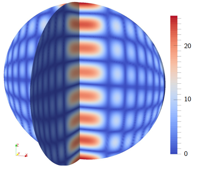
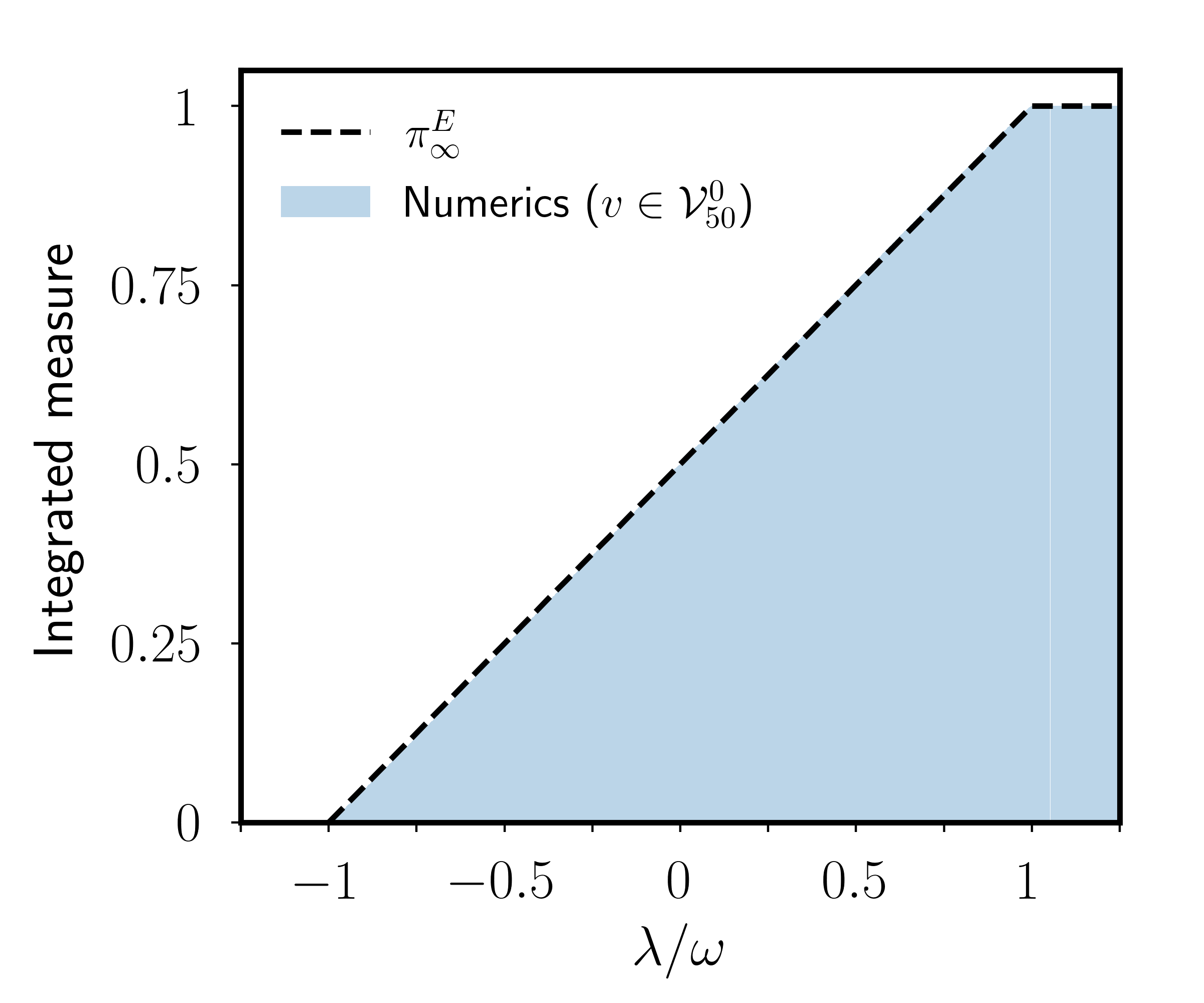
(a)	(b)

Figure 1: (a) Velocity magnitude $||v||$ of an inertial mode with angular frequency $\lambda\simeq 0.5412$ in the ellipsoid $A_{1}=A_{2}=1$ and $A_{3}\simeq 1.179$, rotating at the angular velocity $\vec{\Omega}=(0,0,1)$. (b) Integrated probability measure of all the eigenvalues for $v\in{\cal V}_{50}^{0}$ in the round ball [VSC20], which converges towards a uniform distribution.

Owing to their considerable importance for planetary or astrophysical applications, inertial modes (and their related flows) are often studied in ellipsoidal geometries [LBCLG15]. Indeed, rapidly rotating fluid masses are usually ellipsoidal at the leading order [Cha69] (because of centrifugal forces and, possibly, tidal interactions due to orbital partners). Let us give some definitions. For $A_{1},A_{2},A_{3}>~{}0$, we introduce the ellipsoid

$$E=\{x=(x_{1},x_{2},x_{3})\in{\mathbb{R}}^{3}|A_{1}x_{1}^{2}+A_{2}x_{2}^{2}+A_{3}x_{3}^{2}\leq 1\}.$$ (2)

We equip ${\mathbb{R}}^{3}$ with the canonical Euclidean structure and the canonical orientation. We denote by ${\cal V}$ the Hilbert space of vector fields in $E$ whose coefficients are in $L^{2}(E,|dx|)$, where $|dx|$ is the Lebesgue measure, and by ${\cal V}^{0}$ the closed subspace orthogonal to the vector fields that are gradients of smooth functions. A smooth element in ${\cal V}^{0}$ is divergenceless and tangent to the boundary (see chapter 3 in [Gal11]). Inertial modes are periodic solutions $u=e^{i\lambda t}v$ of equation (1), where the complex-valued eigenvector $v\in{\cal V}^{0}$ is given by

$$i\lambda v+\vec{\Omega}\wedge v=-\nabla p,\quad{\rm div}(v)=0,$$ (3a–b)

together with the no-penetration condition $\left.\langle v,\vec{n}\rangle\right|_{\partial E}=0$ on the ellipsoidal boundary $\partial E$ (where $\vec{n}$ is the unit normal vector to $\partial E$). An example of a large-scale inertial mode in an axisymmetric ellipsoid is shown in figure 1(a). Even in this simple physical configuration, solving the inertial mode problem is very challenging from a mathematical viewpoint. This is more clearly evidenced by considering the equation for the pressure (called the Poincaré equation after Cartan [Car22] who revisited Poincaré’s paper [Poi85])

$$\lambda^{2}\Delta p=(\vec{\Omega}\cdot\nabla)^{2}p,\quad\langle\nabla p,\vec{n}\rangle|_{\partial E}=\langle\vec{n},v\wedge\vec{\Omega}\rangle|_{\partial E}.$$ (4a–b)

The Poincaré equation is hyperbolic for $|\lambda|<\omega$, but, because of the boundary condition, the inertial-mode problem is an ill-posed Cauchy problem [RGV00]. Explicit solutions in ${\cal V}^{0}$ have been found in spheroids with $A_{1}=A_{2}$ and $\vec{\Omega}=(0,0,1)$ since the pioneering work of Bryan [Bry89], which admit exact Cartesian polynomial expressions [Kud66, ZL17]. Low-degree polynomial solutions in ${\cal V}^{0}$ have also been found in triaxial ellipsoids with $A_{1}\neq A_{2}\neq A_{3}$[Van14], but there are no explicit solutions for the higher-degree modes. Actually, the inertial-mode spectrum is pure point in ellipsoids and the polynomial eigenvectors form a complete set [BR17, Ive17]. The latter result could open new lines of research in fluid dynamics [Gre68], but the inertial-mode spectrum is still not well understood.

In this paper, we aim to better understand the properties of the inertial-mode spectrum in ellipsoids. We first prove, using another mathematical route, that the inertial-mode spectrum is pure point with polynomial eigenvectors. The same result was initially proved in axisymmetric cases [Den59], and recently extended to triaxial geometries [BR17, Ive17]. Then, we present new mathematical results on the asymptotic behaviour of the pure point spectrum in triaxial ellipsoids, which are successfully validated against numerical computations.

2 Poincaré operator in ellipsoids

2.1 Some generalities

We denote by ${\cal P}_{n}$ the space of polynomial functions from ${\mathbb{R}}^{3}$ to ${\mathbb{C}}$ of degree less or equal to $n$, by ${\cal V}_{n}$ the space of vector fields in $E$ whose coefficients are in ${\cal P}_{n}$ and by ${\cal V}_{n}^{0}={\cal V}_{n}\cap{\cal V}^{0}$ the subspace of ${\cal V}_{n}$ whose elements are the vector fields that are divergenceless and tangent to the boundary $\partial E$.

If we denote by $\Pi$ the orthogonal projection from ${\cal V}$ onto ${\cal V}^{0}$, called the Leray projector, we get the Poincaré operator $P$, which is a bounded self-adjoint operator on ${\cal V}^{0}$ defined by

$$Pv=i\Pi\left(\vec{\Omega}\wedge\Pi v\right).$$ (5)

The spectrum of $P$ is the set of values of $\lambda$ for which there are non-zero solutions of equation (3). We have the following result in ellipsoids [BR17]

Theorem 2.1

The spaces ${\cal V}_{n}^{0}$ are invariant by $P$. The spectrum of $P$ is the interval $[-\omega,\omega]$ and is pure point. There is an orthonormal basis of ${\cal V}^{0}$ consisting of eigenvectors of $P$ that have polynomial coefficients.

Note that this result is interesting for (at least) two reasons. First, the fact that the spectrum is pure point shows that there is no attractors in the classical dynamics. Second, the fact that the eigenmodes are polynomial allows a good numerical calculus of the spectra.

Next, we introduce the spaces ${\cal W}_{n}=\left({\cal V}_{n-1}^{0}\right)^{\perp}\cap{\cal V}_{n}^{0}$ of dimension $d_{n}=n(n+2)$. It follows from Theorem 2.1 and from the self-adjointness of $P$ that the spaces ${\cal W}_{n}$ are invariant by $P$. Our main result is about the asymptotic repartition of the eigenvalues $\mu_{j}^{n}$, with $j\in[1,d_{n}]$, of the restriction of $P$ to the spaces ${\cal W}_{n}$. To this end, we define the probability measures $\pi_{n}$ by

$$\pi_{n}:=\frac{1}{d_{n}}\sum_{j=1}^{d_{n}}\delta(\mu_{j}^{n}),$$ (6)

and we have the following theorem.

Theorem 2.2

As $n\rightarrow\infty$, the measures $\pi_{n}$ converge weakly to a probability measure $\pi_{\infty}$ of support $[-\omega,\omega]$. It means that, for every continuous function $f:{\mathbb{R}}\rightarrow{\mathbb{R}}$, we have

$$\lim_{n\rightarrow\infty}\frac{1}{d_{n}}\sum_{j=1}^{d_{n}}f(\mu_{j}^{n})=\int_{\mathbb{R}}fd\pi_{\infty}.$$ (7)

Remark 2.1

A weaker result is obtained by looking not at a fixed degree $n$, but at the joint the repartition of the $\{\mu_{j}^{l}\}$ for $j\in[1,d_{l}]$ and $l\leq n$. The limits are the same. This is this last measure that is numerically computed below in §7.

Previous numerical computations suggest that the probability density is uniform in the round ball (see figure 1b), but the properties of the spectral measure have not been investigated in ellipsoids before our work. The recipe for the construction of $\pi_{\infty}$ will be given in Section 6.

The previous results could be a good sarting point for studying classical problems such as other spectral asymptotics, control theory. See more on that in Section 9.

2.2 First proof of Theorem 2.1

We give here a first simple proof of Theorem 2.1, which is quite close in spirit of previous proofs [BR17, Ive17] but without using dimension arguments. We first show that ${\cal V}_{n}={\cal V}_{n}^{0}\oplus\nabla{\cal P}_{n+1}$. It follows from the Green formula that both spaces are orthogonal. Let us look at the orthogonal space of $\nabla{\cal P}_{n+1}$ in ${\cal V}_{n}$. If $v=a\partial_{x_{1}}+b\partial_{x_{2}}+c\partial_{x_{3}}$ is in ${\cal V}_{n}$ and orthogonal to $\nabla{\cal P}_{n+1}$, we have for any polynomial $\phi\in{\cal P}_{n+1}$

$$\int_{E}\phi~{}{\rm div}(v)\,d{x_{1}}d{x_{2}}d{x_{3}}-\int_{\partial E}\phi\langle v|\vec{n}\rangle\,d\sigma=0,$$

where

$$\vec{n}=\left(A_{1}^{2}{x_{1}}^{2}+A_{2}^{2}{x_{2}}^{2}+A_{3}^{2}{x_{3}}^{2}\right)^{-\frac{1}{2}}\left(A_{1}{x_{1}}\partial_{x_{1}}+A_{2}{x_{2}}\partial_{x_{2}}+A_{3}{x_{3}}\partial_{x_{3}}\right)$$

is the unit normal vector to $\partial E$. By taking $\phi=(A_{1}{x_{1}}^{2}+A_{2}{x_{2}}^{2}+A_{3}{x_{3}}^{2}-1){\rm div}(v)\in{\cal P}_{n+1}$, we get

$$\int_{E}(A_{1}{x_{1}}^{2}+A_{2}{x_{2}}^{2}+A_{3}{x_{3}}^{2}-1){\rm div}(v)^{2}\,d{x_{1}}d{x_{2}}d{x_{3}}=0$$

such that ${\rm div}(v)=0$. Let us then take $\phi=aA_{1}{x_{1}}+bA_{2}{x_{2}}+cA_{3}{x_{3}}\in{\cal P}_{n+1}$, we get

$$\int_{\partial E}({x_{1}}aA_{1}+{x_{2}}bA_{2}+{x_{3}}cA_{3})^{2}\left(A_{1}^{2}{x_{1}}^{2}+A_{2}^{2}{x_{2}}^{2}+A_{3}^{2}{x_{3}}^{2}\right)^{-\frac{1}{2}}d\sigma=0$$

such that $v$ is tangent to $\partial E$. The spaces ${\cal V}_{n}$ are invariant by $\vec{\Omega}~{}\wedge$. It follows that the spaces ${\cal V}_{n}^{0}$ are invariant by the Poincaré operator $P=i\Pi\vec{\Omega}\wedge\Pi$.

We have to show that $\oplus_{n\in{\mathbb{N}}}{\cal V}_{n}^{0}$ is dense in ${\cal V}^{0}$ for the $L^{2}$ topology. By the Stone-Weierstraß  Theorem, $\oplus_{n\in{\mathbb{N}}}{\cal V}_{n}$ is dense in ${\cal V}$. The space $K:=\left(\oplus_{n\in{\mathbb{N}}}{\cal V}_{n}^{0}\right)\oplus\left(\oplus_{n\in{\mathbb{N}}}\nabla{\cal P}_{n+1}\right)$ is dense in ${\cal V}={\cal V}_{0}\oplus\nabla H^{1}$. The respective densities of each term in $K$ follows. Thus, we have an orthonormal basis of $L^{2}$ eigenmodes and the spectrum is pure point.

It remains to prove that the spectrum is the full interval. This follows from the methods of Theorem 2.1 in [CdVSR20]. $P$ is inside $E$ a pseudo-differential operator, and the computation of the principal symbol $p$ of $P$ (see Section 6) shows that the image of the eigenvalues of $p$ is the interval $[-\omega,\omega]$. On the other hand, we have $\|P\|\leq\omega$. Hence, the full spectrum is $[-\omega,\omega]$. This holds for any bounded smooth domain. For ellipsoids, this follows also in the context of the present paper from Theorem 2.2 and 7.1.

2.3 Further spectral properties

Proposition 2.1

The numbers $\pm\omega$ are not eigenvalues of $P$ in ellipsoids.

The above result was proved in [BR17, Ive17], but we give below an alternative proof for $-\omega$. We assume that $v\in{\cal V}_{0}$ satisfies $\Pi\Omega\wedge v=i\omega v$. Then, by virtue of the Pythagorean theorem, we have $\vec{\Omega}\wedge v\in{\cal V}_{0}$ and $\vec{\Omega}\wedge v=i\omega v$. It follows that $v_{3}=0$ and $v_{1}=iv_{2}$. Then, using ${\rm div}(v)=0$, we see that $v_{1}$ is harmonic in $(x_{1},x_{2})$. Moreover, $(n_{1}-in_{2})v_{1}=0$ on $\partial E$ implies $v_{1}=0$ on $\partial E$. To finish, observe that on each level set $z=c$, $v_{1}$ is harmonic and vanishes on the boundary. So, we have $v_{1}=iv_{2}=0$ everywhere. Actually, the previous argument is valid for any smooth bounded domain in ${\mathbb{R}}^{3}$.

The subset of geostrophic modes, which are invariant along the rotation axis, often plays an important role in the dynamics of rapidly rotating flows [Gre68]. A vector field $v\in{\cal V}_{0}$ is geostrophic if $v$ is in the kernel of the Poincaré operator. We have the following result in ellipsoids (initially proved in [Ive17]). Without loss of generality, we can assume that $\vec{\Omega}=(0,0,1)$ and

$$E=\{x\in{\mathbb{R}}^{3}|Ax_{1}^{2}+Bx_{2}^{2}+x_{3}^{2}+2Cx_{1}x_{3}+2Dx_{2}x_{3}\leq 1\}.$$

This equation for $E$ is more convenient in the study of geostrophic fields. We were using the scaling invariance and a rotation around the $x_{3}-$axis to make the coefficient of $x_{3}^{2}$ equal to $1$ and the coefficient of $x_{1}x_{2}$ vanish.

Proposition 2.2

There exists exactly one geostrophic field in ${\cal W}_{n}$ for $n$ odd and no geostrophic field in ${\cal W}_{n}$ for $n$ even.

Let us denote by $F$ the projection of $E$ onto the $(x_{1},x_{2})-$plane. For each $(x_{1},x_{2})$ in the interior of $F$, there exist two points $(x_{1},x_{2},x_{3}^{\pm}(x_{1},x_{2}))$ in $\partial E$. From $\vec{\Omega}\wedge v=-\nabla p$, we get that $v=(v_{1},v_{2},v_{3})$ satisfies

$$v_{1}=-\partial p/{\partial x_{2}},\quad v_{2}=\partial p/{\partial x_{1}},\quad\partial p/{\partial x_{3}}=0,$$

and the boundary condition

$$(Ax_{1}+Cx_{3}^{\pm})v_{1}+(Bx_{2}+Dx_{3}^{\pm})v_{2}+(x_{3}^{\pm}+Cx_{1}+Dx_{2})v_{3}=0.$$

From $\partial p/{\partial x_{3}}=0$, we get that $p$ is independent of $x_{3}$. From the expressions of $v_{1}$ and $v_{2}$ in terms of $p$, we get that they are independent of $x_{3}$ too. Using ${\rm div}v=0$ one gets that $v_{3}$ is also independent of $x_{3}$. So that the four functions $[v_{1},v_{2},v_{3},p]$ are independent of $x_{3}$; this is called the Taylor-Proudman theorem [Gre68]. Eliminating $v_{3}$ from the previous two equations and replacing $v_{1}$ and $v_{2}$ in terms of $p$, we get that $p$ satisfies a differential equation $Vp=0$ where the coefficients of $V$ are linear in $(x_{1},x_{2})$:

$$V=(CDx_{1}-(B-D^{2})x_{2})\partial_{x_{1}}+((A-C^{2})x_{1}-CDx_{2})\partial_{x_{2}}.$$

If we write $V=M(x)\partial_{x}$, we see that ${\rm Trace}(M)=0$. Moreover the determinant of $M$ is

$$\delta=AB-BC^{2}-AD^{2}$$

which is also the determinant of the quadratic form defining $E$, hence $\delta>0$. We can then find a basis of ${\mathbb{R}}^{2}$ where $V=a(u\partial_{v}-v\partial_{u})$ with $a\neq 0$. This implies easily that there is a unique (up to dilation) non-zero quadratic form $Q$ with $VQ=0$ and no linear forms $L$ with $VL=0$: $Q=u^{2}+v^{2}$. All polynomials $p$ are then clearly of the form $p=F(Q)$ with $F$ a polynomial.

3 Orthogonal polynomials, Weyl law and a conceptual proof of Theorem 2.1

3.1 Orthogonal polynomials in Euclidean balls

Let us denote by ${\cal E}_{n}$ the space of polynomials of degree $n$ that are orthogonal to all polynomials of degree $\leq n-1$ in $L^{2}(B,|dx|)$, where $B$ is the Euclidean ball of radius $1$ in ${\mathbb{R}}^{3}$. The following result due to Appell and Kampé de Fériet [AKdF26] is proved in Section 5.2 of [DX01]:

Theorem 3.1

The spaces ${\cal E}_{n}$ are the eigenspaces of the operator $L$, which is called here the Legendre operator, defined by

$$L=-\sum_{i=1}^{3}\partial^{2}_{i}+\sum_{i,j=1}^{3}\partial_{i}x_{i}x_{j}\partial_{j}+9/4$$

with eigenvalue $(n+3/2)^{2}$ of multiplicity $d_{n}^{1}={(n+1)(n+2)}/{2}$.

Remark 3.1

We can define an operator $L$ in any dimension by a similar formula. In dimension $1$, the Legendre polynomials are eigenfunctions of the operator $L=-\partial_{x}^{2}+\partial_{x}x^{2}\partial_{x}$. They are orthogonal polynomials on $L^{2}([-1,1],|dx|)$.

We give below a simple proof of Theorem 3.1. For each $n\in{\mathbb{N}}$, $L$ acts on the space ${\cal P}_{n}$ of polynomials of degree $\leq n$. This action of $L$ is triangular. If we decompose ${\cal P}_{n}$ into a direct sum of homogeneous polynomials

$${\cal P}_{n}=\oplus_{k=0}^{n}{\cal H}_{k},$$

where ${\cal H}_{k}$ is the space of polynomials homogeneous of degree $k$. We have

$$L\left(\sum_{l=0}^{k}h_{l}\right)=(k+3/2)^{2}h_{k}+r_{k}$$

with ${\rm degree}(r_{k})\leq k-2$. Hence, the eigenvalues of $L$ restricted to ${\cal P}_{n}$ are the numbers $(k+3/2)^{2},~{}k=0,\cdots,n,$ with eigenspaces ${\cal H}_{k}\oplus{\cal R}_{k}$ with ${\cal R}_{k}\subset{\cal H}_{k-2}$.

Let us show that $L$ is symmetric on $C^{2}(\bar{B})$ and hence on each ${\cal P}_{n}$. There is a cancellation of boundary terms coming from both parts of $L$. Let us rewrite

$$L=-\Delta-D^{\star}D,$$

with $D=r\frac{d}{dr}$ and where $D^{\star}$ is the formal adjoint of $D$. By virtue of the Green-Riemann formula, we have

$$\int_{B}(u\Delta v-v\Delta u)|dx|=\int_{\partial B}\left(u\frac{\partial v}{\partial n}-v\frac{\partial u}{\partial n}\right)|d\sigma|.$$

On the other hand, we have also

$$\int_{B}\left(uD^{\star}Dv-vD^{\star}Du\right)|dx|=-\int_{\partial B}\left(u\frac{\partial v}{\partial r}-v\frac{\partial u}{\partial r}\right)|d\sigma|.$$

Both boundary terms cancel out since ${\partial}/{\partial r}={\partial}/{\partial n}$ on $\partial B$.

It follows that the eigenspaces of $L$ are exactly given by the orthogonal polynomials. The operator $L$ with domain $\oplus_{n\in{\mathbb{N}}}{\cal E}_{n}$ is essentially self-adjoint. It will be useful in particular in Section 4 to keep the notation $L$ for the differential operator and to denote by $\hat{L}$ its closure. Note that, if $u$ belongs to the Sobolev space $H^{2}(B)$ and is compactly supported in $B$, then $u\in D(\hat{L})$. $\square$

3.2 Weyl law

The principal symbol of $L$, denoted by $\Lambda$, is given by

$$\Lambda(x,\xi)=\|\xi\|^{2}-\langle x|\xi\rangle^{2}.$$

We see that $L$ is elliptic in the interior of $B$, but not on the boundary $\partial B$. The characteristic manifold is the co-normal bundle to the boundary.

The pull back of $\Lambda$ onto the Euclidean sphere $S^{3}\subset{\mathbb{R}}^{3}_{x}\oplus{\mathbb{R}}_{z}$ by the orthogonal projection $(x,z)\rightarrow x$ is the dual metric of the standard metric on $S^{3}$ (see Appendix A). Hence the operator $L$ is very similar to the Laplacian on $S^{3}$ and the eigenfunctions similar to the spherical harmonics. However the pull-back to $S^{3}$ of the Lebesgue measure on $B$ vanishes on the equator and is not the canonical measure on $S^{3}$. In fact, by looking at orthonormal polynomials in the balls with respect to the measure $(1-r²)^{-\frac{1}{2}}|dx|$, one could make a similar analysis leading to the usual spherical harmonics, more precisely to the spherical harmonics which are even under the change $z\rightarrow-z$.

Let us look at the Weyl formula:

Theorem 3.2

The eigenvalues counting function $N(\lambda)$ of $L$ satisfies

$$N(\lambda)\underset{\lambda\rightarrow\infty}{\sim}\lambda^{3/2}/6,$$

where the notation $\sim$ means that the ratio goes to $1$ as $\lambda\rightarrow\infty$. This expression coincides with the phase space volume calculated with respect to the Liouville measure:

$$\frac{1}{(2\pi)^{3}}{\rm Vol}(\{(x,\xi)\in T^{\star}B|\Lambda(x,\xi)\leq\lambda\})=\lambda^{3/2}/6.$$

The Weyl formula can be easily derived from the explicit expression of the eigenvalues, which is

$$N(\lambda)=\sum_{n+3/2\leq\sqrt{\lambda}}\frac{(n+1)(n+2)}{2}.$$

On the other hand, the calculus of the phase space volume is a simple exercise. Theorem 3.2 will be useful later in order to control the boundary effects.

In the case of ellipsoids, we get similar results by replacing $L$ by $L_{E}$ given by

$$L_{E}=-\sum_{i=1}^{3}\frac{\partial_{i}^{2}}{A_{i}}+\sum_{i,j=1}^{3}\partial_{i}x_{i}x_{j}\partial_{j}+\frac{9}{4}.$$

This is proved by using the affine diffeomorphism $\Phi:B\rightarrow E$ defined by

$$\Phi(x_{1},x_{2},x_{3})=\left(\frac{x_{1}}{\sqrt{A_{1}}},\frac{x_{2}}{\sqrt{A_{2}}},\frac{x_{3}}{\sqrt{A_{3}}}\right),$$

and remarking that $\Phi$ transforms the Lebesgue measure into a multiple of the Lebesgue measure and of course polynomials of degree $n$ into polynomials of degree $n$. Note that $\Phi$ also transforms also divergenceless vector fields that are tangent to the boundary in $B$ to vector fields with the same properties in $E$.

3.3 A conceptual proof of Theorem 2.1

The Leray projector is the orthogonal projector on vector fields $L^{2}$-orthogonal to the space of gradient of smooth functions. The operator $\sum_{i=1}^{3}(1/A_{i})\,\partial_{i}^{2}$ and the dilation operator ${\cal L}$ preserves the latter space. ${\cal L}$ is called the dilation operator, because it is the infinitesimal generator of the group of homotheties. This is also the case for its adjoint ${\cal L}^{\star}=-{\cal L}-3$. The Legendre operator $L_{E}=-\sum_{i=1}^{3}(1/A_{i})\,\partial_{i}^{2}-{\cal L}^{\star}{\cal L}+9/4$ is self-adjoint and preserves the space of gradients. It implies that the Legendre operator $L_{E}$ commutes with $\Pi$. This holds formally for any domain, but ${L_{E}}$ is a well-defined symmetric operator only on ellipsoids. Note then that any operator with constant coefficients like $\vec{\Omega}\,\wedge$ commutes with $L_{E}$. Hence, the Poincaré operator commutes with $L_{E}$. This gives a proof of Theorem 2.1 using only the spectral theory of $L_{E}$.

4 The microlocal Weyl law

This is the most technical part of this paper. We use the pseudo-differential boundary operator  calculus of Boutet de Monvel on manifolds with boundary [BdM71] (see also [Gru08] and Appendix C), as well as the construction of a parametrix for the “wave equation” $u_{tt}+Lu=0$ using Fourier Integral Operators coming from [Hör68, DG75].

Let $d_{n}^{1}:=\rm dim({\cal E}_{n})=(n+1)(n+2)/2$. We have the following result:

Theorem 4.1

Let $A$ be a self-adjoint pseudo-differential boundary operator  of degree $0$ in $B$ of principal symbol $\sigma(A)$. Let us denote by $(\phi_{j}^{n}),~{}j=1,\cdots,d_{n}^{1},$ an orthonormal basis of ${\cal E}_{n}$. We have in the large $n$ limit

$$\lim_{n\rightarrow+\infty}\frac{1}{d_{n}^{1}}\sum_{j=1}^{d_{n}^{1}}\langle A\phi_{j}^{n}|{\phi_{j}^{n}}\rangle=\frac{6}{(2\pi)^{3}}\int_{\Lambda\leq 1}\sigma(A)|dxd\xi|.$$

Proof.– We use the method of the papers [CdV79, Wei77] which are inspired from Hörmander [Hör68] (see also [DG75], section 2). We have two main difficulties: the fact that we have to work with a manifold with boundary and the fact that $L$ is not elliptic at the boundary. For that we will make first an assumption on $A$ avoiding both difficulties and then make approximations of $A$.

4.1 The case where $A$ is a “nice” pseudo-differential boundary operator

If $A$ is a pseudo-differential boundary operator, $WF^{\prime}(A)$ is the conic support of the full symbol of the pseudo-differential operator  part of $A$. The conical set $Z$ is the set of points in the phase space $T^{\star}B\setminus 0$ such that the Hamiltonian flow of $\Lambda$ hits $\partial B$ at a characteristic point, namely a point in $N^{\star}\partial B$ (see Appendix A). We have

$$Z=\{(x,\xi)\in T^{\star}B\setminus 0|\xi=sx{~{}\rm for~{}some~{}}s\in{\mathbb{R}}\}.$$

In the following, it will be important to make a difference between $L$ as a differential operator acting in ${\mathbb{R}}^{3}$, and the self-adjoint operator on $L^{2}(B)$ denoted by $\hat{L}$.

Definition 4.1

A pseudo-differential boundary operator $A$ is nice if it satisfies

$$WF^{\prime}(A)\cap\left(Z\cup\left(\partial B\times{\mathbb{R}}^{3}\setminus 0\right)\right)=\emptyset.$$

Recall that, if $K:{\mathbb{R}}\rightarrow L({\cal H})$, we can sometimes define the distributional trace as the Schwartz distribution defined by

$$\langle{\rm Trace}K|\phi\rangle={\rm Trace}\int_{\mathbb{R}}K(t)\phi(t)dt,$$

where $\phi$ is a test function and the trace in the right-hand side is the usual trace of trace class operator. The singularities of the distributional trace

$$Z:t\rightarrow Z(t):={\rm Trace}\left(e^{-it\sqrt{\hat{L}}}A\right)=\sum_{n=0}^{\infty}a_{n}e^{-it(n+3/2)},$$

with $a_{n}=\sum_{j=1}^{d_{n}^{1}}\langle A\phi_{j}^{n}|\phi_{j}^{n}\rangle$, determine the asymptotics of the sequence $(a_{n})_{n\in{\mathbb{N}}}$ (see Lemma B.1).

We define $\sqrt{\hat{L}}$ using the functional calculus for positive self-adjoint operators. However, $L$ is not elliptic and $\sqrt{\hat{L}}$ is not a pseudo-differential boundary operator  at characteristic points. It is more convenient to start from $\cos\left(t\sqrt{\hat{L}}\right)$. The solution of the wave equation

$$\square u:=u_{tt}+\hat{L}u=0,~{}u(0)=u_{0},~{}u_{t}(0)=0$$

is $u(t)=\cos\left(t\sqrt{\hat{L}}\right)u_{0}$. If

$$C:t\rightarrow C(t):={\rm Trace}\left(\cos\left(t\sqrt{\hat{L}}\right)A\right),$$

we have

$$Z=2HC$$

where $H$ is the “Hilbert” projector defined by

$${\cal F}(Hf)(\tau)={\rm Heaviside}(-\tau){\cal F}(f)(\tau)$$

with ${\cal F}(f)(\tau)=\int_{\mathbb{R}}e^{-it\tau}f(t)$ the Fourier transform of a function $f$. Hence, the singularities of $Z$ can be deduced from those of $C$.

Let us denote by ${\cal E}:=\{(x,\xi)\in T^{\star}{\mathbb{R}}^{3}|\Lambda(x,\xi)>0\}$ (the “elliptic” domain), by $\phi_{t},~{}t\in{\mathbb{R}},$ the Hamiltonian flow of $\sqrt{\Lambda}$ and by

$${\cal L}_{\pm}:=\{(t,\tau;x,\xi;y,\eta)|(x,\xi)=\phi_{\pm t}(y,\eta)|\tau\pm\sqrt{\Lambda}(x,\xi)=0,~{}(y,\eta)\in{\cal E}\}$$

the Lagrangian submanifolds of $T^{\star}({\mathbb{R}}_{t}\times{\mathbb{R}}^{3}_{x}\times{\mathbb{R}}^{3}_{y})$ associated to the flow $\phi_{t}$.

Lemma 4.1

If $A$ is a nice pseudo-differential operator  of degree $0$ (see the definition 4.1), the Schwartz kernel of $\cos\left(t\sqrt{\hat{L}}\right)A$ is the restriction to ${\mathbb{R}}\times B\times B$ of a Fourier Integral Operator  of degree $0$ associated to the union of the Lagrangian manifolds ${\cal L}_{\pm}$ modulo an operator $R(t)$ whose trace is a smooth function of $t$.

Proof.– In ${\mathbb{R}}^{3}$, the equation

$$\square u=0,~{}u(0)=Au_{0},~{}\dot{u}(0)=0$$

admits a Fourier Integral Operator  parametrix $U(t)$ as in [DG75], section 1: this is possible because ${\cal L}_{\pm}\subset T^{\star}{\mathbb{R}}\times{\cal E}\times{\cal E}$. It means that $\square U(t)$ has a smooth kernel on ${\mathbb{R}}\times{\mathbb{R}}^{3}\times{\mathbb{R}}^{3}$ and that $U(0)={\rm A}$ and $U_{t}(0)=0$ modulo operators with smooth kernels. We define then, for $u_{0}\in L^{2}(B)$, $V(t)u_{0}=\left(U(t)u_{0}\right)_{|{{B}}}$. The operator $V(t)$ is a parametrix for $\cos\left(t\sqrt{\hat{L}}\right)A$: it means that, if $u_{0}\in D(\hat{L})$, $V(t)u_{0}\in D(\hat{L})$, $S:=\square V(t)$ has a smooth kernel on ${\mathbb{R}}\times B\times B$ and that $U(0)={\rm A}$ and $U_{t}(0)=0$ modulo operators with smooth kernels.

If $u_{0}\in D(\hat{L})$, then $Au_{0}$ belongs to the Sobolev space $H^{2}(B)$. It follows from the continuity properties of FIO’s that, for all $t\in{\mathbb{R}}$, $V(t)u_{0}$ is also in $H^{2}(B)$ and hence in the domain of $\hat{L}$. The other properties follow from the properties of $U(t)$.

If $\cos\left(t\sqrt{\hat{L}}\right)A=V(t)+R(t)$, we have $\square R(t)=-S(t)$ and $R(0),~{}{R}_{t}(0)$ are smoothing. We get

$$R(t)=e^{it\sqrt{\hat{L}}}R_{1}+e^{-it\sqrt{\hat{L}}}R_{2}+\int_{0}^{t}e^{i(t-s)\sqrt{\hat{L}}}R_{3}(s)ds+\int_{0}^{t}e^{-i(t-s)\sqrt{\hat{L}}}R_{4}(s)ds,$$

where the $R_{j}$’s have smooth Schwartz kernels. It follows that they belong to the domains of all powers of $\hat{L}$, hence using the fact that, for all $N\geq 2$, $e^{it\sqrt{\hat{L}}}\hat{L}^{-N}$ is trace class, we get the smoothness of $t\rightarrow{\rm Trace}(R(t))$. $\square$

The bicharacteristic flow lifts to the geodesic flow on $S^{3}$ which is simply periodic of period $2\pi$: the orbits starting outside $Z$ are projections of great circles of $S^{3}$, hence ellipses tangent to $\partial B$ (see Appendix A). This implies that there are no periodic orbits of period smaller than $2\pi$ in ${\cal L}_{\pm}$. Using the argument of [DG75], Corollary 1.2, we deduce from the calculi of wave-front sets that the distribution $C$ is only singular at the points $2\pi n$ with $n\in{\mathbb{Z}}$. The antiperiodic distribution $Z=2HC$ is also singular only at the points $2\pi n$ with $n\in{\mathbb{Z}}$.

The analysis of [Hör68, DG75] shows that the Fourier transform of $\rho Z$, with $\rho\in C_{o}^{\infty}(]-2\pi,2\pi[)$ with $\rho(0)=1$, is a symbol $\tau\rightarrow\sigma(\tau)$ of degree $2$ and principal part

$$\sigma_{2}(\tau)=\frac{6\tau^{2}}{(2\pi)^{3}}\int_{\Lambda\leq 1}\sigma(A)|dxd\xi|.$$

Theorem 4.1 in the case where $A$ is nice follows then from Lemma B.1.

4.2 The general case

Let us give some $\varepsilon>0$ and rewrite $A$ as $A=A_{\varepsilon}+R_{\varepsilon}$ in the following way. We choose a pseudo-differential boundary operator $Q_{\varepsilon}=\chi_{\varepsilon}+\eta_{\varepsilon}$ of degree $0$ so that, denoting by $d$ the Euclidean distances,

1. $\chi_{\varepsilon}:\bar{B}\rightarrow[0,1]$ is smooth, equal to $1$ if $d(x,\partial B)\leq\varepsilon/2$ and vanishes if $d(x,\partial B)\geq\varepsilon$.

2. $\eta_{\varepsilon}$ is a compactly supported pseudo-differential operator  in $B$ whose full symbol is $1$ in the cone $\{(x,\xi)|d((x,\xi),Z)\leq\varepsilon/2\|\xi\|{\rm~{}and~{}}d(x,\partial B)\geq\varepsilon/2\}$ and $0$ in the cone $\{(x,\xi)|d((x,\xi),Z)\geq\varepsilon\|\xi\|{\rm~{}and~{}}d(x,\partial B)\leq\varepsilon/4\}$.

Let us decompose $A$ by putting $R_{\varepsilon}=Q_{\varepsilon}^{\star}AQ_{\varepsilon}$, and see that $A-R_{\varepsilon}$ is nice. We have

$$A=P+G,$$

where $G$ is a Green operator (see Appendix C). We have then

$$A-R_{\varepsilon}=\left(P-Q_{\varepsilon}^{\star}PQ_{\varepsilon}\right)+\left(G-Q_{\varepsilon}^{\star}GQ_{\varepsilon}\right).$$

The first term $P-Q_{\varepsilon}^{\star}PQ_{\varepsilon}$ is nice. Then, we need to prove that $B:=G-Q_{\varepsilon}^{\star}GQ_{\varepsilon}$ is smoothing: $(1-Q_{\varepsilon}^{\star})G$ is smoothing, then it remains to prove that

$$B=Q_{\varepsilon}^{\star}G(1-Q_{\varepsilon})$$

is smoothing: this is true because $1-Q_{\varepsilon}$ is smoothing near $\partial B$.

We have to estimate $r_{n}(\varepsilon):=\sum_{j=1}^{d_{n}^{1}}\langle R_{\varepsilon}\phi_{j}^{n}|\phi_{j}^{n}\rangle$. For any $\phi\in L^{2}$, we have

$$|\langle R_{\varepsilon}\phi|\phi\rangle|\leq C\langle Q_{\varepsilon}^{\star}Q_{\varepsilon}\phi|\phi\rangle$$

with $C=\|A\|$. Moreover, we have

$$\sum_{j=1}^{d_{n}^{1}}\langle Q_{\varepsilon}^{\star}Q_{\varepsilon}\phi_{j}^{n}|\phi_{j}^{n}\rangle=d_{n}^{1}-\sum_{j=1}^{d_{n}^{1}}\langle({\rm Id}-Q_{\varepsilon}^{\star}Q_{\varepsilon})\phi_{j}^{n}|\phi_{j}^{n}\rangle.$$

The last term can be evaluated because ${\rm Id}-Q_{\varepsilon}^{\star}Q_{\varepsilon}$ is nice, and we get

$$\lim_{n\rightarrow\infty}\frac{1}{d_{n}^{1}}\sum_{j=1}^{d_{n}^{1}}\langle\left({\rm Id}-Q_{\varepsilon}^{\star}Q_{\varepsilon}\right)\phi_{j}^{n}|\phi_{j}^{n}\rangle=\frac{6}{(2\pi)^{3}}\int_{\Lambda\leq 1}(1-\sigma(Q_{\varepsilon})^{2})|dxd\xi|.$$

The integral $\int_{\Lambda\leq 1}\sigma(Q_{\varepsilon})^{2}|dxd\xi|$ tends to $0$ as $\varepsilon\rightarrow 0$. It follows that $\lim\limits_{n\rightarrow\infty}(1/d_{n}^{1})r_{n}(\varepsilon)\rightarrow 0$ as $\varepsilon\rightarrow 0$.

5 A scalar version of Theorem 2.2

We will prove the following theorem

Theorem 5.1

Let $A$ be a self-adjoint pseudo-differential boundary operatorof degree $0$ in the Euclidean ball $B$, which commutes with the operator $\hat{L}$ and of principal symbol $\sigma(A)$. Let us denote by $\mu_{j}^{n},~{}j=1,\cdots,d_{n}^{1},$ the eigenvalues of $A$ restricted to ${\cal E}_{n}$. Then, when $n\rightarrow\infty$, the probability measures

$$\pi_{\lambda}:=\frac{1}{d_{n}^{1}}\sum_{j=1}^{d_{n}^{1}}\delta\left(\mu_{j}^{n}\right)$$ (8)

converge weakly to a probability measure $\pi_{\infty}$ that is defined as follows. For any continuous function $f:{\mathbb{R}}\rightarrow{\mathbb{R}}$, we have

$$\int_{\mathbb{R}}fd\pi_{\infty}=\frac{6}{(2\pi)^{3}}\int_{\Lambda\leq 1}f(\sigma(A))|dxd\xi|.$$ (9)

We can apply Theorem 4.1 to the operators $A^{N}$ with $N\in{\mathbb{N}}$. This gives

$$\langle A^{N}\phi_{j}^{n}|\phi_{j}^{n}\rangle=\left(\mu_{j}^{n}\right)^{N}.$$

Then, we get the asymptotics for $f$ a polynomial function. The answer for a continuous function $f$ is given by uniform approximation of $f$ by polynomial functions.

6 The proof of Theorem 2.2

Lemma 6.1

The operator $\Pi$ is a pseudo-differential boundary operator  in $B$ belonging to the Boutet de Monvel calculus (see Appendix C). The operator valued symbol of $\Pi$ at the point $(x,\xi)\in T^{\star}B\setminus 0$ is the orthogonal projection on the hyperplane $\ker(\xi)$.

Proof.– We use the isomorphism between vector fields and 2-forms given by $V\rightarrow\iota(V)dx_{1}\wedge dx_{2}\wedge dx_{3}$ where $\iota$ is the inner product. The image of the divergenceless vector fields tangent to the boundary is the closed 2-forms $\alpha$ satisfying $j^{\star}(\alpha)=0$ where $j:\partial B\rightarrow{\mathbb{R}}^{3}$ is the embedding. The relative cohomology $H^{2}(B,\partial B)$ vanishes: by Poincaré duality $H^{2}(B,\partial B)$ is isomorphic to $H_{1}(B)$ which vanishes. This implies that the Hodge Laplacian on 2-forms with the relative boundary conditions is invertible and the inverse is a pseudo-differential boundary operator in $B$. The projector $\Pi$ is then given by $\Pi=dd^{\star}\Delta^{-1}$ which is clearly also a pseudo-differential boundary operator. The symbol can be easily computed: the symbol of the divergence is the linear form $\xi$ and hence the symbol of $\Pi$ is the orthogonal projection onto the hyperplane $\ker\xi$. $\square$.

The spectrum of $P$ is the union of the eigenvalues of $P$ on ${\cal V}_{0}$, the $\lambda_{j}^{n}$’s with $n\in{\mathbb{N}},~{}1\leq j\leq d_{n}$, and the eigenvalue $0$ with eigenspace ${\cal V}_{0}^{\perp}$. We can compute the principal symbol $\sigma({P})$ of the Poincaré operator using Lemma 6.1 and the composition rules of symbols. If we denote by $\phi\in[0,\pi]$ the angle between $\vec{\Omega}$ and $\xi$, the eigenvalues of $\sigma({P})(x,\xi)$ are $(0,\Lambda_{1}:=\omega\cos\phi,-\Lambda_{1})$. If $\vec{\Omega}=(0,0,\omega)$, this can be written

$$\left(0,\omega\frac{\xi_{3}}{\|\xi\|},-\omega\frac{\xi_{3}}{\|\xi\|}\right).$$

We see that these eigenvalues are simple if $\xi_{3}\neq 0$ where all eigenvalues vanish.

We will now prove Theorem 2.2. The measure $\pi_{\infty}^{E}$ is defined by

$$\int_{\mathbb{R}}fd\pi_{\infty}=\frac{6}{(2\pi)^{3}}\int_{\sigma(L_{E})\leq 1}f(\Lambda_{1})|dxd\xi|.$$

In other words, we have

$$\int_{-\infty}^{t}d\pi_{\infty}^{E}=\frac{6}{(2\pi)^{3}}{\rm Vol}\left(\{(x,\xi)\in E\times{\mathbb{R}}^{3}|\sigma(L_{E})(x,\xi)\leq 1{~{}\rm and~{}}\omega\xi_{3}\leq t\|\xi\|\}\right).$$ (10)

Recall the dimension involved in what follows: $d_{n}=3d_{n}^{1}-d_{n+1}^{1}=n(n+2)$ is the dimension of polynomial vector fields in ${\cal V}_{n}^{0}$ orthogonal to ${\cal V}_{n-1}$ The proof is a corollary of Theorem 5.1. When $f$ is a polynomial, we get

$${\rm Trace}\left(e^{-it\sqrt{\hat{L}}}f(\tilde{P})\right)=\sum_{n=0}^{\infty}e^{-it(n+3/2)}\sum_{j=1}^{3d_{n}^{1}}f(\mu_{j}^{n})$$

where the $\mu_{j}^{n},~{}j=1,\cdots,3d_{n}^{1},$ are the eigenvalues of ${P}$ restricted to $\oplus_{i=1}^{3}{\cal E}^{n}$. This set is the union the eigenvalues of the restriction to divergenceless vector fields which is of interest for us and the eigenvalue $0$ corresponding to gradient vector fields, namely $\ker\Pi$, of multiplicity $d_{n+1}^{1}$.

On the other hand, the symbol of the operator $e^{-it\sqrt{\hat{L}}}f(\tilde{P})$ is the symbol of the Fourier Integral Operator  $e^{-it\sqrt{\hat{L}}}$ multiplied by the symbol of $f(\tilde{P})$. Taking the trace, we obtain for the measure

$$\tilde{\pi}_{n}:=\frac{1}{3d_{n}^{1}}\left(d_{n+1}^{1}\delta(0)+\sum_{j=1}^{d_{n}}\delta(\mu_{j}^{n}))\right)$$

the limit

$$\int_{\mathbb{R}}fd\tilde{\pi}_{\infty}=\frac{f(0)}{3}+\frac{2}{(2\pi)^{3}}\int_{\sigma(L_{E})\leq 1}\left(f\left(\omega\frac{\xi_{3}^{2}}{\|\xi\|^{2}}\right)+f\left(-\omega\frac{\xi_{3}^{2}}{\|\xi\|^{2}}\right)\right)|dxd\xi|.$$

Removing the terms $f(0)$ on both sides, we get the final answer.

7 Some properties of $\pi_{\infty}$

7.1 Asymptotic formula

Theorem 7.1

The spectra $(\mu_{j}^{n})_{j=1}^{d_{n}}$ are symmetric with respect to $0$. The measures $\pi_{\infty}^{E}$ admit densities $f_{E}:=d\pi_{\infty}^{E}/du$ that are even, non-vanishing and analytic in $[-\omega,\omega]$ and have a jump at $\pm\omega$. Assuming that $\omega=1$ for simplicity, we have

$$\forall u\in{\mathbb{R}},~{}\int_{-\infty}^{u}d\pi_{\infty}^{E}=\frac{1}{4\pi}{\rm Area}(C_{u}^{E}\cap S^{2})$$ (11)

where $C_{u}^{E}$ is the cone of ${\mathbb{R}}^{3}$ defined by $C_{u}^{E}:=\{\xi|\Lambda_{E}(\xi)\leq u\}$ where

$$\Lambda_{E}(\xi)=\omega\cos\left(\vec{\Omega},A_{E}(\xi)\right)$$ (12)

and with $A_{E}(\xi)=\left(\sqrt{A_{1}}\xi_{1},\sqrt{A_{2}}\xi_{2},\sqrt{A_{3}}\xi_{3}\right)$.

We will make the calculation using the coordinate system in $E$ given by the linear diffeomorphism $B_{E}:B\rightarrow E$ defined by

$$B_{E}(x)=\left(x_{1}/\sqrt{A_{1}},x_{2}/\sqrt{A_{2}},x_{3}/\sqrt{A_{3}}\right),$$

and the induced canonical transformation $\Phi^{\star}:T^{\star}B\rightarrow T^{\star}E$ defined by $\Phi^{\star}(x,\xi)=(B_{E}(x),A_{E}(\xi))$. The pullback of the operator ${L}_{E}$ is ${L}$ while the pullback of $\omega\xi_{3}/\|\xi\|$ is given by Equation (12). The result follows then by calculating the integral (10) as follows. We evaluate first the integral in $x$ with $\xi$ fixed and then calculate the $\xi$-integral in polar coordinates; with more details, it works like that: we need to compute $I:=\int_{\Lambda(x,\xi)\leq 1}f(\xi)|dxd\xi|$ with $f$ homogeneous of degree $0$. First, we compute ${\rm Vol}\left(\{x\in B|\Lambda(x,\xi)\leq 1\}\right)=F(\|\xi\|)$. Using polar coordinates, we obtain

$$I =\int_{{\mathbb{R}}^{3}}F(\|\xi\|)f(\xi)|d\xi|=\int_{0}^{\infty}F(r)r^{2}dr\times\int_{S^{2}}f(\sigma)|d\sigma|$$

$$=C\int_{S^{2}}f(\sigma)|d\sigma|,$$

where the constant $C$ is calculated by taking $f=1$. $\square$

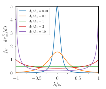
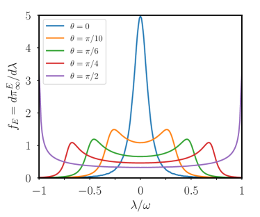
(a)	(b)

Figure 2: Non-vanishing density $f_{E}$ for eigenvalues $\lambda\in[-\omega,+\omega]$ obtained from theorem 7.1. (a) Formula (13) for integrable cases in axisymmetric ellipsoids with $A_{1}=A_{2}=1$ and $\vec{\Omega}=(0,0,1)$. (b) Numerical evaluation of formula (11 for non-integrable cases with a tilted vector $\vec{\Omega}=(\sin\theta,0,\cos\theta)$ in an axisymmetric ellipsoid $A_{1}=A_{2}=1$ and $A_{3}=0.01$.

If $E$ is an ellipsoid of revolution with $A_{1}=A_{2}$ and $\vec{\Omega}=(0,0,1)$, the density of the measure $\pi_{\infty}^{E}$ is given by

$$f_{E}:=\frac{d\pi_{\infty}^{E}}{du}=\chi_{[-1,1]}(u)\frac{a}{2\left[u^{2}+a(1-u^{2})\right]^{3/2}},\quad\chi_{[-1,1]}(u)=\begin{cases}1&\text{if}\quad|u|\leq 1\\ 0&\text{if}\quad|u|>1\end{cases},$$ (13a–b)

where we have introduced $a={A_{3}/A_{1}}$. Formula (13) is illustrated in figure 2(a). The density is uniform in $[-1,1]$ for the round ball, but we observe that the density becomes strongly non-uniform in flattened or elongated axisymmetric ellipsoids. The density is indeed peaked near zero when $A_{3}/A_{1}\to 0$, whereas the density becomes maximum near the edge of the spectrum $|\lambda|\to\omega$ when $A_{3}/A_{1}\to\infty$. Low-frequency inertial modes (known as quasi-geostrophic modes, since they are almost invariant along the rotation axis [MJL17]) are thus favoured in prolate ellipsoids. On the contrary, inertial modes have preferentially high frequencies in flattened ellipsoids. For other configurations, formula (11) is not integrable (it generally involves elliptic integrals). Yet, the area intersection can be readily evaluated numerically (e.g. figure 2b for tilted rotation axes).

7.2 Numerical validation

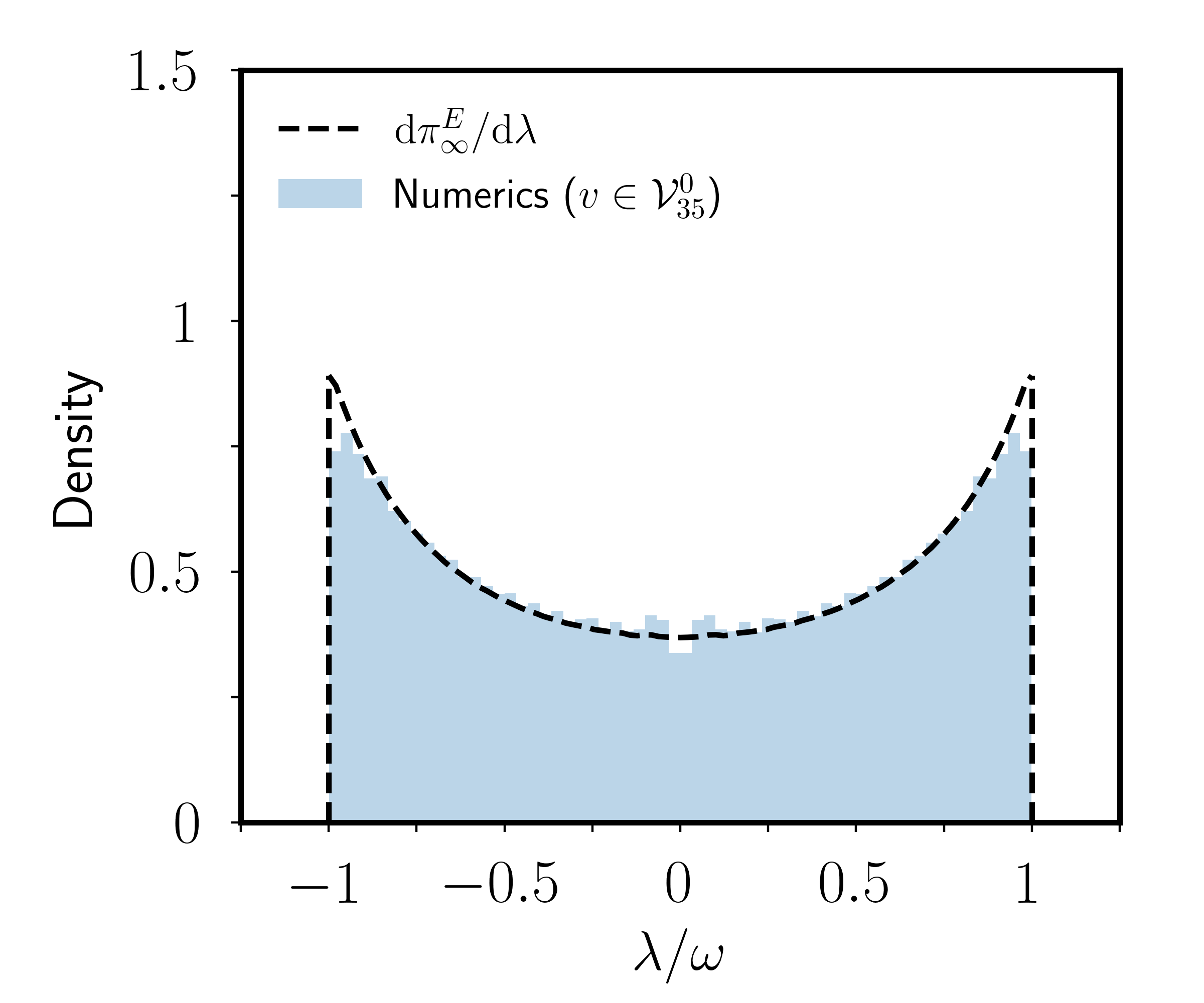
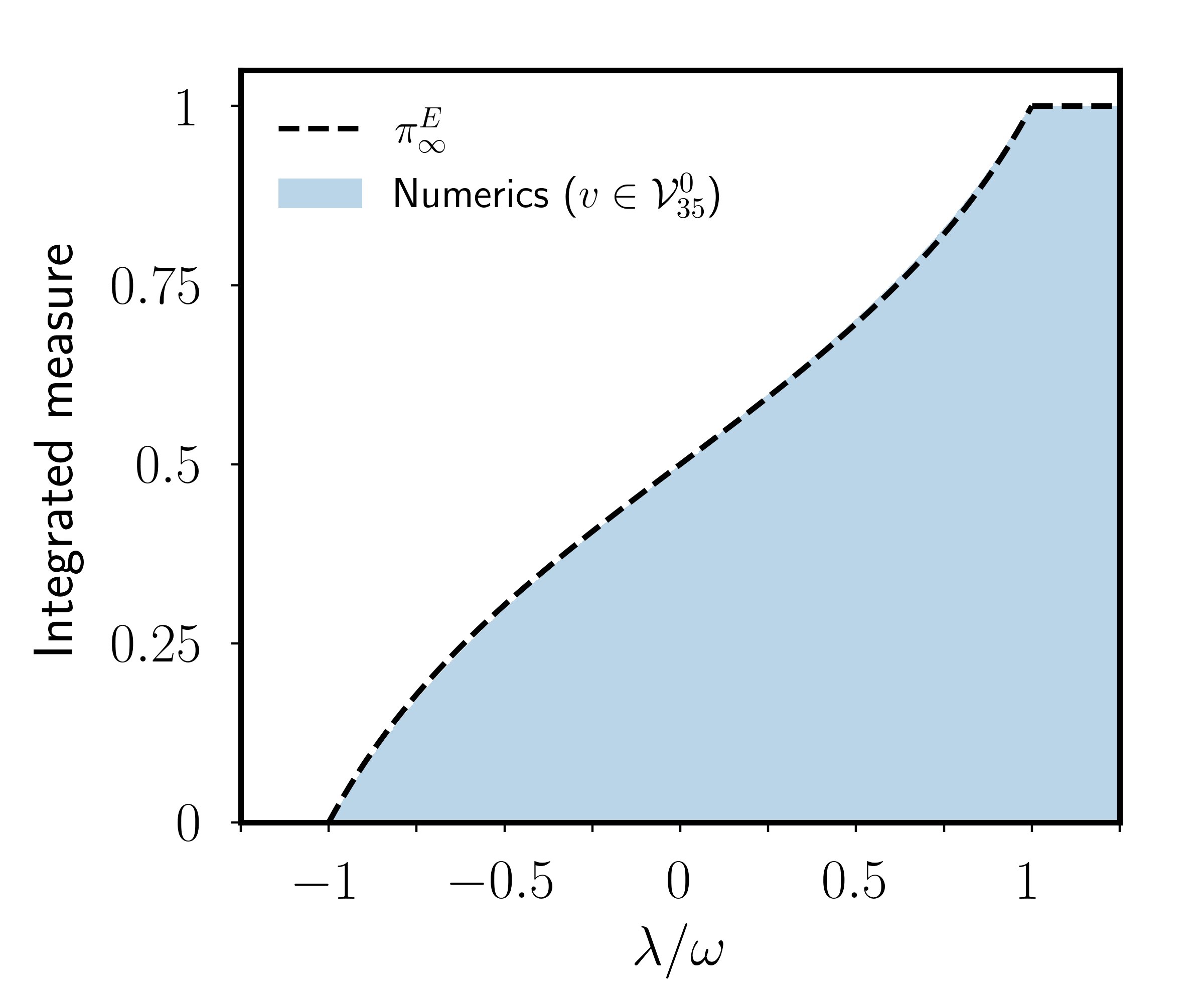
(a) Triaxial ellipsoid $A_{1}=1,\,A_{2}\simeq 1.235,\,A_{3}\simeq 2.04$ with $\theta=0$

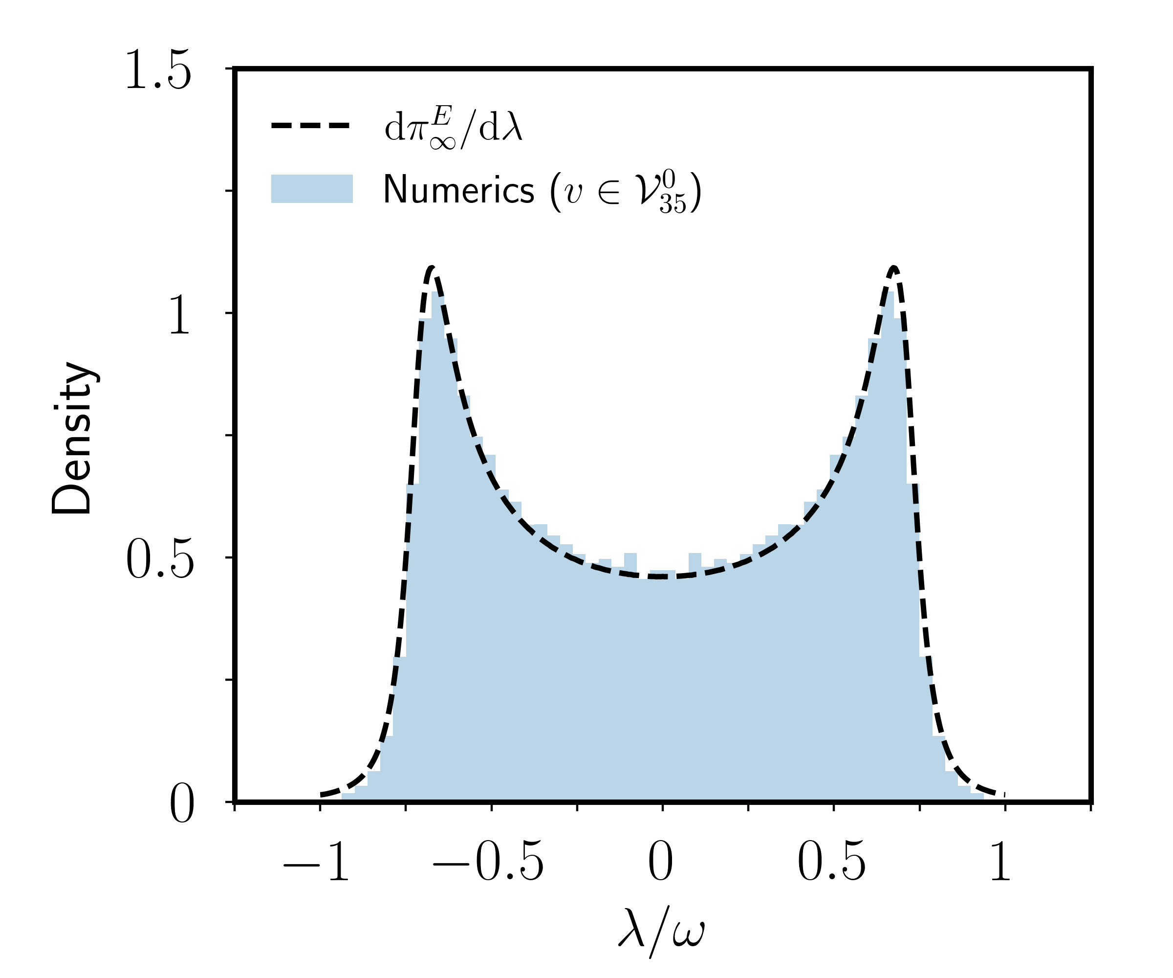
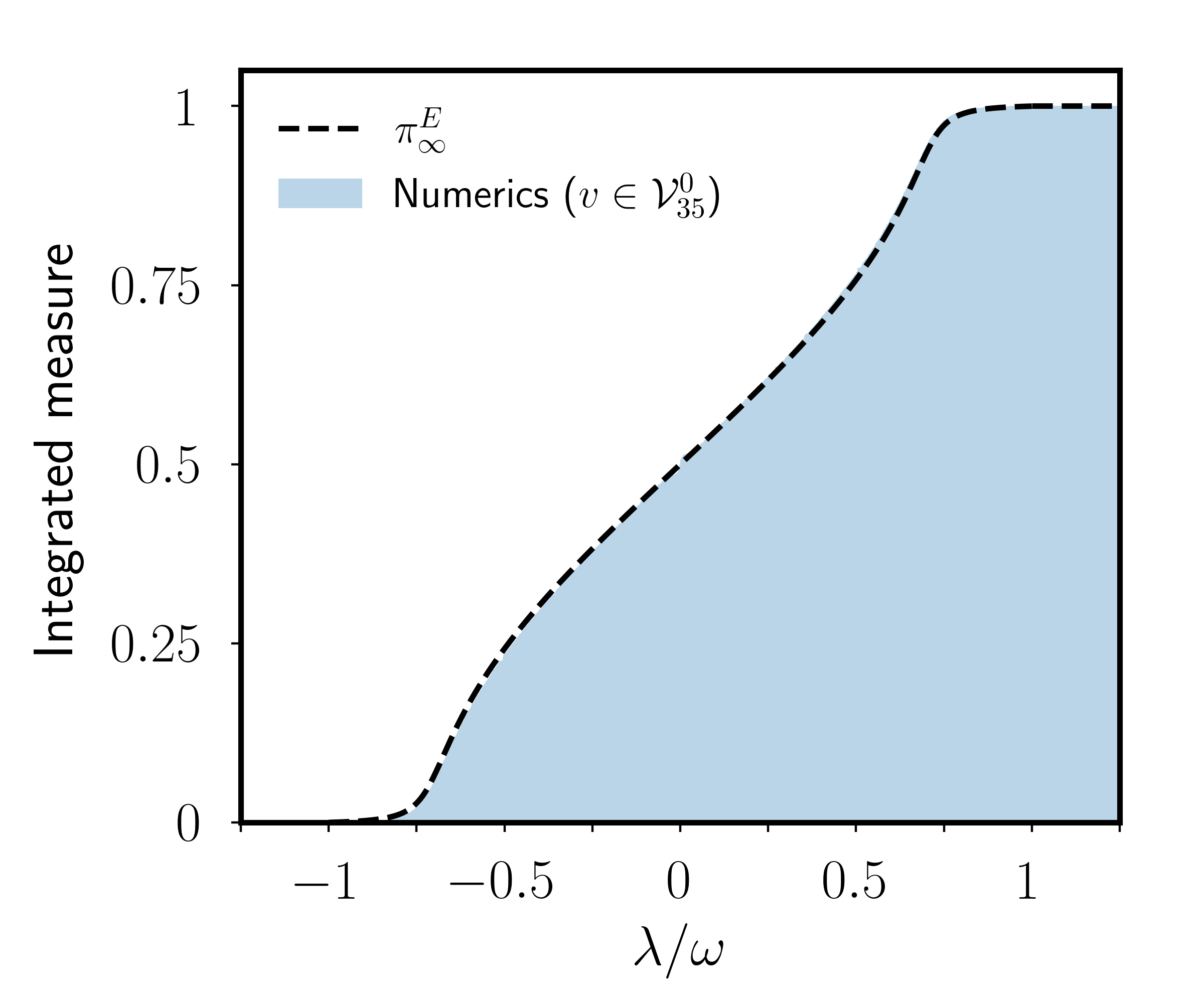
(b) Axisymmetric ellipsoid $A_{1}=A_{2}=1,\,A_{3}=0.01$ with $\theta=\pi/4$

Figure 3: Comparison between numerical computations of the full inertial-mode spectrum for $v\in{\cal V}_{35}^{0}$ and theorem 7.1 for non-integrable cases with $\vec{\Omega}=(\sin\theta,0,\cos\theta)$. Left panels: Probability densities. Right panels: Integrated probability measures.

An excellent quantitative agreement is found between formula (13) and prior computations, for both the round ball (figure 1b) and other integrable cases in axisymmetric ellipsoids (not shown). However, since formula (13) is not valid for non-integrable cases, it remains to compare theorem 7.1 with numerical computations of the inertial-mode spectrum in such cases.

To do so, every complex-valued eigenvector $v\in{\cal V}_{n}^{0}$ of equation (3) is sought using an exact polynomial expansion in ellipsoids as

$$v=\sum_{j=1}^{N}\alpha_{j}\mathfrak{e}_{j},\quad N=n(n+1)(2n+7)/{6},$$ (14a–b)

where $\{\mathfrak{e}_{j}\}_{j\leq N}$ are real-valued basis elements of ${\cal V}_{n}^{0}$ and $\vec{\alpha}=(\alpha_{1},\dots,\alpha_{B})$ contains the complex-valued coefficients of the eigenvector in the chosen basis. Different algorithms have been proposed to explicitly construct polynomial bases of ${\cal V}_{n}^{0}$, which all involve non-orthogonal basis elements in ellipsoids [Leb89, WR11, Ive17]. To determine the modal coefficients in expansion (14), we employ here a projection method [VC23]. We substitute expansion (14) in equation (3) and, then, we project the resulting equation onto every basis element $\mathfrak{e}_{i}$ such that

$$i\lambda\sum_{j=1}^{N}\alpha_{j}\int_{E}\langle\mathfrak{e}_{j},\mathfrak{e}_{i}\rangle\,dx_{1}dx_{2}dx_{3}=-\sum_{j=1}^{N}2\alpha_{j}\int_{E}\langle\vec{\Omega}\times\mathfrak{e}_{j},\mathfrak{e}_{i}\rangle\,dx_{1}dx_{2}dx_{3},$$

where the volume integration is performed analytically in ellipsoids [Leb89]. This procedure gives an exact system of equations that can be written in the form of a generalized eigenvalue problem as $A\vec{\alpha}=i\lambda B\vec{\alpha}$, where $[A,B]$ are $N\times N$ real-valued matrices. The matrix B is definite positive but, since the basis elements are not mutually orthogonal in ellipsoids, it is not diagonal. Moreover, the two matrices $[A,B]$ can become ill-conditioned for some polynomial degrees (usually when $n\geq 20$, as also found in prior studies using Cartesian polynomial expansions in ellipsoids [GJNV20, VC21]). Thus, we have solved the eigenvalue problem using extended floating-point precision (when required).

As shown in figure 3, a very good quantitative agreement is obtained for non-integrable cases between the asymptotic measure $\pi_{\infty}^{E}$ and the numerics. Therefore, theorem 7.1 can be used to obtain the asymptotic behaviour of the inertial-mode spectrum for any configuration.

8 Ray dynamics

As usual the classical (ray) dynamics gives a good way to approach the eigenmodes of large degrees. Hence, we show below a “classical version” of Theorem 2.1.

We define the ray dynamics associated to the Poincaré operator. We consider the Hamiltonians $\pm\Lambda_{1}(\xi)$ defined in Section 6. The trajectories inside $B$ are lines because the Hamiltonians are independent of $x$. There is a reflexion when a trajectory hits the boundary; we re-start there with the Hamiltonian field associated to opposite eigenvalue. The law of reflexion is not trivial. Let us consider, at energy $\lambda$, the dispersion relation $\Sigma$ that is obtained as the zero set of the determinant of the symbol of $P-\lambda$: we have $\Sigma=\{\lambda\|\xi\|^{2}-\omega\xi_{3}^{2}=0\}$. We assume that a trajectory $(x_{-}(t),\xi_{-})$ of the Hamiltonian $\Lambda_{1}$ hits the boundary at the point $m$ with the normal $\vec{n}$ to it. Then, the reflected trajectory is $(x_{+}(t),\xi_{+})$ where $\xi_{+}$ is determined by $\xi_{+}\neq\xi_{-}$, $\xi_{+}\in\Sigma$ and $(\xi_{+}-\xi_{-})(\vec{n})=0$ (recall that the $\xi$’s are linear forms on ${\mathbb{R}}^{3}$). The commutation of $P$ and $L$ implies the fact that the Poisson bracket of their principal symbols vanishes. Hence, $\sigma(L)$ is a first integral of the motion. On the other hand, the dispersion relation implies that $|\xi_{3}|/\|\xi\|$ is a constant along each trajectory. This fact can be proved directly using the law of reflexion we have just described. This proves that the classical ray dynamics admits a constant of motion. If we were in dimension $2$, we would have an integable Hamiltonian system.

9 Perspectives

The following related questions are of some interest from a mathematical viewpoint.

1. An inverse spectral problem: does the measure $\pi_{\infty}$ determine the pair $(E,\vec{\Omega})$ up to dilation of $E$?

2. What is the asymptotic behaviour of the eigenvalues when the ellipsoid degenerates to a 1-D or 2-D limit?

3. What is the asymptotic behaviour, as $n\rightarrow\infty$, of the first eigenvalues $\lambda_{j}^{n}$ for fixed $j\geq 1$ whose limits are $-\omega$?

4. Are the non-zero eigenvalues of $P$ of finite multiplicities and, hence, all eigenfunctions polynomials? In case the answer is negative or unknown, are all eigenfunctions smooth?

5. Are there other examples of integrable cases than ellipsoids of revolution with $\vec{\Omega}$ on the axis of revolution?

Finally, the mathematical analysis presented in this study could also be used to better understand the properties of other linear wave motions, such as in non-rotating stably stratified fluids (i.e. having a stable density profile $\rho$ such that $\langle\nabla\rho,\vec{g}\rangle>0$ for incompressible fluids, where $\vec{g}$ is the gravity field). Indeed, there is a strong analogy between uniformly rotating fluids and stably stratified fluids [Ver70], and the analogue of $\omega$ for stratified flows is called the Brunt-Väisälä frequency $N$. The buoyancy force can sustain internal gravity waves in stratified fluids [Lig78], which usually exhibit singular spatial structures called attractors in bounded domains [DRV99, CdVSR20]. However, if we assume that $N$ and $\vec{g}$ are spatially uniform in the fluid (with $g:=||\vec{g}||$), the pressure associated with a divergenceless velocity field is given by [RN99]

$$\nabla^{2}p=\frac{N^{2}}{g^{2}(N^{2}-\lambda^{2})}(\vec{g}\cdot\nabla)^{2}p,$$ (15)

which is very similar to Poincaré equation (4a). Therefore, under these assumptions, internal gravity waves will admit smooth polynomial solutions in ellipsoids without any attractor. This will be the subject of a future work.

Appendix A The bicharacteristic flow of $\Lambda$ and the geodesic flow on $S^{3}$

Let us introduce the maps $j_{\pm}:B\rightarrow S^{3}\subset{\mathbb{R}}^{3}_{x}\times{\mathbb{R}}_{z}$ defined by $j_{\pm}(x)=(x,z=\pm\sqrt{1-r^{2}})$ with $r=\|x\|$. We have

$$h=j_{\pm}^{\star}(dx_{1}^{2}+dx_{2}^{2}+dx_{3}^{2}+dz^{2})=dx_{1}^{2}+dx_{2}^{2}+dx_{3}^{2}+\frac{r^{2}}{1-r^{2}}dr^{2}.$$

Because of the invariance by the rotations in ${\mathbb{R}}^{3}$, we can restrict the computation of the dual metric to the points $(x_{1},0,0)$, where $h=\frac{1}{1-x_{1}^{2}}dx_{1}^{2}+dx_{2}^{2}+dx_{3}^{2}$, hence the Hamiltonian $h^{\star}=(1-x_{1}^{2})\xi_{1}^{2}+\xi_{2}^{2}+\xi_{3}^{2}$ which is equal to $\Lambda(x_{1},0,0;\xi)$. This proves that the Hamiltonian flow $\phi_{t}$ of $\Lambda$ is the projection of the geodesic flow of $S^{3}$. The geodesics of $S^{3}$ (which are not meridians) project onto ellipses in $\bar{B}$ tangent to $\partial B$ at two antipodal points. This part of the flow is simply periodic of period $2\pi$. The meridian great circles project onto a diameter, hitting the boundary at characteristic points of $\partial B$.

Appendix B A simple Tauberian Theorem

Lemma B.1

Let $Z(t)=\sum_{n\in{\mathbb{Z}}}a_{n}e^{it(n+3/2)}$ be an antiperiodic distribution on ${\mathbb{R}}$. Assume that the singular support of $Z$ is $2\pi{\mathbb{Z}}$ and that, for a function $\rho\in C_{o}^{\infty}(]-2\pi,2\pi[)$ with $\rho\equiv 1$ near $t=0$, the Fourier transform of $\rho Z$ is

$$\widehat{\rho Z}(\tau)=b(\tau).$$

Then we have $a_{n}=b(n+3/2)+O\left(n^{-\infty}\right)$.

Proof.– The asymptotics of the Fourier transform $\widehat{\rho Z}(\tau)$ is independent of $\rho$: changing $\rho$ modifies $\rho Z$ by a smooth compactly supported function whose series has a rapid decay. We can choose $\rho=\rho_{0}$ so that $\sum_{n\in{\mathbb{Z}}}\rho_{0}(t+2\pi n)=1$: assuming that $[-\pi,\pi]\subset{\rm Support}(\rho)$, we take

$$\rho_{0}(t)=\rho(t)/\sum_{n\in{\mathbb{Z}}}\rho(t+2k\pi).$$

The Fourier coefficients of $Z$ are

$$a_{n}=\frac{1}{2\pi}\int_{0}^{2\pi}e^{-it(n+3/2)}Z(t)dt=\frac{1}{2\pi}\int_{\mathbb{R}}e^{-it(n+3/2)}\rho_{0}(t)Z(t)dt=b(n+3/2)+O\left(n^{-\infty}\right).$$

$\square$

Appendix C The boundary pseudo-differential operator  calculus of Boutet de Monvel

The pseudo-differential boundary operator  are operators on functions on $B$ of the form $u\rightarrow Au:=P\tilde{u}+G\tilde{u}$ where $\tilde{u}$ is the extension of $u$ by $0$ outside $\bar{B}$ and

1. $P$ is a (classical) pseudo-differential operator  in some neighbourhood   of $\bar{B}$ satisfying the transmission property; this property is satisfied for differential operators and their parametrices.

2. $G$ is an integral operator sending functions into smooth functions in $B$ and functions smooth near $\partial B$ into smooth functions.

What will be important for us is that such operators form an algebra: the pseudo-differential operator  parts $P$ compose with the usual rules; if $\Delta$ is an elliptic operator with elliptic boundary conditions, then the parametrix of $\Delta$ is of the previous form.

Our basic example is the Leray projector $\Pi=dd^{\star}\Delta^{-1}$ where $\Delta=dd^{\star}+d^{\star}d$ is the Hodge-de Rham laplacian with relative boundary conditions: if $j:\partial B\rightarrow\bar{B}$ is the embedding, we ask that the $2$-forms $\omega$ satisfy $j^{\star}\omega=0,~{}j^{\star}(d^{\star}\omega)=0$. Recall that $\Delta$ is invertible: the kernel of $\Delta$ is isomorphic to the space $H^{2}_{\rm rel}(B,\partial B;{\mathbb{R}})$ which vanishes, because $B$ is simply connected and the Poincaré duality. The Poincaré operator is a composition of Leray projectors and a wedge product by $\vec{\Omega}$ hence belongs also to this algebra.

Appendix D A short review about the calculus of wave-front sets

For more details on this section, one can look at section 2.5 in [Hör71] or section in 1.3[DH96]. Let us simply recall that, if $u$ is a Schwartz distribution on a smooth manifold $X$, one can define the wave-front set $WF(u)$ of $u$ as a closed conical subset of $T^{\star}X\setminus 0$ whose projection onto $X$ is the singular support of $X$.

If $A:C_{o}^{\infty}(Y)\rightarrow{\cal D}^{\prime}(X)$ is a linear operator, one can look at the Schwartz kernel $[A]$ of $A$ which is a distribution on $X\times Y$. It is then natural to define $WF^{\prime}(A):=\{(x,\xi;y,\eta)\in T^{\star}(X\times Y)|(x,\xi;y,-\eta)\in WF([A])\}$. If $WF^{\prime}(A)\subset T^{\star}(X)\setminus 0\times T^{\star}(Y)\setminus 0$, one has for any $u\in{\cal D}^{\prime}(Y)$, $WF(Au)\subset WF^{\prime}(A)\circ WF(u)$.

Hörmander [Hör71] introduced what is called Fourier Integral Distributions associated to a conic Lagrangian manifold $Z$. Such distributions are defined as oscillatory integrals of the form

$$u(x)=\int_{{\mathbb{R}}^{N}}e^{i\phi(x,\theta)}a(x,\theta)|d\theta|,$$

where $\phi$ is “generating function” of $Z$ and $a$ is a symbol. There exists $m\in{\mathbb{R}}$ so that, for any multi-indices $\alpha,\beta$, there exists $C_{\alpha,\beta}>0$ so that

$$|D_{x}^{\alpha}D_{\theta}^{\beta}|(x,\theta)\leq C_{\alpha,\beta}|\theta|^{m-|\beta|}.$$

If $u$ is such a distribution, then we have $WF(u)\subset Z$.

Aknowledgements

Many thanks to Charles Epstein, Suresh Eswarathasan, Gerd Grubb, Cyril Letrouit, Johannes Sjöstrand, Andras Vasy, Bernard Valette, Jared Wunsch, Yuan Xu for answers to our questions and comments about preliminary versions. J.V. also acknowledges David Cébron for fruitful discussions about the inertial modes over the years. J.V. would like to dedicate this work to the memory of Norman R. Lebovitz (1935-2022) and Stjin Vantieghem (1983-2023), who both revivified the topic and made pioneering contributions to the field. J.V. was partly funded by the European Research Council (erc) under the European Union’s Horizon 2020 research and innovation programme (grant agreement no. 847433, theia project).

References

- [AKdF26] Paul Appell and Joseph Kampé de Fériet. Fonctions hypergéométriques et hypersphériques: polynomes d’Hermite. Gauthier-Villars, 1926.
- [AT69] Keith D. Aldridge and Alar Toomre. Axisymmetric inertial oscillations of a fluid in a rotating spherical container. J. Fluid Mech., 37(2):307–323, 1969.
- [BdM71] Louis Boutet de Monvel. Boundary problems for pseudo-differential operators. Acta Math., 126(1):11–51, 1971.
- [BR17] George Backus and Michel Rieutord. Completeness of inertial modes of an incompressible inviscid fluid in a corotating ellipsoid. Phys. Rev. E, 95(5):053116, 2017.
- [Bry89] George Hartley Bryan. VI. The waves on a rotating liquid spheroid of finite ellipticity. Philos. Trans. R. Soc. London A, 180:187–219, 1889.
- [Car22] Élie Cartan. Sur les petites oscillations d’une masse fluide. Bull. Sci. Math., 46:317–369, 1922.
- [CdV79] Yves Colin de Verdière. Sur le spectre des opérateurs elliptiques à bicaractéristiques toutes périodiques. Comment. Math. Helvetici, 54:508–522, 1979.
- [CdVSR20] Yves Colin de Verdière and Laure Saint-Raymond. Attractors for two-dimensional waves with homogeneous hamiltonians of degree 0. Comm. Pure Appl. Math., 73(2):421–462, 2020.
- [Cha69] Subrahmanyan Chandrasekhar. Ellipsoidal Figures of Equilibrium. Dover Publications, 1969.
- [CVS+21] David Cébron, Jérémie Vidal, Nathanaël Schaeffer, Antonin Borderies, and Alban Sauret. Mean zonal flows induced by weak mechanical forcings in rotating spheroids. J. Fluid Mech., 916:A39, 2021.
- [Den59] R Denchev. On the spectrum of an operator. Dokl. Akad. Nauk SSSR, 126(2):259–262, 1959.
- [DG75] Johannes Jisse Duistermaat and Victor W. Guillemin. The spectrum of positive elliptic operators and periodic bicharacteristics. Invent. Math., 29:39–79, 1975.
- [DH96] Johannes Jisse Duistermaat and Lars Hormander. Fourier Integral Operators, volume 2. Springer, 1996.
- [DRV99] Boris Dintrans, Michel Rieutord, and Lorenzo Valdettaro. Gravito-inertial waves in a rotating stratified sphere or spherical shell. J. Fluid Mech., 398:271–297, 1999.
- [DX01] Charles F. Dunkl and Yuan Xu. Orthogonal Polynomials of Several Variables. Cambridge University Press, 2001.
- [Gal11] Giovanni P. Galdi. An introduction to the mathematical theory of the Navier-Stokes equations: Steady-state problems. Springer, 2011.
- [GFLBA17] Alexander M. Grannan, Benjamin Favier, Michael Le Bars, and Jonathan M. Aurnou. Tidally forced turbulence in planetary interiors. Geophys. J. Int., 208(3):1690–1703, 2017.
- [GJNV20] Felix Gerick, Dominique Jault, Jérome Noir, and Jérémie Vidal. Pressure torque of torsional Alfvén modes acting on an ellipsoidal mantle. Geophys. J. Int., 222(1):338–351, 2020.
- [Gre68] Harvey P. Greenspan. The Theory of Rotating Fluids. Cambridge University Press, 1968.
- [Gru08] Gerd Grubb. Distributions and Operators. Springer, 2008.
- [Hör68] Lars Hörmander. The spectral function of an elliptic operator. Acta Math., 121:193–218, 1968.
- [Hör71] Lars Hörmander. Fourier integral operators. I. Acta Math., 127(1-2):79–183, 1971.
- [Ive17] David J. Ivers. Enumeration, orthogonality and completeness of the incompressible Coriolis modes in a tri-axial ellipsoid. Geophys. Astrophys. Fluid Dyn., 111(5):333–354, 2017.
- [Kel80] Lord Kelvin. Vibrations of a columnar vortex. Phil. Mag., 10:155–168, 1880.
- [Ker02] Richard. R. Kerswell. Elliptical instability. Annu. Rev. Fluid Mech., 34(1):83–113, 2002.
- [Kud66] M. D. Kudlick. On transient motions in a contained, rotating fluid. PhD thesis, Massachusetts Institute of Technology, 1966.
- [LBCLG15] Michael Le Bars, David Cébron, and Patrice Le Gal. Flows driven by libration, precession, and tides. Annu. Rev. Fluid Mech., 47:163–193, 2015.
- [Leb89] Norman R. Lebovitz. The stability equations for rotating, inviscid fluids: Galerkin methods and orthogonal bases. Geophys. Astrophys. Fluid Dyn., 46(4):221–243, 1989.
- [Lig78] James Lighthill. Waves in Fluids. Cambridge University Press, 1978.
- [Lin21] Yufeng Lin. Triadic resonances driven by thermal convection in a rotating sphere. J. Fluid Mech., 909:R3, 2021.
- [LRFLB19] Thomas Le Reun, Benjamin Favier, and Michael Le Bars. Experimental study of the nonlinear saturation of the elliptical instability: inertial wave turbulence versus geostrophic turbulence. J. Fluid Mech., 879:296–326, 2019.
- [MJL17] Stefano Maffei, Andrew Jackson, and Philip W. Livermore. Characterization of columnar inertial modes in rapidly rotating spheres and spheroids. Proc. R. Soc. A, 473(2204):20170181, 2017.
- [NC13] Jérome Noir and David Cébron. Precession-driven flows in non-axisymmetric ellipsoids. J. Fluid Mech., 737:412–439, 2013.
- [Poi85] Henri Poincaré. Sur l’équilibre d’une masse fluide animée d’un mouvement de rotation. Acta Math., 7:259–380, 1885.
- [RFLB18] K. Sandeep Reddy, Benjamin Favier, and Michael Le Bars. Turbulent kinematic dynamos in ellipsoids driven by mechanical forcing. Geophys. Res. Lett., 45(4):1741–1750, 2018.
- [RGV00] Michel Rieutord, Bertrand Georgeot, and Lorenzo Valdettaro. Wave attractors in rotating fluids: a paradigm for ill-posed Cauchy problems. Phys. Rev. Lett., 85(20):4277, 2000.
- [RN99] Michel Rieutord and Karim Noui. On the analogy between gravity modes and inertial modes in spherical geometry. Eur. Phys. J. B, 9:731–738, 1999.
- [RV10] Michel Rieutord and Lorenzo Valdettaro. Viscous dissipation by tidally forced inertial modes in a rotating spherical shell. J. Fluid Mech., 643:363–394, 2010.
- [TGBR22] Santiago Andres Triana, Gustavo Guerrero, Ankit Barik, and Jérémy Rekier. Identification of inertial modes in the solar convection zone. Astrophys. J. Lett., 934(1):L4, 2022.
- [Van14] Stjin Vantieghem. Inertial modes in a rotating triaxial ellipsoid. Proc. R. Soc. A, 470(2168):20140093, 2014.
- [VC21] Jérémie Vidal and David Cébron. Kinematic dynamos in triaxial ellipsoids. Proc. R. Soc. A, 477(2252):20210252, 2021.
- [VC23] Jérémie Vidal and David Cébron. Precession-driven flows in stress-free ellipsoids. J. Fluid Mech., 954:A5, 2023.
- [VCN15] Stjin Vantieghem, David Cébron, and Jérome Noir. Latitudinal libration driven flows in triaxial ellipsoids. J. Fluid Mech., 771:193–228, 2015.
- [VCSH18] Jérémie Vidal, David Cébron, Nathanaël Schaeffer, and Rainer Hollerbach. Magnetic fields driven by tidal mixing in radiative stars. Mon. Not. R. Astron. Soc., 475(4):4579–4594, 2018.
- [Ver70] George Veronis. The analogy between rotating and stratified fluids. Annu. Rev. Fluid Mech., 2(1):37–66, 1970.
- [VSC20] Jérémie Vidal, Sylvie Su, and David Cébron. Compressible fluid modes in rigid ellipsoids: towards modal acoustic velocimetry. J. Fluid Mech., 885:A39, 2020.
- [Wei77] Alan Weinstein. Asymptotics of eigenvalue clusters for the Laplacian plus a potential. Duke Math. J., 44(1):883–892, 1977.
- [WR11] Cheng-Chin Wu and Paul H. Roberts. High order instabilities of the Poincaré solution for precessionally driven flow. Geophys. Astrophys. Fluid Dyn., 105(2-3):287–303, 2011.
- [Zha94] Keke Zhang. On coupling between the Poincaré equation and the heat equation. J. Fluid Mech., 268:211–229, 1994.
- [ZL17] Keke Zhang and Xinhao Liao. Theory and Modeling of Rotating Fluids: Convection, Inertial Waves and Precession. Cambridge University Press, 2017.