Albert Munyeshyaka¹,Joseph Ntahompagaze²,Tom Mutabazi¹ and Manasse.R Mbonye<sup>2,3,4

1</sup>Department of Physics, Mbarara University of Science and Technology, Mbarara, Uganda       
²Department of Physics, College of Science and Technology, University of Rwanda, Rwanda       
³ International Center for Theoretical Physics (ICTP)-East African Institute for Fundamental Research, University of Rwanda, Kigali, Rwanda        
⁴ Rochester Institute of Technology, NY, USA.


Correspondence:munalph@gmail.com

Abstract

The consideration of a $1+3$ covariant approach to cold dark matter universe with no shear cosmological dust model with irrotational flows is developed in the context of $f(G)$ gravity theory in the present study. This approach reveals the existence of integrability conditions which do not appear in non-covariant treatments. We constructed the integrability conditions in modified Gauss-Bonnet $f(G)$ gravity basing on the constraints and propagation equations. These integrability conditions reveal the linearized silent nature of quasi-Newtonian models in $f(G)$ gravity. Finally, the linear equations for the overdensity and velocity perturbations of the quasi-Newtonian space-time were constructed in the context of modified $f(G)$ gravity. The application of harmonic decomposition and redshift transformation techniques to explore the behaviour of the overdensity and velocity perturbations using $f(G)$ model were made. On the other hand we applied the quasi-static approximation to study the approximated solutions on small scales which helps to get both analytical and numerical results of the perturbation equations. The analysis of the energy overdensity and velocity perturbations for both short and long wavelength modes in a dust-Gauss-Bonnet fluids were done and we see that both energy overdensity and velocity perturbations decay with redshift for both modes. In the limits to $\Lambda CDM$, it means $f(G)=G$ the considered $f(G)$ model results coincide with $\Lambda CDM$.

keywords: $1+3$ covariant formalism– cosmic acceleration– Cosmological perturbations– Quasi-newtonian spacetime.
PACS numbers: 04.50.Kd, 98.80.-k, 95.36.+x, 98.80.Cq; MSC numbers: 83F05, 83D05

1 Introduction

Different astrophysical and cosmological observations confirm the cosmic acceleration [1, 2]. The nature of the substance behind this current cosmic accelaration is still unkown [3, 4]. It is therefore necessary to modify General Relativity(GR) for the sake of explaining this cosmic acceleration. Currently, the most popular idea is that the energy density of the universe is dominated by dark component dubbed dark energy and to astrophysical scale, dark matter and many proposals are drafted to explain their nature. The concordance model of cosmology appears to fit the present observations such as supernova Ia, cosmic microwave background anisotropy, large-scale structure formation, baryon accoustic oscillation and weak lensing to mention a few. This concordance model relies on the cosmological constant and cold dark matter ($\Lambda CDM$)[30, 5, 6, 7, 9]. However, despite its success the $\Lambda CDM$ model is affected by its inability to address problems like the large-scale structure formation and evolution, the cosmic acceleration among many others. Addressing cosmic acceleration problem, other exotic negative pressure fluids, described in terms of scalar fields have been taken into consideration. However at present, there is no evidence for the existence of the scalar fields responsible for the late-time accelerated expansion of the universe. This led to the searches for other viable theoretical avenues many of which are based on the idea that the dark sector originates from modification of the gravitational interactions[11]. Currently one of the most popular alternative to the concordance model is the modification of the Einstein-Hilbert action from which the dark energy may have a geometrical origin.

In line with that, modified gravity theories have extensively been explored to explain different cosmological scenarios including large-scale structure formation and cosmic accelaration. The most popular modified theories of gravity include $f(R)$[12, 13, 14, 15], $R$ being the Ricci scalar, $f(T)$ [16, 17, 18], $T$ being the torsion scalar, $f(Q)$ [19, 20, 21, 22, 23, 24], $Q$ being nonmetricity scalar and $f(G)$[25, 3, 26, 27] models, $G$ being the Gauss-Bonnet invariant. One advantage of $f(T)$ gravity is that the field equations are second order in the metric. But the $f(T)$ gravity does not respect the local lorentz invariance unless replacing the partial derivative by lorentz covariant derivative in the definition of the torsion tensor to get new torsion scalar [16]. One advantage of $f(G)$ gravity is that the Energy Momentum Tensor(EMT) decouples from the correction term. In other modified gravity theories, the correction terms modify the EMT. The constructon of viable $f(R)$ or $f(T)$ models that are consistent with cosmological and GR constraints seems to be difficult since these modified theories of gravity give rise to a strong coupling between dark energy and a non-relativistic matter in the Einstein frame [28, 29]. The goal is to explain both the early and the late-time acceleration in a geometrical way without considering the dark energy or the scalar fields[31, 32, 33]. Among these different theories, a key role in this paper is played by the Gauss-Bonnet invariant $G$. Considering a theory where both $R$ and $G$ are non-linear, exhausts the energy budget of the curvature degrees of freedom needed to modify GR. Introducing $G$ besides $R$ implies presence of two acceleration phases led by $G$ and $R$ respectively. This is possible for the non-linear combination of both $G$ and $R$ since linear $R$ reduces to GR while linear $G$ vanishes identically in four dimensional gravitational action being an invariant. The same studies on these models have been done [33, 34, 35, 36, 37] showing evidence that the Gauss-Bonnet invariant can solve some shortcomings of the original $f(R)$ and can contribute to the explanation of the accelerated cosmic expansion as well as the phantom behaviour, the quintessence behaviour and the transition from deceleration to acceleration phases and can also work at infrared scales [31]. These combinations have some shortcomings that the ghost instabilities may arise. The work done in [8] presents the absence of dark energy oscillations, which indicates the advantage of the $f(G)$ theory for the interpretation of late time phenomenology. [8] considered scalar field coupled with Ricci scalar and a function $f(G)$. In this study we choose a combination of linear $R$ and non-linear $G$ to make the $f(G)$ theories stable and able to describe the current acceleration of the universe and can be compared with the $\Lambda CDM$ for a linear $G$, that means for the case $f(G)=G$ as well as other cosmological solutions and suitable perturbation schemes[38, 39, 40, 41, 42].

In exploration of such models, there are different approaches to study cosmological perturbations such as metric formalism [43, 44, 45, 46, 47, 48] and $1+3$ covariant formalism [49, 50]. In this study, we use $1+3$ covariant formalism, a gauge-invariant formalism and the perturbation variables describe true physical degrees of freedom and no unphysical mode exists. This formalism has been extensively applied in GR [49], scalar-tensor theories[51, 52, 53] and different modified theories of gravity and in addition to that, one considers the spacetime with quasi-Newtonian features [27, 54, 12, 55, 16, 19].

Different authors have studied quasi-Newtonian cosmologies in GR limits, scalar-tensor theories and $f(R)$ in the context of large-scale structure formation and non-linear gravitational collapse in the late universe[56, 57, 58, 59]. The importance of investigating the quasi-Newtonian models for general relativity in cosmological context is that there is a viewpoint in which cosmological studies can be done using Newtonian physics with the relativistic theory only needed for examination of different observational predictions.

Apart from that, modified theories of gravity such as $f(R)$ and $f(G)$ have been shown to exhibit more shared properties with quasi-Newtonian gravitation than GR does. A covariant approach to cold matter universe in quasi-Newtonian cosmologies has been developed in order to derive and solve the equations governing density and velocity perturbations [57, 61, 58, 62]. This approach revealed the existence of integrability conditions in GR and $f(R)$ models. In this paper we derive the integrability conditions and study the velocity and density perturbations in the context of $f(G)$ gravity for large-scale structure formation.

On the other hand, the velocity and density perturbations are important to the explanation of the large scale structure formation scenario. The covariant and gauge-invariant approach to perturbations instituted by Ellis and Bruni [49] will be used since it is very important that all quantities have a direct and immediate geometrical meaning and no non-local decomposition for example into scalar modes required and this approach provides a natural and transparent settings to search for integrability conditions which may arise from constraint equations[57, 63, 56, 64]. Furthermore, there is a need to study a quasi-Newtonian spacetime perturbations in $f(G)$ gravity since it will help to reveal the integrability conditions and to analyse velocity and energy density perturbation and check the large scale structure formation scenarios. The aim of this paper is therefore to present the framework for studying cosmological perturbations of the quasi-newtonian spacetime in $f(G)$ gravity using the $1+3$ covariant formalism.

In this paper, we solve the whole system of velocity and energy density perturbation equations for both GR and $f(G)$ gravity. For comparison purpose, we observe that the energy density perturbations with redshift decay for both GR and $f(G)$ gravity. On the other side, we apply quasi-static approximation method where very slow temporal fluctuations is considered in the perturbations for both Gauss-Bonnet energy density and momentum compared with the fluctuations of matter energy density. In this approximation, the time derivative terms of the fluctuations for Gauss-Bonnet energy density and momentum are discarded. The present work reveals that for comparison, the energy density and velocity perturbations decay with redshift for the considered $f(G)$ gravity model.

The rest of this paper is organised as follows: in Sec. 2 we give background field equations in modified $f(G)$ gravity and the $1+3$ Covariant description and the general propagation and constraint equations are presented. In Sec. 3, we describe the Quasi-Newtonian spacetimes in modified $f(G)$ gravity and we present the integrability conditions. In Sec. 4, we define the covariant perturbation variables for $f(G)$ gravity, derive their evolution equations and analyse their solutions. Finally in Sec. 5 we present the summary of the results and give conclusions.

Natural units in which $c=8\pi G_{N}=1$ will be used throughout this paper, and Greek indices run from 0 to 3. The symbols $\nabla$, $\tilde{\nabla}$ and the overdot ^. represent the usual covariant derivative, the spatial covariant derivative, and differentiation with respect to cosmic time, respectively. We use the $(-+++)$ spacetime signature.

2 Background field equations and the $1+3$ covariant equations in modified $f(G)$ gravity

The modified Gauss-Bonnet gravity action with matter field contribution to the Lagrangian, ${\cal L}_{m}\;,$ is given by[25, 67, 38, 26, 68]

$$\mathcal{S}=\frac{1}{2}\int d^{4}x\sqrt{-g}\left[R+f(G)+2\mathcal{L}_{m}\right]\;,$$ (1)

with $\kappa$ is assumed to equals to $1$. The modified Einstein equation is presented as

$$R_{\mu\nu}-\frac{1}{2}g^{\mu\nu}R=T^{m}_{\mu\nu}+\frac{1}{2}g^{\mu\nu}f-2f^{\prime}RR^{\mu\nu}+4f^{\prime}R^{\mu}_{\lambda}R^{\nu\lambda}-2f^{\prime}R^{\mu\nu\sigma\tau}R^{\lambda\sigma\tau}_{b}$$

$$-4f^{\prime}R^{\mu\lambda\sigma\nu}R_{\lambda\sigma}+2R\bigtriangledown^{\mu}\bigtriangledown_{\nu}f^{\prime}-2Rg^{\mu\nu}\bigtriangledown^{2}f^{\prime}-4R^{\nu\lambda}\bigtriangledown_{\lambda}\bigtriangledown^{\mu}f^{\prime}$$

$$-4R^{\mu\lambda}\bigtriangledown_{\lambda}\bigtriangledown^{\nu}f^{\prime}+4R^{\mu\nu}\bigtriangledown^{2}f^{\prime}+4g^{\mu\nu}R^{\lambda\sigma}\bigtriangledown_{\lambda}\bigtriangledown_{\sigma}f^{\prime}-4R^{\mu\lambda\nu\sigma}\bigtriangledown_{\lambda}\bigtriangledown_{\sigma}f^{\prime},$$ (2)

where $f\equiv f(G)$ and $f^{\prime}=\frac{\partial f}{\partial G}$ and $T^{m}_{\mu\nu}$ is the energy momentum tensor of the fluid matter (photons, baryons, cold dark matter, and light neutrinos) with $G$ is the Gauss-Bonnet term given as $R^{2}-4R_{\mu\nu}R^{\mu\nu}+R_{\mu\nu\alpha\beta}R^{\mu\nu\alpha\beta}$, $R=R(g_{\mu\nu})$ is the Ricci scalar, $R^{\mu\nu}$ is the Ricci tensor and $R^{\mu\nu\alpha\beta}$ is the Riemann tensor. In this paper, we use $1+3$ covariant formalism where a spacetime is assumed to have timelike congruence thus tensors can be splitted into temporal and spatial parts with respect to the congruence [65]. The $1+3$ formalism relies on the slicing of the four dimensional spacetime by time and space(hypersurfaces) as far as GR and Einsteins equations are concerned. For congruence normal to a spacelike hypersurface, the $1+3$ formalism reduces to $3+1$ formalism [66]. The basic structure of $1+3$ formalism is a congruence of one dimensional curves mostly timelike curve, it means worldlines instead of a family of three-dimensional surfaces as in the $3+1$ formalism case [65, 66]. In the $1+3$ formalism, we decompose spacetime cosmological manifold $(M,g)$ into time and space submanifold $(M,h)$ separately with a perpendicular 4-velocity field vector $u^{a}$ so that the 4-velocity field vector $u^{a}$ is defined as [69, 50, 53]

$$u^{a}=\frac{dx^{a}}{d\tau},$$

where $\tau$ is the proper time such that $u^{a}u_{a}=-1$. The metric $g_{ab}$ is related to the projection tensor $h_{ab}$ via:

$$g_{ab}=h_{ab}-u_{a}u_{b}.$$

$u^{a}\equiv\frac{dx^{a}}{dt}$ is the $4$-velocity of fundamental observers comoving with the fluid and is used to define the covariant time derivative for any tensor ${S}^{\alpha..\beta}{}_{\gamma..\delta}$ along an observer’s worldlines:

$$\dot{S}^{\alpha..\beta}{}_{\gamma..\delta}{}=u^{\lambda}\bigtriangledown_{\lambda}{S}^{\alpha..\beta}{}_{\gamma..\delta}\;.$$ (3)

In the $4$-velocity field $u_{a}$ , the Ehlers-Ellis approach gives fully covariant quantities and equations with transparent physical and geometric meaning [58, 69, 71, 53]. The energy-momentum tensor of matter fluid forms is given by [69, 50, 53]

$$T_{\mu\nu}=\rho u_{\mu}u_{\nu}+ph_{\mu\nu}+q_{\mu}u_{\nu}+q_{\nu}u_{\mu}+\pi_{\mu\nu}\;,$$ (4)

where $\rho$, $p$, $q_{\mu}$ and $\pi_{\mu\nu}$ are the energy density, isotropic pressure, heat flux and anisotropic pressure of the fluid respectively. The first covariant derivative of $u^{a}$ can be split into its irreducible parts as

$$\bigtriangledown_{\alpha}u_{\beta}=-A_{\alpha}u_{\beta}+\frac{1}{3}\Theta h_{\alpha\beta}+\sigma_{\alpha\beta}+\epsilon_{\alpha\beta\gamma}\omega^{\gamma},$$ (5)

where $A_{\alpha}\equiv\dot{u}_{\alpha}$, $\Theta\equiv\tilde{\bigtriangledown}_{\alpha}u^{\alpha}$, $\sigma_{\alpha\beta}\equiv\tilde{\bigtriangledown}_{\langle\alpha}u_{\beta\rangle}$ and $\omega^{\alpha}\equiv\epsilon^{\alpha\beta\gamma}\tilde{\bigtriangledown}_{\beta}u_{\gamma}$. The quantities $\pi_{\mu\nu}$, $q^{\mu}$, $\rho$ and $p$ are reffered to as dynamical quantities which can be obtained from the energy momentum tensor $T_{\mu\nu}$ as

$$\rho=T_{\mu\nu}u^{\mu}u_{\nu},$$ (6)

$$p=-\frac{1}{3}h^{\mu\nu}T_{\mu\nu},$$ (7)

$$q_{\mu}=h^{\sigma}_{\mu}u^{\rho}T_{\rho\sigma},$$ (8)

$$\pi_{\mu\nu}=h^{\rho}_{\mu}h^{\sigma}_{\nu}+ph_{\mu\nu}.$$ (9)

The quantities $\sigma_{\mu\nu}$, $\varpi_{\mu\nu}$, $\theta$ and $A_{\mu}$ are reffered as kinematical quantities. The consideration of standard matter fields (dust, radiation, etc) and Gauss-Bonnet contributions leads us to define the total energy density, isotropic pressures, heat flux and the projected symmetric trace-free anisotropic stress as

$$\rho=\rho_{m}+\rho_{G},~{}p=p_{m}+p_{G},~{}q^{a}=q_{m}^{a}+q_{G}^{a},~{}\pi^{ab}=\pi_{m}^{ab}+\pi_{G}^{ab},$$ (10)

where [25, 70, 27, 8]

$$\rho_{G}=\frac{1}{2}(f^{\prime}G-f)-24f^{\prime\prime}\dot{G},$$ (11)

$$p_{G}=\frac{1}{2}(f-f^{\prime}G)+\frac{G\dot{G}}{3H}f^{\prime\prime}+4H^{2}\ddot{G}f^{\prime\prime}+4H^{2}\dot{G}^{2}f^{\prime\prime\prime},$$ (12)

$$q_{G}^{a}=-\frac{4}{9}\theta^{2}\left(f^{\prime\prime\prime}\dot{G}\bigtriangledown_{a}G+f^{\prime\prime}\bigtriangledown_{a}\dot{G}-\frac{\theta}{3}f^{\prime\prime}\bigtriangledown_{a}G\right),$$ (13)

$$\pi_{G}^{ab}=\frac{G}{2\theta}f^{\prime\prime}\bigtriangledown_{a}\bigtriangledown_{b}G+2\left(f^{\prime\prime}\ddot{G}+f^{\prime\prime\prime}\dot{G}^{2}+\frac{1}{3}\theta f^{\prime\prime}\dot{G}\right)\pi_{ab}+\frac{G}{2\theta}f^{\prime\prime}\dot{G}\sigma_{ab}$$

$$\quad\quad+\left(\frac{4}{3}\theta\dot{G}f^{\prime\prime}-4\ddot{G}f^{\prime\prime}-4f^{\prime\prime\prime}\dot{G}^{2}\right)E_{ab}.$$ (14)

For a spatially flat FRW universe we have

$$ds^{2}=-dt^{2}+a^{2}\left(dx^{2}+dy^{2}+dz^{2}\right),$$ (15)

and the equation corresponding to the Friedmann equation is presented as follows:

$$3H^{2}=\frac{1}{2}\left(Gf^{\prime}-f-24\dot{G}H^{3}f^{\prime\prime}\right)+\rho_{m}\;,$$ (16)

$$G=24H^{2}(\dot{H}+H^{2})\;,$$ (17)

$$R=6(\dot{H}+2H^{2})\;,$$ (18)

where $H=\frac{\dot{a}}{a}$ is the Hubble parameter and $a$ is the scale factor. The energy density and pressure in the modified Gauss-Bonnet gravity are presented as

$$\rho=3H^{2}\;,$$ (19)

$$p=-(3H^{2}+2\dot{H})\;.$$ (20)

The matter is considered as barotropic perfect fluid such that $p=w\rho$, where $w$ is the equation of state parameter.

2.1 Propagation equations

The covariant linearised evolution equations are given by [45, 58, 71, 59, 72, 52]

$$\dot{\theta}+\frac{1}{×3}\theta^{2}+\frac{1}{2}(\rho+p)-\tilde{\bigtriangledown}^{a}A_{\mu}=0,$$ (21)

$$\dot{\sigma}_{\mu\nu}+\frac{2}{3}\theta\sigma_{\mu\nu}+E_{\mu\nu}+\frac{1}{2}\pi_{\mu\nu}-\tilde{\bigtriangledown}_{a}A_{\nu}=0,$$ (22)

$$\dot{\varpi}^{\mu}+\frac{2}{3}\theta\varpi^{\mu}-\frac{1}{2}\eta^{\mu\nu\sigma}\tilde{\bigtriangledown}_{a}A_{\nu}=0,$$ (23)

$$\frac{1}{2}\dot{\pi}_{\mu\nu}+\frac{1}{6}\theta\pi_{\mu\nu}-\frac{1}{2}(\rho+p)\sigma_{\mu\nu}-\frac{1}{2}\tilde{\bigtriangledown}_{a}q_{\mu}-\dot{E}_{\mu\nu}-\theta E_{\mu\nu}+\eta^{\rho\sigma}\tilde{\bigtriangledown}_{a}H^{\nu}_{\sigma}=0,$$ (24)

$$\dot{H}_{\mu\nu}+\theta H_{\mu\nu}+\eta^{\rho\sigma}\tilde{\bigtriangledown}_{\rho}E^{\nu}_{\sigma}+\frac{1}{2}\eta^{\rho\sigma}\tilde{\bigtriangledown}_{\rho}\pi^{\nu}_{\sigma}=0.$$ (25)

These equations will be used in the derivation of integrability conditions and the perturbation equations.

2.2 Constraints Equations

The covariant linearised constraint equations are given by [45, 58, 71, 59, 52]

$$\eta^{\rho\sigma}\tilde{\bigtriangledown}_{\rho}\varpi^{\nu}_{\sigma}=0,$$ (26)

$$q^{\mu}=-\frac{2}{3}\tilde{\bigtriangledown}_{\mu}\theta+\tilde{\bigtriangledown}^{\nu}\sigma_{\mu\nu}+\tilde{\bigtriangledown}^{\nu}\varpi_{\mu\nu},$$ (27)

$$H_{\mu\nu}=\eta^{\rho\sigma}[\tilde{{}^{\mu}\bigtriangledown}_{\rho}\sigma^{\rho}_{\nu}+\tilde{\bigtriangledown}^{\mu}\varpi_{\nu}],$$ (28)

$$\tilde{\bigtriangledown}^{\nu}E_{\mu\nu}=\frac{1}{2}[\tilde{\bigtriangledown}^{\mu}\pi_{\mu\nu}+\frac{2}{3}\theta q_{\mu}+\frac{2}{3}\tilde{\bigtriangledown}_{\mu}\rho],$$ (29)

$$\tilde{\bigtriangledown}^{\nu}H_{\mu\nu}=\frac{1}{2}\left[\tilde{\bigtriangledown}_{\sigma}q_{\rho}+(\rho+p)\varpi_{\sigma\rho}\right]\eta^{\mu\nu\sigma}.$$ (30)

where $\eta_{\mu\nu\sigma\rho}$ is the covariant permutation tensor, and $E_{\mu\nu}$ and $H_{\mu\nu}$ are respectively the electric and magnetic parts of the Weyl tensor responsible for tidal forces and gravitational waves. The projected Ricci scalar $\tilde{R}$ into the hypersurfaces orthogonal to $u^{a}$ is given as

$$\tilde{R}=2\rho-\frac{2}{3}\theta^{2}.$$ (31)

where $\theta=3H$. The conservation equation is

$$\dot{\rho}+(\rho+p)\theta+\tilde{\bigtriangledown}^{a}q_{a}=0.$$ (32)

The other important equation for $\dot{u}$ is given as[69, 50, 53]

$$\dot{q}_{a}+\frac{4}{3}\theta q_{a}+(\rho+p)\dot{u}_{a}-\tilde{\bigtriangledown}_{a}p+\tilde{\bigtriangledown}^{b}\pi_{ab}=0.$$ (33)

In the FRW background, the dynamic, kinematic and gravito-electromagnetic equations become

$$\tilde{\bigtriangledown}_{a}\rho=0=\tilde{\bigtriangledown}_{a}p=\tilde{\bigtriangledown}_{a}\theta,A_{a}=0=\varpi_{a}=q_{a},\pi_{ab}=0=\sigma_{ab}=E_{ab}=H_{ab}.$$ (34)

As we will assume, the spatially flat universe, no curvature on large scale, therefore $\tilde{R}=0$, hence eq. 31 deduces to

$$\frac{1}{3}\theta^{2}=\rho,$$ (35)

which is the Friedman equation in standard general relativity. The Raychaudhuri equation in modified Gauss-Bonnet gravity is presented as

$$\dot{\theta}+\frac{1}{3}\theta^{2}+\frac{1}{2}\left[(1+3w_{m})\rho_{m}+f-f^{\prime}G+\left(\frac{G\dot{G}}{H}-24\dot{G}+12H^{2}\ddot{G}\right)f^{\prime\prime}+12H^{2}\dot{G}^{2}f^{\prime\prime\prime}\right]=0.$$ (36)

3 Quasi-Newtonian spacetimes in modified $f(G)$ gravity

3.1 Introduction

The comoving $4$-velocity $\tilde{u}^{a}$ can be defined in the linearised form as,

$$\tilde{u}^{a}=u^{a}+v^{a},$$ (37)

$u_{a}u^{a}=0$, $v_{a}v^{a}\ll 1,$ so there is a change in the dynamical, kinematical and gravito-electromagnetic quantities. Here $v^{a}$ is the relative velocity of the comoving frame with respect to the observer in the quasi-Newtonian frame, defined such that it vanishes in the background. Quasi-newtonian spacetime is known to be irrotational, shear free dust characterised by [71, 57]

$$p_{m}=0,q_{a}^{m}=\rho_{m}v_{a},\pi_{ab}^{m}=0,\varpi_{a}=0,\sigma_{ab}=0.$$ (38)

The shear free $\sigma_{ab}=0$, irrotational $\varpi_{ab}=0$ and the gravito-electromagnetic constraint equation (eq. 28) result in the silent constraint

$$H_{ab}=0,$$ (39)

thus there is no gravitational radiation, implying the term ’Quasi-Newtonian’. Due to vanishing of the shear, eq. 24 becomes

$$E_{ab}=\tilde{\bigtriangledown}_{a}A_{b}-\frac{1}{2}\pi_{ab},$$ (40)

and using the identity in Eq. (98) for any scalar $\varphi$, Eq. 23 can be simplified as

$$\tilde{\bigtriangledown}_{a}A_{b}=0,$$ (41)

therefore [58, 71]

$$A_{a}=\tilde{\bigtriangledown}_{a}\varphi,$$ (42)

where $\varphi$ is the covariant relativistic generalisation of the Newtonian potential. Eqs 30 and 38 show that $q_{a}$ is irrotational and thus so $v_{a}$

$$\tilde{\bigtriangledown}_{b}~{}q_{a}=0.$$ (43)

It follows that for a vanishing vorticity, there exists a velocity potential $\psi$ such that

$$v_{a}=\tilde{\bigtriangledown}_{a}\psi.$$ (44)

In general, if the silent constraint $H_{ab}=0$ is imposed, the linear models are consistent but the non-linear models are not consistent [58, 71]. Thus the usual approach to the integrability conditions for quasi-newtonian cosmologies follows from showing that these models are in fact a subclass of the linearised silent models. This is possible when one considers the transformation between the quasi-Newtonian frame and comoving frame. Therefore, for $u_{a}$ and $\tilde{u}_{a}$ in non-relativistic relative motions, the transformed linealised kinematic, dynamic and gravito-electromagnetic quantities are presented as [45, 58, 71, 59, 72, 56]

$$\tilde{\theta}=\theta+\tilde{\bigtriangledown}^{a}v_{a},$$ (45)

$$\tilde{A}_{a}=A_{a}+\dot{v}_{a}+\frac{1}{3}\theta v_{a},$$ (46)

$$\tilde{\varpi}_{a}=\varpi-\frac{1}{2}\eta_{abc}\tilde{\bigtriangledown}^{b}v^{c},$$ (47)

$$\tilde{\sigma}_{ab}=\sigma_{ab}+\tilde{\bigtriangledown}_{a}v_{b},$$ (48)

$$\tilde{\rho}=\rho,\tilde{p}=p,\tilde{\pi}_{ab}=\pi_{ab},\tilde{q}_{a}=q_{a}-(\rho+p)v_{a},$$ (49)

$$\tilde{E}_{ab}=E_{ab},\tilde{H}_{ab}=H_{ab}.$$ (50)

respectively. Here $u_{a}$ is the quasi-newtonian frame and $\tilde{u}_{a}$ the comoving frame. It follows that

$$\tilde{p}=0,\tilde{q}^{a}=0,\tilde{\pi}_{ab}=0,$$ (51)

$$\tilde{\varpi}=0,\tilde{\sigma}_{ab}=\tilde{\bigtriangledown}_{a}v_{b},$$ (52)

$$\tilde{H}_{ab}=0,\tilde{E}_{ab}=E_{ab}.$$ (53)

Eq. 14 reduces to

$$\pi_{G}^{ab}=\frac{G}{6H}f^{\prime\prime}\tilde{\bigtriangledown}_{a}\tilde{\bigtriangledown}_{b}G.$$ (54)

3.2 First Integrability condition in modified $f(G)$ gravity

The time derivative of equation eq. 40 and using eq. 42, eq. 54 and eq. 98 yields

$$\tilde{\bigtriangledown}_{a}\tilde{\bigtriangledown}_{b}(\frac{1}{3}\theta+\dot{\psi}-\frac{G\dot{G}f^{\prime\prime}}{6H})+(\frac{1}{3}\theta+\dot{\psi}-\frac{G\dot{G}f^{\prime\prime}}{6H})\tilde{\bigtriangledown}_{a}\tilde{\bigtriangledown}_{b}\psi=0.$$ (55)

This is the first integrability condition for quasi- Newtonian cosmologies in $f(G)$ gravity and it is a generalisation of the one obtained in [57, 17]. Eq. 55 reduces into an identity for the generalized Van-Ellis condition. Therefore one has [71, 17, 57]

$$\frac{1}{3}\theta+\dot{\psi}=\frac{G\dot{G}f^{\prime\prime}}{6H}.$$ (56)

3.2.1 Modified Poisson equation

By making time derivative of Eq. 56 and using eq. 21 and eq. 32, the covariant modified Poisson equation in $f(G)$ gravity can be derived and presented as follows

$$\bigtriangledown^{2}_{a}\psi=-(3\ddot{\psi}+\theta\dot{\psi})+\frac{1}{2}\rho_{m}\left(1+\frac{G\dot{G}f^{\prime\prime}}{6H^{2}}\right)+\frac{1}{2}(f-Gf^{\prime})\left(1+\frac{G\dot{G}f^{\prime\prime}}{6H^{2}}\right)$$

$$\quad\quad+\frac{G\dot{G}f^{\prime\prime}}{2H}\left(2+\frac{2\theta}{3}-\frac{3G\dot{G}f^{\prime\prime}}{H^{2}}-2H^{2}\dot{G}f^{\prime\prime}+2H\ddot{G}f^{\prime\prime}+2H\dot{G}^{2}f^{\prime\prime\prime}\right)$$

$$\quad\quad+\frac{\dot{G}^{2}f^{\prime\prime}}{2H}+\frac{G\dot{G}^{2}f^{\prime\prime\prime}}{2H}-6H^{2}\left(\ddot{G}f^{\prime\prime}-H\dot{G}f^{\prime\prime}+\dot{G}^{2}f^{\prime\prime\prime}\right).$$ (57)

In the limit to the $\Lambda$CDM, it means $f(G)=G$, from Eq. 57 we obtain the covariant Poisson equation [71, 17, 57]

$$\bigtriangledown^{2}_{a}\psi-\frac{1}{2}\rho_{m}+(3\ddot{\psi}+\theta\dot{\psi})=0,$$ (58)

which coincides with $\Lambda$CDM.

3.2.2 The evolution equation for the $4$-acceleration $A_{a}$

Taking the spatial gradient of Eq. 56, we have

$$\tilde{\bigtriangledown}_{a}\dot{\psi}=-\frac{1}{3}\tilde{\bigtriangledown}_{a}\theta+\frac{Gf^{\prime\prime}}{6H}\tilde{\bigtriangledown}_{a}\dot{G}+\dot{G}\tilde{\bigtriangledown}_{a}(\frac{Gf^{\prime\prime}}{6H}).$$ (59)

Using the identity 101, eq. 42 together with the shear free constranint eq. 27 the evolution equation for $4$-acceleration can be found and presented as

$$\dot{A}_{a}+(\frac{2}{3}\theta-\frac{G\dot{G}}{6H}f^{\prime\prime})A_{a}+(\frac{1}{2}+\frac{3\dot{G}f^{\prime\prime}}{8\theta^{2}})\rho_{m}v_{a}-\left(\frac{G\dot{G}(f^{\prime\prime})^{2}}{3}+\frac{2}{9}\theta^{2}f^{\prime\prime}+\frac{Gf^{\prime\prime}}{2\theta}\right)\tilde{\bigtriangledown}_{a}\dot{G}$$

$$\quad\quad-\left[\left(f^{\prime\prime\prime}\dot{G}-\frac{\theta}{3}f^{\prime\prime}\right)\left(\frac{2}{9}\theta^{2}+\frac{G\dot{G}f^{\prime\prime}}{3}\right)+\frac{\dot{G}}{2\theta}\left(f^{\prime\prime}+Gf^{\prime\prime\prime}\right)\right]\tilde{\bigtriangledown}_{a}G=0.$$ (60)

In the limit to the $\Lambda$CDM, it means $f(G)=G$, from Eq. 61 we obtain [57]

$$\dot{A}_{a}+\frac{2}{3}\theta A_{a}+\frac{1}{2}\rho_{m}v_{a}=0,$$ (61)

which coincides with $\Lambda$CDM. To check for the consistency of the constraint Eq. 40 on any spatial hypersurface of constant time $t$, we take the divergence of Eq. 40 which will help us to get the second integrability condition.

3.3 Second integrability condition in modified $f(G)$ gravity

Taking the gradient of eq. 40, we have

$$\tilde{\bigtriangledown}_{a}E_{ab}=-\frac{1}{2}\tilde{\bigtriangledown}_{b}\pi_{ab}+\frac{1}{2}\tilde{\bigtriangledown}^{2}(\tilde{\bigtriangledown}_{a}\psi)+\frac{1}{6}\tilde{\bigtriangledown}_{a}\tilde{\bigtriangledown}^{c}(\tilde{\bigtriangledown}_{a}\psi)+\frac{1}{3}(\rho-\frac{1}{3}\theta^{2})\tilde{\bigtriangledown}_{a}\psi.$$ (62)

Using constriant equation eq. 29, eq. 10 together with the divergence of eq. 14, identity 109 and eq. 27, we therefore have

$$\tilde{\bigtriangledown}_{a}\rho_{m}+\frac{2}{3}\theta\tilde{\bigtriangledown}_{a}\theta-2\tilde{\bigtriangledown}_{a}\bigtriangledown^{2}\psi+2(\frac{1}{3}\theta^{2}-\rho_{m})\tilde{\bigtriangledown}_{a}\psi=-\frac{3Gf^{\prime\prime}}{2\theta}\tilde{\bigtriangledown}_{a}(\tilde{\bigtriangledown}_{a}\tilde{\bigtriangledown}_{b}G)$$

$$-\frac{1}{2}(Gf^{\prime\prime}-12\dot{G}f^{\prime\prime\prime})\tilde{\bigtriangledown}_{a}G+72f^{\prime\prime}\tilde{\bigtriangledown}_{a}\dot{G}+2(\frac{1}{2}(f^{\prime}G-f)-24f^{\prime\prime}\dot{G})\tilde{\bigtriangledown}_{\psi},$$ (63)

which is the second integrability condition in $f(G)$ gravity. In the limits to the $\Lambda$CDM, it means $f(G)=G$, the right hand side of Eq. 65 vanishes and we obtain [71, 17, 57]

$$\tilde{\bigtriangledown}_{a}\rho_{m}+\frac{2}{3}\theta\tilde{\bigtriangledown}_{a}\theta-2\tilde{\bigtriangledown}_{a}\bigtriangledown^{2}\psi+2(\frac{1}{3}\theta^{2}-\rho_{m})\tilde{\bigtriangledown}_{a}\psi=0,$$ (64)

which coincides with $\Lambda$CDM.

3.3.1 The peculiar velocity

By taking the gradient of Eq. 56 together with eq. 27, we can get the peculiar velocity and can be presented as follows

$$v_{a}=-\frac{1}{(\frac{1}{2}-\frac{3\dot{G}f^{\prime\prime}}{8\theta^{2}})\rho_{m}}\tilde{\bigtriangledown}_{a}\dot{\psi}+\frac{1}{(\frac{1}{2}-\frac{3\dot{G}f^{\prime\prime}}{8\theta^{2}})\rho_{m}}(\frac{Gf^{\prime\prime}}{2\theta}-\frac{G\dot{G}(f^{\prime\prime})^{2}}{3})\tilde{\bigtriangledown}_{a}\dot{G}$$

$$+\frac{\dot{G}}{(\frac{1}{2}-\frac{3\dot{G}f^{\prime\prime}}{8\theta^{2}})\rho_{m}}\left(\frac{f^{\prime\prime}}{2\theta}+\frac{Gf^{\prime\prime}}{3}(f^{\prime\prime\prime}\dot{G}-\frac{\theta f^{\prime\prime}}{3})+\frac{Gf^{\prime\prime\prime}}{2\theta}\right)\tilde{\bigtriangledown}_{a}G.$$ (65)

In the limit to $\Lambda$CDM, it means $f(G)=G$, from Eq. 65 we obtain [71, 17, 57]

$$v_{a}=-\frac{2}{\rho_{m}}\tilde{\bigtriangledown}_{a}\dot{\psi},$$ (66)

which coincides with the $\Lambda$CDM. This equation evolves as

$$\dot{v}_{a}+\frac{1}{3}\theta v_{a}=-A_{a}$$ (67)

From equatios eq. 61 and eq. 67, the peculiar velocity and $4$-acceleration couple, and can be decoupled by taking the second derivative of eq. 67 to make a second order differential equation in $v_{a}$ to produce

$$\ddot{\mathcal{V}}_{a}+\theta\dot{\mathcal{V}}_{a}-\frac{1}{9}\mathcal{V}{a}=0.$$ (68)

From Eq. 68, the velocity perturbations is scale independent since no spatial derivatives present. This equation is similar to the one obtained in [57] and its solutions were found and presented.

4 Linear perturbation equations in modified $f(G)$ gravity

4.1 First- and second- order evolution equations

The vector covariant gradient variables can be defined as

$$D^{m}_{a}=a\frac{\tilde{\bigtriangledown}_{a}\rho_{m}}{\rho_{m}},Z_{a}=a\tilde{\bigtriangledown}_{a}\theta,\mathcal{G}_{a}=a\tilde{\bigtriangledown}_{a}G,\mathbf{G}_{a}=a\tilde{\bigtriangledown}_{a}\dot{G},\mathcal{A}_{a}=aA_{a},\mathcal{V}^{m}_{a}=av_{a},$$ (69)

where $D^{m}_{a}$, $Z_{a}$, $\mathcal{G}_{a}$, $\mathbf{G}_{a}$, $\mathcal{A}_{a}$ and $\mathcal{V}^{m}_{a}$ represent the gradient variables for total matter fluid, the volume expansion, Gauss-Bonnet density fluid, Gauss-Bonnet momentum density, comoving acceleration and the velocity inhomogeneity of the matter respectively. In addition to the gradient variables defined in our published paper [68], we included $\mathcal{A}_{a}$ and $\mathcal{V}^{m}_{a}$ to account for the contribtion of velocity perturbations to the large scale structure formation. We are interested in structure formation of the large scale structures. This follows a spherical clustering mechanism for which the scalar parts of the defined gradient variables play a key role. Therefore, we need to extract scalar parts of the perturbations by applying a local decomposition scheme as

$$a\tilde{\bigtriangledown}_{a}X=\frac{1}{3}h_{ab}X+\varSigma^{x}_{ab}+X_{[ab]},$$ (70)

where $\varSigma^{x}_{ab}=X_{(ab)}-\frac{1}{3}h_{ab}X$ represents shear and $X_{[ab]}$ represents the vorticity which vanishes when extracting the scalar contribution. By applying the comoving $a\tilde{\bigtriangledown}_{a}$ to the vector gradient variables, Eq. 69, the scalar gradient variables can be represented as

$$\Delta_{m}=a\tilde{\bigtriangledown}_{a}D^{m}_{a}\;,Z=a\tilde{\bigtriangledown}_{a}Z_{a}\;,\mathcal{G}=a\tilde{\bigtriangledown}_{a}\mathcal{G}_{a}\;,\mathbf{G}=a\tilde{\bigtriangledown}_{a}\mathbf{G}_{a}\;,\mathcal{A}=a\tilde{\bigtriangledown}_{a}\mathcal{A}_{a}\;,$$

$$\mathcal{V}^{m}=a\tilde{\bigtriangledown}_{a}\mathcal{V}^{m}_{a}\;.$$ (71)

Starting with the time derivative of the defined scalar parts of the gradient variables, we present the first- and the second-order evolution equations responsible for the growth of matter and velocity perturbations. The system of equations governing the evolutions of these scalar fluctuations are given as follows

$$\dot{Z}=\left(-\frac{2}{3}\theta+\frac{2}{3}\theta^{2}\dot{G}f^{\prime\prime}\right)Z-\frac{\rho_{m}}{2}\Delta_{m}-\frac{1}{2}\left[(1-G)f^{\prime}-f^{\prime\prime}+\frac{4}{9}\theta^{3}\dot{G}f^{\prime\prime\prime}\right]\mathcal{G}$$

$$\quad\quad-\frac{2}{9}\theta^{3}f^{\prime\prime}\mathbf{G}+\tilde{\bigtriangledown}^{2}\mathcal{A}+\left[-\frac{1}{3}\theta^{2}-\frac{1}{2}\left(\rho_{m}+(f-Gf^{\prime})+\frac{4}{9}\theta^{3}\dot{G}f^{\prime\prime}\right)\right]\mathcal{A}\;,$$ (72)

$$\dot{\Delta}_{m}+Z+\theta\mathcal{A}+\bigtriangledown^{2}V_{m}=0\;,$$ (73)

$$\dot{\mathcal{V}}_{m}+\mathcal{A}=0\;,$$ (74)

$$\dot{\mathcal{A}}+(\frac{1}{3}\theta-\frac{G\dot{G}}{6H}f^{\prime\prime})\mathcal{A}+(\frac{1}{2}+\frac{3\dot{G}f^{\prime\prime}}{8\theta^{2}})\rho_{m}V_{m}-\left(\frac{G\dot{G}(f^{\prime\prime})^{2}}{3}+\frac{2}{9}\theta^{2}f^{\prime\prime}+\frac{Gf^{\prime\prime}}{2\theta}\right)\mathbf{G}$$

$$-\left[\left(f^{\prime\prime\prime}\dot{G}-\frac{\theta}{3}f^{\prime\prime}\right)\left(\frac{2}{9}\theta^{2}+\frac{G\dot{G}f^{\prime\prime}}{3}\right)+\frac{\dot{G}}{2\theta}\left(f^{\prime\prime}+Gf^{\prime\prime\prime}\right)\right]\mathcal{G}=0\;,$$ (75)

$$\dot{\mathcal{G}}-\mathbf{G}-\dot{G}\mathcal{A}=0\;,$$ (76)

$$\dot{\mathbf{G}}-\frac{\dddot{G}}{\dot{G}}\mathcal{G}-\ddot{G}\mathcal{A}=0\;,$$ (77)

$$\ddot{\Delta}_{m}-\left(-\frac{2}{3}\theta+\frac{2}{3}\theta^{2}\dot{G}f^{\prime\prime}\right)\dot{\Delta}_{m}-\frac{\rho_{m}}{2}\Delta_{m}-\Big{[}-\frac{5}{3}\theta^{2}-\left(\rho_{m}+(f-Gf^{\prime})+\frac{4}{9}\theta^{3}\dot{G}f^{\prime\prime}\right)$$

$$-\frac{\theta\dot{G}^{2}(f^{\prime\prime})^{2}}{3}+\frac{10}{9}\theta^{3}\dot{G}f^{\prime\prime}\Big{]}\dot{V}_{m}-\left(\frac{\theta}{2}+\frac{3G\dot{G}f^{\prime\prime}}{8\theta}\right)\rho_{m}V^{m}-\frac{2}{3}\theta^{2}\dot{G}f^{\prime\prime}\bigtriangledown^{2}V_{m}$$

$$+\left[\frac{G\dot{G}\theta(f^{\prime\prime})^{2}}{3}+\frac{Gf^{\prime\prime}}{2}-\frac{4}{9}\theta^{3}f^{\prime\prime}\right]\dot{\mathcal{G}}+\Big{[}\theta\left(\dot{G}f^{\prime\prime\prime}-\frac{\theta f^{\prime\prime}}{3}\right)\left(\frac{2}{9}\theta^{2}+\frac{G\dot{G}f^{\prime\prime}}{3}\right)$$

$$+\frac{\dot{G}}{2}(f^{\prime\prime}+Gf^{\prime\prime\prime})-\frac{1}{2}\left((1-G)f^{\prime}-f^{\prime\prime}+\frac{4}{9}\theta^{3}\dot{G}f^{\prime\prime\prime}\right)\Big{]}\mathcal{G}=0\;,$$ (78)

$$\ddot{V}^{m}+\left(\frac{1}{3}\theta+\frac{2}{9}\theta^{2}\dot{G}f^{\prime\prime}+\frac{G\dot{G}^{2}(f^{\prime\prime})^{2}}{3}\right)\dot{V}_{m}-\left(\frac{1}{2}+\frac{3\dot{G}f^{\prime\prime}}{8\theta^{2}}\right)\rho_{m}V_{m}+\Big{[}\frac{\dot{G}}{2\theta}\left(f^{\prime\prime}+Gf^{\prime\prime\prime}\right)$$

$$+\left(f^{\prime\prime\prime}\dot{G}-\frac{\theta}{3}f^{\prime\prime}\right)\left(\frac{2}{9}\theta^{2}+\frac{G\dot{G}f^{\prime\prime}}{3}\right)\Big{]}\mathcal{G}+\left(\frac{G\dot{G}(f^{\prime\prime})^{2}}{3}+\frac{2}{9}\theta^{2}f^{\prime\prime}+\frac{Gf^{\prime\prime}}{2\theta}\right)\dot{\mathcal{G}}=0\;,$$ (79)

$$\ddot{\mathcal{G}}-\left(\frac{G\dot{G}^{2}(f^{\prime\prime})^{2}}{3}+\frac{2}{9}\theta^{2}\dot{G}f^{\prime\prime}+\frac{G\dot{G}f^{\prime\prime}}{2\theta}\right)\dot{\mathcal{G}}-\Big{[}\frac{G\dot{G}^{3}(f^{\prime\prime})^{2}}{3}+\frac{2}{9}\theta^{2}\dot{G}^{2}+\frac{G\dot{G}^{2}f^{\prime\prime}}{\theta}$$

$$-2\ddot{G}-\frac{1}{3}\theta\dot{G}\Big{]}\dot{V}_{m}+\left(\frac{1}{2}+\frac{3\dot{G}f^{\prime\prime}}{8\theta^{2}}\right)\dot{G}\rho_{m}V_{m}-\Big{[}\dot{G}\left(f^{\prime\prime\prime}\dot{G}-\frac{\theta}{3}f^{\prime\prime}\right)\left(\frac{2}{9}\theta^{2}+\frac{G\dot{G}f^{\prime\prime}}{3}\right)$$

$$+\frac{\dot{G}^{2}}{2\theta}\left(f^{\prime\prime}+Gf^{\prime\prime\prime}\right)+\frac{\dddot{G}}{\dot{G}}\Big{]}\mathcal{G}=0\;.$$ (80)

4.2 Harmonic decomposition

The above evolution equations form a coupled system of harmonic oscillator differential equations of the form [50, 53, 73, 74, 75, 27]:

$$\ddot{X}+A\dot{X}+BX=C(Y,\dot{Y}),$$ (81)

where $A$, $B$ and $C$ are independent of $X$ and they represent friction (damping), restoring and source forcing terms respectively. To solve Eq. 81, a separation of variables technique is applied such that

$$X(x,t)=X(\vec{x}).X(t)$$

$$Y(x,t)=Y(\vec{x}).Y(t).$$

The evolution equations Eq. 72 through to Eq. 80 complicate to be solved with this technique, so we apply a harmonic decomposition approach to these equations by using the eigenfunctions and their corresponding wave-number. Starting with

$$X=\sum_{k}X^{k}(t).Q_{k}(\vec{x}),$$

$$Y=\sum_{k}Y^{k}(t).Q_{k}(\vec{x}),$$

and with little algebra, we present the evolution equations as

$$\ddot{\Delta}^{k}_{m}-\left(-\frac{2}{3}\theta+\frac{2}{3}\theta^{2}\dot{G}f^{\prime\prime}\right)\dot{\Delta}^{k}_{m}-\frac{\rho_{m}}{2}\Delta^{k}_{m}-\Big{[}-\frac{5}{3}\theta^{2}-\left(\rho_{m}+(f-Gf^{\prime})+\frac{4}{9}\theta^{3}\dot{G}f^{\prime\prime}\right)$$

$$-\frac{\theta\dot{G}^{2}(f^{\prime\prime})^{2}}{3}+\frac{10}{9}\theta^{3}\dot{G}f^{\prime\prime}\Big{]}\dot{V}^{k}_{m}-\left(\frac{\theta}{2}\rho_{m}+\frac{3G\dot{G}f^{\prime\prime}\rho_{m}}{8\theta}-\frac{2}{3}\theta^{2}\dot{G}f^{\prime\prime}\frac{k^{2}}{a^{2}}\right)V_{m}^{k}$$

$$+\left[\frac{G\dot{G}\theta(f^{\prime\prime})^{2}}{3}+\frac{Gf^{\prime\prime}}{2}-\frac{4}{9}\theta^{3}f^{\prime\prime}\right]\dot{\mathcal{G}}^{k}+\Big{[}\frac{\dot{G}}{2}(f^{\prime\prime}+Gf^{\prime\prime\prime})+\theta\left(\dot{G}f^{\prime\prime\prime}-\frac{\theta f^{\prime\prime}}{3}\right)\left(\frac{2}{9}\theta^{2}+\frac{G\dot{G}f^{\prime\prime}}{3}\right)$$

$$-\frac{1}{2}\Big{(}(1-G)f^{\prime}-f^{\prime\prime}+\frac{4}{9}\theta^{3}\dot{G}f^{\prime\prime\prime}\Big{)}\Big{]}\mathcal{G}^{k}=0\;,$$ (82)

$$\ddot{V}_{m}^{k}+\left(\frac{1}{3}\theta+\frac{2}{9}\theta^{2}\dot{G}f^{\prime\prime}+\frac{G\dot{G}^{2}(f^{\prime\prime})^{2}}{3}\right)\dot{V}^{k}_{m}-\left(\frac{1}{2}+\frac{3\dot{G}f^{\prime\prime}}{8\theta^{2}}\right)\rho_{m}V^{k}_{m}+\Big{[}\frac{\dot{G}}{2\theta}\left(f^{\prime\prime}+Gf^{\prime\prime\prime}\right)$$

$$+\left(f^{\prime\prime\prime}\dot{G}-\frac{\theta}{3}f^{\prime\prime}\right)\left(\frac{2}{9}\theta^{2}+\frac{G\dot{G}f^{\prime\prime}}{3}\right)\Big{]}\mathcal{G}^{k}+\left(\frac{G\dot{G}(f^{\prime\prime})^{2}}{3}+\frac{2}{9}\theta^{2}f^{\prime\prime}+\frac{Gf^{\prime\prime}}{2\theta}\right)\dot{\mathcal{G}}^{k}=0\;,$$ (83)

$$\ddot{\mathcal{G}}^{k}-\left(\frac{G\dot{G}^{2}(f^{\prime\prime})^{2}}{3}+\frac{2}{9}\theta^{2}\dot{G}f^{\prime\prime}+\frac{G\dot{G}f^{\prime\prime}}{2\theta}\right)\dot{\mathcal{G}}^{k}-\left[\frac{G\dot{G}^{3}(f^{\prime\prime})^{2}}{3}+\frac{2}{9}\theta^{2}\dot{G}^{2}+\frac{G\dot{G}^{2}f^{\prime\prime}}{\theta}-2\ddot{G}-\frac{1}{3}\theta\dot{G}\right]\dot{V}^{k}_{m}$$

$$+\left(\frac{1}{2}+\frac{3\dot{G}f^{\prime\prime}}{8\theta^{2}}\right)\dot{G}\rho_{m}V^{k}_{m}-\Big{[}\dot{G}\left(f^{\prime\prime\prime}\dot{G}-\frac{\theta}{3}f^{\prime\prime}\right)\left(\frac{2}{9}\theta^{2}+\frac{G\dot{G}f^{\prime\prime}}{3}\right)+\frac{\dot{G}^{2}}{2\theta}\left(f^{\prime\prime}+Gf^{\prime\prime\prime}\right)$$

$$+\frac{\dddot{G}}{\dot{G}}\Big{]}\mathcal{G}^{k}=0\;.$$ (84)

where

$$\tilde{\bigtriangledown}^{2}=-\frac{k^{2}}{a^{2}}Q^{k},~{}\dot{Q}_{k}(\vec{x})=0,~{}k=\frac{2\pi a}{\lambda},$$ (85)

with $Q^{k}$, $k$ and $\lambda$ are the eigenfunction of the comoving spatial Laplacian, the order of harmonic(wave-number) and the physical wavelength of the mode respectively. We analyse the linear evolution equations of the matter energy-density and velocity perturbations with cosmological redshift and find both analytical and numerical solutions.

4.3 Redshift transformation

We transform the linear perturbation equations from time derivative into redshift derivative [16, 17, 53, 75, 27, 68, 8]. Starting with

$$a=\frac{a_{0}}{1+z},$$

$$\dot{f}=-(1+z)Hf^{\prime},$$

$$\ddot{f}=(1+z)^{2}H\Big{[}H^{\prime}f^{\prime}+Hf^{\prime\prime}\Big{]}+(1+z)H^{2}f^{\prime},$$ (86)

where ^′ means differentiation with respect to redshift. Throughout this manuscript, $a_{0}$ is set to $1$. Eq. 82- 84 can be written into redshift space as follow:

$$\Delta^{\prime\prime}_{m}-\frac{1}{(1+z)}\left(\frac{1}{2}+\mathcal{Y}\right)\Delta^{\prime}_{m}-\frac{3\Omega_{m}}{2(1+z)^{2}}\Delta_{m}+\frac{1}{1+z}\left[3H\left(-1-\Omega_{m}+2\mathcal{X}\right)-3\mu\right]V^{\prime}_{m}$$

$$\quad\quad-\frac{1}{(1+z)^{2}}\left[3\Omega_{m}\left(\frac{3}{2}H+\frac{G\mathcal{Y}}{48H^{2}}\right)-\frac{\mathcal{Y}}{H}\frac{k^{2}}{a^{2}}\right]V_{m}-\frac{3}{(1+z)}\left(\varepsilon-9H^{2}f^{\prime\prime}\right)\mathcal{G}^{\prime}$$

$$\quad\quad+\frac{\beta}{(1+z)^{2}H^{2}}\mathcal{G}=0\;,$$ (87)

$$V^{\prime\prime}_{m}+\frac{1}{(1+z)}\left(\frac{1}{2}-\nu\right)V^{\prime}_{m}-\frac{3\Omega_{m}}{2(1+z)^{2}}\left(1+\frac{\mathcal{Y}}{8H\theta^{2}}\right)V_{m}+\frac{\eta}{(1+z)^{2}H^{2}}\mathcal{G}$$

$$\quad\quad-\frac{\varepsilon}{(1+z)H}\mathcal{G}^{\prime}=0\;,$$ (88)

$$\mathcal{G}^{\prime\prime}-\frac{1}{(1+z)H}\left(\zeta-\frac{5\theta}{6}+\frac{G\mathcal{Y}}{36H^{2}}\right)\mathcal{G}^{\prime}+\frac{1}{(1+z)H}\left[\dot{G}\left(\dot{G}\varepsilon+\frac{G\mathcal{Y}}{36H^{2}}-\frac{1}{3}\right)-2\ddot{G}\right]V^{\prime}_{m}$$

$$\quad\quad+\frac{3\Omega_{m}}{2(1+z)^{2}}\left(1+\frac{\mathcal{Y}}{8H\theta^{2}}\right)\dot{G}V_{m}-\frac{\gamma}{(1+z)^{2}H^{2}}\mathcal{G}=0\;.$$ (89)

These equations (Eq. 87- 89) differ from the ones obtained in the work done in [68] because both energy density perturbations and perturbations due to Gauss-Bonnet fluid couple with the velocity perturbations. In the limit to $\Lambda$CDM, it means $f(G)=G$, from Eq. 87- 89 we obtain

$$\Delta^{\prime\prime}_{m}-\frac{1}{2(1+z)}\Delta^{\prime}_{m}-\frac{3\Omega_{m}}{2(1+z)^{2}}\Delta_{m}-\frac{3H}{1+z}\left(1+\Omega_{m}\right)V^{\prime}_{m}-\frac{9H\Omega_{m}}{2(1+z)^{2}}V_{m}=0\;,$$ (90)

$$V^{\prime\prime}_{m}+\frac{1}{2(1+z)}V^{\prime}_{m}-\frac{3\Omega_{m}}{2(1+z)^{2}}V_{m}=0\;$$ (91)

$$\mathcal{G}^{\prime\prime}=0,$$ (92)

which coincides with $\Lambda$ CDM. These results are related to the ones obtained in the works presented in [17, 71]. When it comes to Eq. 90, matter energy density couple with velocity perturbations, and will be decoupled in finding analytical solutions using solutions of Eq. 91.

4.4 Analytical and numerical solutions

We define the normalised energy density contrast for matter fluid as

$$\delta(z)=\frac{\Delta^{k}_{m}(z)}{\Delta(z_{0})},$$

where $\Delta(z_{0})$ is the matter energy density at the initial redshift. The normalized velocity can be defined as

$$\mathcal{V}(z)=\frac{V(z)}{V(z_{0})}$$

We need to find analytical solutions of Eq. 90 and Eq. 91. The second order perturbation equation Eq. 90 forms an non-closed system while Eq. 91 forms a closed system therefore gives an easy task in finding analytical solutions. The analytical solution of Eq. 91 is presented as

$$V(z)=C_{1}(1+z)^{\frac{1}{4}+\frac{\sqrt{205}}{20}}+C_{2}(1+z)^{\frac{1}{4}-\frac{\sqrt{205}}{20}}\;.$$ (93)

Since we get the analytical solutions of the velocity perturbations, we can use them to find the solutions for energy density perturbations (Eq. 90) and can be written as the following

$$\Delta(z)=C_{3}(1+z)^{(\frac{3}{4}-\frac{9\sqrt{5}}{20})}+C_{4}(1+z)^{(\frac{3}{4}+\frac{9\sqrt{5}}{20})}+C_{5}(1+z)^{(\frac{7}{4}-\frac{\sqrt{205}}{20})}$$

$$+C_{6}(1+z)^{(\frac{7}{4}+\frac{\sqrt{205}}{20})}\;,$$ (94)

with $C_{5}=\frac{78-5\sqrt{205}}{100}C_{2}$ and $C_{6}=\frac{78+5\sqrt{205}}{100}C_{1}$, where $C_{1}$ through to $C_{6}$ are the constants which can be found by applying the initial conditions. We set the current value of the matter density parameter $\Omega_{m}\approx 0.3$ based on the latest Planck data [60], $V_{in}=10^{-5}$, $\dot{V}_{in}=0$, $\Delta_{in}=10^{-5}$ and $\dot{\Delta}_{in}=0$. The numerical solutions of energy density and velocity perturbations for GR limits (Eq. 90 and Eq. 91) are presented in Fig. 2 and Fig. 2 respectively. We set the initial condition $z_{0}=1100$ during the matter-radiation decoupling era and we explore the features of fractional energy density and velocity perturbations $\delta(z)$ and $\mathcal{V}(z)$ with redshift range $0\leq z\leq 1100$. For pedagogical purpose, we considered a polynomial $f(G)$ model represented as [11, 67, 26, 68]

$$f(G)=G-\frac{1}{2}\left(\sqrt{\frac{6m(m-1)G}{(m+1)^{2}}}+AG^{\frac{3}{4}m(1+w)}\right),$$ (95)

where

$$A=\frac{8\rho_{0}(m-1)\left[13824m^{9}(m-1)^{3}\right]^{-\frac{1}{4}m(1+w)}}{4+m\left[3m(1+w)(w+\frac{4}{3})-18w-19\right]},$$

where $m$ is a positive constant, to find numerical solutions of Eq. 87- 89. For $m=1$, we get $f(G)=G$ and we recover GR limits. For $m>1$ and $4+m\left[3m(1+w)(w+\frac{4}{3})-18w-19\right]\neq 0$ this $f(G)$ model produces an accelerated phase of the Universe. [3] discussed the cases where Einstein or Gauss-Bonnet term dominates one another for this $f(G)$ model. We chose this $f(G)$ model for a quantitative analysis of the derived perturbation equations Eq. 87 - 89, it is a viable model which is compatible with cosmological observations and can be treated among the representative examples of models that could account for the late-time acceleration of the universe without the need for dark energy [11, 28]. The Hubble parameter in redshift space for a dust dominated universe ($w=0$) is presented as $H(z)=\frac{2m}{3}(1+z)^{\frac{3}{2m}}$, for GR limits, we set $m=1$. The Gauss-Bonnet term is given by $G=24H^{2}\left(H^{2}+\dot{H}\right)$ which in redshift space is presented as $G=\frac{64}{9}m^{3}\Big{(}\frac{2m}{3}-1\Big{)}(1+z)^{\frac{6}{m}}$ and the energy density parameter $\rho_{m}=3H^{2}-\frac{1}{2}\Big{(}Gf^{\prime}-f-24\dot{G}H^{3f^{\prime\prime}}\Big{)}$. To get $\rho_{m}$ in redshift space, we replace $H$, $G$ and $f$ by their expressions. We assume that the dynamics of the universe is driven by the power-law scale factor of the form $a(t)=t^{\frac{2m}{3(1+w)}}$ and we consider $H=\frac{\dot{a}}{a}$. For simplicity we set $f(G)$ to $f$ and considered the initial conditions $V_{in}=10^{-5}$, $\dot{V}_{in}=0$, $\Delta_{in}=10^{-5}$ and $\dot{\Delta}_{in}=0$, $\mathcal{G}_{in}=10^{-5}$ and $\dot{\mathcal{G}}_{in}=0$ to find numerical solutions of Eq. 87- 89 which are presented in Fig. 6-6 for both short( for example $\lambda=0.1Mpc,0.001Mpc,0.001Mpc$)- and long($\lambda=10Mpc,100Mpc$)- wavelength modes.

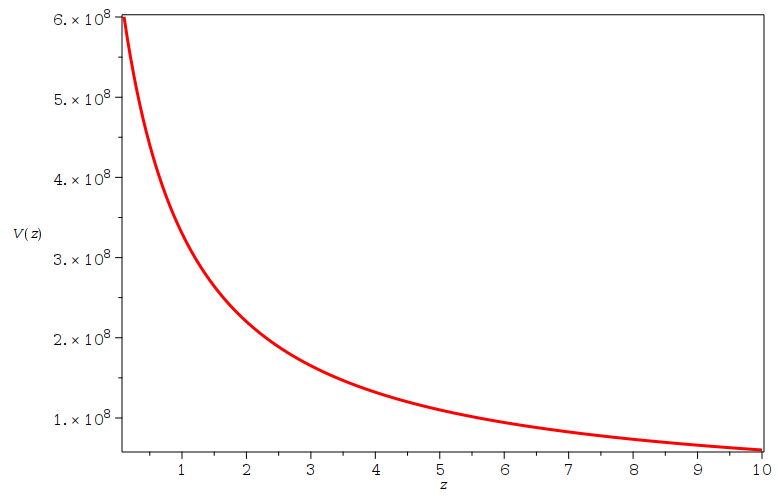
Figure 1: Plot of velocity perturbations versus redshift for $\Lambda$CDM limits, Eq. 91. Normalization was made by multiplying $10^{2}$ to the $V(z)$.

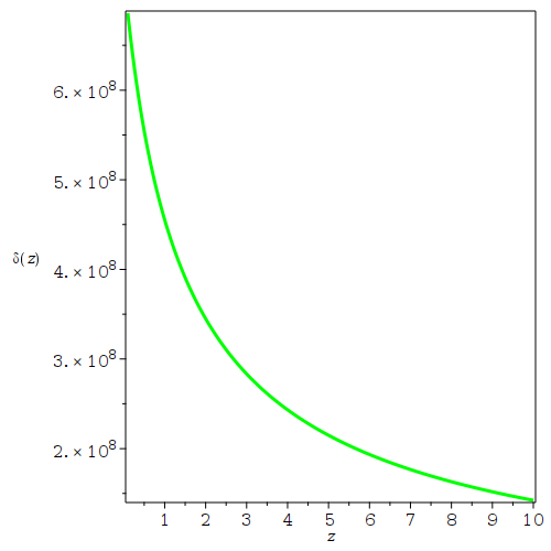
Figure 2: Plot of energy density perturbations versus redshift for $\Lambda$CDM limits, Eq. 90. Normalization was made by multiplying $10^{2}$ to the $\delta(z)$.

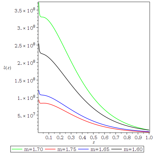
Figure 3: Plot of energy density perturbations versus redshift of Eq. 87-89 for different values of $m$ with $k\ll 1$. To find numerical results, we considered the relation $\frac{k^{2}}{a^{2}H^{2}}=\frac{16\pi^{2}}{\lambda^{2}(1+z)^{2}}$ throughout all plots.

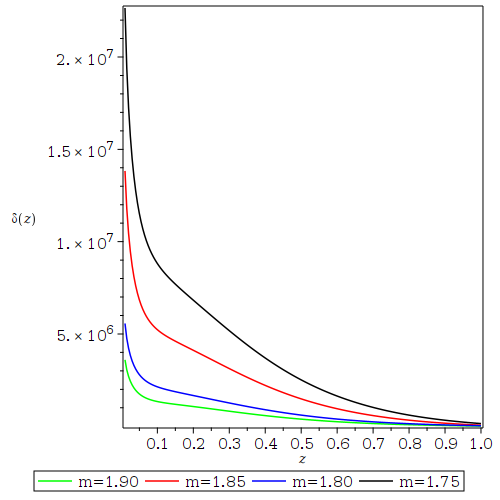
Figure 4: Plot of energy density perturbations versus redshift of Eq. 87-89 for different values of $m$ with $k\gg 1$.

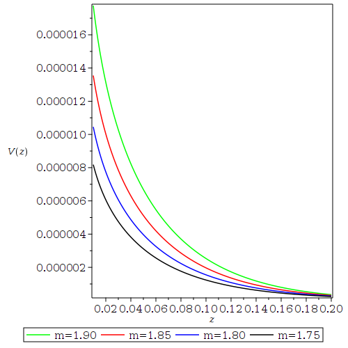
Figure 5: Plot of velocity perturbations versus redshift of Eq. 87-89 for different values of $m$ with $k\ll 1$.

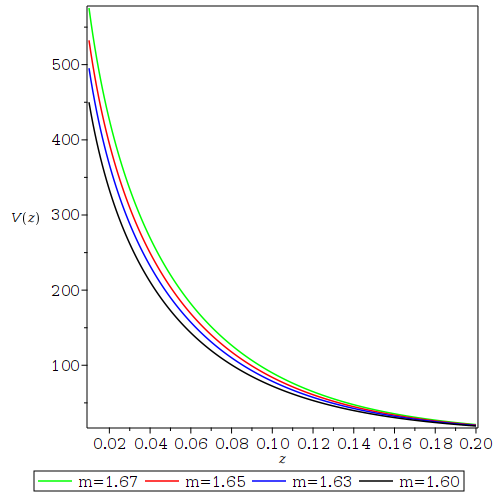
Figure 6: Plot of velocity perturbations versus redshift of Eq. 87-89 for different values of $m$ with $k\gg 1$.

We analysed the behavior of velocity and the energy density contrast for different values of $m$. For Velocity perturbations, $V(z)$, the range of the parameter $m$ which presented good results is for $1.75\leq m\leq 1.90$ for long wavelength modes and $1.60\leq m\leq 1.70$ for short wavelength modes.
For the energy density contrast $\delta(z)$, we considered $1.60\leq m\leq 1.70$ for long wavelength modes and $1.75\leq m\leq 1.90$ for short wavelength modes. From all considered ranges of $m$, both energy density contrast and velocity perturbations decay with increase in redshift. The decay of energy density contrast seems to be non linear compared with the $\Lambda$CDM limits.
For the velocity perturbations, the decay mimics the $\Lambda$CDM limits, only differs for higher amplitudes. For both the energy density contrast and velocity perturbations, the numerical results present higher amplitudes for short wavelength than for long wavelength modes.

4.5 Quasi-static aproximation

For small scale perturbations, perturbations due to Gauss-Bonnet contributions will slowly evolve compared to the matter energy density perturbations[50, 71, 16, 17] therefore, we use a Quasi-static approximation, where the temporal derivatives in the Gauss-Bonnet term $G$ are neglected it means $\ddot{\mathcal{G}}\approx 0$ and $\dot{\mathcal{G}}\approx 0$. Therefore the overall dynamics of the density and velocity perturbations of the system of equations Eq. (82)-(84) after redshift transformation can be presented as

$$\Delta^{\prime\prime}_{m}-\frac{1}{(1+z)}\left(\frac{1}{2}+\mathcal{Y}\right)\Delta^{\prime}_{m}-\frac{3\Omega_{m}}{2(1+z)^{2}}\Delta_{m}$$

$$\quad\quad+\frac{1}{1+z}\left[\frac{\beta}{H\gamma}\left[\dot{G}\left(\dot{G}\varepsilon+\frac{G\mathcal{Y}}{36H^{2}}-\frac{1}{3}\right)-2\ddot{G}\right]+3H\left(-1-\Omega_{m}+2\mathcal{X}\right)-3\mu\right]V^{\prime}_{m}$$

$$\quad\quad-\frac{1}{(1+z)^{2}}\left[3\Omega_{m}\left(-\frac{\beta}{2\gamma}\left(1+\frac{\mathcal{Y}}{8H\theta^{2}}\right)\dot{G}+\frac{3}{2}H+\frac{G\mathcal{Y}}{48H^{2}}\right)-\frac{\mathcal{Y}}{H}\frac{k^{2}}{a^{2}}\right]V_{m}=0\;,$$ (96)

$$V^{\prime\prime}_{m}+\frac{1}{(1+z)}\left(\frac{1}{2}-\nu-\frac{\eta}{H\gamma}\dot{G}\left(\dot{G}\varepsilon+\frac{G\mathcal{Y}}{36H^{2}}-\frac{1}{3}\right)-2\ddot{G}\right)V^{\prime}_{m}$$

$$\quad\quad-\frac{3\Omega_{m}}{2(1+z)^{2}}\left[\left(1+\frac{\mathcal{Y}}{8H\theta^{2}}\right)\left(1-\frac{\eta}{\gamma}\right)\right]V_{m}=0\;.$$ (97)

From Eq. 96, energy density couple with velocity perturbations while from Eq. 97 energy density perturbations decouple from velocity perturbations. Numerical solutions of Eq. 96 and Eq. 97 are presented in Fig. 9-9.

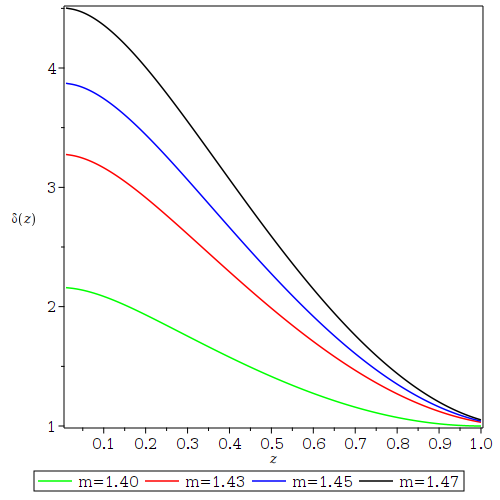
Figure 7: Plot of energy density perturbations versus redshift of Eq. 96-97 for different values of $m$ with $k\ll 1$.

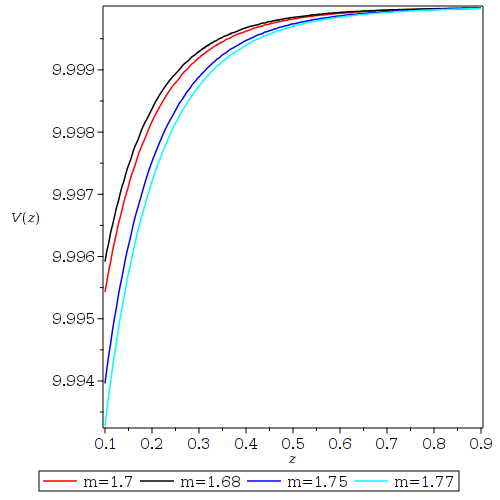
Figure 8: Plot of velocity perturbations versus redshift of Eq. 96-97 for different values of $m$ with $k\ll 1$.

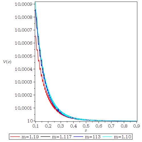
Figure 9: Plot of velocity perturbations versus redshift of Eq. 96-97 for different values of $m$ with $k\ll 1$.

In order to get the numerical results of Eq. 96 and Eq. 97 simultaneously, we set different values of the parameter $m$, the consideration of the initial conditions and the normalization. The numerical solutions for both energy density contrast and velocity perturbations were only evaluated for long wavelength modes. For $1.40\leq m\leq 1.47$, energy density contrast decays with increasing redshift as presented in fig. 9. For $1.10\leq m\leq 1.19$, the velocity perturbations decay with increase in redshift as presented in fig. 9, which is not the case for the consideration of $1.68\leq m\leq 1.77$ as presented in fig. 9. We depict unrealistic behavior of the velocity perturbations. For both the energy density contrast and the velocity perturbations, the $\Lambda$CDM limit is recovered for the case $f(G)=G$ or $m=1$.

5 Discussion and Conclusion

In this paper, we have considered a specific $f(G)$ gravity model which provides the expansion history of the Universe for a power-law cosmological scale factor which can mimic the $\Lambda CDM$ model. The considered non-linear $f(G)$ model has been studied to be able to drive the inflationary era in the early epoch and can describe the late time cosmic acceleration. For example, in Capozziello et al [35], the considered $f(R,G)$ model with both $R$ and $G$ treated to be non-linear. This paper presents a detailed analysis of the $1+3$ covariant velocity and energy density perturbations of the quasi-newtonian cosmology in the context of $f(G)$ gravity. From propagation and constraints equations, we have derived first and second integrability conditions for $f(G)$ gravity, where we were able to obtain covariant velocity, acceleration and the modified Poisson equations for both $f(G)$ gravity and $\Lambda$CDM model. The obtained velocity and acceleration equations were coupled then decoupled to a second order differential equations. Since our interest extends to the large-scale structure formation, we have derived scalar velocity and energy density perturbation equations. In doing so, we have defined gauge invariant scalar gradient variables and derived their corresponding scalar linear evolution equations. We then apply harmonic decomposition method together with the redshift transformation technique to make equations manageable for analysis. From that, we solve the whole system of equations without considering the quasi-static approximation. We obtain both of the analytical and numerical solutions for both velocity and matter energy density for $\Lambda$CDM limits while numerical results were obtained for the considered $f(G)$ model. We computed the growth of fractional energy density $\delta(z)$ and velocity $\mathcal{V}(z)$ for the considered $f(G)$ model and the power-law cosmological scale factor. From the plots, We depict that both $\delta(z)$ and $V(z)$ decay with redshift for long and short wavelength modes. For the case $m=1$, this decay of $\delta(z)$ and $V(z)$ with redshift presents a feature mimicking the $\Lambda$CDM limits.

On the other hand, we have considered the quasi-static approximation for analysing small scale perturbations where temporal derivatives of the Gauss-Bonnet fluid energy density and momentum were discarded. We show that $\delta(z)$ and $\mathcal{V}(z)$ decay with redshift for the considered range of parameter $m$.

Some of the specific highlights of the present paper include:

• We have presented the integrability conditions, covariant modified Poisson equation in $f(G)$ gravity, evolution of velocity and $4$-acceleration in modified $f(G)$ gravity in Eq. 55, Eq. 57,Eq. 60, Eq. 63,Eq. 65, and energy density and velocity perturbations Eq. 87 through to Eq. 89in quasi-newtonian space-time in $f(G)$ gravity which can be reduced to GR limits for the case of linear $f(G)$ gravity.

• During the analysis stage, we have considered short and long wavelength modes for the perturbation equations in a dust-Gauss-Bonnet fluids and considered a combination of non-linear $f(G)$ models with a linear $f(R)$ model such that, for the case $f(G)$ is choosen to be linear ($f(G)=G$), we recover GR limits.

• The numerical results of the velocity and energy density perturbations are presented in figures Fig. 2- 9 for both short and long wavelength modes. From the plots, for a linear $f(G)$ case, we depict the contribution of dust fluid in quasi-newtonian spacetime universe for matter energy density and velocity perturbations which decay with increasing redshift.

• We presented the range of parameter $m$ for which both the energy density and velocity perturabtions decay with increase in redshift [76, 12, 68].

• The current results show that for both energy density and velocity perturbations, the quasi-newtonian spacetime in modified $f(G)$ gravity offers an alternative for large scale structure formation since the energy density and velocity perturbations decay with redshift hence can provide a room in the understanding of cosmic acceleration scenario.

In Quasi-Newtonian space-time without considering the quasi-static approximation, both energy density and velocity perturbations couple with the perturbations due to the Gauss-Bonnet contributions whereas by considering the quasi-static approximations, Both energy density and velocity perturbations decouple from the perturbations due to the Gauss-Bonnet contribution. By refering to the numerical results, the quasi-static approximation is not applicable for short-wavelength modes and for long-wavelength modes as $m$ get large since the velocity perturbations do not decay with redshift for the considered range of parameter $m$. In conclusion, we deduce that the energy density contrast and velocity perturbations decay with redshift for the considered $f(G)$ model without quasi-static approximation for all range of parameter $m$ considered for both long and short wavelength modes. By considering quasi-static approximations, the energy density contrast decay with increase in redshift in long wavelength modes and the velocity perturbations decay with increasing redshift for $m$ getting closer to $1$, but show unrealistic features for large values of parameter $m$ in the long wavelength modes. Both energy density contrast and velocity perturbations results coincide with the $\Lambda$CDM limits for the case $f(G)=G$. The $\delta(z)$ and $\mathcal{V}(z)$ for the considered $f(G)$ model are consistent with the $\Lambda$CDM predictions for the considered range of parameter $m$, therefore the large-scale structure formation is enhanced. The future work should consider different $f(G)$ models to check for the consistency with different observational predictions.

Appendix A Useful Linearised Differential Identities

For all scalars $f$, vectors $V_{a}$ and tensors that vanish in the background, $S_{ab}=S_{\langle ab\rangle}$, the following linearised identities hold:

$$\left(\tilde{\nabla}_{\langle a}\tilde{\nabla}_{b\rangle}f\right)^{.} = \tilde{\nabla}_{\langle a}\tilde{\nabla}_{b\rangle}\dot{f}-{\textstyle{2\over 3}}\Theta\tilde{\nabla}_{\langle a}\tilde{\nabla}_{b\rangle}f+\dot{f}\tilde{\nabla}_{\langle a}A_{b\rangle}\;,$$ (98)

$$\varepsilon^{abc}\tilde{\nabla}_{b}\tilde{\nabla}_{c}f = 0\;,$$ (99)

$$\varepsilon_{cda}\tilde{\nabla}^{c}\tilde{\nabla}_{\langle b}\tilde{\nabla}^{d\rangle}f = \varepsilon_{cda}\tilde{\nabla}^{c}\tilde{\nabla}_{(b}\tilde{\nabla}^{d)}f=\varepsilon_{cda}\tilde{\nabla}^{c}\tilde{\nabla}_{b}\tilde{\nabla}^{d}f=0\;,$$ (100)

$$\tilde{\nabla}^{2}\left(\tilde{\nabla}_{a}f\right) = \tilde{\nabla}_{a}\left(\tilde{\nabla}^{2}f\right)+{\textstyle{1\over 3}}\tilde{R}\tilde{\nabla}_{a}f\;,$$ (101)

$$\left(\tilde{\nabla}_{a}f\right)^{\displaystyle{\cdot}} = \tilde{\nabla}_{a}\dot{f}-{\textstyle{1\over 3}}\Theta\tilde{\nabla}_{a}f+\dot{f}A_{a}\;,$$ (102)

$$\left(\tilde{\nabla}_{a}S_{b\cdots}\right)^{\displaystyle{\cdot}} = \tilde{\nabla}_{a}\dot{S}_{b\cdots}-{\textstyle{1\over 3}}\Theta\tilde{\nabla}_{a}S_{b\cdots}\;,$$ (103)

$$\left(\tilde{\nabla}^{2}f\right)^{\displaystyle{\cdot}} = \tilde{\nabla}^{2}\dot{f}-{\textstyle{2\over 3}}\Theta\tilde{\nabla}^{2}f+\dot{f}\tilde{\nabla}^{a}A_{a}\;,$$ (104)

$$\tilde{\nabla}_{[a}\tilde{\nabla}_{b]}V_{c} = -{\textstyle{1\over 6}}\tilde{R}V_{[a}h_{b]c}\;,$$ (105)

$$\tilde{\nabla}_{[a}\tilde{\nabla}_{b]}S^{cd} = -{\textstyle{1\over 3}}\tilde{R}S_{[a}{}^{(c}h_{b]}{}^{d)}\;,$$ (106)

$$\tilde{\nabla}^{a}\left(\varepsilon_{abc}\tilde{\nabla}^{b}V^{c}\right) = 0\;,$$ (107)

$$\tilde{\nabla}_{b}\left(\varepsilon^{cd\langle a}\tilde{\nabla}_{c}S^{b\rangle}_{d}\right) = {\textstyle{1\over 2}}\varepsilon^{abc}\tilde{\nabla}_{b}\left(\tilde{\nabla}_{d}S^{d}_{c}\right)\;,$$ (108)

$$\text{curlcurl}V_{a} = \tilde{\nabla}_{a}\left(\tilde{\nabla}^{b}V_{b}\right)-\tilde{\nabla}^{2}V_{a}+{\textstyle{1\over 3}}\tilde{R}V_{a}\;,$$ (109)

Appendix B Used equations

For more simplicity, we introduce here some quantities such as:

$$\quad\quad\alpha=(1-G)f^{\prime}-f^{\prime\prime}+\frac{4}{9}\theta^{3}\dot{G}f^{\prime\prime\prime}\;,$$

$$\quad\quad\beta=\frac{\dot{G}}{2}(f^{\prime\prime}+Gf^{\prime\prime\prime})+\theta\left(\dot{G}f^{\prime\prime\prime}-\frac{\theta f^{\prime\prime}}{3}\right)\left(\frac{2}{9}\theta^{2}+\frac{G\dot{G}f^{\prime\prime}}{3}\right)$$

$$\quad\quad-\frac{1}{2}\left((1-G)f^{\prime}-f^{\prime\prime}+\frac{4}{9}\theta^{3}\dot{G}f^{\prime\prime\prime}\right)\;,$$

$$\quad\quad\gamma=\dot{G}\left(f^{\prime\prime\prime}\dot{G}-\frac{\theta}{3}f^{\prime\prime}\right)\left(\frac{2}{9}\theta^{2}+\frac{G\dot{G}f^{\prime\prime}}{3}\right)+\frac{\dot{G}^{2}}{2\theta}\left(f^{\prime\prime}+Gf^{\prime\prime\prime}\right)+\frac{\dddot{G}}{\dot{G}}\;,$$

$$\quad\quad\eta=\left(f^{\prime\prime\prime}\dot{G}-\frac{\theta}{3}f^{\prime\prime}\right)\left(\frac{2}{9}\theta^{2}+\frac{G\dot{G}f^{\prime\prime}}{3}\right)+\frac{\dot{G}}{2\theta}\left(f^{\prime\prime}+Gf^{\prime\prime\prime}\right)\;,$$

$$\quad\quad\zeta=\frac{1}{3}\theta+\frac{G\dot{G}^{2}(f^{\prime\prime})^{2}}{3}+\frac{2}{9}\dot{G}\theta^{2}f^{\prime\prime}\;,$$

$$\quad\quad\varepsilon=\frac{G\dot{G}(f^{\prime\prime})^{2}}{3}+\frac{2}{9}\theta^{2}f^{\prime\prime}+\frac{Gf^{\prime\prime}}{2\theta}\;,$$

$$\quad\quad\mu=\frac{4}{3}\theta+\frac{4}{9}\theta^{2}\dot{G}f^{\prime\prime}+\frac{1}{3}\dot{G}^{2}f^{\prime\prime 2}-\frac{10}{9}\theta^{2}\dot{G}f^{\prime\prime}\;$$

$$\quad\quad\nu=2H\dot{G}f^{\prime\prime}+\frac{G\dot{G}^{2}(f^{\prime\prime})^{2}}{3H}\;.$$ (110)

We introduce dimensionless variables as:

$$\mathcal{X}=\frac{Gf^{\prime}-f}{6H^{2}}\;,$$

$$\quad\quad\Omega_{m}=\frac{\rho_{m}}{3H^{2}}\;,$$

$$\quad\quad\mathcal{Y}=6H\dot{G}f^{\prime\prime}.$$ (111)

We can present different useful equations in redshift space as

$$\dot{H}=-\frac{2m}{3}(1+z)^{\frac{3}{m}}$$

$$\dot{G}=\frac{256}{9}m^{3}\Big{(}1-\frac{2m}{3}\Big{)}(1+z)^{\frac{15}{2m}}$$

$$\ddot{G}=1280m^{3}\Big{(}\frac{2m}{3}-1\Big{)}(1+z)^{\frac{9}{m}}$$

$$\dddot{G}=\frac{2560}{3}m^{3}\Big{(}1-\frac{2m}{3}\Big{)}(1+z)^{\frac{21}{2m}}.$$ (112)

References

- [1] Saul Perlmutter, G Aldering, M Della Valle, S Deustua, RS Ellis, S Fabbro, A Fruchter, G Goldhaber, DE Groom, IM Hook, et al. Discovery of a supernova explosion at half the age of the universe. Nature, 391(6662):51–54, 1998.
- [2] Adam G Riess, Alexei V Filippenko, Peter Challis, Alejandro Clocchiatti, Alan Diercks, Peter M Garnavich, Ron L Gilliland, Craig J Hogan, Saurabh Jha, Robert P Kirshner, et al. Observational evidence from supernovae for an accelerating universe and a cosmological constant. The Astronomical Journal, 116(3):1009, 1998.
- [3] Guido Cognola, Emilio Elizalde, Shin’ichi Nojiri, Sergei D Odintsov, and Sergio Zerbini. Dark energy in modified gauss-bonnet gravity: Late-time acceleration and the hierarchy problem. Physical Review D, 73(8):084007, 2006.
- [4] David W Hogg, Daniel J Eisenstein, Michael R Blanton, Neta A Bahcall, J Brinkmann, James E Gunn, and Donald P Schneider. Cosmic homogeneity demonstrated with luminous red galaxies. The Astrophysical Journal, 624(1):54, 2005. Dragan Huterer and Michael S Turner. Prospects for probing the dark energy via supernova distance measurements. Physical Review D, 60(8):081301, 1999.
- [5] Alexei V Filippenko and Adam G Riess. Results from the high-z supernova search team. Physics Reports, 307(1-4):31–44, 1998.
- [6] G Hinshaw, MR Nolta, CL Bennett, R Bean, O Doré, MR Greason, M Halpern, RS Hill, N Jarosik, A Kogut, et al. Three-year wilkinson microwave anisotropy probe (wmap*) observations: Temperature analysis. The Astrophysical Journal Supplement Series, 170(2):288, 2007.
- [7] Uroš Seljak, Alexey Makarov, Patrick McDonald, Scott F Anderson, Neta A Bahcall, J Brinkmann, Scott Burles, Renyue Cen, Mamoru Doi, James E Gunn, et al. Cosmological parameter analysis including sdss ly forest and galaxy bias: constraints on the primordial spectrum of fluctuations, neutrino mass, and dark energy. Physical Review D, 71(10):103515, 2005.
- [8] Venikoudis SA, Fasoulakos KV and Fronimos FP Late-time Cosmology of scalar field assisted f (G) gravity. International Journal of Modern Physics D,31(05):2250038,2022.
- [9] Daniel J Eisenstein, Idit Zehavi, David W Hogg, Roman Scoccimarro, Michael R Blanton, Robert C Nichol, Ryan Scranton, Hee-Jong Seo, Max Tegmark, Zheng Zheng, et al. Detection of the baryon acoustic peak in the large-scale correlation function of sdss luminous red galaxies. The Astrophysical Journal, 633(2):560, 2005.
- [10] Bhuvnesh Jain and Andy Taylor. Cross-correlation tomography: measuring dark energy evolution with weak lensing. Physical Review Letters, 91(14):141302, 2003.
- [11] Naureen Goheer, Rituparno Goswami, Peter KS Dunsby, and Kishore Ananda. Coexistence of matter dominated and accelerating solutions in gravity. Physical Review D, 79(12):121301, 2009.
- [12] Amare Abebe, Alvaro de la Cruz-Dombriz, and Peter KS Dunsby. Large scale structure constraints for a class of theories of gravity. Physical review D, 88(4):044050, 2013.
- [13] RT Hough, Amare Abebe, and SES Ferreira. Viability tests of -gravity models with supernovae type 1a data. The European Physical Journal C, 80(8):1–15, 2020.
- [14] Amare Abebe, Rituparno Goswami, and Peter KS Dunsby. Shear-free perturbations of gravity. Physical Review D, 84(12):124027, 2011.
- [15] Heba Sami, Neo Namane, Joseph Ntahompagaze, Maye Elmardi, and Amare Abebe. Reconstructing gravity from a chaplygin scalar field in de sitter spacetimes. International Journal of Geometric Methods in Modern Physics, 15(02):1850027, 2018.
- [16] Shambel Sahlu, Joseph Ntahompagaze, Amare Abebe, Álvaro de la Cruz-Dombriz, and David F Mota. Scalar perturbations in gravity using the 1+ 31+ 3 covariant approach. The European Physical Journal C, 80(5):1–19, 2020.
- [17] Heba Sami, Shambel Sahlu, Amare Abebe, and Peter KS Dunsby. Covariant density and velocity perturbations of the quasi-newtonian cosmological model in gravity. The European Physical Journal C, 81(10):1–17, 2021.
- [18] Shambel Sahlu, Joseph Ntahompagaze, Amare Abebe, and David F Mota. Inflationary constraints in teleparallel gravity theory. International Journal of Geometric Methods in Modern Physics, 18(02):2150027, 2021.
- [19] Shambel Sahlu and Endalkachew Tsegaye. Linear cosmological perturbations in gravity. arXiv preprint arXiv:2206.02517, 2022.
- [20] Laur Järv, Mihkel Rünkla, Margus Saal, and Ott Vilson. Nonmetricity formulation of general relativity and its scalar-tensor extension. Physical Review D, 97(12):124025, 2018.
- [21] Jose Beltrán Jiménez, Lavinia Heisenberg, Tomi Koivisto, and Simon Pekar. Cosmology in geometry. Physical Review D, 101(10):103507, 2020.
- [22] Kai Flathmann and Manuel Hohmann. Parametrized post-newtonian limit of generalized scalar-nonmetricity theories of gravity. Physical Review D, 105(4):044002, 2022.
- [23] Luís Atayde and Noemi Frusciante. Can gravity challenge cdm? Physical Review D, 104(6):064052, 2021.
- [24] Wompherdeiki Khyllep, Andronikos Paliathanasis, and Jibitesh Dutta. Cosmological solutions and growth index of matter perturbations in gravity. Physical Review D, 103(10):103521, 2021.
- [25] Baojiu Li, John D Barrow, and David F Mota. Cosmology of modified gauss-bonnet gravity. Physical Review D, 76(4):044027, 2007.
- [26] AR Rastkar, MR Setare, and F Darabi. Phantom phase power-law solution in gravity. Astrophysics and Space Science, 337(1):487–491, 2012.
- [27] Albert Munyeshyaka, Joseph Ntahompagaze, and Tom Mutabazi. Cosmological perturbations in gravity. International Journal of Modern Physics D, 30(07):2150053, 2021.
- [28] De Felice, Antonio and Tsujikawa, Shinji, Construction of cosmologically viable gravity models Physics Letters B, 675(1): 1–8, 2009.
- [29] Amendola, Luca and Polarski, David and Tsujikawa, Shinji Are f (R) dark energy models cosmologically viable? Physical review letters, 98(13): 131302, 2007.
- [30]
- [31] Salvatore Capozziello. Curvature quintessence. International Journal of Modern Physics D, 11(04):483–491, 2002.
- [32] Nicholas David Birrell, Nicholas David Birrell, and PCW Davies. Quantum fields in curved space. 1984.
- [33] NH Barth and SM Christensen. Quantizing fourth-order gravity theories: the functional integral. Physical Review D, 28(8):1876, 1983.
- [34] Antonio De Felice and Takahiro Tanaka. Inevitable ghost and the degrees of freedom in gravity. Progress of Theoretical Physics, 124(3):503–515, 2010.
- [35] Salvatore Capozziello, Mariafelicia De Laurentis, and Sergei D Odintsov. Noether symmetry approach in gauss–bonnet cosmology. Modern Physics Letters A, 29(30):1450164, 2014.
- [36] Mariafelicia De Laurentis, Mariacristina Paolella, and Salvatore Capozziello. Cosmological inflation in gravity. Physical Review D, 91(8):083531, 2015.
- [37] Micol Benetti, Simony Santos da Costa, Salvatore Capozziello, Jailson S Alcaniz, and Mariafelicia De Laurentis. Observational constraints on gauss–bonnet cosmology. International Journal of Modern Physics D, 27(08):1850084, 2018.
- [38] Shin’ichi Nojiri, Sergei D Odintsov, Alexey Toporensky, and Petr Tretyakov. Reconstruction and deceleration–acceleration transitions in modified gravity. General Relativity and Gravitation, 42(8):1997–2008, 2010.
- [39] Guido Cognola, Emilio Elizalde, Shin’ichi Nojiri, Sergei D Odintsov, and Sergio Zerbini. String-inspired gauss-bonnet gravity reconstructed from the universe expansion history and yielding the transition from matter dominance to dark energy. Physical Review D, 75(8):086002, 2007.
- [40] Shin’ichi Nojiri, Sergei D Odintsov, and M Sami. Dark energy cosmology from higher-order, string-inspired gravity, and its reconstruction. Physical Review D, 74(4):046004, 2006.
- [41] Álvaro De la Cruz-Dombriz and Diego Sáez-Gómez. On the stability of the cosmological solutions in gravity. Classical and Quantum Gravity, 29(24):245014, 2012.
- [42] LN Granda. Natural scaling for dark energy. Modern Physics Letters A, 28(28):1350117, 2013.
- [43] Yong-Seon Song, Wayne Hu, and Ignacy Sawicki. Large scale structure of gravity. Physical Review D, 75(4):044004, 2007.
- [44] Antonio De Felice, Jean-Marc Gerard, and Teruaki Suyama. Cosmological perturbation in theories with a perfect fluid. Physical Review D, 82(6):063526, 2010.
- [45] James M Bardeen. Gauge-invariant cosmological perturbations. Physical Review D, 22(8):1882, 1980.
- [46] Hideo Kodama and Misao Sasaki. Cosmological perturbation theory. Progress of Theoretical Physics Supplement, 78:1–166, 1984.
- [47] Peter KS Dunsby. Gauge invariant perturbations in multi-component fluid cosmologies. Classical and Quantum Gravity, 8(10):1785, 1991.
- [48] Peter KS Dunsby, Marco Bruni, and George FR Ellis. Covariant perturbations in a multifluid cosmological medium. The Astrophysical Journal, 395:54–74, 1992.
- [49] George FR Ellis and Marco Bruni. Covariant and gauge-invariant approach to cosmological density fluctuations. Physical Review D, 40(6):1804, 1989.
- [50] Amare Abebe, Mohamed Abdelwahab, Álvaro De la Cruz-Dombriz, and Peter KS Dunsby. Covariant gauge-invariant perturbations in multifluid gravity. Classical and quantum gravity, 29(13):135011, 2012.
- [51] Joseph Ntahompagaze, Amare Abebe, and Manasse Mbonye. On gravity in scalar–tensor theories. International Journal of Geometric Methods in Modern Physics, 14(07):1750107, 2017.
- [52] Joseph Ntahompagaze, Shambel Sahlu, Amare Abebe, and Manasse R Mbonye. On multifluid perturbations in scalar–tensor cosmology. International Journal of Modern Physics D, 29(16):2050120, 2020.
- [53] Joseph Ntahompagaze, Amare Abebe, and Manasse Mbonye. A study of perturbations in scalar–tensor theory using 1+ 3 covariant approach. International Journal of Modern Physics D, 27(03):1850033, 2018.
- [54] Chris A Clarkson and Richard K Barrett. Covariant perturbations of schwarzschild black holes. Classical and Quantum Gravity, 20(18):3855, 2003.
- [55] Maye Elmardi, Amare Abebe, and Abiy Tekola. Chaplygin-gas solutions of gravity. International Journal of Geometric Methods in Modern Physics, 13(10):1650120, 2016.
- [56] Henk Van Elst, Claes Uggla, William M Lesame, George FR Ellis, and Roy Maartens. Integrability of irrotational silent cosmological models. Classical and Quantum Gravity, 14(5):1151, 1997.
- [57] Roy Maartens. Covariant velocity and density perturbations in quasi-newtonian cosmologies. Physical Review D, 58(12):124006, 1998.
- [58] Henk Van Elst and George FR Ellis. Quasi-newtonian dust cosmologies. Classical and Quantum Gravity, 15(11):3545, 1998.
- [59] Heba Sami and Amare Abebe. Quasi-newtonian scalar-tensor cosmologies.
- [60] Aghanim Nabila, Akrami Yashar, Ashdown Mark, Aumont J, Baccigalupi C, Ballardini M, Banday AJ, Barreiro RB, Bartolo N, Basak S and others. Planck 2018 results-VI. Cosmological parameters. Astronomy & Astrophysics, 641,A6,2020.
- [61] Heba Sami and Amare Abebe. Perturbations of quasi-newtonian universes in scalar–tensor gravity. International Journal of Geometric Methods in Modern Physics, 18(10):2150158, 2021.
- [62] Roy Maartens, William M Lesame, and George FR Ellis. Newtonian-like and anti-newtonian universes. Classical and Quantum Gravity, 15(4):1005, 1998.
- [63] MAH MacCallum. ” integrability in tetrad formalisms and conservation in cosmology. In Proceedings of the International Seminar Current Topics in Mathematical Cosmology: Potsdam, Germany, volume 30, page 133. World Scientific, 1998.
- [64] Roy Maartens, William M Lesame, and George FR Ellis. Consistency of dust solutions with div h= 0. Physical Review D, 55(8):5219, 1997.
- [65] Gourgoulhon, Eric. 3+ 1 formalism and bases of numerical relativity. arXiv preprint gr-qc/0703035, 2007.
- [66] Park, Chan. A Covariant Approach to 1+ 3 Formalism. arXiv preprint arXiv:1810.06293, 2018
- [67] Kotub Uddin, James E Lidsey, and Reza Tavakol. Cosmological scaling solutions in generalised gauss–bonnet gravity theories. General Relativity and Gravitation, 41(12):2725–2736, 2009.
- [68] Albert Munyeshyaka, Abraham Ayirwanda, Fidele Twagirayezu, Beatrice Murorunkwere, and Joseph Ntahompagaze. Multifluid cosmology in gravity. International Journal of Geometric Methods in Modern Physics, 2022.
- [69] George FR Ellis. Republication of: Relativistic cosmology. General Relativity and Gravitation, 41(3):581–660, 2009.
- [70] Nadiezhda Montelongo Garcia, Tiberiu Harko, Francisco SN Lobo, and José P Mimoso. Energy conditions in modified gauss-bonnet gravity. Physical Review D, 83(10):104032, 2011.
- [71] Amare Abebe, Peter KS Dunsby, and Deon Solomons. Integrability conditions of quasi-newtonian cosmologies in modified gravity. International Journal of Modern Physics D, 26(06):1750054, 2017.
- [72] Amare Abebe and Maye Elmardi. Irrotational-fluid cosmologies in fourth-order gravity. International Journal of Geometric Methods in Modern Physics, 12(10):1550118, 2015.
- [73] Amare Abebe. Breaking the cosmological background degeneracy by two-fluid perturbations in gravity. International Journal of Modern Physics D, 24(07):1550053, 2015.
- [74] Sante Carloni, Peter KS Dunsby, and Claudio Rubano. Gauge invariant perturbations of scalar-tensor cosmologies: The vacuum case. Physical Review D, 74(12):123513, 2006.
- [75] Beatrice Murorunkwere, Joseph Ntahompagaze, and Edward Jurua. 1+ 3 covariant perturbations in power-law gravity. The European Physical Journal C, 81(4):1–10, 2021.
- [76] Kishore N Ananda, Sante Carloni, and Peter KS Dunsby. Structure growth in theories of gravity with a dust equation of state. Classical and Quantum Gravity, 26(23):235018, 2009.