Reconstructing black hole exteriors and interiors using entanglement and complexity

Abstract

Based on the AdS/CFT correspondence, we study how to reconstruct bulk spacetime metrics by various quantum information measures on the boundary field theories, which include entanglement entropy, mutual information, entanglement of purification, and computational complexity according to the proposals of complexity=volume 2.0 and complexity=generalized volume. We present several reconstruction methods, all of which are free of UV divergence and most of which are driven by the derivatives of the measures with respect to the boundary scales. We illustrate that the exterior and interior of a black hole can be reconstructed using the measures of spatial entanglement and time-evolved complexity, respectively. We find that these measures always probe the spacetime in a local way: reconstructing the bulk metric in different radial positions requires the information at different boundary scales. We also show that the reconstruction method using complexity=volume 2.0 is the simplest and has a certain strong locality.

1 Introduction

Anti-de Sitter/conformal field theory (AdS/CFT) correspondence not only provides a gravitational lens for strongly coupled quantum field theories but also brings a wealth of insights for quantum gravity Maldacena:1997re ; Gubser:1998bc ; Witten:1998qj ; Liu:2020rrn ; Susskind:1998dq . The essential challenge in exploring this correspondence is to understand how the boundary degrees of freedom of the CFT can be reorganized under certain limits into the local gravitational physics in the bulk. This ambitious program is widely termed as ‘bulk reconstruction’.

Bulk reconstruction is a non-trivial inverse problem that involves holographic mapping from low to high dimensions. One of the most fascinating branches in this program is the reconstruction of the metric of the holographic spacetime. There are various methods regarding the bulk metric reconstruction, which use different boundary physical quantities, such as the source and expectation value of energy-momentum tensor deHaro:2000vlm , the singularities in the set of correlation functions Hammersley:2006cp ; Hubeny:2006yu , the entanglement entropy (EE) of boundary intervals Hammersley:2007ab ; Hubeny:2012ry ; Bilson:2008ab ; Bilson:2010ff , the differential entropy that is a UV-finite combination of EE Balasubramanian:2013lsa ; Myers:2014jia ; Czech:2014ppa , the divergence structure of boundary $n$-point function Engelhardt:2016wgb ; Engelhardt:2016crc , the modular Hamiltonians of boundary subregions Roy:2018ehv ; Kabat:2018smf , the Wilson loops related to quark potential Hashimoto:2020mrx , and four-point correlators in an excited quantum state Caron-Huot2211 , among others. It is worth noting that much of the work on metric reconstruction has been driven by the idea that spacetime is built by quantum entanglement Takayanagi T ; Maldacena:2001kr ; Ryu:2006bv ; Swingle:2009bg ; VanRaamsdonk:2010pw ; Maldacena:2013xja . However, it has been pointed out that ‘entanglement is not enough’ to encode the full spacetime Susskind:2014moa . In order to understand the interior of a black hole, it has been proposed that the quantum computational complexity would be important. In fact, based on the ‘complexity=volume’ (CV) proposal Susskind:2014rva ; Susskind:2014moa , Hashimoto and Watanabe have successfully reconstructed the metric inside black holes Hashimoto:2021umd .

One common challenge in computing physical quantities in quantum field theories is how to address the issue of UV divergence. In the AdS/CFT correspondence, there are systematic methods to cancel the divergence based on the UV/IR connection Susskind:1998dq , which are well known as holographic renormalization Skenderis0209 ; Papadimitriou2016 . However, most of work on holographic renormalization is constrained to the standard AdS/CFT, which requires the conformal symmetry, infinite coupling, and large N limit. How to remove the divergence on gravity and field theory consistently beyond these constraints remains an open question. In light of this, ref. Jokela:2020auu uses the derivative of EE with respect to the spatial size of entangling region $l$ as data, which are insensitive to the UV cutoff, unlike to EE itself. As a result, the reconstruction of metric is free of UV divergence. Note that canceling off the UV divergence has also been a guide to the correct formula for the differential entropy Balasubramanian:2013lsa .

On the other hand, deep learning (DL) algorithms have been utilized to reconstruct the metric Hashimoto:2018ftp ; Hashimoto:2018bnb ; Tan:2019czc ; Akutagawa:2020yeo ; Hashimoto:2020jug ; Yan:2020wcd ; Hashimoto:2019bih ; Hashimoto:2021ihd ; Katsube:2022ofz ; Hashimoto:2022eij ; Li:2022zjc . This not only unlocks the potential for building a data-driven holographic model but also provides insights into holography using the language of machine learning. In ref. Yan:2020wcd , an interesting difference was observed between the analytical reconstruction method using the $l$-dependent EE as data Bilson:2010ff and the DL method using the frequency-dependent shear viscosity: the former ‘locally’ probes the bulk spacetime, while the latter is ‘non-local’. Here the non-local aspect is manifested through the excellent generalization capability of the deep neural network, which enable a narrow frequency to generate a wide frequency shear viscosity, using the learned complete metric as a hidden structure. Conversely, the local aspect indicates that the deeper spacetime is probed through the EE with a larger entangling region.

In this paper, we will explore the reconstruction of bulk metric using various quantum information measures on the boundary field theories. In addition to revisiting EE, we will study mutual information (MI) Wolf:2007tdq and entanglement of purification (EoP) Terhal2002 , both of which are closely related to EE, as well as two candidate measures of complexity that differ from the CV proposal Couch:2016exn ; Belin:2021bga . For most of them, we will use their derivatives with respect to boundary scales as data. Moreover, we will compare how these measures encode the bulk metric. In particular, we will examine whether they always probe the spacetime in a local way.

2 Exterior of black holes

2.1 Entanglement Entropy

As a warm-up, we review the analytical reconstruction method using EE which was proposed by Bilson Bilson:2010ff . The relevant holographic dictionary is the Ryu-Takayanagi formula Ryu:2006bv , by which the EE of the entangling region $A$ on the boundary can be calculated in the bulk spacetime:

$$S=\frac{Area(\gamma_{A})}{4G_{N}}.$$ (1)

Here $G_{N}$ is Newton’s constant and $\gamma_{A}$ is the minimal surface which extends into the bulk and shares the boundary with $\partial A$. Afterwards, we will set $G_{N}=1$ for convenience.

2.1.1 Holographic calculation

We will study a $d+1$-dimensional asymptotically AdS spacetime. As a proof of principle, we focus on a highly symmetric metric ansatz

$$ds^{2}=\frac{1}{z^{2}}\left(-f(z)dt^{2}+\frac{1}{f(z)}dz^{2}+d\vec{x}^{2}\right).\,$$ (2)

We set the planar horizon and boundary located at $z=1$ and $z=0$, respectively. On the boundary, we are interested in a spatial strip entangling region with a width $l$ in one direction and an infinite length $L$ in every other direction. The entangling region and minimal surface are depicted in figure 1.

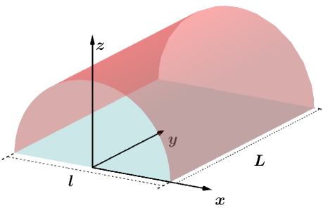
Figure 1: A minimal surface (red) in the bulk and a strip entangling region (blue) on the boundary. EE is given by the area of the red surface.

The area of the minimal surface is a function of $l$, which can be written as

$$A(l)=2L^{d-2}\int_{0}^{\frac{l}{2}}\frac{1}{z^{d-1}}\sqrt{1+\frac{z^{\prime 2}}{f(z)}}dx,$$ (3)

where $z^{\prime}=dz/dx$. The profile of the minimal surface can be obtained as follows. Treating $A(l)$ as an action and $z(x)$ as a generalized coordinate, one can read the Lagrangian

$$\mathcal{L}(z,z^{\prime})=\frac{1}{z^{d-1}}\sqrt{1+\frac{z^{\prime 2}}{f(z)}}.$$ (4)

It leads to the Hamiltonian

$$\mathcal{H}(z,z^{\prime})=z^{\prime}\frac{d\mathcal{L}}{dz^{\prime}}-\mathcal{L}=-\frac{z^{1-d}}{\sqrt{1+\frac{z^{\prime 2}}{f(z)}}}.\,$$ (5)

Since $\mathcal{L}$ does not depend on the variable $x$ explicitly, one can set $\mathcal{H}$ as a constant

$$\mathcal{H}=-z_{\ast}^{1-d},$$ (6)

where $z_{\ast}$ is given by $\left.z^{\prime}\right|_{z=z_{\ast}}=0$. This yields

$$\frac{dz}{dx}=\pm\frac{\sqrt{f(z)(z_{\ast}^{2d-2}-z^{2d-2})}}{z^{d-1}}.$$ (7)

Equation (7) with the boundary conditions $z(\pm l/2)=0$ determines the profile function $z(x)$ for the minimal surface.

From (1), (3) and (7), we have

$$S(z_{\ast}) = \frac{L^{d-2}}{2}\int_{\delta}^{z_{\ast}}\frac{z_{\ast}^{d-1}}{z^{d-1}\sqrt{f(z)}\sqrt{z_{\ast}^{2d-2}-z^{2d-2}}}dz,$$ (8)

$$\,l(z_{\ast}) = 2\int_{0}^{z_{\ast}}\frac{z^{d-1}}{\sqrt{f(z)}\sqrt{z_{\ast}^{2d-2}-z^{2d-2}}}dz,$$ (9)

where $\delta$ is the UV cutoff. Note that when $\delta\rightarrow 0$, EE is divergent. In order to cancel $z_{\ast}$ in two equations above, we take derivatives:

$$\frac{dS(z_{\ast})}{dz_{\ast}}=\frac{L^{d-2}}{2}\left[\frac{1}{\sqrt{f(z_{\ast})}}\lim_{z\rightarrow z_{\ast}}\frac{1}{\sqrt{z_{\ast}^{2d-2}-z^{2d-2}}}-\int_{0}^{z_{\ast}}\frac{(d-1)z^{d-1}z_{\ast}^{d-2}dz}{(z_{\ast}^{2d-2}-z^{2d-2})^{\frac{3}{2}}\sqrt{f(z)}}\right],$$ (10)

$$\frac{dl(z_{\ast})}{dz_{\ast}}=2z_{\ast}^{d-1}\left[\frac{1}{\sqrt{f(z_{\ast})}}\lim_{z\rightarrow z_{\ast}}\frac{1}{\sqrt{z_{\ast}^{2d-2}-z^{2d-2}}}-\int_{0}^{z_{\ast}}\frac{(d-1)z^{d-1}z_{\ast}^{d-2}dz}{(z_{\ast}^{2d-2}-z^{2d-2})^{\frac{3}{2}}\sqrt{f(z)}}\right].$$ (11)

Using the chain rule

$$\frac{dS(l)}{dl}=\frac{dz_{\ast}}{dl}\frac{dS(z_{\ast})}{dz_{\ast}},$$ (12)

one can find

$$\frac{dS(l)}{dl}=\frac{L^{d-2}}{4z_{\ast}^{d-1}}.$$ (13)

This equation builds a relation between $l$ and $z_{\ast}$.

2.1.2 Reconstruction method

The key step of Bilson’s method is to solve an integral equation analytically. Referring to the handbook of integral equations Poly , one can read:

$$f(x) =\int_{a}^{x}\frac{y(t)dt}{\sqrt{g(x)-g(t)}},\,g^{\prime}(x)>0$$

Solution $$\text{{: }}\,y(x)=\frac{1}{\pi}\frac{d}{dx}\int_{a}^{x}dt\frac{f(t)g^{\prime}(t)}{\sqrt{g(x)-g(t)}}.$$ (14)

Applying eq. (14) to eq. (8), one can find

$$\frac{1}{\sqrt{f(z)}}=\frac{4\left(d-1\right)z^{d-1}}{\pi L^{d-2}}\frac{d}{dz}\int_{\delta}^{z}\frac{S(z_{\ast})z_{\ast}^{d-2}}{\sqrt{z^{2d-2}-z_{\ast}^{2d-2}}}dz_{\ast}.$$ (15)

This is the reconstruction formula provided by Bilson Bilson:2010ff . Here $S(z_{\ast})$ is generated by the data $S(l)$ and $l$ is related to $z_{\ast}$ through eq. (13).

The analytic formula (15) is simple. However, the field theory data it inputs is $S(l)$, which is sensitive to the UV cutoff. Following ref. Jokela:2020auu , we will use the derivative $S^{\prime}(l)$ as the data, which is insensitive to the UV cutoff. We apply eq. (14) to eq. (9) instead of eq. (8), which yields a slightly different reconstruction formula

$$\frac{1}{\sqrt{f(z)}}=\frac{d-1}{\pi z^{d-1}}\frac{d}{dz}\int_{0}^{z}\frac{l(z_{\ast})z_{\ast}^{2d-3}}{\sqrt{z^{2d-2}-z_{\ast}^{2d-2}}}dz_{\ast}.$$ (16)

2.1.3 Example

We can check the validity of the reconstruction formula (16) with a simple example. We choose the AdS black hole with $d=2$ and the function $f(z)=1-z^{2}$ as our target metric. Referring to the result of Fischler:2012uv , the EE of a strip of width $l$ is given by

$$S(l)=\frac{1}{2}\log\left[\frac{2}{\delta}\sinh\left(\frac{l}{2}\right)\right].$$ (17)

In our task of bulk reconstruction, the metric is unknown but we are supposed to know

$$S^{\prime}(l)=\frac{1}{4}\coth(\frac{l}{2}).$$ (18)

Combining the data with (13), we find

$$l(z_{\ast})=2\,\text{arctanh}(z_{\ast}).$$ (19)

This formula indicates that when $l$ increases, the top of the geodesic probes the deeper spacetime near the horizon. We visualize the probing way in figure 2. At last, substituting (19) into (16) with $d=2$, we recover our target metric analytically

$$f(z)=1-z^{2}.$$ (20)

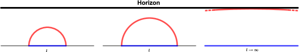
Figure 2: The geodesic probes the deeper spacetime as $l$ increases. As $l$ tends to infinity, the geodesic will approach the horizon.

2.2 Mutual Information

MI is a closely related to EE. It measures the total (both classical and quantum) correlations between two spatial subregions and acts as an upper bound of the connected correlation functions in those regions Wolf:2007tdq ; Swingle:2010jz . The definition of MI between two disjoint subsystems $A$ and $B$ is given by

$$I(A,B)=S_{A}+S_{B}-S_{A\cup B},$$ (21)

where $S_{A}$, $S_{B}$ and $S_{A\cup B}$ denote the EE of the region $A,B$ and ${A\cup B}$ respectively with the rest of the system Fischler:2012uv . Note that EE is a divergent quantity, but MI is finite since three divergent parts in eq. (21) that depend on the UV cutoff cancel out.

2.2.1 Holographic calculation

Consider two disjoint subsystems with strip regions $A$ and $B$, each with width $l$ and length $L\rightarrow\infty$. The interval between them is $a$. For the sake of simplicity, we focus on the symmetric configuration, see figure 3. In this case, $S_{A\cup B}=\min\left[2S(l),S(2l+a)+S(a)\right]$. Depending on the ratio $a/l$, the MI can be written as

$$I(l)=\begin{cases}2S(l)-S(2l+a)-S(a)\,\,\,\,\text{for small ratio $a/l$},\\ \,\,\,\,\,\,\,\,\,\,\,\,0\,\,\,\,\,\,\,\,\,\,\,\,\,\,\,\,\,\,\,\,\,\,\,\,\,\,\,\,\,\,\,\,\,\,\text{for large ratio $a/l$}.\end{cases}$$ (22)

For convenience, we will fix $a$ and change $l$. This induces a critical width $l_{a}$ below which the MI is zero. Note that one cannot reconstruct anything from the region where MI is zero. In fact, we have not found a way to reconstruct the metric through the MI alone.

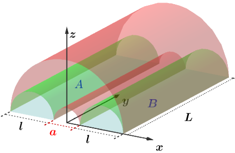
Figure 3: The minimal surfaces (red and green) and two disjoint strip entangling regions (blue) in the symmetric configuration. The nonzero MI is given by the difference between the area of green surfaces and red surfaces.

2.2.2 Reconstruction method

Here we will propose a method which reconstructs the metric by jointly using EE and MI. Suppose that the field theory data we have are the derivatives of MI and EE with different ranges of $l$,

$$I^{\prime}(l),\;l>l_{a}\text{ and }S^{\prime}(l),\;l\leq 2l_{a}+a,$$ (23)

where $a$ (then $l_{a}$) is fixed. A simple but important observation is that one can combine eq. (22) and the data (23) to iteratively generate $S^{\prime}(l)$ with any $l$. The iterative equation can be written as

$$S^{\prime}\left(Q\right)=\left\{\begin{array}[]{c}\;\;S^{\prime}(Q),\;\;\;\;\;\;\;\;\;\;\;\;\;\;\ Q\leq Q_{a}\\ S^{\prime}\left(\frac{Q-a}{2}\right)-\frac{1}{2}I^{\prime}\left(\frac{Q-a}{2}\right),\ Q_{a}<Q\leq 2Q_{a}+a\end{array}\right.$$ (24)

where $Q_{a}=2l_{a}+a$. After the $n$-th iteration, one can generate the data $S^{\prime}\left(Q\right)$ with $Q\leq 2nQ_{a}+(2n-1)a$. Then the metric can be reconstructed using (13) and (16).

2.2.3 Example

Let’s exhibit our reconstruction method with an example. We still consider $d=2$ and $f(z)=1-z^{2}$. Using eq. (17) and eq. (22), we prepare our data as

$$I^{\prime}(l)=\frac{1}{2}\left[\coth(\frac{l}{2})-\coth(\frac{a}{2}+l)\right],\ l>l_{a}$$ (25)

and

$$S^{\prime}(l)=\frac{1}{4}\coth(\frac{l}{2}),\ l\leq 2l_{a}+a.$$ (26)

Here we can specify the critical width

$$l_{a}=\text{arccosh}\left[\frac{\sqrt{2}\cosh\left(\frac{a}{2}\right)+5\cosh\left(a\right)-\sqrt{2}\cosh\left(\frac{3a}{2}\right)-7}{8\cosh\left(a\right)-10}\right].$$

The associated region where MI is non-zero can be found in figure 4. Note that $Q_{a}=2l_{a}+a$ corresponds to a critical point $Z_{\ast a}$ in the bulk

$$Z_{\ast a}=\tanh\left[2\,\text{arccoth}\left[(3-2\sqrt{2})\coth\left(\frac{a}{4}\right)\right]\right],$$ (27)

upon which is the bulk region that cannot be probed by the derivative of EE (26) alone. In figure 5, we fix $a$ and plot the change of the relevant geodesics as $l$ increases. In figure 6, we iteratively generate $S^{\prime}(Q)$ beyond $Q_{a}$. In figure 7, we reconstruct the metric.

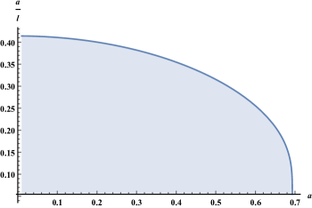
Figure 4: The MI is non-zero only in the blue shaded region.

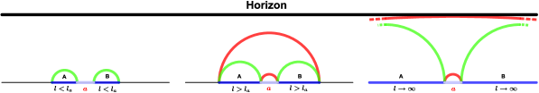
Figure 5: The geodesics relevant to MI vary as $l$ increases. As $l$ tends to infinity, the external red geodesic and two green geodesics approach the horizon in turn.

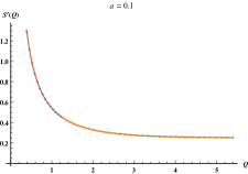
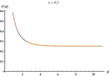
Figure 6: Generate $S^{\prime}(Q)$ iteratively. Here we set $a=0.1$ (left) and $a=0.2$ (right). The solid red line is plotted using the target analytical function. The dotted lines denote the generated function. By three iterations (blue, yellow, green), the domain of $S^{\prime}(Q)$ expands accordingly.

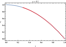
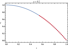
Figure 7: The reconstructed metric over $Z_{\ast a}$ (red dotted line) using MI and EE. The target metric (blue solid line) is $f=1-z^{2}$. At left and right panels, we set $a=0.1$ and $0.2$ respectively.

2.3 Entanglement of Purification

EoP is defined by the minimum EE for all possible purification of the mixed state Terhal2002 . It is closely related to MI but is an independent correlation measure Bagchi2015 . The regularization of EoP has an operational meaning in terms of Einstein-Podolsky-Rosen pairs Terhal2002 , and it is finite in the CFT Caputa1812 . In gravity side it was proposed to be related to the entanglement wedge cross section Tamaoka:2018ned ; Takayanagi:2017knl

$$E_{W}=\min_{\Sigma_{AB}}\left(\frac{Area(\Sigma_{AB})}{4}\right).$$ (28)

Here $A$ and $B$ represent two disjoint subregions on the boundary. The entanglement wedge is a bulk region surrounded by $AB\equiv A\cup B$ and the minimal surface $\Gamma_{AB}$ anchored on $AB$. $\Sigma_{AB}$ is regarded as a cross section of the entanglement wedge, which divides $\Gamma_{AB}$ into two parts. $E_{W}$ can be obtained by minimizing the area of $\Sigma_{AB}$ over all possible choices of the division.

In figure 8, we plot the geometry for non-zero EoP. We still focus on the symmetric configuration for simplicity. One can find that the EoP is zero when the MI is zero. This is because the entanglement wedge is disconnected and lacks a cross section.

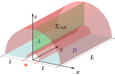
Figure 8: The entanglement wedge with non-zero EoP is a connected region wrapped by the red and blue surfaces. The green surface is the minimum cross section. EoP is determined by its area.

2.3.1 Holographic calculation

Consider the situation with $E_{W}\neq 0$. The area of $\Sigma_{AB}$ is

$$A_{\Sigma}=L^{d-2}\int_{z_{\ast}(a)}^{Z_{\ast}(Q)}\frac{dz}{\sqrt{f(z)}z^{d-1}},\,Q>Q_{a},$$ (29)

where $z_{\ast}(a)$ and $Z_{\ast}(Q)$ are the turning points of the minimal surfaces with strips of width $a$ and $Q$, respectively. Using (28), we have

$$E_{W}(Z_{\ast})=\frac{L^{d-2}}{4}\int_{z_{\ast}}^{Z_{\ast}}\frac{dz}{\sqrt{f(z)}z^{d-1}},\,Z_{\ast}>Z_{\ast a}.$$ (30)

Obviously, it is finite as $z_{\ast}>0$. Take the derivative of eq. (30), yielding

$$E_{W}^{\prime}(Z_{\ast})=\frac{L^{d-2}}{4}\frac{1}{\sqrt{f(Z_{\ast})}Z_{\ast}^{d-1}},\,Z_{\ast}>Z_{\ast a}.$$ (31)

Because this formula is structurally different from eq. (11), we cannot use the simple chain rule as before to find the metric-independent mapping $Q\mapsto Z_{\ast}$ from the change rate of the EoP with respect to $Q$.

2.3.2 Reconstruction method

We will propose a numerical method, which include four steps.

1) Discretization

Let’s discrete the metric function as $f[z[i]]$, where $i$ denotes an integer in $[0,n]$, $z[i]=i/n$, and $n$ is a large integer. Suppose that the metric $f(z)$ with $z\leq Z_{\ast}$ is given, where $Z_{\ast}$ belongs to $z[j]\leq Z_{\ast}<z[j+1]$ with the integer $j<n$. Build the dataset $\{z[i],f[z[i]]\}$ for any $i\in[0,j]$ and name it as $data_{0}$.

2) Interpolation

Append a data point $\{z[j+1],f_{1}\}$ into $data_{0}$. The value of $f_{1}$ will be specified later and the new dataset is named as $data_{1}$. Interpolate $data_{1}$ and generate the test metric function $\bar{f}(z)$ which is continuous.

3) Integration

Calculate the numerical integration

$$Q(Z_{\ast}) = 2\int_{0}^{Z_{\ast}}\frac{z^{d-1}}{\sqrt{\bar{f}(z)}\sqrt{Z_{\ast}^{2d-2}-z^{2d-2}}}dz,$$ (32)

$$\bar{E}_{W}(Z_{\ast}) = \frac{L^{d-2}}{4}\int_{z_{\ast}}^{Z_{\ast}}\frac{dz}{\sqrt{\bar{f}(z)}z^{d-1}},\,Z_{\ast}>Z_{\ast a}.$$ (33)

4) Minimization

Define a loss function

$$\mathrm{loss}(f_{1})=\left|\bar{E}_{W}(Z_{\ast})-E_{W}(Q(Z_{\ast}))\right|^{2},$$ (34)

where $E_{W}(Q)$ is the given data. Substitute eq. (32) and eq. (33) into eq. (34). Minimize the loss function and get the optimal $f_{1}$. After that, set $f[z[j+1]]=f_{1}$, $j=j+1$, and $data_{0}=data_{1}$.

Finally, iterate the steps 2), 3) and 4). Then the metric with $z>Z_{\ast}$ can be reconstructed. Note that this method is characterized by the use of a continuous interpolation function to generate the test metric and thereby we would like to refer it as the interpolation-generated method.

2.3.3 Example

For $d=2$ and $f(z)=1-z^{2}$, the EoP is Yang1810

$$E_{W}(Q)=\frac{1}{4}\log\left[\coth\left(\frac{a}{4}\right)\tanh\left(\frac{Q}{4}\right)\right],\ Q>Q_{a},$$ (35)

which provides us the main data. In addition, we need the metric below $Z_{\ast a}$, which can be given by hand or generated by the EE with $Q\leq Q_{a}$. The rest of the metric can be reconstructed using EoP. In figure 9, we plot the change of the entanglement wedge and minimum cross section as $l$ increases. In figure 10, we show the result of reconstruction, where we have specified $a=0.1$ and $n=100$. It is consistent with the left panel of figure 7 as expected.

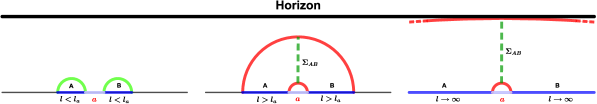
Figure 9: The entanglement wedge and its minimum cross section vary as $l$ increases. As $l$ tends to infinity, the top of the minimum cross section approaches the horizon.

​​​​​

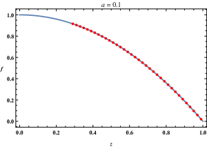
Figure 10: The reconstructed metric over $Z_{\ast a}$ (red dotted line) using the EoP, provided that the metric below $Z_{\ast a}$ is given. The target metric (blue solid line) is $f=1-z^{2}$. Here we set $a=0.1$ and $n=100$.

3 Interior of black holes

Quantum computational complexity is relevant to the number of unitary operators which converts one quantum state to another Watrous0804 . In Hashimoto:2021umd , it is found that the interior of a black hole can be reconstructed from the complexity, which is defined by ‘complexity = volume’ (CV) proposal Susskind:2014rva ; Susskind:2014moa . There are other proposals on the holographic complexity, such as ‘complexity = action’ (CA) Brown:2015bva and ‘complexity = volume 2.0’ (CV2.0) Couch:2016exn . Recently, a new infinite class of gravitational observables has been proposed to be dual to the complexity Belin:2021bga , which can be referred as ‘complexity = generalized volume’ (CGV). In this section, we will study how to reconstruct the metric in terms of CV2.0 and CGV.

3.1 Complexity = Volume 2.0

The ‘complexity 2.0’ in the gravity side can be expressed as Couch:2016exn

$$\mathcal{C}_{2.0}(t)=\frac{P}{\hbar}V(t).$$ (36)

Here, $P$ is the pressure which is related to the cosmological constant $P=-\Lambda/8\pi$ and $V(t)$ is the spacetime volume of the Wheeler-DeWitt (WDW) patch defined in a two-sided eternal AdS black holes. Note that the WDW patch is the domain of dependence of any Cauchy surface in the bulk which is anchored at the time slices on the boundary Brown:2015bva ; Carmi:2016wjl .

3.1.1 Holographic calculation

We first review the calculation of the spacetime volume $V(t)$ under the metric ansatz

$$ds^{2}=-f(r)dt^{2}+\frac{1}{f(r)}dr^{2}+r^{2}d\vec{x}^{2}.\,$$ (37)

We consider that the WDW patch moves forward in time in a symmetric way and assume that its two upper null sheets always end at the singularity, see the left panel of figure 11.

​​​​​​​​​​​​​​​​​​​​​​            

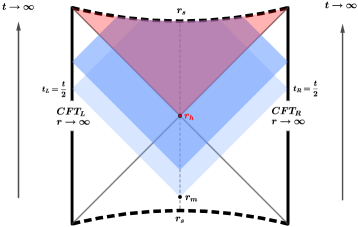
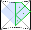
Figure 11: Left: The time evolution of the WDW patch in a two-sided AdS black hole. It is anchored at two boundary time slices $t_{L}=t/2$ and $t_{R}=t/2$. Two lower null sheets intersect at point $r_{m}$ and two upper null sheets end at the singularity $r_{s}$. As time grows, the WDW patch moves upward, through three shaded areas. The intersection $r_{m}$ will eventually approach the horizon $r_{h}$. Right: Three typical blocks of the WDW patch are labeled for the calculation of its volume.

Using the tortoise coordinate

$$r^{\ast}(r)=\int\frac{dr}{f(r)},$$

one can determine the critical time until which the complexity does not increase Carmi:2017jqz

$$t_{c}=2(r^{\ast}\left(\infty\right)-r^{\ast}(r_{s})),$$ (38)

where $r_{s}$ denotes the position of singularity. To calculate the spacetime volume, we divide the WDW patch into several parts. Due to the symmetric configuration, we just need to calculate the volumes of three regions which are labeled in the right panel of figure 11. Using the integration formula of the spacetime volume

$$V=\int_{WDW}d^{d+1}x\sqrt{-g}=\Sigma_{d-1}\int dtdrr^{d-1}$$ (39)

where $\Sigma_{d-1}$ denotes the regulated volume of the $d-1$ spatial boundary directions, we have

$$V_{1}=\Sigma_{d-1}\int_{r_{s}}^{r_{h}}drr^{d-1}(t_{R}+r^{\ast}(\infty)-r^{\ast}(r)),$$ (40)

$$V_{2}=2\Sigma_{d-1}\int_{r_{h}}^{r_{\mathrm{uv}}}drr^{d-1}(r^{\ast}(\infty)-r^{\ast}(r)),$$ (41)

$$V_{3}=\Sigma_{d-1}\int_{r_{m}}^{r_{h}}drr^{d-1}(-t_{R}+r^{\ast}(\infty)-r^{\ast}(r)),$$ (42)

where $r_{m}$ is determined by

$$t-t_{c}=2(r^{\ast}(r_{s})-r^{\ast}(r_{m}))$$ (43)

and $r_{\mathrm{uv}}$ is the UV cutoff. As a result, one can see An:2018dbz

$$\frac{dV}{dt}=\frac{\Sigma_{d-1}}{d}\left(r_{m}^{d}-r_{s}^{d}\right).$$ (44)

By setting $\delta t=t-t_{c}$ and $r_{s}=0$, we rewrite eq. (44) and eq. (43) as

$$\mathcal{C}_{2.0}^{\prime}(\delta t)=\frac{P}{\hbar}\frac{\Sigma_{d-1}}{d}r_{m}^{d},$$ (45)

$$\delta t=-2\int_{0}^{r_{m}}\frac{dr}{f(r)}.$$ (46)

3.1.2 Reconstruction method

Our data is $\mathcal{C}_{2.0}^{\prime}(\delta t)$ of the boundary field theory. Inputting the data into eq. (45), we can calculate the derivative $\delta t^{\prime}(r_{m})$. Taking the derivative on both sides of eq. (46), we obtain a very simple formula to reconstruct the metric inside the horizon

$${f(r_{m})}=-\frac{2}{\delta t^{\prime}(r_{m})}.$$ (47)

In ref. Hashimoto:2021umd , the reconstruction of the interior of black holes requires information from the exterior. Here, we have shown that this is not necessary as soon as we update the proposal from CV to CV2.0.

3.1.3 Example

Suppose $\,f(r)=r^{2}-1$ and $d=2$. Calculating eq. (46) and taking the inverse, we find

$$r_{m}=\tanh\left(\frac{\delta t}{2}\right).$$ (48)

Inserting it into (45), we read the complexity growth

$$\mathcal{C}_{2.0}^{\prime}(\delta t)=\frac{P}{\hbar}\frac{\Sigma_{1}}{2}\tanh^{2}\left(\frac{\delta t}{2}\right).$$ (49)

With the data (49) in hand, we solve eq. (45) to give

$$\delta t(r_{m})=2\,\text{arctanh}(r_{m}).$$ (50)

Using the reconstruction formula (47), we obtain the metric finally

$$f(r_{m})=r_{m}^{2}-1.$$ (51)

3.2 Complexity = Generalized Volume

Recently, the CV proposal has been generalized in Belin:2021bga . It is presented that the holographic dual of quantum complexity may be expressed as an integral of a scalar functional $F_{1}$, which depends on the background metric $g_{\mu\nu}$ and the embedding $X^{\mu}(\sigma^{a})$ of the codimension-one hypersurface $\Sigma_{F_{2}}$. The hypersurface $\Sigma_{F_{2}}$ is anchored on the time slice $\Sigma_{t}$ of the boundary and is determined by extremizing another functional $F_{2}$. In general, $F_{1}$ is different from $F_{2}$. For the simple case $F_{1}=F_{2}$, the generalized volume can be written as

$$\mathcal{C}_{gen}(t)=\max_{\partial\Sigma=\Sigma_{t}}\left[\frac{1}{L}\int_{\Sigma(t)}d^{d}\sigma\sqrt{h}F_{1}\left(g_{\mu\nu},X^{\mu}\right)\right],$$ (52)

where $L$ is the AdS radius and $h$ is the determinant of induced metric. Here we will explore the reconstruction using eq. (52), provided $F_{1}$ depends only on the curvature invariant

$$F_{1}=1+\mathcal{K}L^{4}C^{2},$$

where $C^{2}\equiv C_{\mu\nu\rho\sigma}C^{\mu\nu\rho\sigma}$ denotes the square of the Weyl tensor for the bulk spacetime and $\mathcal{K}$ is the coupling constant Belin:2021bga .

3.2.1 Holographic calculation

Let’s write the line element in the Eddington-Finkelstein coordinates

$$ds^{2}=-f(r)dv^{2}+2dvdr+r^{2}d\vec{x}^{2},$$ (53)

where $v=t+r^{\ast}(r)$. By describing the extremal hypersurface by the parametric equations $v(\sigma)$ and $r(\sigma)$, the generalized volume can be rewritten in a specific form Belin:2021bga

$$\mathcal{C}_{gen}=\Sigma_{d-1}\int_{\Sigma}d\sigma\,r^{d-1}\sqrt{-f(r)\dot{v}^{2}+2\dot{v}\dot{r}}a(r).$$ (54)

Here we have set $L=1$ and $a(r)$ is a factor about the curvature, given by

$$a(r)=1+\mathcal{K}\frac{d-2}{d}{\frac{{1}}{{r^{4}}}\left[2f(r)+r\left(rf^{\prime\prime}(r)-2f^{\prime}(r)\right)\right]}^{2}.$$ (55)

We can express the generalized volume $\mathcal{C}_{gen}$ and the boundary time $t$ in terms of the metric $f(r)$ and the minimal radius $r_{min}$ of the surface

$$\mathcal{C}_{gen}=-2\Sigma_{d-1}\int_{r_{min}}^{r_{\mathrm{uv}}}\frac{U(r)}{f(r)\sqrt{U(r_{min})-U(r)}}dr,$$ (56)

$$t=-2\int_{r_{min}}^{\infty}\frac{\sqrt{U(r_{min})}}{f(r)\sqrt{U(r_{min})-U(r)}}dr,$$ (57)

where $U(r)=-f(r)\,a^{2}(r)\,r^{2(d-1)}$ can be understood as an effective potential of a classical particle Belin:2021bga . In order to cancel $r_{min}$ in two equations above, we take derivatives:

$$\frac{d\mathcal{C}_{gen}}{dr_{min}}\!=\!2\Sigma_{d-1}\!\left\{\!\int_{r_{min}}^{\infty}\frac{U(r)U^{\prime}(r_{min})}{2f(r)[U(r_{min})-U(r)]^{\frac{3}{2}}}\!+\!\frac{U(r_{min})}{\sqrt{f(r_{min})}}\lim_{r\rightarrow r_{min}}\frac{1}{\sqrt{U(r_{min})-U(r)}}\!\right\},$$ (58)

$$\frac{dt}{dr_{min}}\!=\!\frac{2}{\sqrt{U(r_{min})}}\left\{\int_{r_{min}}^{\infty}\frac{U(r)U^{\prime}(r_{min})}{2f(r)[U(r_{min})-U(r)]^{\frac{3}{2}}}\!+\!\frac{U(r_{min})}{\sqrt{f(r_{min})}}\lim_{r\rightarrow r_{min}}\frac{1}{\sqrt{U(r_{min})-U(r)}}\right\}.$$ (59)

Using the chain rule, the time derivative of the generalized volume is given by

$$\frac{d\mathcal{C}_{gen}}{dt}=\Sigma_{d-1}\sqrt{U(r_{min})}.$$ (60)

As $t\rightarrow\infty$, this asymptotically approaches a constant

$$\frac{d\mathcal{C}_{gen}}{dt}=\lim_{t\rightarrow\infty}\Sigma_{d-1}\sqrt{U(r_{min})}=\Sigma_{d-1}\sqrt{U(r_{f})},$$ (61)

where $r=r_{f}$ is the radius of the locally maximal effective potential. Note that in the whole time evolution, we assume that the maximal extremal hypersurface changes continuously, without any sudden jumps Hashimoto:2021umd .

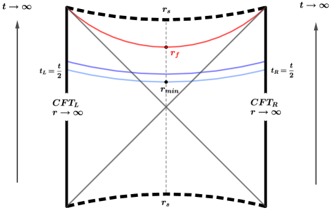
Figure 12: The time evolution of the extremal hypersurface in a two-sided AdS black hole. As time grows, the hypersurface moves up. The two nearby blue curves correspond to the hypersurfaces anchored at two adjacent times. As time tends to infinity, the hypersurface with minimal radius $r_{min}$ approaches to the one with $r_{f}$ (red curve), at which an effective potential is locally maximal.

3.2.2 Reconstruction method

Setting $\omega=r^{d}$, we rewrite (57) and (60) as

$$t=-\frac{2}{d}\int_{\omega_{min}}^{\infty}\frac{\sqrt{U(\omega_{min})}\,\omega^{\frac{1}{d}-1}}{f(\omega)\sqrt{U(\omega_{min})-U(\omega)}}d\omega,$$ (62)

$$\frac{d\mathcal{C}_{gen}}{dt}=\Sigma_{d-1}\sqrt{U(\omega_{min})},$$ (63)

where

$$U(\omega)=-f(\omega)\,a^{2}(\omega)\,\omega^{2(1-\frac{1}{d})},$$ (64)

and

$$a(\omega)=1+\mathcal{K}\frac{d-2}{d}{\frac{1}{{\omega^{\frac{4}{d}}}}}\,{\left\{2f(\omega)+\omega\,d\,\left[\omega\,d\,f^{\prime\prime}(\omega)+(d-3)f^{\prime}(\omega)\right]\right\}}.$$ (65)

To proceed, we assume that $U(\omega)$ is monotonic from $\omega_{min}$ to $\infty$. Then $U=U(\omega)$ can be inverted to a single-valued function $\omega=\omega(U)$. This allows us to change (62) as

$$\frac{t(U_{min})}{\sqrt{U_{min}}}=\int_{U_{min}}^{-\infty}{\frac{y(U)}{\sqrt{U_{min}-U}}}dU\,,$$ (66)

where we have defined a function

$$y(U)=\frac{2}{d}\frac{\,\,a^{2}(\omega)\,\,\omega^{1-\frac{1}{d}}}{U}\frac{d\omega}{dU}.$$ (67)

One can interpret (66) as the Cauchy principal value to deal with the integrand of (62) which blows up near the horizon $\omega_{h}$. Concretely, we rewrite (66) as

$$\frac{t(U_{min})}{\sqrt{U_{min}}}=\left(\int_{U_{min}}^{\epsilon}+\int_{\epsilon}^{-\epsilon}+\int_{-\epsilon}^{-\infty}\right)\frac{y(U)}{\sqrt{U_{min}-U}}dU\,,$$ (68)

where $U_{min}=U(\omega_{min})$. We assume that $\epsilon$ is small enough that the second integral $\int_{\epsilon}^{-\epsilon}$ cancels by itself. Then we have

$$\frac{t(U_{min})}{\sqrt{U_{min}}}=\left(\int_{U_{min}}^{\epsilon}+\int_{-\epsilon}^{-\infty}\right)\frac{y(U)}{\sqrt{U_{min}-U}}dU,$$ (69)

which can be further recast as

$$W(U_{min})\equiv-\frac{t(U_{min})}{\sqrt{U_{min}}}-\int_{-\infty}^{-\epsilon}\frac{y(U)}{\sqrt{U_{min}-U}}dU=\int_{\epsilon}^{U_{min}}\frac{y(U)}{\sqrt{U_{min}-U}}dU.$$ (70)

Using eq. (14), the above integral equation can be solved

$$y(U)=\frac{1}{\pi}\frac{d}{dU}\int_{\epsilon}^{U}\frac{W(U_{min})}{\sqrt{U-U_{min}}}dU_{min}.$$ (71)

Combining eq. (67), we find

$$\frac{2}{d}\frac{\,\,a^{2}(\omega)\,\,\omega^{1-\frac{1}{d}}}{U}\frac{d\omega}{dU}=\frac{1}{\pi}\frac{d}{dU}\int_{\epsilon}^{U}\frac{W(U_{min})}{\sqrt{U-U_{min}}}dU_{min}.$$ (72)

Some remarks are in order. Firstly, our main data is the derivative of the generalized volume. Using eq. (63), one can calculate the function $t(U_{min})$. In addition, we assume that the metric outside the horizon is given. As a result, we can obtain the function $W(U_{min})$. Secondly, consider the CV proposal where the factor $a=1$. One can see that eq. (72) is reduced to a first-order ordinary differential equation (ODE) of the function $\omega(U)$. Solving the ODE and using eq. (64), the metric $f(\omega)$ can be reconstructed Hashimoto:2021umd . Thirdly, for a general factor, we can insert eq. (64) and eq. (65) into eq. (72), which is changed into a complex third-order ODE of the metric function. Fortunately, it still can be solved by the canned differential equation solvers such as Mathematica’s NDSolve with the method option “EquationSimplification”$\rightarrow$“Residual” wolfram .

3.2.3 Example

Consider the AdS black hole with the target metric $f(\omega)=(\omega-1)\,\omega^{\frac{2}{d}-1}$. We read the factor (65) and the potential (64) as

$$a(\omega)=1+\kappa\left(\frac{1}{\omega}\right)^{2},$$ (73)

$$U(\omega)=-\frac{(\omega-1)(\omega^{2}+\kappa)^{2}}{\omega^{3}},$$ (74)

where $\kappa=d(d-1)^{2}(d-2)\mathcal{K}$. By analyzing the function (74), it has been pointed out that there is one local maximum inside the horizon when $-1<\kappa<\kappa_{1}=\frac{1}{8}(47-13\sqrt{13})\approx 0.016$ Belin:2021bga , see figure 13. Note that the existence of at least one local maximum inside the horizon is the requirement for the linear growth of the generalized volume.

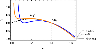
Figure 13: The effective potential $U(\omega)$ with $-1<\kappa<\kappa_{1}$ has the extremal point located at $\omega_{f}$ which is within the horizon located at $\omega_{h}=1$. $U(\omega)$ is monotonic from $\omega_{f}$ to $\infty$.

In the following, we will focus on the cases with $d=3$ and $\kappa=-0.5,0.01$. Using the target metric, we generate the data $C_{gen}^{\prime}(t)$ and the function $W(U_{min})$ we need, see figures 14 and 15. Solving the third-order ODE mentioned above with the boundary condition given by the target metric near the horizon, we reconstruct the metric inside the horizon, see figure 16. One can find that we build the metric within ($\omega_{f},\omega_{h}$) where $\omega_{f}$ depends on $\kappa$. In general, it is not possible to probe the singularity at $\omega_{s}$ if $\omega_{f}>\omega_{s}$.

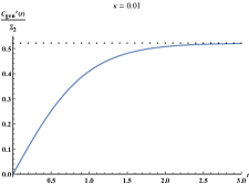
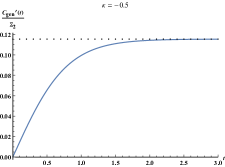
Figure 14: The change rate of generalized volume (blue solid line). At the late time, it will hit the gray dotted line, which can be described by eq. (61). The left and right correspond to $\kappa=0.01$ and $\kappa=-0.5$ respectively.

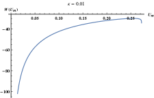
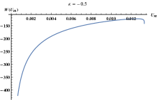
Figure 15: The function $W(U_{min})$ that is required for the reconstruction.

​​​​​​         ​​​​

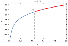
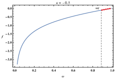
Figure 16: The reconstructed metric (red dotted line) using the generalized volume. The blue solid line is the target metric. The region deeper than $\omega_{f}$ cannot be probed.

4 Comparison

Our work is closely related to refs. Bilson:2010ff ; Hashimoto:2020mrx ; Hashimoto:2021umd , where the metric reconstruction has been studied using three measures: EE, WL and CV. Now we have extended their work to MI, EoP, CV2.0 and CGV. In table 1, we compare these seven reconstruction methods from six aspects.

1) Is the measure sensitive or insensitive to UV cutoff?

2) Is the change rate of the measure sensitive or insensitive to UV cutoff?

3) Is the measure sufficient or insufficient to reconstruct the metric?

4) Does the measure probe the exterior or interior of a black hole?

5) Does the measure depend on the spatial or temporal boundary scale?

6) Does the measure probe the spacetime in a local or non-local way?

Property	1	2	3	4	5	6
EE	Sensitive	Insensitive	Sufficient	Exterior	Spatial	Local
WL	Sensitive	Insensitive	Sufficient	Exterior	Spatial	Local
MI	Insensitive	Insensitive	Insufficient	Exterior	Spatial	Local
EoP	Insensitive	Insensitive	Insufficient	Exterior	Spatial	Local
CV	Sensitive	Insensitive	Insufficient	Interior	Temporal	Local
CV2.0	Sensitive	Insensitive	Sufficient	Interior	Temporal	Local
CGV	Sensitive	Insensitive	Insufficient	Interior	Temporal	Local

Table 1: Comparison of reconstruction methods using seven measures across six properties.

Some remarks on the comparison are in order.

i) Most of measures are sensitive to UV cutoff but their derivatives are not.

ii) For EE, WL, and CV2.0, each of them is sufficient to reconstruct the metric, given some assumptions about spacetime symmetry and structure. For other measures, the metric (or equivalent information) must be given for part of the spacetime.

iii) The measures related to the EE with spatial scales probe the exterior of black holes, while the measures related to the complexity with temporal scales probe the interior. This reflects the complementary nature of spatial entanglement and time-evolved complexity in encoding spacetime.

iv) All these measures probe the spacetime in a local way: reconstructing the metric in different radial positions requires the information at different boundary scales.

In order to better understand the last point, we will review briefly the reconstruction method by the DL from shear-viscosity data Yan:2020wcd . One can find that the holographic renormalization group flow of the shear viscosity is described by the first-order ODE Yan:2020wcd

$$\left(\eta-\frac{i\omega}{f}\right)^{\prime}+\frac{i\omega}{f}\left[z^{2}\left(\eta-\frac{i\omega}{z}\right)^{2}-\frac{1}{z^{2}}\right]=0,$$ (75)

where the metric ansatz (2) has been used. Given the metric $f(z)$ and the regular condition at horizon $\eta\left(\omega,1\right)=1+i\omega$, the ODE can be solved to yield $\eta\left(\omega,0\right)$, which is the frequency-dependent shear viscosity on the boundary field theory. In ref. Yan:2020wcd , a discretized representation of the ODE (75) is provided through a deep neural network, where the metric is encoded as trainable weights. Given the existence of the horizon and guided by the smoothness of spacetime, it is shown that three typical black hole metrics can be extracted with high accuracy from $\eta\left(\omega,0\right)$ using DL. In particular, the deep neural network exhibits an excellent generalization ability, indicating that the complete metric can be well learned from the data with narrow frequency range.

​​​

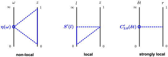
Figure 17: Three typical ways to probe the spacetime that can be described as non-local, local and strongly local, respectively. Left: The complete metric from $z=0$ to $z=1$ can be learned from the data $\eta\left(\omega\right)$ with narrow frequency range. Middle: To build the metric $f(z)$ at a given $z$, the data $S^{\prime}(l)$ with a finite range $(0,l]$ is required. Right: The metric $f(r)$ at a given $r$ can be built from the data $C^{\prime}_{2.0}(\delta t)$ around the corresponding $\delta t$.

We can classify all the reconstruction methods mentioned above into three types, the basis of which can be seen in figure 17 and explained below. The first is shear viscosity, which is characterised by the excellent generalization ability and can be understood intuitively as follows. Looking at eq. (75), one can find that in order to determine $\eta\left(\omega,0\right)$ at any non-zero frequency, the complete metric from $z=0$ to $z=1$ must be known. Conversely, each $\eta\left(\omega,0\right)$ at a non-zero frequency contains some information about the metric at any $z$. Therefore, if the technique of information mining is powerful enough, it is in principle possible to reconstruct the complete metric from a narrow frequency range, at least when the metric function is simple enough. The second involves EE, WL, MI, EoP, CV and CGV. Taking EE as an example, two equations (13) and (16) show that if we want to probe deeper into spacetime, we need data $S^{\prime}(l)$ at larger $l$. In addition, to build $f(z)$ at a given $z$, the data $S^{\prime}(l)$ with a finite range $(0,l]$ is required. The third is CV2.0. From (45)-(47) and the left panel of figure 11, we know that it probes the shallower spacetime as the data $\mathcal{C}_{2.0}^{\prime}(\delta t)$ with larger $\delta t$ is input. Moreover, one can reconstruct the metric $f(r)$ at certain $r$ if and only if a small range of data $\mathcal{C}_{2.0}^{\prime}(\delta t)$ around the corresponding $\delta t$ is provided, see figure 18. We therefore argue that the reconstruction method using CV2.0 has a certain strong locality. Despite its distinctiveness, CV2.0 still shares some commonality with the second type: reconstructing metrics of different radial positions always requires the data of different boundary scales. Note that here the measures can be relevant to entanglement or complexity, and the boundary scale can be either spatial or temporal.

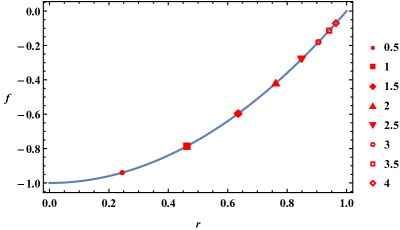
Figure 18: The bulk metric reconstruction with strong locality. The red labels denote the reconstruction results using the data $\mathcal{C}_{2.0}^{\prime}(\delta t)$ around given $\delta t$. The blue solid line is the target metric. We choose eight $\delta t$ which are listed on the right. The small ranges around them are fixed as $[\delta t-0.1\delta t,\delta t+0.1\delta t]$. Within each small range, we take a uniform sample of 100 points as our data.

5 Summary

Following the spirit of ‘It from Qubit’ simons , we investigate the bulk reconstruction of black hole metrics using various quantum information measures on the boundary field theories. We propose several reconstruction methods all of which are free of UV divergence. One can see that different mathematical ingredient appears in each method: analytic formulas for EE, iterative data generation for MI, interpolation-generated test metrics for EoP, simple derivatives for CV2.0, and a complex three-order ODE for CGV. We also witness the complementarity of entanglement and complexity, and analyse the differences and similarities among different probing ways. Our results would enrich the understanding of how field theory encodes gravity.

In the future, it would be important to reduce the assumptions of the reconstruction methods and thus broaden their applicability. In this regard, one can draw lessons from the bulk reconstruction that do not rely on spacetime symmetries Bao:2019bib ; Cao:2020uvb , as well as the illumination on entanglement shadows Hubeny1306 ; Bala1406 ; Freivogel1412 . Meanwhile, one can collect experimental and simulated data on quantum information measures in strongly coupled field theories with gravity duals. It would be intriguing to explore whether the reconstruction methods can extract reasonable holographic spacetimes from these data.

References

- (1) J.M. Maldacena, The Large N limit of superconformal field theories and supergravity, Adv. Theor. Math. Phys. 2 (1998) 231[hep-th/9711200].
- (2) S.S. Gubser, I.R. Klebanov and A.M. Polyakov, Gauge theory correlators from noncritical string theory, Phys. Lett. B 428 (1998) 105 [hep-th/9802109].
- (3) E. Witten, Anti-de Sitter space and holography, Adv. Theor. Math. Phys. 2 (1998) 253 [hep-th/9802150].
- (4) L. Susskind and E. Witten, The Holographic bound in anti-de Sitter space, (1998) [hep-th/9805114].
- (5) H. Liu and J. Sonner, Quantum many-body physics from a gravitational lens, Nature Rev. Phys. 2 (2020) 615 [arXiv:2004.06159].
- (6) A. Hamilton, D.N. Kabat, G. Lifschytz and D.A. Lowe, Holographic representation of local bulk operators, Phys. Rev. D 74 (2006) 066009 [hep-th/0606141].
- (7) T. De Jonckheere, Modave lectures on bulk reconstruction in AdS/CFT, PoS Modave2017 (2018) 005 [arXiv:1711.07787].
- (8) D. Harlow, TASI Lectures on the emergence of bulk physics in AdS/CFT, PoS TASI2017 (2018) 002 [arXiv:1802.01040].
- (9) N. Kajuri, Lectures on bulk reconstruction, SciPost Phys. Lect. Notes 22 (2021) [arXiv:2003.00587].
- (10) S. de Haro, S.N. Solodukhin and K. Skenderis, Holographic reconstruction of space-time and renormalization in the AdS / CFT correspondence, Commun. Math. Phys. 217 (2001) 595 [hep-th/0002230].
- (11) J. Hammersley, Extracting the bulk metric from boundary information in asymptotically AdS spacetimes JHEP 12 (2006) 047 [hep-th/0609202].
- (12) V.E. Hubeny, H. Liu and M. Rangamani, Bulk-cone singularities & signatures of horizon formation in AdS/CFT JHEP 01 (2007) 009 [hep-th/0610041].
- (13) J. Hammersley, Numerical metric extraction in AdS/CFT, Gen. Rel. Grav. 40 (2008) 1619 [arXiv:0705.0159].
- (14) S. Bilson, Extracting spacetimes using the AdS/CFT conjecture, JHEP 08 (2008) 073 [ arXiv:0807.3695].
- (15) S. Bilson, Extracting Spacetimes using the AdS/CFT Conjecture: Part II, JHEP 02 (2011) 050 [ arXiv:1012.1812].
- (16) V.E. Hubeny, Extremal surfaces as bulk probes in AdS/CFT, JHEP 07 (2012) 093 [arXiv:1203.1044].
- (17) V. Balasubramanian, B.D. Chowdhury, B. Czech, J. de Boer and M.P. Heller, Bulk curves from boundary data in holography, Phys. Rev. D 89 (2014) 086004 [arXiv:1310.4204].
- (18) R.C. Myers, J. Rao and S. Sugishita, Holographic Holes in Higher Dimensions, JHEP 06 (2014) 044 [arXiv:1403.3416].
- (19) B. Czech and L. Lamprou, Holographic definition of points and distances, Phys. Rev. D 90 (2014) 106005 [arXiv:1409.4473].
- (20) N. Engelhardt and G.T. Horowitz, Towards a Reconstruction of General Bulk Metrics, Class. Quant. Grav. 34 (2017) 015004 [arXiv:1605.01070].
- (21) N. Engelhardt and G.T. Horowitz, Recovering the spacetime metric from a holographic dual, Adv. Theor. Math. Phys. 21 (2017) 1635 [arXiv:1612.00391].
- (22) S.R. Roy and D. Sarkar, Bulk metric reconstruction from boundary entanglement, Phys. Rev. D 98 (2018) 066017 [arXiv:1801.07280].
- (23) D. Kabat and G. Lifschytz, Emergence of spacetime from the algebra of total modular Hamiltonians, JHEP 05 (2019) 017 [arXiv:1812.02915].
- (24) K. Hashimoto, Building bulk from Wilson loops, PTEP 2021 (2021) 023B04 [arXiv:2008.10883].
- (25) S. Caron-Huot, Holographic cameras: An eye for the bulk, JHEP 03 (2023) 047 [arXiv:2211.11791].
- (26) J.M. Maldacena, Eternal black holes in anti-de Sitter, JHEP 04 (2003) 021 [hep-th/0106112].
- (27) S. Ryu and T. Takayanagi, Holographic derivation of entanglement entropy from AdS/CFT, Phys. Rev. Lett. 96 (2006) 181602 [hep-th/0603001].
- (28) M. Van Raamsdonk, Building up spacetime with quantum entanglement, Gen. Rel. Grav. 42 (2010) 2323 [arXiv:1005.3035].
- (29) B. Swingle, Entanglement Renormalization and Holography, Phys. Rev. D 86 (2012) 065007 [arXiv:0905.1317].
- (30) J. Maldacena and L. Susskind, Cool horizons for entangled black holes, Fortsch. Phys. 61 (2013) 781 [arXiv:1306.0533].
- (31) M. Rangamani, T. Takayanagi, Aspects of Holographic Entanglement Entropy, JHEP 08 (2018) 045 [hep-th/0605073].
- (32) L. Susskind, Entanglement is not enough, Fortsch. Phys. 64 (2016) 49 [arXiv:1411.0690].
- (33) L. Susskind, Computational Complexity and Black Hole Horizons, Fortsch. Phys. 64 (2016) 24 [arXiv:1403.5695].
- (34) K. Hashimoto and R. Watanabe, Bulk reconstruction of metrics inside black holes by complexity, JHEP 09 (2021) 165 [arXiv:2103.13186].
- (35) K. Skenderis, Lecture notes on holographic renormalization, Class. Quantum. Gravity 19 (2002) 5849 [hep-th/0209067].
- (36) I. Papadimitriou, Lectures on Holographic Renormalization, Springer Proceedings in Physics Vol. 176: Theoretical Frontiers in Black Holes and Cosmology, Springer Press (2016).
- (37) N. Jokela and A. Pönni, Towards precision holography, Phys. Rev. D 103 (2021) 026010 [arXiv:2007.00010].
- (38) K. Hashimoto, S. Sugishita, A. Tanaka and A. Tomiya, Deep learning and the AdS/CFT correspondence, Phys. Rev. D 98 (2018) 046019 [arXiv:1802.08313].
- (39) K. Hashimoto, S. Sugishita, A. Tanaka and A. Tomiya, Deep Learning and Holographic QCD, Phys. Rev. D 98 (2018) 106014 [arXiv:1809.10536].
- (40) K. Hashimoto, AdS/CFT correspondence as a deep Boltzmann machine, Phys. Rev. D 99 (2019) 106017 [arXiv:1903.04951].
- (41) J. Tan and C.B. Chen, Deep learning the holographic black hole with charge, Int. J. Mod. Phys. D 28 (2019) 1950153 [arXiv:1908.01470].
- (42) T. Akutagawa, K. Hashimoto and T. Sumimoto, Deep Learning and AdS/QCD, Phys. Rev. D 102 (2020) 026020 [arXiv:2005.02636].
- (43) Y.K. Yan, S.F. Wu, X.H. Ge and Y. Tian, Deep learning black hole metrics from shear viscosity, Phys. Rev. D 102 (2020) 101902(R) [arXiv:2004.12112].
- (44) K. Hashimoto, H.Y. Hu and Y.Z. You, Neural ordinary differential equation and holographic quantum chromodynamics, Mach. Learn. Sci. Tech. 2 (2021) 035011 [arXiv:2006.00712].
- (45) K. Hashimoto, K. Ohashi and T. Sumimoto, Deriving the dilaton potential in improved holographic QCD from the meson spectrum, Phys. Rev. D 105 (2022) 106008 [arXiv:2108.08091].
- (46) R. Katsube, W.H. Tam, M. Hotta and Y. Nambu, Deep learning metric detectors in general relativity, Phys. Rev. D 106 (2022) 044051 [arXiv:2206.03006].
- (47) K. Hashimoto, K. Ohashi and T. Sumimoto, Deriving dilaton potential in improved holographic QCD from chiral condensate, PTEP 2023 (2023) 033B01 [arXiv:2209.04638].
- (48) K. Li, Y. Ling, P. Liu and M.H. Wu, Learning the black hole metric from holographic conductivity, Phys. Rev. D 107 (2023) 066021 [arXiv:2209.05203].
- (49) Y.Z. You, Z. Yang and X.L. Qi, Machine Learning Spatial Geometry from Entanglement Features, Phys. Rev. B 97 (2018) 045153 [arXiv:1709.01223].
- (50) H.Y. Hu, S.H. Li, L. Wang and Y.Z. You, Machine Learning Holographic Mapping by Neural Network Renormalization Group, Phys. Rev. Res. 2 (2020) 023369 [arXiv:1903.00804].
- (51) X. Han and S.A. Hartnoll, Deep Quantum Geometry of Matrices, Phys. Rev. X 10 (2020) 011069 [arXiv:1906.08781].
- (52) J. Lam and Y.Z. You, Machine learning statistical gravity from multi-region entanglement entropy, Phys. Rev. Res. 3 (2021) 043199 [arXiv:2110.01115].
- (53) M.M. Wolf, F. Verstraete, M.B. Hastings and J.I. Cirac, Area Laws in Quantum Systems: Mutual Information and Correlations, Phys. Rev. Lett. 100 (2008) 070502 [arXiv:0704.3906].
- (54) B.M. Terhal, M. Horodecki, D.W. Leung and D.P. DiVincenzo, The entanglement of purification, J. Math. Phys. 43 (2002) 4286 [quant-ph/0202044].
- (55) J. Couch, W. Fischler and P.H. Nguyen, Noether charge, black hole volume, and complexity, JHEP 03 (2017) 119 [arXiv:1610.02038].
- (56) A. Belin, R.C. Myers, S.M. Ruan, G.Sárosi and A.J. Speranza, Does complexity equal anything?, Phys. Rev. Lett. 128 (2022) 081602 [arXiv:2111.02429].
- (57) A.D. Polyanin, Handbook of Integral Equations, CRC Press. (1998)
- (58) W. Fischler, A. Kundu and S. Kundu, Holographic mutual information at finite temperature, Phys. Rev. D 87 (2013) 126012 [arXiv:1212.4764].
- (59) B. Swingle, Mutual information and the structure of entanglement in quantum field theory, October 2010 [ arXiv:1010.4038].
- (60) R. Espíndola, A. Guijosa and J.F. Pedraza, Entanglement wedge reconstruction and entanglement of purification, Eur. Phys. J. C 78 (2018) 646 [arXiv:1804.05855].
- (61) S. Bagchi and A.K. Pati, Monogamy, polygamy, and other properties of entanglement of purification, Phys. Rev. A 91 (2015) 042323 [arXiv:1502.01272].
- (62) P. Caputa, M. Miyaji, T. Takayanagi, K. Umemoto, Holographic entanglement of purification from conformal field theories, Phys. Rev. Lett. 122 (2019) 111601 [arXiv:1812.05268].
- (63) T. Takayanagi and K. Umemoto, Entanglement of purification through holographic duality, Nature Phys. 14 (2018) 573 [arXiv:1708.09393].
- (64) K. Tamaoka, Entanglement Wedge Cross Section from the Dual Density Matrix, Phys. Rev. Lett. 122 (2019) 141601 [arXiv:1809.09109].
- (65) R.Q. Yang, C.Y. Zhang and W.M. Li, Holographic entanglement of purification for thermofield double states and thermal quench, JHEP 01 (2019) 114 [arXiv:1810.00420].
- (66) J. Watrous, Quantum Computational Complexity, [ arXiv:0804.3401].
- (67) A.R. Brown, D.A. Roberts, L. Susskind, B. Swingle and Y. Zhao, Holographic Complexity Equals Bulk Action?, Phys. Rev. Lett. 116 (2016) 191301 [arXiv:1509.07876].
- (68) D. Carmi, R.C. Myers and P. Rath, Comments on Holographic Complexity, JHEP 03 (2017) 118 [arXiv:1612.00433].
- (69) D. Carmi, S. Chapman, H. Marrochio, R.C. Myers and S. Sugishita, On the Time Dependence of Holographic Complexity, JHEP 11 (2017) 188 [ arXiv:1709.10184].
- (70) Y.S. An, R.G. Cai and Y. Peng, Time Dependence of Holographic Complexity in Gauss-Bonnet Gravity, Phys. Rev. D 98 (2018) 106013 [arXiv:1805.07775].
- (71) Wolfram Language and System Documentation Center. Numerical Solution of Differential-Algebraic Equations.
- (72) F. Omidi, Generalized Volume-Complexity For Two-Sided Hyperscaling Violating Black Branes, JHEP 01 (2023) 105 [arXiv:2207.05287].
- (73) A.R. Brown, D.A. Roberts, L. Susskind, B. Swingle and Y. Zhao, Complexity, action, and black holes, Phys. Rev. D 93 (2016) 086006 [arXiv:1512.04993].
- (74) P. Burda, R. Gregory and A. Jain, Holographic reconstruction of bubble spacetimes, Phys. Rev. D 99 (2019) 026003 [arXiv:1804.05202].
- (75) S. Hernández-Cuenca and G.T. Horowitz, Bulk reconstruction of metrics with a compact space asymptotically, JHEP 08 (2020) 108 [arXiv:2003.08409].
- (76) Simons foundation: It from Qubit: Simons collaboration on quantum Fields, gravity and information.
- (77) N. Bao, C. Cao, S. Fischetti and C. Keeler, Towards Bulk Metric Reconstruction from Extremal Area Variations, Class. Quant. Grav. 36 (2019) 185002 [arXiv:1904.04834].
- (78) C. Cao, X.L. Qi, B. Swingle and E. Tang, Building Bulk Geometry from the Tensor Radon Transform, JHEP 12 (2020) 033 [arXiv:2007.00004].
- (79) V.E. Hubeny, H. Maxfield, M. Rangamani and E. Tonni, Holographic entanglement plateaux, JHEP 08 (2013) 092 [arXiv:1306.4004].
- (80) V. Balasubramanian, B.D. Chowdhury, B. Czech and J. de Boer, Entwinement and the emergence of spacetime, JHEP 01 (2015) 048 [arXiv:1406.5859].
- (81) B. Freivogel, R. Jefferson, L. Kabir, B. Mosk and I.-S. Yang, Casting shadows on holographic reconstruction, Phys. Rev. D 91 (2015) 086013 [arXiv:1412.5175].
- (82) N. Jokela, A. Pönni, T. Rindlisbacher, K. Rummukainen and A. Salami, Disentangling the gravity dual of Yang-Mills theory, [arXiv:2304.08949].