Accuracy in readout of glutamate concentrations by neuronal cells.

Abstract

Glutamate and glycine are important neurotransmitters in the brain. An action potential propagating in the terminal of a presynatic neuron causes the release of glutamate and glycine in the synapse by vesicles fusing with the cell membrane, which then activate various receptors on the cell membrane of the post synaptic neuron. Entry of $Ca^{2+}$ through the activated NMDA receptors leads to a host of cellular processes of which long term potentiation is of crucial importance because it is widely considered to be one of the major mechanisms behind learning and memory. By analysing the readout of glutamate concentration by the post synaptic neurons during $Ca^{2+}$ signaling, we find that the average receptor density in hippocampal neurons has evolved to allow for accurate measurement of the glutamate concentration in the synaptic cleft.

I Introduction

Cells have evolved to be exceptional information processing machines. E Coli can detect concentrations of 3.2 nM of the attractant aspartate which is equivalent to around three molecules in the cell volume [1],[2]. Receptors in the retina can detect a single photon [3]. Eukaryotic cells are known to measure and respond to extremely shallow gradients of chemical signals [4],[5],[6]. Understanding of limitations to cellular measurement theoretically was first carried out in the work of Berg and Purcell [8] who showed that the chemotatic sensitivity of EColi approaches that allowed by optimal design. Since then theoretical works have studied various aspects of the problem, from the role of receptor kinetics and receptor cooperativity [9],[10] in concentration measurements, to reduction in noise in concentration measurements because of cellular communication [12], to limitation in measurement of temporal concentration changes [11]. Even limitations to the measurement of cellular gradients were considered in a host of works [13]-[20].

The list of theoretical works mentioned above is far from exhaustive, however majority of such studies in literature have tried to understand the problem of limitations to cellular measurements by reducing the cell to a spherical object with measurements done by cell surface receptors without any reference to the activities in the cellular cytoplasm. However the processing of extracellular signals is done through the reactions happening in the cellular cytoplasm. Understanding limitations to cellular measurements carried out using reactions happening in the cellular cytoplasm as readouts is relatively unexplored in literature. In neuronal cells the problem of limitations on measurements of neurotransmitter concentrations has not been studied theoretically despite its importance given that neurons communicate using the neurotransmitters that are released in the synapse. In the post synaptic neurons the membrane potential reaching a threshold value causes $Na^{+}$ channels on the membrane to open up resulting in a substantial influx of $Na^{+}$ ions into the cells leading to the depolarizing phase of an action potential that leads to the membrane potential shooting up. In the depolarizing phase $Ca^{2+}$ also enters the post synaptic neuron through activation of the NMDA receptors. This $Ca^{2+}$ attaches to calmodulin in the cytoplasm which then attaches to kinases including CaMKII causing their activation. Activated CaMKII phosphorylates AMPA receptors thereby increasing the conduction of sodium ions. It also increases the movement of AMPA receptors to the neuronal membrane thereby increasing the amount of $Na^{+}$ that could move inside the neuronal cell. This leads to synaptic enhancement and leads to long term potentiation, a important cellular mechanism that underlies learning and memory. In order for this process to be robust, it is penultimate that synaptic enhancement be linked to the strength of the action potential in the pre-synaptic neuron. As the action potential subsides the $Na^{+}$ and $K^{+}$ channels are closed and the corresponding ion concentrations in the neuron are set back to the resting stage. The NMDA receptor gets activated when two glutamate and two glycine ligands are attached to it. Excessive glutamate release and over expression of NMDAR’s has been linked to NMDAR-dependent neurotoxicity in several CNS disorders, including ischaemic stroke and neurodegenerative disorders such as Parkinson disease, Alzheimer disease and Huntington disease, while less than optimal glutamate release has been linked to depression and other psychiatric disorders[21]. It is hence natural that the neurons should be employed with mechanisms that detect the glutamate concentrations with appropriate accuracy. In this work, we evaluate the limitations to measurement of glutmate concentration in neuronal cells and show that the average receptor density in hippocampal neurons is poised to allow for optimal measurement of these concentrations.

Theory

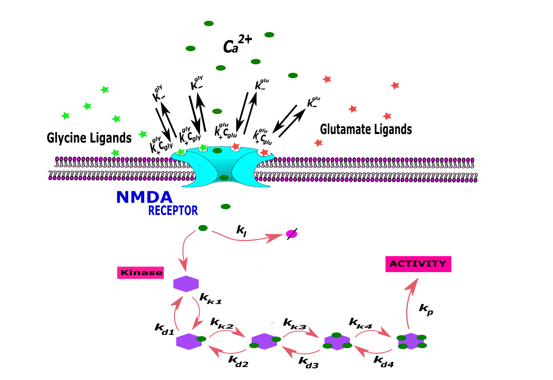
Figure 1: Schematic representation of elements of the $Ca^{2+}$ signal transduction pathway that are studied in the paper. The rate equations for the reactions are presented in Eq.1.

In order to consider the readout of the glutamate concentration by the neuron consider the schemata of reactions in Fig.1. The concentration of the glutamate/glycine ligands is represented by $c_{glu}/c_{gly}$. Two glutamine and glycine ligands are required to attach to the NMDA receptor in order for it to open to $Ca^{2+}$ influx. The rate of attachment of the ligand to the NMDA receptor is denoted as $k_{+}^{glu}c_{glu}/k_{+}^{gly}c_{gly}$ and the rate of detachment is $k_{-}^{glu}/k_{-}^{gly}$. The attachment of the ligands to the NMDA receptors opens up $Ca^{2+}$ channel in the receptor leading to influx of $Ca^{2+}$, whose concentration inside the cell is represented by $C_{Ca}(t)$. The $Ca^{2+}$ then attaches to Calmodulin which has four calcium binding sites organized into two globular domains. The C terminal lobe contains two high-affinity $Ca^{2+}$ -binding sites, while the N-terminal lobe contains two sites with lower $Ca^{2+}$ affinity. Since we expect the attachment of calcium to these domains to happen sequentially, we model the attachment of the first $Ca^{2+}$ to calmoudlin to produce a $K-Ca$ at the rate $k_{k1}$. The detachment rate of $Ca^{2+}$ from $K-Ca$ is taken to be $k_{d1}$. We model the attachment of the $Ca^{2+}$ to $K-Ca$ to produce a $K-Ca-Ca$ at the rate $k_{k2}$. The detachment rate of $Ca^{2+}$ from $K-Ca-Ca$ is taken to be $k_{d2}$. We similarly define $k_{k3},k_{k4}$ and $k_{d3},k_{d4}$. The $K-Ca-Ca-Ca-Ca$ complex phosphorylates AMPA receptors as well as increases the movement of AMPA receptors to the plasma membrane. We model this activity happening at a rate $k_{p}$, the amount of which we label by $C_{Pr}$. Let $k_{dp}$ be the rate at which this activity gets reduced. Finally the $Ca^{2+}$ coming into the cell has to also be removed from the cell. This happens at a rate $k_{l}$. We denote by $N$ the rate at which $Ca^{2+}$, enters the cell when the $Ca^{2+}$ channel is open. Assume that the ligands attach the receptor at times $t^{j}_{2i-1}$ and detach at times $t^{j}_{2i}$, with $T$ representing the time duration of the action potential which is the measurement time and $j=1,2,3,4$ correspond to the first glutamine ligand, the second glutamine ligand, the first glycine ligand and the second glycine ligand respectively. Also let us assume the probability of realizing these attachment detachment events is presented by $P(\{t_{i}^{j}\})$. We have the following rate equations

$$\begin{split}\frac{dC_{Ca}}{dt}&=N\Pi_{j=1,4}[\sum_{t^{j}_{i}<T}(-1)^{i-1}\Theta(t-t^{j}_{i})]-(k_{l}+k_{k1}C_{K}+k_{k2}C_{K-Ca}+k_{k3}C_{K-Ca-Ca}+k_{k4}C_{K-Ca-Ca-Ca})C_{Ca}+\\ &k_{d1}C_{K-Ca}+k_{d2}C_{K-Ca-Ca}+k_{d3}C_{K-Ca-Ca-Ca}+k_{d4}C_{K-Ca-Ca-Ca-Ca}\\ \frac{dC_{K}}{dt}&=k_{d1}C_{K-Ca}-k_{k1}C_{Ca}C_{K}\\ \frac{dC_{K-Ca}}{dt}&=k_{k1}C_{Ca}C_{K}+k_{d2}C_{K-Ca-Ca}-k_{d1}C_{K-Ca}\\ \frac{dC_{K-Ca-Ca}}{dt}&=k_{k2}C_{K-Ca}C_{Ca}+k_{d3}C_{K-Ca-Ca-Ca}-k_{d2}C_{K-Ca-Ca}\\ \frac{dC_{K-Ca-Ca-Ca}}{dt}&=k_{k3}C_{K-Ca-Ca}C_{Ca}+k_{d4}C_{K-Ca-Ca-Ca-Ca}-k_{d3}C_{K-Ca-Ca-Ca}\\ \frac{dC_{K-Ca-Ca-Ca-Ca}}{dt}&=k_{k4}C_{K-Ca-Ca-Ca}C_{Ca}-k_{d4}C_{K-Ca-Ca-Ca-Ca}\\ \frac{dC_{Pr}}{dt}&=k_{p}C_{K-Ca-Ca-Ca-Ca}-k_{dp}C_{Pr}\\ \end{split}$$ (1)

where, $\Theta(x)$ is

$$\Theta(x)=\begin{cases}1,\;x>0,\\ 0,\;x<0.\end{cases}$$

The association and dissociation rate constant of glutamate with the NMDA receptor are [33] $k+\approx 10^{7}M^{-1}s^{-1}$, $k_{-}\sim 8s^{-1}$ respectively. The concentration of glutamate in the synaptic cleft is also understood to be of the order of a few millimolars [34]. As such one would have expected the probability of occupancy of a NMDA receptor to be $\frac{k_{+}c}{k_{+}c+k_{-}}\approx 1$. However, the glutamate concentration rapidly diffuses after arriving at the synaptic cleft through a vesicle. The decay is exponential with a time constant $\sim 3ms$. [37] found that because of this rapid diffusion, for the range of glutamate molecules in a vesicle $(1500-4000)$ [35], [36] and value of most likely diffusion constant $D=.25\mu m^{2}/s$ the receptor occupancy (with two glutamate molecules) was $30-81$ percent. Glycine concentration in the synaptic cleft would also be expected to similarly diffuse out on similar time scales and given that the rate constants are of a similar magnitude [38] would lead to similar receptor occupancy. The probability of receptor occupancy (we are considering either glutamate or glycine here) obeys the equation

$$\frac{dp_{2}}{dt} =k_{+}cp_{1}-k_{-}p_{2}$$

$$\frac{dp_{1}}{dt} =k_{+}c(1-p_{1}-p_{2})-k_{-}p_{1}=k_{+}c-(k_{+}c+k_{-})p_{1}-k_{+}cp_{2}$$

where $p_{1}/p_{2}$ is the probability of the receptor being occupied with one/two glutamate (or glycine) molecule(s). If we define $\frac{k_{+}c}{k_{-}}=k$ and $k_{-}t=t^{\prime}$. The above can be written as

$$\frac{dp_{2}}{dt^{\prime}} =kp_{1}-p_{2}$$

$$\frac{dp_{1}}{dt^{\prime}} \approx k-(k+1)p_{1}-kp_{2}$$

or

$$\frac{1}{k}(\frac{d^{2}p_{2}}{dt^{\prime 2}}+\frac{dp_{2}}{dt^{\prime}}) \approx k-\frac{k+1}{k}\frac{dp_{2}}{dt^{\prime}}-\frac{k+1}{k}p_{2}-kp_{2}$$

which gives assuming $k>>1$, gives

$$k^{2}-(k+1)\frac{dp_{2}}{dt^{\prime}}-(k^{2}+k+1)p_{2}\approx 0$$ (3)

implying

$$p_{2}(T)=\frac{k^{2}}{k^{2}+k+1}\left(1-e^{-\frac{\left(k^{2}+k+1\right)(k_{-}T)}{k+1}}\right)$$ (4)

We see that plugging $T=3ms$ gives $p(T)\sim 1$. Diffusion removing the glutamate out of the synaptic cleft, however implies that we have to consider a renormalized value of $k_{+}c$ so as to get $p(T)$ between $.30-.81$, hence the renormalized values of $k_{+}c$ should be such that $k_{+}cT\in[.4,1.7]$. Note that $\frac{k_{+}c}{k_{-}}$ is still $>>1$ in this range and since this approximation was used above, Eq.3 is still valid. Now going back to Eq.1, if we were to assume that the measurement time to be so short that,

1. It only resulted in only $2$ glutamine and $2$ glycine attachment events, such that $t_{7}$ is the time of the last attachment event, with no detachment event.

2. Except for the rate equation for $C_{K}$ the first term on the R.H.S is the most dominant in every equation,

we would have

$$\begin{split}C_{Ca}(t)&=N(t-t_{7})\\ C_{K-Ca}(t)&=Nk_{k1}C_{K}\frac{(t-t_{7})^{2}}{2}\\ C_{K-Ca-Ca}(t)&=N^{2}k_{k1}k_{k2}C_{K}\frac{(t-t_{7})^{4}}{2\times 4}\\ C_{K-Ca-Ca-Ca}(t)&=N^{3}k_{k1}k_{k2}k_{k3}C_{K}\frac{(t-t_{7})^{6}}{2\times 4\times 6}\\ C_{K-Ca-Ca-Ca-Ca}(t)&=N^{4}k_{k1}k_{k2}k_{k3}k_{k4}C_{K}\frac{(t-t_{7})^{8}}{2\times 4\times 6\times 8}\\ C_{Pr}&=N^{5}k_{k1}k_{k2}k_{k3}k_{k4}k_{p}C_{K}\frac{(t-t_{7})^{9}}{2\times 4\times 6\times 8\times 9}\end{split}$$ (5)

Now, at rest most neurons have an intracellular calcium concentration of about $50-100$ nM that can rise transiently during electrical activity to levels that are 10 to 100 times higher [41] in around a millisecond. We can hence assume that $N=10000nM/ms=10^{-2}Ms^{-1}$. From [42] we find $k_{d1},k_{d2}=500$ $s^{-1}$, $k_{d3},k_{d4}=6$ $s^{-1}$. An estimate of calmodulin concentration used in literature is $C_{K}=10^{-4}$M [43]. The association rate of $Ca^{2+}$ with calmodulin taken from literature [44] is between $k_{k3},k_{k4}=6.8\times 10^{6}\;M^{-1}s^{-1}$ and $k_{k1},k_{k2}=108\times 10^{6}\;M^{-1}s^{-1}$. Hence

$$\begin{split}C_{K}(t)&\sim 10^{-4}M\\ C_{Ca}(t)&\sim 10^{-2}\times 10^{-3}=10^{-5}M\\ C_{K-Ca}(t)&\sim 10^{-2}\times(100\times 10^{6})\times 10^{-4}\times 10^{-6}M=10^{-4}M\\ C_{K-Ca-Ca}(t)&\sim 10^{-4}\times(100\times 10^{6})^{2}\times 10^{-4}\times 10^{-12}\times 10^{-1}M=10^{-5}M\\ C_{K-Ca-Ca-Ca}(t)&\sim 10^{-6}\times(10\times 10^{6})\times(100\times 10^{6})^{2}\times 10^{-4}\times 10^{-18}\times 10^{-1}M=10^{-6}M\\ C_{K-Ca-Ca-Ca-Ca}(t)&\sim 10^{-8}\times(10\times 10^{6})^{2}\times(100\times 10^{6})^{2}\times 10^{-4}\times 10^{-24}\times 10^{-2}M=10^{-8}M\\ \end{split}$$ (6)

The $\sim$ above implies an order of magnitude estimate. Note that any of the $k_{k1},k_{k2},k_{k3},k_{k4}$ multiplied by $C_{Ca}(t)$ gives a factor of atleast $10^{2}$. Also from above we see that addition of every $Ca^{2+}$ to a molecule reduces its concentration atleast by a factor of $10$. This then justifies the claim that the first term on the R.H.S is the most dominant on the R.H.S in every equation and hence our assumption in derivation of Eq.5 is consistent. This is also seen in Fig.2 where error evaluated assuming $C_{Cpr}$ from Eq.5 is similar to error evaluated using $C_{Cpr}$ obtained from Eq.1.

We note that if we were to associate the rates $108\times 10^{6}\;M^{-1}s^{-1}$, $6.8\times 10^{6}\;M^{-1}s^{-1}$ to a different permutation of $k_{k1},k_{k2},k_{k3},k_{k4}$ (for e.g. $k_{k2},k_{k4}=6.8\times 10^{6}\;M^{-1}s^{-1}$ and $k_{k1},k_{k3}=108\times 10^{6}\;M^{-1}s^{-1}$)with the corresponding permutations of $k_{d1},k_{d2},k_{d3},k_{d4}$, we would still have the first term on the R.H.S of rate equations of Eq.1, except for the rate equation for $C_{K}$, to be dominant. This would then cause the error in measurement of glutamate concentration to be independent of the reaction rates in the cytoplasm. Hence as far as the problem of evaluation of the value of error in concentration measurement goes, the order of attachment of glutamate to the NMDA receptor is irrelevant.

To see this, let us for example consider the equation

$$\frac{dC_{K-Ca-Ca-Ca}}{dt} =k_{k3}C_{K-Ca-Ca}C_{Ca}+k_{d4}C_{K-Ca-Ca-Ca-Ca}-k_{d3}C_{K-Ca-Ca-Ca}$$

If we consider ratio of terms on the right hand side, we get

$$k_{k3}C_{K-Ca-Ca}C_{Ca}:k_{d4}C_{K-Ca-Ca-Ca-Ca}:k_{d3}C_{K-Ca-Ca-Ca} =$$

$$k_{k3}C_{Ca}:k_{d4}\frac{C_{K-Ca-Ca-Ca-Ca}}{C_{K-Ca-Ca}}:k_{d3}\frac{C_{K-Ca-Ca-Ca}}{C_{K-Ca-Ca}} =$$

$$k_{k3}C_{Ca}:\frac{k_{d4}k_{k3}k_{k4}N^{2}(t-t_{7})^{4}}{6\times 8}:\frac{k_{d3}k_{k3}N(t-t_{7})^{2}}{6} =$$

$$k_{k3}C_{Ca}:\frac{k_{d4}k_{k3}C_{Ca}k_{k4}N(t-t_{7})^{3}}{6\times 8}:\frac{k_{d3}k_{k3}C_{Ca}(t-t_{7})}{6} =$$

$$1:\frac{k_{d4}k_{k4}N(t-t_{7})^{3}}{6\times 8}:\frac{k_{d3}(t-t_{7})}{6} =$$

where the second ,third,fourth lines use Eq.5 in the text. Given that $N=10^{-2}Ms^{-1}$ and $(t-t_{7})$ is of the order of milliseconds, we can easily see that no matter what values we choose for the rate constants, the first term in rate equation for $C_{K-Ca-Ca-Ca}$ is the dominant one. Such arguments can be made for every rate equation in Eq.1, except the equation for $C_{K}$.

The calcium channel will only open when $2$ glutamate and $2$ glycine molecules are attached to the receptor. Let us assume that these attachment events happen at times $t_{1}<t_{3}<t_{5}<t_{7}<T$. Calcium influx happens after time $t_{7}$. The probability of these remaining attached till time $T$ is

$$P(t_{1},t_{3},t_{5},t_{7}) =[k_{+}^{gly}c_{gly}]^{2}dt_{1}dt_{3}[k_{+}^{glu}c_{glu}]^{2}dt_{5}dt_{7}e^{-k_{+}^{gly}c_{gly}t_{1}}e^{-k_{-}^{gly}(T-t_{1})}e^{-k_{+}^{gly}c_{gly}t_{3}}e^{-k_{-}^{gly}(T-t_{3})}e^{-k_{+}^{glu}c_{glu}t_{5}}e^{-k_{-}^{glu}(T-t_{5})}$$

$$e^{-k_{+}^{glu}c_{glu}t_{7}}e^{-k_{-}^{glu}(T-t_{7})}$$

If any of the ions detaches the calcium influx stops. The calcium influx only starts after the respective ion reattaches. Since the time interval of measurement $T$ is so small that $k_{-}^{gly}T<<1$ and $k_{-}^{glu}T<<1$, the probability of this and subsequents detachment and reattachment happening are miniscule compared to $P(t_{1},t_{3},t_{5},t_{7})$. Hence,

$$\langle C_{Pr}\rangle =\sum_{Permutate:\tilde{t}_{1},\tilde{t}_{3},\tilde{t}_{5},\tilde{t}_{7}}\int_{\tilde{t}_{1}<\tilde{t}_{3}<\tilde{t}_{5}<\tilde{t}_{7}<T}[k_{+}^{gly}c_{gly}k_{+}^{glu}c_{glu}]^{2}d\tilde{t}_{1}d\tilde{t}_{3}d\tilde{t}_{5}d\tilde{t}_{7}e^{-k_{+}^{gly}c_{gly}\tilde{t}_{1}}e^{-k_{+}^{gly}c_{gly}\tilde{t}_{3}}e^{-k_{+}^{glu}c_{glu}\tilde{t}_{5}}e^{-k_{+}^{glu}c_{glu}\tilde{t}_{7}}$$

$$C_{Pr}(T,g(\tilde{t}_{1},\tilde{t}_{3},\tilde{t}_{5},\tilde{t}_{7}))$$

$$\langle C^{2}_{Pr}\rangle =\sum_{Permutate:\tilde{t}_{1},\tilde{t}_{3},\tilde{t}_{5},\tilde{t}_{7}}\int_{\tilde{t}_{1}<\tilde{t}_{3}<\tilde{t}_{5}<\tilde{t}_{7}<T}[k_{+}^{gly}c_{gly}k_{+}^{glu}c_{glu}]^{2}d\tilde{t}_{1}d\tilde{t}_{3}d\tilde{t}_{5}d\tilde{t}_{7}e^{-k_{+}^{gly}c_{gly}\tilde{t}_{1}}e^{-k_{+}^{gly}c_{gly}\tilde{t}_{3}}e^{-k_{+}^{glu}c_{glu}\tilde{t}_{5}}e^{-k_{+}^{glu}c_{glu}\tilde{t}_{7}}$$

$$C^{2}_{Pr}(T,g(\tilde{t}_{1},\tilde{t}_{3},\tilde{t}_{5},\tilde{t}_{7}))$$

where here $g(\tilde{t}_{1},\tilde{t}_{3},\tilde{t}_{5},\tilde{t}_{7})$ is the greatest among $\tilde{t}_{1},\tilde{t}_{3},\tilde{t}_{5},\tilde{t}_{7}$. For calculational simplicity let us say that $k_{+}^{glyc}c_{gly}=k_{+}^{glu}c_{glu}=kc$. Now,

$$\frac{\delta c}{c}=\frac{\sqrt{\langle C_{Pr}^{2}\rangle-\langle C_{Pr}\rangle^{2}}}{c\frac{d\langle C_{Pr}\rangle}{dc}}$$ (9)

We hence have with $n=9$ and $C=\frac{N^{5}k_{k1}k_{k2}k_{k3}k_{k4}k_{p}C_{K}}{2\times 4\times 6\times 8\times 9}$ below

$$\langle C_{Pr}\rangle_{n}= \sum_{Permutate:\tilde{t}_{1},\tilde{t}_{3},\tilde{t}_{5},\tilde{t}_{7}}\int_{\tilde{t}_{1}<\tilde{t}_{3}<\tilde{t}_{5}<\tilde{t}_{7}<T}[k_{+}^{gly}c_{gly}k_{+}^{glu}c_{glu}]^{2}d\tilde{t}_{1}d\tilde{t}_{3}d\tilde{t}_{5}d\tilde{t}_{7}e^{-k_{+}^{gly}c_{gly}\tilde{t}_{1}}e^{-k_{+}^{gly}c_{gly}\tilde{t}_{3}}e^{-k_{+}^{glu}c_{glu}\tilde{t}_{5}}e^{-k_{+}^{glu}c_{glu}\tilde{t}_{7}}$$

$$C(T-\tilde{t}_{7})^{n}$$

$$\langle C^{2}_{Pr}\rangle_{n}= \sum_{Permutate:\tilde{t}_{1},\tilde{t}_{3},\tilde{t}_{5},\tilde{t}_{7}}\int_{\tilde{t}_{1}<\tilde{t}_{3}<\tilde{t}_{5}<\tilde{t}_{7}<T}[k_{+}^{gly}c_{gly}k_{+}^{glu}c_{glu}]^{2}d\tilde{t}_{1}d\tilde{t}_{3}d\tilde{t}_{5}d\tilde{t}_{7}e^{-k_{+}^{gly}c_{gly}\tilde{t}_{1}}e^{-k_{+}^{gly}c_{gly}\tilde{t}_{3}}e^{-k_{+}^{glu}c_{glu}\tilde{t}_{5}}e^{-k_{+}^{glu}c_{glu}\tilde{t}_{7}}$$

$$C^{2}(T-\tilde{t}_{7})^{2n}$$

or,

$$\langle C_{Pr}\rangle_{n}= \frac{1}{(kc)^{n}}\sum_{Permutate:\tilde{t}_{1},\tilde{t}_{3},\tilde{t}_{5},\tilde{t}_{7}}\int_{\tilde{t}_{1}<\tilde{t}_{3}<\tilde{t}_{5}<\tilde{t}_{7}<kcT}d\tilde{t}_{1}d\tilde{t}_{3}d\tilde{t}_{5}d\tilde{t}_{7}e^{-\tilde{t}_{1}}e^{-\tilde{t}_{3}}e^{-\tilde{t}_{5}}e^{-\tilde{t}_{7}}C(kcT-\tilde{t}_{7})^{n}$$

$$=\frac{4!C}{6(kc)^{n}}\int_{0}^{kcT}e^{-\tilde{t}_{7}}\left(1-e^{-\tilde{t}_{7}}\right)^{3}(kcT-\tilde{t}_{7})^{n}d\tilde{t}_{7}$$

$$\langle C_{Pr}^{2}\rangle_{n} =\frac{4!C^{2}}{6(kc)^{2n}}\int_{0}^{kcT}e^{-\tilde{t}_{7}}\left(1-e^{-\tilde{t}_{7}}\right)^{3}(kcT-\tilde{t}_{7})^{2n}d\tilde{t}_{7}$$ (11)

$$(\frac{\delta c}{c})_{n}=\frac{\sqrt{\langle C_{Pr}^{2}\rangle_{n}-\langle C_{Pr}\rangle^{2}_{n}}}{c\frac{d\langle C_{Pr}\rangle_{n}}{dc}}$$ (12)

We see that the error evaluated using Eq.9 is similar to error evaluated using Eq.12 as shown in Fig.2, implying the assumptions made in getting Eq.5 were justified.

For the range $kcT\in[.4,1.7]$, the error in measurement of glutamate as well as glycine concentration totals to $2\frac{\delta c}{c}\in[21.1-3.0]$. Measurements by multiple NMDA receptors would have to be done in order to ensure accuracy in concentration measurements. If $N_{receptors}$ is the number of NMDA receptors per neuron, it would imply a reduction in error by a factor of $\sqrt{N_{receptors}}$. It is seen that [40] following synaptogenesis, functional AMPA and NMDA receptors are clustered in the cultured hippocampal neurons with about $\sim 400$ receptors/synapse, corresponding to $2\frac{\delta c}{c}\in[1.1,.15]$. The error in measurement of glutamate concentration on an average should be $\frac{\delta c}{c}\in[0.5,.075]$ implying that the neurons can atleast detect concentration upto an error of $50$ percent. Since we would expect long term potentiation to be dependent upon whether the pre synaptic action potential is weak or strong, one would expect the neuron to atleast detect the glutamate concentration with an accuracy which would decide the fate of the ease of post synaptic neuron activation in the future. Since error goes as $\frac{1}{\sqrt{N_{receptors}}}$, the error in concentration measurement should go as $\frac{\delta c}{c}\in[.5,.075]\times\sqrt{\frac{400}{N_{receptors}}}$. Hence if the receptor number was less than a factor of $10$ than what is seen phenomenologically (i.e 40), we would have $\frac{\delta c}{c}\in[1.5,.23]$, which implies that the error in measurement of concentration could be of the order of the ligand concentration and hence the receptor number would not be sufficient to decipher if the incoming action potential of the pre synaptic neuron was strong or weak, with the post synaptic neuron having a sizeable probability of reading a weak action potential of the pre synaptic neuron as strong and vice versa. If we were to increase the receptor number by a factor of $10$ (i.e 4000) it would imply the error in concentration would go as $\frac{\delta c}{c}\in[.15,.023]$. Now we enter a regime, where at the least a $10$ percent error in concentration detection is obtained. Such a low level of error even though is acceptable does not seem to be a requirement in long term potentiation, where knowledge of a incoming action potential being strong or weak would be expected to be of importance and not the actual value of the action potential. It hence appears that the number of NMDA receptors on the neuronal surface have evolved as per the needs for long term potentiation.

We could hence hypothesise, that the receptor number per neuron has been chosen by evolution to be apt for glutamate concentration detection.

One can proceed to evaluate an analytical form for the error by considering limit $kcT<<1$. We see that

$$\langle C_{Pr}\rangle_{n} =\frac{1}{(kc)^{n}}\sum_{Permutate:\tilde{t}_{1},\tilde{t}_{3},\tilde{t}_{5},\tilde{t}_{7}}\int_{\tilde{t}_{1}<\tilde{t}_{3}<\tilde{t}_{5}<\tilde{t}_{7}<kcT}d\tilde{t}_{1}d\tilde{t}_{3}d\tilde{t}_{5}d\tilde{t}_{7}e^{-\tilde{t}_{1}}e^{-\tilde{t}_{3}}e^{-\tilde{t}_{5}}e^{-\tilde{t}_{7}}C(kcT-\tilde{t}_{7})^{n}$$

$$=\frac{4!C}{6(kc)^{n}}\int_{0}^{kcT}e^{-\tilde{t}_{7}}\left(1-e^{-\tilde{t}_{7}}\right)^{3}(kcT-\tilde{t}_{7})^{n}d\tilde{t}_{7}$$

$$=\frac{4!C(kcT)^{n+1}}{6(kc)^{n}}\int_{0}^{1}e^{-kcTx}\left(1-e^{-kcTx}\right)^{3}(1-x)^{n}dx$$

$$=\frac{4!C(kcT)^{n+1}}{6(kc)^{n}}\int_{0}^{1}e^{-kcT}e^{kcTy}\left(1-e^{-kcT}e^{kcTy}\right)^{3}y^{n}dy$$

Similarly

$$\langle C^{2}_{Pr}\rangle =\frac{4!C^{2}(kcT)^{2n+1}}{6(kc)^{2n}}\int_{0}^{1}e^{-kcT}e^{kcTy}\left(1-e^{-kcT}e^{kcTy}\right)^{3}y^{2n}dy$$

As shown in the appendix for $kcT<<1$ we have

$$\frac{\langle C^{2}_{Pr}\rangle_{n}-\langle C_{Pr}\rangle_{n}^{2}}{\langle C_{Pr}\rangle_{n}^{2}} =\frac{1}{4}\sqrt{\frac{(n+1)(n+2)(n+3)^{2}(n+4)^{2}}{4!4(kcT)^{4}(2n+1)(2n+3)}-1}$$ (15)

This is also plotted in Fig.2. One can note that this agrees well with the actual error for smaller values of $kcT$.

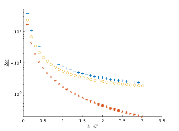
Figure 2: (a )Error in evaluation of glutamate and glycine concentration together by a single receptor, evaluated using Eq.12 represented by ${}^{\prime}*^{\prime}$ and the error evaluated using Eq.9 represented by ${}^{\prime}\circ^{\prime}$ are indeed close as mentioned in the text. Error evaluated using Eq.15 is represented by ${}^{\prime}+^{\prime}$. One can see close agreement with exact error for smaller values of $k_{+}cT$ as expected.(b) Error in measurement of glutamate concentration by the cell as a function of glutamate molecules in a synaptic vesicle. One can see that when this number becomes around $1500$, that the error starts becoming $.5$

Discussion

[24], [25] have considered the problem of limitations to positional measurements in calcium signal transduction. However they considered the kinase concentration to be so high and non changing that the rate equations were considered to be linear. They also didn’t consider the aspect that leads to non-linearities in the problem which arises because calmodulin gets activated only when four $Ca^{2+}$ ions are attached to it. This simplified the form for errors in positional measurement obtained analytically under certain assumptions. We have instead considered non-linearities in these equations and still could make some progress in analytical evaluations as in Eq.15.We saw that Eq.5 were accurate enough in evaluation of error using Eq.9. The reason behind this was that the cytoplasmic rate constants as well as the measurement times colluded to produce order of magnitude concentration values of cytoplasmic reactants as illustrated in Eq.6, leading to the most dominant terms in the rate equations Eq.1, being the first terms on the right hand side. This also led to the error in concentration measurement being independent of the the cytoplasmic rate constants, despite the concentration of cytoplasmic reactants being dependent on them. We should note that it is the order of magnitude of these rate constants and the measurement time and not their absolute values that led to this phenomenon, implying that there was no specific fine tuning of these parameters needed by nature to lead to consistent accuracy in concentration measurement. Since going by [37] we could assume that for both glycine and glutamate the renormalized values of $k_{+}^{glyc}c_{gly}T$ and $k_{+}^{glu}c_{glu}T$ lie $\in[.4,1.7]$. Now, increasing $k_{+}^{glyc}c_{gly}$ and/or $k_{+}^{glu}c_{glu}$ would decrease the error, and since in our calculations we assumed that $k_{+}^{glyc}c_{gly}=k_{+}^{glu}c_{glu}=kc$ and got that the glutamine is accurately detected for $kcT=.4$, we can conclude that for $k_{+}^{glyc}c_{gly}\neq k_{+}^{glu}c_{glu}$ with both $k_{+}^{glyc}c_{gly}T$ and $k_{+}^{glu}c_{glu}T$ lying $\in[.4,1.7]$, the neuron would also accurately detect glutamine concentrations. As can be seen from Fig.2 around $1500$ glutamate molecules per vesicle (calculated using how $k_{+}^{glu}c_{glu}T$ varies with percentage receptor occupancy from Figure.$6$ in [37]) the error in glutamate concentration measurement by the cell becomes around $50$ percent. In regards to error reduction capabilities, we should be concerned with lowest concentration of glutamate measurable by the cell. As stated in [35], in rat brain cortex, number of glutamate molecules per synaptic vesicle was around $1100$ molecules, however $30$ of all the SVs present operate with glutamate as a transmitter, this would raise the number of glutamate molecules per synaptic vesicle to $3640$. We can hence consider that a cell measuring glutamate concentrations upto $50$ percent accuracy for vesicles containing $1500$ molecules to be very apt in measuring glutamate concentrations.

It is always a question as to how various aspects of cellular constructions happened to evolve the way they did. In case of neuronal cells, one could question as to why cells have evolved to be equipped with the specific number of cell surface receptors. As we had mentioned in the introduction, excessive as well as under optimum glutamate concentration in the synaptic cleft would lead to several pathologies[21]. It is hence natural that the neurons should be employed with mechanisms that detect the glutamate concentrations accurately. From our calculations it appears that the way this is accomplished is by using the specifically chosen number of NMDAR receptors on the neuronal surface that accurately detect concentration of glutamate. We have provided evidence as to why nature have chosen the specific number of NMDAR receptors on the surface of the neurons.

Funding

We acknowledge funding from SERB Grant No: EEQ/2021/000006.

Appendix A

We derive how Eq.15 is got in this appendix. We have

$$\langle C_{Pr}\rangle_{n} =\frac{1}{(kc)^{n}}\sum_{Permutate:\tilde{t}_{1},\tilde{t}_{3},\tilde{t}_{5},\tilde{t}_{7}}\int_{\tilde{t}_{1}<\tilde{t}_{3}<\tilde{t}_{5}<\tilde{t}_{7}<kcT}d\tilde{t}_{1}d\tilde{t}_{3}d\tilde{t}_{5}d\tilde{t}_{7}e^{-\tilde{t}_{1}}e^{-\tilde{t}_{3}}e^{-\tilde{t}_{5}}e^{-\tilde{t}_{7}}C(kcT-\tilde{t}_{7})^{n}$$

$$=\frac{4!C}{6(kc)^{n}}\int_{0}^{kcT}e^{-\tilde{t}_{7}}\left(1-e^{-\tilde{t}_{7}}\right)^{3}(kcT-\tilde{t}_{7})^{n}dt_{7}$$

$$=\frac{4!C(kcT)^{n+1}}{6(kc)^{n}}\int_{0}^{1}e^{-kcTx}\left(1-e^{-kcTx}\right)^{3}(1-x)^{n}dx$$

$$=\frac{4!C(kcT)^{n+1}}{6(kc)^{n}}\int_{0}^{1}e^{-kcT}e^{kcTy}\left(1-e^{-kcT}e^{kcTy}\right)^{3}y^{n}dy$$

$$=\frac{4!C(kcT)^{n+1}}{6(kc)^{n}}\int_{0}^{1}e^{kcT(y-1)}\left(1-e^{kcT(y-1)}\right)^{3}y^{n}dy$$

$$=\frac{4!C(kcT)^{n+1}}{6(kc)^{n}}\int_{0}^{1}e^{kcT(y-1)}\left(1-e^{3kcT(y-1)}-3e^{kcT(y-1)}+3e^{2kcT(y-1)}\right)y^{n}dy$$

$$=\frac{4!C(kcT)^{n+1}}{6(kc)^{n}}\int_{0}^{1}\left(e^{kcT(y-1)}-e^{4kcT(y-1)}-3e^{2kcT(y-1)}+3e^{3kcT(y-1)}\right)y^{n}dy$$

Now upto $\mathcal{O}((kcT)^{3})$

$$e^{kcT(y-1)}=1+kcT(y-1)+\frac{(kcT(y-1))^{2}}{2!}+\frac{(kcT(y-1))^{3}}{3!}$$ (17)

$$-e^{4kcT(y-1)}=-1-4kcT(y-1)-\frac{(4kcT(y-1))^{2}}{2!}-\frac{(4kcT(y-1))^{3}}{3!}$$ (18)

$$-3e^{2kcT(y-1)}=-3-6kcT(y-1)-3\frac{(2kcT(y-1))^{2}}{2!}-3\frac{(2kcT(y-1))^{3}}{3!}$$ (19)

$$3e^{3kcT(y-1)}=3+9kcT(y-1)+3\frac{(3kcT(y-1))^{2}}{2!}+3\frac{(3kcT(y-1))^{3}}{3!}$$ (20)

Adding the above four equations gives

$$\left(e^{kcT(y-1)}-e^{4kcT(y-1)}-3e^{2kcT(y-1)}+3e^{3kcT(y-1)}\right)=$$

$$(1-1-3+3)+kcT(y-1)(1-4-6+9)+\frac{(kcT(y-1))^{2}}{2!}(1-16-12+27)$$

$$+\frac{(kcT(y-1))^{3}}{3!}(1-64-24+81)$$

$$=-(kcT(y-1))^{3}$$

$$=(kcT(1-y))^{3}$$

Hence,

$$\langle C_{Pr}\rangle_{n} =\frac{4!C(kcT)^{n+1}}{6(kc)^{n}}\int_{0}^{1}\left(e^{kcT(y-1)}-e^{4kcT(y-1)}-3e^{2kcT(y-1)}+3e^{3kcT(y-1)}\right)y^{n}dy$$

$$=\frac{4!C(kcT)^{n+1}}{6(kc)^{n}}\int_{0}^{1}(kcT(1-y))^{3}*y^{n}dy$$

$$=\frac{4!C(kcT)^{n+4}}{6(kc)^{n}}\int_{0}^{1}(1-y^{3}-3y+3y^{2})*y^{n}dy,\quad kcT<<1$$

$$=\frac{4!C(kcT)^{n+4}}{6(kc)^{n}}\left(\frac{1}{n+1}-\frac{1}{n+4}-\frac{3}{n+2}+\frac{3}{n+3}\right)$$

$$=\frac{4!C(kcT)^{n+4}}{6(kc)^{n}}\left(\frac{n+4-n-1}{(n+1)(n+4)}+\frac{-3n-9+3n+6}{(n+2)(n+3)}\right)$$

$$=\frac{4!C(kcT)^{n+4}}{6(kc)^{n}}\left(\frac{3}{(n+1)(n+4)}-\frac{3}{(n+2)(n+3)}\right)$$

$$=\frac{4!C(kcT)^{n+4}}{2(kc)^{n}}\left(\frac{1}{(n+1)(n+4)}-\frac{1}{(n+2)(n+3)}\right)$$

$$=\frac{4!C(kcT)^{n+4}}{2(kc)^{n}}\left(\frac{(n+2)(n+3)-(n+1)(n+4)}{(n+1)(n+4)(n+2)(n+3)}\right)$$

$$=\frac{4!C(kcT)^{n+4}}{2(kc)^{n}}\left(\frac{n^{2}+5n+6-n^{2}-5n-4}{(n+1)(n+4)(n+2)(n+3)}\right)$$

$$=\frac{4!C(kcT)^{n+4}}{(kc)^{n}(n+1)(n+2)(n+3)(n+4)}$$

Similarly,

$$\langle C_{Pr}^{2}\rangle_{n} =\frac{4!C^{2}(kcT)^{2n+4}}{(kc)^{2n}(2n+1)(2n+2)(2n+3)(2n+4)}$$

Hence

$$\frac{\sqrt{\langle C_{Pr}^{2}\rangle_{n}-\langle C_{Pr}\rangle^{2}_{n}}}{c\frac{d\langle C_{Pr}\rangle_{n}}{dc}}=$$

$$\frac{C*(kcT)^{n+2}}{kc^{n}}\sqrt{\frac{4!}{(2n+1)(2n+2)(2n+3)(2n+4)}-\frac{4!*4!(kcT)^{4}}{(n+1)^{2}(n+2)^{2}(n+3)^{2}(n+4)^{2}}}*$$

$$\frac{(kc)^{n}(n+1)(n+2)(n+3)(n+4)}{4*4!C(kcT)^{n+4}}$$

$$=\sqrt{\frac{4!}{(2n+1)(2n+2)(2n+3)(2n+4)}-\frac{4!*4!(kcT)^{4}}{(n+1)^{2}(n+2)^{2}(n+3)^{2}(n+4)^{2}}}*\frac{(n+1)(n+2)(n+3)(n+4)}{4*4!(kcT)^{2}}$$

$$=\sqrt{\frac{(n+1)^{2}(n+2)^{2}(n+3)^{2}(n+4)^{2}}{4!(2n+1)(2n+2)(2n+3)(2n+4)}-(kcT)^{4}}*\frac{1}{4(kcT)^{2}}$$

$$=\frac{1}{4}\sqrt{\frac{(n+1)^{2}(n+2)^{2}(n+3)^{2}(n+4)^{2}}{4!(kcT)^{4}(2n+1)(2n+2)(2n+3)(2n+4)}-1}$$

$$=\frac{1}{4}\sqrt{\frac{(n+1)(n+2)(n+3)^{2}(n+4)^{2}}{4!4(kcT)^{4}(2n+1)(2n+3)}-1}$$

“Data Availability Statement

There is no data associated with this manuscript.

Author contribution statement

Both authors contributed equally to the manuscript

References

- [1] Mao, H., Cremer, P. S., Manson, M. D. (2003). A sensitive, versatile microfluidic assay for bacterial chemotaxis. Proceedings of the National Academy of Sciences, 100(9), 5449-5454.
- [2] Endres, R. G., Wingreen, N. S. (2009). Maximum likelihood and the single receptor. Physical review letters, 103(15), 158101.
- [3] Rieke, F., Baylor, D. A. (1998). Single-photon detection by rod cells of the retina. Reviews of Modern Physics, 70(3), 1027.
- [4] Segall, J. E. (1993). Polarization of yeast cells in spatial gradients of alpha mating factor. Proceedings of the National Academy of Sciences, 90(18), 8332-8336.
- [5] Rappel, W. J., Levine, H. (2008). Receptor noise limitations on chemotactic sensing. Proceedings of the National Academy of Sciences, 105(49), 19270-19275.
- [6] Ueda, M., Shibata, T. (2007). Stochastic signal processing and transduction in chemotactic response of eukaryotic cells. Biophysical journal, 93(1), 11-20.
- [7] B. Alberts, A. Johnson, J. Lewis, M. Raff, K. Roberts, P. Walter, Molecular Biology of the Cell, 5th ed. edited by B. Alberts (Garland Science, Oxford, 2008).
- [8] Berg, H. C., Purcell, E. M. (1977). Physics of chemoreception. Biophysical journal, 20(2), 193-219.
- [9] Bialek, W., Setayeshgar, S. (2005). Physical limits to biochemical signaling. Proceedings of the National Academy of Sciences, 102(29), 10040-10045.
- [10] Wang, K., Rappel, W. J., Kerr, R., Levine, H. (2007). Quantifying noise levels of intercellular signals. Physical Review E, 75(6), 061905.
- [11] Mora, T., Wingreen, N. S. (2010). Limits of sensing temporal concentration changes by single cells. Physical review letters, 104(24), 248101.
- [12] Fancher, S., Mugler, A. (2017). Fundamental limits to collective concentration sensing in cell populations. Physical review letters, 118(7), 078101.
- [13] Hu B, Chen W, Rappel WJ, Levine H. 2010. Physical limits on cellular sensing of spatial gradients.
- [14] Wasnik, V. (2022). Limitations on concentration measurements and gradient discerning times in cellular systems. Physical Review E, 105(3), 034410.
- [15] Endres, R. G., Wingreen, N. S. (2008). Accuracy of direct gradient sensing by single cells. Proceedings of the National Academy of Sciences, 105(41), 15749-15754.
- [16] Mugler, A., Levchenko, A., Nemenman, I. (2016). Limits to the precision of gradient sensing with spatial communication and temporal integration. Proceedings of the National Academy of Sciences, 113(6), E689-E695.
- [17] D. Ellison, A. Mugler, M. D. Brennan, S. H. Lee, R. J. Huebner, E. R. Shamir, L. A. Woo, J. Kim, P. Amar, I. Nemenman, A. J. Ewald, and A. Levchenko, Proc. Natl. Acad. Sci. U.S.A. 113, E679 (2016).
- [18] B. W. Andrews and P. A. Iglesias, PLoS Comput. Biol. 3, e153 (2007).
- [19] B. Hu, W. Chen, W.-J. Rappel, and H. Levine, Phys. Rev. Lett. 105, 048104 (2010).
- [20] F. Tostevin, P. R. ten Wolde, and M. Howard, PLoS Comput. Biol. 3, e78 (2007).
- [21] Murrough, J. W., Abdallah, C. G., Mathew, S. J. (2017). Targeting glutamate signalling in depression: progress and prospects. Nature Reviews Drug Discovery, 16(7), 472-486.
- [22] T.D. Lamb, (1996). Gain and kinetics of activation in the G-protein cascade of phototransduction Proc. Natl. Acad. Sci. U.S.A., 93 pp. 566-570
- [23] M.C. Gustin, J. Albertyn, M. Alexander, K. Davenport. (1998), MAP kinase pathways in the yeast Saccharomyces cervisiae Microbiol. Mol. Biol. Rev., 62 pp. 1264-1300
- [24] Wasnik, V. H., Lipp, P., Kruse, K. (2019). Accuracy of position determination in Ca 2+ signaling. Physical Review E, 100(2), 022401.
- [25] Wasnik, V. H., Lipp, P., Kruse, K. (2019). Positional Information Readout in Ca 2+ Signaling. Physical review letters, 123(5), 058102.
- [26] Seger R, Krebs EG. The MAPK signaling cascade. FASEB J. 1995 Jun;9(9):726-35. PMID: 7601337.
- [27] P.B. Detwiler, S. Ramanathan, A. Sengupta, B. Shraiman. (2000), Engineering aspects of enzymatic signal transduction: photoreceptors in the retina Biophys. J., 79 pp. 2801-2817
- [28] Thattai, M., van Oudenaarden, A. (2002). Attenuation of noise in ultrasensitive signaling cascades. Biophysical journal, 82(6), 2943-2950.
- [29] Shibata, T., Fujimoto, K. (2005). Noisy signal amplification in ultrasensitive signal transduction. Proceedings of the National Academy of Sciences, 102(2), 331-336.
- [30] Tănase-Nicola, S., Warren, P. B., Ten Wolde, P. R. (2006). Signal detection, modularity, and the correlation between extrinsic and intrinsic noise in biochemical networks. Physical review letters, 97(6), 068102.
- [31] Bruggeman, F. J., Blüthgen, N., Westerhoff, H. V. (2009). Noise management by molecular networks. PLoS computational biology, 5(9), e1000506.
- [32] Hooshangi, S., Thiberge, S., Weiss, R. (2005). Ultrasensitivity and noise propagation in a synthetic transcriptional cascade. Proceedings of the National Academy of Sciences, 102(10), 3581-3586.
- [33] . Franks KM, Bartol TM, Sejnowski TJ (2002) A Monte Carlo model reveals independent signaling at central glutamatergic synapses. Biophys J 83: 2333–2348.
- [34] Budisantoso T, Harada H, Kamasawa N, Fukazawa Y, Shigemoto R, Matsui K. Evaluation of glutamate concentration transient in the synaptic cleft of the rat calyx of Held. J Physiol. 2013 Jan 1;591(1):219-39. doi: 10.1113/jphysiol.2012.241398. Epub 2012 Oct 15. PMID: 23070699; PMCID: PMC3630782.
- [35] Riveros, N., J. Fiedler, N. Lagos, C. Munoz, and F. Orrego. 1986. Gluta- mate in rat brain cortex synaptic vesicles: influence of the vesicle isolation procedure. Brain Res. 386:405-408.
- [36] Timothy A. Ryan, Harald Reuter, Beverly Wendland, Felix E. Schweizer, Richard W. Tsien, Stephen J. Smith, The kinetics of synaptic vesicle recycling measured at single presynaptic boutons, Neuron, Volume 11, Issue 4, 1993, Pages 713-724, ISSN 0896-6273
- [37] Holmes, W. R. (1995). Modeling the effect of glutamate diffusion and uptake on NMDA and non-NMDA receptor saturation. Biophysical Journal, 69(5), 1734-1747.
- [38] Johnson JW, Ascher P. Equilibrium and kinetic study of glycine action on the N-methyl-D-aspartate receptor in cultured mouse brain neurons. J Physiol. 1992 Sep;455:339-65. doi: 10.1113/jphysiol.1992.sp019305. PMID: 1484357; PMCID: PMC1175648.
- [39] Clapham, D. E. (2007). Calcium signaling. Cell, 131(6), 1047-1058.
- [40] Cottrell, J. R., Dube, G. R., Egles, C., Liu, G. (2000). Distribution, density, and clustering of functional glutamate receptors before and after synaptogenesis in hippocampal neurons. Journal of neurophysiology, 84(3), 1573-1587.
- [41] M.J. Berridge, P. Lipp, M.D. Bootman The versatility and universality of calcium signalling Nat. Rev. Mol. Cell Biol., 1 (2000), pp. 11-21
- [42] Saucerman, J. J., Bers, D. M. (2008). Calmodulin mediates differential sensitivity of CaMKII and calcineurin to local Ca2+ in cardiac myocytes. Biophysical journal, 95(10), 4597-4612.
- [43] Timofeeva, Y., Volynski, K. (2015). Calmodulin as a major calcium buffer shaping vesicular release and short-term synaptic plasticity: facilitation through buffer dislocation. Frontiers in cellular neuroscience, 9, 239.
- [44] Keller, D. X., Franks, K. M., Bartol Jr, T. M., Sejnowski, T. J. (2008). Calmodulin activation by calcium transients in the postsynaptic density of dendritic spines. PloS one, 3(4), e2045.