Recent Applications of Dynamical Mean-Field Methods

Abstract

Rich out of equilibrium collective dynamics of strongly interacting large assemblies emerge in many areas of science. Some intriguing and not fully understood examples are the glassy arrest in atomic, molecular or colloidal systems, flocking in natural or artificial active matter, and the organization and subsistence of ecosystems. The learning process, and ensuing amazing performance, of deep neural networks bears resemblance with some of the before-mentioned examples. Quantum mechanical extensions are also of interest. In exact or approximate manner the evolution of these systems can be expressed in terms of a dynamical mean-field theory which not only captures many of their peculiar effects but also has predictive power. This short review presents a summary of recent developments of this approach with emphasis on applications on the examples mentioned above.

1 INTRODUCTION

In condensed matter or statistical physics focus is set on macroscopic systems in thermal equilibrium. The relaxation of a tiny perturbation away from equilibrium is also sometimes described in textbooks and undergraduate courses. However, the vast majority of physical systems evolve far from equilibrium.

Take a classical macroscopic physical system in conventional equilibrium. Any change in the properties of the environment in a canonical setting, or in the system’s Hamiltonian itself in a microcanonical one, will take it away from equilibrium. The procedure of rapidly (ideally instantaneously) tuning a parameter is called a quench. The post-quench relaxation towards the new equilibrium (if possible) could be fast or very slow, and even need a time scaling with the system size. Well-known cases include systems quenched to a critical point [1] or across a second order phase transition [2, 3, 4, 5]. Less well-understood cases, as those with competing interactions that behave as glasses have exceedingly long relaxations as well [6]. The post-quench dynamics of closed systems are also of great interest at present, boosted by cold atom experiments performed in almost perfect isolation [7].

Out of equilibrium situations can also be established by external drives. In the context of macroscopic physics, a traditional example is Rayleigh-Bénard convection induced in a layer of fluid by two parallel confining plates maintained at different temperatures. Another appealing instance is the one of powders stuck in static metastable states unless tapping, vibration or shear make them slowly evolve towards more compact configurations [8]. Active matter, with manifold physical, biological and artificial realizations is another example, in which energy is injected at the microscopic constituent level [9].

The out of equilibrium evolution of systems with many interacting components is not restricted to physics. Celebrated areas in which tools learnt and developed to deal with complex physical systems are currently being applied with success are theoretical ecology [10], neuroscience [11], computer science [12], and econophysics [13], to name just a few.

The problems discussed in the previous paragraphs pertain to the classical World. In other cases of practical interest, quantum fluctuations play an important rôle. The main focus of this review will be the description of classical non-equilibrium dynamics, but we will comment on applications of highlighted notions to quantum ones as well.

Characterizing the macroscopic behavior of far from equilibrium systems is challenging. One cannot rely on any ergodic hypothesis to compute statistical averages and, in contrast, full time dependencies have to be elucidated. Much inspiration has been gained from the study of simplified microscopic models that do capture important features of coarsening, glassy and weakly driven systems. These approximate mathematical representations are often bona fide ones for problems in other, and at least as interesting, areas of science. We present a set of models that have been key to the construction of quite a general picture for the non-equilibrium dynamics of complex systems with slow dynamics in Sec. 2. The review goes on with the recollection of methods and ideas developed in the study of their relaxational dynamics in Secs. 3, 4, and 5. We then focus on recent applications and discoveries. In Sec. 6 we describe the peculiarities of their Hamiltonian evolution. Section 7 is devoted to the discussion of cases explicitly maintained far from equilibrium by the action of non-potential forces. Applications to active matter and ecology pertain to this class. We also comment of recent progress in the analysis of stochastic learning processes of neural networks. In relaxational cases, rough free-energy landscapes play a crucial role in trapping the dynamics. In the driven ones the complexity translates to the random forces. Finally, we briefly discuss quantum extensions and relations to recent work in high-energy physics in Sec. 8. We close with conclusions and some open problems in Sec. 9. Several lecture notes and review articles give a more technical presentation of the formalism discussed here. The reader interested in learning the mathematical derivations can consult Refs. [14, 15, 16, 17].

2 MODELS

Consider the set of coupled differential equations

$$m\frac{d^{2}x_{i}(t)}{dt^{2}}+\eta\frac{dx_{i}(t)}{dt}=g_{i}(x_{i})+f_{i}(x_{1},\dots,x_{N})+h_{i}(t)+\xi_{i}(t)\;,$$ (1)

ruling the time dependence of a typically large number of real-valued variables $x_{i}(t)$, $i=1,\dots,N$. In their simplest interpretation, these variables represent the Cartesian coordinates of the position vector $\vec{x}=(x_{1},\dots,x_{N})$ of a point-like particle with mass $m$ moving in an $N$-dimensional space. The space of configurations is continuous and differentiable.

The inertial term in the left-hand-side is important to model Hamiltonian dynamics as well as to establish quantum extensions. In the Langevin case it gives rise to under-damped dynamics, while when negligible the dynamics get over-damped.

The last term in the right-hand-side is a white Gaussian thermal noise with

$$\langle\xi_{i}(t)\rangle=0\;,\qquad\qquad\langle\xi_{i}(t)\xi_{j}(t^{\prime})\rangle=2\eta k_{B}T\,\delta_{ij}\delta(t-t^{\prime})\;,$$ (2)

which, together with the friction terms $\eta\dot{x}_{i}$ model the coupling of $x_{i}$ to an equilibrated bath at temperature $T$. The coupling strength is controlled by the friction coefficient $\eta$. The balance between the noise correlation and friction kernel ensures that the environment is in thermal equilibrium. Henceforth, noise averages are indicated with angular brackets $\langle\dots\rangle$.

The coupling to colored baths which are not necessarily in equilibrium could also be used. For still Gaussian noises, the friction term and noise-noise correlations generalize to

$$\int_{0}^{t}dt^{\prime}\;\Gamma_{R}(t,t^{\prime})\,\frac{dx_{i}(t^{\prime})}{dt^{\prime}}\;,\qquad\qquad\qquad\langle\xi_{i}(t)\xi_{j}(t^{\prime})\rangle=\delta_{ij}\,\Gamma_{C}(t,t^{\prime})\;.$$ (3)

The kernels satisfy $\Gamma_{R}(t,t^{\prime})\propto\theta(t-t^{\prime})$ (causality) and $\Gamma_{C}(t,t^{\prime})=\Gamma_{C}(t^{\prime},t)$ (symmetry) and represent the linear response and correlation of the bath. In equilibrium both kernels are time-translationally invariant, meaning that they only depend on time-difference $t-t^{\prime}$. A fluctuation-dissipation-theorem (FDT) holds: $\Gamma_{C}(t-t^{\prime})=k_{B}T\,[\Gamma_{R}(t-t^{\prime})+\Gamma_{R}(t^{\prime}-t)]$ or equivalently $\Gamma_{R}(t-t^{\prime})=\beta\theta(t-t^{\prime})\Gamma_{C}(t-t^{\prime})$. Equilibrium white noise is recovered with $\Gamma_{C}(t-t^{\prime})=k_{B}T\,\eta/\tau\,e^{-|t-t^{\prime}|/\tau}$ and $\Gamma_{R}(t-t^{\prime})=\eta/\tau\,e^{-|t-t^{\prime}|/\tau}\theta(t-t^{\prime})$ in the limit in which the characteristic time vanishes, $\tau\to 0$, implying $\Gamma_{C}(t-t^{\prime})\to 2\eta k_{B}T\,\delta(t-t^{\prime})$ and $\Gamma_{R}(t-t^{\prime})\to 2\eta\delta(t-t^{\prime})\theta(t-t^{\prime})$. Some active matter models use this last $\Gamma_{R}(t-t^{\prime})$ with $\Gamma_{C}(t-t^{\prime})=2\eta k_{B}T\,\delta(t-t^{\prime})+\Gamma_{\rm act}(t-t^{\prime})$, where $\Gamma_{\rm act}(t-t^{\prime})$ is interpreted as being due to particle self-propulsion and violates FDT by construction.

We will mostly use equilibrium white noise. The coupling to the environment can then be on by keeping $\eta\neq 0$ or switched off by setting $\eta=0$. The noise can be eliminated by putting $T$ to zero, rendering the stochastic Langevin Equations 1 deterministic.

The time-dependent functions $h_{i}(t)$ are external forces. They can be, for example, sinusoidal, $h_{i}(t)=h\sin(\omega t)$, and relevant to discuss periodically driven systems, or just constant as in an infinitesimal perturbation applied to measure a linear response.

The term $g_{i}(x_{i})$ is a local force which could restrict the values of $x_{i}$ for $g_{i}(x_{i})=-V_{i}^{\prime}(x_{i})$ with $V_{i}(x_{i})=u(x^{2}_{i}-a^{2}_{i})^{2}$ and favor $x_{i}=\pm a_{i}$, or it could impose a global spherical constraint

$$\sum_{i=1}^{N}x_{i}^{2}=N\qquad\Rightarrow\qquad g_{i}(x_{i})=z(t)x_{i}\;,$$ (4)

(on average) with the Lagrange multiplier $z(t)$ to be determined self-consistently. In this case, the particle is forced to move on the sphere of radius $N^{1/2}$ and $\langle\vec{x}\cdot\frac{d\vec{x}}{dt}\rangle=0$.

[] Fully-connectedEach variable interacts with all others. The internal forces $f_{i}(x_{1},\dots,x_{N})$ are generically multi-body. We will concentrate on fully-connected models, such that each variable interacts with all other ones, and the forces are independent of any distance. Moreover, we will consider disordered $f_{i}$, which depend on quenched random parameters drawn from a time-independent probability distribution. [] Quenched disorderTime-independent parameters drawn from a probability distribution.

Whenever the forces are conservative, $f_{i}=-\partial V/\partial x_{i}$, we focus on a Gaussian distributed potential energy $V$ with $[V(\vec{x})]=0$ and $[V(\vec{x})V(\vec{y})]=N\;\widetilde{V}\left(|\vec{x}-\vec{y}|^{2}/N\right)$. [] Conservative forcesThose that derive from a potential energy. Henceforth, $[\dots]$ denote average over disorder. The scaling with $N$ ensures an interesting thermodynamic limit. For notational simplicity and also to ease the understanding, we collect all $x_{i}$ in the $N$ dimensional vector $\vec{x}=(x_{1},\dots,x_{N})$.

The $p$-spin models, originally proposed for Ising variables [18] but later generalized to spherical ones [19],

$$V(\vec{x})=-\sum_{i_{1}<\dots<i_{p}}\!\!\!J_{i_{1}\dots i_{p}}x_{i_{1}}\dots x_{i_{p}}\;,$$ (5)

with a fixed integer, $p\geq 2$, belong to this category. The couplings $J_{i_{1}\dots i_{p}}$, symmetric under the permutation of any pair of indices, are i.i.d. quenched random variables Gaussian distributed with $[J_{i_{1}\dots i_{p}}]=0$, $[J_{i_{1}\dots i_{p}}^{2}]=p!J^{2}/(2N^{p-1})$, and uncorrelated for different sets of indices. The potential energy correlation then reduces to

$$[V(\vec{x})V(\vec{y})]=N\;\overline{V}(\vec{x}\cdot\vec{y}/N)\qquad\mbox{with}\qquad\overline{V}(q)=(J^{2}/2)\,q^{p}\;.$$ (6)

At zero temperature ($T=0$), vanishing external forces ($h_{i}=0$), and in the absence of the inertial term ($\eta/m\gg 1$), the potential dynamics boil down to a gradient descent. Switching off the coupling to the bath ($\eta=0$), the sum of kinetic and potential energies is conserved. For special $V$ there can be other conserved quantities and even as many as the number of degrees of freedom, making the dynamics integrable (see Sec. 6).

Non-reciprocal forces do not satisfy Newton’s action-reaction principle. Simple extensions of the model defined in Equation 5 provide examples of this kind; e.g., [] Non-reciprocal forcesthose that violate the action-reaction principle.

$$f_{i}(\vec{x})=(\sum_{(i<)j_{2}<\dots<j_{p}}+\sum_{j_{2}(<i<)j_{3}<\dots<j_{p}}+\dots+\sum_{j_{2}<\dots<j_{p}(<i)})\;J_{ij_{2}\dots j_{p}}x_{j_{2}}\dots x_{j_{p}}\;,$$ (7)

where each constrained multi-sum runs over $p-1$ indices, if the exchanges $J_{ij_{2}\dots j_{p}}$ are symmetric under permutations of the $j_{2},\dots,j_{p}$ indices but they are not under permutations of the index $i$ with any of the $j$s [20, 21, 22, 23] (see Sec. 7). They have zero mean, are uncorrelated for different indices, and have variance $p!/(2N^{p-1})$. Then, $[f_{i}(\vec{x})]=0$ and

$$[f_{i}(\vec{x})f_{j}(\vec{y})] = \delta_{ij}\;N\,\overline{V}^{\prime}\left(\frac{\vec{x}\cdot\vec{y}}{N}\right)+x_{j}y_{i}\;\overline{V}^{\prime\prime}\left(\frac{\vec{x}\cdot\vec{y}}{N}\right)+(\gamma-1)\,x_{j}y_{i}\;\overline{V}^{\prime\prime}\left(\frac{\vec{x}\cdot\vec{y}}{N}\right)\;.$$ (8)

The conservative case is recovered for $\gamma=1$.

The dynamics are usually studied on average over initial conditions $\{x_{i}(0),\,\dot{x}_{i}(0)\}$ sampled from distributions which reflect specific situations, like thermal equilibrium at a prescribed temperature, or knowledge of the forces $f_{i}$. Preparing initial conditions in canonical equilibrium at $\beta_{0}$ and evolving them with Langevin dynamics at $\beta$ is one way to perform a quench. Notation-wise, when there is thermal noise, we include the average over initial conditions in $\langle\dots\rangle$ while for deterministic dynamics we denote it $\langle\dots\rangle_{i.c.}$. [] QuenchA sudden change in a control parameter that sets the system out of equilibrium.

This set of equations has sufficient ingredients to encompass, at least at some level of approximation, a large number of many-body physical phenomena, including the ones listed as examples in the Introduction. Furthermore, they also mimic problems in other areas of science, such as neural networks [11], optimization and computer science [12], evolution and game theory [24] or even markets [13]. Because of the complicated nature of the $f_{i}$, these problems are dubbed complex systems. In interesting cases the interactions are strong and perturbative methods fail badly; self-consistent approaches, as the ones discussed in Sec. 3, are better suited to deal with them. Quantum extensions (Sec. 8) have been considered in the statistical physics literature and have also become fashionable among high-energy physicists since the Sachdev-Ye-Kitaev (SYK) model, a fermionic analog of the classical $p$ body model, is a toy model of holography.

3 DYNAMICAL MEAN-FIELD METHODS

There are two alternative ways to exploit the fully-connected character of the models at hand, and write manageable equations for their evolution. One way derives deterministic coupled integro-differential equations for correlation and linear response functions of Schwinger-Dyson kind. The other represents the full dynamics with an effective non-Markov Langevin equation for a single degree of freedom. We schematically present them here.

3.1 Schwinger-Dyson equations

In the $N\to\infty$ limit the dynamics of the spherical models are fully characterized by the two-time global correlation and linear response. The equations ruling their evolution can be derived with the Martin-Siggia-Rose-Jansen-DeDominicis (MSRJD) functional formalism [25, 26, 27, 28] [] MSRJD The functional integral generating function of Langevin processes. or with perturbative methods combined with self-consistent diagram re-summation [29]. A common choice is to weight the initial conditions with the Gibbs-Boltzmann measure

$$P(\{x_{i}(0),\dot{x}_{i}(0)\})=Z^{-1}(\beta_{0})\,{\rm e}^{-\beta_{0}H_{0}(\{x_{i}(0),\dot{x}_{i}(0))\}}$$ (9)

at temperature $T_{0}$ with $H_{0}$ the pre-quench Hamiltonian. For $T_{0}^{-1}=\beta_{0}\to 0$ they are completely random while for $\beta_{0}>0$ they have knowledge of the Hamiltonian $H_{0}$. (Hereafter we measure $T$ in units of $k_{B}$.) In order to average over them, when $H_{0}$ depends on quenched random parameters, one resorts to the replica method [18]. [] Replica method A technique to compute the disorder averaged free-energy. When the quench concerns a change in temperature but not in the Hamiltonian, or it consists in a global rescaling of the random coupling strengths, the replica structure of the initial conditions, which depends on $\beta_{0}$ and $H_{0}$, is conserved in time. Choosing, for simplicity, $T_{0}\geq T^{0}_{s}$, the static critical temperature of the model $H_{0}$, the replica structure is rather simple (symmetric) and the dynamics can then be fully encoded in the two-time correlation and linear response:

$$C(t_{1},t_{2})=N^{-1}\sum_{i=1}^{N}\;[\langle x_{i}(t_{1})x_{i}(t_{2})\rangle]\;,\qquad\quad R(t_{1},t_{2})=\left.N^{-1}\sum_{i=1}^{N}\;[\langle\frac{\delta{x}^{(h)}_{i}(t_{1})}{\delta h_{i}(t_{2})}\rangle]\right|_{h=0}\!\!\!\!\!\!\!\!\!\!\;,\;\;\;$$ (10)

for $t_{1},\ t_{2}>0$, where $\vec{x}$ represents any of the replicas, as they are all equivalent. The infinitesimal perturbation $\vec{h}$ is coupled linearly to the $x_{i}$ according to $H\mapsto H-\sum_{i=1}^{N}h_{i}x_{i}$ at time $t_{2}$ and the upper-script ${(h)}$ indicates that the configuration is measured under the field $\vec{h}$. The boundary values of $C$ and $R$ at $t_{1}=t_{2}$ depend on whether the inertia term is present and whether the system is open or closed. Naming $z(t_{1})$ is the Lagrange multiplier which enforces the spherical constraint $C(t_{1},t_{1})=1$, using an homogeneous external field $h(t)$, and calling

$$G_{0}^{-1}(t_{1})=m\partial_{t_{1}}^{2}+\eta\partial_{t_{1}}+z(t_{1})\;,$$ (11)

the Schwinger-Dyson equations read [30, 31, 32, 33, 34] [] Schwinger-Dyson equations Closed integro-differential equations for correlations and linear responses.

$$G_{0}^{-1}(t_{1})R(t_{1},t_{2})=\delta(t_{1}-t_{2})+\int_{t_{2}}^{t_{1}}dt\;\Sigma(t_{1},t)R(t,t_{2})\;,$$ (12)

$$G_{0}^{-1}(t_{1})C(t_{1},t_{2})=\int_{0}^{t_{1}}dt\;\Sigma(t_{1},t)C(t,t_{2})+\int_{0}^{t_{2}}dt\;D(t_{1},t)R(t_{2},t)+\;\eta TR(t_{2},t_{1})$$

$$\qquad\qquad\qquad\qquad+\,h(t_{1})\int_{0}^{t_{2}}dt\;h(t)R(t_{2},t)+\beta_{0}D(t_{1},0)C(t_{2},0)\;,\;$$ (13)

$$z(t_{1})=\int_{0}^{t_{1}}dt\;[\Sigma(t_{1},t)C(t_{1},t)+D(t_{1},t)R(t_{1},t)]-m\partial_{t_{1}}^{2}C(t_{1},t_{2})|_{t_{2}\rightarrow t_{1}^{-}}$$

$$\qquad\quad+\eta TR(t_{2}\to t^{-}_{1},t_{1})+h(t_{1})\int_{0}^{t_{1}}\!dt\,h(t)R(t_{1},t)+\beta_{0}D(t_{1},0)C(t_{1},0)\;.$$ (14)

The self-energy and vertex kernels, $\Sigma$ and $D$, depend on the correlation of the forces $f_{i}$,

$$\Sigma=\overline{V}^{\prime\prime}\!(C)R\qquad{\rm and}\qquad D=\overline{V}^{\prime}(C)\qquad\Rightarrow\qquad\Sigma=D^{\prime}R$$ (15)

for the potential cases in Equation 8. The terms proportional to $J_{0}/T_{0}$ impose the initial conditions. Importantly enough, out of equilibrium the linear response and correlation function are not necessarily related to one another and the equilibrium fluctuation dissipation theorem

$$T\,R(t_{1},t_{2})=\frac{\partial}{\partial t_{2}}C(t_{1},t_{2})\,\qquad\mbox{for}\;\;t_{1}\geq t_{2}\qquad\qquad{\mbox{(FDT)}}$$ (16)

does not need to hold. Each two-time function should be determined independently. [] FDT A model independent relation between linear response and correlation functions valid in equilibrium.

In quantum models one can proceed similarly, using the closed-time-path or Schwinger-Keldysh path integral [35, 36] formalism and derive the corresponding Schwinger-Dyson equations. This can be done even for special choices of initial states, as the canonical equilibrium ones [37, 34, 38].

3.2 Single variable effective representation

An alternative method allows one to analyze the dynamics of interacting degrees of freedom in terms of a self-consistent one-body problem. The single variable effective Langevin equation can be derived from the MSRJD dynamic generating functional averaged over the quenched randomness [30, 31, 39] [] Single variable effective description The self-consistent one-body problem.

$$G_{0}^{-1}(t_{1})x(t_{1})+\int_{0}^{t_{1}}dt^{\prime}\;\tilde{\Sigma}(t_{1},t^{\prime})x(t^{\prime})=\beta_{0}\tilde{D}(t_{1},0)x(0)+h(t_{1})+\zeta(t_{1})+\xi(t_{1})\;.$$ (17)

The representative variable is $x$ and $G_{0}^{-1}$ is the differential operator defined in Equation 11. There are two uncorrelated noises: the original zero-average white noise $\xi$, and a new effective noise $\zeta$, also with zero mean and

$$\langle\zeta(t_{1})\zeta(t_{2})\rangle=\tilde{D}(t_{1},t_{2})\;.$$ (18)

The vertex $\tilde{D}$ acts as the colored noise correlation and the self-energy $\tilde{\Sigma}$ as the time-derivative of a retarded friction in the non-Markovian Langevin Equation 17. In the potential case they take the same functional forms as in Equation 15 with

$$\tilde{C}(t_{1},t_{2})=x(t_{1})x(t_{2})\;,\qquad\qquad\quad\tilde{R}(t_{1},t_{2})=\left.\frac{\delta x(t_{1})}{\delta h(t_{2})}\right|_{h=0}\!\!\!\!$$ (19)

and they collect the effects of the other degrees of freedom on the selected one. Note that $\tilde{C}$ and $\tilde{R}$ are not averaged over the thermal noises but in the $N\to\infty$ limit the fluctuations should be suppressed [40], and $\langle\tilde{C}\rangle\to C$ and $\langle\tilde{R}\rangle\to R$, where the angular brackets represent an average over both $\xi$ and $\zeta$. The global spherical constraint transforms in $\langle x^{2}(t)\rangle=1$. The set of equations has to be solved self-consistently; the difficulty lies in imposing the condition 18.

The single variable equation can also be derived with an extension of the static cavity method to the time-dependent problem [18, 39, 41]. This technique is particularly useful since it allows one to treat problems with non-linear $g_{i}(x_{i})$, and find that the linear term $z(t_{1})x(t_{1})$ is replaced by $g^{\prime}_{i}(x_{i})$ and, also, “noise multiplicative” cases, as the ecological models of Sec. 7.2. The analysis in [39] gives a very detailed explanation of how to sample $x(0)$ and $\zeta(0)$ so as to comply with equilibrium conditions at $\beta_{0}$. [] Cavity method a generalization of the Bethe—Peierls iterative technique used to obtain the static properties of models defined on tree-like graphs.

This approach bears similarity to the Dynamical Mean-Field Theory [42] which has been so successfully applied to condensed matter systems, though mostly in equilibrium.

4 RUGGED FREE-ENERGY LANDSCAPES

In potential cases, the Thouless-Anderson-Palmer (TAP) free-energy landscape [18] that generalizes the Ginzburg-Landau one to cases with $N$ order parameters can be constructed and studied in great detail, see Refs. [43, 44] for recent reviews. In order to set the stage for the discussion of the relaxation of conservative systems we briefly recall their main features. [] TAP free-energy landscapeAn extension of the Ginzburg-Landau free-energy to cases with $N$ local order parameters.

4.1 The spherical $p=2$ case

The spherically constrained random harmonic potential is still complex enough to allow for an equilibrium phase transition [45] but the structure of the free-energy landscape is rather simple. There are only two equilibrium states at $T<T_{s}$ related by $x_{i}\mapsto-x_{i}$ for all $i$, akin to a conventional second order phase transition with spontaneous symmetry breaking. The ground states are $\vec{x}=\pm\vec{v}^{\;\rm max}=\pm\vec{v}_{\mu=N}$, the eigenvector associated to the largest (ordered so that $\mu=N$) eigenvalue of the GOE coupling matrix ${\mathbb{J}}$. The equilibrium states at $T<T_{s}$ just dress these configurations with thermal fluctuations, see the sketch in Fig. 1(b). The configurations closely aligned with the other eigenvectors of ${\mathbb{J}}$ belong to metastable states. They are ordered according to their stability and energy, with the maximum associated to the eigenvector with the lowest eigenvalue ($\mu=1$). Under a constant and uniform field $\vec{h}$ the number of stationary points of the potential energy is reduced to just two with one of the zero-field ground states being selected by the field. There is no finite temperature phase transition under a field.

Under spontaneous symmetry breaking, $\langle x_{\mu=N}\rangle_{\rm eq}\equiv\langle\vec{x}\cdot\vec{v}_{N}\rangle_{\rm eq}=(q_{\rm EA}N)^{1/2}$ and one mode is macroscopically occupied until $T_{s}$ where $q_{\rm EA}$ vanishes. This special alignment resembles Bose-Einstein condensation and for this reason one calls the equilibrium low-temperature configurations condensed and the high temperature ones extended.

Within replica theory, this model is replica symmetric (RS) since the Parisi overlap matrix, ${\mathbb{Q}}=(Q_{ab}=N^{-1}\sum_{i}[\langle x_{i}^{a}x_{i}^{b}\rangle])$, is filled with identical values $Q_{a\neq b}=q_{\rm EA}$. The parameter $q_{\rm EA}$ quantifies the “size” of the equilibrium states.

4.2 The Sherrington-Kirkpatrick model

In the Sherrington-Kirkpatrick model of spins glasses, $p=2$ and $x_{i}=\pm 1$, there is a phase transition at $T_{s}$. The replica structure at $T<T_{s}$ needs a full replica symmetry breaking (FRSB) and this entails a hierarchical (ultrametric) organization of equilibrium states as the one in Fig. 2(c). In a few words, there are equilibrium states of all kinds, in the sense that the overlap between two configurations in equilibrium can take any value $0\leq q<q_{\rm EA}$. Barriers between them and the metastable states scale sub-linearly with $N$ [18].

4.3 The spherical $p\geq 3$ potentials

The spherical $p\geq 3$ models, defined by the potential energy in Equation 5, belong to a different universality class from all points of view (static, landscape, and dynamic). Their TAP free-energy landscape is complex [46, 47, 48, 49, 50, 51] with manifold consequences.

1. For $T>T_{d}$ there is a single global minimum, with vanishing local order parameters, $\langle x_{i}\rangle=0$ (paramagnetic/liquid). Any two typical configurations in equilibrium at these temperatures are orthogonal. (Sketch in Fig. 1(a) and Fig. 2(a).) [] ComplexityThe logarithm of the number of stationary points of the TAP free-energy landscape.

2. In the interval $T_{s}<T<T_{d}$ there is ergodicity breaking with an exponentially large number of (metastable) states, that is, a finite complexity, defined as the logarithm of the number of such states (also called configurational entropy). Metastable states are sets of configurations separated by free-energy barriers whose height scale as $N$. The averages of the $x_{i}$ over all configurations belonging to the same state are the $N$ order parameters, $\langle x_{i}\rangle\neq 0$. The stable states are in one-to-one correspondence with local minima of the potential energy. They can be followed in temperature until a spinodal where they disappear without crossing, merging nor dividing [47]. Two configurations from the same state have finite overlap $q_{1}$ while two configurations from different states are orthogonal and have vanishing overlap $q_{0}=0$ (sketches in Fig. 1(c) and 2(b)). In spite of the existence of so many metastable states in this range of temperatures, the equilibrium properties are the simple continuation of the high temperature ones. Their behavior at $T\stackrel{{\scriptstyle>}}{{\sim}}T_{d}$ is like the one of super-cooled liquids [52].

3. For $T<T_{s}$ the lowest lying states dominate the equilibrium measure, and have zero complexity (entropy crisis). This drives the static glass transition, which is thermodynamically second order (the energy is continuous and there is no latent heat), but the global order parameter is discontinuous and jumps to a finite value as in a first order transition. This entropy vanishing transition, is the analog of the empirically-defined Kauzmann transition, where a crossing of the configurational entropy of the crystal and the glass is envisioned to occur in real materials [53]. The thermodynamic properties below $T_{s}$ are specific to the glass. [] Entropy crisisVanishing complexity.

These features are at the basis of the Random First Order Transition (RFOT) scenario for fragile glasses [54, 55]. [] RFOT A scenario for the glassy arrest.

The stability of the stationary points of the free-energy density is determined by the spectrum of eigenvalues of the Hessian, concretely, the left-side edge of a semi-circle law:

1. If it is larger than zero, all eigenvalues are positive and it is a stable minimum.

2. When it is negative, the saddle point is unstable with negative eigenvalues.

3. If it touches zero, the saddle is a local minimum but has arbitrarily small eigenvalues, it is marginally stable. [] Marginal stableA stationary point with Hessian density of eigenvalues vanishing continuously at zero.

Below $T^{*}>T_{d}$ the free-energy landscape has a flat threshold [47], a continuum of marginally-stable states, which acts as an attractor for the relaxation of random initial conditions at $T<T_{d}$ [31], as we will explain in Sec. 5. At the threshold there are arbitrarily soft excitation modes that make the system extremely sensitive to small perturbations. Typical stationary points are stable minima below the threshold and unstable saddles above it [50].

This kind of rugged landscape is central to the (mean-field) theory of fragile glasses. Refined tools for counting, and classifying by their stability, the local stationary points of highly non-convex landscapes, which build upon the Kac-Rice formula [56, 57], have been developed and extensively used in recent years [58, 43, 44]. [] ThresholdA marginally stable sector of the free-energy landscape, above/below which stationary states are dominantly unstable/stable.

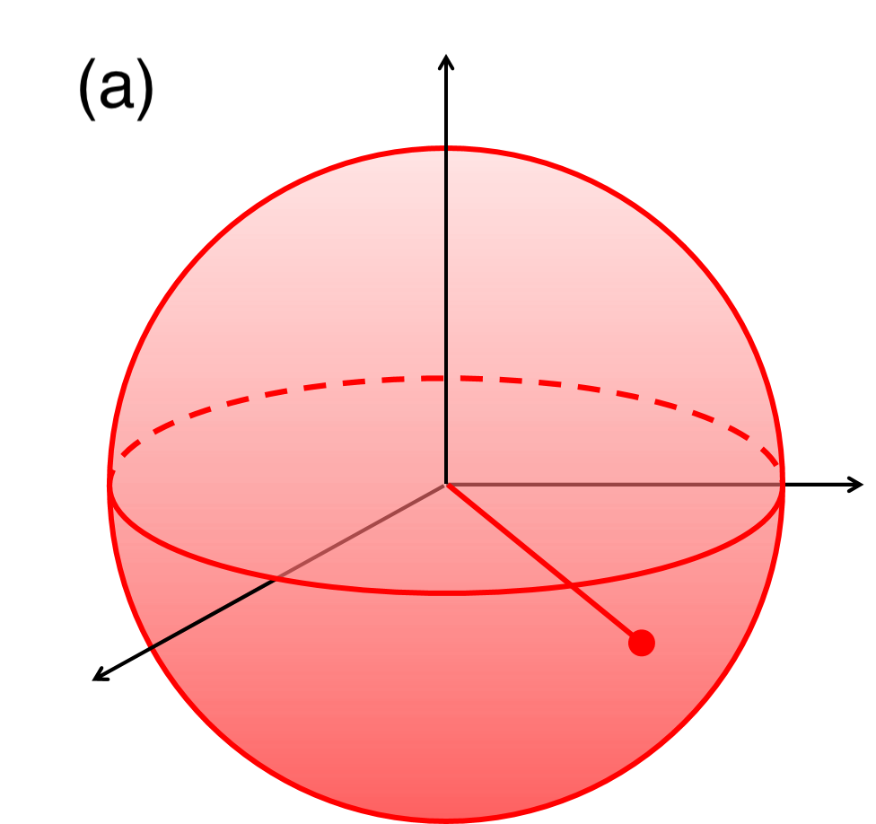
Figure 1: The $N$ dimensional sphere. (a) A high temperature (extended) situation with no metastable states, both in the $p=2$ and $p=3$ models. (b) In the $p=2$, the axes are the eigenvectors $\vec{v}_{1},\dots\vec{v}_{N}$ of the interaction matrix ${\mathbb{J}}$. Only $\vec{v}_{N}$ the eigenvector with largest eigenvalue (and its reversed) are equilibrium states and are highlighted in green. There are no metastable states. (c) In the $p\geq 3$ case there are orthogonal metastable states, some of them shown in the sketch.

The equilibrium properties can be expressed in terms of sums over the states, counted with their multiplicity [59]. This formulation ends up with ${\mathcal{Z}}=\int df\,e^{-N(\beta f-\sigma(\beta,f))}$ where $\sigma=\Sigma/N$ is the complexity per degree of freedom at fixed randomness. The integral runs over free-energy densities and in the large $N$ limit it is dominated by the $f$ that minimizes the expression in the exponential, which could be the minimum $f$ if $\sigma=0$ or the non-trivial solution to $\beta=\partial\sigma/\partial f$ otherwise. The latter case arises in the temperature interval $[T_{s},T_{d}]$. A pinning field method that allows one to select and study metastable states (which are not the equilibrium ones) with this formalism was developed in [49].

The equilibrium properties of the spherical $p\geq 3$ model at $T<T_{s}$ are also derived with a replica analysis with a one step replica symmetry breaking (1RSB) Ansatz in which the elements of the Parisi matrix take two values, organized in square blocks. They represent the overlap between configurations in the same state, $q_{1}=q_{\rm EA}$, and the overlap between configurations in different states, $q_{0}=0$ [19]. The size of the blocks is determined by a parameter which is extremized. Instead, the properties at the threshold are obtained by fixing this parameter requiring marginal stability of the 1RSB Ansatz. Very recently, the static features of the spherical $p$-body model were re-derived with the cavity method [60].

Another way to access the non-trivial metastable states in the landscape is to define an effective potential for the overlap $q=N^{-1}\sum_{i}x^{(1)}_{i}x^{(2)}_{i}$ where $x^{(1)}_{i}$ and $x^{(2)}_{i}$ are two coupled copies of the system (same quenched randomness different configurations). The logarithm of the probability distribution of $q$ defines the so-called Franz-Parisi potential [61], [] Franz-Parisi potential The free-energy of an equilibrium system constrained to have a fixed overlap with a reference equilibrium configuration. which at high temperatures has a single minimum at $q=0$, indicating that the stable phase is completely disordered, while as temperature is lowered, loses convexity, and eventually develops a second minimum at $q\neq 0$ below $T_{d}$, indicating the presence and thermodynamic importance of metastable states.

In the variant with bi-valued variables $x_{i}=\pm 1$, there is another transition at $T_{G}<T_{s}$, where _G stands for Gardner [62]. The free-energy landscape takes on a hierarchical structure and FRSB arises in the replica analysis below $T_{G}$. This transition separates a stable glass phase from a marginally stable one. A sketch is shown in Fig. 2(c). This phenomenon also appears in particle based glassy models in infinite dimensions [63] and in some of the ecological models [64] that we will discuss in Sec. 7.2.

4.4 The mixed $p$ case

We called pure $p$ model the one with a single monomial potential energy, Equation 5. A logical extension is to consider the sum of two such terms with different $p$, say $p$ and $s$. There are several reasons for being interested in these generalizations. In the glassy context, they appear in the mode-coupling approach to super-cooled liquids. In mappings between optimization problems and disordered spin systems, models with “polynomial” energies naturally arise [65]. These mixed models turn out to be much more complex than the pure ones, presumably because they lose the homogeneity of the Hamiltonian. [] Temperature chaos The TAP free-energy stationary points cross, merge or divide as temperature is varied.

Mixed models exhibit temperature chaos [66], that is, the finite temperature metastable states are not simple continuations of the zero temperature ones. Visualized as free-energy levels, there are level crossings [67, 68, 69, 70]. Moreover, the free-energy landscapes at fixed temperature are not layered as the ones of the monomial models. As the free-energy landscapes are so involved, let us only describe them at zero temperature. First of all, they are different for the $(p=2)+s$ and $(p=3)+s$ models, and also diversify when $s$ is modified. In a few words, for the perturbed $p=2$ model the zero-$T$ replica solution goes from RS ($s=0$) to 1RSB ($s=3$ and not too strong perturbation), followed by a combined 1RSB and FRSB structure, with the former/latter for large/small values of the overlap ($s>3$). At sufficiently strong perturbation it is just FRSB. A similar (though different) complex phase diagram arises in the perturbed $p=3$ model [71]. Above the ground states, these models present an exponential number of local minima. In the $p=3,s=4$ model there is an exponential number of marginally stable states in a finite range of energies [72, 73] and not just a single value as in the pure model. All these novel features complicate considerably the dynamics, which is not completely understood yet, see Sec. 5.1.3.

5 RELAXATIONAL DYNAMICS

In this Section we focus on conservative forces $f_{i}=-\partial V/\partial x_{i}$, no external drive, and finite coupling to the bath ($\eta\neq 0$). Typical initial conditions of equilibrium at high temperature $T_{0}\gg T_{d}$ are very energetic and progressively transfer their excess energy to the bath when quenched to $T<T_{0}$. This process can be rapid and let the system equilibrate quickly with the environment, or very slow with peculiar time-dependencies. Initial conditions which know about the free-energy landscape behave differently as we specify below.

In applications of these methods to the glass problem $\gamma/m\gg 1$ and inertia is negligible. The velocities rapidly equilibrate with the environment and reach a Maxwell distribution. One then adopts an over-damped description from the start.

5.1 Slow relaxation and aging

We focus on instantaneous temperature quenches to temperature $T$. Other protocols, like thermal annealing, may be closer to the schemes used in industry and the like but we do not find it necessary to discuss them here. In correspondence with the free-energy landscape properties, the long-time relaxation of the $N\to\infty$ spherical pure $p$ models and their mixed extensions have very different properties depending on $T_{0}$ and how $T$ compares to various characteristic temperatures.

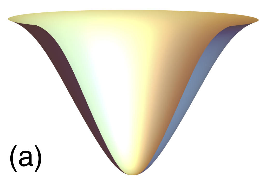
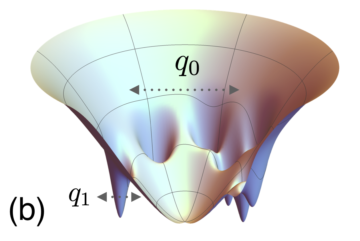
Figure 2: Sketches of the free-energy density landscape close to equilibrium. (a) A single minimum, typical of high temperatures where all effects of the interactions are washed out by the strong thermal fluctuations. (b) Multiple minima of the $p\geq 3$ model at temperatures below $T_{s}$. The parameters $q_{0}$ and $q_{1}=q_{\rm EA}$ indicate the overlap between configurations of different equilibrium states and configurations within the same one, respectively. (c) The hierarchical organization of equilibrium states with relatively low barriers between them as realized in the Sherrington-Kirkpatrick model and Gardner phases. Higher lying metastable states and flat regions as the threshold of the $p\geq 3$ model are not represented in these sketches but can be found in Fig. 5.

5.1.1 The spherical pure $p=2$ case

Quenches at the transition temperature $T=T_{s}$ show critical dynamics. In sub-critical quenches, $T<T_{s}$, from the high temperature phase, $T_{0}>T_{s}$, and no applied ordering field, $\vec{h}=\vec{0}$, the initial conditions tend to align in the course of evolution with $\vec{v}_{N}$ (or its reversed): $\langle\vec{x}\cdot\vec{v}_{N}\rangle\sim t^{3/4}$. This parallels the growth of the zero wave-vector mode, homogeneous order, of finite dimensional coarsening [74].

[] Coarsening or domain growth The progressive growth of order in the symmetry-broken phase across a second order phase transition.

The non-equilibrium character below $T_{s}$ is due to the fact that the system does not reach the required $N^{1/2}$ overlap with ${\vec{v}}_{N}$ in finite time with respect to $N$. This means that it does not achieve spontaneous symmetry breaking in such time scales. Having said so, the energy density gets close to its equilibrium value, $e(t)\sim e_{\rm eq}+ct^{-\alpha}$, with $e_{\rm eq}$ a function of $T/J$, $c$ a numerical constant and $\alpha=1$. In a coarsening problem, this decay estimates the growing “length” since the excess energy is localized on regular interfaces between domains.

The two-time correlation evolves in two two-time scales. A rapid and stationary one

$$\lim_{t_{2}\to\infty}C(t_{1},t_{2})=C_{\rm st}(t_{1}-t_{2})\quad\mbox{with}\quad C_{\rm st}(0)=1-q\;\;\mbox{and}\lim_{t_{1}-t_{2}\to\infty}\!\!C_{\rm st}(t_{1}-t_{2})=0\;,$$ (20)

and a slow and aging one [] AgingOlder systems relax more slowly than younger ones.

$$\lim_{t_{1},t_{2}\to\infty}\!\!C(t_{1},t_{2})=C_{\rm ag}\left(\frac{t_{1}}{t_{2}}\right)\;\;\mbox{with}\lim_{t_{1}\to t^{+}_{2}\to\infty}\!\!C_{\rm ag}\left(\frac{t_{1}}{t_{2}}\right)=q\;\;\mbox{and}\lim_{t_{1}\gg t_{2}}\!\!C_{\rm ag}\left(\frac{t_{1}}{t_{2}}\right)=0\;.$$ (21)

The high-temperature initial conditions are completely forgotten asymptotically, in the sense that $C(t,0)\to 0$. A sketch of this decay appears in Fig. 3(a), with the different curves corresponding to different $t_{2}$, increasing from left to right.

The time $t_{2}$ is the age of the system, the time spent at the working conditions before starting the measurement. In the long $t_{2}$ limit, a sharp separation in the decay of $C$ is achieved at $C=q>0$. This is the definition of the order parameter given by Edwards and Anderson in their seminal paper on spin-glasses [18]. In this model, it coincides with the global equilibrium order parameter $q=q_{\rm EA}=N^{-1}\sum_{i=1}^{N}[\langle x_{i}\rangle^{2}]$ at the working temperature. One can then propose the notion of correlation scale, there being two of them in this problem, $q\leq C<1$ and $0\leq C<q$. Correlation scaleRange of correlation values with distinct properties from the rest.

The complete functional form $C_{\rm ag}(t_{1}/t_{2})$ is known exactly. In analogy with coarsening, it is interpreted as evidence for an algebraic growth [2] of the typical linear length of the domains $R(t)\sim t^{1/z}$, with a dynamic exponent $z$ which cannot be fixed in this case, since a change in $z$ would simply change the scaling function. Still, one can claim $C_{\rm ag}(R(t_{1})/R(t_{2}))$ where times appear only through $R$, the proxy for the typical length evaluated at the two times. The essence of dynamic scaling is that all $n$-time correlations should be functions of $R(t_{1})/R(t_{2}),\dots,R(t_{n-1})/R(t_{n})$, a property which also holds in this model.

A similar separation applies to the integrated linear response function:

$$\chi(t_{1},t_{2})\equiv\int_{t_{2}}^{t_{1}}dt^{\prime}\,R(t_{1},t^{\prime})\;\;\;\;\mbox{with}\;\;\;\;\chi(t_{1},t_{2})\to\chi_{\rm st}(t_{1}-t_{2})+\chi_{\rm ag}(t_{1},t_{2})$$ (22)

together with $\chi_{\rm st}(0)=0$,

$$\lim_{t_{1}-t_{2}\to\infty}\chi_{\rm st}(t_{1}-t_{2})=\frac{1}{T}(1-q)\;\;\;\;\;\mbox{and}\;\;\;\;\chi_{\rm ag}(t_{1},t_{2})=t_{2}^{-1/2}f_{R}\left(\frac{t_{1}}{t_{2}}\right)\xrightarrow[t_{2}\to\infty]{}0\;.$$ (23)

In the rapid regime the correlation and linear response satisfy FDT with the temperature of the bath. Instead, FDT is modified in the slow scale in a maximal way, as the integrated linear response vanishes asymptotically.

In sub-critical quenches the separation of time-scales is additive as stationary and aging parts add up to yield the total two-time functions. A quench to the critical temperature would yield instead a multiplicative separation, $C=C_{\rm st}C_{\rm ag}$ and $\chi=\chi_{\rm st}\chi_{\rm ag}$, concomitant with the fact that $q=0$ at criticality. The relations between linear response and correlation functions in critical quenches have been studied in great detail [75].

An ordering field $h>0$ changes this picture: it introduces a finite time-scale $t_{\rm eq}=[(2+h^{2})/\sqrt{1+h^{2}}-2]^{-1}\sim h^{-4}$ for $h\sim 0$, after which the dynamics become stationary and equilibrium is reached even at low temperatures [76].

The properties exposed above are shared in full qualitative, and sometimes even quantitative, form by finite dimensional models of domain growth and phase separation, such as the two or three dimensional Ising model with different kinds of stochastic microscopic updates. Examples and further details can be found in Refs. [3, 4, 5].

5.1.2 The spherical pure $p\geq 3$ case

In this model there are three characteristic temperatures: the static critical temperature $T_{s}$, the dynamic critical temperature $T_{d}$, and $T^{*}$ the maximal temperature at which metastable minima of the free-energy density exist.

5.1.2.1 High temperature instantaneous quenches

At $T>T_{d}$, initial conditions prepared in equilibrium at $T_{0}>T_{d}$ relax to the single equilibrium state. After a short transient, $t_{2}$ $\stackrel{{\scriptstyle>}}{{\sim}}$ $t_{\rm st}$, the dynamics become stationary, $C(t_{1}-t_{2})$ and $R(t_{1}-t_{2})$. At very high temperatures $T\gg T_{d}$ these functions quickly decay exponentially. Close to but still above $T_{d}$ the dynamics dramatically slow down. For all $T>T_{d}$, the energy density approaches the equilibrium value $e(t)\to e_{\rm eq}$ asymptotically. $T_{d}$ is the dynamical critical temperature below which all this no longer happens.

Close to $T_{d}$ a two-step relaxation develops: a first rapid decay from $C(0)=1$ towards a plateau at $q_{d}$, a slow evolution around it and, eventually, a further very slow decay towards zero. The plateau length is longer and longer as $T$ gets closer to $T_{d}$, representing the fact that the system keeps an increasingly long memory of the initial configuration, which it will eventually forget. These features are typical of super-cooled liquids. [] Super-cooled liquids A liquid cooled beyond the crystallization point. The evolution around $q_{d}$ is the $\beta$-relaxation and it is algebraic with two exponents, $C(t_{1}-t_{2})\sim q_{d}+c(t_{1}-t_{2})^{-a}$ and $C(t_{1}-t_{2})\sim q_{d}-\overline{c}(t_{1}-t_{2})^{b}$, related by $\Gamma^{2}(1+b)/\Gamma(1+2b)=\Gamma^{2}(1-a)/\Gamma(1-2a)=(T/2)\,\overline{V}^{\prime\prime\prime}(q)/(\overline{V}^{\prime\prime}(q))^{3/2}$. The structural or $\alpha$-relaxation below the plateau, $C(t_{1}-t_{2})=f((t_{1}-t_{2})/\tau_{\alpha})$, can be characterized in terms of a structural relaxation time which diverges as $\tau_{\alpha}\sim|T-T_{d}|^{-\gamma}$ with $\gamma$ a “critical” exponent satisfying $\gamma=1/(2a)+1/(2b)$. At infinite time separation the decorrelation is complete, $f(\infty)=0$. The sketch in Fig. 3(a) represents this case, with the curves at different temperatures decreasing from left to right.

In terms of trajectories on the spherical configurational space, the interpretation is the following. Let us assume that $t_{1}\geq t_{2}\gg t_{0}$. At $t_{1}$ such that $t_{1}-t_{2}$ is short, the position vector $\vec{x}(t_{1})$ remains close to the reference one at $t_{2}$, $\vec{x}(t_{2})$, and $C(t_{1}-t_{2})>q_{d}$. Instead, at longer $t_{1}-t_{2}$, $\vec{x}(t_{1})$ drifts towards other equilibrium configurations, $C(t_{1}-t_{2})<q_{d}$, and eventually decorrelates completely from the reference one, $C(t_{1}-t_{2})\to 0$.

The integrated linear response $\chi$ also develops an additive separation of scales, depicted in Fig. 3(b). The correlation plateau at $q_{d}$ translates into a plateau at $(1-q_{d})/T$ in $\chi$. Correlation and linear response are related by the FDT: $T\,R(t_{1}-t_{2})=-d_{t_{1}}C(t_{1}-t_{2})$, for $t_{1}-t_{2}\geq 0$, for all $t_{1}-t_{2}$.

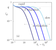
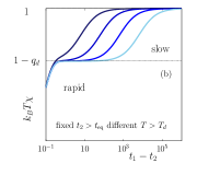
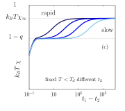
Figure 3: (a) The two-time correlation $C(t_{1},t_{2})$. The sketch can represent different cases. First, the equilibrium decay at different temperatures $T$ getting closer to $T_{d}$ from above and from left to right in the $p\geq 3$ model. The two-step relaxation is separated by a plateau at $q=q_{d}$. Second, the out of equilibrium decay below $T_{d}$ in the $p\geq 3$ model, or below $T_{d}=T_{s}$ in the $p=2$ one, with the different curves calculated for increasing waiting times $t_{2}$ from left to right. (b) The integrated linear response times working temperature, $k_{B}T\,\chi(t_{1},t_{2})$ in the equilibrium $p\geq 3$ model at different temperatures close to $T_{d}$, decreasing from left to right (we restored $k_{B}$). (c) The integrated linear response $\chi(t_{1},t_{2})$ out of equilibrium at a single temperature $T<T_{d}$ and for different $t_{2}$ increasing from left to right.

5.1.2.2 Low temperature instantaneous quenches

Below $T_{d}$, initial conditions prepared in equilibrium at $T_{0}>T_{d}$ reduce their energy until reaching the threshold energy which is macroscopically higher than the equilibrium one, $e(t)\to e_{\rm th}+ct^{-\alpha}$ with $e_{\rm th}>e_{\rm eq}$. The relaxation takes place in two two-time scales, say, $(t_{1}-t_{2})/\tau_{\alpha}(t_{2})<1$ and $(t_{1}-t_{2})/\tau_{\alpha}(t_{2})>1$. In the first one, $C$ and $R$ behave as if the system were equilibrated with the environment, they are stationary and satisfy FDT. In the second one, they are non-stationary with aging, that is, older systems decay more slowly than younger ones. This represents the fact that the system keeps exploring phase space with a velocity that diminishes with the elapsed time after the quench. The physical aging of glasses has been studied experimentally during the last century since the implications on the material properties have industrial relevance. A recent non-technical discussion can be found in Ref. [77]. In the slow regime, the FDT applies but with a different temperature from the one of the bath [31]; this is related to the fact that the threshold energy level is asymptotically sampled uniformly, hence attaining a sort of effective equilibrium at an effective temperature [78]. For $T_{0}>T_{d}$, $T_{\rm eff}>T$, recalling the fact that the system has been quenched from high temperature and the long time-delay dependencies (low frequencies) have not had enough time to equilibrate with the bath. The operationally defined $T_{\rm eff}$ then meets the phenomenological idea of fictive temperatures commonly used in the glass literature [79]. [] Effective temperatures The slow dynamics self-organizes to take place at a temperature that is different from the one of the bath, and has a thermodynamic meaning. [] Weak ergodicity breaking The approach to the plateau suggests ergodicity breaking; however, there is no full arrest and $C\to 0$ asymptotically.

The separation between scales is sharp in the infinite waiting-time limit:

$$\lim_{t_{2}\to\infty}C(t_{1},t_{2})=C_{\rm st}(t_{1}-t_{2})\qquad\qquad\quad\mbox{with}\qquad\lim_{t_{1}-t_{2}\to\infty}C_{\rm st}(t_{1},t_{2})=0\;,$$ (24)

$$\lim_{t_{1},t_{2}\to\infty}C(t_{1},t_{2})=C_{\rm ag}({\rm h}(t_{1})/{\rm h}(t_{2}))\qquad\mbox{with}\qquad\lim_{t_{1}\to t^{+}_{2}\to\infty}C_{\rm ag}(t_{1},t_{2})=q\;,$$ (25)

together with $C_{\rm st}(0)=1-q$ and $\lim_{t_{1}\gg t_{2}}C_{\rm ag}({\rm h}(t_{1})/{\rm h}(t_{2}))=0$. These properties have been named weak ergodicity breaking [80, 31]. The numerical solution of the Schwinger-Dyson equations suggests that ${\rm h}(t)\propto t$ [81, 72]. The $\beta$ relaxation around the plateau is also controlled by two exponents, $C(t_{1}-t_{2})\sim q_{d}+c(t_{1}-t_{2})^{-a}$ and $C(t_{1},t_{2})\sim q_{d}-\overline{c}({\rm h}(t_{1})/{\rm h}(t_{2}))^{b}$, related by $(T/T_{\rm eff})\,\Gamma^{2}(1+b)/\Gamma(1+2b)=\Gamma^{2}(1-a)/\Gamma(1-2a)=(T/2)\,\overline{V}^{\prime\prime\prime}(q)/(\overline{V}^{\prime\prime}(q))^{3/2}$ [82].

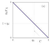
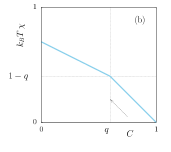
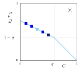
Figure 4: The parametric construction $\chi(C)$. Both axes are parametrized by $t_{1}-t_{2}$ which runs from 0 ($C=1,\chi=0$) to $\infty$ ($C=0,\chi=\chi_{\infty}$). (a) In any equilibrium situation. If close but above $T_{d}$ in models with a RFOT, $q_{d}$ indicates the value of $C$ on the plateau. (b) Out of equilibrium below $T_{d}$ in the $p\geq 3$ model. The dotted arrows in (a) and (b) indicate the sense in which $t_{1}-t_{2}$ increases. (c) Thermal noise induced fluctuations on case (b). The data points are obtained at fixed $t_{1}$ and $t_{2}$. The skyblue point represents the values averaged over thermal noise while the four dark blue points would be the results of retarded or advanced runs with respect to the average, constrained to lie on the $\chi(C)$ curve following time-reparametrization $t\mapsto{\rm h}(t)$.

While the linear response vanishes at long-time delays,

$$\lim_{t_{1}\gg t_{2}}R(t_{1},t_{2})=0\;,$$ (26)

the integrated linear response $\chi(t_{1},t_{2})=\int_{t_{2}}^{t_{1}}dt\,R(t_{1},t)$ does not, an effect called weak long-term memory [31]. A sketch with the integrated linear response for increasing $t_{2}$ from left to right is displayed in Fig. 3(c). Moreover,

$$\lim_{\begin{subarray}{c}t_{2}\to\infty\\ C(t_{1},t_{2})=C\end{subarray}}\chi(t_{1},t_{2})=\chi(C)=\left\{\begin{array}[]{ll}T^{-1}\,(1-C)&q\leq C\leq 1\\ T^{-1}\,(1-q)+T_{\rm eff}^{-1}\,(q-C)&0\leq C<q\end{array}\right.$$ (29)

similarly to Equation 23, and $T_{\rm eff}>T$. [] Weak long-term memoryThe linear response integrated over a diverging period is finite but the instantaneous one vanishes at long time delays.

This piece-wise relation is a particular case of the more general parametric one

$$\lim_{\begin{subarray}{c}t_{2}\to\infty\\ C(t_{1},t_{2})=C\end{subarray}}\chi(t_{1},t_{2})=\chi(C)\qquad\mbox{with}\qquad\frac{1}{T_{\rm eff}(C)}=\chi^{\prime}(C)\;.$$ (30)

In terms of evolution in the free-energy landscape, the highly energetic initial configurations approach the threshold level and keep straying along it without penetrating below it in finite times with respect to system size. The threshold is the basin of attraction of all high temperature initial conditions [72]. The decay of the correlation in two two-time scales indicates that the threshold is made of almost flat “channels” which trap the system in “transverse” directions but let it drift in “longitudinal” ones. Thus, the correlation first decays from $C(t_{1},t_{1})$ to a maximal decorrelation $q=q_{\rm th}$, the transverse size of the channels, for $t_{1}-t_{2}\to\infty$. The value $q_{\rm th}$ coincides with $q_{\rm th}=N^{-1}\sum_{i}[\langle x_{i}\rangle^{2}]$ where $\langle x_{i}\rangle$ are the local order parameters of the threshold free-energy level. Then, $C$ further decreases from $q_{\rm th}$ to zero in an aging manner, since getting closer and closer to completely flat directions [31, 83].

(a)                                             (b)               (c)               (d)

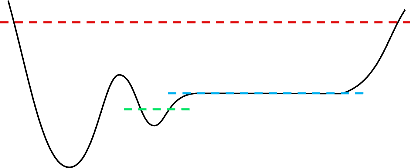
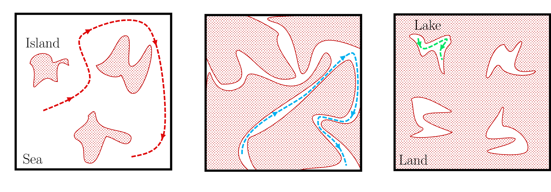
Figure 5: A sketch of the dynamics trajectories in the free-energy density landscape of the $p\geq 3$ spherical model. $(a)$ A “transverse” cut, with a level above threshold (dashed red), at threshold (dashed blue and below threshold (dashed green). The free-energy density is defined on an $N$ dimensional space and $N-1$ coordinates are therefore hidden in this sketch. The threshold is mostly flat while the sub-threshold states are mostly stable. Three top views of the landscape taken at different free-energy levels: above $(b)$, at $(c)$ and below $(d)$ the threshold. The “islands” represent barriers protruding above the selected level. The “sea” represents the available space for the system to move or relax. The threshold is visualized as being very ramified and expanding along phase space.

The dynamics close and below $T_{d}$ have the qualitative features of the (schematic) Mode Coupling Theory (MCT) description of the slowing down of fragile glasses [29, 6, 84]. There is a technical reason for this. The introduction of quenched randomness exactly renders all diagrams from the field-theoretic solution sub-leading except for the melonic ones [29]. The idea of “simplifying” the underlying model by introducing randomness, follows the same logical path taken by Kraichnan in the formulation of the direct interaction approximation for the Navier-Stokes equation [85]. [] Mode Coupling TheoryApproximate self-consistent equations ruling the evolution of selected dynamical correlations in interacting particle models, e.g. the intermediate scattering function.

5.1.2.3 Instantaneous quenches within metastable states

The evolution, below their spinodal, of initial conditions prepared in one of the metastable states remains confined within this same state [61, 32]. This confirms the fact that the barriers surrounding these states diverge with $N$ and cannot be surmounted in times that do not scale conveniently with $N$. After a short transient the dynamics become stationary. The overlap of the time-dependent configuration with the initial one saturates to a non-zero value, $C(t_{1}-0)\to\overline{q}_{1}$. Accordingly, also $\lim_{t_{1}\gg t_{2}\gg t_{0}}C(t_{1}-t_{2})\to q_{1}>0$. These two overlaps characterize the similarity of the initial state with the final one, $\overline{q}_{1}$, and the size of the final state, $q_{1}$. The FDT holds, reflecting the fact that the system achieves a restricted equilibration within the chosen metastable state, in the manner of conventional ergodicity breaking. [] Strong ergodicity breakingThe decorrelation is not complete.

5.1.2.4 A pictorial view

Figure 5 depicts graphically the different situations discussed above in more abstract terms. The panels (b)-(d) represent a top view of the free-energy landscape and how it can be explored in quenches from $T_{0}>T_{d}$ to $T>T_{d}$ (b), $T_{0}>T_{d}$ to $T<T_{d}$ (c), and the dynamics within confining metastable states $T_{0}<T_{d}$ (d).

5.1.3 The spherical mixed $p$ case

The relaxation of the spherical mixed $p-s$ models is more complex and still the subject of active research.

The analysis of the state following dynamics in the $p=3$, $s=4$ case, for $T_{s}<T$ $<T_{0}<T_{d}$, was carried out in [67, 68, 86, 87, 88]. Above a special working temperature the relaxation is as in the pure model, in the sense that the system equilibrates within the transformed original state and $C(t,0)$ approaches a non-zero value consistent with metastable (time-independent) calculations. Below it, these solutions no longer exist. Instead, the dynamics ages forever with the very unusual feature of keeping memory of the initial condition, via a non-zero asymptotic $C(t,0)$, and thus realizing strong ergodicity breaking combined with aging. Below this special temperature the initial state opens up into a marginal region of the free-energy landscape, which lies below the level approached with quenches from $T_{0}\to\infty$. The configurations in these new marginal states do keep, however, a finite similarity with the initial ones.

More recently, these results were complemented by the numerical study of the gradient descent ($T=0$) dynamics of initial conditions thermalized close [72] and far above [89] $T_{d}$, for a wide variety of $s$ terms added to both $p=2$ and $p=3$. By numerical we mean the numerical solution of the Schwinger-Dyson equations. Differently from the monomial case, the asymptotic configurations seem to keep memory of the initial ones, $\lim_{t\to\infty}C(t,0)>0$, for all $T_{0}$ and, presumably, for all $s\neq p$. The dynamics remain confined to a restricted manifold that depends on the initial condition. Moreover, the asymptotic energy is not the threshold one at which dominant minima become saddles (as in the pure case), but a higher value, which depends on $T_{0}$. This level is also a marginally stable region of the potential energy landscape and, consequently, the energy density (and other one-time quantities) converge algebraically to their asymptotic values. Therefore, in these models there is no unique basin of attraction for all high-temperature initial conditions. Concerning the scaling of $C$ and $\chi$, the data suggest that they are both functions of $t_{1}/t_{2}$. $\chi(C)$ takes a non-trivial functional form, thus invalidating the identification of simple aging with a single $T_{\rm eff}$ value.

The features explained above were obtained numerically and are limited in precision and time span, so changes in the truly asymptotic regime cannot be excluded. Unfortunately, no analytic solution, compatible with the numerical results, has been derived yet for the mixed case. While a connection between dynamic and metastable behaviour derived from replica calculations was clear in monomial models, this is still lacking for the $p+s$ cases.

5.1.4 Models in the Sherrington-Kirkpatrick class

The Sherrington-Kirkpatrick model, as already stated, belongs to a different equilibrium class (FRSB, hierarchical organization of equilibrium states with all possible overlaps between them) and this has a dynamic correspondence. The out of equilibrium Langevin relaxation of soft continuous spins [90, 30], after a quench from $T>T_{s}$, occurs in an infinite sequence of times-scales [91, 92]. The FD relation is linear $T\chi(C)=1-C$ for $C>q$ and takes a non-trivial form for $C<q$.

In its original strictly Ising version other algorithms can be developed to search for the configuration that corresponds to the optimum energy, see [93, 94] for recent progress.

5.2 Effective temperatures and multi-thermalization

The relaxation of the monomial model takes place in two scales, each with its own temperature: the fast one is the one of the external bath while the slow scale arranges to have its own value self-consistently selected by the initial condition and the internal interactions. There are other models (e.g. the Sherrington-Kirkpatick or the $p$-spin in the Gardner phase, both with soft variables) for which the relaxation follows a sequences of scales, each with its own temperature [91, 92, 64]. All these cases are included in $-1/T_{\rm eff}(C)=\chi^{\prime}(C)$, in the long $t_{2}$ limit. This definition has a thermodynamic meaning explained in [78, 95] and later extensively investigated [96]. $T_{\rm eff}$ can be accessed with thermometers which tune their measurement to the desired correlation scale. The degrees of freedom evolving in the same scale are equilibrated among them and share the same value of $T_{\rm eff}$. Instead, the ones which evolve in different scales are not and can have different temperatures. This same scenario can be induced on, e.g., a harmonic oscillator by coupling the particle’s position to a multi-bath with different temperatures and time-scales [95, 97] (different pairs $\Gamma_{R}$ and $\Gamma_{C}$ related by FDTs at different temperatures). In the case in which the baths evolve in widely separated time-scales their effects can be mimicked by quasi-static random fields [95]. This formalism has been recently exploited [64] to recover the aging with effective temperature scenario from the single effective variable formalism. The effective temperature also has an intuitive meaning. For quenches from disordered/extended initial conditions to low temperature phases $T_{\rm eff}(C<q)\geq T$. For inverse quenches in which an ordered/localized initial configuration is evolved under conditions that render it more disordered, $T_{\rm eff}(C<q)\leq T$. Accordingly, the slow scales, $C<q$, remember the initial conditions and their “more ordered” or “more disordered” nature, compared to the target one at the running temperature. In $p$ body models $T_{\rm eff}$ also finds a fascinating relation with the structure of the free-energy density explored by the dynamics:

$$\frac{1}{T_{\rm eff}(C<q)}=\left.\frac{\partial\sigma(f,T)}{\partial f}\right|_{f_{\rm th}}\!\!\!\!.$$ (31)

with $\sigma$ the complexity per degree of freedom [49]. The effective temperature concept, the connection with phenomenological ideas, and its measurement in a large variety of finite $d$ and systems has been reviewed in Ref. [96]. More recent applications in the context of learning in neural networks will be discussed in Sec. 7.3.

5.3 Time reparametrization invariance

A very general feature of the slow dynamics is that the time-dependence of $C$ and $R$ is sensitive to vanishingly small changes in the equations of motion. Take for example the case of ferromagnetic coarsening. An arbitrary small random field changes the growth of the equilibrated domains from algebraic to logarithmic. In mean-field disordered systems weak non-conservative forces may destroy the aging relaxation and render the evolution stationary (Sec. 7). This extreme sensitivity is the consequence of the slow relaxation taking place along flat regions of the free-energy landscape. These facts have a mathematical counterpart in the invariances of the Schwinger-Dyson equations.

In the absence of an external force $\vec{h}=\vec{0}$, the low temperature evolution of the $p\geq 3$ models acquires a (global) time-reparametrization invariance [30, 31, 90, 98, 99]:

$$t\mapsto{\rm h}(t)\;,\;\quad\;C(t_{1},t_{2})\mapsto C({\rm h}(t_{1}),{\rm h}(t_{2}))\;,\;\quad\;R(t_{1},t_{2})\mapsto\frac{d{\rm h}(t_{2})}{dt_{2}}\,C({\rm h}(t_{1}),{\rm h}(t_{2}))\;.$$ (32)

Under these transformations, certain relations between observables and, in particular, the ones between linear response and correlation, remain unmodified. For example, $T\chi(t_{1},t_{2})\;\equiv\;T\,\int_{t_{2}}^{t_{1}}dt\,R(t_{1},t)=1-C(t_{1},t_{2})$ for $t_{1}-t_{2}>0$ is still $T\chi(C)=1-C$ for any way of measuring time, be it as $t$ or any other monotonic ${\rm h}(t)$. This feature extends to any relation between $\chi$ and $C$ of the form $\chi(C)$.

The time-reparametrization invariance implies that, in the asymptotic long times limit, there exists a family of solutions to the Schwinger-Dyson equations linked to each other by one of the transformations in Equation 32. This is a consequence of the fact that the proper measure of “time distance between two times $t_{1}$ and $t_{2}$” is the value of the correlation $C(t_{1},t_{2})$, and not the readout of the “wall clock” in the laboratory [31]. This idea was recently applied to interpret multi-speckle dynamic light-scattering data on an aging molecular glass former [100, 101]. The actual parametrization is determined by the matching between the short time-difference behavior in the fast regime (which acts as a selection operator) and the long time-difference slow one. The analytic treatment of this matching is still open.

Importantly enough, the invariance of the Schwinger-Dyson equation needs a finite $T_{\rm eff}$ in the slow relaxation. In the $p=2$ model, $T_{\rm eff}\to\infty$ and the symmetry is reduced to scale invariance, $t\mapsto at$ [102]. This is another distinction between the two types of models.

It was argued that time reparametrization invariance should be at the origin of dynamic fluctuations in glassy systems [99, 103, 104]. The fluctuations would then be due to dynamic fluctuations in the local time parametrizations ${\rm h}(\vec{r},t)$ in a finite dimensional system [99, 103]. An effective theory for these fluctuations was constructed and numerical and experimental tests were proposed and performed [104]. In the fully-connected models, similar fluctuations in the global observables are triggered by thermal noise in finite size systems. A sketch of how they would appear in a $\tilde{\chi}(\tilde{C})$ relation, with $\tilde{\chi}$ and $\tilde{C}$ not averaged over noise is displayed in Fig. 4(c).

Such invariances have recently played a crucial role in the interpretation of the Sachdev-Ye-Kitaev (SYK) model [105] as a toy model of holography [106, 107], see Sec. 8.

5.4 Higher order correlations and length-scales

The correlation $C(t_{1},t_{2})$ is playing the rôle of the order parameter of the dynamic transition in the RFOT scenario as realized, e.g., by the spherical $p\geq 3$ models. Although there is no proper length-scale in this model, by analogy, the divergence of its fluctuations [108, 109, 110, 111],

$$G_{4}(t_{1},t_{2})=N^{-1}[\langle(\sum_{i}x_{i}(t_{1})x_{i}(t_{2}))^{2}\;\rangle-\langle\sum_{i}x_{i}(t_{1})x_{i}(t_{2})\rangle^{2}\;]\;,$$ (33)

has been used as an indication that a dynamic length scale diverges as the glassy arrest is approached from above. For vanishing $\epsilon=(T-T_{d})/T_{d}$, the distance from the critical point, and in the long time delay limit, $G_{4}$ becomes stationary and scales as

$$G_{4}(t_{1}-t_{2})=\left\{\begin{array}[]{ll}\dfrac{1}{\sqrt{\epsilon}}\;f_{\beta}\left((t_{1}-t_{2})\epsilon^{1/(2a)}\right)&\qquad t_{1}-t_{2}\sim\tau_{\beta}\sim\epsilon^{-1/(2a)}\;,\\[12.0pt] \dfrac{1}{\epsilon}\;f_{\alpha}\left((t_{1}-t_{2})\epsilon^{\gamma}\right)&\qquad t_{1}-t_{2}\sim\tau_{\alpha}\;,\end{array}\right.$$ (36)

in the $\beta$ and $\alpha$ regimes, respectively. The scaling functions satisfy $f_{\beta}(x)\propto x^{a}$ for $x\ll 1$ and $f_{\beta}(x)\propto x^{b}$ for $x\gg 1$, while $f_{\alpha}(x)\propto x^{b}$ when $x\ll 1$ and vanishes at large $x$. Therefore, it progressively diverges upon $T$ getting closer to $T_{d}$ from above. At fixed temperature below $T_{d}$, the role played by the distance from criticality $\epsilon$ is now the one of the waiting time. The scaling forms in Equation 36 have to be modified accordingly [112].

Experimentally, susceptibilities are easier to access than correlations. Connections between $G_{4}$ and non-linear susceptibility via generalizations of the FDT, much in the same way as the ordinary correlation function is linked to the linear susceptibility, have been established [111, 113, 114]. This idea has been investigated, see [115] for an extensive account. Attempts to go beyond this description, close to $T_{d}$ and in the $\beta$ relaxation regime, and write an effective theory of fluctuations were carried out in [116, 117], see also [118].

5.5 Large dimensionality

The equations discussed so far make no reference to real space; they hold for systems with all-to-all interactions. However, in physical systems interactions have a finite range, and one should include this ingredient in their description.

In strongly interacting cases, large dimensional expansions are a possible line of attack. The Langevin equation for an effective degree of freedom moving in an effective potential was derived in Refs. [119, 120], in the spirit of the single variable Equation 17. The key difference is that in the large $d$ treatment the memory kernel and effective noise correlation have to be determined by a self-consistent implicit functional of $C$ and $R$, while in Equation 15 – corresponding to the schematic MCT – they were simple functions of them.

The $d\to\infty$ equations under equilibrium conditions were successfully analyzed both analytically and numerically. The ensuing qualitative features are the ones of the spherical $p$ models but the details are different (like the values of the exponents $a$ and $b$). Numerous facts of equilibrium hard sphere super-cooled liquids were derived with this formalism, and numerical simulations confirmed the dimensional robustness of some of the predictions. In particular, the critical properties of the jamming transition at infinite pressure were very successfully described by treating them as mechanically marginally stable packings [121]. The out of equilibrium (aging) case has, for the moment, defied numerical integration and is not under control yet [122, 123]. A recent review [121] and a book [124] summarized the technical aspects and outcome of the $d\to\infty$ method.

The dynamical transition in the $d\to\infty$ limit should be quite fragile and disappear in finite dimension. Activated processes should overcome the finite barriers between metastable states. The $d\to\infty$ approach could open the door to a systematic investigation of $1/d$ corrections.

5.6 Finite number of degrees of freedom

The simplest playground to gain insight on how to characterize these activated processes in a large dimensionality space is to study the same models with large but finite number of degrees of freedom. Since activated processes should take an exponentially long time, $t\sim e^{AN}$, to complete, using finite and not too large $N$ may render them accessible numerically.

Models with two-body interactions are especially simple in this respect. The crossover between the dynamics as in the $N\to\infty$ limit and the ones that feel the finite $N$ is controlled by the distribution of eigenvalues of ${\mathbb{J}}$ close to its edge [125, 126]. The low temperature relaxation from random initial conditions takes place in three regimes. The algebraic time-dependencies in the first one are essentially the ones of $N\to\infty$ Next comes a faster algebraic regime determined by the distribution of the gap between the two extreme eigenvalues of ${\mathbb{J}}$, $\lambda_{N}-\lambda_{N-1}$. Finally, an exponential regime takes over and it is determined by the minimal gap sampled in the disorder average. Concerning initial states which are almost projected on the saddles of the potential energy landscape, with deviations ${\mathcal{O}}(N^{-\nu})$ from perfect alignment, the system escapes the initial configuration in a time-scale scaling as $\ln N$ after which the dynamics no longer “self-averages” with respect to the initial conditions.

In the more interesting $p\geq 3$ cases, this analysis was mostly done with Monte Carlo simulations of the bi-valued (Ising) version [127, 128, 129, 130, 131, 132, 133]. In particular, the statistics of trapping times in the metastable states, trap energies, and energy barriers were considered in [131, 132, 134, 133]. One of the aims of these works was to infer, from these measurements which would be the best trap model [80, 135, 136, 137] description of the data. The program is not finished and more refined simulations and analysis are needed to reach a faithful conclusion.

5.7 Mathematical formalization

The literature on the formalization of the theoretical physicists derivations and results is continuously growing. Some examples are the rigorous derivation of the Schwinger-Dyson equations [40], the proof that the $p\geq 3$ model ages (on time scales that scale with $N$) [138], and many refined analyses of the free-energy landscapes [139, 140].

6 HAMILTONIAN DYNAMICS

The search for a statistical description of the asymptotic evolution of isolated many-body quantum systems has received much attention in recent years due, in particular, to the practical realization of closed ultra-cold atomic systems [7], and the study of their evolution under various circumstances. The main question posed in this context is: under which conditions a large closed system can act as a bath on itself and let local observables be described with a static average over a canonical Gibbs-Boltzmann density operator? In cases in which this is not possible, the next issue is whether there is a density operator playing this role and if so which one.

These very same questions can be posed in a classical setting, whereby the classical mechanics evolution of an isolated many-body model, starting from selected initial conditions, is examined. Whenever ergodicity applies, time-averages and statistical averages of non-pathological phase space $(\vec{p},\vec{x})$ dependent macroscopic observables, $A(\vec{p},\vec{x})$, coincide. More precisely, in the $N\to\infty$ limit there is a time $t_{\rm erg}$ after which the time-average [] Ergodicitythe equivalence of time and statistical averages of non-pathological observables.

$$\overline{A(\vec{p},\vec{x})}\equiv\lim_{\tau\to\infty}\frac{1}{\tau}\int_{t}^{t+\tau}\!\!dt^{\prime}\;A(\vec{p}(t^{\prime}),\vec{x}(t^{\prime}))$$ (37)

with $t>t_{\rm erg}$ reaches a constant which can also be calculated with the statistical average

$$\langle A(\vec{p},\vec{x})\rangle\equiv\int d\vec{p}\,d\vec{x}\;\rho(\vec{p},\vec{x})A(\vec{p},\vec{x})$$ (38)

with a suitable $\rho(\vec{p},\vec{x})$. In standard statistical physics the measure $\rho(\vec{p},\vec{x})$ is the microcanonical one, flat over the constant energy surface in phase space, when just the energy of the system is conserved. Alternatively, if one focuses on a selected part of the system, the measure becomes the canonical one, ${\mathcal{Z}}^{-1}\,e^{-\beta{\mathcal{H}}(\vec{p},\vec{x})}$, with an inverse temperature $\beta$ and the Hamiltonian ${\mathcal{H}}$ evaluated in the selected part of phase space. The inverse temperature fixes $\langle{\mathcal{H}}\rangle$ where the average is taken over the measure $\rho$, and controls the energy fluctuations. If the system has a few other constants of motion, $I_{k}(\vec{p},\vec{x})$, the microcanonical measure is still flat over the corresponding reduced sector of phase space, and the canonical one is $\rho(\vec{p},\vec{x})={\mathcal{Z}}^{-1}\,e^{-\sum_{k}\gamma_{k}I_{k}(\vec{p},\vec{x})}$ with $\gamma_{k}$ fixing the average and the fluctuations of $I_{k}$.

In terms of Equations 1, the dynamics we are thinking about here corresponds to $\eta=0$, $\vec{h}=\vec{0}$ and $f_{i}=-\partial V/\partial x_{i}$ with the $p$ body $V$. Different kinds of initial conditions, which we called extended and condensed in Sec. 4, basically correspond to the initial position of the particle being roughly anywhere on the sphere (extended) or localized close to the minima of the potential energy, as illustrated in Fig. 1(a) and (b)-(c), respectively. The equivalent of a quantum quench is to evolve with ${\mathcal{H}}$ a set of initial conditions prepared in thermal equilibrium with another ${\mathcal{H}}_{0}$. [] Quantum quenchUsually performed quantum mechanically, the sudden change of one (or more) parameter(s) in the Hamiltonian of an isolated system. The simplest such quench is to rescale all the couplings

$$J^{(0)}_{i_{1},\dots,i_{p}}\mapsto J_{i_{1},\dots,i_{p}}=\frac{J}{J_{0}}\,J^{(0)}_{i_{1},\dots,i_{p}}\;,$$ (39)

and either inject ($J<J_{0}$) or extract ($J>J_{0}$) a macroscopic amount of energy. The problem at hand fits into the general scheme of the Schwinger-Dyson equations 12-14. with the terms proportional to $\beta_{0}$ replaced by

$$\beta_{0}\,(J_{0}/J)\,D(t_{1},0)C(t_{2},0)$$ (40)

where $D=J^{2}(p/2)\,C^{p-1}$. Not surprisingly, the outcome of such an experiment can be quite different depending on the type of $f_{i}$ used. Two classes of many-body systems can be distinguished, integrable and non-integrable, and two representatives instances of these are the $p=2$ and the $p=3$ disordered potentials, with the spherical constraint, respectively. The former turns out to be equivalent to Neumann’s model of a particle confined to move on a sphere under the effect of anisotropic harmonic potentials [141].

6.1 The non-integrable three-body ($p=3$) case

In this case the dynamic phase diagram has three phases [33] pictured in Fig. 6(a). The statistical properties of the long-term Hamiltonian dynamics of the $p\geq 3$ system are very similar to the relaxational ones of the model in contact with a bath. In the Extended case, the particle has sufficient high energy to explore its available phase space, it equilibrates to a conventional distribution and ergodicity at a $T_{f}$ which depends on $e_{f}$, the total energy, applies. In the Condensed case, the particle remains confined in the well it was initiated in, and there is restricted Gibbs-Boltzmann equilibrium at temperature $T_{f}$. Finally, in the last Aging case one sets the system on the marginally stable threshold, a region in phase space in which the potential energy is dominated by saddles points. The dynamics approach a non-stationary aging situation described by two temperatures, $T_{f}$ and $T_{\rm eff}$, that are also related to the final energy of the system $e_{f}$ and other non-trivial properties of the quench. The details of the time dependent evolution are, of course, different from the purely relaxational case. The correlation and linear responses show oscillations. However, in the aging case, the oscillations exist only during the approach to the plateau, which also exists here, and are washed out in the slow regime where the relaxation becomes monotonic.

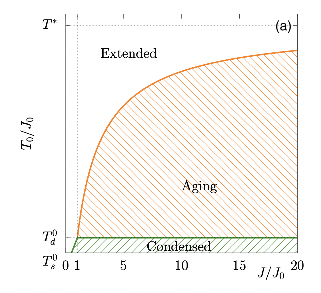
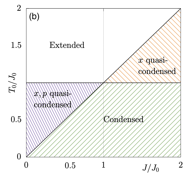
Figure 6: The dynamic phase diagram of the $p=3$ (a) and $p=2$ (b) isolated models. The initial conditions are drawn from the equilibrium Gibbs-Boltzmann distribution of the Hamiltonian ${\mathcal{H}}_{0}$ at inverse temperature $T_{0}$. The Hamiltonian evolution is performed with ${\mathcal{H}}$, differing from $H_{0}$ in a global rescaling of all couplings. The ratio $J/J_{0}$ measures the injection ($<1$) or extraction ($>1$) of energy at the quench.

6.2 The integrable two-body ($p=2$) case

This problem is almost quadratic and admits a very useful $N$ mode representation in which one focuses on the projection of the position and velocity vectors on the eigenvectors $\vec{v}_{\mu}$ of the interaction matrix ${\mathbb{J}}$: $x_{\mu}(t)=\vec{x}(t)\cdot\vec{v}_{\mu}$, $\dot{x}_{\mu}(t)=\frac{d{\vec{x}}(t)}{dt}\cdot\vec{v}_{\mu}$, with $\mu=1,\dots,N$. In condensed initial conditions at $T_{0}<T^{(0)}_{s}=J_{0}$, $\langle x_{\mu=N}\rangle_{i.c.}=(qN)^{1/2}$ and all other $\langle x_{\mu(\neq N)}\rangle_{i.c.}={\mathcal{O}}(1)$, while in extended ones at $T_{0}>T^{(0)}_{s}=J_{0}$ also $\langle x_{\mu=N}\rangle_{i.c.}$ is ${\mathcal{O}}(1)$.

This problem can be solved in two ways. First, one can simply integrate the Schwinger-Dyson Equations 12-14 with the kernels in Equations 15, $\eta=h=0$, $\gamma=1$ and $\overline{V}(q)=J^{2}q^{2}/2$. In this calculation, the average over the disorder ${\mathbb{J}}$ is done from the start. Second, one can proceed in a “mode resolved” and disorder dependent way. $N$ dynamic equations for the modes $x_{\mu}$ and $\dot{x}_{\mu}$, coupled via the spherical constraint, can be efficiently studied numerically. The most relevant projection is the one on the eigenvector associated to the eigenvalue at the edge of the spectrum, the $\mu=N$ one.

The dynamic phase diagram extracted from the combination of these two kinds of studies is depicted in Fig. 6(b). It is characterized by the Lagrange multiplier (which is simply related to the difference between the kinetic and potential energies) $z_{f}=\lim_{t\to\infty}z(t)$, the static susceptibility $\chi_{\rm st}=\lim_{t\to\infty}\chi(t_{1},0)=\lim_{t\to\infty}\int_{0}^{t_{1}}dt\,R(t_{1},t)$, the long time limit of the correlation with the initial condition $\lim_{t\to\infty}C(t,0)$, and the occupation of the largest mode as measured by $\langle x_{\mu=N}^{2}\rangle_{i.c.}$. From the analysis of the Schwinger-Dyson equations and the mode resolved dynamics we distinguished four phases:

1. For $T_{0}>T_{s}^{(0)}$ and $T_{0}>J$ an extended phase with $z_{f}=T_{0}+J^{2}/T_{0}$, $\chi_{\rm st}=1/T_{0}$, $C(t,0)\to 0$, $\langle x_{\mu=N}\rangle_{i.c.}=\langle p_{\mu=N}\rangle_{i.c.}=0$, and $\langle x_{\mu=N}^{2}\rangle_{i.c.}={\mathcal{O}}(1)$.

2. For $T_{0}>T_{s}^{(0)}$ and $T_{0}<J$ an extended phase with $z_{f}=2J$, $\chi_{\rm st}=1/J$, $C(t,0)\to 0$, and quasi condensation of $\langle x_{\mu=N}^{2}\rangle_{i.c.}={\mathcal{O}}(N^{1/2})$.

3. For $T_{0}<T_{s}^{(0)}$ initial conditions aligned along the $N$th eigenvector of the matrix ${\mathbb{J}}$ and $T_{0}<J$, one finds a condensed phase with $z_{f}=2J$, $\chi_{\rm st}=1/J$, $C(t,0)>0$, and $\langle x_{\mu=N}^{2}\rangle_{i.c.}=qN$ with $q={\mathcal{O}}(1)$.

4. For $T_{0}<T_{s}^{(0)}$ initial condition aligned along the $N$th eigenvector of the matrix ${\mathbb{J}}$ and $T_{0}>J$ a quasi-condensed phase of both $\vec{x}$ and $\vec{p}$ with $z_{f}=T_{0}+J^{2}/T_{0}$, $\chi_{\rm st}=1/T_{0}$, $C(t,0)\to 0$, and $\langle x_{\mu=N}^{2}\rangle_{i.c.}={\mathcal{O}}(N^{a})$ with $a<1$.

In phases 1. (extended), 2. (quasi condensed in $\vec{x}$) and 4. ($x$ and $p$ quasi condensed) a typical trajectory moves on the sphere and does not have a macroscopic projection on any of the Cartesian axes given by the eigenvectors of the interaction matrix ${\mathbb{J}}$, see Fig. 1(b). In phase 3., a typical trajectory starting from a symmetry broken initial condition with a macroscopic projection on the direction of the $N$th coordinate keeps this projection in the course of time and, typically, precedes around it. In none of these phases the quasi quadratic Neumann model equilibrates to a Gibbs-Boltzmann measure. Accordingly, there is no single temperature characterizing the values taken by different observables in the long time limits, not even after being averaged over long time intervals. Instead, in the infinite size limit, and after the Lagrange multiplier saturates to its asymptotic value $z_{f}$, the modes decouple, and each of them behaves as if in equilibrium at its own temperature $T_{\mu}$:

$$\overline{\langle p_{\mu}^{2}\rangle}_{i.c.}=k_{B}T_{\mu}\;,\qquad\qquad\quad\overline{\langle x_{\mu}^{2}\rangle}_{i.c.}=\frac{k_{B}T_{\mu}}{z_{f}-\lambda_{\mu}}\;.$$ (41)

The functional dependence of $T_{\mu}$ on the parameters is different in each phase. The co-existence of modes at different temperature is possible since they get effectively decoupled asymptotically.

Interestingly enough, the connection with the idea of measuring a time-delayed (or frequency) dependent effective temperature $T_{\rm eff}$ from the deviations from the fluctuation-dissipation relation of the global correlation, $C(t_{1},t_{2})=N^{-1}\sum_{\mu}[\langle x_{\mu}(t_{1})x_{\mu}(t_{2})\rangle_{i.c.}]$ and the corresponding linear response, then establishes very naturally [142, 143]. Each oscillator has its own frequency $\omega^{2}_{\mu}=(z_{f}-\lambda_{\mu})/m$. The global frequency dependent effective temperature is defined by $k_{B}\overline{T}_{\rm eff}(\omega)\equiv-\omega\tilde{C}_{\rm st}(\omega)/{\rm Im}\tilde{R}_{\rm st}(\omega)$, where the tildes indicate Fourier transform with respect to time delay. Setting the measuring frequency $\omega$ to $\omega_{\mu}$ one selects a particular mode and hence measures its own temperature, $\overline{T}_{\rm eff}(\omega=\omega_{\mu})=T_{\mu}$.

In the long-time limit the temporal averages coincide with the statistical ones calculated with a Generalized Gibbs Ensemble (GGE), [] Generalized Gibbs EnsembleAn extension of the canonical measure that includes all constants of motion in the exponential Boltzmann factor.

$$\rho(\{\dot{x}_{\mu},x_{\mu}\})={\mathcal{Z}}^{-1}(\{\gamma_{\mu}\})\;\;e^{-\sum_{\mu=1}^{N}\gamma_{\mu}I_{\mu}(\{\dot{x}_{\mu},x_{\mu}\})}\;.$$ (42)

The $I_{\mu}$ are the $N$ integrals of motion in involution, quartic functions of the phase space coordinates $\{x_{\mu},\dot{x}_{\mu}\}$ [144] parametrized by the post-quench eigenvalues $\lambda_{\mu}$ of ${\mathbb{J}}$:

$$I_{\mu}(\{\dot{x}_{\mu},x_{\mu}\})=x_{\mu}^{2}+\frac{m}{N}\sum_{\nu(\neq\mu)}\frac{(x_{\mu}{\dot{x}}_{\nu}-x_{\nu}{\dot{x}}_{\mu})^{2}}{\lambda_{\mu}-\lambda_{\nu}}\;,$$ (43)

The $\gamma_{\mu}$ are Lagrange multipliers which are fixed by the requirement,

$$\langle I_{\mu}\rangle_{\rm GGE}=I_{\mu}(0)\;,$$ (44)

with $I_{\mu}(0)$ the initial values right after the quench, which in any case are conserved by the dynamics. One then successfully verifies that, in all phases,

$$\overline{\langle p_{\mu}^{2}\rangle}_{i.c.}=\langle p_{\mu}^{2}\rangle_{\rm GGE}\;,\qquad\qquad\quad\overline{\langle x_{\mu}^{2}\rangle}_{i.c.}=\langle x_{\mu}^{2}\rangle_{\rm GGE}\;.$$ (45)

This is a particularly exciting integrable model for which one can tune the initial conditions to have radically different properties and also induce different kinds of phase transition with the quenches. The fact that the GGE describes its asymptotic dynamics was not granted a priori. The knowledge we had of its canonical equilibrium behaviour and relaxational dynamics were valuable guidelines to find the solution under Newton dynamics. It is to stress, though, that this is not a quadratic model because of the spherical constraint, and it is for this reason that it can support a non-trivial phase diagram.

7 DRIVEN DYNAMICS

Non-reciprocal interactions violate detail balance and inhibit equilibration. Specially interesting evolutions arise in glassy systems in the potential case and subjected to non-potential forces. On top of the possible currents generated, new hallmarks such as large number of attractors in the form of fixed points, limit cycles and chaotic evolutions may also exist. This Section deals with systems driven in different ways.

7.1 Rheology and active matter

Shearing, due to a non-conservative force applied on the boundaries of a system, is a common way of favoring the relaxation of glassy or jammed materials (shear thinning). This mechanical perturbation, which exerts work, can be mimicked with kernels $\Sigma$ and $D$, in Equations 12-14, that do not satisfy an FDT-like relation, that is $\Sigma\neq D^{\prime}R$. The relaxation time then decreases with the drive, $\tau_{\alpha}(\gamma)$, and this results in the suppression of the aging process at low temperatures. For forces of the $p$-body kind, such that in the absence of drive there is a glass transition mechanism, $C$ and $R$ are stationary but still display a two-step relaxation pattern, similar to the one observed at equilibrium slightly above $T_{d}$, if the perturbation is not too strong. In the weak drive limit, $C(t_{1},t_{2})=C_{\rm rapid}(t_{1}-t_{2})+C_{\rm slow}((t_{1}-t_{2})/\tau_{\alpha}(\gamma))$, with limiting values as the ones in Equations 24, 25, and violations of FDT consistent with a two-temperature scenario [21, 22]. Interestingly, the Monte Carlo simulation of these models with finite number of variables allows one to see jumps between the different metastable states that have long but finite lifetime. The non-potential forces let the system transit more easily over barriers and explore the landscape faster. Building upon the large $d$ formulation of the pure relaxational dynamics, Agoritsas et al. recently derived and studied the large $d$ equations that govern the dynamics of interacting particles under shear [145, 146].

Time-dependent drives also pump energy into a system. An example, relevant to describe vibrated granular matter [147] but also much studied quantum mechanically, is the one of a global periodic force, such as $h(t)=h\sin(\omega t)$. If the system is also connected to a thermal bath, it may reach a periodic “Floquet” regime, with monotonic stroboscopic behavior. The stemming dynamic phase diagram has three axes, $T/J$, $h/J$ and $\omega t_{0}$, with the frequency $\omega$ of the drive being another control parameter. For $p=2$ potentials, a critical line $h_{c}(\omega)$ going as $\omega^{1/4}$ for $\omega\sim 0$ at $T=0$, and increasing with $\omega$, was estimated. Below this curve aging with superimposed oscillations, that are washed out when observing stroboscopically at times $t_{n}=2\pi/\omega$, survives. In the $p=3$ case, the peculiar feature $\lim_{\omega\to 0}h_{c}(T/J,\omega)<h_{c}(T/J,\omega=0)$ was determined. The simulation of finite size systems with the periodic perturbation confirms the existence of metastable states that, however, do not block the dynamics completely. Jumps between these states are promoted by the injection of energy provided by the drive.

Yet another way to make a system time-translational invariant is to consider annealed disorder, that is change it slowly in time [148] with some time-scale $\tau_{\rm ann}$, which sets the structural relaxation time, and $C(t_{1},t_{2})\sim C_{\rm slow}((t_{1}-t_{2})/\tau_{\rm ann})$ for long time differences. One can also consider the coupling to several baths with different temperatures and characteristic times as a way of generating non-equilibrium dynamics [95]. [] Annealed disorderIt slowly changes in time.

Activity acts at the single particle level. A simple way to model it is to add random forces $h_{i}$ to the evolution equations, which are not accompanied by a corresponding dissipative term [149]. This is equivalent to adding $T\to\infty$ noise while keeping associated $\eta$ finite in Equations 1. The “bath” is then made of two components: a normal one in equilibrium at $T<\infty$ and a non-equilibrium one which does not satisfies FDT and drives the system out of equilibrium. A choice has been to use independent random forces with zero mean and exponentially decaying temporal correlations with a characteristic time-scale $\tau_{\rm act}$, which competes with the internal time-scale of the structural relaxation. While the equilibrium glass transition disappears in the presence of power dissipation of infinitesimally small amplitude [21], it survives the introduction of these fluctuating forces, even of large amplitude. Time correlation functions display a two-step decay reminiscent of the unforced behaviour. The location of the transition decreases for increasing driving. There is a non-equilibrium $T_{\rm eff}$ for the slow degrees of freedom even for the stationary fluid phase, not only deep into the glass [149]. The large $d$ description of active systems has also been addressed [150, 151].

7.2 Theoretical ecology

In theoretical ecology, coupled differential equations rule the time evolution of the population densities of different species in interaction which are, possibly, also coupled to an environment that can bring noise and immigration into the community. Recently, focus has turned to the analysis of ecosystems with large number of species, a limit in which statistical physics methods can be applied. Concrete examples of $N\gg 1$ communities range from microbes in the gut to plants in a rain forest. In their simplest modeling there is no spatial structure, an assumption justified for well-mixed ecosystems. The interactions are particularly difficult to infer in diversity-rich cases and are usually taken to be controlled by quenched random parameters. The similarity with disordered mean-field physical models then becomes apparent.

The population sizes $x_{i}$ are non-negative real variables that must remain so throughout the dynamics. If the absorbing value $x_{i}=0$ is reached at a given time, the population goes extinct and so remains subsequently if there is no immigration from the external world. A broad class of differential equations of the form $dx_{i}/dt=g_{i}(\vec{x})x_{i}$, with $\vec{x}=(x_{1},\dots,x_{N})$ and initial values $x_{i}(0)>0$ satisfy these conditions. [] Absorbing valueOnce reached it cannot be left.

7.2.1 Linear stability

A fundamental question in ecology is whether very diverse systems made of a large variety of interacting species are more resilient, or more unstable, than small size ones. The stability of such large complex systems can be quite generically studied using a linear set of equations, expected to represent the dynamics close to a fixed point, also named equilibrium in this context. Calling $y_{i}=x_{i}-x_{i}^{*}$ the deviation of the population density of the $i$th species from its equilibrium value $x_{i}^{*}$, the equations read

$$\frac{dy_{i}}{dt}=-\mu_{i}y_{i}+\sum_{k=1}^{N}J_{ik}y_{k}$$ (46)

for $i=1,\dots,N$, and $N$ the number of species. The parameters $\mu_{i}$ are positive and typically taken to be all equal to $\mu$. In the absence of interactions, $J_{ik}=0$ for all $i,k$, the system is self-regulating and any $y_{i}\neq 0$ returns to zero exponentially fast. The community matrix ${\mathbb{J}}$ has elements $J_{ik}$ and measures the per capita effect of the $k$th species on the $i$th one at the presumed equilibrium. Typically, it is a non-symmetric, $J_{ik}\neq J_{ki}$, square matrix.

Following previous numerical studies [152], May interpreted the $J_{ik}$ as the entries of a random matrix ${\mathbb{J}}$ with averaged number of non-vanishing elements, the averaged connectivity of the ecological network, equal to $C>0$ [153]. If species $k$ has no effect on species $i$, $J_{ik}=0$. Otherwise, the non-zero elements are independently sampled from a probability distribution with zero mean and variance $\sigma^{2}$. The assumption of there being as many positive as negative values of $J_{ik}$ is a plausible one for large ecosystems. Stability is ensured if all the eigenvalues of ${\mathbb{J}}$ have real parts less than $\mu$. Random matrix theory then establishes that in the large $N$ limit the system is almost certainly stable if $\mu/(\sigma\sqrt{CN})>1$ and unstable if $\mu/(\sigma\sqrt{CN})<1$, with a sharp transition between the two. For fixed $\mu$, the dynamics will almost certainly become unstable for sufficiently large $\sigma\sqrt{CN}$, that is for sufficiently large complexity as quantified by the connectivity and averaged interaction strength. The larger the system size, the more pronounced the effect, in the flavor of phase transitions. If, initially, the bound is violated, the ecosystem will drive some species to extinction until a stable community with a number of species satisfying the bound remains.

This surprising result was questioned since very diverse ecosystems, not satisfying this bound, do exist in Nature [154] (e.g. $N\sim 10^{5}$ for the oceanic plancton). The model has been enriched in many ways to avoid May’s restrictive limit [155, 156]. It is not the scope of this article to present a comprehensive review of theoretical ecology, it just means to illustrate how the methods and ideas of the non-equilibrium dynamics of disordered physical systems can be adapted to describe problems in this area.

A similar stability analysis can be applied to other areas, e.g. the functioning of neural networks [20, 157], systemic risk in trading [158], or large economies [159].

7.2.2 Instability: explosion of the number of fixed-points

Following the studies of rugged free-energy landscapes recalled in Sec. 4 the natural project to carry out for dynamical systems with random non-conservative forces $f_{i}$ is the enumeration and stability analysis of the fixed points. Fyodorov and Khoruzhenko went back to the evolution of the relative population sizes $x_{i}$’s and studied the model [23]

$$\frac{dx_{i}}{dt} = -\mu x_{i}+f_{i}(\vec{x})\qquad\mbox{with}\qquad f_{i}(\vec{x})=-\frac{\partial V(\vec{x})}{\partial x_{i}}+\sum_{k}\frac{\partial A_{ik}(\vec{x})}{\partial x_{k}}\;.$$ (47)

Each species becomes extinct on its own while the interactions, mimicked by the forces $f_{i}$, allow for the persistence of the community. The random forces are separated in potential and non-potential (divergence free) contributions. $V$ and $A_{ik}=-A_{ki}$ are statistically independent and Gaussian distributed, with $[V]=[A_{ik}]=0$, $[V(\vec{x})V(\vec{y})]=\nu^{2}\,\overline{V}(|\vec{x}-\vec{y}|^{2})$ and $[A_{ij}(\vec{x})A_{lm}(\vec{y})]=a^{2}N\,\overline{A}(|\vec{x}-\vec{y}|^{2})(\delta_{il}\delta_{jm}-\delta_{im}\delta_{jl})$.

The authors put the accent on the evaluation of the averaged number of zeroes of the total force, adapting the Kac-Rice method for counting solutions of simultaneous equations [56, 57] and using random matrix theory (annealed calculation). They found an abrupt transition at $\mu/(2\sigma\sqrt{N})=1$ with $\sigma=\sqrt{\nu^{2}+a^{2}}$ between a a phase with, on average, a single equilibrium and a non-trivial one with an averaged number of fixed points growing exponentially with $N$ [23] (for $a=0$ see [160]). This transition should be the reason for May’s instability. The vast majority of fixed points are unstable beyond it and, as explained below, induce long relaxation times and chaotic dynamics. At fixed $\nu^{2}/\sigma^{2}$, and decreasing $\mu/(2\sigma\sqrt{N})$ there is a new transition towards a phase with stable fixed points [161].

A similar explosion of complexity was measured in a neural network model [157], with randomly interconnected neural units with $f_{i}=\sum_{k(\neq i)}J_{ik}S(x_{k})$, $S$ an odd sigmoid function representing the synaptic non-linearity, and $J_{ik}$ independent Gaussian variables, representing the (non-symmetric) synaptic connectivity between neurons $i$ and $k$.

7.2.3 The random Lotka-Volterra model

A particular form of Equation 47 is

$$\frac{dx_{i}}{dt}=g_{i}(x_{i})-x_{i}\sum_{k(\neq i)}\alpha_{ik}x_{k}+\lambda_{i}\;.$$ (48)

$g_{i}(x_{i})$, describes the autonomous dynamics of species $i$ as if it were isolated from the rest, and decides whether it survives or disappears on its own. In the former case, after some relaxation time $x_{i}\to x_{i}^{*}$, the carrying capacity of the species. A common choice is $g_{i}(x_{i})=\frac{\mu_{i}}{K_{i}}x_{i}(K_{i}-x_{i})$ with zeros at $x^{*}_{i}=0$ (extinction) and $x^{*}_{i}=K_{i}$ (saturation). The second term in the right-hand-side models binary interactions, which could be generalized to include higher-body terms. The signs of $\alpha_{ik}$ represent the effects of one species on the other. If species $k$ is a predator of species $i$, $\alpha_{ik}$ is positive and tends to reduce the population $x_{i}$. If the two species compete for the same resources, both $\alpha_{ik}$ and $\alpha_{ki}$ are positive. Both are negative if there is mutualism. $\lambda_{i}$ is an immigration rate which is usually taken to be uniform across species, $\lambda_{i}=\lambda$. In the spirit of May’s approach, the coefficients $\alpha_{ik}$ are taken to be i.i.d. random variables. In the simplest description all species are connected to all others and the moments are $[\alpha_{ik}]=\alpha/N$, $[(\alpha_{ik}-[\alpha_{ik}])^{2}]=\sigma^{2}/N$ and $[(\alpha_{ik}-[\alpha_{ik}])(\alpha_{ki}-[\alpha_{ki}])]=\gamma\sigma^{2}/N$. The scaling with $N$ ensures a proper large $N$ limit. The parameter $\gamma$ measures the asymmetry of the interactions; it ranges from $-1$ (fully antisymmetric, all interactions are of predation-prey type) to $1$ (fully symmetric, an energy can be defined). A linear expansion around a putative fixed point $x_{i}^{*}$ yields May’s Equation 46 with a simple relation between $\mu$, ${\mathbb{J}}$, $g_{i}$ and the $\alpha_{ik}$. Finally, one could add demographic noise accounting for deaths, births, and other unpredictable events. It is usually chosen to be a Gaussian random variable with zero mean and

$$\langle\xi_{i}(t_{1})\xi_{j}(t_{2})\rangle=2T\,x_{i}(t_{1})\,\delta_{ij}\delta(t_{1}-t_{2})\;.$$ (49)

The multiplicative form of Equations 48-49. ensures that for $\lambda_{i}=0$ if the absorbing value $x_{i}=0$ is reached the population goes extinct and $x_{i}$ remains zero at all later times. The noise is treated in the Ito convention [41, 162, 163, 164, 165, 166].

The model has five control parameters: the average strength $\alpha$ and the variety $\sigma$ of the interactions, their asymmetry $\gamma$, the immigration rate $\lambda$ and the temperature $T$ of the demographic noise. In the $N\to\infty$ limit, the single variable equations are [41, 164]

$$\frac{dx(t_{1})}{dt_{1}}=x(t_{1})\left[1-x(t_{1})-\alpha m(t_{1})-\sigma\zeta(t_{1})+\gamma\sigma^{2}\int_{0}^{t_{1}}\!\!dt\,R(t_{1},t)x(t)+h(t)\right]$$ (50)

with the averaged population, self correlation and linear response

$$m(t_{1})=[\langle x(t_{1})\rangle]\,,\quad C(t_{1},t_{2})=[\langle x(t_{1})x(t_{2})\rangle]\,,\quad R(t_{1},t_{2})=[\langle\left.\frac{\delta x^{(h)}(t_{1})}{\delta h(t_{2})}\right|_{h=0}\!\!\!\!\rangle]\,,$$ (51)

where the angular brackets denote average over initial conditions and the effective noise $\zeta(t_{1})$ with zero mean and self-consistent correlations $\langle\zeta(t_{1})\zeta(t_{2})\rangle=\langle x(t_{1})x(t_{2})\rangle$. For the sake of compactness we set the demographic noise and the immigration rate to zero and we absorbed $\mu_{i}$ and $K_{i}$ in a redefinition of the $x_{i}$. Importantly enough, the original system (with no demographic noise) was deterministic, but the effective single variable one is stochastic. The fully-connected model without demographic noise at fixed $\gamma$ has three phases [163, 41]:

1. Single fixed point for small $\sigma$. In the long time limit, all initial conditions reach the same saturation values, $x_{i}^{*}$ (some $x_{i}^{*}$ may vanish if the $i$th species goes extinct). The $x_{i}^{*}$ are Gaussian distributed, truncated at negative values. This state is stable against local and global perturbations. The global correlation functions are stationary.

2. Multiple Attractors for large $\sigma$ and small immigration rate $\lambda\stackrel{{\scriptstyle>}}{{\sim}}0$. The single stable fixed point loses its stability at $\sigma_{c}=\sqrt{2}/(1+\gamma)$, and not only the averaged but even the typical number of equilibria grows exponentially with the number of species [167]. The system cannot settle in a fixed point and this phase exhibits chaotic dynamics, with large fluctuations of the species populations, for $\gamma\neq 1$ or aging dynamics, as for physical systems, for $\gamma=1$. Chaos is self-destructive for $\lambda=0$. Similar features were observed in neural networks [20], evolutionary game theory [168, 169] and replicator equations with nearly antisymmetric random interactions [165]. [] Chaotic dynamicsThe populations do not stabilize and undergo large fluctuations.

3. Multiple Attractors for large $\sigma$ and vanishing immigration rate $\lambda=0$. The system ages with a rather different mechanism from the one of the physical $p$-body models which do not have absorbing boundary values. Here there are near-extinction processes, whereby some population sizes go very close to zero for some time before rebounding, accompanied by a global slowdown of the dynamics. Asymptotically, the time it takes for a variable to leave the vicinity of an absorbing value to visit the vicinity of another is proportional to the age of the system. This mechanism was coined aging by near extinctions [170] and it is due to the fact that all the fixed points are unstable [171], contrary to the marginal threshold reached in usual glassy dynamics [31]. [] Aging by near extinctionsThe progressive dynamic slowdown due to the approach to unstable fixed points.

4. Unbounded Growth for large negative $\alpha$. In this case the interactions are so cooperative that the dynamics can override the single-species saturation. The unbounded growth is a pathology which could be cured by a stronger saturation imposed by $g_{i}(x_{i})$. For instance, a cubic term of the form $g(x_{i})=-\mu_{i}x_{i}(1-x_{i}/K_{i})(x_{i}-m_{i})$ avoids the unbounded growth but it also drastically changes the phase diagram [172].

In these explicitly out of equilibrium dynamics the deviations from the standard FDT have not been characterized yet. It remains, certainly, as an interesting open problem that should be at reach of the numerical analysis.

Another issue concerns the effects of demographic noise [166]. At fixed $\gamma$, $\alpha$ and $\lambda$, the phase diagram, parametrized by temperature and the species variability $\sigma$, has three phases. In the symmetric case $\gamma=1$, one phase has a single fixed point in which the relaxation time is finite and the correlation decays as a function of time difference. Another one has multiple attractors and the relaxation ages, similarly to what is found in glassy systems. Finally, a phase in which the multi-equilibria are organized in a hierarchical manner (a.k.a. Gardner phase) exists at still lower temperatures. When the asymmetry is considered, the dynamics in the multi-attractor phases become chaotic and it has an indefinitely long lifetime for $\lambda>0$, while it is replaced by aging for $\lambda=0$.

7.3 Optimization and learning

How to identify the absolute minimum of a function defined on a high dimensional space is the key issue in hard optimization problems. Usually, the algorithms used to attain this goal are based on physical rules. Popular choices are Langevin dynamics satisfying detailed balance, or Monte Carlo rules also respecting this condition. Such evolutions eventually minimize the energy or cost function of a finite size system if the zero temperature limit is taken in a convenient way. However, this strategy can be very inefficient for systems with complex free-energy landscapes, needing a number of operations that scale as the exponential of system size. Alternatives have been searched for since long ago. In simulated annealing, cluster Monte Carlo methods and other, the physical restrictions are lifted. In this section we briefly mention some of the recent progress in this direction.

Langevin dynamics with divergence-less forces which do not respect detailed balance, have been proposed to accelerate the diffusive dynamics while respecting the asymptotic statics measure [173, 174, 175]. While the dynamics pf $p$-body models are indeed accelerated, with times rescaled by a factor, the dynamic transition at $T_{d}$ is not modified [176]. Basically, there is an enhanced mobility which accelerates the evolution without affecting the free-energy landscape.

Understanding the extraordinary performance of artificial neural networks, in the deep learning or perceptron realization, is of extreme importance. The perceptron [177, 178] is a simple model of a natural or artificial neuron: [] PerceptronA model neuron. it receives an input, and once multiplied by the learned weight coefficient, generates an output. In machine learning, networks of such perceptrons are used as classifiers. The feed-forward networks, at the basis of modern deep neural networks, are made of successive layers of such neurons. [] Deep neural networksFeed-forward networks with many internal layers. The perceptron problem consists in, given a set of inputs and another set of associated outputs, find the synaptic weights, connections and strengths, such that the network makes a correct classification. Training a network with supervised learning corresponds to minimizing a cost function that depends on the parameters of the network and the dataset. The latter can also be seen as a constraint satisfaction problem: [] Constrained satisfaction problemsrequire the variables to satisfy a set of constraints. how to determine the synaptic weights that let all input-output constraints be satisfied simultaneously. Deep neural networks are able to extract high-level features from data and thus be notably efficient in the classification tasks. In the random perceptron the inputs and associated outputs are taken to be uncorrelated random variables [179]. If, moreover, the synaptic variables are spherically constrained, the zero capacity corresponds to a satisfiability/unsatisfiability threshold which is analogous to the jamming transition of hard-spheres in very high dimensions. The Schwinger-Dyson equations ruling the Langevin dynamics of a spherical random perceptron, with the same structure as Equations 12-14 have been established in [39]. The relation between the kernels $\Sigma$ and $D$ and the global correlation and linear response $C$ and $R$ are much more complicated than the simple algebraic ones of the $p$ body model. A complete analytic and numerical solution of this problem is not available yet but constitutes an interesting open problem.

The supervised learning dynamics of a deep neural network shares similarities but also differs from the relaxation of the spherical $p\geq 3$ body model [180]. [] Supervised learninguses a training set to teach the network to yield the desired output. In an over-parametrized deep neural network, in which the number parameters exceeds the size of the training dataset, three regimes were identified: an initial exploration of the energy/loss landscape, followed by a decrease of the loss in which the system displays aging dynamics, and a final almost stationary and diffusive regime in which the network reaches the bottom of the landscape. Barrier crossing does not seem to play a role in the learning process while slow evolution along flat directions does. Instead, in under parametrized networks the loss function approaches a non-vanishing value, there is aging, and the relaxation resembles strongly the one of the spherical $p\geq 3$ model.

A Langevin algorithm intended to sample the posterior probability measure for the spiked mixed matrix-tensor model, and its representation in terms of Schwinger-Dyson equations, was presented and studied in detail in [181, 182]. This problem is very similar to the mixed $p+2$ model discussed in Sec. 5.1.3.

Gradient descent is typically used to train a network, but this requires the evaluation of the state of the neural weights on the full training set. [] Stochastic gradient descentEvaluates the gradient on a subset of the training set. Stochastic gradient descent approximates the gradient by evaluating it only on a small subset of the training set (batch), changed at each step of the dynamics. Networks trained this way have an excellent performance, and can even generalize, that is, classify correctly previously unseen data. [] Generalizationthe ability to classify correctly previously unseen data. The choice of different batches introduces noise on the otherwise deterministic gradient descent. Understanding the nature of this noise is a hot topic. This microscopic dynamics bear similarities with the ones of physical systems, where the stochastic dynamics of the degrees of freedom is dressed with local and independent forcing variables (strain deformation in driven systems and self-propulsion in active matter). Several stochastic gradient descent algorithms which achieve a binary classification of Gaussian mixtures were studied in this setting [183, 184]. The $C$ and $R$ of the network weights can then be calculated [184] and, more importantly, compared so as to extract a $T_{\rm eff}$ from the deviations from the FDT [78]. In the under-parametrized or un-satisfiable phase where the network cannot achieve zero training error, the dynamics go to a stationary state with a finite $T_{\rm eff}$ with a non-monotonic dependence on the batch size. Instead, in the over-parametrized or satisfiable phase the dynamics stop at one solution with zero training error, and $T_{\rm eff}$ approaches zero asymptotically, consistently with the idea that stochastic gradient descent implements a self-annealing procedure. Reference [184] discusses the behavior of $T_{\rm eff}$ in several improvements upon the simplest stochastic gradient descent algorithm as well.

8 QUANTUM DYNAMICS

Disorder and interactions lead to the very rich phenomena discussed so far. Adding quantum fluctuations amplifies the palette of intriguing phenomena even more so [185].

8.1 Statics and dynamics in $p$ models

Two parameters control the canonical equilibrium properties of quantum models with Hamiltonian $\hat{\mathcal{H}}=\hat{K}+\hat{V}$. One quantifies thermal fluctuations and it is the traditional temperature over the interaction strength $J$. The other one measures the strength of quantum fluctuations and can be organized in the adimensional form $\Gamma=\hbar^{2}/(mJ)$.

The $p$ body models have a static phase diagram with ordered and disordered phases. The order of the phase transition depends on the type of interactions considered. It is continuous for $p=2$, while it has a mixed RFOT/truly first order transition for $p\geq 3$. The former applies close to the classical limit, while the latter close to the quantum critical point. These conclusions have been drawn from the replica analysis [186, 187] which, on top of the usual order parameter in the form of an overlap matrix in replica space $Q_{ab}$, includes an imaginary time dependent one $Q_{aa}(\tau)=N^{-1}[\langle\sum_{i=1}^{N}{\rm T}\hat{x}^{a}_{i}(\tau)\hat{x}^{a}_{i}(0)\rangle]=q_{d}(\tau)$. (The average represents $\langle\dots\rangle={\rm Tr}(\hat{\rho}\dots)/{\rm Tr}\hat{\rho}$, with $\hat{\rho}$ the equilibrium density operator at inverse temperature $\beta$, $a,b=1,\dots,n$ are replica indices, $\tau$ is the periodic imaginary time and ${\rm T}$ the time ordering operator.) This function is determined by the equation

$$G_{0}^{-1}(\tau)q_{d}(\tau)=\delta(\tau)+\int_{0}^{\tau}d\tau^{\prime}\,\Sigma(\tau-\tau^{\prime})q_{d}(\tau^{\prime})\;,$$ (52)

with $G_{0}^{-1}(\tau)=m\partial_{\tau}^{2}+z(\tau)$, $\Sigma=-J^{2}/(2\hbar)\,q_{d}^{p-1}$, and $q_{d}(0)=q_{d}(\beta\hbar)$. Close to the quantum critical point $(T=0,\Gamma_{\rm Q})$ of the $p\geq 3$ model some off-diagonal elements of the replica matrix, $Q_{ab}=N^{-1}\sum_{i=1}^{N}[\langle{\rm T}\hat{x}^{a}_{i}x^{b}_{i}\rangle]$ with $a\neq b$, jump from zero to a finite value, and this implies that the ground states on the two sides of the transition are essentially unrelated [186, 187].

Also interesting is to consider the effect of the coupling to a an ensemble of quantum harmonic oscillators with spectral density $I(\omega)$. It manifests in the addition of a bath induced term to the self-energy $\Sigma$ which in Fourier space reads $\tilde{\Gamma}_{R}(\omega)\propto\omega^{s}$ with Ohmic ($s=1$), super ($s>1$) and sub ($s<1$) Ohmic possibilities encoded in this compact form. Their effect is highly non-trivial as it can make the ordered phase more stable, and thus occupy a larger portion of the phase diagram [188].

The concept of a free-energy landscape can also be applied to a system with quantum fluctuations [189]. Its properties, as $T/J$ and $\Gamma$ are varied, can be studied with similar techniques to the ones used to analyze the classical landscape, with the addition of the imaginary-time dependence of $q_{d}(\tau)$. In the $p\geq 3$ model case, a complex landscape with large multiplicity of saddles of all kinds subsists under quantum fluctuations.

The relaxation of a quantum mean-field disordered model in contact with a quantum bath is still governed by Schwinger-Dyson equations like the ones in Equations 12-14 although with some subtle differences [190, 191]. Firstly, $G_{0}^{-1}(t_{1})=m\partial_{t_{1}}^{2}+z(t_{1})$ is a second order differential operator. Secondly, a quantum bath gives rise to retarded contributions to the self-energy and vertex $\Sigma$ and $D$ that replace the terms proportional to $\eta$ in Equations 12-14 (but do not depend on $C$ and $R$). They read The explicit coupling to a quantum bath adds to this equation two extra time-delayed terms

$$\Gamma_{R}(t_{1}-t_{2}) = -\theta(t_{1}-t_{2})\int_{0}^{\infty}d\omega\,I(\omega)\,\sin[\omega(t_{1}-t_{2})]\;,$$ (53)

$$\Gamma_{C}(t_{1}-t_{2}) = \int_{0}^{\infty}d\omega\,I(\omega)\,\coth\left(\frac{1}{2}\beta\hbar\omega\right)\,\cos[\omega(t_{1}-t_{2})]\;.$$ (54)

Thirdly, the part of the kernels $\Sigma$ and $D$ due to the interactions are not as simple as the ones in Equations 15. For the model with $p$-body interactions they read

$$\Sigma=-\frac{J^{2}p}{\hbar}\,{\rm Im}\left(C-\frac{{\rm i}\hbar}{2}R\right)^{p-1}\!\!\!\!\!,\qquad\qquad D=\frac{J^{2}p}{2}\,{\rm Re}\left(C-\frac{{\rm i}\hbar}{2}R\right)^{p-1}\!\!\!\!\!.$$ (55)

Equilibrium initial conditions at inverse temperature $\beta_{0}$ can also be imposed. To do it, one needs to introduce correlations living on the imaginary time axis and, moreover, correlations that mix real and imaginary times. In the end, the terms proportional to $J_{0}/T_{0}$ in Equations 12-14 are replaced by integral terms involving these functions, with the addition of equations that govern their real and imaginary time evolutions. In particular, an equation like 52 determines the evolution of $q_{d}(\tau)$ with the periodic boundary condition $q_{d}(\beta_{0}\hbar)=q_{q}(0)$ fixed by the initial temperature. The full set of Schwinger-Dyson equations is considerably more complicated than the one for the classical case [34], which is recovered by taking $\hbar\to 0$. Finally, let us mention that the quantum $p$-spin model can also be connected to the Mode-Coupling description of super-cooled quantum liquids [192].

The solution to the Schwinger-Dyson equations was first derived in a limit in which the coupling to the bath is taken to be so weak that it does not modify the location of the phase transitions. It shows similarities and differences with the classical ones [190, 191]. First of all the second-order differential operator induces oscillations, the frequency of which depend on the control parameters. In consequence, after quenches from disordered initial conditions to parameters that are not too far from the ordered phase or within it, the $C$ and $R$ at short time differences (high-frequency dynamics) depend on $\Gamma$. In particular, there are oscillations in $t_{1}-t_{2}$ that smoothly decay in amplitude as the plateau is approached. Instead, these functions at long time differences (low-frequency dynamics) are monotonic and qualitatively identical to those of their classical counterparts. For $p\geq 3$ models, the quenched dynamics in the ordered phase hovers over saddles in the free-energy landscape and slowly relaxes its energy, as in the weak ergodicity breaking scenario, with aging. The quantum FD relation is the equilibrium one on short time differences but takes the classical form, with an effective temperature $T_{\rm eff}$ that exceeds the one of the bath (even at $T=0$). The generation of a $T_{\rm eff}>0$ “decoheres” the dynamics renders this regime classical. The dynamical phase transition precedes the thermodynamic one also quantum mechanically. The effect of the bath is highly non-trivial as it can enlarge the extent of the ordered phase in the phase diagram [188]. One can also tune the initial state to be within one of the valleys in the free-energy landscape and show that the subsequent dynamics remains confined to it (at least for times which are not exponentially large in system size) [34, 193]. Because of the first order phase transition of the $p\geq 3$ systems, quantum annealing is not expected to be useful for them [194, 195] which are, however, the ones that one would wish to optimize since they are related to the celebrated $K$-satisfiability optimization problem [65, 196].

8.2 Many-body localization

Quantum glassiness and many-body localization have been related to each other in recent years. However, they are important differences between the two phenomena.

Non-interacting quantum particles in one dimension under a disordered potential Anderson localize and stop diffusing on the scale of the elastic mean-free path. Many-body localization (MBL) is its interacting counterpart [197]. It relies on the discreteness of non-interacting excitations and the rareness of resonant interactions, which then fail to induce diffusion of energy. MBL can only occur in isolation, with no coupling to the continuum of a bath which would reinstate transport and ergodicity. In contrast, glassy phases are stable against a bath, as they rely on the rugged structure of the free-energy landscape. Moreover, MBL phases are highly susceptible to local inclusions where disorder is weak, which inhibit it in high dimensions and may even destroy it completely (the fate of MBL in 1d is a subject of debate). In contrast, glasses, like standard symmetry broken phases, are rendered more stable in high $d$. In short, both quantum glassiness and MBL entail non-ergodicity and impede full thermalization but they do so for fundamentally different reasons.

8.3 The SYK model

Kitaev proposed to use the $p=4$ potential where the operators $\hat{x}_{i}$ are replaced by Majorana fermions as a toy model for near-extremal black holes [106]. The relevant correlation is $q_{d}(\tau)=-N^{-1}\sum_{i=1}^{N}[\langle{\rm T}\hat{\psi}_{i}(\tau)\hat{\psi}_{i}(0)\rangle]$, and satisfies Equation 52 with $G_{0}^{-1}=d_{\tau}$ and $\Sigma=J^{2}q_{d}^{3}$. The main reason to claim a connection with gravity in a nearly AdS₂ background is that this model is not glassy, but becomes approximately conformal after dropping time-derivatives, in the low-frequency limit, with a time-reparametrization symmetry which is broken to SL(2,R). A sigma model describing the cost of reparametrizations in terms of a Schwarzian action was constructed [198], similarly to what was done in [104, 199] for the time-reparametrizations in glassy models. The model shares also two thermodynamic properties of such black holes: it has non-zero entropy as $T\to 0$ (after $N\to\infty$) and a linear in $T$ specific heat. Kitaev’s model is very close to the model proposed by Sachdev and Ye to describe non-Fermi liquid behavior in condensed matter systems [105], and was thus dubbed SYK. A discussion of more connections between the SYK and glassy models with a RFOT can be found in [200].

The SYK model is a maximally chaotic/perfect scrambler meaning that the bound $\lambda_{T}\leq 2\pi T/\hbar$ on the Lyapunov exponent $\lambda_{T}$ (a consequence of the FDT [201, 202]), defined from the exponential growth of out-of-time-order correlations [203, 198], is saturated. This kind of chaos was then studied in the disordered and marginal glassy phases of the spherical $p$ models [204, 205]. Quantum fluctuations were found to make the disordered phase less and the glassy phase more chaotic. In the classical limit $\hbar\to 0$ a crossover from strong to weak chaos, as marked by a maximum in $\lambda_{T}$, arises well above $T_{d}$, concomitant with the onset of two-step slow relaxations. Finally, we comment that the experiment of setting two systems in contact, commonly performed in studies of disordered systems, see e.g. [206, 78], has, in this context, the interpretation of creating a wormhole between the two spaces.

9 CONCLUSIONS

We discussed a number of classical systems, made up of a large number of degrees of freedom, with stochastic or Newtonian dynamics influenced by a very rough free-energy landscape, or complex quenched random forces. All this leads to uncommon phases and even more unusual dynamics. Their quantum extensions are equally rich.

The models we dealt with may seem artificial for physical applications. Still, they provide a successful mean-field description of coarsening, glassiness, and jamming. Their limitations to capture the full behavior of finite dimensional physical systems have been identified and efforts are being made to overcome them. The same models are the actual problems one needs to understand in other fields of science, such as optimization, artificial intelligence, and ecology. The enormous amount of knowledge gathered by the statistical physics community can now be exploited in these other areas.

Some important and generic notions that came out of the analytic solution of the fully-connected models are rugged free-energy landscapes, marginally stable regions, critical slowing down, weak and strong ergodicity breaking, weak long-term memory, aging, violations of the fluctuation-dissipation theorem, effective temperatures, time reparametrization invariance, soft modes and dynamic fluctuations, Generalized Gibbs Ensembles, multiple fixed points, and chaos. They all appear in one way or another in the problems discussed here. Some of them were known beforehand but others not. Once uncovered in this idealized theoretical context, they were explored, and in some cases confirmed, numerically and experimentally in more realistic physical systems.

Many open issues remain to be solved. The complete understanding of models with even more complex free-energy landscapes than the ones with monomial $p$ potentials is lacking. An efficient algorithm able to solve the generic self-consistency single-variable equations for the $d\to\infty$ problems, when no stationarity hypothesis can be used, is not available yet. All analytic results were derived having taken the limit $N\to\infty$ from the start, and eventually considering the long-times asymptotic. The sharp dynamic transitions thus predicted cannot exist for finite size systems or in finite dimensions and should be replaced by a crossover. Having said so, the analytic description of this process, and the eventual approach to equilibrium appears as a formidable task and has remained elusive since the derivation of the $N\to\infty$ solution.

DISCLOSURE STATEMENT

The authors are not aware of any affiliations, memberships, funding, or financial holdings that might be perceived as affecting the objectivity of this review.

References

- [1] Hohenberg PC, Halperin BI. 1977. Rev. Mod. Phys. 49:435
- [2] Bray AJ. 1994. Adv. Phys. 43:357
- [3] Onuki A. 2004. Phase transition dynamics. Cambridge University Press
- [4] Puri S, Wadhawan V, eds. 2009. Kinetics of phase transitions. Taylor and Francis Group
- [5] Henkel M, Pleimling M. 2010. Non-equilibrium phase transitions: ageing and dynamical scaling far from equilibrium. Springer-Verlag
- [6] Berthier L, Biroli G. 2011. Rev. Mod. Phys. 83:587
- [7] Bloch I, Dalibard J, Zwerger W. 2008. Rev. Mod. Phys. 80:885
- [8] Duran J. 1999. Sands, powders, and grains: An introduction to the physics of granular materials. New York: Springer-Verlag
- [9] Bechinger C, Leonardo RD, Löwen H, Reichhardt C, Volpe G, Volpe G. 2016. Rev. Mod. Phys. 88:045006
- [10] Azaele S, Suweis S, Grilli J, Volkov I, Banavar JR, Maritan A. 2016. Rev. Mod. Phys. 88:035003
- [11] Bahri Y, Kadmon J, Pennington J, Schoenholz S, Sohl-Dickstein J, Ganguli S. 2019. Ann. Rev. Cond. Matt. 11:501
- [12] Krzakala F, Ricci-Tersenghi F, Zdeborová L, Tramel EW, Zecchina R, Cugliandolo LF, eds. 2013. Statistical physics, optimization, inference, and message-passing algorithms. Lecture Notes of the Les Houches School of Physics. Oxford: Oxford University Press
- [13] Naumann-Woleske K, Knicker MS, Benzaquen M, Bouchaud JP. 2023. Exploration of the parameter space in macroeconomic agent-based models. Handbook of Complexity Economics
- [14] Cugliandolo LF. 2002. Dynamics of glassy systems. ArXiv:cond-mat/0210312
- [15] Cavagna A. 2009a. Phys. Rep. 476:51
- [16] Montanari A, Sen S. 2022. A short tutorial on mean-field spin glass techniques for non-physicists. ArXiv:2204.02909
- [17] Folena G, Manacorda A, Zamponi F. 2022. Introduction to the dynamics of disordered systems: equilibrium and gradient descent. ArXiv:2202.02413
- [18] Mézard M, Parisi G, Virasoro MA. 1986. Spin glass theory and beyond: An introduction to the replica method and its applications. Singapore: World Scientific
- [19] Crisanti A, Sommers HJ. 1992. Z. Phys. B: Cond. Matter 87:341
- [20] Sompolinsky H, Crisanti A, Sommers HJ. 1988. Phys. Rev. Lett. 61:259
- [21] Cugliandolo LF, Kurchan J, Le Doussal P, Peliti L. 1997. Phys. Rev. Lett 78:350
- [22] Berthier L, Barrat JL, Kurchan J. 2000. Phys. Rev. E 61:5464
- [23] Fyodorov YV, Khoruzhenko BA. 2016. Proc. Nat. Acad. Sc. 113:6827
- [24] Hofbauer J, Sigmund K. 1998. Evolutionary games and population dynamics. Cambridge University Press
- [25] Martin PC, Siggia ED, Rose HA. 1973. Phys. Rev. A 8:423
- [26] Janssen HK. 1976. Z. Phys. B Con. Matt. 23:377
- [27] De Dominicis C. 1976. J. Phys. Colloques C1:37
- [28] Arnoulx de Pirey T, Cugliandolo LF, Lecomte V, van Wijland F. 2023. Path integrals and stochastic calculus. Arxiv:2211.09470. Adv. Phys. (to appear).
- [29] Bouchaud JP, Cugliandolo LF, Kurchan J, Mézard M. 1996. Physica A 226:243
- [30] Sompolinsky H, Zippelius A. 1981. Phys. Rev. Lett. 47:359
- [31] Cugliandolo LF, Kurchan J. 1993. Phys. Rev. Lett. 71:173
- [32] Barrat A, Burioni R, Mézard M. 1996. J. Phys. A: Math. Gen. 29:L81
- [33] Cugliandolo LF, Lozano GS, Nessi N. 2017. J. Stat. Mech 2017:083301
- [34] Cugliandolo LF, Lozano GS, Nessi N. 2019. J. Stat. Mech 2019:023301
- [35] Schwinger J. 1961. J. Math. Phys. 2:407
- [36] Keldish LV. 1964. Zh. Eksp. Teor. Fiz. 47:1515
- [37] Stefanucci G, van Leeuwen R. 2013. Nonequilibrium many body theory of quantum systems. Cambridge: Cambridge University Press
- [38] Chakraborty A, Gorantla P, Sensarma R. 2019. Phys. Rev. B 99:054306
- [39] Agoritsas E, Biroli G, Urbani P, Zamponi F. 2018. J. Phys. A: Math. Theor. 51:085002
- [40] Ben Arous G, Dembo A, Guionnet A. 2006. Probability Theory and Related Fields 136:619
- [41] Roy F, Biroli G, Bunin G, Cammarota C. 2019. J. Phys. A: Math. Theor. 52:484001
- [42] Georges A, Kotliar G, Krauth W, Rozenberg MJ. 1996. Rev. Mod. Phys. 68:13
- [43] Ros V, Fyodorov Y. 2023. The high-d landscapes paradigm: spin-glasses, and beyond. Singapore: World Scientific. ArXiv:2209.07975
- [44] Auffinger A, Montanari A, Subag E. 2023. Optimization of random high-dimensional functions: Structure and algorithms. Singapore: World Scientific. ArXiv:2206.10217
- [45] Kosterlitz JM, Thouless DJ, Jones RC. 1976. Phys. Rev. Lett 36:1217
- [46] Bray AJ, Moore MA. 1980. J. Phys. C 13:L469
- [47] Kurchan J, Parisi G, Virasoro MA. 1993. J. Phys. I 3:1819
- [48] Crisanti A, Sommers HJ. 1995. J. Phys. I 5:805
- [49] Monasson R. 1995. Phys. Rev. Lett. 75:2847
- [50] Cavagna A, Giardina I, Parisi G. 1998. Phys. Rev. B 57:11251
- [51] Cavagna A, Garrahan JP, Giardina I. 1999. J. Phys. A: Math. Gen. 32
- [52] Kirkpatrick TR, Thirumalai D. 1987. Phys. Rev. B 36:5388
- [53] Debenedetti P. 1996. Metastable liquids: Concepts and principles. Princeton Univ. Press
- [54] Kirkpatrick TR, Thirumalai D. 2015. Rev. Mod. Phys. 87:183
- [55] Wolynes PG. 2023. The random first order transition theory of glasses in real space-time: Instantons, strings, flames and flows. Singapore: World Scientific
- [56] Kac M. 1943. Bull. Amer. Math. Soc. 49:314
- [57] Rice SO. 1944. Bell System Tech. J. 23:282
- [58] Ros V, Ben Arous G, Biroli G, Cammarota C. 2019. Phys. Rev. X 9:011003
- [59] de Dominicis C, Young AP. 1983. J. Phys. A 16:2063
- [60] Gradenigo G, Angelini MC, Leuzzi L, Ricci-Tersenghi F. 2020. J. Stat. Mech. 2020:113302
- [61] Franz S, Parisi G. 1995. J. Phys. I France 5:1401
- [62] Gardner E. 1985. Nucl. Phys. B 257:747
- [63] Charbonneau P, Kurchan J, Parisi G, Urbani P, Zamponi F. 2014. Nat. Commun. 5:3725
- [64] Altieri A, Biroli G, Cammarota C. 2020. J. Phys. A: Math. Theor. 53:375006
- [65] Monasson R, Zecchina R. 1997. Phys. Rev. E 56:1357
- [66] Rizzo T, Yoshino H. 2006. Phys. Rev. B 73:064416
- [67] Barrat A, Franz S, Parisi G. 1997. J. Phys. A 30:5593
- [68] Capone B, Castellani T, Giardina I, Ricci-Tersenghi F. 2006. Phys. Rev. B 74:144301
- [69] Crisanti A, Leuzzi L. 2006. Phys. Rev. B 73:014412
- [70] Barbier D, Cugliandolo LF. 2020. J. Stat. Mech. 2020:063207
- [71] Auffinger A, Zhou Y. 2022. The spherical p+s spin glass at zero temperature. ArXiv:2209.03866
- [72] Folena G, Franz S, Ricci-Tersenghi F. 2020. Phys. Rev. X 10:031045
- [73] Folena G, Franz S, Ricci-Tersenghi F. 2021. J. Stat. Mech. 2021:033302
- [74] Cugliandolo LF, Dean DS. 1995a. J. Phys. A: Math. Gen. 28:4213
- [75] Calabrese P, Gambassi A. 2005. J. Phys. A 38:R133
- [76] Cugliandolo LF, Dean DS. 1995b. J. Phys. A: Math. Gen. 28:L453
- [77] Middleton C. 2022. Physics Today 75:14
- [78] Cugliandolo LF, Kurchan J, Peliti L. 1997. Phys. Rev. E 55:3898
- [79] Scherer GW. 1986. Relaxation in glass and composites. New York: Wiley
- [80] Bouchaud JP. 1992. J. Phys. I (France) 2:1705
- [81] Kim BS, Latz A. 2001. EPL 53:660
- [82] Cugliandolo LF, Le Doussal P. 1996. Phys. Rev. E 53:152
- [83] Kurchan J, Laloux L. 1996. J. Phys. A: Math. Gen. 29:1929
- [84] Cavagna A. 2009b. Phys. Rep. 476:51
- [85] Kraichnan RH. 1959. J. Fluid Mech. 5:497
- [86] Zdeborová L, Krzakala F. 2010. Phys. Rev. B 81:224205
- [87] Krzakala F, Zdeborová L. 2010. EPL 90:66002
- [88] Sun YF, Crisanti A, Krzakala F, Leuzzi L, Zdeborová L. 2012. J. Stat. Mech. :07002
- [89] Folena G, Zamponi F. 2023. On weak ergodicity breaking in mean-field spin glasses. ArXiv:2303.00026
- [90] Sompolinsky H. 1981. Phys. Rev. Lett. 47:935
- [91] Cugliandolo LF, Kurchan J. 1994. J. Phys. A 27:5749
- [92] Franz S, Mézard M. 1994. EPL 26:209
- [93] El Alaoui A, Montanari A. 2020. Algorithmic thresholds in mean field spin glasses. ArXiv:2009.11481
- [94] El Alaoui A, Montanari A, Sellke M. 2021. The Annals of Probability 49:2922
- [95] Cugliandolo LF, Kurchan J. 2000. J. Phys. Soc. Japan 69:247
- [96] Cugliandolo LF. 2011. J. Phys. A 44:483001
- [97] Contucci P, Corberi F, Kurchan J, Mingione E. 2021. SciPost Phys. 10:113
- [98] Ioffe LB. 1988. Phys. Rev. B 38:5181
- [99] Chamon C, Kennett MP, Castillo H, Cugliandolo LF. 2002. Phys. Rev. Lett. 89:217201
- [100] Douglass IM, Dyre JC. 2022. Distance-as-time in physical aging. ArXiv:2205.07658
- [101] Böhmer T, Gabriel JP, Kociok JN, Hecksher T, Dyre JC, Blochowicz T. 2023. Preprint
- [102] Chamon C, Cugliandolo LF, Yoshino H. 2006. J. Stat. Mech 2006:01006
- [103] Castillo H, Chamon C, Cugliandolo LF, Kennett MP. 2002. Phys. Rev. Lett. 88:237201
- [104] Chamon C, Cugliandolo LF. 2007. J. Stat. Mech. 2007:07022
- [105] Sachdev S, Ye J. 1993. Phys. Rev. Lett. 70:3339
- [106] Kitaev A. 2015. A simple model of quantum holography. KITP
- [107] Maldacena J, Stanford D. 2016. Phys. Rev. D 94:106002
- [108] Kirkpatrick TR, Thirumalai D. 1988. Phys. Rev. A 37:4439
- [109] Dasgupta C, Indrani A, Ramaswami S, Phani M. 1991. Europhys. Lett. 15:307
- [110] Kob W, Donati C, Plimpton SJ, Poole PH, Glotzer SC. 1997. Phys. Rev. Lett. 79:2827
- [111] Biroli G, Bouchaud JP. 2004. Europhys. Lett. 67:21
- [112] Corberi F, Cugliandolo LF, Yoshino H. 2010 ArXiv:1010.0149
- [113] Lippiello E, Corberi F, Sarracino A, Zannetti M. 2008a. Phys. Rev. B 77:212201
- [114] Lippiello E, Corberi F, Sarracino A, Zannetti M. 2008b. Phys. Rev. E 78:041120
- [115] Berthier L, Biroli G, Bouchaud JP, Cipelletti L, van Saarloos W, eds. 2011. Dynamical heterogeneities in glasses, colloids, and granular media. Oxford, UK: Oxford University Press
- [116] Rizzo T. 2014. EPL 106:56003
- [117] Rizzo T. 2016. Phys. Rev. B 94:014202
- [118] Folena G, Biroli G, Charbonneau P, Hu Y, Zamponi F. 2022. Phys. Rev. E 06:024605
- [119] Maimbourg T, Kurchan J, Zamponi F. 2016. Phys. Rev. Lett. 116:015902
- [120] Kurchan J, Maimbourg T, Zamponi F. 2016. J. Stat. Mech. 2016:033210
- [121] Charbonneau P, Kurchan J, Parisi G, Urbani P, Zamponi F. 2017. Ann. Rev. Cond. Matt. Phys. 8:265
- [122] Agoritsas E. 2021. J. Stat. Mech. 2021:033501
- [123] Manacorda A, Zamponi F. 2022. J. Phys. A: Math. Theor. 55:334001
- [124] Parisi G, Urbani P, Zamponi F. 2020. Theory of simple glasses: exact solutions in infinite dimensions. Cambridge, UK: Cambridge University Press
- [125] Fyodorov YV, Perret A, Schehr G. 2015. J. Stat. Mech. 2015:11017
- [126] Barbier D, de Freitas Pimenta PH, Cugliandolo LF, Stariolo DA. 2021. J. Stat. Mech. 2021:073301
- [127] Crisanti A, Ritort F. 2000. Europhys. Lett. 52:640
- [128] Billoire A, Giomi L, Marinari E. 2005. Europhys. Lett. 71:824
- [129] Baity-Jesi M, Biroli G, Cammarota C. 2018. J. Stat. Mech. 2018:013301
- [130] Baity-Jesi M, de Lustrac AA, Biroli G. 2018. Phys. Rev. E 98:012133
- [131] Stariolo DA, Cugliandolo LF. 2019. EPL 127:16002
- [132] Stariolo DA, Cugliandolo LF. 2020. Phys. Rev. E 102:022126
- [133] Carbone MR, Baity-Jesi M. 2022. Phys. Rev. E 106:024603
- [134] Carbone MR, Astuti V, Baity-Jesi M. 2020. Phys. Rev. E 101:052304
- [135] Bouchaud JP, Dean DS. 1995. J. Phys. I (France) 5:265
- [136] Barrat A, Mézard M. 1995. J. Phys. I. France 5:941
- [137] Cammarota C, Marinari E. 2018. J. Stat. Mech. 2018:043303
- [138] Ben Arous G, Bovier A, Cerny J. 2008. Commun. Math. Phys. 282:663
- [139] Auffinger, Ben Arous G. 2013. Annals of Probability 41:4214
- [140] Baik J, Collins-Woodfin E, Doussal PL, Wu H. 2021. J. Stat. Phys 183:31
- [141] Neumann C. 1850. Crelle Journal 56:46
- [142] Foini L, Gambassi A, Konik R, Cugliandolo LF. 2017. Phys. Rev. E 95:052116
- [143] de Nardis J, Panfil M, Gambassi A, Konik R, Cugliandolo LF, Foini L. 2017. SciPost 3:023
- [144] Uhlenbeck KK. 1982. Spinger Lecture Notes in Mathematics 49:146
- [145] Agoritsas E, Maimbourg T, Zamponi F. 2019a. J. Phys. A: Math. Theor. 52:144002
- [146] Agoritsas E, Maimbourg T, Zamponi F. 2019b. J. Phys. A: Math. Theor. 52:334001
- [147] Berthier L, Cugliandolo LF, Iguain JL. 2001. Phys. Rev. E 63:051302
- [148] Horner H. 1992. Z. Phys. B: Cond. Matter 86:291
- [149] Berthier L, Kurchan J. 2013. Nature Physics 9:310
- [150] Arnoulx de Pirey T, Lozano G, van Wijland F. 2019. Phys. Rev. Lett. 123:260602
- [151] Arnoulx de Pirey T, Manacorda A, van Wijland F, Zamponi F. 2021. J. Chem. Phys. 155:174106
- [152] Gardner MR, Ashby WR. 1970. Nature 228:784
- [153] May RM. 1972. Nature 238:413
- [154] McCann KS. 2000. Nature 405:228
- [155] Allesina S, Tang S. 2012. Natura 483:205
- [156] Grilli J, Rogers T, Allesina S. 2016. Nat Commun. 7:12031
- [157] Wainrib G, Touboul J. 2013. Phys Rev Lett 110:118101
- [158] Farmer JD, Skouras S. 2013. Quant. Finance 13:325
- [159] Moran J, Bouchaud JP. 2019. Phys. Rev. E 100:032307
- [160] Bray AJ, Dean DS. 2007. Phys. Rev. Lett. 98:150201
- [161] Ben Arous G, Fyodorov YV, Khoruzhenko BA. 2021. Proc. Nat. Acad. Sc. 118:e2023719118
- [162] Kesslerand DA, Shnerb NM. 2015. Phys. Rev. E 91:042705
- [163] Bunin G. 2017. Phys. Rev. E 95:042414
- [164] Galla T. 2018. EPL 123:48004
- [165] Pearce MT, Agarwala A, Fisher DS. 2020. PNAS 117:14572
- [166] Altieri A, Roy F, Cammarota C, Biroli G. 2021. Phys. Rev. Lett. 126:258301
- [167] Ros V, Roy F, Biroli G, Bunin G, Turner AM. 2022. ArXiv:2212.01837
- [168] Opper M, Diederich S. 1992. Phys. Rev. Lett. 69:1616
- [169] Galla T. 2006. J. Phys. A: Math. Gen. 39:3853
- [170] Arnoulx de Pirey T, Bunin G. 2023. ArXiv:2206.15229
- [171] Ratzke C, Barrere J, Gore J. 2020. Nature Ecology & Evolution 4:376
- [172] Altieri A, Biroli G. 2022. SciPost Phys. 12:013
- [173] Hwang CR, Hwang-Ma SY, Sheu SJ. 2005. The Annals of Applied Probability 15:1433
- [174] Lelievre T, Nier F, Pavliotis GA. 2013. J. Stat. Phys. 152:237
- [175] Ichiki A, Ohzeki M. 2013. Phys. Rev. E 88:020101
- [176] Ghimenti F, van Wijland F. 2022. Phys. Rev. E 105:054137
- [177] McCulloch WS, Pitt W. 1943. The bulletin of mathematical biophysics 5:115
- [178] Rosenblatt F. 1958. Psychological Review 65:386
- [179] Gardner E, Derrida B. 1988. J. Phys. A: Math. Gen. 21:271
- [180] Baity-Jesi M, Sagun L, Geiger M, Spigler S, Ben Arous G, et al. 2019. J. Stat. Mech. 2019:124013
- [181] Sarao Mannelli S, Krzakala F, Urbani P, Zdeborová L. 2019. Int. Conf. Machine Learning 2019:4333
- [182] Sarao Mannelli S, Biroli G, Cammarota C, Krzakala F, Urbani P, Zdeborová L. 2020. Phys. Rev. X 10:011057
- [183] Mignacco F, Krzakala F, Urbani P, Zdevodorová L. 2020. J. Stat. Mech. 2021:124008
- [184] Mignacco F, Urbani P. 2022. J. Stat. Mech. 2022:083405
- [185] Cugliandolo LF, Müller M. 2023. Quantum glasses. Singapore: World Scientific
- [186] Cugliandolo LF, Grempel DR, da Silva Santos CA. 2000. Phys. Rev. Lett. 85:2589
- [187] Cugliandolo LF, Grempel DR, da Silva Santos CA. 2001. Phys. Rev. B 64:014403
- [188] Cugliandolo LF, Grempel DR, Lozano G, Lozza H, da Silva Santos CA. 2002. Phys. Rev. B 66:014444
- [189] Biroli G, Cugliandolo LF. 2001. Phys. Rev. B 64:014206
- [190] Cugliandolo LF, Lozano GS. 1998. Phys. Rev. Lett. 80:4979
- [191] Cugliandolo LF, Lozano GS. 1999. Phys. Rev. B 59:915
- [192] Rabani E, Reichman DR. 2005. Ann. Rev. Phys. Chem. 56:157
- [193] Thomson SJ, Urbani P, Schirò M. 2020. Phys. Rev. Lett. 125:120602
- [194] Jörg T, Krzakala F, Kurchan J, Maggs AJ. 2008. Phys. Rev. Lett. 101:147204
- [195] Bapst V, Foini L, Krzakala F, Semerjian G, Zamponi F. 2013. Phys. Rep. 52:127
- [196] Monasson R, Zecchina R, Kirkpatrick S, Selman B, Troyansky L. 1999. Nature 400:133
- [197] Basko D, Altshuler B, Aleiner I. 2006. Ann. Phys. 321:1126
- [198] Maldacena J, Shenker SH, Stanford D. 2016. JHEP 2016:106
- [199] Chamon C, Charbonneau P, Cugliandolo LF, Reichman D, Sellitto M. 2004. J. Chem. Phys. 121:10120
- [200] Facoetti D, Biroli G, Kurchan J, Reichman DR. 2019. Phys. Rev. B 100:205108
- [201] Tsuji N, Shitara T, Ueda M. 2018. Phys. Rev. E 98:012216
- [202] Pappalardi S, Foini L, Kurchan J. 2022. SciPost Phys. 12:130
- [203] Larkin A, Ovchinnikov YN. 1969. J. Theor. Exp. Phys. 28:1200
- [204] Bera S, Venkata Lokesh K, Banerjee S. 2022. Phys. Rev. Lett. 128:115302
- [205] Correale L, Polkovnikov A, Schirò M, Silva A. 2023. ArXiv:2303.15393
- [206] Franz S, Parisi G. 1997. Phys. Rev. Lett. 79:248