Global energetics of solar powerful events on 6 September 2017

Abstract

Solar flares and coronal mass ejections (CMEs) are thought to be the most powerful events on the Sun. They can release energy as high as $\sim$10³² erg in tens of minutes, and could produce solar energetic particles (SEPs) in the interplanetary space. We explore global energy budgets of solar major eruptions on 6 September 2017, including the energy partition of a powerful solar flare, the energy budget of the accompanied CME and SEPs. In the wavelength range shortward of $\sim$222 nm, a major contribution of the flare radiated energy is in the soft X-ray (SXR) 0.1$-$7 nm domain. The flare energy radiated at wavelengths of Ly$\alpha$ and middle ultraviolet is larger than that radiated in the extreme ultraviolet wavelength, but it is much less than that radiated in the SXR waveband. The total flare radiated energy could be comparable to the thermal and nonthermal energies. The energies carried by the major flare and its accompanied CME are roughly equal, and they are both powered by the magnetic free energy in the AR NOAA 12673. Moreover, the CME is efficient in accelerating SEPs, and that the prompt component (whether it comes from the solar flare or the CME) contributes only a negligible fraction.

1 Introduction

Solar flares are sudden and drastic energy-release processes at multi-height atmospheres on the Sun, which can be radiated across a wide range of wavelengths, such as: radio, infrared, white light (WL), ultraviolet (UV), X-rays and $\gamma$-ray beyond 1 GeV (e.g., Benz, 2017, references therein). A powerful flare could release a huge amount of energy, which could be as high as $\sim$10³² erg in a few tens of minutes via magnetic reconnection (Priest & Forbes, 2002; Shibata & Magara, 2011; Jiang et al., 2021; Yan et al., 2022). The released energy rapidly heats the local plasma to higher temperatures such as dozens of MK, it also efficiently accelerates electrons, protons and ions to the higher energy of tens of keV to GeV (Krucker et al., 2008; Warmuth & Mann, 2016a; Li & Chen, 2022). When the magnetic configuration above the corona is closed such as a strong bipolar coronal magnetic field, the flare is only a smaller portion of the bigger destabilization of solar atmospheres, referred to as ‘confined flare’ (Török & Kliem, 2005; Song et al., 2014; Kliem et al., 2021). On the contrary, if the magnetic confinement of a considerable part of the corona is broken up, the flare might be associated with a coronal mass ejection (CME), and thus termed as ‘eruptive flare’ (Lin et al., 2005; Yashiro et al., 2006; Wang & Zhang, 2007). Generally speaking, the mass of CMEs ranges from $\sim$10¹⁴ g to 10¹⁶ g (Chen, 2011; Webb & Howard, 2012; Lamy et al., 2019; Yan et al., 2021). We should state here that the CME has its own magnetic driver rather than a simple explosive result of the simultaneous flare (see, Benz, 2017). In some cases, the CME could drive shock waves, accelerating plasmas that are escaped from the flare region to energetic particles, and then enhancing electrons, protons and heavy ions from keV to GeV, which are collectively referred to as solar energetic particles (SEP) (Reames, 1999; Desai & Giacalone, 2016). They could seriously disrupt satellites and may have important effects on communications (Emslie et al., 2004; Temmer, 2021). In a word, the eruptive processes of solar flares, CMEs, and SEPs are all related to the magnetic configuration/driver (Forbes & Acton, 1996; Lin & Forbes, 2000; Toriumi & Wang, 2019), for instance, their energies are major from the magnetic energy conversion by reconnection (Priest & Forbes, 2002; Chen, 2011; Li et al., 2016; Aschwanden et al., 2017).

It has been accepted that the stored energy in complex magnetic fields is impulsively released through reconnection during the solar flare (Masuda et al., 1994; Priest & Forbes, 2002; Chen et al., 2020; Tan et al., 2020). A fraction of released energies are used to heat local plasmas, while some others can accelerate the electrons and ions along magnetic field lines that may be closed or open (Mann et al., 2006; Cheng et al., 2018). During this process, the released energies are mainly converted into thermal and nonthermal energies (Su et al., 2013; Warmuth & Mann, 2016b), while the radiation in nearly all the electromagnetic spectra increases rapidly and reaches an apex in a few tens of minutes (Warmuth & Mann, 2016a; Benz, 2017; Li et al., 2021a). In particularly, the eruptive flare is commonly associated with a CME, ejecting a great amount of materials with fastest speeds from the Sun into the heliosphere (Lin et al., 2003; Temmer, 2021). In this process, the magnetic energies are mostly converted to the kinetic and gravitational potential energies (Vourlidas et al., 2000; Emslie et al., 2012; Ying et al., 2018). The CME with the fastest speed that exceeds the local Alfvén speed can drive shock waves (Webb & Howard, 2012; Lu et al., 2017). Such CME-driven shock waves might accelerate particles to a higher energy and produce the so-called SEPs (Gloeckler et al., 1994; Reames, 1999; Palmroos et al., 2022), which also represents an important contribution to the global energy budget of solar eruptions (Emslie et al., 2004; Aschwanden et al., 2014).

With the aid of coordinated observations from multiple telescopes, the global energy budget of major flares, CMEs, and SEPs have been evaluated (Emslie et al., 2004, 2012; Motorina et al., 2020; Yardley et al., 2022). They estimated their energy contents, and concluded that the energies of flares and CMEs were roughly comparable (Emslie et al., 2005; Feng et al., 2013). Moreover, the available magnetic free energies released from the active regions (ARs) were sufficient to power solar flares and CMEs (Aschwanden et al., 2014, 2017; Thalmann et al., 2015). A comprehensive investigation of the energetics of major flares suggested that the nonthermal energy of accelerated electrons and ions was able to supply any flare emission across the electromagnetic spectrum (Emslie et al., 2004, 2012), and the nonthermal energy was also larger than the thermal energy in major solar flares (Aschwanden et al., 2015, 2016; Warmuth & Mann, 2020). Previous observations also found that the majority of flare radiated energy was released in the longer wavelengths (Kleint et al., 2016), for instance, $\sim$70% of the radiation is the WL emission (Kretzschmar, 2011). The X-ray ultraviolet (XUV) emission was also found to significantly contribute to the flare radiated energy, i.e., 19% at 0-27 nm (Woods et al., 2004). The flare energy in the SXR/EUV emission only amounts to a few percent of the total radiated energy (Kretzschmar et al., 2010; Milligan et al., 2012; Del Zanna & Mason, 2018; Dominique et al., 2018). They still could provide us a clue to diagnose those important continuum components of solar flares. In the lower solar atmosphere at optical and UV/EUV wavelengths, the Ly$\alpha$ emission was dominated in the measured radiative losses (Milligan et al., 2014), but it was still a minor part of the total flare radiated energy (Kretzschmar et al., 2013). Solar flares are often accompanied by radio bursts, such as Type II, III or IV bursts, microwave bursts (e.g., Mahender et al., 2020; Lu et al., 2022; Su et al., 2022; Yan et al., 2023). However, the flare energy in radio emissions is much smaller than that radiated in wavebands of X-rays, UV/EUV, and white light, mainly because that the radio wave is the longest wavelength in the electromagnetic spectrum, i.e., microwave, decimeter-wave or even metric-wave (cf. Pasachoff, 1978). The energetics of confined flares were also studied (Zhang et al., 2019, 2021a; Cai et al., 2021), and they found the similar results, for instance, the roughly comparison between the nonthermal energy and the peak thermal energy, the magnetic free energy was adequate to support the confined flare.

In September 2017, a large amount of major flares occurred in the active region (AR) NOAA 12673 (Yang et al., 2017; Chamberlin et al., 2018), and a major flare on 6 September 2017 was the most intense flare of the solar cycle 24, whose energy realm could be comparable to the stellar flare (Kolotkov et al., 2018). It was well studied due to the wealth observational data: (I) The flare quasi-periodic pulsations (QPPs) in multiple wavelengths, i.e., radio/microwave, Ly$\alpha$, mid-ultraviolet (MUV) Balmer Continuum, SXR/HXR, and $\gamma$-ray (Kolotkov et al., 2018; Karlický & Rybák, 2020; Li et al., 2020, 2021b); (II) The fast evolution of bald patches (Lee et al., 2021); (III) The spectral analysis of nonthermal electrons, protons and ions during the flare impulsive phase (Lysenko et al., 2019; Zhang et al., 2021b); (IV) The successive flare eruptions and their relationship with the complex structure of active region NOAA 12673 (Yan et al., 2018). However, the energy partition of this powerful flare, combination with energetics of the followed CME and SEPs have not been studied in detail. In this paper, we explored the global energy budget of the major flare, the accompanied CME, and SEPs.

2 Observations

On 6 September 2017, a powerful solar flare occurred in the AR NOAA 12673, it was accompanied by the CME and SEPs. The powerful flare was simultaneously observed at multiple wavelengths by various space-based instruments, for instance, the Geostationary Operational Environmental Satellite (GOES), the Hard X-ray Modulation Telescope (Insight-HXMT) (Zhang et al., 2020), Konus-Wind (Aptekar et al., 1995), the Large-Yield RAdiometer (LYRA) aboard PRoject for OnBoard Autonomy 2 (PROBA2) (Dominique et al., 2013), the Extreme Ultraviolet Variability Experiment (EVE) (Woods et al., 2012), the Helioseismic and Magnetic Imager (HMI) (Schou et al., 2012), and the Atmospheric Imaging Assembly (AIA) (Lemen et al., 2012) on board the Solar Dynamics Observatory (SDO), and the X-ray Telescope (XRT) (Golub et al., 2007) of Hinode, as well as estimated by the Flare Irradiance Spectral Model-Version 2 (FISM2) (Chamberlin et al., 2020). The accompanied CME was measured by C2 and C3 coronagraphs of Large Angle Spectroscopic Coronagraph (LASCO) (Brueckner et al., 1995) for the Solar and Heliospheric Observatory (SOHO) mission. The SEPs with higher energetic were recorded by the Energetic and Relativistic Nucleon and Electron experiment (ERNE) (Torsti et al., 1995) on board SOHO. Table 1 lists these instruments used in this study.

GOES measures the full-disk solar fluxes in SXR 0.1$-$0.8 nm and 0.05$-$0.4 nm with a time resolution of $\sim$2 s. The emission measure (EM) and the isothermal temperature of SXR-emitting plasmas can be determined from their ratio (White et al., 2005). Insight-HXMT is designed to mainly search for pulsars, neutron stars and black holes in HXR and $\gamma$-ray channels (Zhang et al., 2020). It also has the capacity to observe the Sun and provide the solar high-energy spectrum in HXR and $\gamma$-rays with a time cadence of about 1 s (Liu et al., 2020). Konus-Wind also provides the solar flux and spectrum in HXR and $\gamma$-rays with varying time cadences, but the total duration of the flare observation is only about 250 s (Aptekar et al., 1995). PROBA2/LYRA measures the solar irradiance at four channels with a time cadence of 0.05 s (Dominique et al., 2013, 2018). Channels 1 and 2 record the solar irradiance in far-UV (FUV) centered at hydrogen Ly$\alpha$ 121.6 nm and MUV from 190 nm to 222 nm, while channels 3 and 4 observe the Sun in the XUV bandpass. Strictly speaking, the XUV bandpass should be 0.1$-$5$+$17$-$80 nm and 0.1$-$2$+$6$-$20 nm, due to a drop of the spectral response in the middle of the bandpass of those two channels (Dolla et al., 2012; Dominique et al., 2013). We here approximate them simply by 0.1$-$80 nm and 0.1$-$20 nm for easily describing (Dominique et al., 2018; Li et al., 2021b). The EUV SpectroPhotometer (ESP) of SDO/EVE records the solar irradiance with a time cadence of 0.25 s in one SXR (0.1-7 nm) band and four EUV wavelengths centered around 19 nm (17.2$-$20.8 nm), 25 nm (23.1$-$27.8 nm), 30 nm (28.0$-$31.8 nm), and 36 nm (34.0$-$38.7 nm) (Didkovsky et al., 2012). The Multiple EUV Grating Spectrographs (MEGS) of SDO/EVE measures the solar spectral irradiance in EUV wavelengths from 6 to 106 nm plus the Ly$\alpha$ 121.6 nm (Hock et al., 2012; Woods et al., 2012). The temporal evolutions of EUV and Ly$\alpha$ emissions are provided by merging the spectral measurement, which have a time cadence of 10 s.

SDO/HMI can provide the continuum images, the line-of-sight (LOS) and vector magnetograms with time cadences of 45/720 s (Schou et al., 2012). SDO/AIA captures solar images in multiple wavelengths nearly simultaneously, containing seven EUV and two UV bands (Lemen et al., 2012). Their time cadences are 12 s for EUV observations and 24 s for UV images. The HMI and AIA images have a spatial pixel size of 0.6^′′ after a standard correction, that is, aia_prep.pro or hmi_prep.pro. Hinode/XRT provides solar coronal images at X-ray channels (Golub et al., 2007). In this study, a XRT image at the Be_med channel is used, which has a spatial scale of about 1.03^′′ per pixel. FISM2 is an empirical model of the solar spectral irradiance in X-ray and EUV/UV wavelengths, which is created to fill the actual observational gap. It covers the wavelength range from 0.01 nm to 190 nm with a spectral bin of 0.1 nm, and a time cadence of 60 s (Chamberlin et al., 2020).

The C2 and C3 coronagraphs on aboard SOHO/LASCO (Brueckner et al., 1995) are used to measure the solar corona in WL continuum images from 1.1R_⊙ to 32R_⊙. The higher energetic particles observed by the SOHO/ERNE (Torsti et al., 1995) are applied to measure the SEP energy, and we can only trust the proton spectrum above 20 MeV.

3 Energy partition in the powerful flare

3.1 Overview of the solar flare

The major flare on 6 September 2017 was the most powerful flare during the solar cycle 24. It was an X9.3 class according to the GOES SXR flux in 0.1$-$0.8 nm, as shown in Figure 1 (a). The X9.3 flare began to enhance at about 11:53 UT, reached its maximum at $\sim$12:02 UT, and stopped at about 12:10 UT, as indicated by the dashed vertical lines. Panel (b) plots the HXR and $\gamma$-ray light curves during the impulsive phase of the X9.3 flare, which were measured by the Insight-HXMT at 200$-$600 keV and Konus-Wind at 331$-$1252 keV, respectively. Noting that the Konus-Wind light curve has been multiplied by 2.0, so it can be clearly seen and compared with the Insight-HXMT flux in a same panel. They both reveal a series of regular and periodic pulsations, suggesting the existence of flare-related QPPs in HXR and $\gamma$-ray emissions (Li et al., 2020, 2021b), and also implying the presence of higher energetic electrons/ions in the X9.3 flare (Lysenko et al., 2019; Motorina et al., 2020; Zhang et al., 2021b). However, the observational time of Konus-Wind is much shorter than that of Insight-HXMT, so only the Insight-HXMT spectrum is analyzed in this study.

Figure 1 (c)$-$(e) presents the multi-wavelength images with a same field-of-view (FOV) of $\sim$160^′′$\times$160^′′ at around the flare peak time, the color contours are made from the AIA high-temperature EUV images, such as AIA 13.1 nm (cyan), 19.3 nm (orange) and 9.4 nm (green). Panel (c) shows the SXR image measured by the Hinode/XRT at Be_med channel, and the overlaid magenta contour represents the SXR emission source that is greater than the $\frac{1}{e^{2}}$ of maximal source intensity (Zhang et al., 2021b), which is consistent well with the SDO/AIA emission in high-temperature EUV wavelengths, for instance, the hot flare loops marked by the color contours match well with each other. It is used to estimate the flare area ($A$) of hot (or SXR-emitting) plasmas. In this study, we refer to the width/diameter of laser beams, which could be defined at points where the intensity decreases to $\frac{1}{e^{2}}$ of the maximum intensity. Panel (d) presents the LOS magnetogram observed by HMI, showing strong and complex magnetic fields underlying the hot flare loop. Panel (e) draws a pseudo-intensity image derived from HMI continuum filtergrams, and the WL radiation is enhanced, as shown by the magenta arrows. Thus, the weak white light flare (WLF) can be easily detected from the pseudo-intensity image (Song et al., 2018; Li et al., 2023). The light curve integrated over the flare region (magenta rectangle) is also given in panel (a), which clearly show an enhancement during the flare impulsive phase, confirming that it is a WLF. On the other hand, when the HMI pseudo continuum is used as a proxy for the WL continuum, it works well in the quiet sun, but could be significant deviations in solar flares (Švanda et al., 2018). Therefore, we do not use it for further calculation.

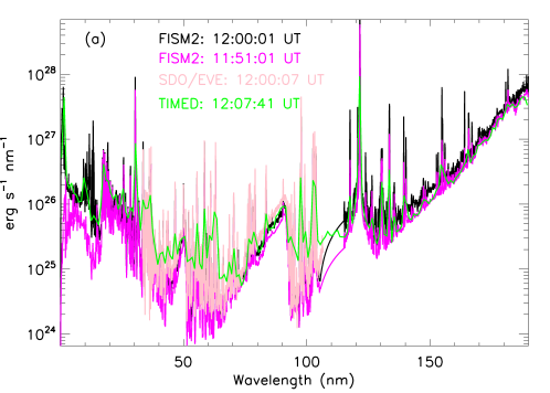
Figure 2: Solar spectra between 0.01$-$190 nm derived from FISM2 before (magenta) and during (black) the powerful flare. The overplotted spectra are measured by SDO/EVE (pink) and TIMED (green), respectively.

Figure 2 shows the solar spectrum from 0.01 nm to 190 nm derived from FISM2 with a spectral bin of 0.1 nm. The black and magenta line profiles represent the flare and quiet-Sun spectra, for instance, during the X9.3 flare and before the flare onset time. The flare spectrum from 33.35$-$106.59 nm measured by the SDO/EVE is also overplotted by the pink line, it has a time cadence of 10 s and a spectral bin of 0.02 nm (Hock et al., 2012; Woods et al., 2012). The flare spectrum (green) between 0.5$-$190 nm with a lower spectral resolution of 1 nm is observed by the Thermosphere Ionosphere Mesosphere Energetics Dynamics (TIMED) at about 12:07:41 UT, but it only lasts for about 3 minutes (Woods et al., 2005). Here, the solar spectrum observed by TIMED is used to correct the FISM2 model data, which demonstrates to match well with the observational data, as shown in Figure 2. For easier description, we simply divided the observed wavelength ranges into HXR ($<$0.1 nm), SXR (0.1$-$7 nm), EUV (7$-$120 nm), FUV (120$-$190 nm) and MUV (190$-$222 nm) (Del Zanna & Mason, 2018), while the XUV contains SXR and EUV wavelength ranges at 0.1$-$20 nm and 0.1$-$80 nm recorded by LYRA (Dominique et al., 2018).

Table 1: Instruments used in this study.

Instruments	Channels	Time cadence (s)	Wavebands	Description
	0.05$-$0.4 nm	$\sim$2.0	SXR	Flux
GOES	0.1$-$0.8 nm	$\sim$2.0	SXR	Flux
Insight-HXMT	200$-$600 keV	1.0	HXR/$\gamma$	Spectrum
Konus-Wind	331$-$1252 keV	0.256$-$8.192	$\gamma$-ray	Spectrum
	0.1$-$20 nm	0.05	XUV	Flux (gap: 2$-$6 nm)
PROBA2/LYRA	0.1$-$80 nm	0.05	XUV	Flux (gap: 5$-$17 nm)
	120$-$123 nm	0.05	Ly$\alpha$	Flux
	190$-$222 nm	0.05	MUV	Flux
	0.1$-$7 nm	0.25	SXR	Flux
	17.2$-$20.8 nm	0.25	EUV	Flux
	23.1$-$27.8 nm	0.25	EUV	Flux
SDO/EVE/ESP	28.0$-$31.8 nm	0.25	EUV	Flux
SDO/EVE/MEGS-B	33.3$-$107 nm	10	EUV	Spectrum
SDO/EVE/MEGS-P	121.6 nm	10	Ly$\alpha$	Flux
	617.3 nm	45/720	LOS/Vector	Magnetograms
SDO/HMI	617.3 nm	45	Continuum	image
SDO/AIA	9.4, 13.1, 19.3 nm	12	EUV	image
Hinode/XRT	Be_med	–	SXR	image
FISM2	0.01-190 nm	60	Empirical	Spectrum
SOHO/LASCO/C2	–	–	WL	CMEs
SOHO/LASCO/C3	–	–	WL	CMEs
SOHO/ERNE	–	–	$>$20 MeV	SEPs

3.2 Flare energy radiated in multiple wavebands

In this section, we focus on energy contents of the X9.3 flare radiated in multiple wavelengths shortward of $\sim$222 nm, for instance, the radiated energies in SXR, XUV, EUV, Ly$\alpha$, and MUV. To obtain them, we firstly remove the background emission from the solar observational irradiance. The background emission is defined as the solar irradiance before the flare onset time ($t_{o}$). Briefly, some data points before $t_{o}$ are extracted and then performed a linear fitting (Zhang et al., 2019). Then, we can calculate the radiated energy ($U_{\lambda}$) in the specific waveband ($\lambda$) by integrating the background-subtracted flux ($F_{\lambda}$) over the flare time interval (Emslie et al., 2012; Milligan et al., 2014; Zhang et al., 2019, 2021a; Cai et al., 2021), as shown in equation 1.

$$U_{\lambda}=2\pi d^{2}\int_{t_{1}}^{t_{2}}F_{\lambda}(t)\,dt,$$ (1)

Here, $d$ represents the distance between the Sun and the Earth, which is 1 AU. $t_{1}$ and $t_{2}$ are the began and stop time of the X9.3 flare in a certain waveband. It should be pointed out that $t_{1}$ and $t_{2}$ are a bit different in various channels, mainly due to the observational fact that certain-waveband radiation could be dominated in different flare phases.

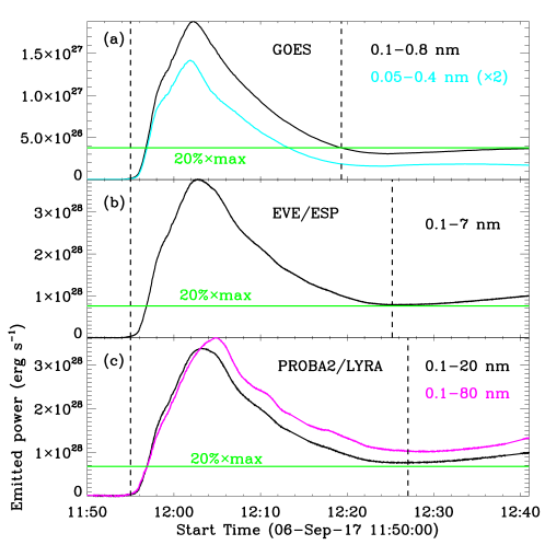
Figure 3: Background-subtracted SXR/XUV fluxes in 0.05$-$0.4 nm, 0.1$-$0.8 nm, 0.1$-$7 nm, 0.1$-$20 nm, and 0.1$-$80 nm. The vertical dashed lines marks their integrated time intervals ($t_{1}$ and $t_{2}$), and the horizontal green lines represent the 20% of their maximum (the black curve in each panel).

First of all, we calculate the flare radiated energy in SXR (0.05$-$0.4 nm, 0.1$-$0.8 nm, and 0.1$-$7 nm) and XUV (0.1$-$20 nm, 0.1$-$80 nm) wavelength ranges measured by GOES, SDO/EVE, and PROBA2/LYRA, respectively. Figure 3 presents the light curves of those five channels after removing their background emissions. It can be seen that their temporal profiles are quite similar, but their peaks appear to slightly delay in time. This is consistent with the observational fact that cooler wavelengths usually peak after the hottest ones in solar flares. That is, the flare radiation in the longer wavelength that has lower temperatures will spend much time to cool down (Kretzschmar et al., 2013). The begin time ($t_{1}$) for integrating is defined as the time when the flare starts to increase, as marked by the dashed vertical lines. It is at about 11:55:00 UT, and the GOES SXR fluxes have a 1-s deviation because the time cadence of GOES is $\sim$2 s. The stop time ($t_{2}$) for integrating is a little complicated. In Figure 1 (a), the GOES SXR flux in 0.1$-$0.8 nm reveals a second peak at roughly 12:40 UT, which is after the major flare and could affect its stop time. Therefore, $t_{2}$ is defined as the time when the flux drops to 20% of its peak value, as indicated by the green lines in panels (a) and (b). However, panel (c) shows that the XUV flux does not drop to 20% before increasing of the second peak. So, $t_{2}$ is the XUV flux decreases to its valley value, as indicated by the dashed vertical line in panel (c). Then using equation 1, the flare radiated energy in SXR and XUV wavebands is estimated, as listed in Table 2. The flare radiated energy in GOES SXR 0.1$-$0.8 nm is about 1.4$\times$10³⁰ erg, which is 3 times larger than the short-wavelength GOES channel, but it is much smaller than that radiated in ESP 0.1$-$7 nm, such as 3.4$\times$10³¹ erg. On the other hand, the flare radiated energies in two XUV channels measured by LYRA are roughly equal, which are in the order of magnitude 10³¹ erg. We want to stress that the definition of ($t_{2}$) could slightly affect the estimation of the radiated energy, i.e., about 2% (Zhang et al., 2019), but it is hardly influence for the order of magnitude.

Table 2: Radiated energy of the X9.3 flare in the specifical waveband.

Wavebands	t1 (UT)	t2 (UT)	Energy (erg)
U0.05-0.4	11:54:59	12:19:19	4.8$\times$1029
U0.1-0.8	11:54:59	12:19:19	1.4$\times$1030
U0.1-7	11:55:00	12:25:12	3.4$\times$1031
U0.1-20	11:55:00	12:27:01	3.1$\times$1031
U0.1-80	11:55:00	12:27:01	3.5$\times$1031
U17.2-20.8	11:53:57	12:27:56	4.8$\times$1029
U23.1-27.6	11:53:57	12:27:56	4.0$\times$1029
U28.0-31.8	11:53:57	12:27:56	8.2$\times$1029
U33.3-61.0	11:53:57	12:14:07	3.1$\times$1029
U61.0-79.1	11:53:57	12:14:07	1.8$\times$1029
U79.1-107	11:53:57	12:14:07	8.9$\times$1029
U190-222	11:55:16	12:07:50	1.5$\times$1030
U121.6	11:55:17	12:07:47	1.1$\times$1030

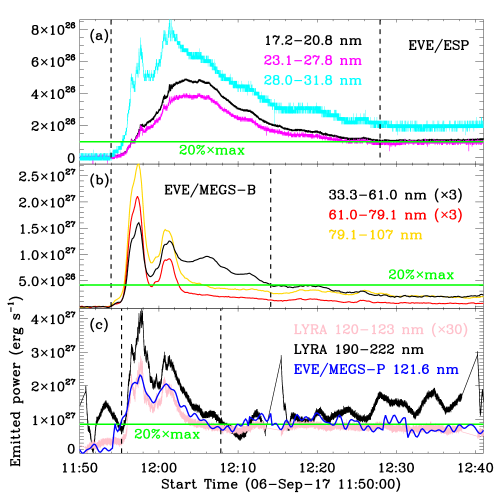
Figure 4: Background-subtracted EUV/MUV light curves in 17.2$-$20.8 nm, 23.1$-$27.8 nm, 28.0$-$31.8 nm, 33.3$-$61.0 nm, 61.0$-$79.1 nm, 79.1$-$107 nm, 120$-$123 nm, 190$-$222 nm, and 121.6 nm. The vertical dashed lines outline their integrated time intervals ($t_{1}$ and $t_{2}$), and the horizontal green lines represent the 20% of their maximum (the black curve in each panel).

Like in SXR and XUV channels, we calculate the EUV/MUV radiated energy of the X9.3 flare recorded by SDO/EVE and LYRA, as shown in Figure 4. We plot the light curves after removing their background emissions in EUV, Ly$\alpha$, and MUV wavebands, which are recorded by ESP and MEGS on board SDO/EVE, and LYRA, respectively. Here, some light curves have been multiplied by a fixed factor to show them clearly in the same window. $t_{1}$ is defined as the fixed time instance of the flare starting to increase in the chosen waveband, and $t_{2}$ is determined from the time when the radiated flux decrease to 20% of its peak value, as indicated by the dashed vertical lines. Then the radiated energy in EUV wavelengths can be estimated with equation 1. The details can be seen in Table 2. We can find that the flare radiated energy in the EUV wavelength is roughly in the order of 10²⁹ erg, which is one order less than that in the MUV and Ly$\alpha$ wavebands ($\sim$10³⁰ erg). They are much less (two order) than the radiated energy in SXR/XUV channels (10³¹ erg). This is consistent with our previous result, for instance, the radiated energy in SXR 0.1$-$7 nm recorded by ESP is similar to that in XUV 0.1$-$20 nm and 0.1$-$80 nm measured by LYRA, as listed in the fourth column of Table 2. We wanted to state that the flare energy released in the Ly$\alpha$ channel is estimated from the SDO/EVE observation, similar to the previous result (cf. Milligan et al., 2014). On the other hand, The factor $\sim$30 between SDO/EVE and LYRA is of the same order than the one found by Wauters et al. (2022) with respect to the Ly$\alpha$ channel of GOES and LYRA.

3.3 Radiative loss energy and peak thermal energy

In this section, we calculate the radiative loss energy ($U_{rad}$) and peak thermal energy ($U_{pth}$) of SXR-emitting plasmas based on the GOES and Hinode/XRT observational data. Assuming the optical thin radiation, $U_{rad}$ can be calculated with equation 2.

$$U_{rad}=\int_{t_{1}}^{t_{2}}\Lambda(T_{e}(t))\times{\rm EM}(t)\,dt,$$ (2)

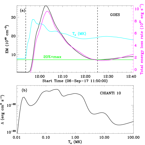
Figure 5: Panel (a): Temporal evolutions of EM (black), temperature (cyan), and total energy loss rate (magenta) obtained from the GOES SXR observation. The vertical dashed lines outline the integrated time interval, and the horizontal green lines represent the 20% of the peak EM. Panel (b): Radiative loss rate as a function of the temperature derived from CHIANTI 10.

Where $\Lambda(T_{e})$ is the radiative loss rate as a function of $(T_{e})$, which can be obtained from the CHIANTI 10 database (Del Zanna et al., 2021), as shown in Figure 5 (b). EM and $(T_{e})$ denote the emission measure and electron temperature, which are derived from two GOES SXR fluxes using an isothermal assumption (White et al., 2005), as shown in Figure 5 (a). $t_{1}$ and $t_{2}$ represent the integrated time obtained from the temporal profile of EM evolution, as indicated by the two dashed vertical lines. Then, the radiative loss energy from SXR-emitting plasmas is estimated to 8.7$\times$10³⁰ erg. Figure 5 (a) also draws the temporal evolution of the total energy loss rate (magenta) after removing the background, which is provided by the GOES team. We can calculate the total energy loss ($U_{trad}$) of hot plasmas by integrating over the background-subtracted total energy loss rate. It is estimated to about 9.0$\times$10³⁰ erg, which is roughly equal to $U_{rad}$, as can be seen in Table 3. The radiative loss energy of the X9.3 flare is 6 times larger than the radiation in GOES 0.1$-$0.8 nm, which agrees with previous observational results, for instance, one order of magnitude deviations (Emslie et al., 2012; Feng et al., 2013; Zhang et al., 2019).

Using equation 3, the peak thermal energy ($U_{pth}$) from SXR-emitting plasmas can be estimated.

$$U_{pth}\approx 3k_{b}T_{e}\sqrt{{\rm EM}\times V},$$ (3)

Here, $k_{b}$ denotes the Boltzmann constant. $V$ represents the volume of SXR-emitting plasmas, which can be estimated from the SXR image at the flare peak time observed by Hinode/XRT. The magenta contour in Figure 1 (c) outlines the major flare region contains the SXR emission at a level of $\frac{1}{e^{2}}$, which could be identified as the flare area ($A$) of SXR-emitting plasmas after correcting the projection effect (Zhang et al., 2019), such as $\sim$690 Mm². The volume can be expressed as $V=A^{\frac{3}{2}}$. Obviously, the flare area is important for estimating the peak thermal energy, since it is directly related to the volume of SXR-emitting plasmas. In this study, we also present the SDO/AIA emissions in high-temperature EUV wavelengths (13.1 nm, 19.3 nm, 9.4 nm), as indicated by the overplotted cyan, orange, and green contours in Figure 1 (c)$-$(e). Those SDO/AIA emissions include hot plasmas of the solar flare, and they match well with the SXR emission observed by Hinode/XRT, confirming the flare area of SXR-emitting plasmas. Then, $U_{pth}$ reaches its maximum when $T_{e}\sqrt{EM}$ is maximal, which is $\sim$3.1$\times$10³¹ erg. Noting that we assume a volumetric filling factor of 1.0 (e.g., Emslie et al., 2012; Zhang et al., 2019).

3.4 Nonthermal energy in flare-accelerated ions

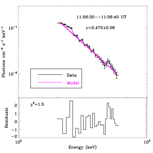
Figure 6: The Insight-HXMT spectrum with an integrated time of 10 s during $\sim$11:56:30$-$11:56:40 UT, the magenta line represents the fitting model. The spectral index ($\gamma$) and the Chi-squared residual ($\chi^{2}$) are labeled.

The HXR spectrum produced by solar flare often reveals the power-law distribution with low-energy and high-energy cutoffs, which could be a useful diagnostic of energetic electrons, protons and ions (White et al., 2011). However, the HXR spectrum below 100 keV is short of observations during the impulsive phase of the X9.3 flare (Lysenko et al., 2019). Therefore, we focus on the HXR spectrum in energy ranges between 200$-$600 keV, which is observed by Insight-HXMT, as shown in Figure 1 (b). Then, we perform a power-law model to fit the HXR spectrum (Zhang et al., 2021b). Figure 6 shows the HXR spectrum (black) and its fitting result (magenta) at the main peak of the Insight-HXMT light curve during 11:56:30$-$11:56:40 UT. The observational HXR spectrum and the fitting model appear to match well. Moreover, The Chi-squared residual ($\chi^{2}=1.5$) also implies a reasonable fitting result, i.e., $\chi^{2}<3$ (Sadykov et al., 2015). Thus, we can obtain the spectral photon index, which is about 2.472$\pm$0.063.

Next, we could estimate the nonthermal power ($P$) above a cutoff energy (E_c) for energetic electrons and protons with equation 4 (cf. Zhang et al., 2016; Li et al., 2018, 2022).

$$P(E\geq E_{c})=1.16\times 10^{24}\gamma^{3}I_{1}(\frac{E_{c}}{E_{1}})^{-(\gamma-1)},$$ (4)

Where E₁ is the lower cutoff energy. I₁ denotes the photon count rates, which has a range of 10${}^{1}-$10⁵ photon s^-1 cm^-2 at energies of E $\geq$ 20 keV and spectral indexes of $\sim$3. For the X9.3 flare, we can estimate the nonthermal energy above 200 keV by integrating the nonthermal power over a specified time interval between 11:56:30 UT and 11:56:40 UT. Using the same method, we obtain the total nonthermal energy of energetic electrons/protons from 11:56 UT to 11:59 UT during the X9.3 flare, which is about (1.5$\pm$0.2)$\times$10³¹ erg. At last, we estimate the nonthermal energy (E_nth) of all accelerated ions above 200 keV by assuming that the total ion energy could be three times larger than the electron/proton energy (Emslie et al., 2012; Aschwanden et al., 2017), for instance, E${}_{nth}\sim$4.5$\times$10³¹ erg, as listed in Table 3. As Insight-HXMT does not measure the entire duration of the HXR/$\gamma$-ray emission, our measurement of the nonthermal energy is indeed a minimum estimation.

Table 3: Energy components for the X9.3 flare.

Urad	Utrad	Upth	Enth
8.7$\times$1030 erg	9.0$\times$1030 erg	3.1$\times$1031 erg	$\geq$4.5$\times$1031 erg

4 Energetics of the accompanied CME

Here, we first calculate basic quantities such as mass, height, and speed, and then derive the gravitational potential and kinetic energies of the accompanied CME. Traditionally, the mass is estimated according to the Thomson scattering theory by assuming that all of the emission along a given LOS comes from electrons located on the Thomson Sphere (where the scattering angle equals to 90^∘ and the Thomson scattering is the most efficient). For the FOV ($<$ 30$R_{\odot}$) of the LASCO/C2 and C3, the Thomson Sphere virtually coincides with the plane of sky (POS), which means that the traditional method is only reliable for CMEs that propagate along or close to the POS. In the case of CMEs propagating away from the POS, especially Halo CMEs, the Thomson scattering drastically drops and more electrons are expected to reproduce the observed white-light intensity, which increases the uncertainties in the mass determinations. However, such uncertainties can be partly reduced by assuming that all the electrons contributing to the white-light emission lies on a different angle than the POS (Vourlidas et al., 2010). This angle should be the propagation angle of the CME with respect to the POS.

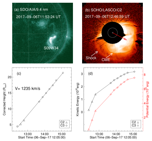
Figure 7: Physical properties of the CME on 6 September 2017. Panel (a): Solar disk image taken by SDO/AIA at 9.4 nm. (b) Coronal image taken by SOHO/LASCO/C2. The small white circle inside the occulter represents the solar disk, with the“+” symbol indicating the solar center. The dotted line outlines the CME projected on the plane of sky. The “$\ast$” symbol indicates the projected location of the CME mass center. (c) Height-time profile of the CME mass center. A linear fit of the profile reveals an average speed. (d) Evolution of kinetic (black) and potential (red) energies of the CME. The “$\triangle$” and “$\diamond$” symbols show measurements from LASCO/C2 and C3, respectively.

In our case, as seen in Figure 7 (a) and (b), the CME under study originates from active region NOAA 12673 located at about 56 degree from the west solar limb. Assuming that the CME propagates radially from the source active region (Reiner et al., 2003; Kahler & Vourlidas, 2005), the CME angle of propagation with respect to the POS is estimated to be about 56 degree. Base on this angle and the Thomson scattering formulation (Billings, 1966), the coronal images containing the CME, after subtracting a suitable pre-event image, can be converted to the corresponding mass images. The total mass of the CME ($M_{cme}$) is computed by summing the masses in the pixels encompassed in the CME, as delineated by the black dotted line in Figure 7 (b). The radial height ($R_{mc}$) of the mass center of the CME from the solar center is given by equation 5.

$$R_{mc}=\frac{\sum m_{i}r_{i}}{\sum m_{i}},$$ (5)

Here $m_{i}$ is the mass in each pixel, r_i is the corrected POS height of each pixel (POS height divided by cosine of the CME propagation angle). We calculate $R_{mc}$ for each of the coronal images as the CME propagated through the field of view of LASCO. Figure 7 (c) shows the evolution of the height of the CME mass center. A linear fit to the height-time data reveals an averaged velocity ($v_{cme}$) of $\sim$1235 $\rm{km~{}s}^{-1}$ for the CME. The calculation of the height and speed as described above has an advantage of involving only the measurement of the CME mass center. Based on the computed mass, height, and velocity, the potential ($E_{p}$) and kinetic ($E_{k}$) energies of the CME can be simply estimated by equation 7.

$$E_{p} = GM_{\odot}M_{cme}(\frac{1}{R_{\odot}}-\frac{1}{R_{mc}}),$$ (6)

$$E_{k} = \frac{1}{2}M_{cme}v_{cme}^{2},$$ (7)

Where $G$ is the gravitational constant, $M_{\odot}$ and $R_{\odot}$ represent the mass and radius of the Sun. Here, we measure the potential energy relative to the solar surface, and the obtained results are illustrated in Figure 7 (d). As can be seen, both the kinetic energy and the potential energy of the CME increase with time (and hence the altitude). The kinetic energy is obvious larger than the gravitational potential energy, and the total CME energy is about 4$\times$10³² erg. Note that, the CME is partially occulted by the coronagraph mask at early times, which leads to an underestimation of the CME energy.

5 Magnetic free energy

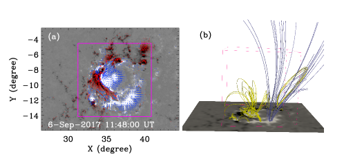
Figure 8: Panel (a): SDO/HMI vector magnetogram of the AR NOAA 12673 hosting the flare and CME. Panel (b): Nonpotential magnetic configurations derived from the NLFFF extrapolation. The yellow and purple lines represent the closed and open magnetic field lines, respectively. The magenta box outlines the region that is used to calculate the magnetic free energy.

In order to estimate the magnetic free energy stored in the AR NOAA 12673, we perform a nonlinear force-free field (NLFFF) extrapolation using the ‘weighted optimization’ method (Wheatland et al., 2000; Wiegelmann et al., 2012) after preprocessing the photospheric boundary to meet the force-free condition (Wiegelmann et al., 2006), as shown in Figure 8. This method uses the photospheric magnetic field vector (panel a) observed by the SDO/HMI and the potential field derived from the vertical component of the magnetic field with a Green’s function algorithm as a boundary condition to reconstruct three-dimensional magnetic fields. For the extrapolation, we bin the data to 1.0^′′ pixel^-1 and adopt a computation box of 300$\times$224$\times$224 uniform grid points (225$\times$168$\times$168 Mm³). Panel (b) presents the NLFFF extrapolated results, and it shows both the closed and open magnetic field lines, but the open magnetic field lines prefer to appear at the non-flare area. The magnetic free energy (E_free) can be determined from the NLFFF (E_nl) energy and the potential field energy (E_pf) with equation 8

$$E_{free}=E_{nl}-E_{pf}=\int_{V}\frac{B_{nl}^{2}-B_{pf}^{2}}{8\pi}\,dV,$$ (8)

Here, B_nl and B_pf represent the magnetic strength of the nonpotential and potential fields, which can be obtained from the NLFFF extrapolation. $V$ stands for the coronal volume of the AR, and a value of about 120$\times$120$\times$120 Mm³ is taken into consideration here, as indicated by the magenta box in Figure 8. Thus, the magnetic free energy can be estimated to about 2$\times$10³³ erg.

6 Energy of SEPs

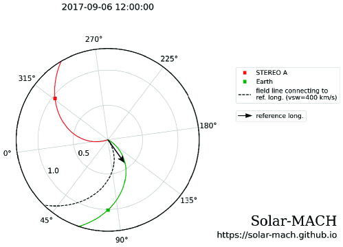
Figure 9: Positions of the Earth (green) and STEREO-A (red) as seen from the northern ecliptic pole on 6 September 2017. Also shown are the Parker spirals connecting to Earth and STEREO-A, as well as the reference longitude of the eruption given by the position of the solar flare.

The solar eruption of 6 September 2017 was magnetically well connected to Earth, as shown in Figure 9, which depicts the Parker spirals connecting to Earth (green) and STEREO-A (red) for a nominal solar wind speed of 400 km s^-1. The black arrow indicates the direction of the eruption based on the location of the associated flare, assuming radial propagation. Indeed, a solar energetic particle (SEP) event was detected near Earth, but not at STEREO-A, which was separated from the eruption by almost 180^∘.

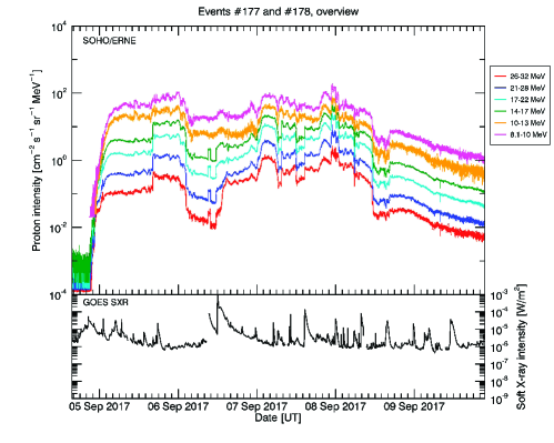
Figure 10: Proton intensities as measured by the ERNE instrument aboard SOHO in the period of 5 to 10 September 2017. For comparison, the GOES SXR flux is shown in the lower panel. The increase of the proton flux associated with the X9.3 flare peaking at 12:02 UT on 6 September is most clearly seen at the highest energies.

Inspection of all available particle data near Earth has revealed that at lower energies, the event is strongly contaminated by particles associated with several previous events on September 5 and 6. The only clear signature of the event suitable for further analysis was found in high-energy proton data as detected by the ERNE instrument (Torsti et al., 1995) aboard SOHO. Figure 10 shows the ERNE proton intensities and the GOES soft X-ray flux in the period of 5 to 10 September 2017. It is evident that our event is best seen at the highest energies.

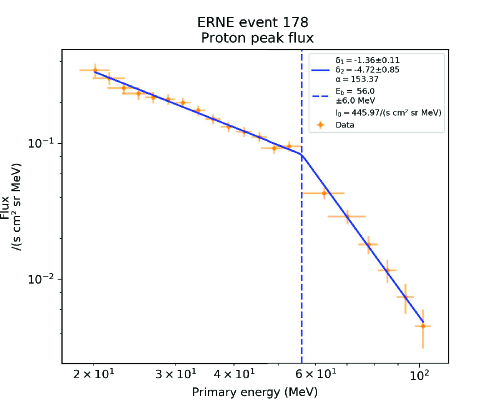
Figure 11: Proton peak flux spectrum as derived from the ERNE data for particle event of 6 September 2017 in the range of 20 MeV to 100 MeV. The data is shown as orange crosses, a spectral fit is indicated as a blue line, and the fit parameters are indicated in the legend.

In the following, we first consider the energetics of the prompt SEP component, before deriving the energy of the total SEP population. For the prompt component, we have used the ERNE data above 20 MeV to obtain the proton peak flux spectrum which is shown in Figure 11. The flux profiles were fitted with a function, i.e., a modified Weibull profile given by Kahler & Ling (2017). We have fitted the peak flux spectrum $I_{\rm p}(E)$ with a broken power-law (cf. Strauss et al., 2020), which includes a smooth transition at the spectral break according to:

$$I_{\rm p}(E)=I_{0}\left(\frac{E}{E_{0}}\right)^{\delta_{1}}\left(\frac{E^{\alpha}+E^{\alpha}_{\mathrm{b}}}{E^{\alpha}_{0}+E^{\alpha}_{\mathrm{b}}}\right)^{\frac{\delta_{2}-\delta_{1}}{\alpha}},$$ (9)

where E is particle energy, $I_{0}$ the flux at a reference energy $E_{0}=0.1$ MeV, $\delta_{1}$ and $\delta_{2}$ the spectral indices below and above the break energy $E_{\mathrm{b}}$, and $\alpha$ the parameter describing the smoothness of the transition. The best-fit parameters are indicated in Figure 11.

This SEP event was characterized by strong scattering, with particles repeatedly passing back and forth through the position of the spacecraft. We therefore adopt an approach (cf. Wibberenz et al., 1989) in order to relate the measured peak flux spectrum $I_{\rm p}(E)$ at 1 AU to the proton fluence spectrum injected at the source surface, which is based on diffusive transport of protons in the interplanetary medium. Therefore, we can use the peak flux spectrum as a measurement of the accelerated proton spectrum at the Sun,

$$\frac{{\rm d}N}{{\rm d}E}=\frac{4\pi r^{3}_{0}}{0.925v}I_{\rm p}(E),$$ (10)

where $N$ is the number of accelerated protons, $v$ is the particle speed (recall that ${\rm d}E=v\,{\rm d}p$), and $r_{0}$ is the distance from the Sun. ${\rm d}N/{\rm d}E$ represents the total number of accelerated particles per steradian at the source surface and per unit energy.

For the prompt SEP component, we have to consider two different scenarios for constraining the area on the source surface over which energetic particles are injected: either acceleration at a CME-driven shock wave, or acceleration (and subsequent escape along open magnetic field lines) in the solar flare. Considering the first possibility and assessing the extent of the CME (cf. Figure 7), adopting a solid angle of 2$\pi$ (i.e., a full hemisphere) appears to be reasonable. Integrating from 20 MeV up to 100 MeV and multiplying with particle energy, we finally obtain an energy in accelerated protons above 20 MeV of $1.4\times 10^{28}$ erg. Assuming that the power-law extends to lower energies with the same index $\delta_{1}$, we can derive estimates for the total proton energy content. Extrapolating down to 50 keV, we get an energy of $5.1\times 10^{28}$ erg.

Next, we consider the alternative scenario where the protons are accelerated in the solar flare and subsequently propagate to interplanetary space along open magnetic field lines. We used a PFSS (potential field source surface) extrapolation based on a synoptic SDO/HMI map to determine the area on the source surface that connects back to the flaring area. For the source surface, we used three different heights: 2.5, 2.0 and 1.5 solar radii (heliocentric distance). The standard height is usually taken as 2.5 solar radii, but Virtanen et al. (2020) have shown that the source surface has, for the last two decades, seemed to stay below 2.0 solar radii. Surprisingly, we found that there are no open magnetic field lines connecting to the flare site, even if we lower the source surface all the way down to 1.5 solar radii. While active regions are predominantly closed-field regions, normally a PFSS extrapolation does show some open field lines. We cannot rule out the possibility of some open field lines were formed by magnetic reconnection in the flare site, since the synoptic HMI maps and the PFSS model cannot take into account those relatively short-lived processes. However, even if this actually had been the case, the corresponding area on the source surface would have been small. Taking the flare area as an estimate, we derive a total SEP energy of only $5.1\times 10^{28}$ erg.

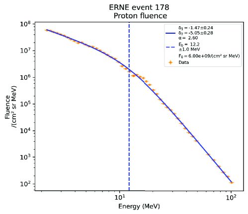
Figure 12: Proton fluence spectrum as derived from the ERNE data for particle event of 6 September 2017 in the range of 2 MeV to 100 MeV. The data is shown as orange crosses, a broken power-law fit is indicated as a blue line, and the fit parameters are indicated.

We now consider the energetics of the total SEP population. The work by Mewaldt et al. (2008) is widely recognized as the pioneering in SEP energetics, and a comprehensive study has been given by Emslie et al. (2012). For a sample of 38 solar eruptive events, they obtained SEP energetics ranging from $1.3\times 10^{29}$ erg to $4.3\times 10^{31}$ erg. In order to compare with these results, we apply their methodology to our event. The observed fluence (in units of cm^-2) at 1 AU is converted to on-axis fluence assuming a Gaussian in latitude and longitude with a width of $\sigma=38^{\circ}$ centered at the flare location (9S,34W) and a solar wind speed of 450 km s^-1, i.e., a connection point at (7N,52W). This implies an increase of the fluence by a factor of 1.22. Then the Gaussian fluence distribution is integrated over longitude and latitude and multiplied by (1 AU)²; this implies a further factor of $6.21\times 10^{26}$ cm². Finally, we apply a factor 0.5 to account for the multiple-crossing effect. Thus, the total factor to apply here is $3.8\times 10^{26}$ cm². We obtain the total proton fluence from the ERNE spectrum shown in Figure 12 by integrating the spectrum 50 keV to 400 MeV and applying the correction factor. This gives a total energy of about $10^{31}$ erg, which is already comparable to the largest values derived by the previous finding (cf. Emslie et al., 2012). Thus, the prompt component of this SEP event contains a negligible fraction of the SEP energy, and almost all of it is due to the interplanetary acceleration.

7 Discussions

The X9.3 flare on 6 September 2017 is the most powerful flare during the solar cycle 24, and it has been studied by several authors (e.g., Dominique et al., 2018; Kolotkov et al., 2018; Lysenko et al., 2019; Karlický & Rybák, 2020; Motorina et al., 2020; Lee et al., 2021; Li et al., 2021b; Zhang et al., 2021b). In this work, we explored the energy partition in the X9.3 flare. Based on multi-instrument measurements, we calculated the flare radiated energy in X-ray and UV wavelength ranges, as listed in Table 2. It can be seen that the maximal energy during the X9.3 flare is measured by LYRA at 0.1$-$80 nm, which is about 3.5$\times$10³¹ erg. It is roughly equal to that measured by EVE/ESP 0.1$-$7 nm, such as 3.4$\times$10³¹ erg. They are $\sim$20 times bigger than the radiated energy in GOES 0.1$-$0.8 nm, which is similar to previous observations (Zhang et al., 2019; Cai et al., 2021). The flare radiated energy observed by LYRA in 0.1$-$20 nm is about 3.1$\times$10³¹ erg, and it is a bit smaller than that in ESP 0.1$-$7 nm. This is mainly because that there is a drop of the spectral response in the middle of the bandpass in this channel, for instance, a gap in the responsivity between 2$-$6 nm (cf. Dolla et al., 2012; Dominique et al., 2013). On the other hand, the flare energy radiated in EUV wavelengths is in the order of 10²⁹ erg, which is much smaller than that radiated in the SXR channel, i.e., two orders of magnitude. While the flare radiated energy in Ly$\alpha$ and MUV increases slightly, could be about 10³⁰ erg, but still less than that in the SXR channel of 0.1$-$7 nm. Our observations suggest that the flare emission mainly comes from the shorter wavelength, for instance, the major contribution of the flare radiation comes from the SXR emission at 0.1$-$7 nm, while there is actually quite few contribution coming from the EUV ranges. It should be pointed out that here the flare radiation between 0.1$-$222 nm is studied due to observational limitations, and thus the observational result is only applicable to this wavelength range. In fact, most of the flare energy is radiated in the wavelength longward of 200 nm, for instance, the radiated energy in the WL continuum could be as high as 70% (cf. Kretzschmar, 2011; Kleint et al., 2016). However, the major contribution from the WL continuum is impossible estimated due to the lack of observations, since the HMI continuum represents the true WL continuum only in the quiet sun, while it can be significant deviations in the flare (Švanda et al., 2018). On the other hand, a majority of the flare energy is released in the wavelength shortward of 27 nm, i.e., about 19% , while very little flare energy is radiated in EUV passbands (e.g., Woods et al., 2004; Kretzschmar et al., 2010). Therefore, we could assume that the total solar irradiance (TSI) of the X9.3 flare is about 3$\times$10³² erg. We wanted to state that the flare energy in the radio emission is not estimated, mainly due to its rather low contribution to the total TSI (Pasachoff, 1978).

According to the standard flare model (Masuda et al., 1994; Priest & Forbes, 2002; Shibata & Magara, 2011), the flare radiated energy in multiple wavelengths could convert from either thermal or nonthermal energies. In this study, we also calculate the peak thermal energy of SXR-emitting plasmas and the nonthermal energy, which are estimated to about 3.1$\times$10³¹ erg and 4.5$\times$10³¹ erg. Similar to previous observations (Emslie et al., 2012; Feng et al., 2013; Zhang et al., 2019; Cai et al., 2021), they are adequate sufficient to support the radiative loss energy (U_rad) of hot plasmas, as seen in Table 3. However, the thermal and nonthermal energies are smaller than the TSI of the X9.3 flare in full wavebands. The peak thermal energy from GOES is based on the assumption of an isothermal temperature (White et al., 2005; Emslie et al., 2012), but the solar flare often shows multi-thermal temperatures, for instance, the multi-thermal flare loops (Aschwanden et al., 2015; Li et al., 2021a). Hence, our measurement of the peak thermal energy could be regarded as the lower limit estimation using two GOES SXR fluxes. The radiative loss energy in our case is a little smaller than the previous result (Motorina et al., 2020), who used a much long-time integration between 11:53$-$13:40 UT. We use the short-time integration because that the GOES flux (Figure 1 a) shows a growth trend after $\sim$12:30 UT, which might be regarded as another flare. Moreover, the EUV, Ly$\alpha$, and MUV fluxes do not exhibit the similar growing trend. We should state that the energy spectrum of the X9.3 flare captured by Insight-HXMT is from about 100 keV to 800 keV (Zhang et al., 2021b), and here we only fit the energy range between 200$-$600 keV every 10 s to improve the signal to noise ratio. Our estimation of the nonthermal energy is larger than the total ion energy (1.1$\times$10³¹ erg) estimated from the Konus-Wind observation (Lysenko et al., 2019; Motorina et al., 2020). This is because that the available observational data of Konus-Wind only remains about 72 s, which is much shorter than Insight-HXMT observations (Figure 1 b). Similar to Konus-Wind (Lysenko et al., 2019), Insight-HXMT misses the credible data below the energy of 200 keV for the X9.3 flare. Thus, the energy spectrum fitting tend to the higher energetic electrons/pronotos, but lack of the lower energetic electrons. Hence, our measurement of the nonthermal energy is also the minimum estimation using the Insight-HXMT spectrum. Therefore, the actual thermal and nonthermal energies could be large enough to support the TSI of the X9.3 flare.

Based on WL continuum images measured by LASCO/C2 and C3, we estimate the mass and height of the CME followed by the X9.3 flare, as well as the propagation speed of the CME. Then, we obtain its kinetic and gravitational potential energies, as shown in Figure 7. It can be seen that the kinetic energy of the CME is a bit larger than the gravitational potential energy, which is mainly related to the fast propagation speed of the CME (Aschwanden et al., 2016). Our observational results agrees with previous findings for the energy distribution of CMEs (Emslie et al., 2004, 2012). Conversely, some authors (Vourlidas et al., 2000; Ying et al., 2018) also found that the majority CME energy is from the gravitational potential energy, but for those CMEs have slower propagation speeds, i.e., $<$500 km s^-1. The total CME energy here is estimated to $\sim$4$\times$10³² erg, which is roughly equal to the flare energy (Emslie et al., 2005; Feng et al., 2013; Ying et al., 2018). We want to stress that the magnetic energy taken by the CME is not estimated, since the magnetic field strength in the CME is unknown.

It is well accepted that both the flare and CME energies are released from the magnetic fields in solar disk, such as the AR. Hence, we calculate the magnetic free energy released from the AR NOAA 12673 on the Sun. Using the SDO/HMI vector magnetogram before the X9.3 flare, the nonpotential and potential fields are estimated by the NLFFF extrapolation (Wheatland et al., 2000; Wiegelmann et al., 2006, 2012). Then, the magnetic free energy can be estimated to roughly 2$\times$10³³ erg, which is one order of magnitude larger than the flare and CME energies. Our estimations suggest that the magnetic free energy released by the solar AR is adequate enough to power the major flare and its accompanied CME, which agrees with previous findings for the eruptive (Feng et al., 2013; Aschwanden et al., 2016).

At last, we have estimated the energy content of the SEPs. The contribution from prompt SEPs was negligible, which is consistent with the strong magnetic containment in the associated flare. Comparing the total SEP energy with the CME energy, we find that the SEPs contain about 2.5% of the CME energy. This is consistent with previous values obtained by Emslie et al. (2012) who found fractions of 1–10%, and shows that the CME was quite efficient in accelerating SEPs in interplanetary space.

8 Summary

Using coordinated observations measured by multiple instruments, for instance, GOES, Insight-HXMT, PROBA2/LYRA, SDO/EVE, SDO/HMI, SDO/AIA, Hinode/XRT, SOHO/LASCO, and SOHO/ERNE, we evaluate the energetics of a powerful flare, the accompanied CME and SEPs on 6 September 2017. Our major results are summarized in following:

1. We focus on the flare radiated energy in SXR, EUV, Ly$\alpha$, and MUV wavelength ranges, although the major contribution of the TSI is from the WL continuum. However, we did not find the WL continuum data for the X9.3 flare. In the studied wavelength ranges, the flare radiated energy in the SXR 0.1$-$7 nm is much larger than other wavebands, which is $\sim$3.4$\times$10³¹ erg. Only a small amount of flare energy emitted at the EUV wavelength, such as in the order of 10²⁹ erg. At wavebands of Ly$\alpha$ and MUV, the flare radiated energy could be in the order of 10³⁰ erg.

2. The total radiated energy of the X9.3 flare could be as high as $\sim$3$\times$10³² erg, which is almost in the energy realm of the stellar flare. The peak thermal energy is estimated to be $\sim$3.1$\times$10³¹ erg, assuming an isothermal temperature for the flare. The nonthermal energy is also estimated to $\sim$4.5$\times$10³¹ erg. Both the thermal and nonthermal energies are minimum estimations, mainly due to the limitation of observational data.

3. The energy content of the accompanied CME is estimated, which has a total energy of $\sim$4$\times$$10^{32}$ erg. The kinetic energy of the CME is larger than the potential energy, and they both increase with the altitude.

4. The released energy from the X9.3 flare is comparable to the energy carried by the CME. The magnetic free energy stored in the AR is estimated to about 2$\times$$10^{33}$ erg with the NLFFF extrapolation, and it is able to support the powerful flare and CME eruptions.

5. The SEP energy content is estimated as about 10³¹ erg for protons in the range of 50 keV to 400 MeV, which amounts to 2.5% of the CME energy. A negligible fraction was contributed by the prompt SEP component. Thus, the CME was very efficient in accelerating particles in interplanetary space.

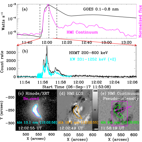
Figure 1: Overview of the powerful flare on 6 September 2017. Panels (a) and (b): Multi-wavelength light curves measured by GOES, SDO/HMI, HXMT, and Konus-Wind. Panel (c): Snapshot observed by Hinode/XRT, the overplotted magenta contour represents the SXR emission at a level of 1/e². Panel (d): LOS magnetogram measured by SDO/HMI. Panel (e): Pseudo-intensity image obtained by SDO/HMI continuum data, two magenta arrows point out the locations where the while light enhancements took place. The overplotted cyan, orange, and green contours are made from SDO/AIA emissions. The magenta rectangle marks the integrated region for the light curve in white continuum.